Approaching probabilistic and deterministic nomic truths in an inductive probabilistic way

Abstract

Theories of truth approximation in terms of truthlikeness (or verisimilitude) almost always deal with (non-probabilistically) approaching deterministic truths, either actual or nomic. This paper deals first with approaching a probabilistic nomic truth, viz. a true probability distribution. It assumes a multinomial probabilistic context, hence with a lawlike true, but usually unknown, probability distribution. We will first show that this true multinomial distribution can be approached by Carnapian inductive probabilities. Next we will deal with the corresponding deterministic nomic truth, that is, the set of conceptually possible outcomes with a positive true probability. We will introduce Hintikkian inductive probabilities, based on a prior distribution over the relevant deterministic nomic theories and on conditional Carnapian inductive probabilities, and first show that they enable again probabilistic approximation of the true distribution. Finally, we will show, in terms of a kind of success theorem, based on Niiniluoto’s estimated distance from the truth, in what sense Hintikkian inductive probabilities enable the probabilistic approximation of the relevant deterministic nomic truth. In sum, the (realist) truth approximation perspective on Carnapian and Hintikkian inductive probabilities leads to the unification of the inductive probability field and the field of truth approximation.

1 Introduction

Theories of truth approximation in terms of truthlikeness (or verisimilitude) almost always deal with (non-probabilistically) approaching deterministic truths, either actual or nomic, and have a Popperian background. E.g. Graham Oddie’s Likeness to truth (1986) and Ilkka Niiniluoto’s Truthlikeness (1987) focus on deterministic actual truths. My own From Instrumentalism to Constructive Realism (Kuipers, 2000) and Nomic truth approximation revisited (Kuipers, 2019) deal almost exclusively with (qualitatively) approaching deterministic nomic truths, based on the hypothetico-deductive method.

This paper deals first with approaching a probabilistic nomic truth, viz. a true probability distribution. It assumes a multinomial probabilistic context, hence with a lawlike true, but usually unknown, distribution. Approaching this true multinomial distribution can naturally be based on Carnapian inductive logic or inductive probability theory (Kuipers, 1978). Assume e.g. random sampling with replacement in an urn with colored balls. The primary problem of truthlikeness, or verisimilitude, is the logical problem of finding an optimal definition. In the present context this amounts to an optimal definition of the distance between any (multinomial) probability distribution and the, presumably unknown, true distribution. There are some plausible standard measures. However, the epistemic problem of verisimilitude is at least as interesting: what is a plausible distribution to start with, and how to update it in the light of empirical evidence such that convergence to the true distribution, that is, truth approximation, takes place. It will be shown that Carnap-systems, starting from equal probabilities, converge in an inductive probabilistic way to the corresponding true probabilities, i.e. the true multinomial distribution (or the probabilistic nomic truth).

Next we will introduce Hintikkian inductive probabilities, based on a prior distribution over the relevant deterministic nomic theories (a kind of constituents) and on conditional Carnapian inductive probabilities, and show that they enable again probabilistic approximation of the true multinomial distribution. Hintikkian systems add to this the inductive probabilistic convergence to the true constituent, i.e., the deterministic nomic truth about which conceptual possibilities are nomically possible, here specified as those which have a positive true probability. However, on second thoughts it is problematic to call this a genuine form of truth approximation. It turns out to be more plausible to take into account Niiniluoto’s notion of estimated distance to the truth, which can be based on the Hintikkian probabilities. Hence, if applied in the random sampling context, both Carnapian and Hintikkian types of systems can be reconstructed as inductively approaching a probabilistic nomic truth and, in the Hintikka-case, in addition as inductively approaching a deterministic nomic truth in terms of a decreasing estimated distance from the truth.

Some more background may be useful. The focus in this paper is, like in Kuipers (2000, 2019), on nomic truths, that is, truths dealing with which conceptual possibilities are nomically, e.g. physically or biologically, possible and which ones are not, the nomic (im-)possibilities, for short. A deterministic nomic truth just states which conceptual possibilities are nomically possible. A probabilistic nomic truth is in fact more detailed. It states the objective probabilities (if applicable) of the conceptual possibilities, non-zero for the nomic possibilities and zero for the nomic impossibilities. Objective probabilities are conceived of as objective dispositions or tendencies of a device to generate outcomes of which the relative frequencies have limits corresponding to these objective probability values. (Note that we do not deal with the logical possibility of nomic possibilities with zero probability.) In sum, nomic truths describe lawlike behavior of some kind or another. Since we will exclusively deal with nomic truths, deterministic or probabilistic, we will not always insert ‘nomic’ where it would be appropriate.

Now there are at least three options for nomic truth approximation:

• Option 1. Non-probabilistically approaching a deterministic nomic truth.

• Option 2. Probabilistically approaching a probabilistic nomic truth.

• Option 3. Probabilistically approaching a deterministic nomic truth.

As suggested before, Option 1 has been the primary focus of research explicitly dealing with truth approximation. As reflected in the title, this paper deals primarily with Options 2 and 3, using inductive probabilities, but we will need some aspects of Option 1, in the rest of this introduction and in Sects. 4 and 6. For the logically possible fourth option, i.e. non-probabilistically approaching a probabilistic nomic truth, we see no meaningful interpretation.

As far as Kuipers (2000, 2019) are concerned, Option 1 deals primarily with qualitative (basic, refined, and stratified) ways of approximation of a deterministic nomic truth. A consequence of the basic definition of closer to the truth in this approach will play a recurrent role in this paper. The definition itself is given in terms of sets of conceptual possibilities (X, Y), and amounts to a (set-theoretically) decreasing symmetric difference with the set T of nomic possibilities:

$$ Y\;{\text{is}}\Delta-\text{closer}{\text{to}}\;T\left( { = {\text{set}}\;{\text{of}}\;{\text{nomic}}\;{\text{possibilities}}} \right){\text{than}}\;X\;{\text{iff}}\;Y\Delta T \subset X\Delta T $$

It is important to note that in the context of nomic deterministic truth approximation, theories X and Y amount to the (maximal) claims X = T and Y = T, respectively. Of course, these claims are mutually incompatible. Following the terminology of Niiniluoto (1987), the definition is restricted to complete answers to the cognitive problem which subset of conceptual possibilities corresponds to the true one, i.e. T. Hence, in the case that for example Y is a subset of X, the claim of Y does not entail that of X, as one might think, the two claims are incompatible.¹²

Together with a corresponding definition of ‘more successful’ it is possible to prove the crucial (basic) success theorem. It states that a theory which is Δ-closer to the nomic truth than another is always at least as successful and in fact, under some plausible conditions, more successful in the long run. The idea of something like a success theorem in other cases will play a guiding role in the paper.

In Sect. 2 we will introduce, for a ‘multinomial context’, the true multinomial distribution (the probabilistic nomic truth) and candidate probability distributions (probabilistic nomic theories) for approaching it (Option 2), and prove a restricted success theorem. Section 3 studies the extent to which the true multinomial distribution can be approached by Carnapian inductive probabilities. Section 4 deals with the basics of deterministic nomic truth and deterministic nomic theories approaching it (Option 1). In Sect. 5 we introduce Hintikkian inductive probabilities, based on a prior distribution over the relevant deterministic theories and conditional Carnapian inductive probabilities, enabling again probabilistic approximation of the true multinomial distribution (Option 2). In Sect. 6 we show, based on a kind of success theorem, in what sense Hintikkian inductive probabilities enable the probabilistic approximation of a deterministic nomic truth (Option 3), viz. in terms of Niiniluoto’s estimated distance from the truth. Section 7 presents some concluding remarks.

Carnap- and Hintikka-systems of inductive probabilities were the crucial focus of my dissertation (Kuipers, 1978). After more than 40 years, I begin to understand that it can best be seen in light of approaching probabilistic nomic truths, that is, of approaching the relevant true probability distribution. This, evidently, realist perspective³ leads to the unification of the two research fields, that is, the inductive probability field and the field of truth approximation. As a matter of fact, I consider all approaches to a true probability distribution, and therefore all (perhaps frequency interpreted) inferential statistics also to be approaches to the truth.

To be sure, much of what is presented in this paper is not new. The goal of the paper is a systematic presentation of what systems of inductive probability of Carnapian and Hintikkian style can offer from the perspective of probabilistic truth approximation, in particular the epistemological problem. This leads to the search for relevant success theorems: does ‘closer to the truth’ entail ‘more successfulness’? In addition, besides presenting some well-known evidence-based logical (or internal or ‘with certainty’) conditional, stepwise and limit results, we will study, assuming an underlying multinomial experiment, the objective (or external and, a number of times, ‘with probability 1’) conditional, stepwise and limit behavior of such systems. In both cases, some well-known theorems of arithmetic and probability theory will be used.

Both types of results show that it is perfectly possible to combine the inductive probabilistic and the truth approximation perspective, both in the logical and the objective sense. This is contrary to what was (and still is?) believed in empiricist, Carnapian circles and realist, Popperian circles. In fact this paper extends the claim in Kuipers (2000) that in the context of deterministic theories the inductive instrumentalist methodology is perfectly compatible with the realist truth approximation perspective. In both cases holds that even ‘inductivists’ who are reluctant to subscribe to the truth approximation perspective are in practice approaching the truth in certain contexts, that is, whether they like it or not.

We conclude this section with some clarifications regarding the specific relation of this paper to other work.

There are many ways how to estimate the bias of a multinomial experiment, for example random sampling with replacement, a wheel of fortune or roulette, statistically, e.g. by (Bayesian) Dirichlet distributions or frequentist means. It is plausible that these statistical methods can be rephrased and further articulated in terms of inductive probabilities and (increasing) verisimilitude. For example, Festa (1993) showed the equivalence of certain Dirichlet distributions and (generalized) Carnap-systems and studied optimization of the latter from the truth approximation perspective.

As stated before, here we restrict our attention to the study of the inductive methods of Carnap and Hintikka from the perspective of truth approximation. Whereas standard statistical methods seem to go straight to their target, whether or not called ‘the truth’, the two inductive methods were designed to learn, with a self-chosen speed, from experience in a systematic and conceptually transparent way, without (Carnap) or with (Hintikka) some objective target, the truth, in mind. Whereas Carnap focused on one-step prediction probabilities, Hintikka focused on, using Carnap-systems, probabilities for generalizations. The surplus value of such inductive systems in particular when seen in the truth approximation perspective is that they articulate leading intuitions of layman and scientists, in particular other than statisticians, and hence they enable conceptually transparent communication.

As said, Roberto Festa (1993, Part III) studied already (generalized) Carnap-systems from the perspective of truth approximation, but his focus was not on the (logical or objective) limit behavior, but on the logical and epistemic ‘problem op optimality’. That is, the logically and epistemically optimal choices of parameters, the former in view of the objective probabilities [in fact a generalization of Carnap (1952, Section 2)] and the latter in view of the background knowledge.

As is well known, Hintikka (1966) introduced stratified systems of inductive probability, based on Carnap-systems, leaving room for generalizations, and he assumed a particular prior distribution over generalizations. He focused on, among other things, the logical limit behavior of such systems, leading to ‘with certainty results’: like Carnap-systems, the ‘special values’ converge to the relative frequency, and the probability of the strongest generalization compatible with the evidence converges to 1, assuming that this strongest generalization remains constant.

In his monumental book on truthlikeness, Niiniluoto (1987) focused, regarding the epistemic problem of verisimilitude, primarily on the momentary ‘evidence-based’ probabilistic estimation of the distance of a deterministic theory from the deterministic truth, based on a quantitative distance measure between theories. However, in Sect. 9.5 on the estimation problem for (deterministic, monadic) generalizations, where the relevant truth is a deterministic generalization, he includes also the logical (with certainty) limit behavior of the estimated distance from the truth, along the lines of Hintikka.

As suggested before, besides incorporating ‘with certainty’ results, we concentrate on the objective conditional, stepwise and limit behavior of such systems, frequently, not ‘with certainty’, but ‘with probability 1’.

As before indicated, we will use the phrases ‘the probabilistic (nomic) truth’ and ‘the true (multinomial) (probability) distribution’ interchangeably.

2 The probabilistic nomic truth and probabilistic nomic theories approaching it

This section deals with Option 2, probabilistically approaching a probabilistic nomic truth. In the whole paper we assume a specific context of application: a multinomial context, that is, an experimental device enabling successive experiments with a finite set of conceptually possible, observable, outcomes, where the successive outcomes of the experiment are probabilistically independent and have a fixed probability. Random sampling with replacement in an urn with colored balls is a typical example of a multinomial context. Think also of a possibly biased wheel of fortune or roulette. It is important to note that in this paper all possible outcomes are supposed to be observable. Our theorems are not claimed to apply to theoretical, non-observable, outcomes.

We will use the following terminology and notation:

K is the set or universe⁴ of a finite number k (≥ 2) of conceptually possible (elementary) outcomes: $K = \left\{ {Q_{{1}} , \, Q_{{2}} , \ldots , \, Q_{k} } \right\}$. The ‘Q-predicates’ are mutually exclusive and together exhaustive. The probabilistic nomic (pn-)truth is the true probability distribution: $\underline {t} = \left\{ {t_{1} ,t_{2} , \ldots t_{k} } \right\},0 \le t_{i} \le 1,\Sigma t_{i} = 1$. A (probabilistic nomic) pn-theory is any k-tuple $\underline {x} = \left\{ {x_{1} ,x_{2} , \ldots x_{k} } \right\}$, such that $0 \le x_{i} < 1,\quad i.e.\;\underline {x} \in \left[ {0,1} \right)^{k}$ , and $\Sigma x_{i} = {1}$, with the claim $\underline {x} = \underline {t}$. The set of conceptually possible pn-theories is $F =_{df} \left\{ {\underline {x} \left| {\underline {x} \in \left[ {0,1} \right)^{k} ,\sum x_{i} = 1} \right.} \right\}$. Note that the claim of a pn-theory is a complete answer to the cognitive problem: “Which distribution is the true one?” Of course, besides the true one, all other pn-theories are false, however close they may be to the true one. Moreover, they are mutually incompatible and, in a generalized sense, of equal logical strength.

As a matter of fact, all results to be reported are dealing with the limit behavior of |x_i – t_i|, or some variant, for any single Q_i, where x_i is based on the available prior knowledge and evidence. So, we do not really need any overall distance function between distributions. In the literature several sophisticated distance functions are discussed. However, the most simple and plausible distance functions between pn-theories fitting to our primary results are the city-block distance $d_{1} (\underline {x} ,\underline {y} )\, = \,_{df} \Sigma \left| {x_{i} - y_{i} } \right|$ and the Euclidean distance $d_{2} (\underline {x} ,\underline {y} ) =_{df} (\Sigma \left( {x_{i} - y_{i} } \right)^{2} )^{1/2}$. Both lead to plausible definitions of “pn-theory $\underline {y}$ is closer_a to the pn-truth t than pn-theory $\underline {x}$” iff $d_{a} (\underline {y} ,\underline {t} )\, < \,d_{a} (\underline {x} ,\underline {t} )$, with a = 1 or 2. An even stronger (more demanding) definition than both is “$\underline {y}$ is closer₃ to the pn-truth t than $\underline {x}$” iff ∀_i |y_i − t_i| ≤|x_i − t_i| and ‘<’ holds at least once.

For quantitative evidence we will use the following notations.

• e_n reports the ordered outcomes of the first n experiments,

• n_i(e_n), or simply n_i, indicates the number of Q_i-occurrences; note that n_i is a random variable.

We will soon turn to the updating of pn-theories, but first we will introduce one comparative result for two fixed pn-theories, viz. a kind of success theorem, that is, about the comparative limit behavior of two pn-theories to be expected due to the limit behavior of the corresponding relative frequency. We will use the following restricted definitions:

Definition

y is relative to Q_i closer to the pn-truth than $\underline {x}$ iff |t_i − y_i| <|t_i − x_i| or, equivalently: (t_i − y_i)² < (t_i − x_i)², i.e. a smaller distance from the true probability of Q_i.

Definition

$\underline {y}$ is relative to Q_i in e_n more successful than $\underline {x}$ iff |n_i/n − y_i| <|n_i/n − x_i| or, equivalently: (n_i/n − y_i)² < (n_i/n − x_i)², i.e. a smaller distance from the observed relative frequency of Q_i.

Theorem 1

(Restricted Expected (Probabilistic-)Success Theorem)

$\underline {y}$ is relative to Q _i closer to the pn-truth than $\underline {x}$ if and only if it may be expected that e _n is such that $\underline {y}$ is relative to Q _i more successful than $\underline {x}$ .

For the proof, see the “Appendix”. Note the ‘if’-side. It may seem surprising, for a success theorem normally is restricted to the ‘only if’-side: closer to the truth entails more success. See e.g. Theorem 5, below. However, Theorem 1 deals with ‘expected success’.

Of course, there is a plausible generalization of this theorem based on the very strong definition of ‘closer to’, i.e. ‘closer₃ to’, and a similarly strong version of ‘more successful’, i. e. both starting with “for all Q_i ….”.

3 Probabilistic nomic truth approximation by Carnapian inductive probabilities

This section deals with a Carnapian way of realizing Option 2 (probabilistically approaching a probabilistic nomic truth). As before: given is a device enabling successive experiments where the successive outcomes of the experiment are probabilistically independent and have a fixed probability. Hence, a multinomial device with nomological or nomic behavior, i.e. with a set K of a finite number $k( \ge 2)$ of possible (observable) outcomes Q₁, Q₂, … Q_k, with true probabilities $t_{1} ,t_{2} , \ldots t_{k} (0 \le t_{i} \le 1,\Sigma t_{i} = 1)$. Recall that e_n reports the ordered outcomes of the first n experiments, and n_i the number of Q_i-occurrences. The Carnapian ‘characteristic value’ or ‘prediction function’ p_C(Q_i|e_n), i.e. the probability that Q_i will be the outcome of the next experiment, i.e. after e_n, is defined as the weighted mean of the relative frequency (n_i/n) and the logical or initial probability (1/k), i.e. the initial probabilistic nomic (pn-)theory:

$p_{C} \left( {Q_{i} |e_{n} } \right) = \frac{n}{n + \lambda }\frac{{n_{i} }}{n} + \frac{\lambda }{n + \lambda }\frac{1}{k} \, = \, \frac{{n_{i} + \lambda /k}}{n + \lambda },\quad {\text{with}}\;{\text{real - valued}}\;\lambda ,0 < \lambda < \infty ({\text{1C)}}$ Informally we may say that this Carnapian value is an inductive probability in the sense that it will gradually approach the true (nomic) probability t_i of Q_i, since the relative frequency (n_i/n) will do so and its weight (n/(n + λ)) will approach 1 at the cost of the weight of the initial probability (1/k). The smaller the parameter λ the faster this convergence will take place. In sum: this ‘Carnap-system’ is here a perfect means of approaching (k) ‘probabilistic nomic truths’, by gradually learning from experience in a probabilistic way, i.e. Option 2. Note that just taking the relative frequency, the so-called straight rule, is also a form of learning from experience, a jumping form. However, apart from technical probability problems, you then exclude every conceptual possibility you have not yet observed, by assigning zero probability, which is not very open minded, to say the least.

The informal claim that the prediction function (1C) goes to the pn-truth t_i when n goes to ∞, still needs a precise definition and corresponding theorem. Let Prob_t indicate the probability according to the probabilistic truth $\underline{t} =_{df} < t_{1} ,t_{2} , \ldots t_{k} >$.

Theorem 2

Carnap-systems converge to the probabilistic nomic truth

Informally, the Carnapian updating of the initial pn-theory approaches the pn-truth with probability 1.

Formally:

$$ \begin{aligned} & Prob_{{\underline {t} }} (\lim_{n \to \infty } p_{C} \left( {Q_{i} |e_{n} } \right) = t_{i} ) = 1,\quad i.e.Prob_{{\underline {t} }} [\forall_{\varepsilon > 0} \exists_{N \ge 0} \forall_{n \ge N} \left| {p_{C} (Q_{i} e_{n} ){-}t_{i} } \right| < \varepsilon ] \, = 1, \\ & \quad {\text{i}}.{\text{e}}.Prob_{{\underline {t} }} \left[ {\forall_{\varepsilon > 0} \exists_{N \ge 0} \forall_{n \ge N} \left| {\frac{{n_{i} + \lambda /k}}{n + \lambda } - t_{i} } \right| < \varepsilon )} \right] = 1 \\ \end{aligned} $$

Theorem 2 is, in more or less detail, well-known in the literature. For the proof, based on the strong law of large numbers, see the “Appendix”.

Although the theorem is a kind of condition sine qua non for calling Carnapian updating in the multinomial context truth approximation, there is a more specific intuition associated with truth approximation: ‘later’ Carnapian pn-theories are, as a rule, closer to the true probability (the pn-truth) than ‘earlier’ ones, that is, as a rule, there is stepwise approximation. However, this is not precisely what we can prove. Recall that t_i is the true probability of Q_i and hence the limit of n_i/n as n goes to ∞. Let p_Ct(Q_i|e_n) indicate $\frac{{nt_{i} + \lambda /k}}{n + \lambda }$, to be called the Carnapian precursor of the pn-truth. The Carnapian precursor at time n is the probability of the next event that would be assigned by the ‘λ-rule’ (1C) if the observed frequency would coincide with the true probability. As is easy to check, the precursor trivially approaches the pn-truth stepwise. What we can prove is (Theorem 3) that for every significance level ε > 0 and for sufficiently many trials the probability that ‘later’ Carnapian pn-theories deviate ε-significantly from the Carnapian precursor of the pn-truth is smaller than that this happens for ‘earlier’ ones. We will call this the ‘decreasing significant deviation’-theorem.

We do not exclude that it is even possible to prove that in the long run there is, at least more often than not, stepwise approximation to the precursor of the pn-truth and, as said already, this precursor goes stepwise to the pn-truth. If it is possible to prove the suggested conjecture, we might be inclined to conclude, by asymptotic reasoning, that in the long run ‘later’ Carnapian pn-theories are at least more often than not closer to the pn-truth than ‘earlier’ ones, and that the failures become fewer as n increases. However, being closer to the corresponding precursor does not guarantee being closer to the true value, even though that precursor is closer to the true value.⁵

Theorem 3

Decreasing significant deviation. For every significance level ε > 0 holds, for sufficiently large n, that the probability that the nth Carnapian prediction deviates from the nth Carnapian pn-truth-precursor ε-significantly is larger than the probability that the (n + 1)th Carnapian prediction deviates ε-significantly from the (n + 1)th Carnapian pn-truth-precursor.

$$ \forall_{\varepsilon > 0} \exists_{N \ge 1} \forall_{n \ge N} Prob_{{\underline {t} }} (\left| {p_{C} (Q_{i} \left| {e_{n + 1} } \right.){-}p_{Ct} (Q_{i} \left| {e_{n + 1} } \right.)} \right| > \varepsilon ) < Prob_{{\underline {t} }} (\left| {p_{C} (Q_{i} \left| {e_{n} } \right.){-}p_{Ct} (Q_{i} \left| {e_{n} } \right.)} \right| > \varepsilon ) $$

where $p_{C} \left( {Q_{i} |e_{n} } \right) = \frac{n}{n + \lambda }\frac{{n_{i} }}{n} + \frac{\lambda }{n + \lambda }\frac{1}{k} = \frac{{n _{i} + \lambda /k}}{n + \lambda }$, the Carnapian value, and $p_{Ct} \left( {Q_{i} |e_{n} } \right) = \frac{{nt_{i} + \lambda /k}}{n + \lambda }$, the Carnapian precursor of the pn-truth, and t_i is the limit of n_i/n as n tends to infinity (it is assumed that this limit exists, and that n_i/n has a binomial distribution with mean t_i and variance t_i(1 − t_i)).

An easy to prove consequence is that this not only holds for the next experiment but even more so for a number of new experiments:

Corollary 3.1

For every significance level ε > 0 and m > 0 holds, for sufficiently large n, that the probability that the nth Carnapian prediction deviates from the nth Carnapian pn-truth-precursor ε-significantly is larger than the probability that the (n + m)th Carnapian prediction deviates ε-significantly from the (n + m)th Carnapian pn-truth-precursor.

$$ \begin{aligned} & \forall \varepsilon > 0\;\exists N \ge 1\;\forall n \ge N\;\forall m \ge 1: \\ & \quad Prob_{{\underline {t} }} ( \left| {p_{C} \left(Q_{i} \right.} \right|\left. e_{n + m} \right){-}p_{Ct} \left(Q_{i} |e_{n + m} \right)| > \,\varepsilon )\, < \,Prob_{{\underline {t} }} ( {\left| {p_{C} \left(Q_{i} \right. } \right| \left. e_{n} \right) } {-}p_{Ct} \left( {Q_{i} |e_{n} } \right)| > \varepsilon ) \\ \end{aligned} $$

There is even a lower bound (lb) to the relevant difference in Theorem 3, which makes (the decreasing significant deviation) Theorem 3 and Corollary 3.1 even more compelling.

Corollary 3.2

There is a well-defined lower bound pertaining to Theorem 3

$$ \begin{aligned} & \forall \varepsilon > 0\;\exists N \ge 1\;\forall n \ge N\;~\exists lb_{i} \left( n \right) > 0 \\ & \quad Prob_{{\underset{\raise0.3em\hbox{$\smash{\scriptscriptstyle-}$}}{t} }} \left( {\left| {p_{C} (Q_{i} } \right|e_{n} } \right){-}p_{{Ct}} \left( {Q_{i} |e_{n} } \right)| > \,\varepsilon ){-}Prob_{{\underset{\raise0.3em\hbox{$\smash{\scriptscriptstyle-}$}}{t} }} (\left| {p_{C} (Q_{i} } \right|e_{{n + 1}} ){-}p_{{Ct}} (Q_{i} |e_{{n + 1}} )| > \,\varepsilon )\, > \,lb_{i} \left( n \right), \\ \end{aligned} $$

where lb_i(n) is a positive lower bound, depending on n, whose value is stated in the proof.

For the proofs of Theorem 3 and the corollaries, see the “Appendix”.

One might think that a stronger form of Theorem 3 must be provable, that is, that there is always stepwise approximation of the true probability, but the proof of Theorem 3 makes clear that this stronger claim does not hold. However, in terms of expected values the intuition is perfectly true.

Theorem 4

In a Carnap-system the expected value of the distance |p_C(Q_i|e_n) − t_i| goes stepwise to 0 (or is and remains 0 when t_i is 1/k).

For the proof, see the “Appendix”. Direct consequences of this theorem are that the expected value of the city-block (total) distance Σ|p_C(Q_i|e_n) − t_i| from the truth and the expected value of the Euclidean (total) distance from the truth, i.e. (Σ(p_C(Q_i|e_n) − t_i)²)^1/2, go also stepwise to zero.

So much for Carnap-systems illustrating Option 2: Probabilistically approaching a probabilistic nomic truth.

4 The deterministic nomic truth and deterministic nomic theories approaching it

4.1 Deterministic nomic theories, qualitative evidence, and their relation

This section deals, among other things, with Option 1, non-probabilistically approaching a deterministic nomic truth. In the previous sections we studied a multinomial context in terms of probabilities, the probabilistic level. We could also have started with the deterministic level as follows. Given is a quasi-multinomial context: an experimental device enabling successive experiments with a finite set of conceptually possible elementary outcomes, i.e. K = {Q₁, Q₂,.…Q_k}. Let T indicate the (unknown) subset of nomically (e.g. physically) possible (observable) outcomes (∅ ≠ T ⊆ K).

A deterministic theory H_V, for ∅ ≠ V ⊆ K, claims that for a specified subset V V = T holds.⁶H_V is the multinomial analogue of a so-called ‘(monadic) constituent’, which claims that in a given universe of objects precisely the ‘Q-predicates’ in V are exemplified. Deterministic theories are deterministic just because they are non-probabilistic statements, being true or false. Of course, H_T is the true deterministic theory, i.e. the deterministic truth. Note that the claim V = T of theory H_V is a complete answer to the cognitive problem: “Which conceptually possible outcomes have positive probability?” Hence, these theories are mutually incompatible and, in a generalized sense, of equal logical strength.

We define the (qualitative) Δ-distance between deterministic theories H_V and H_W, D(H_V, H_W), as the symmetric difference between V and W: $D\left( {H_{V} ,H_{W} } \right) =_{df} (V - W) \cup (W - V) =_{df} V\Delta W$. Now it is plausible to define “H_W is Δ-closer to the true deterministic theory T than H_V” by the condition WΔT ⊂ VΔT.

Later on, in the context of Hintikka-systems, we will introduce what we call a ‘probabilified-deterministic’ theory: a prior distribution over the relevant deterministic theories: for a non-empty subset V of K we then have p(H_V) = p(V = T) such that 0 ≤ p(H_V) < 1 and Σp(H_V) = 1.

Recall that e_n reports the ordered sequence of outcomes of the first n experiments. Let R(e_n) = R_n report the set of realized or exemplified outcomes in the first n experiments, hence, R_n ⊆ T. R_n is called the qualitative evidence. Under plausible assumptions, R_n ‘increases’. More precisely, if outcomes are correctly registered, R_n necessarily is a subset of T and it can only expand: R_n ⊆ R_n+m. Moreover, in a genuine multinomial context, R_n goes to T when n goes to ∞, see Theorem 6 below.

As is easy to check, $H_{{R_{n + m} }}$ is at least as Δ-close to H_T as $H_{{R_{n} }}$. Consequently, if R_n is a proper subset of R_n+m, $H_{{R_{n + m} }}$ is relative to $H_{{R_{n} }}$ a case of non-probabilistic approximation of the deterministic nomic truth, i.e. Option 1. However, these theories are not very interesting, they are just ad hoc constructions.

Similarly, truth approximation can also be guaranteed by revision of a deterministic theory in the following way (Kuipers, 2019, Ch. 15): $H_{{V \cup R_{n} }}$ is at least as Δ-close to H_T as H_V, which is due to R_n being a subset of T. However, such revisions are also rather ad hoc.

We define “H_W is relative to R_n at least as successful as H_V” iff (R_n ∩ V) ⊆  (R_n ∩ W). Note that this is equivalent to R_n − W ⊆ R_n − V, that is, all counterexamples of H_W are counterexamples of H_V. In my work on the approximation of deterministic (nomic) truths, notably (Kuipers, 2000, 2019), the so-called success theorem is a kind of backbone. The following (easy to prove) theorem is a special case⁷:

Theorem 5

(Deterministic Success Theorem)

If H_W is Δ-closer to H_T than H_V then H_W is always at least as successful as H_V and (under genuine multinomial conditions) more successful in the long run.

Quantitative versions of the comparative deterministic notions ‘Δ-closer to’ and ‘at least as successful’ can easily be given (Kuipers, 2019, Ch. 5).

The aim to prove something like Theorem 5 for probabilistically approaching a deterministic nomic truth, Option 3, will play a guiding role in Sect. 6.

4.2 Some relations between deterministic and probabilistic levels

To clarify the relevant notions, we will specify some of the relations between the deterministic and the probabilistic level. Here we assume throughout a genuine multinomial context, i.e. the successive outcomes of the experiment are probabilistically independent and have a fixed probability.

Recall:

$$ \begin{array}{*{20}l} {{\text{Set}}\;{\text{of}}\;{\text{deterministic}}\;{\text{theories}}:} \quad & {H = \{ H_{V} |\emptyset \, \subset \,V\, \subseteq \,K\} } \quad & {{\text{The}}\;{\text{deterministic}}\;{\text{truth}}:H_{T} } \\ {{\text{Set}}\;{\text{of}}\;{\text{probabilistic}}\;{\text{theories}}:} \quad & {F =_{df} \{ \underline {x} |\underline {x} \in \left[ {0,{1}} \right]^{k} ,\sum x_{i} = {1}\} } \quad & {{\text{The}}\;{\text{probabilistic}}\;{\text{truth: }}\underline {t}} \end{array} $$

We will assume that there are no nomically possible outcomes with zero probability, i.e. $Q_{i} \in T \, iff\;t_{i} > 0$, and $T = \left\{ {Q_{i} |t_{i} > 0} \right\}$.

Given a probabilistic theory $\underline {x}$, then $H_{{\pi (\underline {x} )}}$, with $\pi (\underline {x} ) =_{df} \left\{ {Q_{i} |x_{i} > 0} \right\}$, is of course the corresponding deterministic theory. In particular, π(t) = T. Note that a deterministic theory corresponds to numerous probabilistic theories (it is a one-many relation). In some formal detail:

$$ \begin{array}{*{20}l} {\pi :} \hfill & {F \to H} \hfill & {projection\;function:\pi (\underset{\raise0.3em\hbox{$\smash{\scriptscriptstyle-}$}}{x} ) = _{{df}} \{ Q_{i} |x_{i} > 0\} } \hfill \\ {\pi ^{{ - 1}}: } \hfill & {H \to \wp \left( F \right) - \{ \emptyset \} } \hfill & {reproduction\;function:\pi ^{{ - 1}} \left( {H_{V} } \right) = _{{df}} \{ \underset{\raise0.3em\hbox{$\smash{\scriptscriptstyle-}$}}{x} \in F{\text{ }}|\pi (\underset{\raise0.3em\hbox{$\smash{\scriptscriptstyle-}$}}{x} ) = V\} } \hfill \\ {} \hfill & {} \hfill & {where\;\wp \left( F \right)\;{\text{is}}\;{\text{the}}\;{\text{powerset}}\;{\text{of}}\;F} \hfill \\ \end{array} $$

It is interesting to note that π⁻¹ leads to a partition of F. Hence it is impossible that for some V and W “π⁻¹(H_W) is Δ-closer to π⁻¹(H_T) than π⁻¹(H_V)” holds, even if H_W is Δ-closer to H_T than H_V.

Regarding evidence, recall:

Qualitative evidence: R_n: the set of realized or exemplified outcomes in the first n experiments: hence, R_n ⊆ T.

Quantitative evidence: e_n reports the ordered outcomes of the first n experiments, n_i the number of Q_i-occurrences.

Of course, we have the following relation: R_n = R(e_n) = _df {Q_i|n_i > 0}. As already noted, assuming n_i > 0 entails t_i > 0, then R(e_n) goes to T when n goes to ∞, see Theorem 6 below.

5 Hintikkian updating of a probabilified deterministic theory and its corresponding probabilistic theory, based on conditional Carnapian updating

This section deals primarily with a first attempt to realize Option 3, probabilistically approaching a deterministic nomic truth, a problematic Hintikkian way, but in the same go also with a clear case of Option 2, probabilistically approaching a probabilistic nomic truth, the, conditional, Hintikkian way.

5.1 Hintikka-systems

In (Kuipers, 1978) I introduced so-called Hintikka-systems of inductive probability, a generalization of the kind of systems that Hintikka (1966) introduced earlier.

We assume a multinomial context. We will call a probability distribution over the possible deterministic theories ‘Probabilified-Deterministic’ (PD-) theory. We start with assuming a Prior PD-theory: let V be a non-empty subset of K, then p(H_V) = p(V = T), such that 0 ≤ p(H_V) ≤ 1 and $\Sigma p\left( {H_{V} } \right) = {1}$ .

A plausible special kind of prior distribution is that only size matters: p(H_V) = p(H_W) = p(H_v) if |V| =|W|= v. Originally Hintikka introduced a still more specific prior distribution which is here not relevant.

To complete Hintikka-systems, we introduce conditional Carnapian values (conditional C-values, see (1C), Sect. 3), assuming, ∅ ≠ V ⊆ K, R(e_n) ⊆ V and Q_i ∈ V:

$$ p_{C} (Q_{i} |H_{V} \& e_{n} ) = \frac{{n_{i} + \lambda _{V} /v}}{{n + \lambda_{V} }}\,\,(\left| V \right| = v;0 < \lambda_{V} < \infty ) $$

Note that, restricted to Q_i ∈ V, they sum up to 1.

Again we have the similar special case for the parameter that only size matters: λ_V = λ_|V|= λ_v. In this case we have at least two interesting special subcases:

• 1) λ_v = λ; this was generally assumed by Hintikka.

• 2) λ_v = vρ, 0 < ρ < ∞; this holds in so-called special H-systems⁸ (Kuipers, 1978).

By applying Bayes’ theorem, the combination of a prior PD-theory and conditional C-values naturally leads to the corresponding Posterior PD-theory: $p\left( {H_{V} |e_{n} } \right) = p\left( {H_{V} } \right)p_{C} \left( {e_{n} |H_{V} } \right)/p\left( {e_{n} } \right)$, where $p\left( {e_{n} } \right) = \sum_{{W\supseteq R(e_{n} )}} p\left( {H_{W} } \right)p_{C} \left( {e_{n} |H_{W} } \right)$.

Here, p_C(e_n|H_V) is of course to be calculated with the product rule applied to the successive conditional C-values. Note that the summation of p(e_n) needs only to take supersets of R(e_n) into account, because p_C(e_n|H_W) is of course 0 otherwise.

The combination of the posterior PD-theory and the relevant conditional C-values, leads to a corresponding probabilistic theory: the Posterior probabilistic theory (of Hintikka- or H-values):$p_{H} \left( {Q_{i} |e_{n} } \right) = \Sigma_{{V \supseteq R\left( {en} \right)}} p\left( {H_{V} |e_{n} } \right) \, p_{C} \left( {Q_{i} |H_{V} \& e_{n} } \right)$.

5.2 Limit behavior of H-systems

In the present context, the limit behaviors of p(H_V|e_n) and p_H(Q_i|e_n) of H-systems are of course the crucial questions. In the following we do not make any special case assumption. There are three theorems of which the third is a trivial consequence of the second (Theorem 7) and Theorem 2.

We begin with a general theorem that is also important for the next section.

Theorem 6

In a multinomial context all nomic possibilities are realized, with probability 1

R(e_n) approaches $T\left( {R\left( {e_{n} } \right) \to T} \right)$ (stepwise) with probability 1 for n → ∞.

Formally: $Prob_{{\underline {t} }} [\lim_{n \to \infty } (R\left( {e_{n} } \right) = T)] = 1$, i.e. $Prob_{{\underline {t} }} [\exists_{N \ge 0} \forall_{n \ge N} (R\left( {e_{n} } \right) = T)] = 1$.

The formal proof is in the “Appendix”.

This theorem is in fact well-known: in a binomial case both outcomes will, with probability 1, show up sooner or later because they have a positive probability. The trivial consequence, stated in the theorem, is that this also holds in the multinomial case for all nomically possible (observable) outcomes are assumed to have positive probability; of course, they show up one at a time (i.e. stepwise).

Note that this theorem reports a kind of objective probabilistically based approximation of the deterministic truth H_T associated with T, that is, a kind of Option 3: (objective) probabilistic approximation of a deterministic truth.⁹

The next theorem is also crucial:

Theorem 7

Hintikka-systems converge to the deterministic truth with probability 1

In an H-system the posterior probability of H_V gradually (but not necessarily stepwise) approaches 1 with probability 1 when H_V is the deterministic truth, and it may suddenly fall down to 0 or gradually approach 0 otherwise.

Briefly, if n → ∞ then, with probability 1, $p\left( {H_{V} |e_{n} } \right) \to 1$ if V = T, otherwise → 0 (the latter as soon as $R\left( {e_{n} } \right) - V \ne \emptyset ,\quad {\text{if}}\;T - V \ne \emptyset$, or gradually, if V ⊃ T).

Formally, $Prob_{\underline {t}} [\lim_{n \to \infty } p\left( {H_{T} |e_{n} } \right) = 1] = 1$, i.e. $Prob_{{\underline {t} }} [\forall_{\varepsilon > 0} \exists_{N \ge 0} \forall_{n \ge N} \left| {p(H_{T} } \right|e_{n} ) - 1| < \varepsilon ] = 1$, and, for$V \ne T,\;Prob_{{\underline {t} }} [\lim_{n \to \infty } p\left( {H_{V} |e_{n} } \right) = 0] = 1$, i.e. $Prob_{{\underline {t} }} [\forall_{\varepsilon > 0} \exists_{N \ge 0} \forall_{n \ge N} p\left( {H_{V} |e_{n} } \right) < \varepsilon ] = 1$ (where in the latter case p(H_V|e_n) drops to 0 as soon as $R\left( {e_{n} } \right) - V \ne \emptyset ,\quad {\text{if}}\;T - V \ne \emptyset$, or gradually, if V ⊃ T).

For the proof, see the “Appendix”. It is important to know that the proof of Theorem 7 is strongly based on Theorem 6 (R(e_n) → T (stepwise) with probability 1 for n → ∞).

At first sight, Theorem 7 again seems to state a straightforward case of probabilistic approximation of a deterministic truth, i.e. Option 3. However, in the next section we will start with questioning this qualification.

Theorem 8

Hintikka-systems converge to the probabilistic truth with probability 1

The posterior probability Q _i approaches the true probability of Q _i with probability 1

Formally, $Prob_{{\underline {t} }} (\lim_{n \to \infty } p_{H} \left( {Q_{i} |e_{n} } \right) = t_{i} ) = 1$, i.e.

$$Prob_{{\underline {t} }} [\forall_{\varepsilon > 0} \exists_{N \ge 0} \forall_{n \ge N} \left| {p_{H} (Q_{i} } \right|e_{n} ){-}t_{i} | < \varepsilon ] = {1}$$

.

Theorem 8 directly follows from Theorem 7 and the fact that p_C(Q_i|H_T&e_n) → t_i, which is an adapted version of Theorem 2, i.e. applied to conditional C-systems. Theorem 8 states a case of gradual probabilistic approximation of a probabilistic truth, again a clear case of realizing Option 2, the, conditional, Hintikkian way. We leave the question whether it is possible to prove something like (the decreasing significant deviation) Theorem 3, like in the case of Carnap-systems, for further research.

6 Option 3: Probabilistically approaching a deterministic truth

This section deals with a second, more adequate, attempt to realize Option 3, probabilistically approaching a deterministic nomic truth, to be called the Hintikka-Niiniluoto way. Recall that Theorem 7 states: if n → ∞ then p(H_V|e_n) → 1 if V = T, otherwise → 0, the latter suddenly as soon as R(e_n) − V ≠ ∅, if T − V ≠ ∅, or gradually, if V ⊃ T. The cases V = T and V ⊃ T are defensibly described as cases of truth approximation. However, in the third case, when T − V ≠ ∅, p(H_V|e_n) will sooner or later suddenly fall down from some positive value to 0, viz. when R(e_n) becomes such that R(e_n) − V ≠ ∅, that is, as soon as a counterexample to H_V appears. This goes against the basic intuition that though the probability of a hypothesis may well be confronted with this fate, it is problematic from the point of view of verisimilitude. For the falsified hypothesis, more generally, any false hypothesis may well be close to the truth. This is one of the main reasons for Popper’s claim that probability and verisimilitude are quite different concepts.

This is also the reason why the following tentative probabilistic success theorem is problematic. Let us consider conditional Carnap-systems and call H_W more successful relative to e_n than H_V iff p_C(e_n|H_W) > p_C(e_n|H_V). Assuming that λ is constant, it is now easy to prove that if T ⊂ W ⊂ V, and hence H_W is Δ-closer to H_T than H_V, then H_T is always more successful than H_W, and H_W is always more successful than H_V. The crucial point is that, in calculating p_C(e_n|H_X) for X = T, W and V, respectively, the numerators of the corresponding C-values, i.e. n_i + λ/t, n_i + λ/w, and n_i + λ/v, are decreasing, due to t < w < v, while their denominators are the same, viz. n + λ. However, this does not work out nicely for other cases of H_W being Δ-closer to H_T than H_V, for if T − W ≠ ∅ we may have T − R(e_n) ≠ ∅, in which case we get 0 probability for p_C(e_n|H_W) and hence the likelihood is no longer a sophisticated measure of the success of H_W.

Note that an attractive point of the present definition of ‘more successful’ in the context of the tentative success theorem is that it is not laden with the notion of nomic truth, let alone nomic truthlikeness. This feature is typical for success theorems, like Theorem 5, in the context of non-probabilistic approximation of deterministic truths. Unfortunately, we did not find a probabilistic definition of ‘more successful’ that is independent of a truthlikeness definition, but nevertheless enabling some kind of probabilistic success theorem.

However, apart from this ladenness problem, we can get a very nice kind of success theorem in terms of Ilkka Niiniluoto’s (1987) notion of ‘estimated distance from the truth’. For this purpose we need a distance function between subsets of K. Let d(V, W) be a real-valued normalized metric, i.e. a distance function satisfying the standard conditions: 0 ≤ d(V, W) ≤ 1, d(V, W) = 0 iff V = W, d(V, W) = d(W, V), and d(V, W) ≤ d(V, X) + d(X, W). A plausible metric in the present case is the size distance, i.e. the normalized size of the symmetric difference: d_Δ(V,W) = _df |VΔW|/|K|. Whatever d is, we assume that if H_W is Δ-closer to H_T than H_V (i.e. if WΔT ⊂ VΔT then d(V, T) ≥ d(W, T)), which is trivially the case for the suggested quantitative version of the symmetric distance, d_Δ.

We need the following definitions.

• 1. H_W is d-closer to H_T than H_V iff d(W, T) < d(V, T).

• 2. Estimated Distance from the Truth $\left( {H_{V} |e_{n} } \right) = EDT\left( {H_{V} |e_{n} } \right) = \sum_{{XR(e_{n} )}} p\left( {H_{X} |e_{n} } \right)d\left( {V,X} \right)$.

• 3. H_W is estimated to be d-closer to the truth than H_V in view of e_n: EDT(H_W|e_n) < EDT(H_V|e_n).

Note that the last notion is via EDT not only probabilistic but also substantially laden with the notion of nomic truth, and even with a specific version of the idea of nomic truthlikeness, viz. in terms of a distance function from, in particular, the possible nomic truth.

Note also that Theorem 7 (if n → ∞ then, with probability 1, p(H_V|e_n) → 1 if V = T, otherwise → 0) has now an immediate corollary.

Corollary 7.1

$EDT\left( {V|e_{n} } \right)$ converges with probability 1 to d(V, T)

Formally: $Prob_{{\underline {t} }} [\lim_{n \to \omega } EDT\left( {V|e_{n} } \right) = d\left( {V,T} \right)] = 1$,

$i.e.\;Prob_{{\underline {t} }} [\forall_{\varepsilon > 0} \exists_{N \ge 0} \forall_{n \ge N} \left| {EDT(V} \right|e_{n} ) - d\left( {V,T} \right)| < \varepsilon ] = 1$.

Recall that the proof of Theorem 7 is strongly based on Theorem 6 (R(e_n) → T, with probability 1), which is based on the true distribution Prob_t.

Theorem 9

Deterministic-Probabilistic Quasi-Success Theorem (DPQ-Success Theorem)

If H_W is d-closer to the deterministic truth H_T than H_V (by assumption entailed by ‘Δ-closer to’) then with probability 1 H_W will in the long run be estimated to be d-closer to the truth than H_V ((EDT(H_W|e_n) < EDT(H_V|e_n) ).

Formally:

$if \,d(\text{W},\, \text{T}) \textless d(\text{V}, \,\text{T})$then Prob_t [lim_{n →∞} (EDT(H_W|e_n) < EDT(H_V|e_n) )] = 1,

i.e. $Prob_{{\underline {t} }} [\forall_{\varepsilon > 0} \exists_{N \ge 0} \forall_{n \ge N} \left( {EDT\left( {H_{V} |e_{n} } \right) - EDT\left( {H_{W} |e_{n} } \right)} \right) > \varepsilon ] = 1$.

For the proof of Theorem 9, see the “Appendix”. It is strongly based on Corollary 7.1.

Our claim is that this DPQ-Success Theorem may be seen as the core of genuine probabilistic approximation of the deterministic truth (H_T) in the present context, viz. by decreasing (probabilistic) EDT, i.e. Option 3, the Hintikka-Niiniluoto way. The reasoning behind this claim is an adapted version of the reasoning behind the claim that the deterministic success theorem (Theorem 5) is the core of deterministic truth approximation by increasing empirical success (e.g. Kuipers, 2019, p. 57):

• Assuming that H_W is at a certain moment estimated to be d-closer to the truth H_T than H_V, propose and test the ‘probabilistic empirical progress (PEP-)hypothesis’: H_W (is and) remains (at least in the long run) estimated to be d-closer to the truth than H_V.

• Assuming that after ‘sufficient confirmation’ the PEP-hypothesis is accepted (for the time being), argue on the basis of DPQ-Success Theorem to what extent the ‘truth approximation (TA-) hypothesis’, that is, H_W is d-closer to the truth H_T than H_V, is the best explanation for this case of probabilistic empirical progress, i.e., that this is a case of probabilistic approximation of a deterministic truth.

• Abductively conclude (for the time being) that H_W is d-closer to the truth H_T than H_V, i.e., that deterministic truth approximation has been achieved in a probabilistic way.¹⁰

7 Concluding remarks

In the introduction we distinguished three options:

• Option 1. Non-probabilistically approaching a deterministic nomic truth.

• Option 2. Probabilistically approaching a probabilistic nomic truth.

• Option 3. Probabilistically approaching a deterministic nomic truth.

We may conclude that all three options make perfect sense in a multinomial context. It is plausible to expect that this is also the case in other well-defined probabilistic contexts. It may well be enlightening to elaborate the options in some detail in one or more of these other contexts.

Hence, we may conclude that, as already anticipated by Festa (1993), the (realist) truth approximation perspective on Carnap- and Hintikka-systems leads to the unification of the inductive probability field (formally, in their style) and the field of truth approximation.

The present paper leaves several questions for further research. Among others, there is the question whether the convergence to the probabilistic truth (Sect. 5, Theorem 8) of Hintikka-systems, like Theorem 3 in the case of Carnap-systems, may also be a matter of ‘decreasing significant deviation’. Moreover, in Sect. 6, we found a nice kind of success theorem in terms of Ilkka Niiniluoto’s (1987) notion of ‘estimated distance from the truth’. However, that notion is laden with the notion of nomic truth. Is there a notion of ‘more successful’ that is not laden with that notion and nevertheless enables an interesting success theorem? Finally, there is the plausible connecting question whether the way in which Hintikka-systems realize Option 3 can be conceived as an extension or concretization of qualitatively approaching the deterministic nomic truth, i.e. Option 1.

It may be illuminating to pay some attention to the well-known distinction between content and likeness definitions of verisimilitude/ truthlikeness, introduced by Sjoerd Zwart (2001) (see also Oddie, 2016) and, related, the distinction between theories with the same versus different logical strength. These distinctions were not yet relevant for the present paper for the following reasons. As said before, the paper is in fact restricted to, following the terminology of Niiniluoto (1987), truth approximation between complete answers to a cognitive problem, i.e. the problem which complete answer is the true one? As far as the logical problem of verisimilitude is concerned the first, in a sense elementary, question is e.g. which of two (conceptually) relevant propositional or monadic constituents is closer to the truth, i.e. the true constituent? Similarly, which of two relevant probability distributions is closer to the truth, i.e. the true distribution? In these terms and assuming a realist perspective we focussed on Carnap-systems in view of one cognitive problem, viz. which multinomial probability distribution is (closer to) the true one. Next we focussed on Hintikka-systems in view of two cognitive problems, the one mentioned, and the cognitive problem of which (analogue of a monadic) constituent is (closer to) the true one. In many contexts there are plausible qualitative or quantitative answers to these logical questions, e.g. based on a plausible distance function between complete answers, e.g. the city-block distance between distributions and the size distance between constituents.¹¹

The compound, or, if you wish, ‘hard’ logical problem of verisimilitude, however, is how to extend solutions for complete answers to incomplete answers to the cognitive problem: e.g. sets (e.g. intervals) of probability distributions, disjunctions of constituents and the like. This compound logical problem is not touched upon in the present paper, neither for the cognitive problem of the true distribution, nor for that of the true constituent. However, the mentioned distinctions (content vs likeness definitions and equal vs different logical strength¹²), can and will certainly play an important role in research devoted to the two compound problems.

To be sure, our main concern was not the (elementary) logical but the elementary epistemic problem of verisimilitude, that is, more specifically: the comparative evaluation, on the basis of evidence, of complete answers to the two relevant cognitive problems with regard to the aim of truth approximation. Again, the extension to the two relevant compound epistemic problems, including the role of the two distinctions, is an interesting challenge.

Appendix: Proofs of Theorems 1, 2, 3, 4, 6, 7, 9

Theorem 1

Restricted Expected (Probabilistic-)Success Theorem

$\underline {y}$ is relative to Q_i closer to the pn-truth than $\underline {x}$ if and only if it may be expected that e_n is such that $\underline {y}$ is relative to Q_i more successful than $\underline {x}$.

Proof of Theorem 1

In fact we are dealing with three binomial distributions, $< x_{i} ,{1} - x_{i} > , < y_{i} ,{1} - y_{i} > \;{\text{and}}\; < t_{i} ,{1} - t_{i} >$, for which the probability that the first n experiments result in n_i(e_n) = m according to e.g. < x_i, 1 − x_i >, i.e. $p_{{\left\langle {x_{i} , 1 - x_{i} } \right\rangle }} (n_{i} \left( {e_{n} } \right) = m)$, equals $\left( {\begin{array}{*{20}c} n \\ m \\ \end{array} } \right)x_{i}^{m} \left( {1 - x_{i} } \right)^{n - m}$. Regarding the true distribution < t_i, 1 − t_i >  it is well-known that the mean, i.e. the expected value of the relative frequency, E(n_i/n), equals t_i and the variance, i.e. the expected value of the square of the distance of the relative frequency from the true probability, i.e. E((n_i/n − t_i)²), equals t_i(1 − t_i). Crucial for the theorem is the quasi-variance relative to x_i, i.e. the expected value E((n_i/n − x_i)²), and similarly for y_i.

$$ \begin{aligned} E(\left( {n_{i} /n - x_{i} } \right)^{{2}} ) & = E((n_{i} /n - t_{i} + t_{i} - x_{i} )^{{2}} ) \\ & = E((n_{i} /n - t_{i} )^{{2}} ) + 2(t_{i} - x_{i} )E(n_{i} /n - t_{i} ) + (t_{i} - x_{i} )^{{2}} \\ & = t_{i} ({1} - t_{i} ) + (t_{i} - x_{i} )^{{2}} . \\ \end{aligned} $$

The last step uses the variance and the fact that E(n_i/n − t_i) is of course 0 in view of the mean value.

Similarly we have:

$$ E\left( {\left( {n_{i} /n - y_{i} } \right)^{{2}} } \right) = t_{i} \left( {{1} - t_{i} } \right) + \left( {t_{i} - y_{i} } \right)^{{2}} . $$

Hence, E((n_i/n − y_i)²) < E((n_i/n − x_i)²) if and only if (t_i − y_i)² < (t_i − x_i)².□

Theorem 2

(Carnap-systems converge to the probabilistic nomic truth)

Informally, the Carnapian updating of the initial pn-theory approaches the pn-truth with probability 1.

Formally: $Prob_{{\underline {t} }} (\lim_{n \to \infty } p_{C} \left( {Q_{i} |e_{n} } \right) = t_{i} ) = 1$, i.e. Prob_t [∀_{ε > 0} ∃_{N ≥ 0} ∀_{n ≥ N} |p_C(Q_i|e_n) – t_i|< ε] = 1, i.e. $Prob_{{\underline {t} }} [\forall_{\varepsilon > 0} \exists_{N \ge 0} \forall_{n \ge N} |\frac{{n_{i } + \lambda /k}}{{n_{i} + \lambda }} {-}t_{i} | < \varepsilon )] = {1}$.

Proof of Theorem 2

The theorem follows directly from the fact that, step 1, the Carnapian prediction function converges with certainty to the relative frequency $\frac{{n_{i} }}{n}$, and, step 2, the strong law of large numbers,¹³ according to which the limit of the relative frequency of a series of independent experiments with a fixed probability equals the true probability with probability 1.

Formally: Step 1 $\lim_{n \to \infty } p_{C} \left( {Q_{i} |e_{n} } \right) = \lim_{n \to \infty } \frac{{n_{i } + \lambda /k}}{{n_{i} + \lambda }} = \frac{{n_{i} }}{n}$

i.e. $\forall_{\varepsilon > 0} \exists_{N \ge 0} \forall_{n \ge N} \left| {p_{C} (Q_{i} } \right|e_{n} ){-}n_{i} /n|( = \left| {\frac{{n_{i} { + }\lambda {\text{/k}}}}{{n{ + }\lambda { }}} - \frac{{n_{i} }}{n}} \right| = \left| {\frac{\lambda }{{n{ + }\lambda { }}}\left( {\frac{1}{k} - \frac{{n_{i} }}{n}} \right)} \right| < \varepsilon$

Step 2 $Prob_{{\underline {t} }} \left[ {\lim_{n \to \infty } \frac{{n_{i} }}{n} = t_{i} } \right] = 1,$, i.e. $Prob_{{\underline {t} }} [\forall_{\varepsilon > 0} \exists_{N \ge 0} \forall_{n \ge N} \left| {n_{i} /n{-}t_{i} } \right| < \varepsilon ] = 1$.□

Counterexample to the suggested conjecture in the following claim (see Note 3 before Theorem 3):

Being closer to the corresponding precursor does not guarantee being closer to the true value, even though that precursor is closer to the true value.

Recall the definitions of the Carnapian value and the Carnapian precursor:

$$ p_{C} \left( {Q_{i} {|}e_{n} } \right) = \frac{{n_{i} + \lambda /k}}{n + \lambda } = p_{i} \quad p_{Ct} \left( {Q_{i} |e_{n} } \right) = \frac{{nt_{i} + \lambda /k}}{n + \lambda } = c_{i} $$

Let e_n+1 be such that n_i(e_n+1) = n_i(e_n) = n_i, hence, the (n + 1)th trial does not result in Q_i, then

$$ p_{C} \left( {Q_{i} {|}e_{n + 1} } \right) = \frac{{n_{i} + \lambda /k}}{n + 1 + \lambda } = p_{i}^{\prime } \quad p_{Ct} \left( {Q_{i} |e_{n + 1} } \right) = \frac{{(n + 1)t_{i} + \lambda /k}}{n + 1 + \lambda } = c_{i}^{\prime } $$

Let 1/k < t_i. The question is whether it is possible to construe a case, with k, t_i, and λ, such that for all n there is a n_i resulting in four values in the following order in the [0, 1] interval:

$$ 0 - - - \frac{1}{k} - - - c_{i} - - - - c_{i}^{^{\prime}} - - - - p_{i}^{^{\prime}} - - - p_{i} - - - t_{i} - - - - - - 1 $$

For in this case p_i’ is further from the truth than p_i but closer to c_i’ than p_i is to c_i.

Proof

Note first that c_i and c_i’ trivially are in the open interval (1/k, t_i) and that c_i < c_i’, hence the (n + 1)th precursor is closer to t_i than the nth. Note also that p_i’ < p_i trivially holds. Hence, what further is needed is that p_i < t_i and c_i’ < p_i’, which together amounts to:

$$ \frac{{n_{i} + \lambda /k}}{n + \lambda } < t_{i} < \frac{{n_{i} }}{n + 1}\;{\text{or}},\;{\text{equivalently,}}\;\left( {n + 1} \right)t_{i} < n_{i} < (n + \lambda )t_{i } - \lambda /k $$

For k = 2, t_i = ¾, and $\lambda = 100$ the condition amounts to $\frac{3n}{4} + \frac{3}{4} < n_{i} < \frac{3n}{4} + 25.$ Choosing n_i equal to $\frac{3n}{4} + 1$, if that is an integer, and, if not, as the nearest integer above it, will do for all n. Note that we did not need to assume that n_i/n is smaller than t_i.

For t_i < 1/k a similar construction is of course possible. For t_i = 1/k the claim is evidently not valid.□

Theorem 3

Decreasing significant deviation. For every significance level ε > 0 holds, for sufficiently large n, that the probability that the n^th Carnapian prediction deviates from the n^th Carnapian pn-truth-precursor ε-significantly is larger than the probability that the (n + 1)^th Carnapian prediction deviates ε-significantly from the (n + 1)th Carnapian pn-truth-precursor.

$$ \forall \varepsilon > 0\;\exists N \ge 1\;\forall n \ge N:Prob_{{\underset{\raise0.3em\hbox{$\smash{\scriptscriptstyle-}$}}{t} }} (|p_{C} (Q_{i} |e_{{n + 1}} ){-}p_{{Ct}} (Q_{i} |e_{{n + 1}} )| > \varepsilon ) < Prob_{{\underset{\raise0.3em\hbox{$\smash{\scriptscriptstyle-}$}}{t} }} (|p_{C} \left( {Q_{i} |e_{n} } \right){-}p_{{Ct}} \left( {Q_{i} |e_{n} } \right)| > \varepsilon ) $$

where $p_{C} \left( {Q_{i} |e_{n} } \right) = \frac{n}{n + \lambda }\frac{{n_{i} }}{n} + \frac{\lambda }{n + \lambda } \frac{1}{k} = \frac{{n_{i} + \lambda /k}}{n + \lambda }$, the Carnapian value, and $p_{Ct} \left( {Q_{i} {|}e_{n} } \right) =\frac{{nt_{i} + \lambda /k}}{n + \lambda }$, the Carnapian precursor of the pn-truth, and t_i is the limit of n_i/n as n tends to infinity (it is assumed that this limit exists, and that n_i/n has a binomial distribution with mean t_i and variance t_i(1 − t_i)).

Proof of Theorem 3

Note first that $\left( {p_{C} \left( {Q_{i} |e_{n} } \right) - p_{Ct} \left( {Q_{i} |e_{n} } \right)} \right) = \frac{{n_{i} - nt_{i} }}{n + \lambda } = \frac{{n\left( {\frac{{n_{i} }}{n} - t_{i} } \right)}}{n + \lambda }$. The mean is of course 0 and the variance is $\left( {\frac{n}{n + \lambda }} \right)^{2}$ times the variance of $\frac{{n_{i} }}{n}$, which is $t_{i} \left( {1 - t_{i} } \right)$, hence $\left( {\frac{n}{n + \lambda }} \right)^{2} t_{i} \left( {1 - t_{i} } \right)$. However, we may also note that $\left( {p_{C} \left( {Q_{i} |e_{n} } \right) - p_{Ct} \left( {Q_{i} |e_{n} } \right)} \right) = \frac{{n\left( {\frac{{n_{i} }}{n} - t_{i} } \right)}}{n + \lambda }$ goes to $\left( {\frac{{n_{i} }}{n} - t_{i} } \right)$ for n going to ∞, with mean 0 and variance $t_{i} \left( {1 - t_{i} } \right).$]

Note now that, for mutually independent random variables X_j, j = 1,2,…,n, each with mean µ and standard deviation σ, the Central Limit Theorem (Feller 1968³, Section X.1) states that

$$ \frac{{\mathop \sum \nolimits_{j = 1}^{n} X_{j} - n\mu }}{\sigma \sqrt n } $$

is normally distributed with mean 0 and standard deviation 1 $\left( {\aleph \left( {0, 1} \right)} \right)$ in the limit of large n. Hence, if the X_j are binomially distributed, with X_j = 1 for a ‘head’ and X_j = 0 for a ‘tail’, and $\mathop \sum \limits_{j = 1}^{n} X_{j} = n_{i}$, then we know that asymptotically

$\frac{{{\varvec{n}}_{{\varvec{i}}} - {\varvec{nt}}_{{\varvec{i}}} }}{{\sqrt {{\varvec{nt}}_{{\varvec{i}}} \left( {1\user2{ } - {\varvec{t}}_{{\varvec{i}}} } \right)} }}$ = $\frac{{{\varvec{n}}\left( {\frac{{{\varvec{n}}_{{\varvec{i}}} }}{{\varvec{n}}} - {\varvec{t}}_{{\varvec{i}}} } \right)}}{{\sqrt {{\varvec{nt}}_{{\varvec{i}}} \left( {1\user2{ } - {\varvec{t}}_{{\varvec{i}}} } \right)} }}$ and hence, see above $\frac{{n\left( {p_{C} \left( {Q_{i} {|}e_{n} } \right) - p_{Ct} \left( {Q_{i} {|}e_{n} } \right)} \right)}}{{\sqrt {nt_{i} \left( {1 - t_{i} } \right)} }}$ has the normal distribution $\aleph \left( {0, 1} \right)$.

Hence, for large n, and for $\eta$ > 0,

$$ Prob_{{\underline {t} }} \left( {\sqrt {\frac{n}{{t_{i} \left( {1 - t_{i} } \right)}}} p_{C} \left( {Q_{i} {|}e_{n} } \right) - p_{Ct} \left( {Q_{i} {|}e_{n} } \right)) > \eta } \right) \sim \frac{1}{{\sqrt {2\pi } }}\mathop \int \limits_{\eta }^{\infty } dx e^{{ - x^{2} /2}} . $$

Define

$$ \varepsilon = \sqrt {\frac{{t_{i} \left( {1 - t_{i} } \right)}}{n}} \eta , $$

so that $Prob_{{\underline {t} }} (|p_{C} \left( {Q_{i} |e_{n} } \right) - p_{Ct} \left( {Q_{i} |e_{n} } \right)| > \varepsilon ) \sim \frac{2}{{\sqrt {2\pi } }}\mathop \int \limits_{{\sqrt {\frac{n}{{t_{i} \left( {1 - t_{i} } \right)}} } \varepsilon }}^{\infty } dx e^{{ - x^{2} /2}} ,$

where the factor of 2 arises because both tails of the distribution have now been included. Therefore

$$ \begin{aligned} & \left( * \right) Prob_{{\underline {t} }} (|(p_{C} \left( {Q_{i} {|}e_{n} } \right) - p_{Ct} \left( {Q_{i} {|}e_{n} } \right){|} > \varepsilon {)} - Prob_{{\underline {t} }} (|(p_{C} \left( {Q_{i} {|}e_{n + 1} } \right) - p_{Ct} \left( {Q_{i} {|}e_{n + 1} } \right)| > \varepsilon ) \\ & \quad \sim \sqrt {\frac{2}{\pi }} \mathop \int \limits_{{\sqrt {\frac{n}{{t_{i} \left( {1 - t_{i} } \right)}} } \varepsilon }}^{{\sqrt {\frac{n + 1}{{t_{i} (1 - t_{i)} }} } \varepsilon }} dx e^{{ - x^{2} /2}} , \\ \end{aligned} $$

which is positive, thus proving Theorem 3.□

Corollary 3.1

For every significance level ε > 0 and m > 0 holds, for sufficiently large n, that the probability that the nth Carnapian prediction deviates from the nth Carnapian pn-truth-precursor ε-significantly is larger than the probability that the (n + m)th Carnapian prediction deviates ε-significantly from the (n + m)th Carnapian pn-truth-precursor.

$$ \begin{aligned} & \forall \varepsilon > 0\quad \exists N \ge {\text{1}}\quad \forall n \ge N\quad \forall m \ge {\text{1}}: \\ & \quad Prob_{{\underset{\raise0.3em\hbox{$\smash{\scriptscriptstyle-}$}}{t} }} \left( {| {p_{C} (Q_{i} |e_{{n + m}} }} \right){-}p_{{Ct}} (Q_{i} |e_{{n + m}} )| > \varepsilon) < Prob_{{\underset{\raise0.3em\hbox{$\smash{\scriptscriptstyle-}$}}{t} }} \left( {\left| {p_{C} (Q_{i} } \right|e_{n} } \right){-}p_{{Ct}} \left( {Q_{i} |e_{n} } \right)| > \varepsilon ) \\ \end{aligned} $$

Proof of Corollary 3.1

It follows directly by concatenating the result of the theorem.□

Corollary 3.2

There is a well-defined lower bound pertaining to Theorem 3

$$ \begin{aligned} & \forall \varepsilon > 0\;\exists N \ge 1\;\forall n \ge N\; \exists lb_{i} \left( n \right) > 0 \\ & \quad Prob_{{\underline {t} }} (|p_{C} \left( {Q_{i} |e_{n} } \right){-}p_{Ct} \left( {Q_{i} |e_{n} } \right)| > \,\varepsilon ){-}Prob_{{\underline {t} }} (|p_{C} \left( {Q_{i} |e_{n + 1} } \right){-}p_{Ct} \left( {Q_{i} |e_{n + 1} } \right)| > \varepsilon ) > lb_{i} \left( n \right), \\ \end{aligned} $$

where lb_i(n) is a positive lower bound, depending on n, whose value is stated in the proof.

Proof of Corollary 3.2

Such a lower bound on the relevant difference (*) in the proof of Theorem 3 can be obtained by minorizing the exponential in the integrand.

For large n,

$$ \begin{aligned} & \left( * \right) Prob_{{\underline {t} }} (|(p_{C} \left( {Q_{i} {|}e_{n} } \right) - p_{Ct} \left( {Q_{i} {|}e_{n} } \right){|} > \varepsilon {)} - Prob_{{\underline {t} }} (|(p_{C} \left( {Q_{i} {|}e_{n + 1} } \right) - p_{Ct} \left( {Q_{i} {|}e_{n + 1} } \right)| > \varepsilon ) \\ & \quad \sim \sqrt {\frac{2}{\pi }} \mathop \int \limits_{{\sqrt {\frac{n}{{t_{i} \left( {1 - t_{i} } \right)}}} \varepsilon }}^{{\sqrt {\frac{n + 1}{{t_{i} \left( {1 - t_{i} } \right)}}} \varepsilon }} dx \,e^{{ - x^{2} /2}} \\ & \quad > \sqrt {\frac{2}{\pi }} \exp \left( { - \frac{{\left( {n + 1} \right)\varepsilon^{2} }}{{2t_{i} \left( {1 - t_{i} } \right)}}} \right) \mathop \int \limits_{{\sqrt {\frac{n}{{t_{i} (1 - t_{i)} }} } \varepsilon }}^{{\sqrt {\frac{n + 1}{{t_{i} (1 - t_{i)} }}} \varepsilon }} dx \\ & \quad = \sqrt {\frac{2}{\pi }} \exp \left( { - \frac{{\left( {n + 1} \right)\varepsilon^{2} }}{{2t_{i} \left( {1 - t_{i} } \right)}}} \right) \frac{\varepsilon }{{\sqrt {t_{i} \left( {1 - t_{i} } \right)} }} [\sqrt {n + 1} - \sqrt n] \\ & \quad = \sqrt {\frac{2}{\pi }} \exp \left( { - \frac{{\left( {n + 1} \right)\varepsilon^{2} }}{{2t_{i} \left( {1 - t_{i} } \right)}}} \right) \frac{\varepsilon }{{\sqrt {t_{i} \left( {1 - t_{i} } \right)} }} \frac{1}{{\sqrt {n + 1} + \sqrt n }} \\ & \quad > \frac{1}{{\sqrt {2\pi } }}\exp \left( { - \frac{{\left( {n + 1} \right)\varepsilon^{2} }}{{2t_{i} \left( {1 - t_{i} } \right)}}} \right) \frac{\varepsilon }{{\sqrt {\left( {n + 1} \right)t_{i} \left( {1 - t_{i} } \right)} }} . \\ \end{aligned} $$

□

Theorem 4

In a Carnap-system the expected value of the distance |p_C(Q_i|e_n) − t_i| goes stepwise to 0 (or is and remains 0 when t_i is 1/k).

Proof of Theorem 4

Note that n_i is a random variable with binomial expectation value E(n_i) = nt_i and hence

$$ E\left( {\frac{{n_{i} + \lambda /k}}{n + \lambda }} \right) = \frac{{E(n_{i} ) + \lambda /k}}{n + \lambda } = \frac{{nt_{i} + \lambda /k}}{n + \lambda } $$

Therefore:

• 1) If t_i < 1/k, $E\left( {\frac{{n_{i} + \lambda /k}}{n + \lambda } - t_{i} } \right) = \frac{{nt_{i} + \lambda /k}}{n + \lambda } - \frac{{t_{i} (n + \lambda )}}{n + \lambda } = \frac{{(1 /k - t_{i} )\lambda }}{n + \lambda } > \frac{{(1 /k - t_{i} )\lambda }}{n + 1 + \lambda } \to 0$.

  That is, the expected value of the relevant distance is monotone decreasingly approaching 0.

• 2) If t_i > 1/k, similarly, but now monotone increasingly approaching 0.

• 3) If t_i = 1/k, the expected value of the distance is constant, viz. 0.□

Theorem 6

In a multinomial context all nomic possibilities are realized, with probability 1

R(e_n) approaches T (R(e_n) → T) (stepwise) with probability 1 for n → ∞

Formally: $Prob_{{\underline {t} }} [\lim_{n \to \infty } (R(e_{n} ) = T)] = 1,i.e.\, Prob_{{\underline {t} }} [\exists_{N \ge 0} \forall_{n \ge N} (R(e_{n} ) = T)] = 1$.

Proof of Theorem 6

From Step 2 in the proof of Theorem 2 (based on the strong law of large numbers), we get:

for all i Prob_t [lim_n→∞ $\frac{ni}{n}$ = t_i] = 1, i.e. ∀i Prob_t [∀_{ε > 0} ∃_{N ≥ 0} ∀_{n ≥ N} |n_i/n – t_i|< ε] = 1

Let I(T) indicate {i|t_i > 0} = {i|Q_i ∈ T} and let t* indicate the smallest non-zero t_i, i.e. min{t_i| i ∈ I(T)}.

Then we may conclude:

$$ \begin{aligned} & \forall_{i \in I(T)} Prob_{{\underline {t} }} [\lim_{n \to \infty } > \frac{{n_{i} }}{n} > 0] = 1,i.e.\forall_{i \in I(T)} Prob_{{\underline {t} }} [\exists_{N \ge 0} \forall_{n \ge N} > \frac{{n_{i} }}{n} > 0] = 1, \\ & \quad {\text{the}}\;{\text{latter}}\;{\text{via}}\;\forall_{i \in I(T)} Prob_{{\underline {t} }} [\forall_{\varepsilon \in (0, \, t*)} \;\exists_{N \ge 0} \forall_{n \ge N} (\frac{{n_{i} }}{n} > t_{i} - \varepsilon )] = 1. \\ \end{aligned} $$

Hence, since p(A&B) = 1 if p(A) = 1 = p(B),

Prob_t ∀_{i ∈ I}(_T) [lim_n→∞ > $\frac{ni}{n}$ > 0] = 1, i.e. Prob_t [∀_{i ∈ I}(_T)∃_{N ≥ 0} ∀_{n ≥ N} > $\frac{ni}{n}$ > 0] = 1.

Hence, since n_i/n > 0 entails n_i > 0, which entails Q_i in R(e_n),

$$ \begin{aligned} & Prob_{{\underline {t} }} [\lim_{n \to \infty } (R(e_{n} ) = T] = 1,\quad i.e.Prob_{{\underline {t} }} [\exists_{N \ge 0} \forall_{n \ge N} R(e_{n} ) = T]\, = \,1, \\ & \quad {\text{the}}\;{\text{latter}}\;{\text{via}}\;Prob_{{\underline {t} }} \left[\exists_{N \ge 0} \forall_{n \ge N} \forall_{i \in I(T)} > \frac{{n_{i} }}{n} > 0\right] = 1. \\ \end{aligned} $$

That the members of T show up one at a time (stepwise) is trivial.□

Theorem 7

Hintikka-systems converge to the deterministic truth with probability 1

In an H-system the posterior probability of H_V gradually (but not necessarily stepwise) approaches 1 with probability 1 when H_V is the deterministic truth, and it may suddenly fall down to 0 or gradually approach 0 otherwise.

Briefly, if n → ∞ then, with probability 1, p(H_V|e_n) → 1 if V = T, otherwise → 0 (the latter as soon as R(e_n) − V ≠ ∅,if T − V ≠ ∅, or gradually, if V ⊃ T).

Formally, Prob_t [lim_{n → ∞} p(H_T|e_n) = 1] = 1, i.e. $Prob_{{\underline {t} }} [\forall_{\varepsilon > 0} \exists_{N \ge 0} \forall_{n \ge N} |p\left( {H_{T} |e_{n} } \right) - 1| < \varepsilon ] = 1$, and, for V ≠ T, Prob_t [lim_{n → ∞} p(H_V|e_n) = 0] = 1, i.e. Prob_t [∀_{ε > 0} ∃_{N ≥ 0} ∀_{n ≥ N} p(H_V|e_n) < ε] = 1 (where in the latter case p(H_V|e_n) drops to 0 as soon as R(e_n) − V ≠ ∅, if T − V ≠ ∅, or gradually, if V ⊃ T).

Proof of Theorem 7

In order to prove this theorem we first prove two lemmas (adapted from T3, p. 57 and T8, p. 81, resp. in Kuipers, 1978). Assuming H_V as condition, then for all non-empty proper subsets S of V (∅ ⊂ S ⊂ V) any infinite sequence of outcomes within the infinite product S^∞ amounts to the truth of a universal generalization. Notation: |V|= v, |S|= s.

Lemma 1

In a (conditional) Carnap-system genuine universal generalizations get probability 0 (with certainty), i.e. p_C(S^∞|H_V) = lim_m→∞p_C(S^m|H_V) = 0 for ∅ ⊂ S ⊂ V (and hence 0 < s < v).

Proof of Lemma 1

It follows from the Carnapian value p_C(Q_i|H_V&e_n) =  (n_i + λ_V/v)/(n + λ_V) (0 < λ_V < ∞) that $p_{C} \left( {S|H_{V} \& e_{n} } \right) = (n_{S} + s\lambda_{V} /v)/(n + \lambda_{V} )\, (n_{S} =_{df} \sum_{{Q_{i} \in S}} n_{i} )$ and hence by the product rule that

$$ \left( * \right)\quad p_{C} \left( {S^{m} |H_{V} } \right) = \mathop \prod \limits_{n = 0}^{m - 1} \left( {n + s \lambda_{V} /v} \right) / \left( {n + \lambda_{V} } \right) = \mathop \prod \limits_{n = 0}^{m - 1} \left\{ {1- \left( {1-s/v} \right) \lambda_{V} /\left( {n +\lambda _{V} } \right)} \right\} $$

There is a well-known theorem (Knopp, 1956, p. 96) that (*) tends to 0, with certainty, if m → ∞, i.e. lim_m→∞p_C(S^m|H_V) = 0, iff $\mathop \sum \limits_{n = 0}^{\infty } \left( {1 - s/v} \right) \lambda_{V} /\left( {n + \lambda _{V} } \right) = \infty$, which is true for 0 < λ_V < ∞, for the sum is comparable to Σ 1/n.

Lemma 2

Universal convergence (with certainty) in a Hintikka-system

Let R(e_n) = R, |R|= r > 0, then p(H_R|e_n) → 1 if n → ∞ and R remains constant, in the sense that, with certainty, lim_m→∞ p(H_R|e_nR^m) = 1 and for R ⊂ V ⊆ K, p(H_V|e_n) → 0 if n → ∞ and R remains constant, in the sense that, with certainty, lim_m→∞ p(H_V|e_nR^m) = 0, provided p(H_R) > 0.

Proof of Lemma 2

Note first that

• (1) $p\left( {H_{R} |e_{n} R^{m} } \right) = p\left( {H_{R} } \right)p_{C} \left( {e_{n} |H_{R} } \right)p_{C} \left( {R^{m} |H_{R} \& e_{n} } \right)/p\left( {e_{n} R^{m} } \right)$

  and similarly

• (2) $p\left( {H_{V} |e_{n} R^{m} } \right) = p\left( {H_{V} } \right)p_{C} \left( {e_{n} |H_{V} } \right)p_{C} \left( {R^{m} |H_{V} \& e_{n} } \right)/ \, p\left( {e_{n} R^{m} } \right)\;{\text{for}}\;R \subset V \subseteq K$

  Moreover, we have

• (3) $p\left( {e_{n} R^{m} } \right) = p\left( {H_{R} } \right)p_{C} \left( {e_{n} |H_{R} } \right)p_{C} \left( {R^{m} |H_{R} \& e_{n} } \right) + \Sigma_{R \subset V \subseteq K} p\left( {H_{V} } \right)p_{C} \left( {e_{n} |H_{V} } \right)p_{C} \left( {R^{m} |H_{V} \& e_{n} } \right)$

From Lemma 1 and

$$ p_{C} \left( {R|H_{V} \& e_{n} } \right) = (n + r\lambda_{V} /v)/(n + \lambda_{V} ) p_{C} (V - R|H_{V} \& e_{n} ) = (v - r)\lambda_{V} /v(n + \lambda_{V} ) $$

we get that lim_m→∞ p_C(R^m|H_R&e_n) = 1 and $\lim _{{m \to \infty }} p_{C} \left( {R^{m} |H_{V} \& e_{n} } \right) = 0$ for V ⊃ R. Hence, using (1), (2), and (3), we get p(H_R|e_nR^m) → 1 if m → ∞, i.e. lim_m→∞ p(H_R|e_nR^m) = 1. That p(H_V|e_nR^m) → 0 if m → ∞ for all v > r, i.e. lim_m→∞ p(H_V|e_nR^m) = 0, follows now from the fact that they are all non-negative and that their sum equals 1 − p(H_R|e_nR^m).

Now Theorem 7 directly follows from Lemma 2 and Theorem 6. The latter guarantees with probability 1 that from a certain stage on R remains constant, viz. T.□

Theorem 9

Deterministic-Probabilistic Quasi-Success Theorem (DPQ-Success Theorem)

If H_W is d-closer to the deterministic truth H_T than H_V (by assumption entailed by ‘Δ-closer to’) then with probability 1 H_W will in the long run be estimated to be d-closer to the truth than H_V ((EDT(H_W|e_n) < EDT(H_V|e_n)).

Formally: $if \,d(\text{W},\, \text{T}) \textless d(\text{V}, \,\text{T})$ then $Prob_{{\underline {t} }} [\lim_{n \to \infty } \left( {EDT\left( {H_{W} |e_{n} } \right) < EDT\left( {H_{V} |e_{n} } \right)} \right)] = 1$,

i.e. $Prob_{{\underline {t} }} [\forall_{\varepsilon > 0} \exists_{N \ge 0} \forall_{n \ge N} (EDT(H_{V} |e_{n} ) - EDT(H_{W} |e_{n} )) > \varepsilon ] = 1$ .

Proof of Theorem 9

From Corollary 7.1, we get:

• (1) $Prob_{{\underline {t} }} [\lim_{n \to \infty } EDT\left( {V|e_{n} } \right) = d\left( {V,T} \right)] = 1\;{\text{and}}\;Prob_{{\underline {t} }} [\lim_{n \to \infty } EDT\left( {W|e_{n} } \right) = d\left( {W, \, T} \right)] = 1$

  From (1) we get, using p(A&B) = 1 if p(A) = p(B) = 1,

  $\begin{aligned} & Prob_{{\underline {t} }} [lim_{{n \to \infty }} EDT\left( {V|e_{n} } \right) = d\left( {V,T} \right)\;{\text{and}}\;lim_{{n \to \infty }} EDT\left( {W|e_{n} } \right) = d\left( {W,T} \right)] = {\text{1}} \\ & \equiv \\ & Prob_{{\underline {t} }} [\forall _{{\varepsilon > 0}} \exists _{{N \ge 0}} \forall _{{n \ge N}} |EDT\left( {V|e_{n} } \right) - d\left( {V,{\text{ }}T} \right)| < \,\varepsilon \;{\text{and}}\;\forall _{{\varepsilon > 0}} \exists _{{N \ge 0}} \forall _{{n \ge N}} |EDT\left( {W|e_{n} } \right) - d\left( {W,T} \right)| < \varepsilon ] = {\text{1}} \\ & \equiv \\ \end{aligned}$

• (2) ${\text{Prob}}_{{\underline {\text{t}}}} [\forall_{\varepsilon > 0} \exists_{N \ge 0} \forall_{n \ge N} |EDT\left( {V|e_{n} } \right) - d\left( {V,T} \right)| < \varepsilon \;{\text{and}}\;|EDT\left( {W|e_{n} } \right) - d\left( {W, \, T} \right)| < \varepsilon ] = {1}$

  Assume d(W, T) < d(V, T), hence d(V, T) − d(W, T) = _df 3D > 0. Hence, from (2):

• (3) $Prob_{{\underline {t} }} [\forall_{\varepsilon : \, D > \varepsilon > 0} \exists_{N \ge 0} \forall_{n \ge N} |EDT\left( {V|e_{n} } \right) - d\left( {V,T} \right)| < \varepsilon < D\;{\text{and}}\;|EDT\left( {W|e_{n} } \right) - d\left( {W,T} \right)| < \varepsilon < D] = {1}$

  As is easily seen by representation on an axis,

  

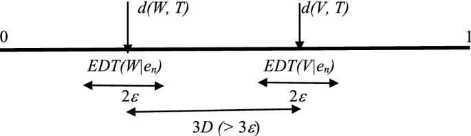
  we may now conclude

• (4) $Prob_{{\underline {t} }} [\forall_{\varepsilon : \, D > \varepsilon > 0} \exists_{N \ge 0} \forall_{n \ge N} (EDT(H_{V} |e_{n} ) - EDT(H_{W} |e_{n} ) > \varepsilon ] = {1}$

In sum, if d(W, T) < d(V, T) then with probability 1 EDT(H_W|e_n) < EDT(H_V|e_n) for n → ∞, i.e. Prob_t [lim_{n →∞} (EDT(H_W|e_n) < EDT(H_V|e_n)] = 1.□

References

Carnap, R. (1952). The continuum of inductive methods. University of Chicago Press.
Feller, W. (1968). An introduction to probability theory and its applications. New York: Wiley.
Festa, R. (1993). Optimum inductive methods. A study in inductive probability theory. Bayesian statistics and verisimilitude. (Synthese Library, Vol. 232) Kluwer Academic Publishers.
Hintikka, J. (1966). Two-dimensional continuum of inductive methods. In J. Hintikka & P. Suppes (Eds.), Aspects of inductive logic. (pp. 113–132). North-Holland Publishing Co.
Knopp, K. (1956). Infinite sequences and series. Dover Publications.
Kuipers, T. (1978). Studies in inductive probability and rational expectation. (Synthese Library, Vol. 123)Dordrecht: Reidel.
Kuipers, T. (2000). From instrumentalism to constructive realism. On some relations between confirmation, empirical progress, and truth approximation. (Synthese Library, Vol. 287)Kluwer Academic Publishers.
Kuipers, T. (2019). Nomic truth approximation revisited. (Synthese Library, Vol. 399). Springer Nature.
Niiniluoto, I. (1987). Truthlikeness. (Synthese Library, Vol. 185). Reidel.
Oddie, G. (1986). Likeness to truth. (Vol. 30). University of Western Ontario Series in Philosophy of Science. Dordrecht: Reidel.
Oddie, G. (2016). ‘Truthlikeness’, The Stanford encyclopedia of philosophy (Winter 2016 Edition), Edward N. Zalta (ed.), https://plato.stanford.edu/archives/win2016/entries/truthlikeness/
Zwart, S. (2001). Refined Verisimilitude. (Synthese Library, Vol. 307). Kluwer Academic Publishers.
Acknowledgements
I am very grateful to Ilkka Niiniluoto who presented this paper on my behalf at the CLMPST19-Prague (August 5–10, 2019) on the symposium: Approaching Probabilistic Truths. I could present it myself in Groningen (PCCP) on October 24, 2019. Partly indirectly, I got some useful comments, for which I am very grateful. I am especially very grateful to David Atkinson and Tom Sterkenburg for their stimulating substantial and technical remarks. The formal versions and proofs of Theorem 3 and its two corollaries are due to David. I also want to thank Jan-Willem Romeijn for his diagnostic help. Finally, I like to thank three anonymous referees for their very useful comments.
Author information
Authors and Affiliations
Corresponding author
Additional information
Publisher's Note
Springer Nature remains neutral with regard to jurisdictional claims in published maps and institutional affiliations.
This article is part of the topical collection on Approaching Probabilistic Truths, edited by Theo Kuipers, Ilkka Niiniluoto, and Gustavo Cevolani.