Parsimonious consensus hierarchies, partitions and fuzzy partitioning of a set of hierarchies

Abstract

Methodology is described for fitting a fuzzy partition and a parsimonious consensus hierarchy (ultrametric matrix) to a set of hierarchies of the same set of objects. A model defining a fuzzy partition of a set of hierarchical classifications, with every class of the partition synthesized by a parsimonious consensus hierarchy is described. Each consensus includes an optimal consensus hard partition of objects and all the hierarchical agglomerative aggregations among the clusters of the consensus partition. The performances of the methodology are illustrated by an extended simulation study and applications to real data. A discussion is provided on the new methodology and some interesting future developments are described.

1 Introduction

The analysis of the relationship within a set of objects, characterised by a set of features, can be described by achieving a hard partition of the objects into disjoint classes, with the property that objects in the same class are perceived as similar to one another. Such partitions can be attained from the application of clustering algorithms (Hartigan 1975; Gordon 1999; Bouveyron et al. 2019), or can be provided directly by observers (judges) in the field of marketing, (e.g., for defining customer types), or in psychology (e.g., for identifying "personas", i.e., personality types). It can also be enlightening to obtain "fuzzy partitions", in which an object need not be associated with a single class, but has a set of membership functions that specify the extent to which it is regarded as belonging to each of the classes. Relevant methodology for obtaining fuzzy partitions is described in several seminal papers (Dunn 1973, 1974; Bezdek 1981, 1987).

Often, several different hierarchies of the same set of objects are available and it is useful to consider obtaining a single ’consensus’ which summarizes the information contained in the separate hierarchies. Some reasons for doing this are given below. First, hierarchical classifications may be obtained by application of an agglomerative or divisive algorithm separately to the same set of multivariate objects observed on different occasions using a set of variables forming a three-way data set, or panel data; or be provided by direct assessment of a set of judges, as can occur in psychometric studies (e.g., Rosenberg and Park 1975) or in marketing, where together with a partition also the aggregation of the clusters are given to form a hierarchy. A consensus hierarchy provides a way of simplifying this information and obtaining an overall view of the relationships within the set of objects. In line with the concept of synthesizing data by defining a central value, the consensus can be defined to be the ’closest’ hierarchy to the given set of hierarchies. Second, the results of a cluster analysis are known to depend on various decisions of the researcher made during the course of the investigation, such as the type of measure of pairwise dissimilarity between objects and clusters and the clustering criterion that is used (e.g. agglomerative or divisive). In effect, each decision that is taken involves a model for the clusters that may bias the results of an analysis towards the assumptions of the model. For this reason, investigators often carry out several different analyses of the same set of objects, each implicitly incorporating a different set of assumptions that are considered to be reasonable. A consensus classification may be considered an ’ensemble’ classification estimating the ’true classification’, that is, the classification less likely to be biased towards the models corresponding to the separate analyses and more likely to reflect the underlying structure of the data. Nevertheless, there are several situations in which obtaining a single consensus hierarchy is too simplistic and na$\ddot{\imath }$ve because several differences may be observed among the set given hierarchies and consequently, more than one consensus hierarchy could be required to synthesize the initial hierarchies. This paper addresses the problem of obtaining partitions of the set of hierarchical classification of objects. These will be referred to as primary hierarchies with associated primary ultrametric matrices, knowing that there is a bijection between hierarchies and ultrametric matrices (Johnson 1967). A fuzzy partition of a set of primary hierarchies will be referred to as a secondary fuzzy partition. The aim of the methodology described in this paper is to obtain a secondary fuzzy partition of the set of primary hierarchies into classes with the property that primary hierarchies with a relevant membership degree for the same class are perceived as similar to one another. Each of the classes will have an associated parsimonious consensus hierarchy, which serves as a summary of the set of primary hierarchies belonging to the class. The secondary partition is fuzzy because it can describe some “uncertainties” that occur in the observed set of primary hierarchies and it provides further information: the membership degrees can show for each class which primary hierarchies are more strongly associated with it and which hierarchies have only a loose association. Therefore, each hierarchy contributes to the definition of all classes according to different membership degrees. The consensus hierarchy (tree) is parsimonious, because it limits its internal nodes to a reduced number G (where G is much smaller than the number N of objects). Thus, the parsimonious trees has the property that clusters appearing in excess of K are viewed as very close to each other and perceived as almost indistinguishable and irrelevant in the hierarchy. In addition, the consensus includes the optimal partition into K clusters. Frequently investigators wish to identify this optimal partition in the hierarchy to detect the most relevant classification of its nested partitions.

The remainder of this paper is organized as follows. Section 2 is fully dedicated to the review of the literature; Sect. 3 describes the proposed methodology and its estimation. The performance of the new methodology is tested in an extended simulation study included in Sects. 4 and 5 includes the applications to real datasets. Finally, Sect. 6 gives remarks and considerations on future developments.

2 Notation and theoretical background

The notation and the theoretical background necessary for the reader to follow the new methodology are reported here. First, the notation is given, followed by some background information on parsimonious hierarchy. The theoretical data structure for multivariate objects and dissimilarities examined on different occasions used in this paper is the three-way array.

2.1 Notation

N, J, H, K, G	number of observations (units), variables, occasions, clusters of occasions, clusters of units, respectively;
${\mathcal {I}}\equiv {1,\dots , N}$	the set of indices identifying units;
${\mathcal {J}}\equiv {1,\dots , J}$	the set of indices identifying variables;
${\mathcal {H}}\equiv {1,\dots ,H}$	the set of indices identifying occasions;
${\textbf{X}}=[x_{ijh}]$	($N \times J \times H$) three-way data array (matrix), where value $x_{ijh}$ is the observation on the i-th unit (row), on the j-th variable (column) on the h-th occasion (layer);
$\mu _{hk}$	membership of h-th occasion in the k-th cluster, for $k=1,\dots , K$, for $h=1,\dots ,H$. For a given occasion, the sum of the membership values for all clusters is one; moreover, memberships can be hard, i.e. $\mu _{hk}\in \{0,1\}$, or fuzzy i.e. $\mu _{hk} \in [0, 1]$;
m	the fuzziness parameter or fuzzifier that controls how fuzzy the classes of the partition tend to be;
${\textbf{U}}=[u_{ilh}]$	($N \times N \times H$) three-way ultrametric matrix formed by H ultrametric matrices. Formally, ${\textbf{U}}=[{\textbf{U}}_1, \dots , {\textbf{U}}_H]$, where ${\textbf{U}}_h$ is a $N\times N$ ultrametric matrix, for $h \in {\mathcal {H}}$;
${\textbf{U}}^{*}=[u^{*}_{ilk}]$	($N \times N \times K$) three-way consensus matrix formed by $(2G-1)$-ultrametric matrices. Formally, ${\textbf{U}}^{*}=[{\textbf{U}}^{*}_{1}, \dots , {\textbf{U}}^{*}_{K}]$, where ${\textbf{U}}^*_k$ is a $N\times N$ ($2G-1$)-ultrametric matrix, for $k=1,\dots , K$.

As described in the introduction H primary hierarchies are supposed observed with associated ultrametric matrices ${\textbf{U}}_1, {\textbf{U}}_2, \dots , {\textbf{U}}_H$.

When hierarchies are not directly observed the data array ${\textbf{X}}=[x_{ijh}: i \in {\mathcal {I}}, j \in {\mathcal {J}}, h \in {\mathcal {H}}]$ is supposed given. Note that the three-way array is the data structure used to organize multidimensional phenomena, with J variables measured on the same set of N individuals, in H different occasions. ${\textbf{X}}=[x_{ijh}]$ has three modes: units (rows), variables (columns), and occasions (times, layers). The term ’way’ refers to a dimension of the data, while the word ’mode’ is reserved for the methods or models used to analyze the data (Kroonenberg 2008). Then, a fixed hierarchical clustering algorithm (Gordon 1999) is applied to each dissimilarity matrix ${\textbf{D}}_h$ related to the data matrix ${\textbf{X}}_h,\ h=1,..., H$, by choosing a dissimilarity measure between multivariate objects.

Each hierarchical classification applied on the data matrix ${\varvec{X}}_h$ has associated:

• (i) N-tree ${\varvec{T}}_h = \{\{i\}, (i \in {\mathcal {I}}), I_{1,h}, I_{2,h},\dots ,I_{N-1,h},{\mathcal {I}}\}$ is a set of subsets of ${\mathcal {I}}$, with $I_{l,h}$ the generic l-th subset of ${\mathcal {I}}$ taken in the h-th occasion: ${\mathcal {I}}\in {\varvec{T}}_h$; $\emptyset \notin {\varvec{T}}_h$; $\{i\} \in {\varvec{T}}_h$; if $I_{i,h}, I_{l,h}\in {\varvec{T}}_h \Rightarrow (I_{i,h}\cap I_{l,h}) \in (I_{i,h}, I_{l,h},\emptyset )$. Thus, the N-tree, for the h-th occasion, is given by the N trivial clusters (leaves) $\{i\}$, $(i \in {\mathcal {I}})$ and the $N-1$ clusters of units (internal nodes), obtained by the $N-1$ steps of fusion performed by a hierarchical algorithm (hence, the last cluster is ${\mathcal {I}}$ or the root). Generally, the N-trees are binary, i.e. they have exactly $N-1$ internal nodes and each node has at most two descendants.

• (ii) Hierarchy (Dendrogram) $\varvec{\delta }_h = \{\delta (I_{1,h}), \delta (I_{2,h}),\dots , \delta (I_{N-1,h})\}$ and $\delta (I_{l,h})$ is the value of fusion determining $I_{l,h}$, such that if $\delta (I_{l,h})\le \delta (I_{i,h})$, implies: $I_{l,h} \subseteq I_{i,h}$ if $I_{l,h}\cap I_{i,h} \ne \emptyset$; otherwise $l\le i$ if $I_{l,h}\cap I_{i,h}= \emptyset$.

• (iii) Ultrametric matrix ${\textbf{U}}_h=[u_{ilh}], u_{iph}\le \max (u_{ilh},u_{plh}) \forall \ (i,l,p) \in {\mathcal {I}}, h\in {\mathcal {H}}$.

From the H given ultrametric matrices, K parsimonious consensus dendrograms, i.e. K $(2G-1)$-ultrametric matrices, summarizing the original H hierarchies will be identified. Each $(2G-1)$-ultrametric matrix, is a square N dimensional matrix with elements satisfying ultrametric inequalities and with off-diagonal elements that can assume one of at most $(2G-1)$ positive different values.

It is now necessary to introduce the model used to obtain a parsimonious tree, associated to a $(2G-1)$-ultrametric matrix.

2.2 Well-structured partition (WSP)

A partition of objects into G clusters has two main characteristics: the isolation between clusters and the heterogeneity within clusters. Vichi (2008) proposed to model a dissimilarity matrix by three matrices: the diagonal matrix $_{W}{\textbf{D}}_k=[_{W}d_{gg}^k > 0: \ _{W}d_{gt}^k = 0, g, t = 1, \dots ,G,\ (g \ne t)],$ the squared matrix $_{B}{\textbf{D}}_k=[_{B}d_{gt}^k >0: \ _{B}d_{gg}^k =0, t, g=1,\dots , G,\ (t\ne g)]$ and the membership matrix ${\textbf{M}}_k=[m_{ig}^k: m_{ig}^k \in \{0,1\}\ \text {for } i=1, \dots , N, g=1, \dots , G, \text {and} \sum _{g=1}^G m_{ig}=1\ \forall \ i=1,\dots , N]$, modelling heterogeneity within clusters, isolation between clusters and the partition into G classes, respectively. Thus, the classification matrix identifying a partition is

$$\begin{aligned} {\textbf{U}}^{*}_k = {\textbf{M}}_k(_{B}{\textbf{D}}_k){\textbf{M}}^{'}_k+ {\textbf{M}}_k(_{W}{\textbf{D}}_k){\textbf{M}}^{'}_k- \text {diag}({\textbf{M}}_k(_{W}{\textbf{D}}_k){\textbf{M}}^{'}_k),\nonumber \\ \end{aligned}$$

(1)

In order to obtain a Well-Structured Partion (Rubin 1967), Equation (1) is subject to the constraint

$$\begin{aligned} {} \max \{ _{W}d_{gg}^k: g=1, \dots , G\} \le \min \{ _{B}d_{gt}^k: t, g=1,\dots , G,\ (g\ne t)\}\nonumber \\ \end{aligned}$$

(2)

In other words, dissimilarities within clusters must be smaller than the dissimilarities between clusters. For the sake of brevity, the matrix form of constraint (2) will be used in the rest of the paper, i.e.

$$\begin{aligned} _{B}{\textbf{D}}_k >\ _{W}{\textbf{D}}_k. \end{aligned}$$

(3)

2.3 Parsimonious hierarchies

When matrix $_{B}{\textbf{D}}_k$ is an ultrametric matrix of order G, then ${\textbf{U}}^{*}_{k}$ is a square $(2G-1)$-ultrametric matrix of order N, with off-diagonal elements that can assume one of at most $(2G -1)$ different values: $0 <\ _{W}d_{gg}^k\le \ _{B}d_{gt}^k (g, t = 1,\dots , G;\ g \ne t)$.

More formally: ${\textbf{U}}^{*}_{k} = [u^{k*}_{il}], u^{k*}_{ii} = 0, u^{k*}_{il} \ge 0, u^{k*}_{il} = u^{k*}_{li}, u^{k*}_{il} \le \max (u^{k*}_{ir}, u^{k*}_{lr} )\ \forall \ (i, l, r)$; furthermore $u^{k*}_{il} \in \{0,\ _{W}d_{gg}^k,\ _{B}d_{gt}^k\}$, with $0 <\ _{W}d_{gg}^k \le \ _{B}d_{gt}^k\ \forall (g, t: g \ne t)$.

There exists a bijection between ultrametric matrices ${\textbf{U}}_h$ and dendrograms (hierarchies), which has been proved by Johnson (1967). Thus, H ultrametric matrices are associated with a set of H dendrograms representing the primary hierarchies $\Delta =[\varvec{\delta }_1, \varvec{\delta }_2, \dots , \varvec{\delta }_H]$.

To clearly show what is meant by parsimonious hierarchy, in the following we consider a $(2G-1)$ dendrogram when $G=5$ and also its corresponding $_{B}{\textbf{D}}$ and $_{W}{\textbf{D}}$ matrices.

Fig. 1

Representation of a $(2G - 1)$-dendrogram when $G= 5$. A 9-dendrogram is shown; the first five clusters ($C_1,\dots ,C_5$) form a partition; clusters $C_6 = \{C_1,C_3\},C_7 =\{C_2,C_4\},C_8 =\{C_6,C_7\},C_9 =\{C_5,C_8\}$, specify the hierarchical structure of the partition

Clearly, the parsimonious dendrogram (PD) displayed in Fig. 1 is associated with a parsimonious hierarchy. Moreover, it is worth noting that the associated isolation and heterogeneity matrices displayed in Table 1 have the following characteristics: matrix $_{W}{\textbf{D}}$ is a diagonal matrix with positive entries on the main diagonal, the matrix $_{B}{\textbf{D}}$ is an ultrametric matrix, and the WSP constraint (2 or 3) holds, with the maximum value of $_{W}{\textbf{D}}$, i.e. 5 being smaller than the minimum value of matrix $_{B}{\textbf{D}}$, i.e. 8.5.

3 Fuzzy partition of hierarchies and their parsimonious consensus dendrograms

The methodology proposed in this paper aims to find a fuzzy partition in K classes of the primary hierarchies with $(2G-1)$-ultrametric consensuses (parsimonious trees) for each class of the partition.

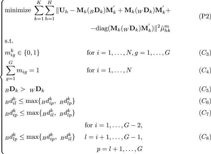
In order to achieve this goal the following optimization problem has to be solved w.r.t. ${\textbf{M}}_k,\ _{B}{\textbf{D}}_k,\ _{W}{\textbf{D}}_k$, and $\mu _{hk}^{m}$,

Table 1 Matrices of isolation between clusters ($_{B}{\textbf{D}}$) and heterogeneity with clusters ($_{W}{\textbf{D}}$)

Constraints $C_{1}$ and $C_{2}$ guarantee that the set of ultrametric matrices ${\textbf{U}}_1, {\textbf{U}}_2, \dots , {\textbf{U}}_H$ is partitioned in a fuzzy way, i.e., into K classes: each ultrametric matrix belongs to the k-th class with the h-th membership $\mu _{hk}$. Constraints $C_{3}$, $C_{4}$ and $C_{5}$ are needed to guarantee that the partition is well-structured. Finally, the last triplet of constraints, i.e. constraints $C_{6}$, $C_{7}$ and $C_{8}$, guarantees that the matrix $_B{\textbf{D}}$ is ultrametric. The whole set of constraints in P1 allows us to obtain a fuzzy partition of the primary hierarchies into K classes, by identifying K parsimonious ultrametric matrices ${\textbf{U}}^*_k$: in this way, each consensus is a $(2G-1)$-ultrametric matrix, and therefore has a parsimonious tree associated with it. The reader can see that if the last triplet of constraints, i.e. constraints $C_{6}$, $C_{7}$ and $C_{8}$, is ignored, then the K consensus matrices are matrices that identify just a well-structured partition and not a parsimonious hierarchy. Finally, the fuzziness of the partition is controlled by the parameter m, named fuzzifier. In particular, when $m \xrightarrow []{} 1$ the partition tends to become hard, i.e. the membership degrees tend to be either 0 or 1; for $m \xrightarrow []{} \infty$ membership tend to be constant and equal to 1/K.

Therefore, problem (P1) can be used in order to solve the following sub-problems:

• (P1.a) Given H primary hierarchies, obtain a fuzzy secondary partition of the primary hierarchies, and for each class of the secondary partition identify a consensus well-structured partition. This problem consists of solving P1 subject to constraints $C_{1}$–$C_{5}$.

• (P1.b) Given H primary hierarchies, obtain a fuzzy secondary partition of the primary hierarchies and for each class of the secondary partition identify a consensus hierarchy with a parsimonious structure. This problem consists of solving P1 subject to constraints $C_{1}$–$C_{8}$.

• (P1.c) Given a single hierarchy (dendrogram), find the closest well-structured partition. If the hierarchy is not initially given, i.e. if a dissimilarity matrix is given, then its corresponding hierarchy or ultrametric matrix can be obtained by applying UPGMA, or any other hierarchical clustering algorithm, to the dissimilarity matrix. This problem consists of solving P1 subject to constraints $C_{1}$–$C_{5}$ when $H=1$ and $K=1$.

• (P1.d) Given a single hierarchy (dendrogram), find the closest parsimonious dendrogram. If the hierarchy is not initially given, i.e. if a dissimilarity matrix is given, then its corresponding hierarchy or ultrametric matrix can be obtained by applying UPGMA, or any other hierarchical clustering algorithm, to the dissimilarity matrix. This problem consists of solving P1 subject to constraints $C_{1}$–$C_{8}$ when $H=1$ and $K=1$.

3.1 Least-squares estimation

In order to implement (P1), it is worth noting that it can be decomposed into two alternating minimization sub-problems:

• (A) the partial minimization of the objective function of (P1) with respect to centroid matrices when these are the parsimonious hierarchies (1). i.e., ${\textbf{U}}^*_k$, and ${\hat{\mu }}_{hk}$ is given.

  

  The solution of this sub-probem (A) can be found by using the Sequential Quadratic Programming (SQP) algorithm (Powell 1983). It is worth noting that the unconstrained least square solution of (P2) is given by ${\bar{\textbf{U}}}_k, \text {for}\ k=1, \dots , K$, where

  $$\begin{aligned} {\bar{\textbf{U}}}_{k}=\frac{1}{\sum _{h=1}^H {\hat{\mu }}^{m}_{hk} }\sum _{h=1}^H{\hat{\mu }}^{m}_{hk}{\textbf{U}}_h \end{aligned}$$

  (4)

  is the weighted arithmetic mean matrix of ${\textbf{U}}_h$, for $h=1, \dots , H$, weighted by ${\hat{\mu }}_{hk}^m$. Typically, matrices ${\bar{\textbf{U}}}_{k}$ are not (2G-1)-ultrametrics. However, only a few iterations are needed for the SQP algorithm to run, if the problem (P2) takes as initial values the matrices ${\bar{\textbf{U}}}_{k}$. For this reason, the following problem is minimized with respect to ${\textbf{U}}^{*}_k$:

  

  by using SQP. An alternative way to optimize (P3) is to solve problem (P3), by using a coordinate descent algorithm where in the step of computing $_BD_k$ the UPGMA algorithm is applied on the matrix $_BD_k$, since UPGMA is known to find an optimal LS ultrametric transformation of $_BD_k$. In this way, the WSP model (model 1) is solved subject to the ultrametricity constraint of the matrix $_{B}{\textbf{D}}$ (i.e. constraints $C_{6}$, $C_{7}$, $C_{8}$) on matrices ${\bar{\textbf{U}}}_k,\ \text {for}\ k=1, \dots , K$ to obtain the corresponding parsimonious ultrametric matrix. In practice, (P3) transforms the dissimilarity matrix ${\bar{\textbf{U}}}_k$ into the closest $(2G-1)$-ultrametric matrix.

• (B) the partial minimization of the objective function of (P2) with respect to the fuzzy partition $[\mu _{hk}]$ when ${\hat{\textbf{U}}}^*_k$ is given

  

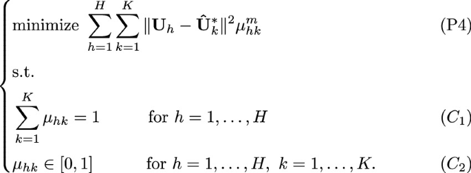
  The minimization of this sub-problem (B) is obtained by solving it by means of the first-order conditions for stationarity. In fact, the stationary point can be found by considering the Lagrangian function

  $$\begin{aligned} \sum _{h=1}^H\sum _{k=1}^{K} \left\| {\textbf{U}}_{h}-{\textbf{U}}^{*}_{k}\right\| ^2 \mu _{hk}^m + \sum _{i=1}^n \lambda _k[\sum _{k=1}^K \mu _{hk}-1], \end{aligned}$$

  (5)

  where the solution with respect to $\mu _{hk}$ is

  $$\begin{aligned} \mu _{hk}=\frac{1}{\sum _{j=1}^K\big (c_{hk}/c_{hj} \big )^{\frac{2}{m-1}}}, \quad \text {for}, h=1, \dots , H, k=1, \dots , K.\nonumber \\ \end{aligned}$$

  (6)

  where $c_{lp}=tr[({\textbf{U}}_{l}-{\hat{\textbf{U}}}^{*}_{p})'({\textbf{U}}_{l}-{\hat{\textbf{U}}}^{*}_{p})].$

After the solution of the two sub-problems (A) and (B) the objective function generally reduces w.r.t. the previous iteration, or at least does not increase. Since it is bounded below by zero, after some iterations the algorithm stops to a stationary point that is not guaranteed to be the global minimum of the problem. For this reason, the algorithm is recommended to be run from several initial starting points to improve the chance of identifying the global optimal solution. The steps of the algorithm can now be formally presented.

ALGORITHM for (P1):

• 0. Initialization Set $t=0$; $\epsilon >0$ convergence constant; and randomly generate the membership degree matrix $[\mu _{hk}]$, with $k=1, \dots , K,\ h=1, \dots H$ from a uniform distribution and make it row-stochastic.

• 1. Do $t=t+1$

• 2. $\underline{\hbox {Given }[{\hat{\mu }}_{hk}], \hbox {solve sub-problem} (A) \hbox {with SQP algorithm}}$ or considering the following steps:

  • (a) Compute ${\bar{\textbf{U}}}_k,\ \text {for } k=1, \dots , K$ as follows:

    $$\begin{aligned} {\bar{\textbf{U}}}_{k}=\frac{1}{\sum _{h=1}^H {\hat{\mu }}^{*}_{hk} }\sum _{h=1}^H{\hat{\mu }}^{*}_{hk}{\textbf{U}}_h \end{aligned}$$

    (7)

  • (b) Solve problem (P3) as follows. For sake of simplicity, we let F be the objective function of problem (P3), namely:

    $$\begin{aligned}&F(_{B}{\textbf{D}}_k, _{W}{\textbf{D}}_k, {\textbf{M}})=\sum \limits _{k=1}^K\Vert {\bar{\textbf{U}}}_k-{\textbf{M}}_k(_{B}{\textbf{D}}_k){\textbf{M}}^{'}_k\nonumber \\&\quad + {\textbf{M}}_k(_{W}{\textbf{D}}_k){\textbf{M}}^{'}_k + \\ {}&\quad - \text {diag}({\textbf{M}}_k(_{W}{\textbf{D}}_k){\textbf{M}}^{'}_k)\Vert ^2 \sum \limits _{h=1}^{H}{\hat{\mu }}_{hk}^{m} \nonumber \end{aligned}$$

    (8)

    It is worth noting that when minimizing (8) w.r.t. $_{B}{\textbf{D}}_k$, $_{W}{\textbf{D}}_k$ and ${\textbf{M}}_k$, ${\hat{\mu }}_{hk}$ is fixed (constant) and therefore only

    $$\begin{aligned}&F(_{B}{\textbf{D}}_k, _{W}{\textbf{D}}_k, {\textbf{M}})=\sum \limits _{k=1}^K\Vert {\bar{\textbf{U}}}_k-{\textbf{M}}_k(_{B}{\textbf{D}}_k){\textbf{M}}^{'}_k\nonumber \\&\quad + {\textbf{M}}_k(_{W}{\textbf{D}}_k){\textbf{M}}^{'}_k +\\ {}&\quad - \text {diag}({\textbf{M}}_k(_{W}{\textbf{D}}_k){\textbf{M}}^{'}_k)\Vert ^2\nonumber \end{aligned}$$

    (9)

    will be minimized w.r.t. $_{B}{\textbf{D}}_k$, $_{W}{\textbf{D}}_k$ and ${\textbf{M}}_k$.

    • (i) Fixing $\hat{{\textbf{M}}}_k$, differentiate the objective function of (P3) (Eq. 9) w.r.t. $_{W}{\textbf{D}}_k$ and equate to zero. The solution $_{W}\hat{{\textbf{D}}}_k$ will have as generic element on the main diagonal:

      $$\begin{aligned} \hat{_{W}d_{gg}^k}=&{} \frac{\sum _{i=1}^n\sum _{l=1, i\ne l}^n\bar{{{\textbf {U}}}}_{il}^k{\hat{m}}_{ig}^k{\hat{m}}_{lg}^k}{\sum _{i=1}^n\sum _{l=1, i\ne l}^n{\hat{m}}_{ig}^k{\hat{m}}_{lg}^k}\quad \quad (g=1, \dots , G);\nonumber \\ \end{aligned}$$

      (10)

    • (ii) Fixing $\hat{{\textbf{M}}}_k$, differentiate the objective function of (P3) (Eq. 9) w.r.t. $_{B}{\textbf{D}}_k$ and equate to zero. The solution $_{B}\hat{{\textbf{D}}}_k$ will have as generic element:

      $$\begin{aligned} \hat{_{B}{d}_{gf}^k}= {} \frac{\sum _{i=1}^n\sum _{l=1, i\ne l}^n\bar{{{\textbf {U}}}}_{il}^k{\hat{m}}_{ig}^k{\hat{m}}_{lf}^k}{\sum _{i=1}^n\sum _{l=1}^n{\hat{m}}_{ig}^k{\hat{m}}_{lf}^k}\ \hspace{0.7cm} (g,f=1, \dots , G);\nonumber \\ \end{aligned}$$

      (11)

    • (iii) Fixing $_{W}\hat{{\textbf{D}}}_k$ and $_{B}\hat{{\textbf{D}}}_k$, minimize the objective function of (P3) (Eq. 9) w.r.t. ${\textbf{M}}_k$. The minimization is done row by row, namely minimizing the objective function w.r.t. row i of ${\textbf{M}}_k$ (${\textbf{m}}_i^k$), fixing the other rows of ${\textbf{M}}_k$; formally the minimization will be done considering ${\textbf{M}}_k=[\hat{{\textbf{m}}}_1^k, \hat{{\textbf{m}}}_2^k, \dots , {\textbf{m}}_i^k, \dots , \hat{{\textbf{m}}}_n^k]^\prime$. Therefore, unit i belongs to the gth class, $m_{ig}^k=1$, if the objective function of (P3) reaches its minimum compared to the situations where unit i is assigned to any other class $v=1, \dots , G,\ v\ne g$. Otherwise, unit i does not belong to class g, i.e. $m_{ig}^k=0$. Formally, for each $i=1, \dots , n$:

      $$\begin{aligned}{} & {} {\hat{m}}_{ig}^k=1,\ \text {if}\ F(_{B}{\textbf{D}}_k, _{W}{\textbf{D}}_k, [\hat{{\textbf{m}}}_1^k, \hat{{\textbf{m}}}_2^k, \dots , \\{} & {} \quad {\textbf{m}}_i^k={\textbf{i}}_g, \dots , \hat{{\textbf{m}}}_n^k]^\prime )= \\{} & {} \quad =\min \{F(_{B}{\textbf{D}}_k, _{W}{\textbf{D}}_k, [\hat{{\textbf{m}}}_1^k, \hat{{\textbf{m}}}_2^k, \dots ,\\{} & {} \quad {\textbf{m}}_i^k={\textbf{i}}_f, \dots , \hat{{\textbf{m}}}_n^k]^\prime ):\\{} & {} \quad f=1, \dots , G\ (f\ne g)\}, \\{} & {} \quad {\hat{m}}_{ig}^k=0,\ \text {otherwise,} \end{aligned}$$

      where ${\textbf{i}}_f$ is the fth row of the identity matrix of order G.

    The proofs of the aforementioned estimates are given by Vichi (2008).

• 3. $\underline{\hbox {Given }\hat{{\textbf{U}}}, \hbox {solve sub-problem } (B)}$ The solution of (P4) is given by:

  $$\begin{aligned} \mu _{hk}= & {} \frac{1}{\sum _{j=1}^K\big (c_{hk}/c_{hj} \big )^{\frac{2}{m-1}}}, \hspace{1cm} \text {for}, h\nonumber \\= & {} 1, \dots , H, k=1, \dots , K. \end{aligned}$$

  (12)

  where $c_{lp}=tr[({\textbf{U}}_{l}-{\hat{\textbf{U}}}^{(t)}_{p})'({\textbf{U}}_{l}-{\hat{\textbf{U}}}^{(t)}_{p})].$

• 4. Stopping Rule Repeat steps 1–3 until the difference between the objective function at iteration t and the objective function at iteration $t-1$ is greater than $\epsilon$.

4 Simulation study

Table 2 Local minima occurrences ($\%$)

Fig. 2

Consensus parsimonious dendrograms (hard assignment experiment)

To assess the performance of the proposed methodology, an extended simulation study has been developed. It consists mainly of two experiments. The former aims to assess whether the proposed methodology is able to recognize the underlying generated hard partition; the latter studies the performance of the proposed methodology in recognizing the underlying generated fuzzy partition. The simulation is organized in the two above briefly described experiments by considering two levels of errors in the data generation process. For each experiment and error level 200 three-way ultrametric matrices have been generated for a total of 800 samples. Details are provided in the corresponding Sects. 4.1 and 4.2. In addition, 200 three-way ultrametric matrices have been generated to study how to avoid local minima in the final solution of the algorithm.

Clearly, since the partitioning problem of a set of multivariate objects is an NP-hard problem (Křivánek and Morávek 1986), there is no guarantee that the new methodology finds a global optimum; indeed, it is possible that the obtained minimum is just a local one. For this reason, the algorithm for each data set is run by using several randomly generated partitions (briefly, "random starts") and the best solution is retained in order to increase the chance of identifying the global minimum solution. More specifically, the correct choice of the number of random starts has been decided by running an experiment, using a high level of error in the generated ultrametric matrices (see Sect. 4.1). The new algorithm was run by letting the number of random starts be 1, 5, 10, 20, 30, and 40. Then, the percentage of the final solutions ending in a local minimum has been computed. Table 2 reports the local minima occurrence (percentage), as the number of random starts increases. It has to be noted that when the number of random starts is set equal to 10, local minima do not occur. Thus, the number of random starts for the whole simulation study was set $RndStarts=10$.

Table 3 Summary statistics (Experiment under a hard assignment with low and high errors)

From Table 2 it can be observed that even with only 1 random start the performance of the algorithm is good, with only $20\%$ local minima occurrences. When 5 random starts are used, the percentage of local minima strongly decreases ($5\%$), thus identifying the global minimum in $95\%$ of cases.

The results of the simulation studies are analyzed by considering several external validity indices to compare the obtained partition with the true one. Adjusted Rand Index (ARI, by Hubert and Arabie (1985)), fuzzy Adjusted Rand Index (Fuzzy ARI, by Campello (2007) and fuzzy Rand Index (Fuzzy RI, by Campello (2007)) have been used. In addition, the Normalized Root Mean Square Error (NRMSE) has been used to compare the obtained consensus matrices with the true ones. Finally, the Mean Membership Matrices are computed to assess whether the methodology is able to recognize the fuzzy or hard assignment: these matrices are obtained by averaging all the membership matrices resulting from each run of the algorithm after optimally permuting their columns in order to avoid the label switching problem.

4.1 First simulation: hard assignment experiment

The first simulation has been developed by considering four $(2G-1)$-ultrametric matrices, with $G=4$. Each of these matrices is associated with a parsimonious dendrogram, as shown in Fig. 2, where the 4 clusters $(c_{1} - c_{4})$ are clearly visible.

Those four $(2G-1)$-ultrametric matrices (${\textbf{U}}^*_k, \ k=1\, \dots , 4$) are used to generate the $H=12$ starting ultrametric matrices (primary hierarchies) (${\textbf{U}}_h,\ h=1, \dots , 12$). In fact, from each ${\textbf{U}}^*_k, \ k=1, \dots , 4$, three different ultrametric matrices are generated by adding a symmetric error matrix to ${\textbf{U}}^*_k$ and forcing the resulting dissimilarity matrix to be ultrametric, by using an average linkage method (UPGMA). Thus, a total of $H=12$ ultrametric matrices are obtained and given as input to the algorithm to recognize the hard assignment, since each of the H ultrametric matrices is associated with the single consensus matrix. The algorithm returns as output not only the obtained secondary partition, but also the parsimonious hierarchy associated with each class of the partition.

Table 4 Mean membership matrices. Experiment under a hard assignment with low and high error

It has to be noted that two levels of errors are considered. A low error should guarantee that the algorithm works in optimal conditions and it should always be able to find the global optimum solution with an ARI always equal to 1. In other words, the algorithm always detects the true (secondary) partition. The high error should identify a strongly biased situation, where the algorithm is able to recognize the true (secondary) partition in the majority of cases.

Table 3 reports the corresponding summary statistics of the performance aforementioned indicators. Particularly, both the mean and the median of the indices regarding 200 iterations are shown. The NRMSE is reported with three different statistics: indeed, in each iteration K NRMSE are computed, each of those measuring the difference between the k-th resulting ultrametric and the k-th original true one; then, the mean, the median and the maximum values are computed.

When using low error, the algorithm performed very well. Indeed, values of ARI, fuzzy ARI and fuzzy RI are close to 1, while values of NRMSE are quite low (Table 3). When using high error, the methodology detects only few times the true partition and low values of ARI, Fuzzy ARI and Fuzzy RI are shown in Table 3. The percentage of ARI equal to one, is $62\%$, as hypothesised from a high level of error. In addition, the values of the NRMSE are significantly larger than zero, meaning that the true parsimonious consensus dendrograms are not perfectly detected.

Moreover, the methodology is able to recognize the underlying hard secondary partition of the ultrametric matrices (primary hiearchies). Indeed, the membership value of each ultrametric matrix to the corresponding cluster is frequently close to 1. The mean membership matrix obtained averaging the 200 obtained matrices is reported in Table  4. Results confirm that when using low error the membership is always larger than 0.8 as expected (Table 4(a)). When using high error, the true partition is still detected, but the highest value (indicating the strongest membership) is about 0.5 (Table  4(b)).

Fig. 3

Consensus parsimonious dendrograms (fuzzy assignment experiment)

Table 5 Summary statistics (Experiment under a fuzzy assignment with low and high errors)

Table 6 Mean membership matrices: experiment under a fuzzy assignment with high error

4.2 Second simulation: fuzzy assignment experiment

The second simulation has been developed by considering two $(2G-1)$-ultrametric matrices, with $G=5$. The associated parsimonious dendrograms are shown in Fig. 3.

Those $K=2$ $(2G-1)$-ultrametric matrices (${\textbf{U}}^*_k, \ k=1\, \dots , 2$) are used to generate the $H=9$ starting ultrametric matrices (primary hierarchies) (${\textbf{U}}_h,\ h=1, \dots , 9$) under a fuzzy assignment scenario. Specifically, from each ${\textbf{U}}^*_k, \ k=1, \dots , K$, three different ultrametric matrices are generated by adding a symmetric error matrix to ${\textbf{U}}^*_k$ and forcing the resulting dissimilarity matrix to be ultrametric, by using an averaging linkage method (UPGMA). Thus, 6 ultrametric matrices are generated and expected to be hardly associated to the corresponding cluster, being themselves generated by one consensus matrix. Moreover, an additional 3 ultrametric matrices are generated by averaging the two consensus matrices, and then adding a symmetric error term, and forcing the resulting matrix to be ultrametric by UPGMA. In this way, the last three ultrametric matrices are expected to be softly associated with both clusters, being themselves generated by a linear combination of the two consensus parsimonious ultrametric matrices.

Therefore, a total of $H=9$ ultrametric matrices are obtained and given as input to the algorithm in order to recognize the fuzzy assignment. The algorithm returns as output not only the obtained secondary partition but also the parsimonious hierarchy associated with each class of the partition.

It has to be noted that also in this case two levels of errors are considered. A low error guarantees that the partition is always detected and therefore all the ARI are equal to 1, while a high error masks the true partition, but still the algorithm detects the partition in the majority of cases.

For the results, we expect that the algorithm almost hardly assigns the first six ultrametric matrices (primary hierarchies) to the corresponding cluster and softly assigns the last three ultrametric matrices (primary hierarchies) to both the clusters. We ran the experiment with both low and high error levels. The results are shown in Table 5, which reports the main statistics of interest and also the percentage of fuzziness detection, i.e. the proportion of occurrences in which the methodology is able to recognize that the last three ultrametric matrices are generated by both the consensuses. When using low error, the percentage of ARI equal to 1 is $100\%$. When the level of error is high, the percentage of ARI exactly equal to 1 is 62$\%$.

From Table 5, we notice that the methodology is able to recognize the underlying partition. For both errors, the mean values of Fuzzy ARI and Fuzzy RI are about 0.5. Clearly, when low error is used, the performance is slightly better. Moreover, the NRMSE are significantly larger than zero, showing differences between generated and obtained consensus parsimonious matrices. In addition, we notice that the proportion of occurrences in which the methodology is able to recognize the fuzzy nature of the last three ultrametric matrices is 1, meaning that the methodology always softly assigns those matrices to both the clusters, regardless the level of error used.

It is worth observing that the new methodology is able to recognize the fuzzy nature of the last three ultrametric matrices (primary hierarchies) and also that the first six are generated by just one consensus matrix. Table 6 shows the mean membership matrix, highlighting that for the first 6 ultrametric matrices the highest membership value is close to 0.9; instead, for the last three ultrametric matrices, both memberships are approximately close to 0.5, meaning that those matrices are softly assigned to both clusters, as expected.

5 Real applications

In the following, two applications to real data are analyzed. The former consists of applying the methodology to the zoo dataset (UCI repository) and refers to problem (P1.d): given a dendrogram, find the closest Least-Square parsimonious dendrogram. The latter consists of applying the methodology to the girls’ growth curves dataset (Sempé and Médico-Sociale 1987) and refers to problem (P1.b): given a set of primary hierarchies, find a fuzzy secondary partition of them, and within each class of the secondary partition, identify a consensus parsimonious dendrogram. Details on the dataset descriptions and on the results of the analyses are provided below.

5.1 Zoo data

For the zoological dataset (dowloaded from the UCI Machine Learning Repository and donated by Richard Forsyth’s) the problem will be reduced in finding the closest parsimonious dendrogram to a given one.

Fig. 4

Original (a) and parsimonious (b) dendrograms (zoo dataset)

The dataset consists of 101 observations (animals) and 18 variables; more in detail, 15 variables are binary, highlighting in each animal the presence/absence of hair, feathers, eggs, milk, airbone, aquatic, predator, toothed, backbone, breathes, venomous, fins, tail, domestic, catsize; one variable is categorical and refers to the number of legs of each animal; one variable refers to the animal name; finally, the last variable is a class attribute, providing the animals’ taxonomy in seven classes: mammals, birds, reptiles, fishes, amphibians, insects, and invertebrates. The whole dataset does not contain any missing value.

For the application, we used the 15 binary variables only. From the units-by-variables data matrix, the dissimilarity matrix ${\textbf{D}}_1$ of dimension $101\times 101$ was obtained by computing the squared Euclidean distance between each pair of units. Then, given ${\textbf{D}}_1$, its closest ultrametric matrix ${\textbf{U}}_1$ was found by applying the UPGMA algorithm on ${\textbf{D}}_1$. Finally, the proposed algorithm, applied on ${\textbf{U}}_1$ by setting $G=7$ and using 100 random starts, found a unique ($K=1$) consensus parsimonious dendrogram. In Fig. 4a and b, the starting ultrametric matrix and the closest parsimonious dendrogram are shown, respectively. As it is shown in Fig. 4a, the partition of the animals in $G=7$ clusters with cutoff level 1.94 is not clearly identifiable, because by moving the cutoff level slightly up (level 1.95) or down (level 1.91) the number of clusters of the partition varies from 6 to 8. Thus, there is an uncertainty in the identification of the cutting level. In practice, the visual inspection of the dendrogram does not show a clear distinction between the partitions on 6, 7, or 8 clusters. This situation does not occur in Fig. 4b, where the $G=7$ classes are clearly visible and identifiable by the investigator. In this case, the taxonomy of animals (mammals, birds, reptiles, fishes, amphibians, insects, and invertebrates) is clearly identified and their clustering aggregations (such as oviparous vs mammals, non-toothed vs toothed and non-aquatic vs aquatic) can be appreciated.

In order to understand whether the classification taxonomy is recognized, we compared it with the partition of the animals in $G=7$ classes derived from the complete (UPGMA) dendrogram in Fig. 4a and with the partition corresponding to the consensus parsimonious dendrogram in Fig. 4b. The ARI values are equal to 0.796 and 0.853, respectively. Thus, the taxonomy in 7 classes is better recovered by the PD. Therefore, in terms of classification tasks, our proposal performs better than the standard methodology. The confusion matrix between true partition in 7 classes and the one of PD is displayed in Table 7. We observe that most of the animals are correctly classified (bold on the diagonal) and only $13\%$ of animals are misclassified (13 animals out of $n=101$ animals) and are highlighted in italic in the Table 7.

It is worthy to observe that the hierarchical aggregations in PD (in Fig. 4b) have a very clear meaning. For $G=7$, we have: mollusks (aquatic animals of the class ’invertebrates’) ($C_1$), bugs and worm, slug, scorpion (terrestrial animals of the class ’invertebrates’) ($C_2$), birds and tortoile (one animal of class ’reptiles’) ($C_3$), fishes ($C_4$), amphibians and reptiles (all but tortoile) ($C_5$), terrestrial mammals ($C_6$) and finally aquatic mammals (e.g. "dolphin", "platypus", "sealion", "porpoise" and "seal") ($C_7$). Moreover, the parsimonious dendrogram allows the study of all the aggregations of those clusters into wider ones: the first aggregations into wider clusters occur by grouping terrestrial mammals and acquatic mammals ($C_6$ and $C_7$) in the ’mammals’ cluster ($C_6$+$C_7$) thanks to the variable ’acquatic’ and by grouping fishes and amphibians+reptiles ($C_4$ and $C_5$) thanks to the variables related to the presence/absence of ’breath’ and ’fins’; moreover, the partition into 4 clusters is obtained by grouping mollusks and insects ($C_1$ and $C_2$); then, birds ($C_3$) join the cluster with mollusks and bugs ($C_1$+$C_2$) thanks to the variable related to the presence/absence of ’feathers’, ’tails’ and ’backbone’ and thus creating a partition with $G=3$ clusters. Finally, in order to obtain a partition with $G=2$ clusters, thanks to the variable ’toothed’, this new cluster ($C_1$+$C_2$+$C_3$), characterized by all non-toothed and mostly terrestrial animals and with no fins and no hair, is aggregated with the cluster including fishes, amphibians and reptiles ($C_4$+$C_5$), characterized by all toothed animals with no feathers, no hair, mostly aquatic and vertebrates. The obtained cluster ($C_1+C_2+C_3+C_4+C_5$) referring to ’oviperous’ animals and the cluster ($C_7$+$C_8$) referring to the ’mammals’ make up the partition in only two clusters, where the discriminant variable is the one referring to presence/absence of ’milk’.

5.2 Girls’ growth curves

For the second application we use the girls’ growth curves dataset (Sempé and Médico-Sociale 1987), downloaded from the webpage of Prof. P.M Kroonenberg and donated by Prof. M. Sempé. The dataset includes 8 physical measurements of 30 girls collected from 1953 until 1975 during a French auxiological study: particularly, the biometric variables related to physical growth (weight, length, crown-rum length, head circumference, chest circumference, arm, calf, pelvis) are measured yearly in the selected girls, who started the experiment at age 4 and ended the experiment at age 15. The data set is therefore a three-way data array with three modes: the first refers to 30 girls, the second to 8 variables, and the third to 12 years.

Table 7 Confusion matrix: true partition compared to obtained partition of animals of the PD (zoo dataset)

The objective of the analysis is to compute 12 dendrograms (primary hierarchies) and apply our methodology to identify a fuzzy secondary partition of them and within each class of the secondary partition, identify a consensus parsimonious dendrogram. Before applying the new methodology, a preliminary data manipulation is needed, by normalizing the overall dataset with min-max normalization, where the min and the max of variables are over the entire period (4–15 years old). Then, the overall average trends of the 8 observed variables among the 30 girls are shown in Fig. 5. The trends are clearly increasing and it is possible to observe a change in the slope of the growth around age 9–10.

Fig. 5

Average trends of the variables of interests from age 4 until age 15 (girls’ growth curves dataset)

The starting $H=12$ dendrograms (H ultrametric matrices or primary hierarchies) are obtained by considering the H matrices ${\textbf{X}}^N_h,\ h=1,\dots , 12$, where ${\textbf{X}}^N_h$ is the $30\times 8$ normalized data matrix referring to the physical measurements at age h. Then, we obtained the H dissimilarity matrices ${\textbf{D}}_h,\ h=1,\dots , 12$ by computing the Euclidean distance between each pair of units. Finally, in Fig. 6 the dendrograms $\Delta =\{\delta _1, \dots , \delta _{12}\}$ of Ward’s method of hierarchical clustering, computed on matrices ${\textbf{D}}_1, {\textbf{D}}_2,\dots , {\textbf{D}}_{12}$ are from age 4 to age 15 years old.

Fig. 6

Hierarchical clustering of the girls by 8 biometric variables from age 4 until age 15 (girls’ growth curves dataset)

Table 8 Cluster assignment of the original dendrograms to 2 clusters, with the highest membership degree

Given the $H=12$ primary hierarchies, the algorithm is applied on the corresponding ultrametric matrices ${\textbf{U}}_1, \dots , {\textbf{U}}_{12}$, by using 100 random starts and setting $G=3$ and $K=2$, as suggested by Kroonenberg et al. (1987). The algorithm finds a fuzzy partition of the primary hierarchies into $K=2$ clusters and within each class of the secondary partition identifies a consensus parsimonious dendrogram, i.e. a $(2G-1)$-ultrametric matrix, where $G=3$ identifies the number of classes of the girls.

The obtained fuzzy partition is illustrated in Table 8, where for each age of the girls the corresponding cluster and the related membership degree are reported. In particular, we observe that the chronological order is retained, as ages 4–8 belong almost hardly to the first cluster, and ages 11–15 belong almost hardly to the second cluster. In addition, ages 9 and 10 are more softly associated to both clusters, having membership degrees quite fuzzier and closer to one another. This result is interesting and meaningful: indeed, at ages 9 and 10 we observed in Fig. 5 that several curves change their slopes. More generally, it has been shown by many research studies (Breehl and Caban 2021; Farello et al. 2019) that the puberty period for girls starts around age 8 and therefore ages 9 and 10 are exactly when the puberty period is in progress. For this reason, we can conclude that the proposed approach allows us to detect the ages which can be considered as a transitional period in these data.

In addition, the resulting parsimonious consensus dendrograms are shown in Fig. 7, where we can clearly see the aggregations of the girls into $G=3$ clusters and the distinct agglomerations of these clusters.

Fig. 7

Resulting consensus dendrograms, representing hierarchical clustering of girls by 8 biometric variables (girls’ growth curves dataset)

Fig. 8

Solid lines: trends of the dimensions taken from the variables of interest separately per cluster of ages and class of girls. Dotted lines: average trends of the dimensions in the entire period. Title of the subplots are colored with the color of the class of girls in Fig. 7 (girls’ growth curves dataset)

It is worthy to notice that clusters $C_1$, $C_2$ and $C_3$ of girls, identified in the two parsimonious dendrograms, have some common individuals, but also show some differences due to the fact that some girls have changed the pattern of growth from the first period to the second, thus, moving from one cluster to another. In order to better visualize and interpret the results, the hard partition of ages was considered by applying MAP (maximum a posteriori) to the membership degree matrix. This allowed us to have separate plots of the trends of the variables for the two clusters of ages, and the three clusters of girls. For the visualization task and to reduce the amount of trends to be plotted it was decided to plot only the three dimensions identified by Kroonenberg et al. (1987) and named Skeletal Length, Skeletal Width and Stoutness: Skeletal Length is referred to variables length and crown-rump length, Skeletal Width to variables head and pelvis, Stoutness to variables weight, chest, arm and calf. The trends of these dimensions are shown in Fig. 8 (solid lines) separately by cluster of ages and cluster of girls, as well as the average trend of each dimension in that specific period (i.e. cluster of ages) (dotted lines).

From Fig. 8, it is possible to comment on the clusters of girls obtained separately for each cluster of ages. We observe that the trends of the girls who belong to the first cluster between ages 4 and 9 ($C_1$ in the left dendrogram in Fig. 7) are quite far below the average level, meaning that those girls are below average stature, characterized by a less rapid growth and low levels of biometric variables. Girls belonging to the second cluster when they are between 4 and 9 years old ($C_2$ in the left dendrogram in Fig. 7) grow on average: trends are very close to the corresponding average; they can be considered a cluster of average stature girls. Finally, those who belong to the third cluster of girls between ages 4 and 9 ($C_3$ in the left dendrogram in Fig. 7) have trends far above the average ones. This means that those girls are the most robust and tallest ones (above average stature girls). In addition, focusing on the ages 10–15, girls who fall into the first cluster are the ones in the first cluster between ages 4–9 except for unit 3 (as depicted in Fig. 7, cluster $C_1$): their trends have similar behaviour as in the earlier ages, being far below the average; therefore this cluster identifies the below average stature girls. The second cluster of girls being between 10 and 15 years old ($C_2$ in the right dendrogram in Fig. 7) have trends following the average, as happens in the earlier ages, except for Skeletal Length, which is slightly above the average. Therefore, the cluster groups together the average stature girls; it is worth mentioning that unit 3, who falls in the below average stature girls cluster between ages 4 and 9, joins the average stature girls cluster in the next ages’ period, meaning that her biometric variables’ trends returned to the average level. Finally, the third cluster of girls between ages 10–15 ($C_3$ in the right dendrogram in Fig. 7) have similar trends as the earlier ages, thus identifying the above average stature girls.

In conclusion, the analysis allowed us to identify two distinct clusters of ages (one for ages 4–8, one for ages 11–15), except for ages 9–10 which are in the middle of the two, characterizing a transitional period in the girls’ physical growth. In addition, for each cluster of ages a consensus parsimononious dendrogram has been identified. Both of the consensus dendrograms identify three distinct clusters of girls. By analyzing these separately per cluster of ages, we noticed that they correspond to below average stature girls ($C_1$ in Fig. 7), average stature girls ($C_2$ in Fig. 7) and above average stature girls ($C_3$ in Fig. 7); more specifically, considering the entire period, very few girls are always under the average (see clusters $C_1$ of Fig. 7), some girls who were on average during ages 4–9 became above the average in the following ages (see for example unit 7 and 28 move from $C_2$ to $C_3$ in Fig. 7), and some girls who were above the average during ages 4–9 became on average during the next years (see for example unit 5 moves from $C_3$ to $C_2$ in Fig. 7).

6 Conclusion

The new methodology proposed in this paper makes it possible to solve several problems:

• (i) Given H primary hierarchies, obtain a fuzzy secondary partition of the primary hierarchies, and for each class of the secondary partition identify a consensus well-structured partition (where within-cluster distances are all smaller than between-cluster distances). This problem consists of solving simultaneously a fuzzy partitioning problem to identify the secondary partition and K least-squares optimal differences between ultrametric matrices of a cluster of the secondary partition and a consensus well-structured partition that should identify the partition closest to the hierarchies (see the problem (P1.a) in Sect. 3);

• (ii) Given H primary hierarchies, obtain a fuzzy secondary partition of the primary hierarchies, and for each class of the secondary partition identify a consensus parsimonious dendrogram. This problem consists of solving simultaneously a fuzzy partitioning problem to identify the secondary partition and K least-squares optimal differences between a subset of ultrametric matrices and a consensus parsimonious dendrogram (see the problem (P1.b) in Sect. 3);

• (iii) Given a single hierarchy (dendrogram), find the closest well-structured partition. This is a problem frequently considered in hierarchical clustering, where the investigator has to find an optimal partition by the visual inspection of the dendrogram or by means of a specific methodology. This problem consists of solving the problem (i) above when a single dendrogram is observed or computed, and it is necessary to find a single well-structured partition (see the problem (P1.a) with H = 1 and K = 1, in Sect. 3).

• (iv) Given a single hierarchy (dendrogram), find the closest parsimonious dendrogram. This is an evolution of the previous problem (iii) where the investigator wishes to find an optimal partition in G classes in the ultrametric matrix (dendrogram) and the corresponding optimal aggregations from G to 1. This problem consists of solving the problem (ii), when a single dendrogram is observed or computed and it is necessary to find a single consensus parsimonious dendrogram (see the problem (P1.b) with H = 1 and K = 1, in Sect. 3).

For problems (iii) and (iv) if the hierarchy is not initially given, i.e. if a dissimilarity matrix is given, then its corresponding hierarchy or ultrametric matrix can be obtained by applying UPGMA, or any other hierarchical clustering algorithm, to the dissimilarity matrix.

For problems (i) and (ii) a secondary fuzzy partition that allows each dendrogram of the primary partition to belong to all clusters of the secondary partition according to different membership degrees is required. This guarantees great flexibility in the results and their interpretation.

For each class of the fuzzy partition, a consensus hierarchy (dendrogram) is identified. However, several authors have noted that the complete sets of partitions and clusters of the dendrogram are not all used by investigators, even hindering interpretation (Gordon 1999). One approach for resolving this difficulty has involved the construction of a parsimonious dendrogram that contains a limited number of internal nodes. Some information is lost here, but the main features of the data are represented more clearly (Gordon 1999). For this reason, the consensus hierarchy in this paper has a parsimonious structure.

The proposed methodology has been tested in an extended simulation study, where 1000 three-way arrays of ultrametric matrices have been generated. Two scenarios of hard assignment and fuzzy assignment of the primary hierarchies to the consensus hierarchies have been considered. The study showed good results, not only in recovering the underlying true secondary partition but also in identifying consensus parsimonious dendrograms very similar to the original ones.

The methodology has also been applied to real datasets; the results of the analyses show that the proposed methodology is helpful in partitioning the primary hierarchies in a fuzzy manner, by identifying correctly the hierarchies which share characteristics with more than one cluster of the secondary partition: for example, in the application to girls’ growth curves dataset, two periods of contiguous ages are identified and the hierarchies corresponding to two transitional years from one period to the following are reasonably softly assigned to both periods. In addition, for each class (period) of the fuzzy partition, the methodology identifies a consensus parsimonious dendrogram, which really facilitates the interpretation of the aggregation of the girls.

This research work introduces a new methodology in multidimensional data analysis and opens up the possibility to new applications and further developments. For instance, let us consider a scenario where units (or objects) represent a set of countries whose macroeconomic performance is assessed across several years. This assessment involves creating a hierarchy of classes (a dendrogram) for each year, where countries within the same class are seen as similar to one another. Consequently, consensus hierarchies would recognize similar clusters and cluster groupings across different years.

Alternatively, such data might arise from various data-collection methods, like data cards in psychometric studies, or products in marketing analyses. Here, individuals (customers) categorize similar items into clusters they perceive as alike and then combine these clusters to form a hierarchy. Therefore, consensus hierarchy derived from customer-defined hierarchies would identify the closest hierarchy to the ones observed.

However, differences can emerge among the given hierarchies, necessitating more than one consensus hierarchy to summarize the initial hierarchies. For instance, macroeconomic performances of different countries might change following an economic shock after a period of stability. Consequently, the relationships between countries may shift, requiring a different consensus hierarchy for each stable period. In data gathering, individuals might use multiple criteria to categorize items, resulting in different hierarchical relations.

Additionally, our proposal enables the identification of a fuzzy partition of the initial hierarchies and for each class of the fuzzy partition a consensus parsimonious dendrogram. The practical value of this proposal is evident in real datasets, such as hierarchies describing the macroeconomic outlook of countries over several years.

Consider, for example, a scenario where macroeconomic outlook hierarchies for different countries remain relatively stable during a period of stability. In the event of an economic shock, drastic changes occur in the macroeconomic outlook and hierarchical relations among countries. After a subsequent period of stability, new hierarchical relations may emerge among countries. A fuzzy partition can indicate the uncertainty during the shock years by specifying membership degrees for each class.

Moreover, parsimonious consensus hierarchies help highlight relevant groups of countries and their hierarchical aggregations. In marketing product applications, a fuzzy partition allows each customer to belong to multiple clusters, crucial for dealing with diverse personal opinions. Additionally, the parsimonious structure of consensus hierarchies facilitates the identification of key customer groups and their hierarchical arrangements.

References

Bezdek, J.C.: Some non-standard clustering algorithms. In: Develoments in Numerical Ecology. Springer, pp. 225–287 (1987)
Bezdek, J.C.: Pattern Recognition with Fuzzy Objective Function Algorithm. Plenum Press, New York (1981)
Bouveyron, C., Celeux, G., Murphy, T.B., Raftery, A.E.: Model-Based Clustering and Classification for Data Science: with Applications in R, vol. 50. Cambridge University Press, Cambridge (2019)
Breehl, L., Caban, O.: Physiology, puberty. In: StatPearls [Internet]. StatPearls Publishing; (2021)
Campello, R.J.: A fuzzy extension of the Rand index and other related indexes for clustering and classification assessment. Pattern Recogn. Lett. 28(7), 833–841 (2007)
Dunn, J.C.: A fuzzy relative of the ISODATA process and its use in detecting compact well-separated clusters. J. Cybern. 3(3), 32–57 (1973)
Dunn, J.C.: Well-separated clusters and optimal fuzzy partitions. J. Cybern. 4(1), 95–104 (1974)
Farello, G., Altieri, C., Cutini, M., Pozzobon, G., Verrotti, A.: Review of the literature on current changes in the timing of pubertal development and the incomplete forms of early puberty. Front. Pediatr. 7, 147 (2019)
Gordon, A.D.: Classification, 2nd Edition. Chapman & Hall/CRC Monographs on Statistics & Applied Probability. CRC Press (1999). https://books.google.it/books?id=_w5AJtbfEz4C
Hartigan, J.A.: Clustering Algorithms. Wiley, New York (1975)
Hubert, L., Arabie, P.: Comparing partitions. J. Classif. 2(1), 193–218 (1985)
Johnson, S.C.: Hierarchical clustering schemes. Psychometrika 32(3), 241–254 (1967)
Křivánek, M., Morávek, J.: NP-hard problems in hierarchical-tree clustering. Acta Inf. 23(3), 311–323 (1986)
Kroonenberg, P.M., Janssen, J., Marcotorchino, F., Proth, J.: Multivariate and longitudinal data on growing children. Solutions using a three-mode principal component analysis and some comparison results with other approaches. Data analysis The ins and outs of solving real problems, pp. 89–112 (1987)
Kroonenberg, P.M.: Applied Multiway Data Analysis, vol. 702. Wiley, New York (2008)
Powell, M.J.: Variable metric methods for constrained optimization. In: Mathematical programming the state of the art. Springer, pp. 288–311 (1983)
Rosenberg, S., Park, Kim M.: The method of sorting as a data-gathering procedure in multivariate research. Multivar. Behav. Res. 10(4), 489–502 (1975)
Rubin, J.: Optimal classification into groups: an approach for solving the taxonomy problem. J. Theor. Biol. 15(1), 103–144 (1967)
Sempé, M., Médico-Sociale, G.d.: Presentation of the French Auxological Survey. In: Data Analysis. Springer, pp. 3–6 (1987)
Vichi, M.: Fitting semiparametric clustering models to dissimilarity data. Adv. Data Anal. Classif. 2(2), 121–161 (2008)
Funding
Open access funding provided by Università degli Studi di Roma La Sapienza within the CRUI-CARE Agreement.
Author information
Authors and Affiliations
Contributions
I.B., and M.V. contributed to the design and implementation of the research, to the analysis of the results and to the writing of the manuscript.
Corresponding author
Ethics declarations
Conflict on interest
The authors declare no competing interests.
Additional information
Publisher's Note
Springer Nature remains neutral with regard to jurisdictional claims in published maps and institutional affiliations.
Rights and permissions
Open Access This article is licensed under a Creative Commons Attribution 4.0 International License, which permits use, sharing, adaptation, distribution and reproduction in any medium or format, as long as you give appropriate credit to the original author(s) and the source, provide a link to the Creative Commons licence, and indicate if changes were made. The images or other third party material in this article are included in the article’s Creative Commons licence, unless indicated otherwise in a credit line to the material. If material is not included in the article’s Creative Commons licence and your intended use is not permitted by statutory regulation or exceeds the permitted use, you will need to obtain permission directly from the copyright holder. To view a copy of this licence, visit http://creativecommons.org/licenses/by/4.0/.
About this article
Cite this article
Bombelli, I., Vichi, M. Parsimonious consensus hierarchies, partitions and fuzzy partitioning of a set of hierarchies. Stat Comput 34, 114 (2024). https://doi.org/10.1007/s11222-024-10415-7
Received:
Accepted:
Published:
DOI: https://doi.org/10.1007/s11222-024-10415-7