A New View of the Solar Interface Region from the Interface Region Imaging Spectrograph (IRIS)

Abstract

The Interface Region Imaging Spectrograph (IRIS) has been obtaining near- and far-ultraviolet images and spectra of the solar atmosphere since July 2013. IRIS is the highest resolution observatory to provide seamless coverage of spectra and images from the photosphere into the low corona. The unique combination of near- and far-ultraviolet spectra and images at sub-arcsecond resolution and high cadence allows the tracing of mass and energy through the critical interface between the surface and the corona or solar wind. IRIS has enabled research into the fundamental physical processes thought to play a role in the low solar atmosphere such as ion–neutral interactions, magnetic reconnection, the generation, propagation, and dissipation of waves, the acceleration of non-thermal particles, and various small-scale instabilities. IRIS has provided insights into a wide range of phenomena including the discovery of non-thermal particles in coronal nano-flares, the formation and impact of spicules and other jets, resonant absorption and dissipation of Alfvénic waves, energy release and jet-like dynamics associated with braiding of magnetic-field lines, the role of turbulence and the tearing-mode instability in reconnection, the contribution of waves, turbulence, and non-thermal particles in the energy deposition during flares and smaller-scale events such as UV bursts, and the role of flux ropes and various other mechanisms in triggering and driving CMEs. IRIS observations have also been used to elucidate the physical mechanisms driving the solar irradiance that impacts Earth’s upper atmosphere, and the connections between solar and stellar physics. Advances in numerical modeling, inversion codes, and machine-learning techniques have played a key role. With the advent of exciting new instrumentation both on the ground, e.g. the Daniel K. Inouye Solar Telescope (DKIST) and the Atacama Large Millimeter/submillimeter Array (ALMA), and space-based, e.g. the Parker Solar Probe and the Solar Orbiter, we aim to review new insights based on IRIS observations or related modeling, and highlight some of the outstanding challenges.

1 Introduction

The Interface Region Imaging Spectrograph (IRIS) is a NASA Small Explorer consisting of a 20 cm telescope that feeds far (FUV) and near ultraviolet (NUV) light into a high-resolution spectrograph. IRIS obtains spectra and images at unprecedented cadence (down to 1.3 seconds) and resolution both spatially ($0.33^{\prime \prime }$ in the FUV, $0.4^{\prime\prime }$ in the NUV) and spectrally ($2.7~\text{km}\,\text{s}^{-1}$ pixels), allowing flexible rastering of fields of view that cover a large fraction of an active region (De Pontieu et al., 2014b). IRIS was launched in June 2013 and after a two-year prime mission, it is now in the extended-mission phase. IRIS observations continue to provide high-resolution images and spectra of the photosphere, chromosphere, transition region (TR), and corona.

In the almost eight years since launch, IRIS has opened a new window in the complex physics of the solar interface region: a region sandwiched between the solar photosphere and the corona. It is through this region that all of the non-thermal energy that powers the outer solar atmosphere and solar wind is processed and propagated. The interface region includes the chromosphere, transition region, and low corona and is characterized by several physical transitions that render analysis, interpretation, and understanding challenging. The plasma undergoes a transition from partially ionized in the chromosphere and low transition region to fully ionized in the corona. Starting from magnetic-field strengths similar to those observed, numerical models conclude that, apart from sunspots, the plasma-$\beta$ is largely $\ll 1$ at roughly 1000 km above the photosphere and $>1$ below this height (e.g. Hansteen, Carlsson, and Gudiksen, 2007; Hansteen et al., 2015). Thus, outside of sunspots, the plasma dominates the dynamics of the magnetic field in the photosphere; forcing the field into flux concentrations in the downflows of the convective flow pattern, while the magnetic field becomes more dominant with increasing height and is volume filling in the corona. This transition from high to low plasma-$\beta$ leads to a variety of complex physical processes, including wave-mode coupling. When trying to diagnose conditions in the low solar atmosphere, we are limited to remote sensing of the radiation emanating from this region. However, most chromospheric diagnostics are optically thick and require non-LTE radiative transfer modeling to be properly understood. This can complicate the interpretation of some of the IRIS diagnostics significantly. All of these complex issues imply that, in order to obtain a deeper understanding of the dominant physical processes that drive the dynamics and energetics in the interface region, numerical modeling needs to go hand-in-hand with observations. The IRIS science investigation has included a numerical-modeling component from the beginning, and we will thus provide an overview of the most exciting developments in observations as well as modeling of the interface region in what follows below.

The IRIS bandpasses have previously been studied at lower resolution using rockets (Bates et al., 1969; Fredga, 1969; Kohl and Parkinson, 1976; Allen and McAllister, 1978; Morrill and Korendyke, 2008; West et al., 2011; Dere, Bartoe, and Brueckner, 1984; Brekke, 1993), balloons (Lemaire, 1969; Lemaire and Skumanich, 1973; Samain and Lemaire, 1985; Staath and Lemaire, 1995), or spacecraft (Doschek and Feldman, 1977; Bonnet et al., 1978; Woodgate et al., 1980; Roussel-Dupre and Shine, 1982; Billings, Roussel-Dupre, and Francis, 1977; Cohen, 1981; Poland and Tandberg-Hanssen, 1983; Kingston et al., 1982; Hayes and Shine, 1987; Curdt et al., 2001). However, the advances of IRIS in spatial, spectral, and temporal resolution compared to previous missions are large enough that a comparison with results from such missions is less useful. Instead, we will focus on the physical insights that have resulted from IRIS observations, and frame those within the context of what was previously known about the physical mechanisms in this region of the solar atmosphere. Many of the IRIS results were obtained through coordinated observations with a variety of other instruments, including the Atmospheric Imaging Assembly (AIA: Lemen et al., 2012) and the Helioseismic and Magnetic Imager (HMI: Scherrer et al., 2012) onboard the Solar Dynamics Observatory (SDO: Pesnell, Thompson, and Chamberlin, 2012); the Solar Optical Telescope (SOT: Tsuneta et al., 2008), the Extreme-ultraviolet Imaging Spectrometer (EIS: Culhane et al., 2007), and the X-Ray Telescope (XRT: Golub et al., 2007) onboard the Hinode spacecraft¹ (Kosugi et al., 2007); the Solar and Terrestrial Relations Observatory/Sun Earth Connection Coronal and Heliospheric Investigation instrument (STEREO/SECCHI Howard et al., 2008); the Reuven Ramaty High Energy Solar Spectroscopic Imager mission (RHESSI: Lin et al., 2002); the Nuclear Spectroscopic Telescope Array mission (NuSTAR: Harrison et al., 2013); the High Resolution Coronal Imager sounding rocket (Hi-C: Kobayashi et al., 2014); as well as the ground-based Swedish 1 m Solar Telescope (SST: Scharmer et al., 2003), the Goode Solar Telescope at the Big Bear Solar Observatory (BBSO: Goode et al., 2003), the GREGOR telescope (GREGOR: Schmidt et al., 2012), and the Atacama Large Millimeter/submillimeter Array (ALMA) radio telescope. In addition, we will describe outstanding challenges, also in light of the advent of novel instrumentation such as NSF’s 4 m Daniel K. Inouye Solar Telescope (DKIST: Rimmele et al., 2020), the Solar Orbiter (Müller et al., 2020), and Parker Solar Probe (PSP: Fox et al., 2016) missions, as well as advances in numerical modeling.

The data analysis and interpretation of IRIS observations, as with any spectroscopic data, depend on a careful and accurate calibration. A detailed description of the IRIS calibration is provided by Wülser et al. (2018).

This article is divided into several sections that are aligned with the prioritized science goals of the IRIS extended mission: We first discuss the progress made in diagnosing physical conditions from the IRIS observables (Section 2) and briefly describe the numerical models that have been made publicly available as part of the IRIS mission (Section 3). Section 4 focuses on the advances made in understanding the fundamental physical processes that play a role in the interface region. We further discuss the large-scale instability of the solar atmosphere (Section 5) through flares and coronal mass ejections (CMEs). We also cover contributions from IRIS to studies of solar irradiance (Section 6) and the solar-stellar connection (Section 7). We finish with a brief summary (Section 8).

2 Diagnostics

2.1 Photospheric and Chromospheric Lines

The chromosphere is a highly complex, finely structured, and dynamic region in which non-LTE radiative transfer and time-dependent ionization play a major role. Determining the physical parameters in this region has traditionally been a major challenge. Two different approaches have been used to significantly increase the diagnostics power of spectral lines such as Mg ii h (2803 Å), k (2796 Å), and UV triplet (2798.82 Å, 2798.75 Å, 2791.6 Å), or C ii 1334 and 1335 Å.

We outline these two different approaches below:

In the first approach, forward-modeling of synthetic observables from advanced numerical simulations (using the Bifrost code, Gudiksen et al., 2011) has been used to study correlations between physical variables in the chromosphere and properties of the spectral lines (e.g. Doppler shifts, intensity, central reversal). These correlations are described in a series of nine articles and have provided us with new diagnostics that (approximately) map the extensive spectroscopic IRIS observables to physical properties of the low solar atmosphere (see also Carlsson, De Pontieu, and Hansteen, 2019). Here we briefly summarize the results of these studies. The many photospheric lines in the wings of the Mg ii h and k lines in the IRIS NUV passband provide velocity diagnostics over a wide range of heights above the photosphere, through measurements of Doppler shifts of absorption lines (Pereira et al., 2013). Analysis of the line formation of the Mg ii h and k lines has shown that these lines have great diagnostic value for the chromosphere. They form over a wide range of heights and the spectral-line parameters (e.g. Doppler shift and intensity of k2v, k2r, k3, see Figure 1) can be used to estimate physical parameters such as the middle and upper chromospheric velocity, chromospheric velocity gradients, and temperatures in the middle chromosphere (Leenaarts et al., 2013a,b; Pereira et al., 2013). Software is available to determine these spectral parameters in the IRIS tree of SolarSoft (see IRIS data analysis guides for IDL and Python at iris.lmsal.com/analysis.html). Heating in the low chromosphere can be identified from emission in the Mg ii triplet lines (Pereira et al., 2015), while upper chromospheric velocities can be estimated from the C ii lines (Rathore and Carlsson, 2015; Rathore et al., 2015). Velocities in the middle chromosphere can be estimated from Doppler shifts of the C i 1355.8 Å line (Lin, Carlsson, and Leenaarts, 2017). One of the most interesting diagnostics is the O i 1355.6 Å line, which is formed over a wide range of chromospheric heights under optically thin conditions (Lin and Carlsson, 2015). This means that it is uniquely sensitive to non-thermal motions in the chromosphere (through its broadening). In addition, the ratio of C i and O i intensities is inversely correlated with the electron density in the middle chromosphere. Velocity differences between the Doppler shifts of these lines can also be used to estimate the velocity gradient in the middle chromosphere (Lin, Carlsson, and Leenaarts, 2017).

Figure 1

Analysis of publicly available advanced simulations and synthetic observables has provided the community with tools to derive physical information from the optically thick spectra, such as the upper chromospheric velocity which is well correlated with the Mg ii k3 (central reversal) Doppler shift (left panel, Leenaarts et al., 2013b), temperatures in the middle chromosphere from the radiation temperature or brightness of the Mg ii k2 peaks (middle panel, Pereira et al., 2013), and the electron density in the chromosphere from the intensity of the optically thin O i 1355.6 Å line (right panel, Lin and Carlsson, 2015). ©AAS. Reproduced with permission.

These results have been exploited to address a variety of phenomena, such as spicules (Bose et al., 2019), flare evolution (Hannah et al., 2019; Huang et al., 2019a), reconnection-driven jets (Cai et al., 2019), and heating resulting from interactions between emerging and pre-existing magnetic fields (Guglielmino, Young, and Zuccarello, 2019).

An alternative approach to forward-modeling is to exploit non-LTE inversion codes such as the Stockholm Inversion Code (STiC: de la Cruz Rodríguez, Leenaarts, and Asensio Ramos, 2016), which allows quantitative determination of chromospheric conditions based on the extensive spectroscopic diagnostics of IRIS from the photosphere to the transition region, including the sensitive Mg ii lines (e.g. to estimate heating from canceling granular-scale internetwork fields, Gošić et al., 2018). STiC inversions of IRIS Mg ii h and k spectra combined with ALMA mm radiation are particularly promising in terms of constraining the chromospheric temperature and turbulent motions over a wide range of heights (da Silva Santos, de la Cruz Rodríguez, and Leenaarts, 2018; da Silva Santos et al., 2020). Another promising avenue is to perform inversions of Mg ii and C ii lines simultaneously, given the different sensitivity to local conditions of both lines (Leenaarts et al., 2013b; Rathore and Carlsson, 2015; Rathore et al., 2015).

These types of inversions are not readily accessible to the broader community and are computationally cumbersome with inversion of a large IRIS raster map requiring many CPU-years. During the past few years, the IRIS team has exploited machine-learning techniques and the STiC inversion code to build a database (Figure 2) of representative spectral profiles and associated model atmospheres (i.e. temperature, density, velocity, and turbulent motions as a function of height). This novel approach drastically decreases the required computational effort (by a factor of $10^{5}$ to $10^{6}$) for chromospheric diagnostics while retaining similar accuracy as those provided by full STiC inversions: any IRIS raster can be “inverted” to physical parameters in minutes using a laptop (rather than weeks on a large server). This $\text{IRIS}^{2}$ database is publicly available (iris.lmsal.com/iris2: Sainz Dalda et al., 2019) and provides the community with over 50,000 different model atmospheres that capture the spatio–temporal complexity and diversity of the solar atmosphere across a wide range of phenomena. It transforms the IRIS data archive into a previously unavailable diagnostic goldmine. The $\text{IRIS}^{2}$ inversions are of course subject to limitations related to the underlying assumptions (see, e.g., de la Cruz Rodríguez, Leenaarts, and Asensio Ramos, 2016) and techniques. They do not necessarily provide unique solutions, and the sensitivity of the Mg ii h and k lines to local thermodynamic conditions varies, depending on the height in the atmosphere. This can lead to significant uncertainties on the derived thermodynamic parameters at some heights. A very conservative estimate for those uncertainties is currently provided by the $\text{IRIS}^{2}$ database, while a more realistic approach to estimating uncertainties, based on Monte Carlo simulations, will be outlined in future work. Uncertainties can also be introduced by a lack of diversity in the spectral profiles in the database. All of these issues will be addressed in future developments of this database, which will expand the number of profiles, include more photospheric lines as well as the C ii 1334/1335 Å lines, as well as include neural networks to improve the computational efficiency even more. More information about using optically thick lines to diagnose physical conditions in the low solar atmosphere can be found on the IRIS website: iris.lmsal.com/itn39/.

Figure 2

The Mg ii h and k spectral range contains a wealth of spectroscopic features (top panel) that encode information about the physical conditions in the chromosphere, where this spectral range originates. Decoding this information requires sophisticated and complex inversion codes that include non-LTE radiative transfer, a process that can be computationally cumbersome. The machine-learning-based $\text{IRIS}^{2}$ database allows rapid non-LTE-based inversions of IRIS Mg ii h/k spectra (Mg ii k3 spectroheliogram, bottom-left) into physical parameters (e.g. temperature, bottom-right, as well as velocity, electron density, microturbulence) as a function of optical depth (which is related to height) $10^{5}\,\text{--}\,10^{6}$ times faster than classical approaches. Bottom panel adapted from Sainz Dalda et al. (2019). ©AAS. Reproduced with permission.

2.2 Transition Region and High Temperature Lines

In addition to providing crucial diagnostics in the photosphere and chromosphere, IRIS observes several spectral lines that are formed over a higher temperature range, from transition region to coronal and all the way up to flaring temperatures. Some of the strongest lines in this range are the resonance lines of Si iv at 1393.75 Å and 1402.77 Å, formed at around $T \approx 10^{4.9}~\text{K}$ (under ionization equilibrium conditions), which offer excellent diagnostics of plasma dynamics for a large variety of physical mechanisms, including spicules, jets, prominences, flares, and UV bursts, as described in the following sections. While it is often assumed that the Si iv lines are formed under optically thin conditions, this might not always be the case, in particular during highly energetic events such as flares (Kerr et al., 2019). In fact, the Si iv $1393.75/1402.7$ Å intensity ratio itself can be used as a diagnostic for opacity effects. In particular, a ratio different from two may indicate that the lines are optically thick (Peter et al., 2014). Even when optically thin and in equilibrium, it is important to consider the effect of charge exchange, as well as photoionization, on the temperature of formation for Si iv, as electron capture by ions from the dominant neutral species affects ionization balance in the TR (Kerr et al., 2019). The IRIS FUV bandpass also includes TR lines of the density-sensitive O iv and S iv multiplets, the coronal line Fe xii 1349.4 Å, and the flare line Fe xxi 1354.08 Å, as discussed below.

Close in wavelength to the Si iv 1402.77 Å line are the semi-forbidden transitions of S iv (1404.81 Å and 1406.02 Å) and O iv (1399.78 Å, 1401.16 Å, and 1404.81 Å), which are formed at $T \approx 10^{5}~\text{K}$ and $\approx 10^{5.15}~\text{K}$, respectively. The intensity ratios of these O iv and S iv lines provide excellent diagnostics of electron number densities in the $\approx 10^{9}\,\text{--}\,10^{12}~\text{cm}^{-3}$ and $\approx10^{10}\,\text{--}\,10^{13}~\text{cm}^{-3}$ range, respectively, which can be particularly useful during flares and other energetic events, when the plasma reaches high densities (e.g. Polito et al., 2016a; Bradshaw and Testa, 2019). One complication arises from the fact that the O iv 1404.81 Å and S iv 1404.85 Å lines are very close in wavelength and form a blend around 1404.82 Å, in which the two transitions are virtually indistinguishable. However, Polito et al. (e.g. 2016a) showed that the lines can be distinguished using the density diagnostic provided by the O iv 1399.78 Å to 1401.16 Å ratio, and taking into account that the relative contribution of S iv and O iv to the blend varies with the plasma density and temperature.

The Si iv to O iv ratio has also sometimes been used to provide density estimates (e.g. Peter et al., 2014; Young et al., 2018). However, the validity of this ratio to estimate densities has been highly debated based on a number of issues, including the fact that the ratio depends on the plasma temperature and density, and on the chemical abundances of O and Si, which are not known with great accuracy (e.g. Judge, 2015). In addition, these ions show a very different response to transient ionization because of their different formation processes, and their ratio can actually be used as a direct diagnostic of whether the observed plasma is in a non-equilibrium ionization state (NEI: e.g. Doyle et al., 2013; Bahauddin, Bradshaw, and Winebarger, 2020). Nevertheless, Doschek, Warren, and Young (2016) and Young et al. (2018) have recently discussed how the ratio can sometimes be used to provide some estimates for the electron density, keeping in mind the limitations described above.

IRIS observations of these TR lines also have significant potential diagnostic value for a variety of wide-ranging problems from the oxygen-abundance problem (e.g. Asplund et al., 2009) to non-Maxwellian distributions. For example, the Si iv to O iv brightness ratio observed with IRIS deviates significantly from the theoretically predicted value for ionization equilibrium under coronal conditions. Olluri et al. (2015) and Martínez-Sykora et al. (2016b) compared MHD simulations of a self-consistently heated low solar atmosphere with IRIS observations and found that NEI effects are important for these lines, shifting the formation temperature of the ions to lower temperatures, and may remove some of the discrepancy between Si iv and O iv intensities. Dudík et al. (2014) also found that non-Maxwellian $\kappa$-distributions for the electron energy in the transition region can in principle bring the Si iv and O iv intensities in line with the IRIS observations. In a more recent study, Dzifčáková and Dudík (2018) (Figure 3) investigated the effects of including both NEI and $\kappa$-distributions self-consistently in an impulsive heating model. Their calculations show that the combination of NEI with non-Maxwellian distributions can reproduce the IRIS observations with a lower number of high-energetic particles than that needed in the time-independent scenario investigated by Dudík et al. (2014). Evidence supporting the presence of such high-energy non-Maxwellian particles has been reported in other studies, as discussed in Section 4.6.

Figure 3

Synthetic IRIS TR spectra assuming both non-equilibrium ionization and non-Maxwellian distributions using a periodic electron-beam model, represented by a $\kappa$-distribution that recurs at periods of several seconds, approximating the effect of bursty energy releases from accelerated particles. In contrast to the equilibrium spectra from CHIANTI, such synthetic spectra are similar to those typically observed by IRIS. Adapted from Dzifčáková and Dudík (2018).

Finally, Polito et al. (2016a) pointed out the importance of including the density dependency of dielectronic recombination when calculating the ionization state of the IRIS TR lines. When such dependency is included in the calculations, the temperature of formation of the ions is shifted towards lower values for high densities as compared to the low-density case. The influence of density-dependence effects and NEI on the formation of the IRIS TR lines was also recently investigated by Bradshaw and Testa (2019), who could reproduce some of the observed AR spectra assuming heating by weak nano-flares in combination with these effects.

The work summarized above highlights the need for advanced models that take into account a variety of physical processes and accurate atomic data. Further comparisons between these models and IRIS observations will help determine the role of different non-equilibrium mechanisms in energetic events occurring in the TR.

IRIS also observes the weak forbidden Fe xii 1349.4 Å line, which is formed in the upper TR at around $\text{T}\approx 1.5~\text{MK}$. This line can be best observed using appropriate observation strategies (e.g. longer exposures, lossless compression) and in denser plasma (e.g. plage). When observed, the Fe xii line can provide useful diagnostics of plasma dynamics in the TR (Testa, De Pontieu, and Hansteen, 2016). In addition, the ratio of the IRIS Fe xii 1349.4 Å line to the Hinode/EIS Fe xii lines provide, in principle, good diagnostics of the temperature and non-Maxwellians, when the Fe xii 1349.4 Å line can be reliably observed and taking into account the radiometric calibration of both instruments (see Wülser et al., 2018, for the latest IRIS calibration).

Finally, the highest temperature line included in the IRIS spectra is the Fe xxi 1354.08 Å line, which is formed at $\text{T}\gtrsim 10~\text{MK}$. This line has mostly been used as a diagnostic of flows throughout the flaring region, from the reconnection site to the ribbons and flare loops, and has provided many new insights into the understanding of these energetic events, as highlighted in Section 5.1, Section 5.2, and Section 5.3. It should be noted that measurements of Fe xxi red-shifts, especially when the red-shifted component is very faint, can be complicated by the presence of a hot Mn xviii line at 1355.02 Å, which is formed at around 8 MK. While this line is predicted to be more than $10^{3}$ times weaker than the Fe xxi line at the peak formation temperature of Fe xxi ($\approx12~\text{MK}$), the ratio between the Fe xxi and Mn xviii can become much smaller if the plasma temperature is closer to the peak formation temperature of Mn xviii ($\approx8~\text{MK}$).

More information and useful codes for calculating plasma diagnostics using these lines can be found on the IRIS website: iris.lmsal.com/itn38/.

3 Numerical Models

As described above, the interpretation of chromospheric observables can be highly complex because of the crucial role of non-LTE radiative transfer and non-equilibrium ionization. Numerical models are thus key for the interpretation of IRIS observations. Conversely, observations have been vital in improving the numerical models. Discrepancies between synthetic observables calculated from the models and the observations provide clues to what physical processes are missing in the models.

Over the last eight years numerical simulations from the IRIS project have been publicly released (sdc.uio.no/search/simulations) together with tools, guidelines, and documentation (iris.lmsal.com/modeling.html). New models will be added to the existing ones as soon as they are created and validated. The new models will expand the parameter range of different regions and magnetic-field scenarios as well as physical processes included in the simulations. The broader community has also made models publicly available. These can be of great assistance in interpreting observations under specific scenarios. One example is the large grid of 1D radiative HD flare models (star.pst.qub.ac.uk/wiki/doku.php/public/solarmodels/start) produced with the RADYN code (e.g. Carlsson and Stein, 1994; Allred, Kowalski, and Carlsson, 2015) as part of the F-CHROMA project.

As part of the IRIS project, several self-consistent radiative MHD models have been publicly released. Most of these models have been created with the Bifrost code (Gudiksen et al., 2011). The Bifrost code aims to address the most relevant physical processes in the lower atmosphere, i.e. photosphere, chromosphere, TR, and lower corona. The Bifrost code can include: i) radiative transfer with scattering in the photosphere and lower chromosphere (Skartlien, 2000; Hayek et al., 2010); ii) radiative losses and gains in the upper chromospheric and TR through recipes derived from detailed non-LTE calculations (Carlsson and Leenaarts, 2012), iii) optically thin radiative losses in the corona, iv) thermal conduction along the magnetic field, v) ion–neutral interaction effects using the generalized Ohm’s law (GOL: Martínez-Sykora et al., 2017b; Nóbrega-Siverio et al., 2020), vi) ionization balance in non-equilibrium for hydrogen and helium (Leenaarts et al., 2007; Golding, Leenaarts, and Carlsson, 2016), and vii) non-equilibrium ionization of minority species (Olluri, Gudiksen, and Hansteen, 2013).

Cheung et al. (2019) provide access to a self-consistent 3D radiative MHD simulation of a flaring active region using the MURaM code (Rempel, 2014). Recently, this model has been added to the IRIS publicly available models with the same FITS format as the models from the Bifrost code. This addition expands not only the number of targets but also adds variety to the numerical codes of the simulations. In contrast to the publicly available Bifrost models, this MURaM model does not include a detailed treatment of chromospheric radiative transfer.

Table 1 lists the publicly available simulations and, while all these simulations include radiative transfer and thermal conduction, GOL and non-equilibrium ionization are not always included. The fourth column describes if any of these two physical processes are included. The table summarizes the name, references, number of snapshots available, numerical domain size, grid size, resolution, and properties of the simulation such as field configuration and type of target on the Sun that the model aims to represent.

Table 1 Summary of publicly available numerical models. MC2016, JMS2018, JMS2019, VH2017, and CR2019 reference Carlsson et al. (2016), Martínez-Sykora et al. (2018), Martínez-Sykora et al. (2019), Hansteen et al. (2017), and Cheung et al. (2019), respectively.

The existing publicly available numerical models cover various solar targets, from the quiet Sun to active regions with different spatial resolutions and various physical processes (see Figure 4):

• i) Simulation en024048_hion mimics an enhanced network with two main opposite magnetic-field polarities separated by 8 Mm and connected with $\ge 8~\text{Mm}$ long loops. The simulation shows fibrils but not Type-II spicules. The simulation includes non-equilibrium ionization for hydrogen. This simulation was the first to be publicly released and has been used in a large number of publications and is described in detail by Carlsson et al. (2016).

• ii) Simulation ch024031_by200bz005 mimics a coronal hole with a coronal field strength of $\approx 5~\text{G}$. Hydrogen ionization is in LTE, and the coronal temperature is relatively low ($5.8\times 10^{5}~\text{K}$).

• iii) Simulation qs024048_by3363 models a strong magnetic region (3.4 kG) emerging into a quiescent pre-existing magnetic field (Archontis and Hansteen, 2014; Hansteen et al., 2017). The new emerging field pushes material out of the numerical domain as well as forms U-loops that reconnect and form UV-burst reconnection events with plasmoids and temperatures near 2 MK (see Figure 4). The resulting unsigned magnetic field in the photosphere after the emergence reaches an average of $\approx 230~\text{G}$. Hydrogen ionization is in LTE and ambipolar diffusion is not included.

  Figure 4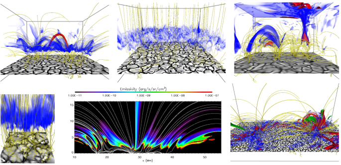

  

  3D (2D) view of the 3D (2D) publicly available numerical models. The 3D images show the emission of Si iv, Fe xii, and Fe xxi in blue, red, and green iso-surfaces, respectively. The plots correspond to simulations en024048_hion, ch024031_by200bz005, qs024048_by3363, qs006005_dyc, en096014_gol, and HGCR from left to right and top to bottom, respectively. The vertical velocity at the photosphere is shown in gray and the magnetic-field lines in yellow. For the 2D en096014_gol simulation (bottom middle) the map shows the emission in Si iv and the magnetic-field lines in white.

• iv) Simulation qs006005_dyc (Martínez-Sykora et al., 2019) mimics a coronal hole in which the corona has relatively low temperatures ($3\times 10^{5}~\text{K}$) and 2.5 G unsigned magnetic field. Because of the high resolution of this model, it is possible to investigate at small scales the kinetic–magnetic energy conversion (and local dynamo) in the upper-convection zone, photosphere, and chromosphere in the internetwork regions. Hydrogen ionization is in LTE and ambipolar diffusion is not included.

• v) Simulation en096014_nongol (Martínez-Sykora et al., 2018) is in 2.5D and mimics a plage region with two main polarities 40 Mm apart, connected with $\ge 40~\text{Mm}$ long loops. Hydrogen ionization is in LTE and ambipolar diffusion is not included. There is only a single snapshot, which is mostly used as a comparison to the next model. The 2.5 dimensions limit the braiding and types of waves present.

• vi) Simulation en096014_gol (Martínez-Sykora et al., 2018) has the same setup as en096014_nongol, but includes ambipolar diffusion and the Hall term. This model reproduces many aspects of Type-II spicules despite its obvious limitations: it is 2.5D, and ionization is treated in LTE. It also shows an interesting thermal evolution of low-lying loops.

• vii) The HGCR model (Cheung et al., 2019) is the first self-consistent 3D radiative MHD model (purl.stanford.edu/dv883vb9686) of a flare (equivalent to a GOES M class) driven by an emerging eruption. The setup is inspired by National Oceanic and Atmospheric Administration (NOAA) Active Region 12017, which appeared in late March and early April 2014. Contrary to the previous models, this one is computed with MURaM which assumes LTE and gray radiative transfer. Figure 4 shows the hot ribbons in Fe xxi (green).

4 Study of Fundamental Physical Processes in the Solar Atmosphere

In this section we review how IRIS observations and numerical modeling have contributed to a better understanding of several key fundamental physical processes that occur not only in the solar atmosphere but play a role throughout the heliosphere and astrophysical environments.

4.1 Chromospheric Heating and Ion–Neutral Interactions

The solar chromosphere is sandwiched between the relatively cool surface, or photosphere, and its million-degree outer atmosphere, or corona. While the chromosphere’s temperature is only modestly increased over that of the photosphere, the many scale heights of dense plasma comprising the chromosphere imply that up to two orders of magnitude more non-thermal energy are required to sustain the chromosphere as compared to the corona. Nevertheless, its dominant heating mechanisms remain unknown and determining which physical processes dominate the heating of the chromosphere is a major challenge in solar physics.

To tackle this long-standing problem, several different approaches are useful. It is important to properly diagnose thermodynamic conditions in the chromosphere and to develop theoretical models for various heating mechanisms, including numerical simulations. Detailed comparisons between observations and numerical models play an important role in studying the various mechanisms that contribute to heating the chromosphere. Here we focus on IRIS-related results; for a broader review, see Carlsson, De Pontieu, and Hansteen (2019).

4.1.1 Observations

Diagnosing chromospheric conditions is complex because many of the diagnostics are optically thick and formed under conditions that depart from local thermodynamic equilibrium (non-LTE). As discussed in Section 2.1, the development of the STiC inversion code allows much improved diagnostics of the thermodynamics in the chromosphere using the Mg ii h and k lines, which are very sensitive to chromospheric conditions. The combination of the STiC inversion code and machine-learning techniques has provided the community with the $\text{IRIS}^{2}$ database (Sainz Dalda et al., 2019). Exploitation in the near future of the $\text{IRIS}^{2}$ database (Figure 2) for a wide variety of solar targets and phenomena has the potential to drastically expand the quantitative constraints on numerical models, a key step for discriminating between various potential chromospheric-heating mechanisms.

An example of the inversion approach is the work by Gošić et al. (2018) who used STiC inversions to estimate the impact on chromospheric thermodynamics from the release of magnetic energy through cancelation of the pervasive weak magnetic fields in the internetwork. They found that while the local heating is significant, it likely does not play a dominant role in the average energy balance of the quiet-Sun internetwork chromosphere. The spatio–temporal filling factor of such cancelations, at the sensitivity of the current (i.e. pre-DKIST) state-of-the-art magnetic-field measurements, is not high enough. Recent coordinated SST and IRIS observations also highlight the possibility of significant heating from the interaction between pre-existing magnetic fields and recently emerged granular-scale internetwork fields (Gošić, De Pontieu, and Bellot Rubio, 2021). Such heating would be compatible with statistical studies (Schmit and De Pontieu, 2016) that suggest a heating component in the internetwork that is unrelated to the magnetic network or the ubiquitous magneto-acoustic shocks (which are presumed to dominate the local energy balance). To settle this issue, future coordinated DKIST/IRIS observations are needed, given the sensitivity of the IRIS diagnostics to the upper chromosphere and transition region.

The availability of chromospheric diagnostics from the IRIS Mg ii lines is particularly useful when combined with ground-based observations, which often have spectral lines or diagnostics that are highly complementary. For example, the combination of IRIS Mg ii h and k spectra and ALMA mm observations has been used (Figure 5) to discriminate more accurately between chromospheric temperature and non-thermal motions (da Silva Santos, de la Cruz Rodríguez, and Leenaarts, 2018; da Silva Santos et al., 2020). Similar synergies exist with other spectral lines formed in the chromosphere (Carlsson, De Pontieu, and Hansteen, 2019). New advances in the inversion techniques that are focused on incorporating measurements from different observatories with a wide range of spatial resolutions (de la Cruz Rodríguez, 2019) allow the community to fully exploit combined IRIS, ALMA, or DKIST observations.

Figure 5

Simultaneous inversions of IRIS and ALMA data provide unprecedented diagnostics of the chromospheric thermodynamic conditions, in this example temperature maps [kK] as a function of optical depth in a plage region. Such inversions show particular promise to help resolve the degeneracy between temperature and microturbulence (da Silva Santos et al., 2020).

Observational studies of heating in the magnetically dominated chromosphere have focused on a wide range of physical mechanisms. For example, magneto-acoustic shocks are ubiquitous not only in the internetwork but also in the magnetic network, plage, sunspots and penumbrae. They have a strong impact on the appearance of spectral lines wherever the shocks occur. However, it is not clear whether they are responsible for the bulk of the heating in the chromosphere. IRIS observations have been used to study their propagation and the evolution of non-linear harmonics as they travel upwards (Chae et al., 2018), as well as their frequency-dependent damping in sunspot umbrae (Krishna Prasad et al., 2017). Shock waves have also been studied (using coordinated data from DST or Hinode) in sunspot light bridges, with their provenance tied to magnetic reconnection and leakage of photospheric waves (Tian et al., 2018a; Bai et al., 2019). Similar processes have been invoked to explain the presence of high-frequency signals discovered in active-region plage (Narang et al., 2019). To determine whether these phenomena play a significant role in the local energy balance, novel techniques such as the $\text{IRIS}^{2}$ database and new methods to accurately determine shock-wave properties (Ruan et al., 2018), in combination with coordinated observations, will be very useful. Statistical approaches can also help elucidate the nature of the heating mechanism. For example, statistical analysis of the correlation between the photospheric magnetic field (from SDO/HMI) and IRIS diagnostics shows an intriguing decrease in correlation around the temperature minimum, followed by an unexplained increase towards the upper chromosphere (Barczynski et al., 2018), a challenge for future models.

Another approach to studying chromospheric heating is based on exploiting the correlations between physical variables (such as temperature, velocity, density) and synthetic observables (Rathore and Carlsson, 2015; Rathore et al., 2015; Leenaarts et al., 2016; Lin, Carlsson, and Leenaarts, 2017) derived from numerical simulations, primarily with the Bifrost code (Gudiksen et al., 2011). These types of correlations have been used to diagnose heating under a wide variety of conditions, from quiescent heating in the plage or quiet chromosphere (e.g. Pereira et al., 2015; Park et al., 2016) to the violent conditions in reconnection-driven Ellerman bombs (e.g. Vissers et al., 2015) and flares (e.g. Tian et al., 2015), thereby providing constraints on the physical mechanisms (e.g. reconnection, Alfvén waves, non-thermal electrons) responsible for the observed heating and dynamics. As more advanced numerical simulations become available for a wider range of solar targets (with the bulk of the results so far based on enhanced network simulations), the applicability of this approach will be enhanced.

Several of these techniques have been applied to the study of heating in plage, regions with strong magnetic field outside of sunspots. Simplified forward-models of Mg ii k emission combined with non-thermal broadening derived from O i (Carlsson, Leenaarts, and De Pontieu, 2015) suggest that plage regions show a step-like increase of heating in the low chromosphere and a transition region at high column mass, with significant non-thermal motions. More sophisticated inversions using STiC allow the height-dependent determination of these properties in plage, as shown by de la Cruz Rodríguez, Leenaarts, and Asensio Ramos (2016) using IRIS and SST observations. STiC inversions of combined IRIS Mg ii h/k spectra and ALMA mm radiation (Figure 5) above plage provide even more stringent constraints on how the temperature and turbulent motions depend on height (da Silva Santos, de la Cruz Rodríguez, and Leenaarts, 2018; da Silva Santos et al., 2020). Such inversions have also provided the first direct measurements of plage heating associated with magneto-acoustic shocks (see also Chintzoglou et al., 2021a,b). The excellent synergies between IRIS and ALMA observations also highlight a possible path to further improvements of the inversion approach from IRIS data alone: preliminary studies indicate that the C ii 1335 Å intensities are well correlated with ALMA band-6 intensities (which are a good proxy for temperature in the upper chromosphere), suggesting that $\text{IRIS}^{2}$ inversions that include C ii would enhance the fidelity of the temperature in the upper chromosphere, a region where the Mg ii h and k lines are less sensitive (Jafarzadeh et al., 2019; da Silva Santos et al., 2020).

4.1.2 Numerical Modeling

One of the key approaches of the IRIS investigation has been the comparison between synthetic observables from advanced numerical simulations and IRIS observations. In the Bifrost simulations, the bulk of the magnetic atmosphere is heated by dissipation of currents generated through magnetic-field line braiding (e.g. Hansteen et al., 2015). These numerical models of the chromosphere are highly complex because of the wide range of physical processes that may play a role in this dynamic region. Because of the computational cost, it is currently not possible to include into a numerical model all of the candidate physical processes suspected of playing a role in the chromosphere. The IRIS modeling approach has been to gradually include more diverse magnetic-field conditions (the main free parameter in the Bifrost models), as well as more complex processes, both guided by comparisons with the observations. A key driver for this approach has been the finding that synthetic observations of Mg ii h and k lines from Bifrost models are typically too narrow and often too faint compared to the high-resolution IRIS spectra (Carlsson, De Pontieu, and Hansteen, 2019). Various studies have been performed to understand this discrepancy. The lack of broadening in synthetic spectra could, in principle, be caused by a lack of turbulent motions in the numerical models. However, microturbulence can be estimated from the optically thin O i 1356 Å line in the IRIS FUV bandpass (Carlsson, Leenaarts, and De Pontieu, 2015) and is found to be insufficient to fully explain the discrepancy. This result suggests that in the Bifrost models there is a lack of opacity in the Mg ii lines, which could be caused by a lack of heating, mass loading, or density at chromospheric heights. One possibility is that the turbulent motions that are observed with IRIS are directly associated with a heating process that is missing from the models, such as heating from turbulence driven by the Farley–Buhnemann instability (Madsen et al., 2014) or Alfvén waves (Brady and Arber, 2016). Observational studies of the correlation between O i broadening and chromospheric heating using $\text{IRIS}^{2}$ inversions would be interesting to help settle this issue.

While it may not be easy to include physical mechanisms that occur on microscopic plasma scales into the Bifrost or other MHD models, it should be more straightforward to investigate the role of several other possible effects. For example, it is possible that numerical simulations at higher spatial resolution may lead to locally higher dissipation rates and subsequent heating, or even the generation of higher-frequency Alfvén or other waves (e.g. through vortical motions, Moll, Cameron, and Schüssler, 2011), both of which could contribute to more heating at chromospheric heights. Similarly, the interaction of small-scale, granular-scale fields with pre-existing network or plage fields is a possible candidate for explaining some of the heating in the magnetic chromosphere, also given the observational suggestions that cancelation of magnetic flux may play a role in heating the atmosphere (Chitta, Peter, and Solanki, 2018). Numerical simulations with more realistic magnetic-field distributions that attempt to capture the properties of granular-scale fields are important to investigate this issue. Recent simulations also suggest that small-scale magnetic fields may also be generated at chromospheric heights (Martínez-Sykora et al., 2019).

4.1.3 Ion–Neutral Interactions

An important aspect of the chromosphere is that it is partially ionized, like the Earth’s ionosphere. This can lead to dissipation of magnetic energy from interactions and slippage between the electrically charged ions and neutral particles. These effects have long been suspected of playing a significant role in the momentum and energy balance of the chromosphere. IRIS related numerical simulations have produced significant advances in our understanding of the role of ion–neutral interactions: ambipolar diffusion can lead to heating and significantly affect the dynamics of the chromosphere (Martínez-Sykora et al., 2015, 2016a, 2017a). In particular, these studies have provided new insights into our understanding of the formation and evolution of chromospheric spicules, the most common jets in the solar atmosphere (Martínez-Sykora et al., 2017a). Advanced numerical simulations show that ambipolar diffusion fundamentally changes the interaction between the strong network or plage magnetic fields and the ubiquitous granular scale weak fields. It allows these tangled weak fields to diffuse into the middle and upper chromosphere where the violent release of magnetic tension (introduced in the subsurface convection zone) leads to rapid acceleration of plasma to drive supersonic jets with speeds of $50\,\text{--}\,100~\text{km}\,\text{s}^{-1}$ that are heated while they expand upwards through the diffusion of ambipolar currents. Synthetic observables from these simulations show good agreement with IRIS and SST observations of spicules, including the significant heating to TR temperatures observed with IRIS and Hinode/SOT (Skogsrud et al., 2015; De Pontieu, Martínez-Sykora, and Chintzoglou, 2017). Modeling and observational results also suggest a significant impact of spicules on the corona (De Pontieu et al., 2017; Martínez-Sykora et al., 2018). During the past few years it has become clear that other mechanisms may also produce jet-like features, including magneto-acoustic shocks (e.g. Hansteen et al., 2006; Matsumoto and Shibata, 2010), vorticity, and twisted magnetic fields (e.g. Iijima and Yokoyama, 2017). It remains unclear which of these is the dominant formation mechanism in the solar atmosphere. To settle this issue will require several advances on the modeling side: the identification of these jets as spicules is often based on physical variables in the model rather than synthetic observables. Also, many of these models lack a more sophisticated treatment for the significant radiative losses in the chromosphere. Finally, observations of spicules now extend into the transition region, so a full comparison across all wavelengths is key. In the Bifrost models at least, the introduction of ambipolar diffusion appears to have a significant effect on the strength, ubiquity, and thermal evolution of spicule-like features in the models (see Figure 6).

Figure 6

Temperature and velocity parallel to the magnetic field in two models, one in which ion–neutral effects are neglected (panels A, C) and one that implements these effects using a generalized Ohm’s law (panels B, D). In the latter we find much longer fast spicules, similar to those observed, as a consequence of the increased role of ion–neutral effects such as ambipolar diffusion (adapted from Martínez-Sykora et al., 2017a).

Ion–neutral interactions can also produce damping of Alfvénic waves, especially at high frequencies (e.g. De Pontieu, Martens, and Hudson, 2001; Ballester et al., 2020), further enhanced by interaction between different species (e.g. Zaqarashvili, Khodachenko, and Rucker, 2011; Popescu Braileanu et al., 2019; Martínez-Sykora et al., 2020c). Detailed comparisons between numerical models and high-resolution observations with IRIS and DKIST of spicules, which are known to carry Alfvénic waves (De Pontieu et al., 2007a; Okamoto and De Pontieu, 2011; De Pontieu et al., 2014c), could provide evidence of ion–neutral damping of Alfvén waves and possible associated heating.

Recent simulations also highlight the importance of non-equilibrium ionization in the chromosphere, which is of importance for both hydrogen and helium (see, e.g., Golding, Carlsson, and Leenaarts, 2014). The combination of ambipolar diffusion and non-equilibrium ionization appears to lead to enhanced electron densities in the chromosphere. This causes increased opacity at least in the ALMA bands, with the effect on Mg ii opacity not yet known. Comparisons with IRIS–ALMA observations (Martínez-Sykora et al., 2020c) suggest that the increased ALMA opacity may explain puzzling observations of chromospheric “holes”: regions of unusually low temperatures ($<4000~\text{K}$) recently discovered with ALMA (Loukitcheva, White, and Solanki, 2019). These may occur as a result of low temperatures in the wake of magneto-acoustic shocks that provide mass to canopy loops. In addition, these simulations show that low-lying transition-region loops could be heated by ambipolar dissipation of electrical currents (Martínez-Sykora et al., 2020a).

Further developments of the numerical models (and comparison with observations) thus hold promise to address many unresolved issues, such as the role of the Farley–Buhnemann instability, thermal instabilities (Oppenheim et al., 2020), backwarming from Lyman-$\alpha$, vorticity and Alfvén waves, interactions between small-scale weak fields and strong network or plage fields, and the interactions between multiple fluids and species (e.g. Martínez-Sykora et al., 2020b).

4.2 Alfvén Waves

The strongly inhomogeneous solar atmosphere is a rich environment for wave processes. Magneto-convection, density stratification, and magnetic-field emergence lead to large complexity in the physics of wave propagation. Because of the pervasive character of MHD waves and their substantial energy content, understanding this complexity is necessary for understanding the solar atmosphere, including coronal heating and solar-wind acceleration.

Among MHD waves, Alfvén waves and, more generally, transverse MHD waves (defined here as having magnetic pressure and/or tension as one of the main restoring forces) are the ones to consider, due to their unique ability to carry enough energy to generate a corona (Uchida and Kaburaki, 1974; Cranmer and van Ballegooijen, 2005).

The study of transverse MHD wave generation and dissipation in the solar atmosphere is a field that has been significantly advanced by IRIS. Indeed, a high-resolution imaging spectrometer has a unique advantage to capture the 3D-flow associated with a wave, thereby more accurately identifying the nature of the wave. Furthermore, the temperature coverage of IRIS allows one to track the propagation of the wave across the chromosphere and transition region, where many wave processes are expected to occur.

For coronal-heating purposes, any wave generated in the lower atmosphere needs to first propagate through the chromosphere and transition region before reaching the corona. This interface region presents sharp density and magnetic-field gradients that lead to a significant loss of wave energy through processes such as mode conversion, shock heating, refraction, and reflection (Bogdan et al., 2003), as well as ion–neutral interactions. In-situ generation of transverse MHD waves by-passes these obstacles and is therefore an interesting path to explore. Coordinated IRIS–SOT coronal-rain observations have provided a new mechanism of in-situ transverse MHD wave generation in the corona through colliding flows, leading to energy fluxes of $10^{7}\,\text{--}\,10^{8}~\text{erg}\,\text{cm}^{-2}\,\text{s}^{-1}$. Similarly, theory predicts that a large fraction of the energy released through magnetic reconnection is in the form of Alfvén waves. IRIS has now observed this process, with the first fully resolved torsional Alfvén wave in the corona (Kohutova, Verwichte, and Froment, 2020, see Figure 7).

Figure 7

The first direct detection of a torsional Alfvén wave with slit-jaw image (SJI) 1400 observations (top row) and Si iv 1394 Åand Mg ii 2796 Å spectra (bottom panels). Top panels show three different phases of the torsional oscillation (each consisting of superimposed images at the times shown); the white dotted lines outline the helical trajectories (arrow shows direction of rotation). White vertical line indicate the IRIS slit crossing the motion. The spectral profiles covered by this slit portion are shown at three different times in the bottom panels. Vertical dashed lines indicate the mean Doppler velocity. The tilted dashed line indicates the torsional motion. Adapted from Kohutova, Verwichte, and Froment (2020).

The main wave generator in the solar atmosphere is magneto-convection and related processes such as magnetic buffeting (Kato et al., 2016), from which ample power is observed (e.g. Oba, Iida, and Shimizu, 2020). Horizontal displacement of magnetic bright points is expected to be an efficient generator of transverse MHD waves (e.g. Jafarzadeh et al., 2017). Recent statistical analysis of transverse waves on spicules using IRIS Mg ii spectra constrain the transverse wave amplitudes to $25~\text{km}\,\text{s}^{-1}$ (Tei et al., 2020), indicating significant wave-energy fluxes at those heights on the order of $0.1\,\text{--}\,3\times 10^{6}~\text{erg}\,\text{cm}^{-2}\,\text{s}^{-1}$. A 3 – 6% transmission into the corona leads to $1\,\text{--}\,2\times10^{5}~\text{erg}\,\text{cm}^{-2}\,\text{s}^{-1}$, which is sufficient for the quiet-Sun corona and acceleration of the solar wind, in line with previous measurements from Hinode/SOT (De Pontieu et al., 2007a).

Recently, vortical motions in the form of swirls in the photosphere have been ubiquitously detected (e.g. Liu et al., 2019). These structures are particularly interesting since they are expected to naturally generate torsional Alfvén and fast kink MHD waves, referred to as “Alfvénic” waves due to the magnetic-tension force being the main restoring force (Bonet et al., 2008; Wedemeyer-Böhm et al., 2012). An important question is whether such vortical structures carry through to the upper atmosphere and whether they represent any major energy and mass conduit for the corona. First simultaneous observations of a vortex at photospheric and chromospheric levels have been obtained through coordinated SST–IRIS observations (Park et al., 2016), indicating high-speed upflows and a potentially important role in the chromosphere–corona mass and energy cycle. This has further been supported by the detection of propagating Alfvén pulses from swirls with a factor of 10 – 80 times the required energy power for locally heating the chromosphere (Liu, Nelson, and Erdélyi, 2019). Chromospheric signatures of Alfvén waves from swirls have further been observed in case studies (Tziotziou, Tsiropoula, and Kontogiannis, 2020), while coordinated SST–IRIS observations have established the ubiquity of torsional motions on sub-arcsecond scales, occurring in active regions, quiet Sun, and coronal holes alike (De Pontieu et al., 2014b). These observations show how these waves propagate upward and are associated with heating to transition-region temperatures, as seen in IRIS Si iv 1402 Å images and spectra.

Perhaps the most important, but also most elusive, wave process in the solar atmosphere is mode conversion, which involves the change from a specific wave mode into another, and therefore a change in the 3D flow of the wave, as well as its compressive properties and thus its ability to dissipate. Several types of mode conversion are expected to occur, such as longitudinal to transverse mode at the Alfvén–acoustic equipartition layer in the chromosphere (Schunker and Cally, 2006) and fast mode to Alfvén mode in the transition region where a strong gradient in the Alfvén speed is expected (Cally and Hansen, 2011). These processes are yet to be directly observed, but work such as Kanoh, Shimizu, and Imada (2016) combining IRIS and SOT clearly shows the enormous change in wave-energy flux (from $10^{7}$ to $\approx10^{5}~\text{erg}\,\text{cm}^{-2}\,\text{s}^{-1}$) in the longitudinal modes during propagation from the photosphere to transition-region heights, suggesting either mode conversion or dissipation. If the former, such observations suggest a possible explanation for the ubiquity of Alfvénic waves in the corona (McIntosh et al., 2011), part of which show frequencies characteristic of $p$-modes (Morton, Weberg, and McLaughlin, 2019). If the latter, they provide evidence of an important chromospheric-heating contribution, as also supported by other work (De Pontieu et al., 2007b; Okamoto and De Pontieu, 2011; Morton et al., 2012; Liu, Nelson, and Erdélyi, 2019).

Besides the above linear mode-conversion processes, non-linear mode conversion is also expected and can involve Alfvén to slow/fast modes or longitudinal to transverse modes. It is driven by terms such as the ponderomotive force, flux tube expansion, or wave-to-wave interaction. A characteristic signature of this process is a doubling of the wave frequency and therefore the generation of high-frequency waves (Shoda and Yokoyama, 2018), which are commonly detected in spicules (e.g. Okamoto and De Pontieu, 2011; Srivastava et al., 2017; Tavabi and Koutchmy, 2019).

Mode conversion is also expected to occur ubiquitously in the corona because of its strongly inhomogeneous structure. Analogous to the fast to Alfvén mode conversion in the transition region, kink waves are expected to efficiently transfer their energy to azimuthal Alfvén waves (resembling the torsional $m=1$ Alfvén wave, Goossens et al., 2020), wherever the kink speed matches the Alfvén speed and in particular at the boundaries of coronal loops. Known as resonant absorption (or mode coupling), this process has long been hypothesized to be the leading explanation behind the observed strong damping of large-amplitude kink oscillations (Nakariakov and Kolotkov, 2020) and, together with the line-of-sight (LOS) superposition effect, is thought to be the main reason for the apparently small wave-energy flux in the corona. Indeed, this idea has received support from numerical simulations, showing that 10% or less of the wave energy is recovered from the plane of the sky (POS) motions detected with imaging instrumentation alone (De Moortel and Nakariakov, 2012; Antolin et al., 2016). On the other hand, a large fraction of the wave energy is expected to hide behind the observed large spectral-line broadening resulting from these processes (Pant et al., 2019), naturally explaining the observed correlation between Doppler velocities and line widths (McIntosh and De Pontieu, 2012). However, this interpretation of non-thermal motions as evidence for waves has recently been brought into question by IRIS results. Li and Peter (2019) captured the injection of plasma into a loop, associated with the injection of helicity, strong helical motions, and (possibly) the subsequent development of turbulence (from line broadening). While such broadening is typically interpreted in terms of waves, the observed scenario may also be compatible with recent braiding models. To settle this interesting issue, more observations and advanced models are required. Coordinated IRIS and Solar Orbiter/Spectral Imaging of the Coronal Environment (SPICE) measurements of line broadening in the same structure but from different vantage points will help distinguish between various mechanisms (Section 4.5).

Despite the overwhelming theoretical support for resonant absorption, direct observational evidence was only possible through IRIS–SOT coordinated observations of a prominence. An out-of-phase relation between the POS oscillatory motion (detected with SOT) and the LOS velocity (detected with IRIS) and accompanying heating of the prominence threads from $10^{4}~\text{K}$ to, at least, $10^{5}~\text{K}$ was observed (Okamoto et al., 2015). Through numerical simulations, such signatures were shown to be telltale signatures of resonant absorption (Antolin et al., 2015a, see Figure 8). Furthermore, the Kelvin–Helmholtz instability (KHI) produced by the velocity shear from the transverse displacement and the resonance was shown to play a major role, allowing the enlargement of the resonant layer (to the observable scale) and the establishment of turbulence leading to wave dissipation and heating. This work has opened a very active research avenue for wave-based coronal heating. Further coordinated observations and modeling are required to determine how common this phenomenon is in other, more prevalent, structures in the solar atmosphere.

Figure 8

Coordinated IRIS and Hinode/SOT observations of an active prominence at the limb, reported by Okamoto et al. (2015). Heating signatures were captured, seen by fading of the prominence threads in the SOT Ca ii H line (yellow) accompanied by intensity increase in the hotter SJI 1400 passband (gray). The Doppler velocity captured by IRIS in the Mg ii k line (purple dots in bottom-left time–distance panel) shows an out-of-phase motion with respect to the plane-of-the-sky motion captured by SOT. 3D MHD simulations of an oscillating prominence thread with a kink mode performed by Antolin et al. (2015a) reproduce the heating signatures and phase relations, based on the combined effect from resonant absorption and the KHI, as shown in the sketch. Figure taken from Van Doorsselaere et al. (2020).

The Transverse Wave-Induced Kelvin–Helmholtz (TWIKH) rolls predicted by the KHI-resonant-absorption model have received further support in coordinated SST–SOT observations of spicules (Antolin et al., 2018). A very good match was found between the model and the observed characteristic strand-like structure in intensity (Skogsrud, Rouppe van der Voort, and De Pontieu, 2014) and Doppler velocity, the very fast apparent upward motion (De Pontieu, Martínez-Sykora, and Chintzoglou, 2017) and ragged Doppler-shift sign changes at maximum transverse displacement. On the other hand, the model has so far only been found to lead to mild temperature increase, at odds with IRIS observations combined with SDO and SST showing the TR to coronal heating impact of spicules (De Pontieu et al., 2014a; Skogsrud et al., 2015; Skogsrud, Rouppe van der Voort, and De Pontieu, 2016; De Pontieu et al., 2017). More advanced simulations suggest that the observed heating and Alfvénic waves (and thus potentially the TWIKH rolls as well) may be a consequence of a whiplash effect from the release of magnetic tension through ambipolar diffusion (Martínez-Sykora et al., 2017a).

Several heating models based on Alfvénic waves have been proposed (Van Doorsselaere et al., 2020). Besides the combined KHI-resonant absorption model (e.g. Karampelas et al., 2019), the long established Alfvén-wave turbulence model (based on wave-to-wave interaction, e.g. van Ballegooijen et al., 2011; Matsumoto, 2018) and, more recently, the generalized phase mixing model (Magyar, Van Doorsselaere, and Goossens, 2017), all rely on the establishment of turbulence for wave dissipation to occur. It remains unclear whether the observable signatures from these models and, in particular, the observed non-thermal line broadening at both chromospheric and coronal levels match observational constraints. Measurements of non-thermal broadening of the optically thin O i line at the chromospheric footpoints of coronal loops (Carlsson, Leenaarts, and De Pontieu, 2015) place strict constraints on the available wave-energy flux. At the coronal level, constraints come from measurements of Alfvén waves in coronal rain (Kohutova and Verwichte, 2016). Coronal rain investigation can further strongly constrain the wave-energy flux in the corona since it uniquely combines the possibility of high-resolution observations of coronal plasma (catastrophically cooling and thus becoming observable in the IRIS temperature range, Antolin, 2020), with a strong reduction of the LOS superposition effect (due to the increased optical thickness). Combined observations of prominences and coronal rain between Solar Orbiter/Extreme Ultraviolet Imager-High Resolution Imagers (HRI) and IRIS may not only provide the phase relations between velocity, line width, and intensity characteristic of resonant absorption and KHI processes, but may also directly observe the turbulent heating events that result. Furthermore, the high resolution provided by DKIST may also allow to distinguish the nature of the turbulence by directly observing TWIKH rolls. For example, the double mode-conversion process, through which $p$-modes may convert into Alfvénic waves in the transition region and corona, may be detectable through coordinated IRIS–DKIST observations.

4.3 Shock Waves

Oscillatory signals are common in the chromosphere. In many locations these lead to the formation of shocks as they propagate upward from the photosphere into the rarified chromosphere. Shock waves have long been known to pervade the chromosphere, from the quietest internetwork regions to stronger magnetic-field regions such as network, plage, and sunspots. There have been extensive numerical-modeling efforts aimed at understanding the role of shock waves for several decades (Carlsson and Stein, 1997; Bogdan et al., 2003), both in weak and stronger magnetic-field environments. Studying shock waves with IRIS has given insight into how such waves behave in a complex magnetic environment where they often cross the plasma-$\beta =1$ surface(s), and also how they impact the energy balance of the chromosphere, transition region or corona.

IRIS observations of shock waves in internetwork regions show that these waves only rarely impact the transition-region emission (Martínez-Sykora et al., 2015). This is quite different in stronger field regions as seen in IRIS observations of sunspots (Tian et al., 2014b; Yurchyshyn, Abramenko, and Kilcik, 2015), which reveal the impact of shocks on the transition region above sunspots. Coordinated Hinode/SP and IRIS observations of sunspots have allowed determination of photospheric and upper chromospheric energy fluxes carried by slow-mode magneto-acoustic shock waves, revealing that these shocks play an important role in heating the sunspot chromosphere (Kanoh, Shimizu, and Imada, 2016). Furthermore, recent IRIS observations and numerical modeling have now uncovered the existence of pseudo-shocks (i.e. exhibiting only density discontinuity) in C ii spectra above sunspot umbrae, carrying a large energy flux upward (Srivastava et al., 2018a). The pseudo-shock represents a discontinuity in density akin to the entropy mode (cf. Section 4.9.2). It is still unclear what the drivers of pseudo-shocks are and how ubiquitous they are.

By applying the helioseismic time–distance analysis technique on measurements with IRIS, SDO/HMI, SDO/AIA, and the 1.6 m Goode Solar Telescope at the Big Bear Solar Observatory (BBSO), Zhao et al. (2016) have traced the source of some shock waves all the way to below the solar surface. Leakage of photospheric waves is also seen in sunspot light bridges, although reconnection in the lower atmosphere also appears to play a role in generating waves in light bridges (Tian et al., 2018a). This is further discussed in Section 4.7.

Magneto-acoustic shocks also play a significant role in the dynamics and heating of the upper chromosphere and low transition region above plage, as shown by analysis of coordinated SST and IRIS observations (Skogsrud, Rouppe van der Voort, and De Pontieu, 2016) where they are seen to drive dynamic fibrils (Hansteen et al., 2006) and strong brightenings in transition-region lines (Figure 9). In fact, many of the rapidly evolving brightenings in IRIS slit-jaw images are caused by slow-mode magneto-acoustic shocks.

Figure 9

Slow-mode magneto-acoustic shocks are ubiquitous in active-region plage, dominating the temoral evolution, as shown by sawtooth patterns in $\lambda$–time plots in chromospheric lines (middle and right panels) and the resulting formation of jets called dynamic fibrils. The impact of these jets on the transition region leads to a multitude of short-lived brightenings at the transition-region footpoints of coronal loops (Si iv, left panel) (Skogsrud, Rouppe van der Voort, and De Pontieu, 2016). ©AAS. Reproduced with permission.

In strong-field regions such as network and plage, IRIS observations suggest a link between these chromospheric shocks and the long-elusive propagating coronal disturbances (Bryans et al., 2016; De Pontieu et al., 2017) that continuously occur along coronal loops and that have been attributed to slow-mode waves or flows that supply mass and/or energy to the corona. Other coordinated IRIS–AIA observations have tied the shocks in umbrae to propagating intensity disturbances in the corona, suggesting they may play a role in the coronal energy balance (Hou et al., 2018). This is further discussed in Section 4.9.

IRIS observations have also shown that chromospheric shocks are not only driven from below, as previously thought, but also occur when strong coronal or TR downflows slam into the chromosphere. This has been observed both in sunspots, e.g. Straus, Fleck, and Andretta (2015), and arch-filament systems created by flux emergence (see Toriumi, Katsukawa, and Cheung, 2017, who use Hinode/SOT, SDO, and IRIS data).

Given the ubuiquity of magneto-acoustic shocks, quantifying their contribution to the momentum and energy balance of the chromosphere is important. To determine whether shocks (or any other phenomenon) are energetically significant, typically the energy flux is estimated and compared to the average radiative losses expected from the chromosphere. The latter are most often based on spatio–temporal averages from semi-empirical models (e.g. Withbroe and Noyes, 1977). This approach could be improved upon significantly if instead of averaged radiative losses the locally determined radiative losses are used (Díaz Baso, de la Cruz Rodríguez, and Leenaarts, 2021). In future work, this could be achieved by exploiting high-fidelity inversions either through STiC or $\text{IRIS}^{2}$ to determine the local thermodynamic conditions in the atmosphere and calculating the associated radiative losses.

4.4 Fundamental MHD Instabilities

The solar atmosphere allows for the investigation of fundamental MHD instabilities in extreme conditions unattainable in the laboratory. Such instabilities can play a key role in major solar questions, such as the dissipation of MHD waves or the onset and rate of magnetic reconnection, but they can also provide seismological insight into the local conditions in which they form. With its high resolution and large temperature coverage, IRIS has provided key new insight into these processes.

The Kelvin–Helmholtz instability (KHI) is an MHD shear-flow instability characterized by vortex-shaped, self-similar structures at the interface of velocity-shear regions. Importantly, in the high magnetic Reynolds number of the solar atmosphere, small-scale structures are generated in the turbulent cascade that results, allowing the kinetic and magnetic energy of the flow to be dissipated into heat, as well as momentum transfer due to the strong mixing of the plasma components across the shear boundary (Fujimoto and Terasawa, 1994). The KHI can also induce more efficient radiative cooling by enlarging the population of transition-region plasmas in chromospheric–coronal interface regions (Hillier et al., 2019; Fielding et al., 2020), whose temperatures can be detected with IRIS.

In magnetized plasmas, magnetic tension can inhibit the KHI onset, and therefore shear flows misaligned to the magnetic field will more readily trigger the instability since the magnetic-tension component opposing the unstable modes is effectively reduced (Chandrasekhar, 1961). Periodic transverse-shear flows, as in the boundary of coronal loops oscillating with kink modes, are always KHI unstable (or unstable to a similar parametric instability, Hillier et al., 2019), and a large number of numerical studies supports such findings (e.g. Terradas et al., 2008; Antolin, Yokoyama, and Van Doorsselaere, 2014, see Section 4.2). However, observations of the KHI have been scarce so far, either limited to quiescent prominences (e.g. Berger et al., 2010, see also Section 4.9.3) or to very energetic events, such as CME eruptions (Foullon et al., 2011) or flares (Brannon, Longcope, and Qiu, 2015; Yuan et al., 2019). Observations of the KHI in quiescent prominences with IRIS suggest that only large field-aligned shear flows (with Alfvén Mach number larger than 2) are able to trigger the instability in such conditions (Hillier and Polito, 2018, see also Figure 18 and Section 4.9.3). On the other hand, 3D MHD simulations of eruptions have shown that the characteristic KHI vortices (and Alfvénic vortex shedding at the wake of the eruption) are only visible for very specific LOS and at high resolution, and they indicate that spectroscopic instruments are largely favored over imaging instruments to readily detect the characteristic features (Syntelis and Antolin, 2019). Accordingly, broadened line profiles accompanied by vortex motions have been observed by IRIS at the top of loop arcades with null-point topologies (Liu, Antolin, and Sun, 2016), resembling the quiescent prominence dynamics. In an observation that is the first of its kind, the formation of the KHI produced by a blowout jet has been captured by IRIS exhibiting shear-flow speeds of several $100~\text{km}\,\text{s}^{-1}$, a small-scale saw-tooth pattern at the shear flow boundary and a temperature increase of $\approx 2~\text{MK}$ during the event, indicating kinetic- and magnetic-energy dissipation (Li et al., 2018c).

Another fundamental MHD instability of magnetized plasmas observed in the solar atmosphere is the Rayleigh–Taylor instability (RTI). This instability forms at the interface of two fluids with large density variation, where magnetic tension works against gravity to support the denser fluid. In the solar atmosphere it has been observed in quiescent prominences, through the characteristic formation of tenuous but hotter plumes, which rise through the dense material. Because of the partial ionization state of the prominence material, an interesting effect predicted by numerical simulations is the formation of localized large velocity drifts between the neutral and ion populations, due to the difference in the instability dynamics for both populations (Khomenko et al., 2014; Popescu Braileanu et al., 2019). The existence of such velocity drifts carries large importance due to its effect on physical quantities such as wave damping and the magnetic-reconnection rate. While recent results provide support for such multi-fluid physics, more observations are needed to understand such plasma dynamics (Anan, Ichimoto, and Hillier, 2017; Wiehr, Stellmacher, and Bianda, 2019).

Recently, the first coupled KHI–RT instability has been observed with SOT in a quiescent prominence (Berger, Hillier, and Liu, 2017). Large shear-flow velocities of $100~\text{km}\,\text{s}^{-1}$ were inferred at the interface of prominence bubbles based on the observed phase velocity. However, reduced RT growth rates were measured, attributed to the existence of magnetic shear estimated to be on the order of 10 G at an angle of $70^{\circ }$ to the prominence plane in order to compensate the effect from the velocity shear flow. The existence of such large shear flows in prominence bubbles has been confirmed thanks to IRIS observations (Berger, Hillier, and Liu, 2018) and could lead to a better determination of the magnetic field in such bubbles, also in coordination with DKIST.

Thermal instability is yet another fundamental plasma instability whose understanding has been significantly advanced thanks to IRIS observations. Thermal instability is discussed in Section 4.9.2, together with its main observable feature (coronal rain).

Finally, MHD instabilities can also play a role in reconnection (e.g. during flares) and the large-scale destabilization of the solar atmosphere (e.g. the torus instability). This is discussed in Section 5.2 and Section 5.3.

4.5 Dynamics of Braiding

Braiding of magnetic fields, resulting from the interaction between the convective motions and magnetic fields, and subsequent reconnection and dissipation of magnetic energy has been proposed as a dominant coronal-heating mechanism – an alternative to Alfvén wave dissipation. The theory of braiding, or nano-flare heating, was first proposed by Levine and Altschuler (1974) but convincingly elaborated by Parker (1983, 1988) and later developed further by Cargill (1994). In summary, large-scale photospheric motions drive the magnetic field to form large gradients in the chromosphere and corona as field lines of varying angles are forced together. These gradients are formed at small scales, eventually causing episodic dissipation at the same small scales. The dissipation events are known as nano-flares as they were first predicted to have a magnitude some $10^{-9}$ of a typical flare. These ideas were tested in early numerical simulations (Galsgaard and Nordlund, 1996; Hendrix and van Hoven, 1996) which showed that indeed small-scale current sheets, the site of episodic dissipation, rapidly form as a result of the forcing of motions in a line-tied magnetic field. It is not clear how ubiquitous or dominant braiding is in the solar atmosphere, nor what the detailed properties of this mechanism are. However, several 3D numerical models, also in a realistic solar setting, show that braiding likely occurs as a result of coronal field lines being advected by photospheric flows (Gudiksen and Nordlund, 2005; Hansteen et al., 2015; Rempel, 2017). Braided field lines, even at small angles to each other are shown to lead to episodic nano-flare dissipation of sufficient strength to heat the outer solar atmosphere to coronal temperatures. Thus braiding appears to provide a possible viable answer to the coronal-heating problem. The unanswered questions concern the mode of dissipation (as current numerical models cannot reach kinetic-dissipation scales) and the importance of heating through braiding as compared to wave or other forms of heating (as these may not be captured well by existing models).

Several IRIS results during the past few years have found evidence that supports braiding as a significant contributor to the energy balance of the outer atmosphere. For example, coordinated IRIS, Hinode/XRT, and Hinode/EIS observations of moss, the upper transition-region footpoints of hot coronal loops, reveal evidence for small-scale heating events at transition-region heights. The sub-arcsecond spatio–temporal patterns and center-to-limb variations of flows and non-thermal motions in these events, as derived from the highest-resolution Fe xii measurements made, are compatible with numerical models of coronal heating from braiding and appear in conflict with predictions from Alfvén wave-heating models (Testa, De Pontieu, and Hansteen, 2016).

Similar signatures of small-scale reconnection are found in low-lying cooler active-region loops that only reach transition-region temperatures. These signatures are visible in sub-arcsecond resolution IRIS Si iv spectra as strong brightenings with anomalously broadened profiles and are associated with the formation of loops (Huang et al., 2015, 2017). Using IRIS and AIA observations, Bahauddin, Bradshaw, and Winebarger (2020) suggest that brightenings in Si iv and O iv are consistent with magnetic-reconnection-mediated impulsive heating at field-line braiding sites. The observations suggest that impulsive heating occurs as a consequence of magnetic reconnection in multi-stranded transition-region loops and that the line profiles indicate the possible importance of ion-cyclotron turbulence caused by strong currents at the reconnection sites. However, the large velocities (close to Alfvénic) found suggest that it is large-angle reconnection that may be occurring, rather than the smaller-angle “component” reconnection predicted by braiding theory and simulations. Further studies are needed to determine whether the heating is caused by reconnection as a result of flux emergence or as a result of braiding.

Pontin, Peter, and Chitta (2020) investigate why the non-thermal broadening in most transition-region and coronal lines is of the order of $15\,\text{--}\,30~\text{km}\,\text{s}^{-1}$, this seemingly independent of the instrument resolution (De Pontieu et al., 2015a), and further, why there is a correlation of line intensity and the non-thermal broadening (Testa, De Pontieu, and Hansteen, 2016), and why the line profiles are non-Gaussian with enhanced power in their wings. The authors construct a 3D numerical model of a coronal loop and suggest that line broadening with these characteristics is caused by the turbulent decay of an initially braided magnetic field, and thus is evidence that braiding is a strong actor in heating the outer solar atmosphere. They do find that the line broadening is more pronounced perpendicular to the magnetic field than parallel to it, but claim that this finding may not hold up under coronal conditions where the perpendicular component of the field is expected to fall off more slowly than the parallel component with height. In either case, simultaneous observations of similar spectral lines with IRIS and Solar Orbiter/SPICE from different vantage points would provide unique constraints on such models. Future studies of the properties of line broadening in various magnetic-field topologies, and in active regions of varying ages, plage, and quiet Sun at different locations on the solar disk, and comparisons of these with the synthetic observables derived from numerical models will clarify this issue further and constrain the importance of the braiding mechanism.

Low-lying transition-region loops are likely related to the so-called “unresolved fine structure” (UFS) loops (see Figure 10) whose existence had been predicted from Skylab observations and which were discovered to be ubiquitous in IRIS slit-jaw images of quiet-Sun regions (Hansteen et al., 2014b). Statistical studies of their properties and comparisons with hydrodynamic simulations have now revealed that these loops indeed appear to be resolved by IRIS (Brooks, Reep, and Warren, 2016). The loops show collective behavior on cross-field spatial scales that are of order 300 km, wich is much larger than the spatial scales predicted from theoretical models of magnetic-energy dissipation in the solar atmosphere. Brooks, Reep, and Warren (2016) suggest that this spatial scale could be caused by the switch-on nature of the “secondary instability” – one of the proposed physical mechanisms involved in the dissipation of currents driven by braiding. Pereira et al. (2015) suggest that flux emergence may play a role in forming some of these loops, although it remains unclear to what extent this is the case. As a result, it is not clear whether such low-lying loops are a good proxy for how coronal loops are heated or whether their low-lying nature implies a larger role for flux emergence than for typical loops in the solar atmosphere. Statistical studies of the properties of these loops and their relationship to the magnetic field could help address this open question.

Figure 10

IRIS Si iv slit-jaw images reveal highly dynamic, low-lying loops at transition-region temperatures (adapted from Hansteen et al., 2014a). (A) UFS-loops on the western solar limb. (B) the same field of view is shown, but with SDO/AIA images: the coronal 171 Å (blue) and 193 Å (green) filters, note that the UFS-loops are hidden by the high opacity of cool gas at these wavelengths. The loops are rapidly evolving as shown in three regions of interest in the small panels. Such loops are presumably heated episodically by braiding induced or flux-emergence-induced reconnection. In active regions, low-lying loops are also common, connecting nearby plage regions of opposite polarity (Huang et al., 2015). These types of loops provide a unique sub-arcsecond resolution view of features that may have similar heating mechanism(s) to (some) coronal loops.

Recently, exciting IRIS results have revealed direct observational signatures of fast ($>100~\text{km}\,\text{s}^{-1}$), short-lived ($\approx15~\text{seconds}$), and small-scale ($<1^{\prime \prime }$) jet-like features (Figure 11), typically perpendicular to a cool loop-like structure, and associated with nano-flare-sized heating events (Antolin et al., 2021). Initially, the loop shows misaligned rain strands and complex rotational motions, compatible with the existence of braiding in the loop. The nanojets precede the formation of coronal strands, leading to a hot coronal loop. Comparison with numerical models suggest that these are reconnection events predicted from braiding, with spatio–temporal properties characteristic of an MHD avalanche. This is supported by the expansion of the nanojets across and along the loop, their increase in frequency of occurrence and the overall reduction in the misalignment of the rain strands over time. These nanojets represent a key signature of magnetic reconnection leading to coronal heating. It is not yet clear whether these features are related to the jet-like threads and visible braiding seen with IRIS in erupting loops (Huang et al., 2018) and to other similar small-scale jet-like structures seen in tornadoes with IRIS (Chen et al., 2017, 2020). On the other hand, visible braiding or twisting at sub-arcsecond scales in non-erupting low-lying loops is not detected in observations that exploit the high-resolution of IRIS and of the High-resolution Coronal imager (Hi-C) 2.1 ($<0.5^{\prime \prime }$; Rachmeler et al., 2019), suggesting that field relaxation may prevent build-up of highly braided structures with many twists, consistent with early numerical work on braiding (Galsgaard and Nordlund, 1996) and compatible with recent MHD braiding models.

Figure 11

Examples of nanojets – a smoking gun of reconnection-based coronal heating – as observed by IRIS (adapted from Antolin et al., 2021; their Figure 2a, Figure 4d, and Figure 6). Top-left panels: Time series of IRIS 1400 SJI images showing a cluster of nanojets. Top-right panels: Example of IRIS Si iv (bottom) spectra of the nanojets. Bottom row: Sketch of the reconnection process leading to a nanojet: Loop-like structures observed in the POS undergo a slow upward expansion (brown arrows); the stars denote the nano-flares, for which the evolution is shown in the other panels. Small misalignments between the green and magenta field lines lead to reconnection at small angles, and plasma is heated and advected transversely to the loop at large speeds due to magnetic tension, thereby creating the nanojet. The inward component is much larger than the outward component (red arrows) due to the curved topology of the field lines, thus leading to the singular nature of the jet. A final configuration is reached with reduced braiding and misalignment between field lines at a higher temperature. A coronal strand starts to form.

Coordinated IRIS–Solar Orbiter/Extreme Ultraviolet Imager (EUI) observations are required to settle the issue of whether field relaxation is effective in hindering the build up of strongly twisted field or whether most braiding causes reconnection at small angles. Despite the many observational clues for braiding in the low solar atmosphere, more extensive statistical studies are needed and expected to provide key insight into the role and mode of braiding in the solar atmosphere.

4.6 Non-thermal Particle Acceleration and Chromospheric Response to Coronal Nano-Flares

Diagnosing physical processes in the corona, such as reconnection or particle acceleration, can be extremely difficult because of the optically thin nature of the corona and the long line-of-sight integration. The transition region and chromosphere form boundaries to the corona and do not suffer as much from these drawbacks. They can therefore be used to diagnose coronal-heating properties by observing the impact of small heating events (nano-flares) on the lower atmosphere.

Recent IRIS observations have demonstrated the potential for probing the properties of coronal nano-flares even while only observing the chromospheric and transition-region response to such small-scale heating events (Testa et al., 2014; Testa, Polito, and De Pontieu, 2020). Coordinated IRIS and AIA observations detected small-scale brightenings on timescales of $\approx10\,\text{--}\,30~\text{seconds}$ in chromospheric and transition-region emission, at the footpoints of the hottest ($\approx5~\text{MK}$) coronal loops in an active region (as observed with AIA). The AIA and Hinode coronal observations of these transient hot loops suggest that they are likely caused by relatively large-angle ($\gtrsim 20^{\circ }$) reconnection (Reale et al., 2019; Testa and Reale, 2020), yielding short-lived ($<60~\text{seconds}$) heating events leading to chromospheric and TR response. Such rapid brightenings were previously seen with the Hi-C coronal-imaging rocket experiment, but the exact physical mechanism remained elusive (Testa et al., 2013). The addition of IRIS spectra showed Si iv blue-shifted emission for several of these brightenings (Testa et al., 2014). Comparisons with advanced radiation-hydrodynamic modeling with RADYN showed that such upflows are not compatible with energy release at coronal heights followed by thermalization and thermal conduction to the footpoints (Testa et al., 2014; Polito et al., 2018a). Instead the observations are naturally explained by the generation of non-thermal electrons in the corona, which are thermalized when the beams reach the chromosphere. The wide thermal coverage of IRIS and AIA combined with the IRIS spectra appear to provide strict constraints for the properties of the electron beams, especially the low-energy cutoff.

Hard X-ray observations are directly observing emission from non-thermal particles and are generally considered the measurement of choice for investigating accelerated particles. However, these new diagnostics with IRIS are of particular interest for several reasons: First, they observe smaller (nano-flare-sized) events compared to hard X-ray observations, which typically detect micro-flares and larger flares (e.g. Christe et al., 2008; Hannah et al., 2011). New observations of small events with NuSTAR are possible (e.g. Glesener et al., 2020), but they are still few and challenging, and they yield non-thermal electrons (NTE) properties in agreement with the IRIS diagnostics of Testa et al. (2014) and Testa, Polito, and De Pontieu (2020). In addition, the IRIS observations more easily constrain the important low-energy cutoff parameter, which is difficult to derive from hard X-ray observations because of the typical dominance of the thermal emission at lower energies.

A follow-up statistical study to Testa et al. (2014), including ten different datasets and a large grid of numerical models exploring a broad region of the parameter space, pointed to an additional diagnostic of the presence of non-thermal particles, namely emission in the Mg ii triplet (around $\approx2798.8$ Å) observed by IRIS, as well as to more stringent constraints on the NTE-distributions (Figure 12) derived by using both chromospheric and TR diagnostics (Testa, Polito, and De Pontieu, 2020). This study reveals that NTE appear to be present in a significant fraction (≈ half) of the studied small heating events, including the smallest ones. These findings not only provide constraints on particle-acceleration mechanisms, but also highlight the presence of nano-flare-sized heating events in the corona and show that non-thermal particles play a role in heating at least the hottest coronal loops in AR cores. These results also show that IRIS chromospheric and TR observations offer the opportunity to investigate the physics of electron beams with higher sensitivity, i.e. for smaller events than often possible with hard X-ray observations from instruments such as RHESSI and NuSTAR (e.g. Testa et al., 2014; Hannah et al., 2016; Wright et al., 2017). Significant additional progress in the study of NTE outside large flares can be made with future investigations for instance by carrying out larger statistical studies of such heating events, and by combining IRIS with additional chromospheric and/or hard X-ray coordinated observations to further pin down the properties of NTE and heating distributions.

Figure 12

IRIS observations of rapid variability ($\lesssim60~\text{seconds}$) at the footpoints of transient hot coronal loops in active-region cores (adapted from Testa, Polito, and De Pontieu, 2020) provide spectral diagnostics of the properties of coronal heating and energy transport (thermal conduction or non-thermal electrons, NTEs). Left panels (a): IRIS 1400 SJI and AIA 94 Å images (top panels) showing the footpoint brightenings and the hot ($\approx8\,\text{--}\,10~\text{MK}$) coronal emission, respectively; temporal evolution of intensity in various IRIS spectral lines (middle-left), and of the spectral properties of Si iv and Mg ii (bottom-left); time series of IRIS spectral observations during the brightenings (bottom-right). Right panels (b): Histograms of observed IRIS properties of footpoint brightenings (from top): Si iv Doppler velocity, Si iv non-thermal line broadening, duration of the moss brightening in Si iv, and ratio of intensity maxima for C ii/Si iv and Mg ii/Si iv. The colored symbols show the corresponding predictions of different RADYN models including heating exclusively by thermal conduction (C1), by a combination of thermal conduction and NTE (H1, H2), or by NTE only (E1 – E6, with increasing energy [5, 10, 15 keV] from orange to green to blue; see Testa, Polito, and De Pontieu, 2020 for details). ©AAS. Reproduced with permission.

Non-thermal electrons also appear to leave their mark in small-scale jets. Innes et al. (2015) find evidence for apparently super-Alfvénic “jets” in IRIS slitjaw images that protrude from small-scale reconnection events. They suggest a scenario in which reconnection events (observed as Si iv explosive events) generate electron beams that propagate away from the source at speeds of thousands of $\text{km}\,\text{s}^{-1}$, while the weak interaction with the background loop plasma leads to thermalization of a fraction of the electrons, thereby forming linear brightenings in the IRIS slitjaw images. These intriguing results clearly require more modeling and analysis. Furthermore, IRIS TR lines emitted by transition-region ions in active regions often show evidence of significant wing emission, departing from a single Gaussian shape, and they can be well fitted with non-Maxwellian $\kappa$-distributions (Dudík et al., 2017). These non-Maxwellian distributions exhibit significant power-law tails at high velocities or energies, and can be caused by a variety of processes, including acceleration of particles due to magnetic reconnection, shocks, wave–particle interactions, or plasma turbulence. Their study, and modeling, can provide crucial information on the physical processes at work during flares and active-region heating events. Numerical modeling of such events also highlights the diagnostic potential of IRIS to detect effects of non-equilibrium ionization (Bradshaw and Testa, 2019), or departures from Maxwellian distribution (Dzifčáková and Dudík, 2018), which are key to a proper interpretation of IRIS data.

4.7 Magnetic Reconnection in Small-Scale Events

Reconnection of magnetic-field lines is thought to drive a variety of energetic events, e.g. flares or CMEs, but also much smaller events further down in the atmosphere. Reconnection occurring during flares is discussed in Section 5.2. Here we focus on reconnection in smaller events occurring in the lower solar atmosphere. UV bursts, sudden and compact brightenings in UV emission, provide an opportunity to study magnetic reconnection on the Sun (Young et al., 2018). A variety of phenomena such as transition-region explosive events and IRIS bombs are considered to be UV bursts. These events provide an opportunity for studying fundamental aspects of reconnection and its impact on the solar atmosphere.

4.7.1 UV Bursts

Recent IRIS results have capitalized on the discovery of IRIS bombs, or now more commonly called “UV bursts” (Peter et al., 2014). UV bursts are short-lived Si iv events driven by convergence and cancelation of opposite polarity flux (Tian et al., 2018b; Wu, 2019), in which plasma is accelerated to $>100~\text{km}\,\text{s}^{-1}$ and heated to what appear to be TR temperatures at low chromospheric heights. These “bombs” or “bursts” are related to phenomena named “explosive events” as reported by earlier instruments such as High Resolution Telescope and Spectrograph (HRTS: Dere, Bartoe, and Brueckner, 1989) or SOHO/Solar Ultraviolet Measurements of Emitted Radiation (SUMER: Innes et al., 1997). Statistical studies using IRIS and ground-based telescopes (e.g. SST and GST), show that some (but not all) UV-bursts appear to be closely related to the well-known Ellerman bombs (e.g. Vissers et al., 2015; Kim et al., 2015; Tian et al., 2016a; Grubecka et al., 2016; Ortiz et al., 2020) while at the same time some 20% of observed Ellerman bombs have associated UV-bursts. Coordinated IRIS and ground-based observations show that the IRIS bombs are associated with reconnection between granular scale oppositely directed field in the photosphere (Gupta and Tripathi, 2015; Kim et al., 2015), e.g. triggered by flux emergence (Toriumi, Katsukawa, and Cheung, 2017); similar conditions to those found in Ellerman bombs.

An analysis of a variety of spectral diagnostics shows that the hot UV-burst plasma is emitted at very high densities (as demonstrated by self-absorption in Si iv lines, see Yan et al., 2015) typical for upper-photospheric or low-chromospheric conditions. It is also clear that the temperatures are at least an order of magnitude higher than 1D non-LTE models for Ellerman bombs can produce (Grubecka et al., 2016). This argument is further strengthened by the existence in the Si iv 1402 Å line of a very narrow Ni ii absorption feature (as well as other lines of Fe ii typically associated with photospheric temperatures).

Because of the rich diagnostic capabilities of IRIS from the photosphere to the transition region, UV-bursts provide the most detailed views of reconnection events in the solar atmosphere. Coordinated IRIS and SST observations show how the overlying canopy of chromospheric fibrils hides the reconnection site from view in commonly used ground-based diagnostics like the $\text{H}\alpha$ core, while IRIS observables such as C ii (upper chromosphere), Si iv(transition region), and Mg ii triplet (low chromosphere) lines see through this absorbing forest and unveil the “bomb” site (Vissers et al., 2015). Along with the derived temperatures and densities described above, these direct views revealed puzzling and hotly debated results about the formation heights and the temperatures to which plasma is heated in UV bursts. Initially, some argued that the Si iv emission with superimposed cool absorption lines (Gupta and Tripathi, 2015) is caused by heating to 80,000 K (Peter et al., 2014) at photospheric heights. This was strongly contested by Judge (e.g. 2015) based on radiative transfer considerations, or with alternative suggestions of, e.g., 10 – 20,000 K based on LTE ionization (Rutten, 2016).

There is now consensus, based on observational evidence and numerical modeling (see Figure 13), that the Ellerman bomb and UV burst, when they occur together, are formed at the opposite ends of the extended current sheet resulting from the interaction of recently emerged field with itself or with the pre-existing ambient field. The absorption seen in Ni ii and Fe ii is caused by cool gas carried high into the chromosphere, above the strongly emitting current sheet, as emerging flux breaks free of the photosphere and expands upwards into the corona (Hansteen et al., 2019). Coordinated IRIS and GBO observations have confirmed how Ellerman bombs and UV bursts (Figure 13), when they occur together, appear to be formed at different heights (Chen et al., 2019a), although still being part of the same reconnection system (Ortiz et al., 2020).

Figure 13

Simultaneous observations in the red wing of the $\text{H}\alpha$ line made at the Goode Solar Telescope and in IRIS Si iv slit-jaw images near the solar limb show a displacement (upper-left panels) that is consistent with Ellerman Bombs and UV bursts forming at different heights along the same current sheet (upper-right panel, adapted from Chen et al., 2019a). This scenario is consistent with numerical models of flux emergence in which several magnetic “bubbles” pierce the photosphere and reconnect along nearly the vertical current sheets formed by their expansion and interaction (lower panels, adapted from Hansteen et al., 2019). ©AAS. Reproduced with permission.

A statistical study of the properties of UV bursts (using IRIS spectra and SDO/HMI magnetograms), their formation environments, and the impact on the chromosphere would provide a robust set of observational constraints for multi-fluid models of reconnection in the partially ionized plasma of the solar chromosphere. Such data will also provide insight into the geometry and topology of current sheets in areas of newly emerging magnetic flux – a topic of great interest since this flux eventually fills and pervades the solar corona. A better understanding of this process can be sought by confronting numerical modeling (e.g. Hansteen et al., 2019) with IRIS observations, supplemented (when available) with DKIST, SST, SDO, Solar Orbiter, or Hinode data.

Coordinated IRIS and GBO data will also be useful to study the intriguing reports of Ellerman-bomb-like features in QS (Nelson et al., 2017). Using the SST, Joshi, Rouppe van der Voort, and de la Cruz Rodríguez (2020) found evidence for ubiquitous, but weaker, Ellerman-bomb-like events in the $\text{H}\beta$ line with potential implications for the heating of the quiet Sun chromosphere, and Rouppe van der Voort et al. (2021) find similar events in sunspot penumbrae. This should be followed up with IRIS studies of chromospheric and transition-region observables.

4.7.2 Magnetic Reconnection Mechanisms in the Low Solar Atmosphere

IRIS observations have led to new results that have improved our understanding of how magnetic reconnection occurs in the solar atmosphere. For example, UV bursts and transition-region explosive events have provided insight into the detailed mechanisms involved in facilitating fast reconnection. It has long been known that reconnection in the solar atmosphere, which leads to dynamic events that occur on timescales of seconds or minutes, appears to proceed at a much faster rate than classical reconnection (e.g. Sweet–Parker, see Priest, 2014) theories predict for solar conditions.

Recent developments in reconnection theory suggest that under certain conditions slow reconnection can transition to fast reconnection when mediated by the plasmoid (or tearing-mode) instability. Evidence for reconnection mediated by plasmoids has now been found by comparing recent numerical models with IRIS observations of telltale “triangular-shaped” spectral line profiles in transition-region explosive events (Innes et al., 2015). Such profiles do not match predictions from the alternative fast (Petschek-type) reconnection. The presence of small-scale plasmoids has been directly confirmed through analysis of coordinated IRIS–SST observations of small-scale reconnection events in the low solar atmosphere and comparison with numerical models (Rouppe van der Voort et al., 2017). Evidence for this mechanism has also been found with IRIS in coronal jets (Zhang and Ni, 2019), flux cancelation events (using IRIS and AIA, Yang et al., 2018a), as well as much larger flares to explain propagating sawtooth-like and quasi-periodic flare-ribbon structures (Brannon, Longcope, and Qiu, 2015; Parker and Longcope, 2017). The reconnection-driven nanojets reported in the corona also exhibit plasmoid ejecta along their axis, particularly for the most energetic nanojet clusters (Antolin et al., 2021). More indirect but similar constraints come from IRIS observations of microflares, which provide support for fractal-type reconnection mediated by the secondary tearing instability (Reep et al., 2016a).

A very recent interesting finding is the discovery of a transition between slow and fast reconnection in very-high-cadence IRIS spectra. Comparison with numerical models shows that the observations are compatible with a transition from classical reconnection to fast reconnection mediated by plasmoids (Guo et al., 2020, Figure 14). On the other hand, some recent studies suggest that another mechanism (turbulence) appears to drive fast reconnection in some microflares (Chitta and Lazarian, 2020). More observations and modeling are required to determine how common both of these mechanisms are and their relative importance. Such observational insights can come from IRIS observations of the Ellerman bomb/UV burst phenomenon, which can provide important clues on the process of magnetic reconnection and the formation and evolution of the AR magnetic field. Unlike SDO/AIA passbands and GBO $\text{H}\alpha$ observations, the IRIS spectral bands are not opaque to the fibrils that overlie most bursts, allowing clear views of the reconnection process.

Figure 14

High-cadence observations of UV bursts or transition-region explosive events have revealed a rapid transition from bi-directional flows to complex, often triangular-shaped profiles (panels c, d), which agree well with numerical simulations of the transition from slow Sweet–Parker-like reconnection to fast reconnection mediated by the plasmoid instability (panels a, b) (Guo et al., 2020). ©AAS. Reproduced with permission.

Novel insights into the conditions that lead to reconnection have been obtained from so-called “light walls” (also called peacock tails) that originate not only from sunspot light bridges (Bharti, 2015), but also around neutral lines in and around, sunspots, as evidenced by a statistical study of six months of IRIS data (Hou et al., 2016a). Numerical simulations and IRIS and SDO observations have revealed the peculiar magnetic-field configuration in light bridges that leads to reconnection (Toriumi, Katsukawa, and Cheung, 2015; Toriumi, Cheung, and Katsukawa, 2015). IRIS observations have also elucidated the cross-field coherence in dynamic evolution of these lightwalls, which has been associated with slipping reconnection (Hou et al., 2016b; Bai et al., 2019): the light-wall dynamics appear to be intimately tied to, and thus help reveal the overall changes in, magnetic topology during a flare. High-resolution spatial and temporal data from IRIS and SDO have been used to confirm the observation of signatures of magnetic reconnection and accompanying flux cancelation (Yang et al., 2018b) including two-loop interaction processes, plasma blob ejections, and sheet-like structures above the flux-cancelation sites. Further studies of the conditions that lead to reconnection using the rich IRIS data archive are key to go beyond case studies and establish how common these mechanisms are. Coordinated IRIS and Solar Orbiter/EUI observations of so-called campfires (small-scale and short-lived heating events in the EUV) can help identify the role of reconnection in driving these recently discovered events (Berghmans et al., 2021).

4.8 Effects of Flux Emergence on the Chromosphere and Beyond

As magnetic fields rise from the photosphere into the low atmosphere, they interac driving dynamic events (Section 4.7) and energizing plasma (e.g. Cheung and Isobe, 2014). Recent IRIS results have shed light on the details and importance of this process. Emergence of magnetic field into the atmosphere occurs on many spatial scales, from active-region-size emergence down to small flux elements that continuously emerge on granular scales. In sum, the flux-emergence process on all scales fills and replenishes the chromospheric and coronal field, countering the depletion caused by reconnection, losses through the solar-wind, and submergence. Both the local and global topology of the emerging field play important roles in determining the heating rate in the outer atmosphere and the mode of solar wind acceleration. Furthermore, understanding flux emergence will enable a deeper insight into the processes active in driving the solar dynamo. Coordinated IRIS, SDO/HMI, and Hinode/SOT observations have led to new insights into the impact of this new flux on the energetics of the atmosphere in a variety of regions. For example, the early stages of AR flux emergence can be tracked very well through the development of UV bursts (Tian et al., 2018b), providing insight into how newly emerged flux interacts with pre-existing fields. Such insights have also come from coordinated IRIS–AIA observations showing counterparts of low-atmospheric UV-bursts in all coronal AIA passbands (Guglielmino, Young, and Zuccarello, 2019), suggesting long-lasting reconnection episodes between emerging and ambient fields. During the later phases of emergence, UV bursts may be less common, with energization higher up in the atmosphere when new loops interact with ambient coronal loops (Huang et al., 2019b).

Coordinated IRIS and SST observations of small-scale flux emergence in active regions reveal the general mechanism through which coronal magnetic fields are added into a new active region (Ortiz et al., 2016). These large-scale fields are built up through successive emergence of small-scale fields on granular scales. Each emergence of granular scale fields leads to cool bubbles that slowly rise into the atmosphere, which leads, after many minutes, to reconnection and upper-chromospheric and TR heating if the incoming fields are not well-aligned with the pre-existing fields.

For example, flux emergence plays a key role in the formation of the serpentine magnetic fields that drive reconnection events that lead to strong acceleration and low atmospheric heating that is visible as Ellerman or IRIS bombs (see Section 4.7.1 for more details and Figure 15 for an example). Toriumi, Katsukawa, and Cheung (2017) show that flux emergence can also lead to strong TR downflows along the arch-filament systems formed as a result of emergence. These supersonic downflows lead to shocks when they hit the chromosphere, leading to significant heating (visible in the Mg ii triplet lines).

Figure 15

IRIS 1330 SJI and spectra of the C ii, Si iv, O iv, and Mg ii h and k lines in an active region in its earliest emerging phase (adapted from Tian et al., 2018b). Strong heating and plasma acceleration, i.e. UV bursts, occur at sites where the emerging field interacts with itself or the pre-existing ambient coronal field. ©AAS. Reproduced with permission.

Weak magnetic fields continuously emerge in the quiet-Sun internetwork, and are considered a potential contributor to the heating of the QS chromosphere. Gošić et al. (2018) used IRIS and SST observations and found that cancelations of such elements are unlikely to play a significant role in bulk chromospheric heating at the sensitivity levels of high-cadence SST measurements, although coordination with deeper magnetograms from SST or DKIST are required to definitively settle this issue. On the other hand, the flux emerging in small magnetic loops may play an important role. Coordinated, high-resolution, multiwavelength observations obtained with the SST and IRIS of internetwork magnetic loops as they emerge into the photosphere reaching the chromosphere and transition region have recently been studied by Gošić, De Pontieu, and Bellot Rubio (2021). In this case study, the footpoints of the emerging internetwork bipoles are clearly seen to appear in the photosphere and to rise up through the solar atmosphere. Polarimetric measurements taken in the chromospheric Ca ii 8542 Å line provide direct observational evidence that internetwork fields are capable of reaching the chromosphere. The concurrent IRIS data show the effects of these weak fields on the local heating of the chromosphere and transition region. This work dovetails neatly with the discovery of $\text{H}\beta$ “Ellerman bombs” (Joshi, Rouppe van der Voort, and de la Cruz Rodríguez, 2020). Future coordinated IRIS and SOT, SST, or DKIST observations are needed still to determine whether emergence into the chromosphere plays an important role at a global level, i.e. whether the spatio–temporal filling factor of these events is large enough to impact the average energy balance of the internetwork chromosphere.

Flux emergence of course also plays a major role in driving flares and CMEs, the main exponents of space weather, as described in Section 5.3.

4.9 Energy and Mass Transfer Between Photosphere, Chromosphere and Corona

All coronal plasma has its origins in the lower solar atmosphere, with the coronal-mass budget driven by a balance between upward mass transport through, e.g., evaporative or eruptive flows, and the downward mass transport through, e.g., coronal rain or gentle cooling downflows. Although ultimately the coronal mass escapes into the heliosphere as the solar wind and to a lesser extent ($\approx1\%$) as CMEs or coronal jets, a fraction of coronal plasma returns to the chromosphere through downflows, forming a chromosphere–corona mass cycle (Marsch et al., 2008; Berger et al., 2011; McIntosh and De Pontieu, 2012). Many processes appear to be involved and the outstanding challenge is to determine which processes dominate in the various solar regions (quiet Sun, coronal hole, active region, sunspots).

4.9.1 Solar Jets and Surges

The solar atmosphere exhibits a wide variety of ejective phenomena, ranging from coronal jets, at the largest scales, down to penumbral microjets, at sub-arcsecond scales. Observed in virtually all electromagnetic ranges, these ejective phenomena are of broad interest because of their implication in the energy and mass balance of the chromosphere, transition region, and corona.

The major improvements in observational and computational capabilities over the past decades have yielded new insight into the still open questions related to formation of solar ejections. A representative example is spicules: the most ubiquitous jets in the solar atmosphere. Since their discovery, a huge effort has been performed to understand the generation mechanisms of spicules and their role to heat the solar corona (see, e.g., Beckers, 1968; Hollweg, Jackson, and Galloway, 1982; Sterling, 2000; De Pontieu, Erdélyi, and James, 2004; Hansteen et al., 2006; Rouppe van der Voort et al., 2009; Pereira, De Pontieu, and Carlsson, 2012). Concerning the role of IRIS in this progress, Pereira et al. (2014) exploited the broad thermal coverage provided by coordinated IRIS and Hinode observations (see Figure 16) to determine why spicules often fade rapidly from chromospheric passbands. They found that a significant fraction of chromospheric spicules undergo strong heating to at least transition-region temperatures, a fact that was also found by Skogsrud et al. (2015) through IRIS and Hinode data and Rouppe van der Voort et al. (2015) with IRIS and SST measurements on the solar disk. These articles suggest a spicule model that consists of multiple threads with different heating. Some threads reach TR temperature while others remain at chromospheric temperatures. These observations also provide key constraints for theoretical models and considerable numerical effort has been carried out to unravel the spicule formation. For example, Martínez-Sykora et al. (2017a,b) concluded that heating of spicular plasma to TR temperatures can be reproduced by their model, where ambipolar diffusion is a key mechanism in both the formation and heating of spicules. Later, it was shown that, when including non-equilibrium effects of hydrogen and helium, spicules have larger temperature variations and that ambipolar diffusion primarily acts in shock fronts and hot regions within the spicules (Martínez-Sykora et al., 2020a). Furthermore, Antolin et al. (2018) used coordinated IRIS and SOT observations and identified various types of Alfvénic waves with specific phase relationships in time and space, as well as a multi-stranded structure. These observations were found to be compatible with numerical models of transverse wave-induced Kelvin–Helmholtz rolls (see also Section 4.2) along spicules. More sophisticated modeling that includes both the dynamic formation of spicules, ambipolar diffusion, and complex wave phenomena are key to further investigate the heating mechanism(s) in spicules.

Figure 16

Quiet-Sun spicule images extracted from Pereira et al. (2014). Top panel: two of the IRIS slit-jaw filtergrams, SOT Ca ii H filtergrams, and the AIA He ii 304 Å channel. Middle panel: color composite of observations, where the red channel corresponds to the IRIS Mg ii k filtergram and the green and blue channels (cyan color) to the SOT Ca ii H filtergram. Bottom panel: composite image using the IRIS Mg ii k and Si iv filtergrams, for the same instant as the middle panel and a larger field. The dotted rectangle denotes the field-of-view of the middle panel. ©AAS. Reproduced with permission.

Other avenues have been recently opened to further explore spicules. For instance, combining IRIS and radio observations obtained with ALMA, Yokoyama et al. (2018) and Shimojo et al. (2020) showed that ALMA spicular-like observations correspond well with the IRIS counterpart, which is key for the diagnostics and interpretation of ALMA data. Furthermore, theoretical support for such coordinated observations has been also provided by synthetic observables from numerical experiments, e.g. Martínez-Sykora et al. (2020c), Chintzoglou et al. (2021b). Another example is the use of machine-learning techniques, where Bose et al. (2019) applied k-means to SST Ca ii and $\text{H}\alpha$ data to characterize the chromospheric spectral profiles of on-disk spicules, thereby leading to their unambiguous identification in Mg ii k.

IRIS has also been crucial to study other phenomena linked to spicules such as propagating disturbances and network jets. For the former, IRIS and SDO/AIA observations indicate that spicules appear to be the root of some coronal propagating disturbances (Pant et al., 2015; Samanta, Pant, and Banerjee, 2015; Bryans et al., 2016); however, it remains unclear whether these propagating disturbances are caused only by waves or whether flows of heated material are also injected into the corona during such events. Concerning network jets, it has been argued that they are the TR counterpart of spicules (Tian et al., 2014d; Narang et al., 2016; Chen et al., 2019b; Qi et al., 2019) with fast apparent motions ($>100~\text{km}\,\text{s}^{-1}$); nonetheless the combination of models and observations (De Pontieu, Martínez-Sykora, and Chintzoglou, 2017; Chintzoglou et al., 2018) suggest that many of these jets may actually be rapidly propagating heating fronts along spicules, rather than caused by mass motions. Further modeling and observations are required to settle these issues, and thereby address the energy and mass flux associated with these events.

In addition to the step forward in the understanding of the spicules and related events, IRIS observations have revealed significant TR emission associated with phenomena that were traditionally related to the chromosphere such as surges (Yokoyama and Shibata, 1995; Canfield et al., 1996; Chae et al., 1999; Brooks, Kurokawa, and Berger, 2007; Guglielmino et al., 2010, among others). By means of flux-emergence experiments carried out with the Bifrost code, Nóbrega-Siverio, Moreno-Insertis, and Martínez-Sykora (2016) showed that there is a significant part of the surge plasma that can be efficiently heated up to TR and even coronal temperatures, and then rapidly cools back to chromospheric temperatures. This result implies that, during the ejection of surges, it is possible to detect TR emission. Evidence of such emission was independently found in the IRIS Si iv lines by Nóbrega-Siverio et al. (2017) and Guglielmino, Young, and Zuccarello (2019). Other examples of chromospheric ejections with associated TR emission observed with IRIS are fan-shaped jets originating from light bridges (Yang et al., 2015; Bharti, 2015; Bai et al., 2019) and penumbral microjets (Vissers, Rouppe van der Voort, and Carlsson, 2015; Humphries et al., 2020), although penumbral microjets are not genuine jets with significant mass motions, but rather manifestations of heat fronts (Esteban Pozuelo et al., 2019; Buehler et al., 2019; Rouppe van der Voort and Drews, 2019; Drews and Rouppe van der Voort, 2020). In order to properly understand the TR emission of the aforementioned phenomena, one has to take the highly dynamic nature of the chromosphere into account as well as the fact that some elements in the TR have long ionization and recombination timescales, leading to relevant non-equilibrium ionization effects (e.g. Olluri, Gudiksen, and Hansteen, 2013; Olluri et al., 2015; De Pontieu et al., 2015b; Martínez-Sykora et al., 2016b). For instance, in the particular case of surges, Nóbrega-Siverio, Moreno-Insertis, and Martínez-Sykora (2018) showed that the sheath of these ejections suffers heating and cooling processes in short timescales due to the efficient action of mechanisms such as Joule heating, thermal conduction, or optically thin losses, thus producing significant departures from the statistical ionization equilibrium in Si iv and O iv ions. The non-equilibrium ionization effects could moreover be a natural explanation for some of the puzzling correlations between TR intensity and non-thermal line broadening that had been discovered with Skylab in the 1970s.

Within the catalog of ejective phenomena, coronal jets have also received a noticeable development thanks to IRIS observations. For instance, Cheung et al. (2015) used IRIS and SDO data to study recurrent coronal jets, which until then had been difficult to explain. They assimilated SDO/HMI magnetograms into a data-driven simplified MHD model with the aim of comparing with IRIS images and spectra. Thus, they were able to quantify the helical nature of the jets and found that emergence of current-carrying magnetic field supplies sufficient magnetic twist to drive recurrent helical jets. Signatures of transfer of twist to jets were also explored more recently by Liu et al. (2018a) and Joshi et al. (2020b). IRIS has also been key to studying the multi-temperature components of coronal jets (Mulay, Del Zanna, and Mason, 2017; Guglielmino et al., 2018; Lu et al., 2019; Cai et al., 2019; Ruan et al., 2019); analyzing their fan–spine topology (Jiang, Zhang, and Yang, 2015); obtaining evidence of Kelvin–Helmholtz instabilities associated with blowout coronal jets (Li et al., 2018c); and analyzing the sub-arcsecond structure of multiple blobs, possibly produced by the tearing-mode instability, that are ejected together with coronal jets (Zhang and Ni, 2019). In addition, through IRIS and SDO observations, Joshi et al. (2020a) found that the characteristics of the observed surges and kernels (plasmoids) that accompany the coronal jets, as well as the detected double-chambered structures show striking similarities with numerical jet models (see, e.g., Moreno-Insertis and Galsgaard, 2013; Nóbrega-Siverio, Moreno-Insertis, and Martínez-Sykora, 2016).

4.9.2 Coronal Rain

Coronal rain is a phenomenon that was initially considered only as a specific kind of prominence (Levine and Withbroe, 1977), and it was not until the advent of high-resolution instrumentation and multi-temperature coverage of the transition from chromosphere to corona that its unique characteristics were recognized. IRIS played a fundamental role in this process, marking the unique links to multiple fundamental plasma processes.

Coronal rain corresponds to cool and dense, clumpy plasma appearing seemingly out of nowhere in the solar corona on a timescale of minutes, and falling back towards the solar surface along coronal loops (Antolin, 2020). It is a catastrophic cooling phenomenon from coronal to chromospheric temperatures and can thus, in a way, be considered as the opposite of coronal heating. This fascinating cooling problem, representing somewhat “snowflakes in the oven”, holds many unsolved mysteries upon which IRIS has shed new light.

The leading explanation for coronal rain is thermal instability in the solar atmosphere, which can occur when radiative losses locally overcome the heating gains. Due to the shape of the radiative-loss function with respect to temperature, runaway cooling occurs, which can lead to the growth of unstable thermal modes (also known as entropy modes) that produce a local loss of pressure and a subsequent accretion of material to form a condensation (Field, 1965; Müller, Peter, and Hansteen, 2004; Claes and Keppens, 2019).

The rapid recombination process on a timescale of minutes was first resolved through IRIS–SOT observations by Antolin et al. (2015b) by combining the SJI 1400, 1330, and 2796 passbands with the Ca ii H filter of SOT (Figure 17) (see also Liu et al., 2014b; Antolin et al., 2014). A fast–slow two-step cooling process was observed suggesting either the transition from optically thin to optically thick cooling, or the presence of a heating source linked to the compression produced by the rain on the downstream plasma. Strong changes in the morphology are observed along the magnetic-field direction (taken as the direction of the flow), with longer tails at the wake of the rain at transition-region temperatures, thereby potentially playing a role in the characteristic filamentary morphology of coronal loops observed in transition region to low coronal temperatures, as seen in AIA 171 Å. Prior to IRIS and SST observations, coronal rain was considered as a sporadic phenomenon of active regions, whereby catastrophic cooling would occur in a loop at most once every two days (Schrijver, 2001). Despite the large evidence for cool chromospheric and transition-region downflows from coronal heights (Levine and Withbroe, 1977; Kjeldseth-Moe and Brekke, 1998), and EUV downflow signatures (both bright from emission or dark from absorption, e.g. Ugarte-Urra, Winebarger, and Warren, 2006; O’Shea, Banerjee, and Doyle, 2007; Warren et al., 2007; Tripathi et al., 2009; Kamio et al., 2011) there was no direct link between the two, and thereby no consensus for the physical mechanism of such multi-thermal downflows.

Figure 17

(a) Coronal rain along an active-region loop at the limb observed with IRIS in the SJI 1400 (green) and SJI 1330 (blue), and with SOT in the Ca ii H line (red). (b) A zoomed-in view on the yellow rectangle shown in (a) of a coronal-rain clump observed with the various filters, ordered in ascending temperature formation order from left to right, Ca ii H (SOT), SJI 2796, SJI 1330, SJI 1400, and AIA 304. Each row corresponds to three time instances, with each column showing the snapshot closest in time to the SOT snapshot. Figure adapted from Antolin et al. (2015b). ©AAS. Reproduced with permission.

On the other hand, observations with SST have revealed that these warm flows contain a large number of small cool chromospheric cores with densities on the order of $10^{11}~\text{cm}^{-3}$ or higher (see Figure 17, Antolin et al., 2015b; Froment et al., 2020), suggesting a tip-of-the-iceberg clump distribution in which the bulk at smaller sizes may still be unresolved. Combined, these chromospheric and transition-region return flows to the solar surface show mass-flux values on the order of $1\,\text{--}\,5\times 10^{9}~\text{g}\,\text{s}^{-1}$ (similar to prominences), suggesting that most of the material in the loop undergoes catastrophic cooling. Therefore, it is now clear that coronal rain plays an important role in the chromospheric–corona mass and energy cycle.

In the direction perpendicular to the flow (the latter is expected to trace the magnetic field), the width of the interface from chromospheric to transition-region temperatures is observed to be very sharp, below $0.33^{\prime \prime }$, evidencing the highly structured and multi-temperature corona at unparalleled spatial resolution (Figure 17 and Antolin et al., 2015b). This fact also illustrates the highly anisotropic nature of thermal conduction in the solar corona. Another characteristic feature of coronal rain shown by these authors is its multi-stranded structure, particularly in the chromospheric lines, in the direction perpendicular to the field. Although still an open question, it has been argued that such morphology should naturally result from the spatial structure of the unstable thermal modes (van der Linden and Goossens, 1991).

The dynamics of such cool downflows further challenge our understanding of the solar atmosphere. Despite the high coronal origins, the falling speeds are on average on the order of $100~\text{km}\,\text{s}^{-1}$, with maxima close to $200~\text{km}\,\text{s}^{-1}$ (Schad et al., 2016; Schad, 2017). While the kinetic energy of these flows can be comparable to that of a microflare, and indeed lead to brightenings in the visible and UV spectrum upon impact (Kleint et al., 2014; Deng et al., 2016; Hou et al., 2016c; Ishikawa et al., 2020; Nelson, Krishna Prasad, and Mathioudakis, 2020), with termination shocks (Straus, Fleck, and Andretta, 2015; Chitta, Peter, and Young, 2016) and strong chromospheric oscillations (Kwak et al., 2016), the speeds of the downflows, and in particular the observed acceleration, are usually a factor of three lower than that expected from gravity, suggesting other forces at play (Antolin, Shibata, and Vissers, 2010; Antolin and Rouppe van der Voort, 2012). Oliver et al. (2014) have shown that the condensation process generates a restructuring of the gas pressure downstream of the rain. The acceleration process therefore occurs mainly in a timescale given by the sound speed, with heavier rain clumps experiencing stronger acceleration through a yet unidentified physical effect.

Some of these downflows are observed to be persistent over a puzzlingly long time, much longer than the draining time of a loop (Straus, Fleck, and Andretta, 2015; Chitta, Peter, and Young, 2016) and have thus favored a siphon-flow interpretation over that of coronal rain. 2D MHD simulations by Fang, Xia, and Keppens (2013) show, however, that coronal rain can have a siphon-like nature, with the siphon flows becoming thermally unstable along the way. The intermittent and clumpy nature of coronal rain is also observed to become more continuous and persistent just before impact due to a funnel effect from the expansion of the magnetic field with height (Antolin et al., 2015b). These effects combined can therefore provide an explanation to the plume-like and filamentary structure of coronal loops often observed above sunspots (Foukal et al., 1974).

The amount of thermally unstable material in the corona at any one time is still unclear. However, IRIS has made it clear that coronal rain is a far more common and pervasive phenomenon than previously thought. This is supported by recent results from Samanta, Tian, and Prasad Choudhary (2018). Using 60 large IRIS rasters above active regions, it was found that 80% of the datasets present high-speed downflows at chromospheric to transition-region temperatures.

Coronal rain is not only an active-region phenomenon. Indeed, new IRIS and AIA observations (in the 304 Å passband) indicate the common occurrence of this phenomenon in QS coronal loops associated with null-point topologies, where the presence of magnetic dips are common and help accumulate material that subsequently becomes thermally unstable (Liu et al., 2014a; Mason, Antiochos, and Viall, 2019; Li et al., 2018a, 2019a, 2020b). In this scenario, interchange reconnection between open and closed loops is invoked to explain the presence of coronal rain within the closed loops, although it is yet unclear if reconnection itself plays a direct role in the generation of coronal rain. This seems indeed possible, as suggested by IRIS observations from Kohutova, Verwichte, and Froment (2019).

The link between coronal rain and coronal heating has been highlighted by the discovery of long-period EUV intensity pulsations (Auchère et al., 2014; Froment et al., 2015). This phenomenon corresponds to highly periodic pulsations in most EUV passbands lasting up to a week in coronal structures in both active and quiet-Sun regions. Simulations have shown that the driver mechanism is very likely thermal non-equilibrium (Antiochos, DeVore, and Klimchuk, 1999; Froment et al., 2017, 2018). This scenario is presented by footpoint concentrated heating that is frequent enough (with a mean recurrent time less than the radiative cooling time), leading to cycles of heating and cooling (also known as evaporation and condensation cycles), with periodic EUV flows (Pelouze et al., 2020). Although globally the loop is in a non-equilibrium state, during the cooling stage thermal instability can set in to produce coronal rain (Antolin, 2020).

Observations of coronal rain further allow a direct high-resolution window on the coronal topology and dynamics, as shown by, e.g., Antolin and Verwichte (2011) and Nelson et al. (2019) for the detection of Alfvénic waves, and, e.g., Antolin et al. (2021) for the detection of braiding-induced reconnection.

The advent of new instruments on Solar Orbiter and DKIST provides exciting new opportunities to address unresolved issues regarding coronal rain. For example, Solar Orbiter/EUI will provide an effective spatial resolution in the EUV of 200 km or less, which, together with IRIS and DKIST/VBI observations in the chromospheric lines, will address whether the fine multi-stranded structure of coronal rain extrapolates to the entire coronal-loop structure. If so, this would establish thermal instability as one of the main causes behind the filamentary morphology of the corona and would more strongly constrain the energy transport scales.

Combined observations with IRIS and DKIST/VISP and DL-NIRSP will allow to observe the fast recombination process involved in catastrophic cooling leading to coronal rain. The details of this process – e.g. how cool coronal rain can get, how does the cooling rate change from the optically thin to thick regimes – may provide an insight into the plasma composition and processes beyond MHD such as ambipolar diffusion.

4.9.3 Prominence Diagnostics

Another manifestation of “snowflakes in the oven” on the Sun is prominences (Tandberg-Hanssen, 1995; Vial and Engvold, 2015), some mysteriously cool and dense material found at elevated heights in the hot and tenuous corona. Unlike coronal rain, which is usually small in size and transient in time, prominences are relatively large-scale, long-lived structures that generally appear as bright emission at the limb and dark absorption on the solar disk (thus called filaments). Prominences play important roles, not only in the mass budget of the corona with prominence drainage serving as the return flow of the chromosphere–corona mass cycle (together with coronal rain, e.g. Liu, Berger, and Low, 2014; Liu et al., 2018b), but also in solar activity with prominence eruptions forming the cores of CMEs (see Section 4.9.4 and Section 5.3). For example, about ten large quiescent prominences of typically $3\times 10^{16}~\text{g}$ each, e.g. Gopalswamy and Hanaoka (1998), can hold the mass equivalent to the entire solar corona. Consisting of numerous downflow streams at typical speeds of $\approx 10~\text{km}\,\text{s}^{-1}$, a single large prominence is capable of draining the entire corona in just about one day, at a rate twice that of the mass loss to the solar wind.

The mass supply to prominences is a key aspect of the chromosphere–corona mass cycle and the transfer of mass into the outer atmosphere in general, which has remained a topic of debate with coronal condensation, injection from the lower atmosphere, and flux emergence all considered plausible candidates. Coronal condensation, driven by thermal instability (see Section 4.9.2), has found compelling support from SDO/AIA with its multi-temperature coverage, e.g. Liu, Berger, and Low (2012), Berger, Liu, and Low (2012). The high spatio–temporal resolution of IRIS has recently revealed evidence for injections of plasma into prominences through quasi-periodic reconnection (possibly mediated by $p$-mode oscillations) that lead to the well-known counterstreaming flows in prominences (Li and Zhang, 2016). Similar injection of plasma was observed by Zhao et al. (2017) in association with reconnection at quasi-separatrix layers. The so-called prominence bubbles (Berger et al., 2008, 2010, 2011; Dudík et al., 2012; Levens et al., 2016a) are dome-shaped, void-like structures intruding upward into prominences from below. Some bubbles exhibit shearing flows at its interface with the prominence resulting in Kelvin–Helmholtz instability rolls and spawn Rayleigh–Taylor instability plumes rising into the overlying prominence threads (Berger, Hillier, and Liu, 2017, see also Section 4.4). Prominence bubbles and plumes have been hypothesized as signatures of flux emergence transporting mass as well as magnetic flux and helicity into the prominence and its hosting coronal structure (e.g. a flux rope). The outcome of this is the accumulation of magnetic flux, helicity, and free energy in the flux rope, with its mass remaining largely unchanged or even reduced due to drainage through the prominence. This could ultimately render the flux rope unstable and lead to its eruption as a CME (e.g. Low, 2001) supported by recent numerical simulations (Fan, 2020). IRIS has detected about a dozen such bubbles and revealed preliminary, yet important and unique, spectroscopic evidence of such processes.

IRIS observations have revealed the prevalence of turbulence in prominences (Schmieder et al., 2014a). Further, IRIS spectra and modeling have shown evidence for the role of the Kelvin–Helmholtz instability (Figure 18) in generating such turbulence (Hillier and Polito, 2018). Non-LTE modeling using IRIS diagnostics has also provided much-needed constraints on the temperature, density, and flows in prominences (Levens and Labrosse, 2019). This type of modeling, coupled with coordinated data, has elucidated the nature of so-called solar tornadoes (e.g. Su et al., 2012) and identified that such helical motions are often apparent, caused by LOS superposition, and thus they are perhaps not as good of a measure of helicity or eruptive potential as thought (Panasenco, Martin, and Velli, 2014; Schmieder et al., 2017). Meanwhile, as exceptions to this general trend, actual rotational motions were also revealed by Doppler measurements (Orozco Suárez, Asensio Ramos, and Trujillo Bueno, 2012), including those in two tornadoes detected by IRIS (Yang et al., 2018b). This suggests that there could be two separate classes of tornados involving either apparent or real rotational motions.

Figure 18

High-resolution IRIS observations (left panels) and simulations (right panels) of prominences have revealed details of fundamental physical processes such as the generation of turbulence as a result of Kelvin–Helmholtz instability, caused by velocity gradients (right panels) (Hillier and Polito, 2018). ©AAS. Reproduced with permission.

A unique plasma diagnostic for the prominence material that IRIS can offer relies on the Mg ii k and h lines, as alluded to in Section 2. Unlike their on-disk or chromospheric counterparts, the off-limb Mg ii k and h lines from prominences have no central reversals, suggestive of a low pressure or thickness and optically thin regime. In general, the integrated intensity ratio of the Mg ii k and h lines is expected to be $\approx2$ for optically thin, collisionally excited (thermal) emission. Reported values include 2 for an active-region prominence (Vial et al., 1979), 1.7 for a quiescent prominence (Vial, 1982), and 1.3 for quiescent prominences observed by IRIS (Heinzel, Vial, and Anzer, 2014; Schmieder et al., 2014b). Liu et al. (2015a) found a surprisingly low value of 1.2 for the fallback material from an eruptive prominence, which exhibits a positive linear correlation with the Doppler velocity and Mg ii k line intensity. They ascribed this behavior to the so-called Doppler-dimming effect, which applies to radiatively excited emission from moving objects, for which the incident line emission from the solar surface onto a moving object is Doppler shifted out of resonance. To fully exploit the diagnostic potential of the Mg ii k and h lines requires detailed radiative-transfer modeling for realistic prominence geometry (e.g. Heinzel, Vial, and Anzer, 2014; Heinzel et al., 2015; Vial et al., 2016; Vial, Zhang, and Buchlin, 2019), in comparison with IRIS observations. With such modeling, IRIS can also help elucidate the distinction and relation between coronal rain and prominences.

4.9.4 Mass Supply to the Solar Wind

The connection between the low solar atmosphere and the solar wind has been studied extensively with previous instrumentation, focusing on the role of, e.g., jets (Cirtain et al., 2007; Raouafi et al., 2016), funnels (Tu et al., 2005), and active-region outflows (Doschek et al., 2007). IRIS is well suited to study the physical mechanisms at the roots of the fast and slow solar wind, key to interpreting the downstream properties as measured by PSP and Solar Orbiter in-situ instruments.

Jets of all types are common at the roots of the solar wind. IRIS observations of such jets have been used to elucidate the mass supply to the solar wind. For example, Narang et al. (2016) studied the evolution and properties of jets in coronal holes at the footpoints of the fast solar wind. They found that the transition-region counterparts of spicules or so-called TR microjets appear faster and longer in the open field configuration at the roots of the fast solar wind. IRIS results have also provided new insights into the formation of larger-scale jets. For example, coordinated IRIS, SDO, and Hi-C observations have established a clear relationship between magnetic cancelation and the formation of so-called jetlets (Panesar et al., 2019), larger than spicules but smaller than coronal jets. Such cancelation and the resulting formation and eruption of small-scale (“mini”) filaments has been proposed as driving mechanism for many coronal jets that feed into the solar wind (Sterling et al., 2015). Recent IRIS/SJI and SDO observations have been used to provide support for this mechanism (Hong et al., 2019) through imaging of the evolution of the predicted break-out current sheet that precedes the eruption of a mini-filament and jet.

However, the formation mechanism and impact of such jets remains poorly constrained. Coordinated magnetograms from ground-based observatories could be used to help better understand the variety of magnetic-field configurations that drive coronal jets and determine the relative roles of flux emergence and cancelation. Detailed studies using very-high-cadence IRIS spectroheliograms may also allow diagnostics of the evolution of the mini-filament, if it is present, before it erupts. Similarly, coordinated IRIS–AIA–PSP observations during PSP perihelia with front-side connectivity can be used to study whether these jets are related to the magnetic-field “switchbacks” (Sterling and Moore, 2020) reported by PSP (Bale et al., 2019).

Another potential mass source for the (slow) solar wind is the active region outflows (Doschek et al., 2007). Recently, Polito et al. (2020) studied the chromospheric and transition-region signatures of these outflows. In the past these outflows have been detected in coronal lines as strong blue-shifts. Preliminary analysis suggests that, surprisingly, these outflows leave distinct signatures in the spectral properties of chromospheric and transition-region lines (Figure 20). It is currently unclear what the physical cause is for these signatures. The canonical model for these outflows invokes reconnection at coronal heights and does not seem to provide an explanation for the IRIS observations (e.g. Baker et al., 2009; Del Zanna et al., 2011). Follow-up studies are needed to determine whether perhaps the reconnection also occurs at lower heights and temperatures, or whether the different properties of open field regions (e.g. spicules) perhaps play a role.

Similar low-atmospheric signatures of the open fields connecting to the solar wind have been found through analysis of part of the timeseries of more than 80 (almost monthly) IRIS full-disk mosaics and large rasters of equatorial and polar coronal holes. This analysis suggests that the boundary of open and closed fields in coronal holes can (sometimes?) be detected in the shape and properties of the Mg ii h/k line profiles (Bryans et al., 2020) and their correlation with the underlying magnetic-field properties (Kayshap et al., 2018). Preliminary results suggest that the different properties of spicules in coronal holes may play a role in this intriguing detection. Further studies are needed to obtain a full understanding of the physical cause of this chromospheric signature, perhaps through investigating the physical parameters (temperature, density, microturbulence, and velocity) derived from $\text{IRIS}^{2}$ (Sainz Dalda et al., 2019). In addition, high-cadence sit-and-stare IRIS observations of the boundary between quiet Sun and coronal holes could be used to help reveal chromospheric and TR signatures of interchange reconnection, thought to play a key role in energizing the fast solar wind. These studies would benefit from coordinated magnetic-field observations from SDO/HMI, Hinode/SOT, Solar Orbiter/Polarimetric and Helioseismic Imager (PHI), or GBOs. The Solar Orbiter/PHI measurements, once they occur from a vantage point above or below the Ecliptic, would be ideal to help study polar coronal holes from different vantage points.

One topic that is at the core of the solar-wind connectivity to the low solar atmosphere is that of the enrichment of elements with low first ionization potential (FIP). While IRIS cannot perform measurements of abundances, the roots of this FIP effect are thought to lie in the chromosphere where the ionization of these elements occur. Future coordinated observations with IRIS, EIS, and Solar Orbiter/SPICE can help constrain theoretical models for this important physical phenomenon.

During space-weather events, coronal mass ejections play a significant role in the mass supply to the solar wind. Initial studies indicate that coordinated IRIS, SDO, and STEREO observations hold promise in estimating the mass budget of coronal mass ejections. For example, Liu et al. (2015a) exploited the line-of-sight and plane-of-the-sky velocities of a CME measured with IRIS to reconstruct the 3D flow-field. They found rapid initial acceleration at very low heights (constraining CME models) and obtained estimates of the returning mass from the first observations of Doppler dimming in the Mg ii lines (see Figure 19). Future observations with IRIS, SDO, and Solar Orbiter could be used to perform similar studies for more CMEs, further elucidating the mass supply to the solar wind during these eruptions.

Figure 19

Coordinated IRIS, SDO, and STEREO observations have provided unparallelled views of the 3D velocity structure and mass flow during the onset of CMEs (IRIS slit-jaw, left), exploiting high-cadence IRIS spectra (right) that have revealed the first evidence of Doppler dimming in the Mg ii lines (Liu et al., 2015a). ©AAS. Reproduced with permission.

Figure 20

Analysis of observations of AR outflow regions, thought to supply mass to the slow solar wind, with EIS (a, b) and IRIS (c, d, e) will build on preliminary results suggesting significant differences in the low TR, challenging current models. Adapted from Polito et al. (2020). ©AAS. Reproduced with permission.

5 Large-Scale Instabilities

5.1 Energy Deposition Process During Flares

Despite its relatively small field-of-view (which covers $\approx5\%$ of the solar disk), IRIS has so far observed 10 X-class, over 100 M-class, and more than 600 C-class flares since its launch in June 2013. A list of flares observed by IRIS can be found at: iris.lmsal.com/data.html. Coupled with the rich diagnostics that cover conditions from the photosphere to the hottest parts of the flaring corona and the high spatio–temporal resolution, IRIS observations have provided many discoveries and a wealth of information that has expanded our knowledge of how flares are triggered, and how non-thermal energy is released during flares (see, e.g.,Fletcher et al., 2011and Benz, 2017 for a review of some earlier results).

5.1.1 Chromospheric Evaporation and Condensation with IRIS

Unprecedented observations of the Fe xxi 1354 Å line (formed at $\approx10~\text{MK}$ during flares) have provided interchange order significant new insights into how energy deposition in the chromosphere drives hot plasma into the corona, i.e. the chromospheric-evaporation process (see also previous observations with the EIS and CDS spectrometers, e.g. Brosius, 2003; del Zanna et al., 2006; Milligan and Dennis, 2009; Young et al., 2013, to name a few). Several studies have shown that the line is observed to be fully blue-shifted at the flare ribbon sites (without the presence of a rest component), with typical speeds ranging from $\approx100$ to $300~\text{km}\,\text{s}^{-1}$ (e.g. Young, Tian, and Jaeggli, 2015; Polito et al., 2015; Tian et al., 2015; Graham and Cauzzi, 2015; Li et al., 2015; Brosius and Daw, 2015; Tian and Chen, 2018, to name a few), in contrast to observations with previous lower resolution spectrometers, that most often showed an additional stationary component (e.g. Polito et al., 2016b). The observation of fully blue-shifted Fe xxi profiles indicates that IRIS is finally resolving the emission from the flare footpoints that contain the upflowing plasma, solving a long-standing problem and obviating the need for more complex theoretical explanations (e.g. Doschek et al., 1986; Young et al., 2013).

However, IRIS has also provided several new results that have challenged our current understanding of chromospheric evaporation. Most notable of this is the work of Graham and Cauzzi (2015) (Figure 21a), who exploited the high-cadence of IRIS sit-and-stare observations of the 10 September 2014 flare to study the Fe xxi velocities in many tens of individual pixels in flare ribbons. They found that the upflow evolution is strikingly similar among all of these pixels, possibly suggesting that either the energy input is remarkably uniform, or the evolution of the evaporation is more governed by the local conditions than the initial energy input. The upflows are also observed to smoothly decrease over about six minutes (Figure 21a). It should be noted that some other studies (Li, Ning, and Zhang, 2015b; Brosius and Daw, 2015; Polito et al., 2016b; Dudík et al., 2016) have reported an initial increase in the blue-shifted Fe xxi velocity followed by a decrease, a phenomenon that still has not been systematically investigated. Long and gradual decay times for the evaporation flows such as those shown by Graham and Cauzzi (2015) can be hard to explain by single-flare loop models, and they seem to be best reproduced by models involving heating of multi-threaded flare loops (e.g. Reep et al., 2016b, 2018, 2019). Finally, multiple episodes of chromospheric evaporation in the IRIS Fe xxi line, which are suggestive of multiple individual energy injections into the atmosphere, have sometimes been observed (Tian and Chen, 2018; Brosius and Inglis, 2018). Such recurring energy injections have been interpreted as being due to a bursty type of reconnection (see also Section 5.2).

Figure 21

Panels a and b: Superposed-epoch analysis of Fe xxi and Mg ii flows, respectively, for selected slit pixels at ribbon of the 10 September 2014 X-class flare (negative/positive velocities showing upflows/downflows). The grayscale darkens with increasing occurrence within a given velocity interval. Panel (c): Mg ii intensity space–time map (inverted B/W color table) with overlays of: Mg ii downflows at 15 and $30~\text{km}\,\text{s}^{-1}$ (red contours), Fe xxi upflow velocities above 270, 200, and $100~\text{km}\,\text{s}^{-1}$ (yellow, dark blue, and light blue crosses, respectively). Adapted from Graham and Cauzzi (2015). ©AAS. Reproduced with permission.

The broadening of the Fe xxi line profiles during the impulsive phase has also provided new diagnostics of flare heating. Young, Tian, and Jaeggli (2015) examined the “bar” of enhanced emission that is typically found at the loop-tops in flare arcades. They found that the Fe xxi emission is completely resolved at the loop-top, and the line profile in this location is stationary and does not have excessive non-thermal widths, indicating a lack of turbulence. The cause of this enhanced emission at the loop-tops is still a mystery, but this observation rules out the idea that it is caused by turbulence in tangled magnetic fields at the loop-tops (Jakimiec et al., 1998). Other models for this emission have been proposed (e.g. Reeves, Warren, and Forbes, 2007; Longcope, 2014) and further IRIS observations of flare loops will help clarify the mechanism at play.

In addition, Polito et al. (2015) found that the Doppler shift and non-thermal width of the line gradually decrease as a function of time and are highly correlated, while no significant non-thermal line broadening was observed at the loop-tops, in agreement with Young, Tian, and Jaeggli (2015). Superposition of evaporative upflows has long been a popular explanation for the large non-thermal broadening in flare ribbons (e.g. Doschek et al., 1986; Milligan, 2011). By using 1D hydrodynamic simulations of multi-thread flare loops mimicking a 3D geometry, Polito, Testa, and De Pontieu (2019) found that this scenario may not be compatible with the IRIS Fe xxi profiles, which appear to be broad but at the same time symmetric and well fitted with a single Gaussian profile (Figure 22), and they suggested that other mechanisms such as Alfvénic turbulence or non-equilibrium ionization might need to be invoked to explain the observations.

Figure 22

Broad and symmetric Fe xxi profiles observed by IRIS during the 10 September 2014 flares. Panel a: SJI 1400 Å images of the flare ribbons and the location of the spectrograph slit (vertical line). Panels b and d: Fe xxi spectral window at the locations indicated by the corresponding colored symbols in panel a. Panels c and e: deblended Fe xxi with a Gaussian fit (dotted curve) superimposed. The insets illustrate the red–blue asymmetry method showing that the line profiles are mostly symmetric. From Polito, Testa, and De Pontieu (2019). ©AAS. Reproduced with permission.

Preliminary results from the RADYN arcade model (Kerr, Allred, and Polito, 2020), which is obtained by grafting 1D hydrodynamic simulations of flare loops heated by electron beams onto an observed AR loop arcade in a 3D domain, also show discrepancies with the IRIS Fe xxi observations (such as the long upflows decay and the large non-thermal broadenings), suggesting that important physical mechanisms might still be missing in these models (see also Reep et al., 2020, for another recent arcade model). For instance, hydrodynamic models including non-equilibrium ionization for highly charged iron atoms using the HYDRAD code (Bradshaw and Mason, 2003) appear to reproduce some of the observed features, such as the broad and symmetric profiles in hot lines, assuming short flare loops and a combination of input parameters (Mandage and Bradshaw, 2020). However, simulations of longer loops with lengths $\gtrsim50~\text{Mm}$, such as the ones observed in the 10 September 2014 flare analyzed by Polito, Testa, and De Pontieu (2019), still show profiles with blue-wing asymmetries that are not seen in the observations. Further investigation into the parameter space of these models and inclusion of additional heating mechanisms, such Alfvén waves, might be needed to solve some of these discrepancies.

Due to momentum conservation, the evaporation upflows are usually accompanied by downflows of chromospheric and transition-region plasma (“chromospheric condensation”), which can be observed by IRIS as red-shifts of cooler lines such as Si iv, C ii, and Mg ii (e.g. Tian et al., 2015; Brosius, Daw, and Inglis, 2016; Graham and Cauzzi, 2015; Graham et al., 2020). The Si iv and C ii spectra sometimes show persistent red-shifts or red-asymmetries of a few tens of $\text{km}\,\text{s}^{-1}$ during the whole impulsive phase (Warren et al., 2016; Yu et al., 2020), which provide challenging constraints to the 1D loop models (e.g. Reep et al., 2016b, 2018). On the other hand, downflows in chromospheric lines such as Mg ii are usually observed to be more short-lived and last $\approx30\,\text{--}\,60~\text{seconds}$ (e.g. Graham and Cauzzi, 2015; Graham et al., 2020, Figure 21b), in agreement with early models of chromospheric condensation (Fisher, Canfield, and McClymont, 1985).

In some cases, the IRIS chromospheric lines (including Mg ii, C i, Fe i, Fe ii, Si ii) also show an enhanced rest component superimposed with a broad and highly red-shifted ($\approx25\,\text{--}\,50~\text{km}\,\text{s}^{-1}$) secondary component, which rapidly decays in 30 – 60 seconds (Graham et al., 2020). Such double-component profiles can be explained by RADYN hydrodynamic simulations assuming that the most energetic electrons penetrate into the deep chromosphere, while the bulk of the electrons dissipate their energy higher up into the atmosphere (Kowalski et al., 2017; Graham et al., 2020). These studies also highlight the diagnostic potential of the IRIS chromospheric lines such as Fe ii, which are extremely sensitive to the model input parameters.

Further, several observations have shown significant delays (up to two minutes) between the evaporative upflows and chromospheric condensation flows observed in Mg ii h and k (e.g. Graham and Cauzzi, 2015; Sadykov et al., 2016, Figure 21c). Such delays are not predicted by the models. Clearly, more comparisons between targeted or tailored IRIS observations and advanced models will be required to fully explain the diverse plasma dynamics observed during the flare impulsive phase and resolve some of these puzzles.

Sometimes upflows in cooler IRIS lines are also observed. For instance, Li et al. (2019b) recently observed blue-shifts in the Si iv, C ii, and Mg ii IRIS lines at the ribbons of a small GOES B-class flare. Blue-shifts in the Si iv have also been observed in smaller micro- or nano-flare-size events (Testa et al., 2014; Testa, Polito, and De Pontieu, 2020, see Section 4.6), suggesting that similar energy-release mechanisms may be at play in energetic events of different size, from nano- or micro- to larger-class flares. In addition, an earlier study by Li et al. (2015) combined IRIS and EIS spectra of flare footpoints to observe the temperature dependence of the evaporation and condensation in the same flare, and they found some locations where coronal and TR lines were blue-shifted, and others where the TR lines were red-shifted, which had been interpreted by the authors as being suggestive of “gentle” or “explosive” evaporation respectively (e.g. Fisher, Canfield, and McClymont, 1985; Milligan and Dennis, 2009). Recent theoretical studies have shown that the threshold between different trends of evaporation with temperature mainly depends on the location of the energy deposition, and it is very sensitive to the details of the heating (e.g. Reep, Bradshaw, and Alexander, 2015; Polito et al., 2018a).

After the flare peak phase, condensation downflows along the cooling flare loops are also observed (which are sometimes referred to as coronal rain). Such cooling loops have been observed in IRIS Mg ii as TR lines, which exhibit strong red-shifts and increased non-thermal widths (Brannon, 2016; Mikuła et al., 2017). Another study exploited data from the GTS at BBSO and IRIS to reveal the evolution of coronal rain and its impact on the chromospheric ribbons (Jing et al., 2016). Importantly, the widths of the ribbon, the rain, and that of the observed footpoint brightenings were all in the same range of 80 – 200 km. The authors speculated that these observations might be close to resolving the spatial scale of the energy transport during flares. Future coordinated observations between IRIS and GBOs during the flare gradual phase may help investigate this further.

5.1.2 IRIS Lines as Diagnostics of Flare Heating Mechanisms

Understanding what physical mechanisms contribute to what extent to flare heating remains an active topic of debate (e.g. see review by Fletcher et al., 2011), to which IRIS has provided new insights.

Several recent studies have provided support for electron beams being the main carrier of energy from the flare site to the ribbons (e.g. Tian et al., 2015; Li, Ning, and Zhang, 2015b; Sadykov et al., 2015; Polito et al., 2016b; Brosius, Daw, and Inglis, 2016; Brosius and Inglis, 2017; Zhang et al., 2016; Zhang, Li, and Ning, 2016; Li et al., 2017b; Reep et al., 2019). These studies were based on correlations between evaporation/condensation flows observed with IRIS and hard X-ray and radio fluxes (assumed to be associated with non-thermal electrons), as well as comparison with hydrodynamic models. In particular, a statistical work comparing IRIS and HXR RHESSI observations with a grid of hydrodynamic models has shown that non-thermal electrons can reproduce many aspects of the IRIS observations, such as the correlation between the non-thermal energy flux and the C ii Doppler shifts, although significant discrepancies remain, including a puzzling lack of correlation with the Fe xxi Doppler shifts (Sadykov et al., 2019). Besides, evidence for both non-thermal electron and thermal heating has also been reported (e.g. Yu et al., 2020), sometimes within the same flare event (e.g. Battaglia et al., 2015).

In addition to particle beams and in-situ heating followed by thermal conduction, it has also been suggested that Alfvén waves may play a role in transporting energy from flare sites and depositing or thermalizing this magnetic free energy in the lower atmosphere (Fletcher and Hudson, 2008; Russell and Fletcher, 2013), but observational evidence has been sparse. Numerical work has shown that the heating from electron beams alone cannot account for coronal rain, a common occurrence in flaring loops during their last cooling stage (Reep, Antolin, and Bradshaw, 2020). Such work suggests the need for an additional, long-lasting (radiative-cooling timescale) and footpoint-concentrated heating mechanism triggered by the flare, and future work needs to consider whether Alfvén waves fit the purpose. Other IRIS observations find some suggestions that Alfvén waves may be at work in driving sunquakes, photospheric perturbations in the aftermath of a flare whose origin has remained difficult to explain since their discovery in the 1990s (Matthews et al., 2015). Additionally, IRIS observations at an unprecedented temporal resolution (1.7 seconds) have shown increased and oscillatory Si iv non-thermal broadening preceding significant brightening in flare ribbons (Jeffrey et al., 2018). These observations are compatible with a scenario in which turbulent dissipation of magnetic energy first occurs in the lower atmosphere footpoints, possibly as the result of interacting waves, rather than thermalization of electrons that have been accelerated in the corona.

The IRIS Mg ii h and k lines in flare ribbons provide unique chromospheric diagnostics, which previously had been seen only once before with OSO-8 Lemaire, Choucq-Bruston, and Vial (1984). The complex and broad line profiles observed in and around the flare ribbons (e.g. Kerr et al., 2015; Liu et al., 2015b) and loops (e.g. Mikuła et al., 2017) appear to be difficult to fully reconcile with current numerical models (e.g. Rubio da Costa et al., 2016). This is also due to the complex formation mechanisms of these lines, especially under flaring conditions. Kerr et al. (2016) performed radiative hydrodynamic modeling and non-LTE radiative synthesis of the Mg ii h and k lines in the aftermath of a flare and found that the shape of these chromospheric lines appears to be very sensitive to the detailed physical mechanism that transports and deposits energy in the chromosphere. Their preliminary results appear to favor Alfvén waves over electron beams, but much work remains to be done to provide definitive evidence for a significant role of Alfvén waves in flares.

In addition to previous studies (Rubio da Costa and Kleint, 2017), recent work by Zhu et al. (2019) has succeeded in reproducing some of these profiles assuming very large electron energy fluxes (typical of a X-class flare) and increased Stark widths. Nevertheless, it is still unclear how to reproduce such single-peaked profiles in the case of smaller flares, and how to fully explain their increased broadening. Kerr, Allred, and Carlsson (2019) highlighted the importance of improving the realism of the codes that are currently used to forward-model these IRIS lines by taking into account all the relevant physics (such as non-LTE, PRD, and opacity) for these transitions.

Puzzling blue-wing enhancements in the Mg ii lines (Tei et al., 2018; Huang et al., 2019a) have also been observed and could be indicative of “cool upflows”, caused by non-thermal electrons penetrating much deeper into the lower atmosphere than expected and causing an upward motion in the upper chromosphere (Huang et al., 2019a; Zhu et al., 2019; Hong et al., 2020). A recent study has also shown that the location where the cool upflows occur varies in different flare models (Hong et al., 2020).

These preliminary results suggest that the shape of the Mg ii lines may hold a key to a better understanding of the energy deposition mechanisms in flares. Exciting advances in identifying these complex profiles through machine learning has recently enabled a statistical approach that captures the full spatio–temporal information in IRIS observations. In particular, Panos et al. (2018, Figure 23) analyzed thousands of profiles and discovered a class of broad profiles with a blue-shifted reversal that occurs at the fast-moving leading edges of ribbons (black profiles in Figure 23). Such peculiar profiles are similar to those observed by Xu et al. (2016) at the ribbon fronts of a M-class flare, in the same location as increased absorption (“negative ribbons”) in the He i 10830 chromospheric line was also observed with the Goode Solar Telescope at BBSO. More observations from IRIS, combined with ground-based telescopes and space-based X-ray instruments may be needed to understand these puzzling spectral features.

Figure 23

Example of a k-means clustering of IRIS Mg ii profiles for the M6.5 flare on 6 June 2015, highlighting the potential in identifying spatio–temporal patterns in spectroscopic data. The line profiles are assigned to the representative groups in the bottom panel they most closely resemble, according to the colors. The black reversed profiles are those observed at the ribbon fronts. From Panos et al. (2018). ©AAS. Reproduced with permission.

IRIS observations of NUV continua have also provided exciting diagnostics of energy deposition in white-light flares (WLF). A significant fraction of the energy deposited in the atmosphere during many flares is in fact observed in white-light emission, which emanates from the photosphere. Since energetic particles have difficulty penetrating down to the photosphere, some other mechanism is thought to be responsible for the emission. IRIS has now been able to provide key new insights into this long-standing puzzle by exploiting observations that were coordinated with ground-based telescopes, Hinode, RHESSI, and SDO. For example, extending the work of Heinzel and Kleint (2014), Kleint et al. (2016) combined observations covering wavelengths in the UV, visible, and infrared, as well as RHESSI HXR observations and numerical models to show that the white-light emission in the 29 March 2014 flare originated from temperature increases in the photosphere due to back-warming from hydrogen recombination (e.g. Balmer continuum) in the chromosphere, where the flare energy was dissipated. Moreover, the authors found that the energy contained in the high-energy electrons observed by RHESSI is sufficient to explain the observations. Using data from the same flare, Kleint, Heinzel, and Krucker (2017) also showed that enhanced spectral line emission can contribute significantly to the IRIS SJI 2832 Å filter, whose emission cannot therefore be considered as being purely due to the Balmer continuum during WLFs.

Further evidence for this process was reported by Kowalski et al. (2017), who combined IRIS and RHESSI data with electron-beam-driven flare simulations and found that the NUV continuum intensity was consistent with hydrogen Balmer recombination radiation emitted in two separate atmospheric layers where the electron beams release their energy (see also Section 7). These findings appear to support the hypothesis that WLF emission is associated with energy deposition from non-thermal electrons streaming from the corona and propagating down towards the chromosphere (see also Cheng et al., 2015; Lee et al., 2017). On the other hand, recent IRIS observations of a WLF, showing spectral features typical of UV bursts, such as enhanced and broadened Si iv and C ii profiles superimposed by chromospheric absorption lines, combined with the lack of significant HXR flux in RHESSI, have also provided evidence for a different scenario, in which the WLF is caused by reconnection occurring locally in the lower atmosphere (Song et al., 2020). More observations of WLFs as well as comparison with models will be necessary to investigate these different scenarios.

As demonstrated by the wealth of results summarized above, IRIS has allowed significant progress in the understanding of how flare energy is propagated and deposited in the lower atmosphere, as well as providing challenging new constraints for current flare-heating models. However, many unsolved puzzles still remain and several new questions have also been raised. For instance, current hydrodynamic models still cannot fully and consistently explain the gradual decay of the evaporation flows (Figure 21) and the large symmetric broadenings (Figure 22) observed in the Fe xxi line, as well as the persistent red-shifts that are sometimes observed in the transition-region lines, and the puzzling complex and broad Mg ii profiles (Figure 23). In addition, important questions remain regarding the details of the energy propagation and dissipation in flares of different classes including WLFs, and the importance of Alfvén waves vs. electron-beam and thermal-conduction heating.

In the next few years there will be exciting opportunities to investigate some of these puzzles even further, thanks to new advancements in the models, including recent multi-threaded and arcade models (e.g. Polito, Testa, and De Pontieu, 2019; Kerr, Allred, and Polito, 2020; Reep et al., 2020; Mandage and Bradshaw, 2020), improvements in the modeling and synthesis of the chromospheric diagnostics (e.g. Zhu et al., 2019; Kerr et al., 2019; Graham et al., 2020), as well as new approaches to the analysis of the observations based on statistical studies and machine-learning techniques (e.g. Panos et al., 2018; Panos and Kleint, 2020; Sadykov et al., 2019). With the Sun going towards a long period of increased activity, many new coordinated observations of flares with existing ground-based telescopes (including SST, ALMA, BBSO, GREGOR) and space-based instruments (e.g. SDO, Hinode, PSP, Solar Orbiter), as well as the new DKIST facility, will also be available.

5.2 Magnetic Reconnection in Flares

Reconnection is widely believed to be the dominant mechanism to convert magnetic energy into the kinetic and thermal energy that triggers flares, although the details of how such processes occur are still not fully understood (see, e.g., Fletcher et al., 2011, for a review). The high spatial resolution of IRIS has provided a better understanding of the ways in which reconnection can occur in three dimensions during solar flares, as discussed in some of the examples below.

In an earlier study, Li et al. (2016) used IRIS1330 Å slit-jaw images to follow the peculiar motions of an unusual X-shaped flare ribbon that suggest the presence of separatrices in the coronal field, with reconnection occurring all the way down to the Sun’s surface. In the same event, Li et al. (2017c) observed significantly broadened wings extending to $200~\text{km}\,\text{s}^{-1}$ in the spectra of the Si iv line close to the X-point, which they interpret as bidirectional flows produced by the separator reconnection. Such flows have rarely been observed by previous spectrometers. Another example of bi-directional flows was recently reported by Yang et al. (2020), who observed broadened IRIS Si iv profiles with extended wings superimposed by several blue-shifted absorption lines at the null point of a fan–spine magnetic topology during a small B-class flare. These absorption features were interpreted as the signature of cool upward moving material above the reconnection region, and their depth provided an indication of the amount of cooler material superimposed along the line of sight. This result implies that the IRIS spectral profiles can help study the plasma dynamics in the reconnection site.

In another study, Jiang, Zhang, and Yang (2015) used IRIS slit jaw 1400 Å images to trace the evolution of a small active region with a fan–spine topology as an emerging flux region appears. IRIS observations of reconnection and many recurring jets as the new flux emerges near the fan–spine structure indicate the latter is eventually destroyed. These observations are consistent with models that show that fan–spine topologies can be destroyed if a current sheet forms at the null point of the magnetic field.

New results on reconnection theory have also been obtained by exploiting high-resolution observations of the Fe xxi hot line above the flare loop-tops. An observation by Tian et al. (2014c) showed red-shifted Fe xxi features that coincided with an X-ray source as observed with RHESSI (Figure 24). The line of sight speed of this feature as calculated from the Doppler shift was $\approx125~\text{km}\,\text{s}^{-1}$, with $\approx100~\text{km}\,\text{s}^{-1}$ non-thermal width, and it was interpreted as a possible signature of the downward-moving reconnection outflows or the hot retracting loops, as predicted by the flare models.

Figure 24

Signatures of large flows above the flare loop-top. Left: AIA131 Å image of the hot flare loops with the position of the IRIS slit overlaid. Right: Fe xxi spectra observed in the locations indicated in the left panel. In particular, the green spectra shows the red-shifted line above the loop-top. Adapted from Tian et al. (2014c). ©AAS. Reproduced with permission.

Large red-shifts and simultaneous blue-shifts ($\approx200\,\text{--}\,250~\text{km}\,\text{s}^{-1}$) of the Fe xxi in the loop-top region were also observed by Polito et al. (2018b) during the well-studied 29 March 2014 X-class flare. The locations of the flows were also coincident with HXR loop-top sources observed by RHESSI, and were interpreted by the authors as possible signatures of the deflection flows in the downstream of a flare termination shock, as predicted by Guo et al. (2017). While fast-mode shocks and associated flows are expected by numerical simulations, unequivocal evidence has been scarce because of the limited spatio–temporal resolution of previous spectrographs. Hints of the presence of a termination shock in supra-arcade fans were also reported by Cai et al. (2019) during the X-class flare on 10 September 2017, the second largest flare of this solar cycle. Using IRIS SJI images, Cai et al. (2019) found quasi-periodic oscillating features above the flare arcade which were suggestive of a bursty and turbulent reconnection process and possibly the presence of a termination shock. Another recent study reported puzzling oscillations in the hot plasma flows observed in the Fe xxi line above the loop-top region in the same flare event (Reeves et al., 2020, Figure 25). The IRIS resolution made it possible to closely follow the evolution of these flows, which ranged between $20\,\text{--}\,60~\text{km}\,\text{s}^{-1}$ in a damped oscillation pattern with periods of $\approx400~\text{seconds}$, independent of the loop length. These observations seem to be consistent with a scenario in which the dynamics of the loop-top plasma are disturbed by the reconnection outflows impinging on the closed loops below, in agreement with the “magnetic tuning fork” model of Takasao and Shibata (2016).

Figure 25

Oscillations in the hot plasma above the flare arcade. Left panel: IRIS SJI 1330 Å image during the flare showing the hot plasma emission above the loops, with superimposed the field of view of the IRIS raster. Middle panel: example of damped oscillations observed by IRIS in the Fe xxi line. Right panel: schematic representation of the magnetic tuning-fork model suggested as possible interpretation for the observed oscillations. Adapted from Reeves et al. (2020). ©AAS. Reproduced with permission.

Evidence of transverse MHD waves in flaring loops has also been provided by IRIS in the Fe xxi 1354.08 Å line. The first fully resolved standing fundamental fast sausage mode was detected by Tian et al. (2016b) during an M1.6 flare, characterized by the $\pi /2$ phase difference between the Doppler velocity and the intensity, with a short period around 25 seconds. Such waves are leading candidates to explain the quasi-periodic pulsation (QPP) phenomena and represent unique seismological tools of flaring loops (see also Li et al., 2020a). Interestingly, an increase of the wave period with time was detected, suggesting a continuous generation of fast sausage modes in the gradually longer flaring loops issued from the reconnection process. Another example was provided by Li et al. (2017a) with IRIS observations of a fundamental standing kink mode in a M7.1 flare. These waves are characterized by a periodic Doppler signal (with 3.1 minute period) and negligible intensity variation.

Inspired by the work of Tian et al. (2016b), Shi et al. (2019) forward-modeled the response of the IRIS Fe xxi line to fast sausage modes in flare loops under NEI conditions. They found that the synthetic spectral signatures, in particular the phase difference between the intensity and Doppler-shift oscillations, are mostly consistent with the IRIS observations. However, differences between the model predictions and observations still remain, such as the presence of asymmetries in the wave period of the Doppler widths (which results from the competition between the broadening due to the superposition of bulk flows and that due to temperature), which are not found in the observations. Additional high-cadence spectral observations of the hot flare loops with IRIS might help address some of these discrepancies.

Other types of oscillations detected with IRIS have been associated with heating signatures in the lower atmosphere. For example, Li, Ning, and Zhang (2015a) observed four-minute QPPs in HXR, radio, EUV, and UV light curves, which corresponded to broadened and red-shifted profiles in the C i, Si iv, O iv, and Fe xxi lines observed by IRIS at the flare ribbons. These observations support the scenario in which the QPPs are produced by non-thermal electron beams accelerated from the corona, where quasi-periodic magnetic reconnection occurs. A possible explanation put forward by the authors is that the reconnection is quasi-periodically modulated by slow $p$-modes, although other scenarios (for example involving fast waves) cannot be ruled out.

Signatures of quasi-periodic slipping reconnection has been found by analyzing the motions observed in the IRIS images and spectra throughout the impulsive phase of the 10 September 2014 X-class flare (e.g. Li and Zhang, 2015b; Dudík et al., 2016). In this flare event, the footpoints of the slipping flare loops appeared as small-scale bright knots moving along the ribbon following a quasi-periodic pattern, as best observed in the IRIS SJI 1400 Å images. While the bright slipping footpoints progressively traveled under the IRIS slit, the Si iv spectra also revealed that the line is red-shifted and broadened at those locations (Figure 26). These observations were interpreted by Dudík et al. (2016) in terms of the standard solar flare model in 3D (e.g. Janvier, Aulanier, and Démoulin, 2015). On the other hand, puzzling observations of quasi-periodic slipping motions of ribbon substructures for a non-eruptive flare were reported by Li et al. (2018b). Despite these observations being reminiscent of the signatures of slipping reconnection, they cannot be simply explained by the standard 3D flare picture, which requires the presence of an eruptive flux rope. Alternative explanations for the observed quasi-periodic property of the flare kernels include MHD waves or the tearing-mode instability. For instance, Parker and Longcope (2017) invoked this instability to explain IRIS observations of a flare exhibiting sawtooth-like ribbon motion and associated periodicity (Brannon, Longcope, and Qiu, 2015; Brosius and Daw, 2015). Additional high-resolution observations of quasi-periodic motions in both confined and eruptive flares and advanced modeling are required to distinguish between these competing hypotheses and settle this issue.

Figure 26

Quasi-periodic slipping motions at the ribbons of the 10 September 2014 flare. Temporal evolution of peak intensity (a), Doppler shift (b), and line width (c) of the IRIS Si iv line. From Li and Zhang (2015b). ©AAS. Reproduced with permission.

5.3 Initiation of Coronal Mass Ejections and Flares

Coronal mass ejections occur when energy is built up in the corona in excess of the energy in the potential field and then suddenly released. Determinations of this “free energy” are typically based on non-linear force-free field (NLFFF) extrapolations that use photospheric magnetograms as a lower boundary condition (e.g. Sun et al., 2012; Gibb et al., 2014). However, since the photosphere and lower chromosphere are not force-free, the reliability of such extrapolations is questionable. There are two distinct approaches to improving NLFFF extrapolations, one using coronal constraints and the other constrained by chromospheric observables (e.g. from IRIS, Aschwanden, 2015; Aschwanden, Reardon, and Jess, 2016). However, these approaches lead to very different estimates of the free energy. The resolution of this dilemma may have to await the development of reliable magnetic-field mapping in the upper chromosphere or corona.

Determining the mechanism that suddenly releases the free energy in the corona is fundamental to understanding coronal mass ejection initiation. Observational precursors of CMEs cataloged prior to the IRIS mission can be found in the review by Chen (2011). IRIS has observed evidence for several CME initiation mechanisms, suggesting a variety of processes may be important in triggering eruptions. For example, pre-eruption reconnection (often referred to as “tether-cutting”) has been identified as a possible trigger in several instances (e.g. Li and Zhang, 2015a; Dudík et al., 2016; Cheng and Ding, 2016). Many of these examples exploit the sensitivity of IRIS to reconnection-induced flows and non-thermal motions to provide support to the tether-cutting scenario in which flux ropes are formed prior to the eruption (e.g. Kumar et al., 2015, using coordinated observations from IRIS, GST, and SDO). Zhou, Zhang, and Wang (2016) interpret oscillations in the Fe xxi line in a sigmoid minutes before an eruption as evidence for reconnection between the flux rope and the overlying field. Blue-shifted Fe xxi line profiles and non-thermal line broadening are observed in another flux rope (Cheng and Ding, 2016) just prior to the eruption, suggesting that reconnection heats threads of the flux rope to 10 MK. In another event, Cheng, Ding, and Fang (2015) interpret red-shifts and enhanced line widths in IRIS lines at the footpoint of a magnetic-flux-rope prior to the eruption as evidence for pre-event reconnection along the flux rope.

There is also evidence for pre-eruption slipping magnetic reconnection, found by analyzing the motions of flare-ribbon kernels in the IRIS images and spectra (e.g. Li and Zhang, 2015b; Dudík et al., 2016). IRIS observes substructures moving bi-directionally along the flare ribbons in a couple of events, indicating that reconnection in the quasi-separatrix layer between two flux systems has caused slip-running reconnection to occur (Li et al., 2018b, 2019b). A fan–spine topology was identified in another event using IRIS 2796 Å SJI observations, and because of this topology, slip-running reconnection is identified as a possible trigger mechanism (Zuccarello et al., 2020).

Emerging flux can destabilize the magnetic field and cause an eruption. In an event documented by Hou et al. (2019), an embedded fan–spine structure forms via flux emergence and subsequent reconnection with the overlying flux, triggering a confined flare. In this case, high-spatial-resolution images from IRIS confirm predictions from NLFFF modeling that imply the existence of a small fan–spine system embedded in a larger one. In another event reported by Kleint et al. (2015), emerging flux destabilizes a filament, leading to a flare. Increasing Doppler velocities in the IRIS Si iv line indicate a very high acceleration of the filament ($3\,\text{--}\,5~\text{km}\,\text{s}^{-2}$) before the impulsive phase of the flare, indicating that the flare was a consequence of the filament eruption and not a cause.

Another possible eruption trigger is break-out reconnection, where reconnection high in the corona destabilizes a sheared magnetic field, causing an eruption. Break-out reconnection has been identified as the trigger for a small eruption at the limb based on bi-directional flows and small blobs observed in IRIS slit-jaw images (Kumar et al., 2019). However, other authors attribute the triggering of this eruption to tether cutting, based on the identification of brightenings seen in the slit-jaw images that occur just as the fast rise phase of the eruption begins (Reeves, McCauley, and Tian, 2015, Figure 27). In a different event, Woods et al. (2020) observe a brightening in IRIS located between two flux systems for a series of three flares, the last of which was associated with a CME. Magnetic modeling indicates that a break-out-like mechanism is most likely occurring in this case.

Figure 27

IRIS observations of a CME (top-left) reveals fast outflows (top-middle) as the erupting prominence collided with the overlying loops containing coronal rain. Reeves, McCauley, and Tian (2015) find a brightening under the prominence before the eruption, suggesting that a tether-cutting mechanism is responsible for initiating the eruption (top-right). An alternate interpretation is given by Kumar et al. (2019). The pre-eruption configuration of the filament and coronal rain in the 2796 Å channel (bottom-left) shows the ends of the filament (F and $\text{F}^{\prime }$) and a null point (N). The evolution of the coronal rain in the 1330 Å channel (bottom-middle and bottom-right) shows brightenings near J1, which are interpreted as plasmoids resulting from reconnection above the prominence, an indication of break-out reconnection. ©AAS. Reproduced with permission.

In a few cases, ideal MHD instabilities have been identified as eruption triggers. An observation of an erupting prominence at the limb finds alternating patterns of red- and blue-shifts in the IRIS Mg ii line, which is interpreted as initiation via the kink instability (Zhang, Buchlin, and Vial, 2019). Woods et al. (2018) find that a combination of tether-cutting reconnection and the recently proposed double-arc instability (Ishiguro and Kusano, 2017) is the likely trigger for an X-class flare, based on morphology and brightenings observed by IRIS.

A key component in understanding the (in)stability of flux ropes is the long-term evolution of prominences, which often erupt and drive CMEs. Recent combined IRIS and Hinode/SOT observations exploit the high sensitivity and spatial resolution of IRIS Doppler-shift measurements in quiescent prominences to show how these common features can shed helicity through reconnection with the ambient coronal field, thus preventing eruptions (Okamoto, Liu, and Tsuneta, 2016). Coordinated IRIS observations with ground-based magnetic-field measurements have also provided new insights into the injection of helicity at the base of prominences (Levens et al., 2016b). Liu et al. (2015a) examines a prominence eruption at the limb associated with a X1.6 class flare. The combination of Doppler shifts and cork-screw shaped threads imaged in the IRIS SJIs lead to the conclusion that the prominence is a left-handed helical structure that unwinds in the counter-clockwise direction during the eruption. This result is interesting because the source active region is in the southern hemisphere, and left-handedness would be opposite to the prevailing magnetic helicity for that hemisphere (e.g. Pevtsov, Canfield, and Metcalf, 1995). The authors speculate that this anomalous chirality may contribute to the prominence’s eruptive potential.

Most attempts at flare forecasting prior to IRIS primarily used the line-of-sight magnetic-field data (see, e.g., Barnes et al., 2016), but recent IRIS results show exciting promise for accurate predictions of the timing of the onset of solar flares using UV spectroscopic data. Panos and Kleint (2020) applied machine-learning techniques to show how chromospheric spectra (Mg ii h/k and, in particular, triplet emission) in pre-flare regions (40 minutes before flare) are clearly distinct, and could, in principle, be used to predict flare occurrence.

Woods et al. (2017) studied the pre-flare phase of an X1 flare observed by IRIS and found strongly blue-shifted plasma flows in the IRIS Si iv line with velocities up to $200~\text{km}\,\text{s}^{-1}$ 40 minutes before the eruption. These flows are along the active-region filament, and modeling indicates that the flows are due to internal reconnection in the flux rope or tether cutting along the filament. Bamba et al. (2017) examined an X1.6 flare and found blue-shifts in a variety of IRIS and Hinode/EIS lines at the location of an isolated positive polarity region about 30 minutes prior to the flare. They found blue-shifts of $\approx100~\text{km}\,\text{s}^{-1}$ in all the IRIS and EIS lines, indicating a jet-like reconnection outflow which may change the topology of the magnetic field enough to trigger the subsequent eruption.

The initiation and propagation of CMEs will continue to be a robust topic of study for IRIS as Solar Cycle 25 ramps up, especially considering the recent launches of PSP and Solar Orbiter. Future work will combine the spectroscopic diagnostics of IRIS with complementary high-resolution transition-region and coronal measurements with instruments on Solar Orbiter. IRIS observations of eruptions focused on possible source regions during PSP perihelia will provide the groundwork for views of eruptions from the chromosphere to the heliosphere. Combinations of IRIS observations and MHD modeling (see Figure 28) have implied that the flare-ribbon geometry is an indicator of how the CME evolves as it erupts (Aulanier and Dudík, 2019), and coordinated observations between IRIS, PSP, and Solar Orbiter will be the perfect test bed for this idea.

Figure 28

Drifting motions and fine structure (e.g. hook-shapes) of flare ribbons observed at the high IRIS spatial resolution (right), through comparisons with 3D MHD models (left) (Aulanier and Dudík, 2019), provide key information about reconnection occurring in the corona during an eruption and the structure of flux ropes as they evolve to form ICMEs, critical in the era of PSP and Solar Orbiter.

IRIS observations to date have provided evidence for a variety of triggering mechanisms for solar eruptions. It would be very interesting to conduct statistical studies using existing (and future, as the cycle ramps up) IRIS observations of eruptions, in coordination with SDO/AIA, Hinode/XRT, and Solar Orbiter imaging, in order to understand which, if any, of the triggering mechanisms that have been investigated so far are the most common. Future efforts could also focus on the formation and evolution of flux ropes, the seed structures of solar eruptions. These studies would benefit from a combination of IRIS, HSO, and GB observations, and 3D numerical models to study the build-up, nature, and trigger mechanisms of pre-eruptive magnetic configurations. GB measurements of the field in the photosphere and chromosphere, as well as signatures of cancelation, reconnection, and heating (e.g. IRIS observations of UV bursts, rapid outflows) around the polarity inversion line are key to study flux-rope formation, and this research will benefit from new coordinated observations, especially from DKIST.

6 Solar-Cycle Variations of Far- and Near Ultraviolet Radiation

Like many solar radiative outputs, the IRIS far- and near-ultraviolet passbands are subject to variation over the course of the sunspot cycle. Variations of the solar ultraviolet emission impact the Earth’s atmosphere and space environment in a variety of ways, including thermospheric density changes that impact satellite drag and the chemistry of stratospheric ozone. The accessibility of strong ultraviolet Mg ii emission and the relative ease of measurement from low Earth orbits led to the creation of the “Mg ii index”, the ratio between the Mg ii h/k lines and their nearby continua (see, e.g., de Toma et al., 1997). This index has been measured by NOAA on a daily basis since 1978 because it is a strong proxy of solar variability over the entire UV spectral domain, but especially at solar minimum when coronal activity proxies, like the 10.7 cm radio flux ($\text{F}_{10.7}$), are insensitive.

However, since little is understood about the physical underpinnings of ultraviolet variability or the Mg ii index – especially its spatial, temporal, and spectral relationship to the magnetized and unmagnetized solar atmosphere – the IRIS synoptic program was initiated shortly after first light. IRIS regularly obtains a variety of observations to characterize the cyclical variations of spatially resolved NUV and FUV spectra, including quiet-Sun measurements, full-disk spectroheliograms, active-region disk passages, etc., where each will help us to characterize the origins of solar variability.

The time since IRIS launch has covered the descent of Sunspot Cycle 24, the depths of solar minimum and the very earliest phases of Sunspot Cycle 25. Over this time IRIS has completed more than 90 full-disk spectroheliograms (see, e.g., Schmit et al., 2015; Bryans et al., 2020). These observations stitch together a large number of individual IRIS pointings to build a mosaic of the solar atmosphere at high spectral and spatial resolution over the course of a day, depending on the characteristics of the IRIS observations employed. Preliminary studies of the full-disk spectroheliogram archive have been focused on the chromospheric footprint of coronal holes (Bryans et al., 2020) and the impact of magnetism (Schmit et al., 2015) on the nature of chromospheric spectra. In addition, Kayshap et al. (2018) have found a significant difference, for a given magnetic-field strength, between the Mg ii h/k spectral properties (and thus Mg ii index) of QS and CH, when observed at the 1 Å resolution of space-weather measurements with the commonly used “Sun-as-a-star” Solar Stellar Irradiance Comparison Experiment (SOLSTICE) instrument (Kayshap et al., 2018). Since the Mg ii index is often used as a proxy for plage areas (which vary greatly throughout the cycle), this intensity contrast between CH and QS must be taken into account in future irradiance studies that use this index, in order to properly account for solar activity.

The comprehensive archive of full-disk IRIS spectroheliograms sees research launching on the impact of center-to-limb effects, active region plage, coronal holes, and sunspots on the Mg ii index, thereby elucidating what drives the Mg ii index variability throughout the cycle, and especially in the rising phase of Sunspot Cycle 25.

IRIS has obtained a timeseries of full-disk spectroheliograms on a monthly basis since 2013 (Figure 29), and will continue to obtain such data. This unique timeseries provides spatially resolved spectra in the NUV and FUV, including Mg ii h and k spectra, which can be used to determine the Mg ii index, a commonly used proxy to gauge impact of variations of solar irradiance on the Earth’s upper atmosphere. Comparisons between high-resolution IRIS spectra and HMI magnetic fields can be used to determine how variability in magnetic structures (plage, ARs) impact the Mg ii index, and through SOLSTICE sun-as-a-star irradiance spectra, develop an improved Mg ii proxy for irradiance modeling.

Figure 29

IRIS spectroheliograms provide the opportunity to explore the relationships between the ultraviolet irradiance over the course of the solar cycle. (Left) The ratio of the integrated Mg ii h and k line cores. (Right) the variance of the disk-averaged (integrated) Mg ii h line core (red) since launch from the 88 IRIS spectroheliograms to date in comparison with scaled versions of the Sunspot Number (blue) and the University of Bremen Mg ii index over the same epoch, we see that the IRIS measurements follow the observed trend in the Mg ii index, permitting future investigations into the physical origins of Mg ii variance.

IRIS will continue weekly synoptic observations of the chromospheric counterparts to coronal bright points to help study the onset and strength of the next solar cycle, properties that have been difficult to predict (e.g. McIntosh et al., 2020). This will build on recent research suggesting that such bright points appear at mid-latitudes long before onset of the new cycle as part of an “extended solar cycle” (Srivastava et al., 2018b). Weekly observations (part of two IHOPs) are focused on detecting small magnetic features that, according to recent results (McIntosh and Leamon, 2014), arise due to coherent patterns of flux emergence that are related to the dynamo process. These features are hypothesized to relate to underlying toroidal magnetic-flux systems. The IRIS synoptic effort will help to contrast changes in structure, emission, and timing of these magnetic systems between the active latitudes and the Equator (McIntosh et al., 2019). The precise location of these magnetic systems may be important for predicting the timing of solar minimum, the strength of the upcoming cycle, and, more generally, the long-term variability of the Sun. Since 2017 these IHOPs have been run on a weekly basis, and they will continue to be run as the new cycle ramps up activity. Detailed analysis of the timing and location of bright point activity may provide constraints on dynamo models.

7 Solar-Stellar Connections

The Sun is the one star where we can examine the fine-scale nature of the top-level processes evident in full-disk stellar spectra and broadband photometry (for general reviews see Hall, 2008; Engvold, Vial, and Skumanich, 2019). Observations of the solar outer atmosphere offer a close-up view of the physical processes at work in stellar atmospheres, and they allow us to explore the extent and limitation of the solar-stellar analogy (“solar-stellar connection”) (e.g. Testa, Saar, and Drake, 2015, and references therein). Previous work on the solar-stellar connection has focused on spectral-irradiance variations over magnetic cycles (Baliunas et al., 1995; Böhm-Vitense, 2007; Egeland et al., 2015; Ayres, 2020), magnetic-field dynamo modeling (Charbonneau, 2013; Brun and Browning, 2017), surface magnetic-flux transport modeling (Schrijver, 2001), magnetic-activity diagnostics in young solar analogs (Güdel, 2007), asteroseismology (van Saders et al., 2016; García and Ballot, 2019), stellar winds and mass loss (Wood, 2004; Matt et al., 2012; Cranmer, 2017), abundance effects (Laming, 2015), the link between Sun-as-a-star flare light curves and coronal mass ejection occurrence (Harra et al., 2016), solar-flare processes such as the Neupert effect (Hawley et al., 1995; Güdel et al., 1996, 2004), and flare scaling relationships (Shibata and Yokoyama, 2002; Namekata et al., 2017; Notsu et al., 2019; Okamoto et al., 2021). These comparisons have largely resulted from observations of hotter plasma emitting in X-rays (GOES, Chandra, XMM-Newton), the extreme ultraviolet (e.g. EVE, EUVE), and a narrow spectral region around Ca ii H and K. Yet, many types of lower-atmospheric solar phenomena may have stellar analogs that are only revealed and constrained in the FUV and NUV with broad spectral coverage, such as from IUE and the HST. Complementary, spatially resolved solar spectra have long been lacking at these wavelengths, precluding direct comparisons to stellar observations. Now, IRIS provides for the first time the combination of high spectral resolution in crucial ultraviolet bands, comparable to that delivered by the best modern space instruments for the stars, as well as high spatial resolution and fast temporal cadence. With IRIS, the vagaries that result from mixing radiation from different locations along a flare ribbon, or from basal and active-region components, are not an issue. The heating properties as a function of atmospheric depth can be uniquely determined on the Sun.

The basic properties of stars, such as radius, temperature, gravity, mass, magnetic field, and chemical composition, are critically important to establishing their age, formation history, and angular-momentum evolution, and consequently the history of the Galaxy as a whole. Most stellar parameter determinations rely on interpreting the spectra of stars, exploiting the record it carries of the photospheric temperature and pressure, and the imprint of its elemental composition, all recorded in the strengths of absorption features due to individual lines. The basic properties of stars are then determined from comparisons of observed stellar spectra with calculations from first principles, i.e. stellar spectral synthesis codes: temperature from the relative strength of lines with low and high excitation; gravity from lines of low and high ionization; elemental abundances follow from predictions of ionization and excitation (see, e.g., Walkowicz, 2008; Souto et al., 2020, for recent work in the UV and NIR).

However, synthesis codes are complex, adopted line parameters vary widely among models, and it is unclear whether the inherent limitations of non-magnetic 1D model calculations can adequately reproduce line formation over the entire photosphere and chromosphere (Uitenbroek and Criscuoli, 2011; Lebzelter et al., 2012). Furthermore, most spectral synthesis analyses must simultaneously determine temperature, gravity, magnetic field, and filling factors all at once. For the Sun, however, the temperature and gravity are known accurately through other means so that deficiencies in the spectral line modeling can be more easily identified. Spatially resolved IRIS observations of photospheric lines thus provide a unique opportunity to benchmark spectral observations and help determine non-LTE corrections to existing model opacities in the ultraviolet (e.g. Bruls, Rutten, and Shchukina, 1992; Criscuoli et al., 2020), one of the main challenges in stellar atmospheric physics and solar and stellar irradiance modeling. Furthermore, the lack of direct spatial information for other stars requires unconstrained filling factors of different magnetic-field strengths (e.g. Johns-Krull and Valenti, 2000) and mixed emission components from spots, plage, and basal regions (Walkowicz, 2008; Ayres, 2020), whereas the spatial extent of many solar features can be directly measured (e.g. Fontenla, Stancil, and Landi, 2015).

IRIS results have also been useful to understand stellar flux-flux relations. Correlations between magnetic field and IRIS diagnostics show many similarities with those found for stars, but also intriguing discrepancies for TR lines (Barczynski et al., 2018). The spatially resolved nature of the IRIS observations suggests that these differences are caused by global averaging inherent in stellar observations, e.g. center-to-limb variations. Other studies exploit IRIS and SORCE solar observations, and HST and Chandra observations of $\alpha$ Centauri A and B to reveal novel flux-flux power laws over activity cycles, allowing improvements of proxy-based irradiance models, estimates of ionizing radiation of exoplanet hosts, and quantitative assessment of multi-component magnetic dynamo models of the Sun and solar analogs over stellar evolution (Ayres, 2020).

IRIS NUV spectra during solar flares provide constraints on a major missing observational aspect of a dominant mode of radiative energy release in both solar and stellar flares (Osten and Wolk, 2015). Whereas spectra of flares on other stars (primarily dwarf M emission (dMe) stars) cover a broad wavelength range that includes the optical and NUV wavelengths that are observable from the ground (i.e. wavelengths longer than $\approx3500$ Å), IRIS spectra probe shorter ultraviolet wavelengths where currently the Hubble Space Telescope can safely observe the dMe flares that are relatively small in amplitude with a bright Balmer continuum component, as in Figure 30 (instrumental bright limits prevent frequent monitoring of nearby stars in the NUV due to the possibility of a large flare (Osten, 2017)). From extrapolations of optical spectra of much more impulsive (and often, larger and more energetic) dMe flares, the peak of the white-light continuum radiation may occur much further into the ultraviolet, near 3000 Å or shorter (Hawley and Fisher, 1992; Hawley et al., 2003; Fuhrmeister et al., 2008; Kowalski et al., 2013, 2016), which is a critical challenge for models of solar-flare heating (see also Section 5.1.2, Hawley and Fisher, 1992; Allred et al., 2005, 2006).

Figure 30

Composite NUV flare spectrum of an event from the dM4e star GJ 1243 (from Kowalski et al., 2019b), observed by the Hubble Space Telescope/Cosmic Origins Spectrograph (HST/COS) ($\lambda < 2840$ Å) and the ARC 3.5 m at the Apache Point Observatory ($\lambda >3400$ Å). This observation shows that the $U$-band consists of hydrogen Balmer recombination radiation that decreases toward the IRIS NUV range where additional Mg ii and Fe ii radiation is prominent. However, the Balmer jump is much smaller than predicted by a model (red, RHDF11) of chromospheric heating by a reasonable flux of non-thermal electrons. This flare has an energy of $E_{U} \approx 2\times 10^{31}~\text{erg}$, which is likely comparable to a large solar flare. ©AAS. Reproduced with permission.

Detailed modeling of the IRIS observations of NUV properties of solar flares serve as “ground truth” for modeling approaches to these white-light properties in stellar flares. In particular, Kowalski et al. (2017) and Graham et al. (2020) studied IRIS, RHESSI, and Fermi/GBM data of two X-class flares to constrain RADYN simulations of the chromospheric response to the impact of moderate-to-high fluxes of electron beams and found that the NUV continuum intensity and red-shifted emission-line satellite components were rather well-reproduced by two transient flaring layers at chromospheric heights: a stationary heated layer below a chromospheric condensation (see also Section 5.1.1).

A similar scenario was recently proposed to explain the 10,000 K blackbody-like white light radiation (Hawley and Pettersen, 1991) and a peak near 3000 Å in flares in dMe stars: RADYN simulations of M-dwarf flares with even higher electron-beam fluxes show a similar scenario with two flaring layers, which are deeper and denser in the M-dwarf atmosphere (Kowalski et al., 2015).

Because dMe flares are rarely observed with both high cadence and high resolving power (and never with any direct spatial resolution), the red-shifted satellite components that are expected from extreme (and possibly unrealistic; Krucker et al., 2011) electron-beam fluxes are difficult to validate using only stellar data. A line-to-continuum ratio in IRIS NUV spectra was recently investigated to better diagnose the amount of heating in the low chromosphere or upper photosphere in solar flares (Kowalski et al., 2019a), demonstrating the relative heating rate of these lower layers to be significant relative to that of the upper chromosphere. Other sources of evidence have previously hinted at significant heating below the upper chromosphere (Martínez Oliveros et al., 2012; Warren, 2014); resolving this issue on the Sun would provide important clues for modeling the origin of 10,000 K blackbody-like component that clearly dominates the energetics in some dMe flares. We note that Kretzschmar (2011) reported that Sun-as-a-star data of many solar flares exhibits a color temperature of 9000 K, but this likely results from an error in the analysis (Hawley et al., 1995; Kleint et al., 2016; Castellanos Durán and Kleint, 2020).

IRIS provides robust continuum measurements of flares in the FUV as well (Tian et al., 2015). Multifarious types of FUV spectral shapes (in units of Å⁻¹) have been reported in stellar flares: slightly rising toward shorter wavelengths (Froning et al., 2019), nearly flat continua (Hawley and Pettersen, 1991) and continua falling toward shorter wavelengths (Loyd et al., 2018b). However, in all cases the spectra are bluer than an extrapolation of the NUV optically thin Balmer-continuum recombination models, as inferred in IRIS data of solar flares (Heinzel and Kleint, 2014; Kowalski et al., 2017; see also Section 5.1.2). Also, the FUV continuum radiation is always observed to evolve on shorter timescales than the NUV and optical continuum and emission lines radiation (Hawley et al., 2003), which can be investigated further with IRIS (e.g. Tian et al., 2015). Another challenging observation of the FUV in large stellar flares comes from the rapidly rotating young solar analog EK Draconis, observed serendipitously with HST/COS (Ayres, 2015b). Superimposed on the decay phase were bright bursts that showed up only in the FUV continuum without a response in higher temperature lines, like Fe xxi and C ii. Curiously, the red-shifted transition-region line emission at tens of $\text{km}\,\text{s}^{-1}$ speeds that are often² reported in stellar flares is interpreted as chromospheric condensation from electron beam impact (Hawley et al., 2003) or as condensation in cooling “post-flare” loops (Ayres, 2015b), in line with the solar-flare paradigm.

IRIS is uniquely suited for comparisons of solar flare FUV and NUV spectra to stellar-flare spectra. For example, intriguing observations of temporal differences in NUV and FUV continuum emission in M-dwarf flares are also seen in IRIS spectra of solar flares. Future work will help determine the cause of these effects in M-dwarf flares, building on preliminary IRIS results suggesting that these are related to chromospheric condensations that occur as a result of impulsive flare dynamics. Investigations into the physics of very broad Mg ii lines in solar flares (Rubio da Costa and Kleint, 2017; Zhu et al., 2019; Kerr, Allred, and Carlsson, 2019; see also Section 5.1.2) may provide insight into the even more extreme broadening that is observed in archival HST echelle spectra of M-dwarf flares in the NUV around Mg ii (Hawley et al., 2007).

Since many M-dwarfs are hosts for planets in the habitable zone, the spectral variation from FUV to NUV is important for accurate assessments of biosignatures in future exoplanet transit spectroscopy (Tian et al., 2014a; Harman et al., 2015). There is now a large database of time-tagged FUV spectra of old and young exoplanet host stars observed with the HST (Osten et al., 2005; France et al., 2016, 2018, 2020; Loyd et al., 2018b,a) as part of the MUSCLES Treasury Survey and HAZMAT program. Spatially resolved IRIS spectra of a wide range of targets (from QS to AR plage) can also be used to better understand the Wilson–Bappu effect in the Mg ii k line, which ties the line width to the absolute visual magnitude of a star and can be used for determining the distance of stars. Further, to our knowledge, the ubiquitous property of (non-flaring) stellar TR lines to be composed of narrow- and broad-line components (Wood, Linsky, and Ayres, 1997; Pagano et al., 2004; Peter, 2006) during all activity phases has the great potential to be finally resolved with IRIS data (see discussions by Ayres, 2015a).

8 Conclusions

IRIS is the highest resolution observatory to provide seamless coverage of spectra and images from the solar photosphere into the corona. The unique combination of near- and far-UV spectra and images at $0.33\,\text{--}\,0.4^{\prime\prime}$ resolution at high temporal cadence allows the tracing of mass and energy through the critical interface between the solar surface and the corona or solar wind. IRIS has enabled crucial research into the fundamental physics processes thought to play a role in the low solar atmosphere such as ion–neutral interactions, magnetic reconnection (e.g. resulting from braiding or driving flares and smaller scale events), the generation, propagation, and dissipation of waves, the acceleration of non-thermal particles, and various small-scale instabilities. These new findings have helped provide novel insights into a very wide range of phenomena including the discovery of non-thermal particles in coronal nano-flares, the formation and impact of spicules and other jets, resonant absorption and dissipation of Alfvénic waves, energy release and jet-like dynamics associated with braiding of magnetic-field lines, the importance of thermal instability in the chromosphere–corona mass and energy cycle, the role of turbulence and the tearing-mode instability in magnetic reconnection, the contribution of waves, turbulence, and non-thermal particles in the energy deposition during flares and smaller-scale events such as Ellerman bombs or UV bursts, and the role of flux ropes and various other mechanisms in triggering and driving CMEs.

Machine-learning techniques are increasingly being utilized to exploit the very rich IRIS observations, including a revolution in chromospheric thermodynamical diagnostics through inversions and machine learning, and novel flare predictions that provide insight into the trigger mechanisms behind these space-weather events. Advanced numerical simulations and radiative-transfer calculations have been key for interpreting the IRIS observations, including exciting insights into the coldest regions and the key role of ambipolar diffusion and ion–neutral interactions in heating the chromosphere and driving jets, the role of braiding-driven ion-cyclotron waves and dissipation in heating transition-region loops, and the nature of the physical mechanisms driving white-light flares (including on M-dwarf stars, affecting exoplanet habitability).

IRIS observes the region that is at the interface between the photospheric driver of solar atmospheric heating and space-weather events and the corona, and IRIS observations are thus best analyzed in coordination with observations from other space-based observatories and ground-based observatories. The next few years promise an exciting new era of solar research: IRIS will continue to provide seeing-free imaging and spectroscopy at high spectral resolution of the chromosphere, transition region, and flaring corona, revealing velocity, temperature, and density diagnostics at high spatio–temporal resolution in thermal domains that are complementary to existing instruments (SDO, Hinode, NuSTAR, ALMA, SST, GST) and new instrumentation onboard Solar Orbiter and PSP, and from the ground, such as NSF’s 4 m DKIST telescope. As outlined in the various sections of this article, unique coordinated datasets of IRIS with novel photospheric, chromospheric, transition-region, coronal, and solar-wind diagnostics from new instrumentation, coupled with increasingly sophisticated numerical models and machine learning and inversion techniques, will be able to build on the advances made with IRIS in the past few years and address many of the unresolved issues. This will lead to key advances in understanding physical mechanisms such as multi-fluid interactions, reconnection and turbulence, energy transfer between the surface and corona or wind, instability of the solar atmosphere, solar–stellar studies, and the drivers of the irradiance that impact Earth’s upper atmosphere.

References

Allen, M.S., McAllister, H.C.: 1978, Observations of the Mg i and ii resonance lines in an active region. Solar Phys. 60, 251. DOI. ADS.
Allred, J.C., Kowalski, A.F., Carlsson, M.: 2015, A unified computational model for solar and stellar flares. Astrophys. J. 809, 104. DOI. ADS.
Allred, J.C., Hawley, S.L., Abbett, W.P., Carlsson, M.: 2005, Radiative hydrodynamic models of the optical and ultraviolet emission from solar flares. Astrophys. J. 630, 573. DOI. ADS.
Allred, J.C., Hawley, S.L., Abbett, W.P., Carlsson, M.: 2006, Radiative hydrodynamic models of optical and ultraviolet emission from M dwarf flares. Astrophys. J. 644, 484. DOI. ADS.
Anan, T., Ichimoto, K., Hillier, A.: 2017, Differences between Doppler velocities of ions and neutral atoms in a solar prominence. Astron. Astrophys. 601, A103. DOI. ADS.
Antiochos, S.K., DeVore, C.R., Klimchuk, J.A.: 1999, A model for solar coronal mass ejections. Astrophys. J. 510, 485. DOI. ADS.
Antolin, P.: 2020, Thermal instability and non-equilibrium in solar coronal loops: from coronal rain to long-period intensity pulsations. Plasma Phys. Control. Fusion 62, 014016. DOI. ADS.
Antolin, P., Rouppe van der Voort, L.: 2012, Observing the fine structure of loops through high-resolution spectroscopic observations of coronal rain with the CRISP instrument at the Swedish Solar Telescope. Astrophys. J. 745, 152. DOI. ADS.
Antolin, P., Shibata, K., Vissers, G.: 2010, Coronal rain as a marker for coronal heating mechanisms. Astrophys. J. 716, 154. DOI. ADS.
Antolin, P., Verwichte, E.: 2011, Transverse oscillations of loops with coronal rain observed by Hinode/Solar Optical Telescope. Astrophys. J. 736, 121. DOI. ADS.
Antolin, P., Yokoyama, T., Van Doorsselaere, T.: 2014, Fine strand-like structure in the corona from MHD transverse oscillations. In: 40th COSPAR Sci. Assembly 40, E2.6-4-14. ADS.
Antolin, P., Katsukawa, Y., De Pontieu, B., Kleint, L., Pereira, T.: 2014, Coronal rain observed with IRIS. In: 40th COSPAR Sci. Assembly, 40, E2.3-4-14. ADS.
Antolin, P., Okamoto, T.J., De Pontieu, B., Uitenbroek, H., Van Doorsselaere, T., Yokoyama, T.: 2015a, Resonant absorption of transverse oscillations and associated heating in a solar prominence. II. Numerical aspects. Astrophys. J. 809, 72. DOI. ADS.
Antolin, P., Vissers, G., Pereira, T.M.D., Rouppe van der Voort, L., Scullion, E.: 2015b, The multithermal and multi-stranded nature of coronal rain. Astrophys. J. 806, 81. DOI. ADS.
Antolin, P., Schmit, D., Pereira, T.M.D., De Pontieu, B., De Moortel, I.: 2018, Transverse wave induced Kelvin-Helmholtz rolls in spicules. Astrophys. J. 856, 44. DOI. ADS.
Antolin, P., Pagano, P., Testa, P., Petralia, A., Reale, F.: 2021, Reconnection nanojets in the solar corona. Nat. Astron. 5, 54. DOI. ADS.
Antolin, P., Schmit, D.J., Pereira, T., De Pontieu, B.: 2016, Observational Signatures of Coronal Heating by Alfvénic Waves and Associated Dynamic Instabilities. Hinode 10 meeting, abstract O6A10. hinode.isee.nagoya-u.ac.jp/Hinode10/abstracts/O6A10.pdf.
Archontis, V., Hansteen, V.: 2014, Clusters of small eruptive flares produced by magnetic reconnection in the Sun. Astrophys. J. Lett. 788, L2. DOI. ADS.
Aschwanden, M.J.: 2015, Magnetic energy dissipation during the 2014 March 29 solar flare. Astrophys. J. Lett. 804, L20. DOI. ADS.
Aschwanden, M.J., Reardon, K., Jess, D.B.: 2016, Tracing the chromospheric and coronal magnetic field with AIA, IRIS, IBIS, and ROSA data. Astrophys. J. 826, 61. DOI. ADS.
Asplund, M., Grevesse, N., Sauval, A.J., Scott, P.: 2009, The chemical composition of the Sun. Annu. Rev. Astron. Astrophys. 47, 481. DOI. ADS.
Auchère, F., Bocchialini, K., Solomon, J., Tison, E.: 2014, Long-period intensity pulsations in the solar corona during activity cycle 23. Astron. Astrophys. 563, A8. DOI. ADS.
Aulanier, G., Dudík, J.: 2019, Drifting of the line-tied footpoints of CME flux-ropes. Astron. Astrophys. 621, A72. DOI. ADS.
Ayres, T.R.: 2015a, The far-ultraviolet ups and downs of Alpha Centauri. Astron. J. 149, 58. DOI. ADS.
Ayres, T.R.: 2015b, The flare-ona of EK Draconis. Astron. J. 150, 7. DOI. ADS.
Ayres, T.R.: 2020, In the trenches of the solar-stellar connection. I. Ultraviolet and X-ray flux-flux correlations across the activity cycles of the Sun and Alpha Centauri AB. Astrophys. J. Suppl. 250, 16. DOI. ADS.
Bahauddin, S.M., Bradshaw, S.J., Winebarger, A.R.: 2020, The origin of reconnection-mediated transient brightenings in the solar transition region. Nat. Astron. DOI. ADS.
Bai, X., Socas-Navarro, H., Nóbrega-Siverio, D., Su, J., Deng, Y., Li, D., Cao, W., Ji, K.: 2019, Signatures of magnetic reconnection at the footpoints of fan-shaped jets on a light bridge driven by photospheric convective motions. Astrophys. J. 870, 90. DOI. ADS.
Baker, D., van Driel-Gesztelyi, L., Mandrini, C.H., Démoulin, P., Murray, M.J.: 2009, Magnetic reconnection along quasi-separatrix layers as a driver of ubiquitous active region outflows. Astrophys. J. 705, 926. DOI. ADS.
Bale, S.D., Badman, S.T., Bonnell, J.W., Bowen, T.A., Burgess, D., Case, A.W., Cattell, C.A., Chandran, B.D.G., Chaston, C.C., Chen, C.H.K., Drake, J.F., de Wit, T.D., Eastwood, J.P., Ergun, R.E., Farrell, W.M., Fong, C., Goetz, K., Goldstein, M., Goodrich, K.A., Harvey, P.R., Horbury, T.S., Howes, G.G., Kasper, J.C., Kellogg, P.J., Klimchuk, J.A., Korreck, K.E., Krasnoselskikh, V.V., Krucker, S., Laker, R., Larson, D.E., MacDowall, R.J., Maksimovic, M., Malaspina, D.M., Martinez-Oliveros, J., McComas, D.J., Meyer-Vernet, N., Moncuquet, M., Mozer, F.S., Phan, T.D., Pulupa, M., Raouafi, N.E., Salem, C., Stansby, D., Stevens, M., Szabo, A., Velli, M., Woolley, T., Wygant, J.R.: 2019, Highly structured slow solar wind emerging from an equatorial coronal hole. Nature 576, 237. DOI. ADS.
Baliunas, S.L., Donahue, R.A., Soon, W.H., Horne, J.H., Frazer, J., Woodard-Eklund, L., Bradford, M., Rao, L.M., Wilson, O.C., Zhang, Q., Bennett, W., Briggs, J., Carroll, S.M., Duncan, D.K., Figueroa, D., Lanning, H.H., Misch, T., Mueller, J., Noyes, R.W., Poppe, D., Porter, A.C., Robinson, C.R., Russell, J., Shelton, J.C., Soyumer, T., Vaughan, A.H., Whitney, J.H.: 1995, Chromospheric variations in main-sequence stars. II. Astrophys. J. 438, 269. DOI. ADS.
Ballester, J.L., Soler, R., Terradas, J., Carbonell, M.: 2020, Nonlinear coupling of Alfvén and slow magnetoacoustic waves in partially ionized solar plasmas. Astron. Astrophys. 641, A48. DOI. ADS.
Bamba, Y., Lee, K.-S., Imada, S., Kusano, K.: 2017, Study on precursor activity of the X1.6 flare in the great AR 12192 with SDO, IRIS, and Hinode. Astrophys. J. 840, 116. DOI. ADS.
Barczynski, K., Peter, H., Chitta, L.P., Solanki, S.K.: 2018, Emission of solar chromospheric and transition region features related to the underlying magnetic field. Astron. Astrophys. 619, A5. DOI. ADS.
Barnes, G., Leka, K.D., Schrijver, C.J., Colak, T., Qahwaji, R., Ashamari, O.W., Yuan, Y., Zhang, J., McAteer, R.T.J., Bloomfield, D.S., Higgins, P.A., Gallagher, P.T., Falconer, D.A., Georgoulis, M.K., Wheatland, M.S., Balch, C., Dunn, T., Wagner, E.L.: 2016, A comparison of flare forecasting methods. I. Results from the “all-clear” workshop. Astrophys. J. 829, 89. DOI. ADS.
Bates, B., Bradley, D.J., McKeith, C.D., McKeith, N.E.: 1969, Fabry-Perot interferograms of the solar Mg ii doublet and XUV solar images obtained during a stabilized Skylark rocket flight. Nature 224, 161. DOI. ADS.
Battaglia, M., Kleint, L., Krucker, S., Graham, D.: 2015, How important are electron beams in driving chromospheric evaporation in the 2014 March 29 flare? Astrophys. J. 813, 113. DOI. ADS.
Beckers, J.M.: 1968, Solar spicules (invited review paper). Solar Phys. 3, 367. DOI. ADS.
Benz, A.O.: 2017, Flare observations. Liv. Rev. Solar Phys. 14, 2. DOI. ADS.
Berger, T., Hillier, A., Liu, W.: 2017, Quiescent prominence dynamics observed with the Hinode Solar Optical Telescope. II. Prominence bubble boundary layer characteristics and the onset of a coupled Kelvin-Helmholtz Rayleigh-Taylor instability. Astrophys. J. 850, 60. DOI. ADS.
Berger, T., Hillier, A., Liu, W.: 2018, Three-dimensional velocity measurements in solar prominence bubbles and combined Kelvin-Helmholtz/Rayleigh-Taylor instability. In: 42nd COSPAR Sci. Assembly 42, D2.2-18-18. ADS.
Berger, T.E., Liu, W., Low, B.C.: 2012, SDO/AIA detection of solar prominence formation within a coronal cavity. Astrophys. J. Lett. 758, L37. DOI. ADS.
Berger, T.E., Shine, R.A., Slater, G.L., Tarbell, T.D., Title, A.M., Okamoto, T.J., Ichimoto, K., Katsukawa, Y., Suematsu, Y., Tsuneta, S., Lites, B.W., Shimizu, T.: 2008, Hinode SOT observations of solar quiescent prominence dynamics. Astrophys. J. Lett. 676, L89. DOI. ADS.
Berger, T.E., Slater, G., Hurlburt, N., Shine, R., Tarbell, T., Title, A., Lites, B.W., Okamoto, T.J., Ichimoto, K., Katsukawa, Y., Magara, T., Suematsu, Y., Shimizu, T.: 2010, Quiescent prominence dynamics observed with the Hinode Solar Optical Telescope. I. Turbulent upflow plumes. Astrophys. J. 716, 1288. DOI. ADS.
Berger, T., Testa, P., Hillier, A., Boerner, P., Low, B.C., Shibata, K., Schrijver, C., Tarbell, T., Title, A.: 2011, Magneto-thermal convection in solar prominences. Nature 472, 197. DOI. ADS.
Berghmans, D., Auchère, F., Long, D.M., Soubrié, E., Zhukov, A.N., Mierla, M., Schühle, U., Antolin, P., Parenti, S., Harra, L., Podladchikova, O., Aznar Cuadrado, R., Buchlin, É., Dolla, L., Verbeeck, C., Gissot, S., Teriaca, L., Haberreiter, M., Katsiyannis, A.C., Rodriguez, L., Kraaikamp, E., Smith, P.J., Stegen, K., Rochus, P., Halain, J.P., Jacques, L., Thompson, W.T., Inhester, B.: 2021, Extreme UV quiet Sun brightenings observed by Solar Orbiter/EUI. Astron. Astrophys. DOI. arXiv.
Bharti, L.: 2015, Fine structure above a light bridge in the transition region and corona. Mon. Not. Roy. Astron. Soc. 452, L16. DOI. ADS.
Billings, D.E., Roussel-Dupre, R., Francis, M.H.: 1977, Dynamical implications of SI IV line profiles from OSO-8 observations. Solar Phys. 55, 287. DOI. ADS.
Bogdan, T.J., Carlsson, M., Hansteen, V.H., McMurry, A., Rosenthal, C.S., Johnson, M., Petty-Powell, S., Zita, E.J., Stein, R.F., McIntosh, S.W., Nordlund, Å.: 2003, Waves in the magnetized solar atmosphere. II. Waves from localized sources in magnetic flux concentrations. Astrophys. J. 599, 626. DOI. ADS.
Böhm-Vitense, E.: 2007, Chromospheric activity in G and K main-sequence stars, and what it tells us about stellar dynamos. Astrophys. J. 657, 486. DOI. ADS.
Bonet, J.A., Márquez, I., Sánchez Almeida, J., Cabello, I., Domingo, V.: 2008, Convectively driven vortex flows in the Sun. Astrophys. J. Lett. 687, L131. DOI. ADS.
Bonnet, R.M., Lemaire, P., Vial, J.C., Artzner, G., Gouttebroze, P., Jouchoux, A., Vidal-Madjar, A., Leibacher, J.W., Skumanich, A.: 1978, The LPSP instrument on OSO 8. II—in-flight performance and preliminary results. Astrophys. J. 221, 1032. DOI. ADS.
Bookbinder, J.A., Walter, F.M., Brown, A.: 1992, HST observations of AD Leo. In: Giampapa, M.S., Bookbinder, J.A. (eds.) Cool Stars, Stellar Systems, and the Sun CS-26, Astron. Soc. Pacific, San Francisco, 27. ADS.
Bose, S., Henriques, V.M.J., Joshi, J., Rouppe van der Voort, L.: 2019, Characterization and formation of on-disk spicules in the Ca ii K and Mg ii k spectral lines. Astron. Astrophys. 631, L5. DOI. ADS.
Bradshaw, S.J., Mason, H.E.: 2003, A self-consistent treatment of radiation in coronal loop modelling. Astron. Astrophys. 401, 699. DOI. ADS.
Bradshaw, S.J., Testa, P.: 2019, Quantifying the influence of key physical processes on the formation of emission lines observed by IRIS. I. Non-equilibrium ionization and density-dependent rates. Astrophys. J. 872, 123. DOI. ADS.
Brady, C.S., Arber, T.D.: 2016, Simulations of Alfvén and kink wave driving of the solar chromosphere: efficient heating and spicule launching. Astrophys. J. 829, 80. DOI. ADS.
Brannon, S.R.: 2016, Observation and analysis of ballistic downflows in an M-class flare with the Interface Region Imaging Spectrograph. Astrophys. J. 833, 101. DOI. ADS.
Brannon, S.R., Longcope, D.W., Qiu, J.: 2015, Spectroscopic observations of an evolving flare ribbon substructure suggesting origin in current sheet waves. Astrophys. J. 810, 4. DOI. ADS.
Brekke, P.: 1993, An ultraviolet spectral atlas of the Sun between 1190 and 1730 angstrom. Astrophys. J. Suppl. 87, 443. DOI. ADS.
Brooks, D.H., Kurokawa, H., Berger, T.E.: 2007, An \(\text{H}\alpha \) surge provoked by moving magnetic features near an emerging flux region. Astrophys. J. 656, 1197. DOI. ADS.
Brooks, D.H., Reep, J.W., Warren, H.P.: 2016, Properties and modeling of unresolved fine structure loops observed in the solar transition region by IRIS. Astrophys. J. Lett. 826, L18. DOI. ADS.
Brosius, J.W.: 2003, Chromospheric evaporation and warm rain during a solar flare observed in high time resolution with the coronal diagnostic spectrometer aboard the Solar and Heliospheric Observatory. Astrophys. J. 586, 1417. DOI. ADS.
Brosius, J.W., Daw, A.N.: 2015, Quasi-periodic fluctuations and chromospheric evaporation in a solar flare ribbon observed by IRIS. Astrophys. J. 810, 45. DOI. ADS.
Brosius, J.W., Daw, A.N., Inglis, A.R.: 2016, Quasi-periodic fluctuations and chromospheric evaporation in a solar flare ribbon observed by Hinode/EIS, IRIS, and RHESSI. Astrophys. J. 830, 101. DOI. ADS.
Brosius, J.W., Inglis, A.R.: 2017, Explosive chromospheric evaporation and warm rain in a C3.1 flare observed by IRIS, Hinode/EIS, and RHESSI. Astrophys. J. 848, 39. DOI. ADS.
Brosius, J.W., Inglis, A.R.: 2018, Localized quasi-periodic fluctuations in C II, Si IV, and Fe XXI emission during chromospheric evaporation in a flare ribbon observed by IRIS on 2017 September 9. Astrophys. J. 867, 85. DOI. ADS.
Bruls, J.H.M.J., Rutten, R.J., Shchukina, N.G.: 1992, The formation of helioseismology lines. I. NLTE effects in alkali spectra. Astron. Astrophys. 265, 237. ADS.
Brun, A.S., Browning, M.K.: 2017, Magnetism, dynamo action and the solar-stellar connection. Liv. Rev. Solar Phys. 14, 4. DOI. ADS.
Bryans, P., McIntosh, S.W., De Moortel, I., De Pontieu, B.: 2016, On the connection between propagating solar coronal disturbances and chromospheric footpoints. Astrophys. J. Lett. 829, L18. DOI. ADS.
Bryans, P., McIntosh, S.W., Brooks, D.H., De Pontieu, B.: 2020, Investigating the chromospheric footpoints of the solar wind. Astrophys. J. Lett. 905, L33. DOI. ADS.
Buehler, D., Esteban Pozuelo, S., de la Cruz Rodriguez, J., Scharmer, G.B.: 2019, The dark side of penumbral microjets: observations in \(\text{H}\alpha\). Astrophys. J. 876, 47. DOI. ADS.
Cai, Q., Shen, C., Ni, L., Reeves, K.K., Kang, K., Lin, J.: 2019, Multiband study of a bidirectional jet occurred in the upper chromosphere. J. Geophys. Res. 124, 9824. DOI. ADS.
Cally, P.S., Hansen, S.C.: 2011, Benchmarking fast-to-Alfvén mode conversion in a cold magnetohydrodynamic plasma. Astrophys. J. 738, 119. DOI. ADS.
Canfield, R.C., Reardon, K.P., Leka, K.D., Shibata, K., Yokoyama, T., Shimojo, M.: 1996, H alpha surges and X-ray jets in AR 7260. Astrophys. J. 464, 1016. DOI. ADS.
Cargill, P.J.: 1994, Some implications of the nanoflare concept. Astrophys. J. 422, 381. DOI. ADS.
Carlsson, M., De Pontieu, B., Hansteen, V.H.: 2019, New view of the solar chromosphere. Annu. Rev. Astron. Astrophys. 57, 189. DOI. ADS.
Carlsson, M., Leenaarts, J.: 2012, Approximations for radiative cooling and heating in the solar chromosphere. Astron. Astrophys. 539, A39.
Carlsson, M., Leenaarts, J., De Pontieu, B.: 2015, What do IRIS observations of Mg ii k tell us about the solar plage chromosphere? Astrophys. J. Lett. 809, L30. DOI. ADS.
Carlsson, M., Stein, R.F.: 1994, Radiation shock dynamics in the solar chromosphere—results of numerical simulations. In: Carlsson, M. (ed.) Chromospheric Dynamics, Proc. Mini-Workshop, Inst. Theor. Astrophys., Oslo, 47. ADS.
Carlsson, M., Stein, R.F.: 1997, Formation of solar calcium H and K bright grains. Astrophys. J. 481, 500. ADS.
Carlsson, M., Hansteen, V.H., Gudiksen, B.V., Leenaarts, J., De Pontieu, B.: 2016, A publicly available simulation of an enhanced network region of the Sun. Astron. Astrophys. 585, A4. DOI. ADS.
Castellanos Durán, J.S., Kleint, L.: 2020, The statistical relationship between white-light emission and photospheric magnetic field changes in flares. Astrophys. J. 904, 96. DOI. ADS.
Chae, J., Qiu, J., Wang, H., Goode, P.R.: 1999, Extreme-ultraviolet jets and \(\text{H}{\alpha}\) surges in solar microflares. Astrophys. J. Lett. 513, L75. DOI. ADS.
Chae, J., Cho, K., Song, D., Litvinenko, Y.E.: 2018, Nonlinear effects in three-minute oscillations of the solar chromosphere. II. Measurement of nonlinearity parameters at different atmospheric levels. Astrophys. J. 854, 127. DOI. ADS.
Chandrasekhar, S.: 1961, Hydrodynamic and Hydromagnetic Stability, Clarendon, Oxford. ADS.
Charbonneau, P.: 2013, Solar and Stellar Dynamos, Saas-Fee Advanced Course. DOI. ADS.
Chen, P.F.: 2011, Coronal mass ejections: models and their observational basis. Liv. Rev. Solar Phys. 8, 1. DOI. ADS.
Chen, H., Zhang, J., Ma, S., Yan, X., Xue, J.: 2017, Solar tornadoes triggered by interaction between filaments and EUV jets. Astrophys. J. Lett. 841, L13. DOI. ADS.
Chen, Y., Tian, H., Peter, H., Samanta, T., Yurchyshyn, V., Wang, H., Cao, W., Wang, L., He, J.: 2019a, Flame-like Ellerman bombs and their connection to solar ultraviolet bursts. Astrophys. J. Lett. 875, L30. DOI. ADS.
Chen, Y., Tian, H., Huang, Z., Peter, H., Samanta, T.: 2019b, Investigating the transition region explosive events and their relationship to network jets. Astrophys. J. 873, 79. DOI. ADS.
Chen, H., Zhang, J., De Pontieu, B., Ma, S., Kliem, B., Priest, E.: 2020, Coronal mini-jets in an activated solar tornado-like prominence. Astrophys. J. 899, 19. DOI. ADS.
Cheng, X., Ding, M.D.: 2016, Spectroscopic diagnostics of solar magnetic flux ropes using iron forbidden line. Astrophys. J. Lett. 823, L4. DOI. ADS.
Cheng, X., Ding, M.D., Fang, C.: 2015, Imaging and spectroscopic diagnostics on the formation of two magnetic flux ropes revealed by SDO/AIA and IRIS. Astrophys. J. 804, 82. DOI. ADS.
Cheng, X., Hao, Q., Ding, M.D., Liu, K., Chen, P.F., Fang, C., Liu, Y.D.: 2015, A two-ribbon white-light flare associated with a failed solar eruption observed by ONSET, SDO, and IRIS. Astrophys. J. 809, 46. DOI. ADS.
Cheung, M.C.M., Isobe, H.: 2014, Flux emergence (theory). Liv. Rev. Solar Phys. 11, 3. DOI. ADS.
Cheung, M.C.M., De Pontieu, B., Tarbell, T.D., Fu, Y., Tian, H., Testa, P., Reeves, K.K., Martínez-Sykora, J., Boerner, P., Wülser, J.P., Lemen, J., Title, A.M., Hurlburt, N., Kleint, L., Kankelborg, C., Jaeggli, S., Golub, L., McKillop, S., Saar, S., Carlsson, M., Hansteen, V.: 2015, Homologous helical jets: observations by IRIS, SDO, and Hinode and magnetic modeling with data-driven simulations. Astrophys. J. 801, 83. DOI. ADS.
Cheung, M.C.M., Rempel, M., Chintzoglou, G., Chen, F., Testa, P., Martínez-Sykora, J., Sainz Dalda, A., DeRosa, M.L., Malanushenko, A., Hansteen, V., De Pontieu, B., Carlsson, M., Gudiksen, B., McIntosh, S.W.: 2019, A comprehensive three-dimensional radiative magnetohydrodynamic simulation of a solar flare. Nat. Astron. 3, 160. DOI. ADS.
Chintzoglou, G., De Pontieu, B., Martínez-Sykora, J., Pereira, T.M.D., Vourlidas, A., Tun Beltran, S.: 2018, Bridging the gap: capturing the \(\text{Ly}\alpha\) counterpart of a type-II spicule and its heating evolution with VAULT2.0 and IRIS observations. Astrophys. J. 857, 73. DOI. ADS.
Chintzoglou, G., De Pontieu, B., Martínez-Sykora, J., Hansteen, V., de la Cruz Rodríguez, J., Szydlarski, M., Jafarzadeh, S., Wedemeyer, S., Bastian, T.S., Sainz Dalda, A.: 2021a, ALMA and IRIS observations of the solar chromosphere. I. An on-disk type II spicule. Astrophys. J. 906, 82. DOI. ADS.
Chintzoglou, G., De Pontieu, B., Martínez-Sykora, J., Hansteen, V., de la Cruz Rodríguez, J., Szydlarski, M., Jafarzadeh, S., Wedemeyer, S., Bastian, T.S., Sainz Dalda, A.: 2021b, ALMA and IRIS observations of the solar chromosphere. II. Structure and dynamics of chromospheric plages. Astrophys. J. 906, 83. DOI. ADS.
Chitta, L.P., Lazarian, A.: 2020, Onset of turbulent fast magnetic reconnection observed in the solar atmosphere. Astrophys. J. Lett. 890, L2. DOI. ADS.
Chitta, L.P., Peter, H., Solanki, S.K.: 2018, Nature of the energy source powering solar coronal loops driven by nanoflares. Astron. Astrophys. 615, L9. DOI. ADS.
Chitta, L.P., Peter, H., Young, P.R.: 2016, A closer look at a coronal loop rooted in a sunspot umbra. Astron. Astrophys. 587, A20. DOI. ADS.
Christe, S., Hannah, I.G., Krucker, S., McTiernan, J., Lin, R.P.: 2008, RHESSI microflare statistics. I. Flare-finding and frequency distributions. Astrophys. J. 677, 1385. DOI. ADS.
Cirtain, J.W., Golub, L., Lundquist, L., van Ballegooijen, A., Savcheva, A., Shimojo, M., DeLuca, E., Tsuneta, S., Sakao, T., Reeves, K., Weber, M., Kano, R., Narukage, N., Shibasaki, K.: 2007, Evidence for Alfvén waves in solar X-ray jets. Science 318, 1580. DOI. ADS.
Claes, N., Keppens, R.: 2019, Thermal stability of magnetohydrodynamic modes in homogeneous plasmas. Astron. Astrophys. 624, A96. DOI.
Cohen, L.: 1981, An Atlas of Solar Spectra Between 1175 and 1950 Angstroms Recorded on SKYLAB with the NRL’s Apollo Telescope Mount Experiment 1069, GPO, Washington, DC. ADS.
Cranmer, S.R.: 2017, Mass-loss rates from coronal mass ejections: a predictive theoretical model for solar-type stars. Astrophys. J. 840, 114. DOI. ADS.
Cranmer, S.R., van Ballegooijen, A.A.: 2005, On the generation, propagation, and reflection of Alfvén waves from the solar photosphere to the distant heliosphere. Astrophys. J. Suppl. 156, 265. DOI. ADS.
Criscuoli, S., Rempel, M., Haberreiter, M., Pereira, T.M.D., Uitenbroek, H., Fabbian, D.: 2020, Comparing radiative transfer codes and opacity samplings for solar irradiance reconstructions. Solar Phys. 295, 50. DOI. ADS.
Culhane, J.L., Harra, L.K., James, A.M., Al-Janabi, K., Bradley, L.J., Chaudry, R.A., Rees, K., Tandy, J.A., Thomas, P., Whillock, M.C.R., Winter, B., Doschek, G.A., Korendyke, C.M., Brown, C.M., Myers, S., Mariska, J., Seely, J., Lang, J., Kent, B.J., Shaughnessy, B.M., Young, P.R., Simnett, G.M., Castelli, C.M., Mahmoud, S., Mapson-Menard, H., Probyn, B.J., Thomas, R.J., Davila, J., Dere, K., Windt, D., Shea, J., Hagood, R., Moye, R., Hara, H., Watanabe, T., Matsuzaki, K., Kosugi, T., Hansteen, V., Wikstol, Ø.: 2007, The EUV imaging spectrometer for Hinode. Solar Phys. 243, 19. DOI. ADS.
Curdt, W., Brekke, P., Feldman, U., Wilhelm, K., Dwivedi, B.N., Schühle, U., Lemaire, P.: 2001, The SUMER spectral atlas of solar-disk features. Astron. Astrophys. 375, 591. DOI. ADS.
da Silva Santos, J.M., de la Cruz Rodríguez, J., Leenaarts, J.: 2018, Temperature constraints from inversions of synthetic solar optical, UV, and radio spectra. Astron. Astrophys. 620, A124. DOI. ADS.
da Silva Santos, J.M., de la Cruz Rodríguez, J., Leenaarts, J., Chintzoglou, G., De Pontieu, B., Wedemeyer, S., Szydlarski, M.: 2020, The multi-thermal chromosphere. Inversions of ALMA and IRIS data. Astron. Astrophys. 634, A56. DOI. ADS.
de la Cruz Rodríguez, J.: 2019, A method for global inversion of multi-resolution solar data. Astron. Astrophys. 631, A153. DOI. ADS.
de la Cruz Rodríguez, J., Leenaarts, J., Asensio Ramos, A.: 2016, Non-LTE inversions of the Mg ii h and k and UV triplet lines. Astrophys. J. Lett. 830, L30. DOI. ADS.
De Moortel, I., Nakariakov, V.M.: 2012, Magnetohydrodynamic waves and coronal seismology: an overview of recent results. Phil. Trans. Roy. Soc. London Ser. A 370, 3193. DOI. ADS.
De Pontieu, B., Erdélyi, R., James, S.P.: 2004, Solar chromospheric spicules from the leakage of photospheric oscillations and flows. Nature 430, 536. DOI. ADS.
De Pontieu, B., Martens, P.C.H., Hudson, H.S.: 2001, Chromospheric damping of Alfvén waves. Astrophys. J. 558, 859. DOI. ADS.
De Pontieu, B., Martínez-Sykora, J., Chintzoglou, G.: 2017, What causes the high apparent speeds in chromospheric and transition region spicules on the Sun? Astrophys. J. Lett. 849, L7. DOI. ADS.
De Pontieu, B., McIntosh, S.W., Carlsson, M., Hansteen, V.H., Tarbell, T.D., Schrijver, C.J., Title, A.M., Shine, R.A., Tsuneta, S., Katsukawa, Y., Ichimoto, K., Suematsu, Y., Shimizu, T., Nagata, S.: 2007a, Chromospheric Alfvénic waves strong enough to power the solar wind. Science 318, 1574.
De Pontieu, B., Hansteen, V.H., Rouppe van der Voort, L., van Noort, M., Carlsson, M.: 2007b, High-resolution observations and modeling of dynamic fibrils. Astrophys. J. 655, 624. DOI. ADS.
De Pontieu, B., Rouppe van der Voort, L., McIntosh, S.W., Pereira, T.M.D., Carlsson, M., Hansteen, V., Skogsrud, H., Lemen, J., Title, A., Boerner, P., Hurlburt, N., Tarbell, T.D., Wuelser, J.P., De Luca, E.E., Golub, L., McKillop, S., Reeves, K., Saar, S., Testa, P., Tian, H., Kankelborg, C., Jaeggli, S., Kleint, L., Martinez-Sykora, J.: 2014a, On the prevalence of small-scale twist in the solar chromosphere and transition region. Science 346, D315. DOI. ADS.
De Pontieu, B., Title, A.M., Lemen, J.R., Kushner, G.D., Akin, D.J., Allard, B., Berger, T., Boerner, P., Cheung, M., Chou, C., Drake, J.F., Duncan, D.W., Freeland, S., Heyman, G.F., Hoffman, C., Hurlburt, N.E., Lindgren, R.W., Mathur, D., Rehse, R., Sabolish, D., Seguin, R., Schrijver, C.J., Tarbell, T.D., Wülser, J.-P., Wolfson, C.J., Yanari, C., Mudge, J., Nguyen-Phuc, N., Timmons, R., van Bezooijen, R., Weingrod, I., Brookner, R., Butcher, G., Dougherty, B., Eder, J., Knagenhjelm, V., Larsen, S., Mansir, D., Phan, L., Boyle, P., Cheimets, P.N., DeLuca, E.E., Golub, L., Gates, R., Hertz, E., McKillop, S., Park, S., Perry, T., Podgorski, W.A., Reeves, K., Saar, S., Testa, P., Tian, H., Weber, M., Dunn, C., Eccles, S., Jaeggli, S.A., Kankelborg, C.C., Mashburn, K., Pust, N., Springer, L., Carvalho, R., Kleint, L., Marmie, J., Mazmanian, E., Pereira, T.M.D., Sawyer, S., Strong, J., Worden, S.P., Carlsson, M., Hansteen, V.H., Leenaarts, J., Wiesmann, M., Aloise, J., Chu, K.-C., Bush, R.I., Scherrer, P.H., Brekke, P., Martinez-Sykora, J., Lites, B.W., McIntosh, S.W., Uitenbroek, H., Okamoto, T.J., Gummin, M.A., Auker, G., Jerram, P., Pool, P., Waltham, N.: 2014b, The Interface Region Imaging Spectrograph (IRIS). Solar Phys. 289, 2733. DOI. ADS.
De Pontieu, B., Title, A.M., Lemen, J.R., Kushner, G.D., Akin, D.J., Allard, B., Berger, T., Boerner, P., Cheung, M., Chou, C., Drake, J.F., Duncan, D.W., Freeland, S., Heyman, G.F., Hoffman, C., Hurlburt, N.E., Lindgren, R.W., Mathur, D., Rehse, R., Sabolish, D., Seguin, R., Schrijver, C.J., Tarbell, T.D., Wülser, J.-P., Wolfson, C.J., Yanari, C., Mudge, J., Nguyen-Phuc, N., Timmons, R., van Bezooijen, R., Weingrod, I., Brookner, R., Butcher, G., Dougherty, B., Eder, J., Knagenhjelm, V., Larsen, S., Mansir, D., Phan, L., Boyle, P., Cheimets, P.N., DeLuca, E.E., Golub, L., Gates, R., Hertz, E., McKillop, S., Park, S., Perry, T., Podgorski, W.A., Reeves, K., Saar, S., Testa, P., Tian, H., Weber, M., Dunn, C., Eccles, S., Jaeggli, S.A., Kankelborg, C.C., Mashburn, K., Pust, N., Springer, L., Carvalho, R., Kleint, L., Marmie, J., Mazmanian, E., Pereira, T.M.D., Sawyer, S., Strong, J., Worden, S.P., Carlsson, M., Hansteen, V.H., Leenaarts, J., Wiesmann, M., Aloise, J., Chu, K.-C., Bush, R.I., Scherrer, P.H., Brekke, P., Martinez-Sykora, J., Lites, B.W., McIntosh, S.W., Uitenbroek, H., Okamoto, T.J., Gummin, M.A., Auker, G., Jerram, P., Pool, P., Waltham, N.: 2014c, The Interface Region Imaging Spectrograph (IRIS). Solar Phys. 289, 2733. DOI. ADS.
De Pontieu, B., McIntosh, S., Martinez-Sykora, J., Peter, H., Pereira, T.M.D.: 2015a, Why is non-thermal line broadening of spectral lines in the lower transition region of the Sun independent of spatial resolution? Astrophys. J. Lett. 799, L12. DOI. ADS.
De Pontieu, B., McIntosh, S., Martinez-Sykora, J., Peter, H., Pereira, T.M.D.: 2015b, Why is non-thermal line broadening of spectral lines in the lower transition region of the Sun independent of spatial resolution? Astrophys. J. Lett. 799, L12. DOI. ADS.
De Pontieu, B., De Moortel, I., Martinez-Sykora, J., McIntosh, S.W.: 2017, Observations and numerical models of solar coronal heating associated with spicules. Astrophys. J. Lett. 845, L18. DOI. ADS.
de Toma, G., White, O.R., Knapp, B.G., Rottman, G.J., Woods, T.N.: 1997, Mg ii core-to-wing index: comparison of SBUV2 and SOLSTICE time series. J. Geophys. Res. 102, 2597. DOI. ADS.
del Zanna, G., Berlicki, A., Schmieder, B., Mason, H.E.: 2006, A multi-wavelength study of the compact M1 flare on October 22, 2002. Solar Phys. 234, 95. DOI. ADS.
Del Zanna, G., Aulanier, G., Klein, K.-L., Török, T.: 2011, A single picture for solar coronal outflows and radio noise storms. Astron. Astrophys. 526, A137. DOI. ADS.
Deng, N., Yurchyshyn, V., Tian, H., Kleint, L., Liu, C., Xu, Y., Wang, H.: 2016, Multi-wavelength study of transition region penumbral subarcsecond bright dots using IRIS and NST. Astrophys. J. 829, 103. DOI. ADS.
Dere, K.P., Bartoe, J.-D.F., Brueckner, G.E.: 1984, High-resolution telescope and spectrograph observations of the quiet solar chromosphere and transition zone. Astrophys. J. 281, 870. DOI. ADS.
Dere, K.P., Bartoe, J.-D.F., Brueckner, G.E.: 1989, Explosive events in the solar transition zone. Solar Phys. 123, 41. DOI. ADS.
Díaz Baso, C.J., de la Cruz Rodríguez, J., Leenaarts, J.: 2021, An observationally constrained model of strong magnetic reconnection in the solar chromosphere. Atmospheric stratification and estimates of heating rates. Astron. Astrophys. 647, A188. DOI. ADS.
Doschek, G.A., Feldman, U.: 1977, High-resolution spectra of the solar MG ii H and K lines from SKYLAB. Astrophys. J. Suppl. 35, 471. DOI. ADS.
Doschek, G.A., Warren, H.P., Young, P.R.: 2016, The electron density in explosive transition region events observed by IRIS. Astrophys. J. 832, 77. DOI. ADS.
Doschek, G.A., Antiochos, S.K., Antonucci, E., Cheng, C.-C., Culhane, J.L., Fisher, G.H., Jordan, C., Leibacher, J.W., MacNiece, P., McWhirter, R.W.P., Moore, R.L., Rabin, D.M., Rust, D.M., Shine, R.A.: 1986, Chromospheric explosions. In: Kundu, M, Woodgate, B. (eds.), Energetic Phenomena on the Sun. The Solar Maximum Mission Flare Workshop, CP-2439, NASA/GSFC, Greenbelt, MD, 4. ADS.
Doschek, G.A., Mariska, J.T., Warren, H.P., Brown, C.M., Culhane, J.L., Hara, H., Watanabe, T., Young, P.R., Mason, H.E.: 2007, Nonthermal velocities in solar active regions observed with the Extreme-Ultraviolet Imaging Spectrometer on Hinode. Astrophys. J. Lett. 667, L109. DOI. ADS.
Doyle, J.G., Giunta, A., Madjarska, M.S., Summers, H., O’Mullane, M., Singh, A.: 2013, Diagnosing transient ionization in dynamic events. Astron. Astrophys. 557, L9. DOI. ADS.
Drews, A., Rouppe van der Voort, L.: 2020, A multi-diagnostic spectral analysis of penumbral microjets. Astron. Astrophys. 638, A63. DOI. ADS.
Dudík, J., Aulanier, G., Schmieder, B., Zapiór, M., Heinzel, P.: 2012, Magnetic topology of bubbles in quiescent prominences. Astrophys. J. 761, 9. DOI. ADS.
Dudík, J., Del Zanna, G., Dzifčáková, E., Mason, H.E., Golub, L.: 2014, Solar transition region lines observed by the Interface Region Imaging Spectrograph: diagnostics for the O IV and Si IV lines. Astrophys. J. Lett. 780, L12. DOI. ADS.
Dudík, J., Polito, V., Janvier, M., Mulay, S.M., Karlický, M., Aulanier, G., Del Zanna, G., Dzifčáková, E., Mason, H.E., Schmieder, B.: 2016, Slipping magnetic reconnection, chromospheric evaporation, implosion, and precursors in the 2014 September 10 X1.6-class solar flare. Astrophys. J. 823, 41. DOI. ADS.
Dudík, J., Polito, V., Dzifčáková, E., Del Zanna, G., Testa, P.: 2017, Non-Maxwellian analysis of the transition-region line profiles observed by the Interface Region Imaging Spectrograph. Astrophys. J. 842, 19. DOI. ADS.
Dzifčáková, E., Dudík, J.: 2018, Non-equilibrium ionization by a periodic electron beam. II. Synthetic Si IV and O IV transition region spectra. Astron. Astrophys. 610, A67. DOI. ADS.
Egeland, R., Metcalfe, T.S., Hall, J.C., Henry, G.W.: 2015, Sun-like magnetic cycles in the rapidly-rotating young solar analog HD 30495. Astrophys. J. 812, 12. DOI. ADS.
Engvold, O., Vial, J.-C., Skumanich, A.: 2019, The Sun as a Guide to Stellar Physics. Elsevier, Amsterdam. DOI. ADS.
Esteban Pozuelo, S., de la Cruz Rodríguez, J., Drews, A., Rouppe van der Voort, L., Scharmer, G.B., Carlsson, M.: 2019, Observationally based models of penumbral microjets. Astrophys. J. 870, 88. DOI. ADS.
Fan, Y.: 2020, Simulations of prominence eruption preceded by large-amplitude longitudinal oscillations and draining. Astrophys. J. 898, 34. DOI. ADS.
Fang, X., Xia, C., Keppens, R.: 2013, Multidimensional modeling of coronal rain dynamics. Astrophys. J. Lett. 771, L29. DOI. ADS.
Field, G.B.: 1965, Thermal instability. Astrophys. J. 142, 531. DOI. ADS.
Fielding, D.B., Ostriker, E.C., Bryan, G.L., Jermyn, A.S.: 2020, Multiphase gas and the fractal nature of radiative turbulent mixing layers. Astrophys. J. Lett. 894, L24. DOI. ADS.
Fisher, G.H., Canfield, R.C., McClymont, A.N.: 1985, Flare loop radiative hydrodynamics—part six—chromospheric evaporation due to heating by nonthermal electrons. Astrophys. J. 289, 425. DOI. ADS.
Fletcher, L., Hudson, H.S.: 2008, Impulsive phase flare energy transport by large-scale Alfvén waves and the electron acceleration problem. Astrophys. J. 675, 1645. DOI. ADS.
Fletcher, L., Dennis, B.R., Hudson, H.S., Krucker, S., Phillips, K., Veronig, A., Battaglia, M., Bone, L., Caspi, A., Chen, Q., Gallagher, P., Grigis, P.T., Ji, H., Liu, W., Milligan, R.O., Temmer, M.: 2011, An observational overview of solar flares. Space Sci. Rev. 159, 19. DOI. ADS.
Fontenla, J.M., Stancil, P.C., Landi, E.: 2015, Solar spectral irradiance, solar activity, and the near-ultra-violet. Astrophys. J. 809, 157. DOI. ADS.
Foukal, P.V., Noyes, R.W., Reeves, E.M., Schmahl, E.J., Timothy, J.G., Vernazza, J.E., Wilhbroe, G.L., Huber, M.C.E.: 1974, Extreme-ultraviolet observations of sunspots with the Harvard spectrometer on the Apollo Telescope Mount. Astrophys. J. Lett. 193, L143. DOI. ADS.
Foullon, C., Verwichte, E., Nakariakov, V.M., Nykyri, K., Farrugia, C.J.: 2011, Magnetic Kelvin-Helmholtz instability at the Sun. Astrophys. J. Lett. 729, L8. DOI. ADS.
Fox, N.J., Velli, M.C., Bale, S.D., Decker, R., Driesman, A., Howard, R.A., Kasper, J.C., Kinnison, J., Kusterer, M., Lario, D., Lockwood, M.K., McComas, D.J., Raouafi, N.E., Szabo, A.: 2016, The solar probe plus mission: humanity’s first visit to our star. Space Sci. Rev. 204, 7. DOI. ADS.
France, K., Loyd, R.O.P., Youngblood, A., Brown, A., Schneider, P.C., Hawley, S.L., Froning, C.S., Linsky, J.L., Roberge, A., Buccino, A.P., Davenport, J.R.A., Fontenla, J.M., Kaltenegger, L., Kowalski, A.F., Mauas, P.J.D., Miguel, Y., Redfield, S., Rugheimer, S., Tian, F., Vieytes, M.C., Walkowicz, L.M., Weisenburger, K.L.: 2016, The MUSCLES treasury survey. I. Motivation and overview. Astrophys. J. 820, 89. DOI. ADS.
France, K., Arulanantham, N., Fossati, L., Lanza, A.F., Loyd, R.O.P., Redfield, S., Schneider, P.C.: 2018, Far-ultraviolet activity levels of F, G, K, and M dwarf exoplanet host stars. Astrophys. J. Suppl. 239, 16. DOI. ADS.
France, K., Duvvuri, G., Egan, H., Koskinen, T., Wilson, D.J., Youngblood, A., Froning, C.S., Brown, A., Alvarado-Gómez, J.D., Berta-Thompson, Z.K., Drake, J.J., Garraffo, C., Kaltenegger, L., Kowalski, A.F., Linsky, J.L., Loyd, R.O.P., Mauas, P.J.D., Miguel, Y., Pineda, J.S., Rugheimer, S., Schneider, P.C., Tian, F., Vieytes, M.: 2020, The high-energy radiation environment around a 10 Gyr M dwarf: habitable at last? Astron. J. 160, 237. DOI. ADS.
Fredga, K.: 1969, Spectroheliograms in the Mg ii line at 2795.5 Å. Solar Phys. 9, 358. DOI. ADS.
Froment, C., Auchère, F., Bocchialini, K., Buchlin, E., Guennou, C., Solomon, J.: 2015, Evidence for evaporation-incomplete condensation cycles in warm solar coronal loops. Astrophys. J. 807, 158. DOI. ADS.
Froment, C., Auchère, F., Aulanier, G., Mikić, Z., Bocchialini, K., Buchlin, E., Solomon, J.: 2017, Long-period intensity pulsations in coronal loops explained by thermal non-equilibrium cycles. Astrophys. J. 835, 272. DOI. ADS.
Froment, C., Auchère, F., Mikić, Z., Aulanier, G., Bocchialini, K., Buchlin, E., Solomon, J., Soubrié, E.: 2018, On the occurrence of thermal nonequilibrium in coronal loops. Astrophys. J. 855, 52. DOI. ADS.
Froment, C., Antolin, P., Henriques, V.M.J., Kohutova, P., Rouppe van der Voort, L.H.M.: 2020, Multi-scale observations of thermal non-equilibrium cycles in coronal loops. Astron. Astrophys. 633, A11. DOI. ADS.
Froning, C.S., Kowalski, A., France, K., Loyd, R.O.P., Schneider, P.C., Youngblood, A., Wilson, D., Brown, A., Berta-Thompson, Z., Pineda, J.S., Linsky, J., Rugheimer, S., Miguel, Y.: 2019, A hot ultraviolet flare on the M dwarf star GJ 674. Astrophys. J. Lett. 871, L26. DOI. ADS.
Fuhrmeister, B., Liefke, C., Schmitt, J.H.M.M., Reiners, A.: 2008, Multiwavelength observations of a giant flare on CN Leonis. I. The chromosphere as seen in the optical spectra. Astron. Astrophys. 487, 293. DOI. ADS.
Fujimoto, M., Terasawa, T.: 1994, Anomalous ion mixing within an MHD scale Kelvin-Helmholtz vortex. J. Geophys. Res. 99, 8601. DOI. ADS.
Galsgaard, K., Nordlund, Å.: 1996, Heating and activity of the solar corona 1. Boundary shearing of an initially homogeneous magnetic field. J. Geophys. Res. 101, 13445. DOI. ADS.
García, R.A., Ballot, J.: 2019, Asteroseismology of solar-type stars. Liv. Rev. Solar Phys. 16, 4. DOI. ADS.
Gibb, G.P.S., Mackay, D.H., Green, L.M., Meyer, K.A.: 2014, Simulating the formation of a sigmoidal flux rope in AR10977 from SOHO/MDI magnetograms. Astrophys. J. 782, 71. DOI. ADS.
Glesener, L., Krucker, S., Duncan, J., Hannah, I.G., Grefenstette, B.W., Chen, B., Smith, D.M., White, S.M., Hudson, H.: 2020, Accelerated electrons observed down to \(<7~\text{keV}\) in a NuSTAR solar microflare. Astrophys. J. Lett. 891, L34. DOI. ADS.
Golding, T.P., Carlsson, M., Leenaarts, J.: 2014, Detailed and simplified nonequilibrium helium ionization in the solar atmosphere. Astrophys. J. 784, 30. DOI. ADS.
Golding, T.P., Leenaarts, J., Carlsson, M.: 2016, Non-equilibrium helium ionization in an MHD simulation of the solar atmosphere. Astrophys. J. 817, 125.
Golub, L., Deluca, E., Austin, G., Bookbinder, J., Caldwell, D., Cheimets, P., Cirtain, J., Cosmo, M., Reid, P., Sette, A., Weber, M., Sakao, T., Kano, R., Shibasaki, K., Hara, H., Tsuneta, S., Kumagai, K., Tamura, T., Shimojo, M., McCracken, J., Carpenter, J., Haight, H., Siler, R., Wright, E., Tucker, J., Rutledge, H., Barbera, M., Peres, G., Varisco, S.: 2007, The X-Ray Telescope (XRT) for the Hinode mission. Solar Phys. 243, 63. DOI. ADS.
Goode, P.R., Denker, C.J., Didkovsky, L.I., Kuhn, J.R., Wang, H.: 2003, 1.6 M solar telescope in Big Bear—the NST. J. Korean Astron. Soc. 36, S125. DOI. ADS.
Goossens, M., Arregui, I., Soler, R., Van Doorsselaere, T.: 2020, Resonant absorption: transformation of compressive motions into vortical motions. Astron. Astrophys. 641, A106. DOI. ADS.
Gopalswamy, N., Hanaoka, Y.: 1998, Coronal dimming associated with a giant prominence eruption. Astrophys. J. Lett. 498, L179. DOI. ADS.
Gošić, M., De Pontieu, B., Bellot Rubio, L.: 2021, Emergence of internetwork magnetic fields through the solar atmosphere. Astrophys. J. DOI.
Gošić, M., de la Cruz Rodríguez, J., De Pontieu, B., Bellot Rubio, L.R., Carlsson, M., Esteban Pozuelo, S., Ortiz, A., Polito, V.: 2018, Chromospheric heating due to cancellation of quiet Sun internetwork fields. Astrophys. J. 857, 48. DOI. ADS.
Graham, D.R., Cauzzi, G.: 2015, Temporal evolution of multiple evaporating ribbon sources in a solar flare. Astrophys. J. Lett. 807, L22. DOI. ADS.
Graham, D.R., Cauzzi, G., Zangrilli, L., Kowalski, A., Simões, P., Allred, J.: 2020, Spectral signatures of chromospheric condensation in a major solar flare. Astrophys. J. 895, 6. DOI. ADS.
Grubecka, M., Schmieder, B., Berlicki, A., Heinzel, P., Dalmasse, K., Mein, P.: 2016, Height formation of bright points observed by IRIS in Mg ii line wings during flux emergence. Astron. Astrophys. 593, A32. DOI. ADS.
Güdel, M.: 2007, The Sun in time: activity and environment. Liv. Rev. Solar Phys. 4, 3. DOI. ADS.
Güdel, M., Benz, A.O., Schmitt, J.H.M.M., Skinner, S.L.: 1996, The Neupert effect in active stellar coronae: chromospheric evaporation and coronal heating in the dMe flare star binary UV Ceti. Astrophys. J. 471, 1002. DOI. ADS.
Güdel, M., Audard, M., Reale, F., Skinner, S.L., Linsky, J.L.: 2004, Flares from small to large: X-ray spectroscopy of Proxima Centauri with XMM-Newton. Astron. Astrophys. 416, 713. DOI. ADS.
Gudiksen, B.V., Nordlund, Å.: 2005, An ab initio approach to the solar coronal heating problem. Astrophys. J. 618, 1020. DOI. ADS.
Gudiksen, B.V., Carlsson, M., Hansteen, V.H., Hayek, W., Leenaarts, J., Martínez-Sykora, J.: 2011, The stellar atmosphere simulation code Bifrost. Code description and validation. Astron. Astrophys. 531, A154. DOI. ADS.
Guglielmino, S.L., Young, P.R., Zuccarello, F.: 2019, IRIS observations of magnetic interactions in the solar atmosphere between preexisting and emerging magnetic fields. II. UV emission properties. Astrophys. J. 871, 82. DOI. ADS.
Guglielmino, S.L., Bellot Rubio, L.R., Zuccarello, F., Aulanier, G., Vargas Domínguez, S., Kamio, S.: 2010, Multiwavelength observations of small-scale reconnection events triggered by magnetic flux emergence in the solar atmosphere. Astrophys. J. 724, 1083. DOI. ADS.
Guglielmino, S.L., Zuccarello, F., Young, P.R., Murabito, M., Romano, P.: 2018, IRIS observations of magnetic interactions in the solar atmosphere between preexisting and emerging magnetic fields. I. Overall evolution. Astrophys. J. 856, 127. DOI. ADS.
Guo, L., Li, G., Reeves, K., Raymond, J.: 2017, Solar flare termination shock and synthetic emission line profiles of the Fe xxi 1354.08 Å line. Astrophys. J. Lett. 846, L12. DOI. ADS.
Guo, L.-J., De Pontieu, B., Huang, Y.-M., Peter, H., Bhattacharjee, A.: 2020, Observations and modeling of the onset of fast reconnection in the solar transition region. Astrophys. J. 901, 148. DOI. ADS.
Gupta, G.R., Tripathi, D.: 2015, IRIS and SDO observations of recurrent explosive events. Astrophys. J. 809, 82. DOI. ADS.
Hall, J.C.: 2008, Stellar chromospheric activity. Liv. Rev. Solar Phys. 5, 2. DOI. ADS.
Hannah, I.G., Hudson, H.S., Battaglia, M., Christe, S., Kašparová, J., Krucker, S., Kundu, M.R., Veronig, A.: 2011, Microflares and the statistics of X-ray flares. Space Sci. Rev. 159, 263. DOI. ADS.
Hannah, I.G., Grefenstette, B.W., Smith, D.M., Glesener, L., Krucker, S., Hudson, H.S., Madsen, K.K., Marsh, A., White, S.M., Caspi, A., Shih, A.Y., Harrison, F.A., Stern, D., Boggs, S.E., Christensen, F.E., Craig, W.W., Hailey, C.J., Zhang, W.W.: 2016, The first X-ray imaging spectroscopy of quiescent solar active regions with NuSTAR. Astrophys. J. Lett. 820, L14. DOI. ADS.
Hannah, I.G., Kleint, L., Krucker, S., Grefenstette, B.W., Glesener, L., Hudson, H.S., White, S.M., Smith, D.M.: 2019, Joint X-ray, EUV, and UV observations of a small microflare. Astrophys. J. 881, 109. DOI. ADS.
Hansteen, V.H., Carlsson, M., Gudiksen, B.: 2007, 3D numerical models of the chromosphere, transition region, and corona. In: Heinzel, P., Dorotovič, I., Rutten, R.J. (eds.) The Physics of Chromospheric Plasmas CS-368, Astron. Soc. Pacific, San Francisco, 107. ADS.
Hansteen, V.H., De Pontieu, B., Rouppe van der Voort, L., van Noort, M., Carlsson, M.: 2006, Dynamic fibrils are driven by magnetoacoustic shocks. Astrophys. J. Lett. 647, L73. DOI. ADS.
Hansteen, V.H., De Pontieu, B., Carlsson, M., Lemen, J.: 2014a, The unresolved fine structure resolved. Science 1, 1. DOI. ADS.
Hansteen, V., De Pontieu, B., Carlsson, M., Lemen, J., Title, A., Boerner, P., Hurlburt, N., Tarbell, T.D., Wuelser, J.P., Pereira, T.M.D., De Luca, E.E., Golub, L., McKillop, S., Reeves, K., Saar, S., Testa, P., Tian, H., Kankelborg, C., Jaeggli, S., Kleint, L., Martínez-Sykora, J.: 2014b, The unresolved fine structure resolved: IRIS observations of the solar transition region. Science 346, 1255757. DOI. ADS.
Hansteen, V., Guerreiro, N., De Pontieu, B., Carlsson, M.: 2015, Numerical simulations of coronal heating through footpoint braiding. Astrophys. J. 811, 106. DOI. ADS.
Hansteen, V.H., Archontis, V., Pereira, T.M.D., Carlsson, M., Rouppe van der Voort, L., Leenaarts, J.: 2017, Bombs and flares at the surface and lower atmosphere of the Sun. Astrophys. J. 839, 22. DOI. ADS.
Hansteen, V., Ortiz, A., Archontis, V., Carlsson, M., Pereira, T.M.D., Bjørgen, J.P.: 2019, Ellerman bombs and UV bursts: transient events in chromospheric current sheets. Astron. Astrophys. 626, A33. DOI. ADS.
Harman, C.E., Schwieterman, E.W., Schottelkotte, J.C., Kasting, J.F.: 2015, Abiotic \(\text{O}_{2}\) levels on planets around F, G, K, and M stars: possible false positives for life? Astrophys. J. 812, 137. DOI. ADS.
Harra, L.K., Schrijver, C.J., Janvier, M., Toriumi, S., Hudson, H., Matthews, S., Woods, M.M., Hara, H., Güdel, M., Kowalski, A., Osten, R., Kusano, K., Lueftinger, T.: 2016, The characteristics of solar X-class flares and CMEs: a paradigm for stellar superflares and eruptions? Solar Phys. 291, 1761. DOI. ADS.
Harrison, F.A., Craig, W.W., Christensen, F.E., Hailey, C.J., Zhang, W.W., Boggs, S.E., Stern, D., Cook, W.R., Forster, K., Giommi, P., Grefenstette, B.W., Kim, Y., Kitaguchi, T., Koglin, J.E., Madsen, K.K., Mao, P.H., Miyasaka, H., Mori, K., Perri, M., Pivovaroff, M.J., Puccetti, S., Rana, V.R., Westergaard, N.J., Willis, J., Zoglauer, A., An, H., Bachetti, M., Barrière, N.M., Bellm, E.C., Bhalerao, V., Brejnholt, N.F., Fuerst, F., Liebe, C.C., Markwardt, C.B., Nynka, M., Vogel, J.K., Walton, D.J., Wik, D.R., Alexander, D.M., Cominsky, L.R., Hornschemeier, A.E., Hornstrup, A., Kaspi, V.M., Madejski, G.M., Matt, G., Molendi, S., Smith, D.M., Tomsick, J.A., Ajello, M., Ballantyne, D.R., Baloković, M., Barret, D., Bauer, F.E., Blandford, R.D., Brandt, W.N., Brenneman, L.W., Chiang, J., Chakrabarty, D., Chenevez, J., Comastri, A., Dufour, F., Elvis, M., Fabian, A.C., Farrah, D., Fryer, C.L., Gotthelf, E.V., Grindlay, J.E., Helfand, D.J., Krivonos, R., Meier, D.L., Miller, J.M., Natalucci, L., Ogle, P., Ofek, E.O., Ptak, A., Reynolds, S.P., Rigby, J.R., Tagliaferri, G., Thorsett, S.E., Treister, E., Urry, C.M.: 2013, The Nuclear Spectroscopic Telescope Array (NuSTAR) high-energy X-ray mission. Astrophys. J. 770, 103. DOI. ADS.
Hawley, S.L., Fisher, G.H.: 1992, X-ray-heated models of stellar flare atmospheres—theory and comparison with observations. Astrophys. J. Suppl. 78, 565. DOI. ADS.
Hawley, S.L., Pettersen, B.R.: 1991, The great flare of 1985 April 12 on AD Leonis. Astrophys. J. 378, 725. DOI. ADS.
Hawley, S.L., Fisher, G.H., Simon, T., Cully, S.L., Deustua, S.E., Jablonski, M., Johns-Krull, C.M., Pettersen, B.R., Smith, V., Spiesman, W.J., Valenti, J.: 1995, Simultaneous extreme-ultraviolet explorer and optical observations of AD Leonis: evidence for large coronal loops and the Neupert effect in stellar flares. Astrophys. J. 453, 464. DOI. ADS.
Hawley, S.L., Allred, J.C., Johns-Krull, C.M., Fisher, G.H., Abbett, W.P., Alekseev, I., Avgoloupis, S.I., Deustua, S.E., Gunn, A., Seiradakis, J.H., Sirk, M.M., Valenti, J.A.: 2003, Multiwavelength observations of flares on AD Leonis. Astrophys. J. 597, 535. DOI. ADS.
Hawley, S.L., Walkowicz, L.M., Allred, J.C., Valenti, J.A.: 2007, Near-ultraviolet spectra of flares on YZ CMi. Publ. Astron. Soc. Pac. 119, 67. DOI. ADS.
Hayek, W., Asplund, M., Carlsson, M., Trampedach, R., Collet, R., Gudiksen, B.V., Hansteen, V.H., Leenaarts, J.: 2010, Radiative transfer with scattering for domain-decomposed 3D MHD simulations of cool stellar atmospheres. Numerical methods and application to the quiet, non-magnetic, surface of a solar-type star. Astron. Astrophys. 517, A49. DOI. ADS.
Hayes, M., Shine, R.A.: 1987, SMM observations of SI IV and O IV bursts in solar active regions. Astrophys. J. 312, 943. DOI. ADS.
Heinzel, P., Kleint, L.: 2014, Hydrogen Balmer continuum in solar flares detected by the Interface Region Imaging Spectrograph (IRIS). Astrophys. J. Lett. 794, L23. DOI. ADS.
Heinzel, P., Vial, J.-C., Anzer, U.: 2014, On the formation of Mg ii h and k lines in solar prominences. Astron. Astrophys. 564, A132. DOI. ADS.
Heinzel, P., Schmieder, B., Mein, N., Gunár, S.: 2015, Understanding the mG ii and \(\text{H}{\alpha}\) spectra in a highly dynamical solar prominence. Astrophys. J. Lett. 800, L13. DOI. ADS.
Hendrix, D.L., van Hoven, G.: 1996, Magnetohydrodynamic turbulence and implications for solar coronal heating. Astrophys. J. 467, 887. DOI. ADS.
Hillier, A., Polito, V.: 2018, Observations of the Kelvin-Helmholtz instability driven by dynamic motions in a solar prominence. Astrophys. J. Lett. 864, L10. DOI. ADS.
Hillier, A., Barker, A., Arregui, I., Latter, H.: 2019, On Kelvin-Helmholtz and parametric instabilities driven by coronal waves. Mon. Not. Roy. Astron. Soc. 482, 1143. DOI. ADS.
Hollweg, J.V., Jackson, S., Galloway, D.: 1982, Alfven waves in the solar atmosphere. III—nonlinear waves on open flux tubes. Solar Phys. 75, 35. DOI. ADS.
Hong, J., Yang, J., Chen, H., Bi, Y., Yang, B., Chen, H.: 2019, Observation of a reversal of breakout reconnection preceding a jet: evidence of oscillatory magnetic reconnection? Astrophys. J. 874, 146. DOI. ADS.
Hong, J., Li, Y., Ding, M.D., Zhou, Y.-H.: 2020, Modeling the IRIS lines during a flare. I. The blue-wing enhancement in the Mg ii k line. Astrophys. J. 890, 115. DOI. ADS.
Hou, Y.J., Li, T., Yang, S.H., Zhang, J.: 2016a, Light walls around sunspots observed by the Interface Region Imaging Spectrograph. Astron. Astrophys. 589, L7. DOI. ADS.
Hou, Y., Zhang, J., Li, T., Yang, S., Li, L., Li, X.: 2016b, A solar flare disturbing a light wall above a sunspot light bridge. Astrophys. J. Lett. 829, L29. DOI. ADS.
Hou, Z., Huang, Z., Xia, L., Li, B., Madjarska, M.S., Fu, H., Mou, C., Xie, H.: 2016c, Narrow-line-width UV bursts in the transition region above sunspots observed by IRIS. Astrophys. J. Lett. 829, L30. DOI. ADS.
Hou, Z., Huang, Z., Xia, L., Li, B., Fu, H.: 2018, Observations of upward propagating waves in the transition region and corona above sunspots. Astrophys. J. 855, 65. DOI. ADS.
Hou, Y., Li, T., Yang, S., Zhang, J.: 2019, A secondary fan-spine magnetic structure in active region 11897. Astrophys. J. 871, 4. DOI. ADS.
Howard, R.A., Moses, J.D., Vourlidas, A., Newmark, J.S., Socker, D.G., Plunkett, S.P., Korendyke, C.M., Cook, J.W., Hurley, A., Davila, J.M., Thompson, W.T., St Cyr, O.C., Mentzell, E., Mehalick, K., Lemen, J.R., Wuelser, J.P., Duncan, D.W., Tarbell, T.D., Wolfson, C.J., Moore, A., Harrison, R.A., Waltham, N.R., Lang, J., Davis, C.J., Eyles, C.J., Mapson-Menard, H., Simnett, G.M., Halain, J.P., Defise, J.M., Mazy, E., Rochus, P., Mercier, R., Ravet, M.F., Delmotte, F., Auchere, F., Delaboudiniere, J.P., Bothmer, V., Deutsch, W., Wang, D., Rich, N., Cooper, S., Stephens, V., Maahs, G., Baugh, R., McMullin, D., Carter, T.: 2008, Sun Earth Connection Coronal and Heliospheric Investigation (SECCHI). Space Sci. Rev. 136, 67. DOI. ADS.
Huang, Z., Xia, L., Li, B., Madjarska, M.S.: 2015, Cool transition region loops observed by the Interface Region Imaging Spectrograph. Astrophys. J. 810, 46. DOI. ADS.
Huang, Z., Madjarska, M.S., Scullion, E.M., Xia, L.-D., Doyle, J.G., Ray, T.: 2017, Explosive events in active region observed by IRIS and SST/CRISP. Mon. Not. Roy. Astron. Soc. 464, 1753. DOI. ADS.
Huang, Z., Xia, L., Nelson, C.J., Liu, J., Wiegelmann, T., Tian, H., Klimchuk, J.A., Chen, Y., Li, B.: 2018, Magnetic braids in eruptions of a spiral structure in the solar atmosphere. Astrophys. J. 854, 80. DOI. ADS.
Huang, N., Xu, Y., Sadykov, V.M., Jing, J., Wang, H.: 2019a, Spectral diagnosis of Mg ii and \(\text{H}{\alpha}\) lines during the initial stage of an M6.5 solar flare. Astrophys. J. Lett. 878, L15. DOI. ADS.
Huang, Z., Li, B., Xia, L., Shi, M., Fu, H., Hou, Z.: 2019b, Transition region loops in the very late phase of flux emergence in IRIS sit-and-stare observations. Astrophys. J. 887, 221. DOI. ADS.
Humphries, L.D., Verwichte, E., Kuridze, D., Morgan, H.: 2020, Multiwavelength imaging and spectral analysis of jet-like phenomena in a solar active region using IRIS and AIA. Astrophys. J. 898, 17. DOI. ADS.
Iijima, H., Yokoyama, T.: 2017, A three-dimensional magnetohydrodynamic simulation of the formation of solar chromospheric jets with twisted magnetic field lines. Astrophys. J. 848, 38. DOI. ADS.
Innes, D.E., Inhester, B., Axford, W.I., Wilhelm, K.: 1997, Bi-directional plasma jets produced by magnetic reconnection on the Sun. Nature 386, 811. DOI. ADS.
Innes, D.E., Guo, L.-J., Huang, Y.-M., Bhattacharjee, A.: 2015, IRIS Si IV line profiles: an indication for the plasmoid instability during small-scale magnetic reconnection on the Sun. Astrophys. J. 813, 86. DOI. ADS.
Ishiguro, N., Kusano, K.: 2017, Double arc instability in the solar corona. Astrophys. J. 843, 101. DOI. ADS.
Ishikawa, R.T., Katsukawa, Y., Antolin, P., Toriumi, S.: 2020, Temporal and spatial scales in coronal rain revealed by UV imaging and spectroscopic observations. Solar Phys. 295, 53. DOI. ADS.
Jafarzadeh, S., Solanki, S.K., Gafeira, R., van Noort, M., Barthol, P., Blanco Rodríguez, J., del Toro Iniesta, J.C., Gandorfer, A., Gizon, L., Hirzberger, J., Knölker, M., Orozco Suárez, D., Riethmüller, T.L., Schmidt, W.: 2017, Transverse oscillations in slender Ca ii H fibrils observed with sunrise/SuFI. Astrophys. J. Suppl. 229, 9. DOI. ADS.
Jafarzadeh, S., Wedemeyer, S., Szydlarski, M., De Pontieu, B., Rezaei, R., Carlsson, M.: 2019, The solar chromosphere at millimetre and ultraviolet wavelengths. I. Radiation temperatures and a detailed comparison. Astron. Astrophys. 622, A150. DOI. ADS.
Jakimiec, J., Tomczak, M., Falewicz, R., Phillips, K.J.H., Fludra, A.: 1998, The bright loop-top kernels in YOHKOH X-ray flares. Astron. Astrophys. 334, 1112. ADS.
Janvier, M., Aulanier, G., Démoulin, P.: 2015, From coronal observations to MHD simulations, the building blocks for 3D models of solar flares (invited review). Solar Phys. 290, 3425. DOI. ADS.
Jeffrey, N.L.S., Fletcher, L., Labrosse, N., Simões, P.J.A.: 2018, The development of lower-atmosphere turbulence early in a solar flare. Sci. Adv. 4, 2794. DOI. ADS.
Jiang, F., Zhang, J., Yang, S.: 2015, Interaction between an emerging flux region and a pre-existing fan–spine dome observed by IRIS and SDO. Publ. Astron. Soc. Japan 67, 78. DOI. ADS.
Jing, J., Xu, Y., Cao, W., Liu, C., Gary, D., Wang, H.: 2016, Unprecedented fine structure of a solar flare revealed by the 1.6 m New Solar Telescope. Sci. Rep. 6, 24319. DOI. ADS.
Johns-Krull, C.M., Valenti, J.A.: 2000, Measurements of stellar magnetic fields. In: Pallavicini, R., Micela, G., Sciortino, S. (eds.) Stellar Clusters and Associations: Convection, Rotation, and Dynamos CS-198, Astron. Soc. Pacific, San Francisco, 371. ADS.
Joshi, J., Rouppe van der Voort, L.H.M., de la Cruz Rodríguez, J.: 2020, Signatures of ubiquitous magnetic reconnection in the lower solar atmosphere. Astron. Astrophys. 641, L5. DOI. ADS.
Joshi, R., Chandra, R., Schmieder, B., Moreno-Insertis, F., Aulanier, G., Nóbrega-Siverio, D., Devi, P.: 2020a, Case study of multi-temperature coronal jets for emerging flux MHD models. Astron. Astrophys. 639, A22. DOI. ADS.
Joshi, R., Schmieder, B., Aulanier, G., Bommier, V., Chandra, R.: 2020b, The role of small-scale surface motions in the transfer of twist to a solar jet from a remote stable flux rope. Astron. Astrophys. 642, A169. DOI. ADS.
Judge, P.G.: 2015, UV spectra, bombs, and the solar atmosphere. Astrophys. J. 808, 116. DOI. ADS.
Kamio, S., Peter, H., Curdt, W., Solanki, S.K.: 2011, Continuous upflows and sporadic downflows observed in active regions. Astron. Astrophys. 532, A96. DOI. ADS.
Kanoh, R., Shimizu, T., Imada, S.: 2016, Hinode and IRIS observations of the magnetohydrodynamic waves propagating from the photosphere to the chromosphere in a sunspot. Astrophys. J. 831, 24. DOI. ADS.
Karampelas, K., Van Doorsselaere, T., Pascoe, D.J., Guo, M., Antolin, P.: 2019, Amplitudes and energy fluxes of simulated decayless kink oscillations. Front. Astron. Space Sci. 6, 38. DOI.
Kato, Y., Steiner, O., Hansteen, V., Gudiksen, B., Wedemeyer, S., Carlsson, M.: 2016, Chromospheric and coronal wave generation in a magnetic flux sheath. Astrophys. J. 827, 7. DOI. ADS.
Kayshap, P., Tripathi, D., Solanki, S.K., Peter, H.: 2018, Quiet-Sun and coronal hole in Mg ii k line as observed by IRIS. Astrophys. J. 864, 21. DOI. ADS.
Kerr, G.S., Allred, J.C., Carlsson, M.: 2019, Modeling Mg ii during solar flares. I. Partial frequency redistribution, opacity, and coronal irradiation. Astrophys. J. 883, 57. DOI. ADS.
Kerr, G.S., Allred, J.C., Polito, V.: 2020, Solar flare arcade modeling: bridging the gap from 1D to 3D simulations of optically thin radiation. Astrophys. J. 900, 18. DOI. ADS.
Kerr, G.S., Simões, P.J.A., Qiu, J., Fletcher, L.: 2015, IRIS observations of the Mg ii h and k lines during a solar flare. Astron. Astrophys. 582, A50. DOI. ADS.
Kerr, G.S., Fletcher, L., Russell, A.J.B., Allred, J.C.: 2016, Simulations of the Mg ii k and Ca ii 8542 lines from an Alfvén wave-heated flare chromosphere. Astrophys. J. 827, 101. DOI. ADS.
Kerr, G.S., Carlsson, M., Allred, J.C., Young, P.R., Daw, A.N.: 2019, SI IV resonance line emission during solar flares: non-LTE, nonequilibrium, radiation transfer simulations. Astrophys. J. 871, 23. DOI. ADS.
Khomenko, E., Díaz, A., de Vicente, A., Collados, M., Luna, M.: 2014, Rayleigh-Taylor instability in prominences from numerical simulations including partial ionization effects. Astron. Astrophys. 565, A45. DOI. ADS.
Kim, Y.-H., Yurchyshyn, V., Bong, S.-C., Cho, I.-H., Cho, K.-S., Lee, J., Lim, E.-K., Park, Y.-D., Yang, H., Ahn, K., Goode, P.R., Jang, B.-H.: 2015, Simultaneous observation of a hot explosion by NST and IRIS. Astrophys. J. 810, 38. DOI. ADS.
Kingston, A.E., Doyle, J.G., Dufton, P.L., Gurman, J.B.: 1982, An emission measure analysis of two sunspots observed by the UVSP instrument on the SMM spacecraft. Solar Phys. 81, 47. DOI. ADS.
Kjeldseth-Moe, O., Brekke, P.: 1998, Time variability of active region loops observed with the Coronal Diagnostic Spectrometer (CDS) on SOHO. Solar Phys. 182, 73. DOI. ADS.
Kleint, L., Heinzel, P., Krucker, S.: 2017, On the origin of the flare emission in IRIS’ SJI 2832 filter: Balmer continuum or spectral lines? Astrophys. J. 837, 160. DOI. ADS.
Kleint, L., Antolin, P., Tian, H., Judge, P., Testa, P., De Pontieu, B., Martínez-Sykora, J., Reeves, K.K., Wuelser, J.P., McKillop, S., Saar, S., Carlsson, M., Boerner, P., Hurlburt, N., Lemen, J., Tarbell, T.D., Title, A., Golub, L., Hansteen, V., Jaeggli, S., Kankelborg, C.: 2014, Detection of supersonic downflows and associated heating events in the transition region above sunspots. Astrophys. J. Lett. 789, L42. DOI. ADS.
Kleint, L., Battaglia, M., Reardon, K., Sainz Dalda, A., Young, P.R., Krucker, S.: 2015, The fast filament eruption leading to the X-flare on 2014 March 29. Astrophys. J. 806, 9. DOI. ADS.
Kleint, L., Heinzel, P., Judge, P., Krucker, S.: 2016, Continuum enhancements in the ultraviolet, the visible and the infrared during the X1 flare on 2014 March 29. Astrophys. J. 816, 88. DOI. ADS.
Kobayashi, K., Cirtain, J., Winebarger, A.R., Korreck, K., Golub, L., Walsh, R.W., De Pontieu, B., DeForest, C., Title, A., Kuzin, S., Savage, S., Beabout, D., Beabout, B., Podgorski, W., Caldwell, D., McCracken, K., Ordway, M., Bergner, H., Gates, R., McKillop, S., Cheimets, P., Platt, S., Mitchell, N., Windt, D.: 2014, The High-Resolution Coronal Imager (Hi-C). Solar Phys. 289, 4393. DOI. ADS.
Kohl, J.L., Parkinson, W.H.: 1976, The MG ii H and K lines. I—absolute center and limb measurements of the solar profiles. Astrophys. J. 205, 599. DOI. ADS.
Kohutova, P., Verwichte, E.: 2016, Analysis of coronal rain observed by IRIS, HINODE/SOT, and SDO/AIA: transverse oscillations, kinematics, and thermal evolution. Astrophys. J. 827, 39. DOI. ADS.
Kohutova, P., Verwichte, E., Froment, C.: 2019, Formation of coronal rain triggered by impulsive heating associated with magnetic reconnection. Astron. Astrophys. 630, A123. DOI. ADS.
Kohutova, P., Verwichte, E., Froment, C.: 2020, First direct observation of a torsional Alfvén oscillation at coronal heights. Astron. Astrophys. 633, L6. DOI. ADS.
Kosugi, T., Matsuzaki, K., Sakao, T., Shimizu, T., Sone, Y., Tachikawa, S., Hashimoto, T., Minesugi, K., Ohnishi, A., Yamada, T., Tsuneta, S., Hara, H., Ichimoto, K., Suematsu, Y., Shimojo, M., Watanabe, T., Shimada, S., Davis, J.M., Hill, L.D., Owens, J.K., Title, A.M., Culhane, J.L., Harra, L.K., Doschek, G.A., Golub, L.: 2007, The Hinode (Solar-B) mission: an overview. Solar Phys. 243, 3. DOI. ADS.
Kowalski, A.F., Hawley, S.L., Wisniewski, J.P., Osten, R.A., Hilton, E.J., Holtzman, J.A., Schmidt, S.J., Davenport, J.R.A.: 2013, Time-resolved properties and global trends in dMe flares from simultaneous photometry and spectra. Astrophys. J. Suppl. 207, 15. DOI. ADS.
Kowalski, A.F., Hawley, S.L., Carlsson, M., Allred, J.C., Uitenbroek, H., Osten, R.A., Holman, G.: 2015, New insights into white-light flare emission from radiative-hydrodynamic modeling of a chromospheric condensation. Solar Phys. 290, 3487. DOI. ADS.
Kowalski, A.F., Mathioudakis, M., Hawley, S.L., Wisniewski, J.P., Dhillon, V.S., Marsh, T.R., Hilton, E.J., Brown, B.P.: 2016, M dwarf flare continuum variations on one-second timescales: calibrating and modeling of ULTRACAM flare color indices. Astrophys. J. 820, 95. DOI. ADS.
Kowalski, A.F., Allred, J.C., Daw, A., Cauzzi, G., Carlsson, M.: 2017, The atmospheric response to high nonthermal electron beam fluxes in solar flares. I. Modeling the brightest NUV footpoints in the X1 solar flare of 2014 March 29. Astrophys. J. 836, 12. DOI. ADS.
Kowalski, A.F., Butler, E., Daw, A.N., Fletcher, L., Allred, J.C., De Pontieu, B., Kerr, G.S., Cauzzi, G.: 2019a, Spectral evidence for heating at large column mass in umbral solar flare kernels. I. IRIS near-UV spectra of the X1 solar flare of 2014 October 25. Astrophys. J. 878, 135. DOI. ADS.
Kowalski, A.F., Wisniewski, J.P., Hawley, S.L., Osten, R.A., Brown, A., Fariña, C., Valenti, J.A., Brown, S., Xilouris, M., Schmidt, S.J., Johns-Krull, C.: 2019b, The near-ultraviolet continuum radiation in the impulsive phase of HF/GF-type dMe flares. I. Data. Astrophys. J. 871, 167. DOI. ADS.
Kretzschmar, M.: 2011, The Sun as a star: observations of white-light flares. Astron. Astrophys. 530, A84. DOI. ADS.
Krishna Prasad, S., Jess, D.B., Van Doorsselaere, T., Verth, G., Morton, R.J., Fedun, V., Erdélyi, R., Christian, D.J.: 2017, The frequency-dependent damping of slow magnetoacoustic waves in a sunspot umbral atmosphere. Astrophys. J. 847, 5. DOI. ADS.
Krucker, S., Hudson, H.S., Jeffrey, N.L.S., Battaglia, M., Kontar, E.P., Benz, A.O., Csillaghy, A., Lin, R.P.: 2011, High-resolution imaging of solar flare ribbons and its implication on the thick-target beam model. Astrophys. J. 739, 96. DOI. ADS.
Kumar, P., Yurchyshyn, V., Wang, H., Cho, K.-S.: 2015, Formation and eruption of a small flux rope in the chromosphere observed by NST, IRIS, and SDO. Astrophys. J. 809, 83. DOI. ADS.
Kumar, P., Karpen, J.T., Antiochos, S.K., Wyper, P.F., DeVore, C.R.: 2019, First detection of plasmoids from breakout reconnection on the Sun. Astrophys. J. Lett. 885, L15. DOI. ADS.
Kwak, H., Chae, J., Song, D., Kim, Y.-H., Lim, E.-K., Madjarska, M.S.: 2016, Oscillatory response of the solar chromosphere to a strong downflow event above a sunspot. Astrophys. J. Lett. 821, L30. DOI. ADS.
Laming, J.M.: 2015, The FIP and inverse FIP effects in solar and stellar coronae. Liv. Rev. Solar Phys. 12, 2. DOI. ADS.
Lebzelter, T., Heiter, U., Abia, C., Eriksson, K., Ireland, M., Neilson, H., Nowotny, W., Maldonado, J., Merle, T., Peterson, R., Plez, B., Short, C.I., Wahlgren, G.M., Worley, C., Aringer, B., Bladh, S., de Laverny, P., Goswami, A., Mora, A., Norris, R.P., Recio-Blanco, A., Scholz, M., Thévenin, F., Tsuji, T., Kordopatis, G., Montesinos, B., Wing, R.F.: 2012, Comparative modelling of the spectra of cool giants. Astron. Astrophys. 547, A108. DOI. ADS.
Lee, K.-S., Imada, S., Watanabe, K., Bamba, Y., Brooks, D.H.: 2017, IRIS, Hinode, SDO, and RHESSI observations of a white light flare produced directly by nonthermal electrons. Astrophys. J. 836, 150. DOI. ADS.
Leenaarts, J., Carlsson, M., Hansteen, V., Rutten, R.J.: 2007, Non-equilibrium hydrogen ionization in 2D simulations of the solar atmosphere. Astron. Astrophys. 473, 625.
Leenaarts, J., Pereira, T.M.D., Carlsson, M., Uitenbroek, H., De Pontieu, B.: 2013a, The formation of IRIS diagnostics. I. A quintessential model atom of Mg ii and general formation properties of the Mg ii h&k lines. Astrophys. J. 772, 89. DOI. ADS.
Leenaarts, J., Pereira, T.M.D., Carlsson, M., Uitenbroek, H., De Pontieu, B.: 2013b, The formation of IRIS diagnostics. II. The formation of the Mg ii h&k lines in the solar atmosphere. Astrophys. J. 772, 90. DOI. ADS.
Leenaarts, J., Golding, T., Carlsson, M., Libbrecht, T., Joshi, J.: 2016, The cause of spatial structure in solar He i 1083 nm multiplet images. Astron. Astrophys. 594, A104. DOI. ADS.
Lemaire, P.: 1969, High resolution balloon spectra of the Sun in the Mg ii doublet lines II. Astrophys. J. 3, L43. ADS.
Lemaire, P., Skumanich, A.: 1973, Magnesium II doublet profiles of chromospheric inhomogeneities at the center of the solar disk. Astron. Astrophys. 22, 61. ADS.
Lemaire, P., Choucq-Bruston, M., Vial, J.C.: 1984, Simultaneous H and K Ca ii, h and k Mg ii, L\(\alpha\) and L\(\beta\) H i profiles of the April 15, 1978 solar flare observed with the OSO-8/L.P.S.P. experiment. Solar Phys. 90, 63. DOI.
Lemen, J.R., Title, A.M., Akin, D.J., Boerner, P.F., Chou, C., Drake, J.F., Duncan, D.W., Edwards, C.G., Friedlaender, F.M., Heyman, G.F., Hurlburt, N.E., Katz, N.L., Kushner, G.D., Levay, M., Lindgren, R.W., Mathur, D.P., McFeaters, E.L., Mitchell, S., Rehse, R.A., Schrijver, C.J., Springer, L.A., Stern, R.A., Tarbell, T.D., Wuelser, J.-P., Wolfson, C.J., Yanari, C., Bookbinder, J.A., Cheimets, P.N., Caldwell, D., Deluca, E.E., Gates, R., Golub, L., Park, S., Podgorski, W.A., Bush, R.I., Scherrer, P.H., Gummin, M.A., Smith, P., Auker, G., Jerram, P., Pool, P., Soufli, R., Windt, D.L., Beardsley, S., Clapp, M., Lang, J., Waltham, N.: 2012, The Atmospheric Imaging Assembly (AIA) on the Solar Dynamics Observatory (SDO). Solar Phys. 275, 17.
Levens, P.J., Labrosse, N.: 2019, Modelling of Mg ii lines in solar prominences. Astron. Astrophys. 625, A30. DOI. ADS.
Levens, P.J., Schmieder, B., López Ariste, A., Labrosse, N., Dalmasse, K., Gelly, B.: 2016a, Magnetic field in atypical prominence structures: bubble, tornado, and eruption. Astrophys. J. 826, 164. DOI. ADS.
Levens, P.J., Schmieder, B., Labrosse, N., López Ariste, A.: 2016b, Structure of prominence legs: plasma and magnetic field. Astrophys. J. 818, 31. DOI. ADS.
Levine, R.H., Altschuler, M.D.: 1974, Representations of coronal magnetic fields including currents. Solar Phys. 36, 345. DOI. ADS.
Levine, R.H., Withbroe, G.L.: 1977, Physics of an active region loop system. Solar Phys. 51, 83. DOI. ADS.
Li, D., Ning, Z.J., Zhang, Q.M.: 2015a, Imaging and spectral observations of quasi-periodic pulsations in a solar flare. Astrophys. J. 807, 72. DOI. ADS.
Li, D., Ning, Z.J., Zhang, Q.M.: 2015b, Observational evidence of electron-driven evaporation in two solar flares. Astrophys. J. 813, 59. DOI. ADS.
Li, L.P., Peter, H.: 2019, Plasma injection into a solar coronal loop. Astron. Astrophys. 626, A98. DOI. ADS.
Li, T., Zhang, J.: 2015a, High-resolution observations of a flux rope with the Interface Region Imaging Spectrograph. Solar Phys. 290, 2857. DOI. ADS.
Li, T., Zhang, J.: 2015b, Quasi-periodic slipping magnetic reconnection during an X-class solar flare observed by the Solar Dynamics Observatory and Interface Region Imaging Spectrograph. Astrophys. J. Lett. 804, L8. DOI. ADS.
Li, T., Zhang, J.: 2016, Subarcsecond bright points and quasi-periodic upflows below a quiescent filament observed by IRIS. Astron. Astrophys. 589, A114. DOI. ADS.
Li, Y., Ding, M.D., Qiu, J., Cheng, J.X.: 2015, Chromospheric evaporation in an X1.0 flare on 2014 March 29 observed with IRIS and EIS. Astrophys. J. 811, 7. DOI. ADS.
Li, Y., Qiu, J., Longcope, D.W., Ding, M.D., Yang, K.: 2016, Observations of an X-shaped ribbon flare in the Sun and its three-dimensional magnetic reconnection. Astrophys. J. Lett. 823, L13. DOI. ADS.
Li, D., Ning, Z.J., Huang, Y., Chen, N.-H., Zhang, Q.M., Su, Y.N., Su, W.: 2017a, Doppler shift oscillations from a hot line observed by IRIS. Astrophys. J. 849, 113. DOI. ADS.
Li, D., Ning, Z.J., Huang, Y., Zhang, Q.M.: 2017b, Explosive chromospheric evaporation driven by nonthermal electrons around one footpoint of a solar flare loop. Astrophys. J. Lett. 841, L9. DOI. ADS.
Li, Y., Kelly, M., Ding, M.D., Qiu, J., Zhu, X.S., Gan, W.Q.: 2017c, Spectroscopic observations of magnetic reconnection and chromospheric evaporation in an X-shaped solar flare. Astrophys. J. 848, 118. DOI. ADS.
Li, L., Zhang, J., Peter, H., Chitta, L.P., Su, J., Xia, C., Song, H., Hou, Y.: 2018a, Coronal condensations caused by magnetic reconnection between solar coronal loops. Astrophys. J. Lett. 864, L4. DOI. ADS.
Li, T., Hou, Y., Yang, S., Zhang, J.: 2018b, Three-dimensional magnetic reconnection triggering an X-class confined flare in active region 12192. Astrophys. J. 869, 172. DOI. ADS.
Li, X., Zhang, J., Yang, S., Hou, Y., Erdélyi, R.: 2018c, Observing Kelvin-Helmholtz instability in solar blowout jet. Sci. Rep. 8, 8136. DOI. ADS.
Li, L., Peter, H., Chitta, L.P., Zhang, J., Su, J., Song, H., Hou, Y., Xia, C.: 2019a, Repeated coronal condensations caused by magnetic reconnection between solar coronal loops. Astrophys. J. 884, 34. DOI. ADS.
Li, Y., Ding, M.D., Hong, J., Li, H., Gan, W.Q.: 2019b, Different signatures of chromospheric evaporation in two solar flares observed with IRIS. Astrophys. J. 879, 30. DOI. ADS.
Li, B., Antolin, P., Guo, M.-Z., Kuznetsov, A.A., Pascoe, D.J., Van Doorsselaere, T., Vasheghani Farahani, S.: 2020a, Magnetohydrodynamic fast sausage waves in the solar corona. Space Sci. Rev. 216, 136. DOI. ADS.
Li, L., Peter, H., Chitta, L.P., Song, H.: 2020b, Relation of coronal rain originating from coronal condensations to interchange magnetic reconnection. Astrophys. J. 905, 26. DOI. ADS.
Lin, H.-H., Carlsson, M.: 2015, The formation of IRIS diagnostics. VII. The formation of the OI 135.56 NM line in the solar atmosphere. Astrophys. J. 813, 34. DOI. ADS.
Lin, H.-H., Carlsson, M., Leenaarts, J.: 2017, The formation of IRIS diagnostics. IX. The formation of the C I 135.58 NM line in the solar atmosphere. Astrophys. J. 846, 40. DOI. ADS.
Lin, R.P., Dennis, B.R., Hurford, G.J., Smith, D.M., Zehnder, A., Harvey, P.R., Curtis, D.W., Pankow, D., Turin, P., Bester, M., Csillaghy, A., Lewis, M., Madden, N., van Beek, H.F., Appleby, M., Raudorf, T., McTiernan, J., Ramaty, R., Schmahl, E., Schwartz, R., Krucker, S., Abiad, R., Quinn, T., Berg, P., Hashii, M., Sterling, R., Jackson, R., Pratt, R., Campbell, R.D., Malone, D., Landis, D., Barrington-Leigh, C.P., Slassi-Sennou, S., Cork, C., Clark, D., Amato, D., Orwig, L., Boyle, R., Banks, I.S., Shirey, K., Tolbert, A.K., Zarro, D., Snow, F., Thomsen, K., Henneck, R., McHedlishvili, A., Ming, P., Fivian, M., Jordan, J., Wanner, R., Crubb, J., Preble, J., Matranga, M., Benz, A., Hudson, H., Canfield, R.C., Holman, G.D., Crannell, C., Kosugi, T., Emslie, A.G., Vilmer, N., Brown, J.C., Johns-Krull, C., Aschwanden, M., Metcalf, T., Conway, A.: 2002, The Reuven Ramaty High-Energy Solar Spectroscopic Imager (RHESSI). Solar Phys. 210, 3. DOI. ADS.
Liu, W., Antolin, P., Sun, X.: 2016, IRIS observations of a novel, hybrid prominence-coronal rain complex. In: AAS/Solar Phys. Div. Abs. 47, 4.02. ADS.
Liu, W., Berger, T.E., Low, B.C.: 2012, First SDO/AIA observation of solar prominence formation following an eruption: magnetic dips and sustained condensation and drainage. Astrophys. J. Lett. 745, L21. DOI. ADS.
Liu, W., Berger, T.E., Low, B.C.: 2014, Coronal condensation in funnel prominences as return flows of the chromosphere-corona mass cycle. In: Schmieder, B., Wu, S.-T., Malherbe, J.-M. (eds.) Nature of Prominences and Their Role in Space Weather, IAU Symp. 300, Cambridge Univ. Press, Cambridge, 441. DOI. ADS.
Liu, J., Nelson, C.J., Erdélyi, R.: 2019, Automated Swirl Detection Algorithm (ASDA) and its application to simulation and observational data. Astrophys. J. 872, 22. DOI. ADS.
Liu, W., Antolin, P., Sun, X., Berger, T.E.: 2014a, Evidence of magnetic reconnection involving partially ionized coronal rain near null points observed by SDO/AIA and IRIS. In: Solar Heliospheric and INterplanetary Environment (SHINE 2014), 50. ADS.
Liu, W., Berger, T., Antolin, P., Schrijver, K.: 2014b, IRIS observations of coronal rain and prominences: return flows of the chromosphere-corona mass cycle. Am. Astron. Soc. Meeting Abst. #224 224, 313.03. ADS.
Liu, W., De Pontieu, B., Vial, J.-C., Title, A.M., Carlsson, M., Uitenbroek, H., Okamoto, T.J., Berger, T.E., Antolin, P.: 2015a, First high-resolution spectroscopic observations of an erupting prominence within a coronal mass ejection by the Interface Region Imaging Spectrograph (IRIS). Astrophys. J. 803, 85. DOI. ADS.
Liu, W., Heinzel, P., Kleint, L., Kašparová, J.: 2015b, Mg ii lines observed during the X-class flare on 29 March 2014 by the Interface Region Imaging Spectrograph. Solar Phys. 290, 3525. DOI. ADS.
Liu, J., Erdélyi, R., Wang, Y., Liu, R.: 2018a, Untwisting jets related to magnetic flux cancellation. Astrophys. J. 852, 10. DOI. ADS.
Liu, W., Vial, J.-C., Antolin, P., Sun, X., Berger, T.: 2018b, Cool material in the hot solar corona and the chromosphere-corona mass cycle. In: 42nd COSPAR Sci. Assembly, 42, D2.2-29-18. ADS.
Liu, J., Nelson, C.J., Snow, B., Wang, Y., Erdélyi, R.: 2019, Evidence of ubiquitous Alfvén pulses transporting energy from the photosphere to the upper chromosphere. Nat. Comm. 10, 3504. DOI.
Longcope, D.W.: 2014, A simple model of chromospheric evaporation and condensation driven conductively in a solar flare. Astrophys. J. 795, 10. DOI. ADS.
Loukitcheva, M.A., White, S.M., Solanki, S.K.: 2019, ALMA detection of dark chromospheric holes in the quiet Sun. Astrophys. J. Lett. 877, L26. DOI. ADS.
Low, B.C.: 2001, Coronal mass ejections, magnetic flux ropes, and solar magnetism. J. Geophys. Res. 106, 25141. DOI. ADS.
Loyd, R.O.P., Shkolnik, E.L., Schneider, A.C., Barman, T.S., Meadows, V.S., Pagano, I., Peacock, S.: 2018a, HAZMAT. IV. Flares and superflares on young M stars in the far ultraviolet. Astrophys. J. 867, 70. DOI. ADS.
Loyd, R.O.P., France, K., Youngblood, A., Schneider, C., Brown, A., Hu, R., Segura, A., Linsky, J., Redfield, S., Tian, F., Rugheimer, S., Miguel, Y., Froning, C.S.: 2018b, The MUSCLES treasury survey. V. FUV flares on active and inactive M dwarfs. Astrophys. J. 867, 71. DOI. ADS.
Lu, L., Feng, L., Li, Y., Li, D., Ning, Z., Gan, W.: 2019, Spectroscopic and stereoscopic observations of the solar jets. Astrophys. J. 887, 154. DOI. ADS.
Madsen, C.A., Dimant, Y.S., Oppenheim, M.M., Fontenla, J.M.: 2014, The multi-species Farley-Buneman instability in the solar chromosphere. Astrophys. J. 783, 128. DOI. ADS.
Magyar, N., Van Doorsselaere, T., Goossens, M.: 2017, Generalized phase mixing: turbulence-like behaviour from unidirectionally propagating MHD waves. Sci. Rep. 7, 14820. DOI. ADS.
Mandage, R.S., Bradshaw, S.J.: 2020, Asymmetries and broadenings of spectral lines in strongly charged iron produced during solar flares. Astrophys. J. 891, 122. DOI. ADS.
Marsch, E., Tian, H., Sun, J., Curdt, W., Wiegelmann, T.: 2008, Plasma flows guided by strong magnetic fields in the solar corona. Astrophys. J. 685, 1262. DOI. ADS.
Martínez Oliveros, J.-C., Hudson, H.S., Hurford, G.J., Krucker, S., Lin, R.P., Lindsey, C., Couvidat, S., Schou, J., Thompson, W.T.: 2012, The height of a white-light flare and its hard X-ray sources. Astrophys. J. Lett. 753, L26. DOI. ADS.
Martínez-Sykora, J., Rouppe van der Voort, L., Carlsson, M., De Pontieu, B., Pereira, T.M.D., Boerner, P., Hurlburt, N., Kleint, L., Lemen, J., Tarbell, T.D., Title, A., Wuelser, J.-P., Hansteen, V.H., Golub, L., McKillop, S., Reeves, K.K., Saar, S., Testa, P., Tian, H., Jaeggli, S., Kankelborg, C.: 2015, Internetwork chromospheric bright grains observed with IRIS and SST. Astrophys. J. 803, 44. DOI. ADS.
Martínez-Sykora, J., De Pontieu, B., Carlsson, M., Hansteen, V.: 2016a, On the misalignment between chromospheric features and the magnetic field on the Sun. Astrophys. J. Lett. 831, L1. DOI. ADS.
Martínez-Sykora, J., De Pontieu, B., Hansteen, V.H., Gudiksen, B.: 2016b, Time dependent nonequilibrium ionization of transition region lines observed with IRIS. Astrophys. J. 817, 46. DOI. ADS.
Martínez-Sykora, J., De Pontieu, B., Hansteen, V.H., Rouppe van der Voort, L., Carlsson, M., Pereira, T.M.D.: 2017a, On the generation of solar spicules and Alfvénic waves. Science 356, 1269. DOI. ADS.
Martínez-Sykora, J., De Pontieu, B., Carlsson, M., Hansteen, V.H., Nóbrega-Siverio, D., Gudiksen, B.V.: 2017b, Two-dimensional radiative magnetohydrodynamic simulations of partial ionization in the chromosphere. II. Dynamics and energetics of the low solar atmosphere. Astrophys. J. 847, 36. DOI. ADS.
Martínez-Sykora, J., De Pontieu, B., De Moortel, I., Hansteen, V.H., Carlsson, M.: 2018, Impact of type II spicules in the corona: simulations and synthetic observables. Astrophys. J. 860, 116. DOI. ADS.
Martínez-Sykora, J., Hansteen, V.H., Gudiksen, B., Carlsson, M., De Pontieu, B., Gošić, M.: 2019, On the origin of the magnetic energy in the quiet solar chromosphere. Astrophys. J. 878, 40. DOI. ADS.
Martínez-Sykora, J., Leenaarts, J., De Pontieu, B., Nóbrega-Siverio, D., Hansteen, V.H., Carlsson, M., Szydlarski, M.: 2020a, Ion-neutral interactions and nonequilibrium ionization in the solar chromosphere. Astrophys. J. 889, 95. DOI. ADS.
Martínez-Sykora, J., Szydlarski, M., Hansteen, V.H., De Pontieu, B.: 2020b, On the velocity drift between ions in the solar atmosphere. Astrophys. J. 900, 101. DOI. ADS.
Martínez-Sykora, J., De Pontieu, B., de la Cruz Rodriguez, J., Chintzoglou, G.: 2020c, The formation height of millimeter-wavelength emission in the solar chromosphere. Astrophys. J. Lett. 891, L8. DOI. ADS.
Mason, E.I., Antiochos, S.K., Viall, N.M.: 2019, Observations of solar coronal rain in null point topologies. Astrophys. J. Lett. 874, L33. DOI. ADS.
Matsumoto, T.: 2018, Thermal responses in a coronal loop maintained by wave heating mechanisms. Mon. Not. Roy. Astron. Soc. 476, 3328. DOI. ADS.
Matsumoto, T., Shibata, K.: 2010, Nonlinear propagation of Alfvén waves driven by observed photospheric motions: application to the coronal heating and spicule formation. Astrophys. J. 710, 1857. DOI. ADS.
Matt, S.P., MacGregor, K.B., Pinsonneault, M.H., Greene, T.P.: 2012, Magnetic braking formulation for sun-like stars: dependence on dipole field strength and rotation rate. Astrophys. J. Lett. 754, L26. DOI. ADS.
Matthews, S.A., Harra, L.K., Zharkov, S., Green, L.M.: 2015, Spectroscopic signatures related to a sunquake. Astrophys. J. 812, 35. DOI. ADS.
McIntosh, S.W., De Pontieu, B.: 2012, Estimating the “dark” energy content of the solar corona. Astrophys. J. 761, 138.
McIntosh, S.W., Leamon, R.J.: 2014, On magnetic activity band overlap, interaction, and the formation of complex solar active regions. Astrophys. J. Lett. 796, L19. DOI. ADS.
McIntosh, S.W., de Pontieu, B., Carlsson, M., Hansteen, V., Boerner, P., Goossens, M.: 2011, Alfvénic waves with sufficient energy to power the quiet solar corona and fast solar wind. Nature 475, 477. DOI. ADS.
McIntosh, S.W., Leamon, R.J., Egeland, R., Dikpati, M., Fan, Y., Rempel, M.: 2019, What the sudden death of solar cycles can tell us about the nature of the solar interior. Solar Phys. 294, 88. DOI. ADS.
McIntosh, S.W., Chapman, S., Leamon, R.J., Egeland, R., Watkins, N.W.: 2020, Overlapping magnetic activity cycles and the sunspot number: forecasting sunspot cycle 25 amplitude. Solar Phys. 295, 163. DOI. ADS.
Mikuła, K., Heinzel, P., Liu, W., Berlicki, A.: 2017, Structure and dynamics of cool flare loops observed by the Interface Region Imaging Spectrograph. Astrophys. J. 845, 30. DOI. ADS.
Milligan, R.O.: 2011, Spatially resolved nonthermal line broadening during the impulsive phase of a solar flare. Astrophys. J. 740, 70. DOI. ADS.
Milligan, R.O., Dennis, B.R.: 2009, Velocity characteristics of evaporated plasma using Hinode/EUV Imaging Spectrometer. Astrophys. J. 699, 968. DOI. ADS.
Moll, R., Cameron, R.H., Schüssler, M.: 2011, Vortices in simulations of solar surface convection. Astron. Astrophys. 533, A126. DOI. ADS.
Moreno-Insertis, F., Galsgaard, K.: 2013, Plasma jets and eruptions in solar coronal holes: a three-dimensional flux emergence experiment. Astrophys. J. 771, 20. DOI. ADS.
Morrill, J.S., Korendyke, C.M.: 2008, High-resolution center-to-limb variation of the quiet solar spectrum near Mg ii. Astrophys. J. 687, 646. DOI. ADS.
Morton, R.J., Weberg, M.J., McLaughlin, J.A.: 2019, A basal contribution from p-modes to the Alfvénic wave flux in the Sun’s corona. Nat. Astron. DOI. ADS.
Morton, R.J., Verth, G., Jess, D.B., Kuridze, D., Ruderman, M.S., Mathioudakis, M., Erdelyi, R.: 2012, Observations of ubiquitous compressive waves in the Sun’s chromosphere. Nat. Commun. 3, 1315.
Mulay, S.M., Del Zanna, G., Mason, H.: 2017, Cool and hot emission in a recurring active region jet. Astron. Astrophys. 606, A4. DOI. ADS.
Müller, D.A.N., Peter, H., Hansteen, V.H.: 2004, Dynamics of solar coronal loops. II. Catastrophic cooling and high-speed downflows. Astron. Astrophys. 424, 289. DOI. ADS.
Müller, D., St. Cyr, O.C., Zouganelis, I., Gilbert, H.R., Marsden, R., Nieves-Chinchilla, T., Antonucci, E., Auchère, F., Berghmans, D., Horbury, T.S., Howard, R.A., Krucker, S., Maksimovic, M., Owen, C.J., Rochus, P., Rodriguez-Pacheco, J., Romoli, M., Solanki, S.K., Bruno, R., Carlsson, M., Fludra, A., Harra, L., Hassler, D.M., Livi, S., Louarn, P., Peter, H., Schühle, U., Teriaca, L., del Toro Iniesta, J.C., Wimmer-Schweingruber, R.F., Marsch, E., Velli, M., De Groof, A., Walsh, A., Williams, D.: 2020, The Solar Orbiter mission. Science overview. Astron. Astrophys. 642, A1. DOI. ADS.
Nakariakov, V.M., Kolotkov, D.Y.: 2020, Magnetohydrodynamic waves in the solar corona. Annu. Rev. Astron. Astrophys. 58, 441. DOI. ADS.
Namekata, K., Sakaue, T., Watanabe, K., Asai, A., Maehara, H., Notsu, Y., Notsu, S., Honda, S., Ishii, T.T., Ikuta, K., Nogami, D., Shibata, K.: 2017, Statistical studies of solar white-light flares and comparisons with superflares on solar-type stars. Astrophys. J. 851, 91. DOI. ADS.
Narang, N., Arbacher, R.T., Tian, H., Banerjee, D., Cranmer, S.R., DeLuca, E.E., McKillop, S.: 2016, Statistical study of network jets observed in the solar transition region: a comparison between coronal holes and quiet-Sun regions. Solar Phys. 291, 1129. DOI. ADS.
Narang, N., Pant, V., Banerjee, D., Van Doorsselaere, T.: 2019, High-frequency dynamics of an active region moss as observed by IRIS. Front. Astron. Space Sci. 6, 36. DOI. ADS.
Nelson, C.J., Krishna Prasad, S., Mathioudakis, M.: 2020, Evolution of downflows in the transition region above a sunspot over short time-scales. Astron. Astrophys. 640, A120. DOI. ADS.
Nelson, C.J., Freij, N., Reid, A., Oliver, R., Mathioudakis, M., Erdélyi, R.: 2017, IRIS burst spectra co-spatial to a quiet-Sun Ellerman-like brightening. Astrophys. J. 845, 16. DOI. ADS.
Nelson, C.J., Shukhobodskiy, A.A., Erdélyi, R., Mathioudakis, M.: 2019, The effect of cooling on driven kink oscillations of coronal loops. Front. Astron. Space Sci. 6, 45. DOI. ADS.
Nóbrega-Siverio, D., Moreno-Insertis, F., Martínez-Sykora, J.: 2016, The cool surge following flux emergence in a radiation-MHD experiment. Astrophys. J. 822, 18. DOI. ADS.
Nóbrega-Siverio, D., Moreno-Insertis, F., Martínez-Sykora, J.: 2018, On the importance of the nonequilibrium ionization of Si IV and O IV and the line of sight in solar surges. Astrophys. J. 858, 8. DOI. ADS.
Nóbrega-Siverio, D., Martínez-Sykora, J., Moreno-Insertis, F., Rouppe van der Voort, L.: 2017, Surges and Si IV bursts in the solar atmosphere: understanding IRIS and SST observations through RMHD experiments. Astrophys. J. 850, 153. DOI. ADS.
Nóbrega-Siverio, D., Martínez-Sykora, J., Moreno-Insertis, F., Carlsson, M.: 2020, Ambipolar diffusion in the Bifrost code. Astron. Astrophys. 638, A79.
Notsu, Y., Maehara, H., Honda, S., Hawley, S.L., Davenport, J.R.A., Namekata, K., Notsu, S., Ikuta, K., Nogami, D., Shibata, K.: 2019, Do Kepler superflare stars really include slowly rotating Sun-like stars?—Results using APO 3.5 m telescope spectroscopic observations and Gaia-DR2 data. Astrophys. J. 876, 58. DOI. ADS.
Oba, T., Iida, Y., Shimizu, T.: 2020, Average radial structures of gas convection in the solar granulation. Astrophys. J. 890, 141. DOI. ADS.
Okamoto, T.J., De Pontieu, B.: 2011, Propagating waves along spicules. Astrophys. J. Lett. 736, L24. DOI. ADS.
Okamoto, T.J., Liu, W., Tsuneta, S.: 2016, Helical motions of fine-structure prominence threads observed by Hinode and IRIS. Astrophys. J. 831, 126. DOI. ADS.
Okamoto, T.J., Antolin, P., De Pontieu, B., Uitenbroek, H., Van Doorsselaere, T., Yokoyama, T.: 2015, Resonant absorption of transverse oscillations and associated heating in a solar prominence. I. Observational aspects. Astrophys. J. 809, 71. DOI. ADS.
Okamoto, S., Notsu, Y., Maehara, H., Namekata, K., Honda, S., Ikuta, K., Nogami, D., Shibata, K.: 2021, Statistical properties of superflares on solar-type stars: results using all of the Kepler primary mission data. Astrophys. J. 906, 72. DOI. ADS.
Oliver, R., Soler, R., Terradas, J., Zaqarashvili, T.V., Khodachenko, M.L.: 2014, Dynamics of coronal rain and descending plasma blobs in solar prominences. I. Fully ionized case. Astrophys. J. 784, 21. DOI. ADS.
Olluri, K., Gudiksen, B.V., Hansteen, V.H.: 2013, Non-equilibrium ionization effects on the density line ratio diagnostics of O IV. Astrophys. J. 767, 43. DOI. ADS.
Olluri, K., Gudiksen, B.V., Hansteen, V.H., De Pontieu, B.: 2015, Synthesized spectra of optically thin emission lines. Astrophys. J. 802, 5. DOI. ADS.
Oppenheim, M., Dimant, Y., Longley, W., Fletcher, A.C.: 2020, Newly discovered source of turbulence and heating in the solar chromosphere. Astrophys. J. Lett. 891, L9. DOI. ADS.
Orozco Suárez, D., Asensio Ramos, A., Trujillo Bueno, J.: 2012, Evidence for rotational motions in the feet of a quiescent solar prominence. Astrophys. J. Lett. 761, L25. DOI. ADS.
Ortiz, A., Hansteen, V.H., Bellot Rubio, L.R., de la Cruz Rodríguez, J., De Pontieu, B., Carlsson, M., Rouppe van der Voort, L.: 2016, Emergence of granular-sized magnetic bubbles through the solar atmosphere. III. The path to the transition region. Astrophys. J. 825, 93. DOI. ADS.
Ortiz, A., Hansteen, V.H., Nóbrega-Siverio, D., van der Voort, L.R.: 2020, Ellerman bombs and UV bursts: reconnection at different atmospheric layers. Astron. Astrophys. 633, A58. DOI. ADS.
O’Shea, E., Banerjee, D., Doyle, J.G.: 2007, Plasma condensation in coronal loops. Astron. Astrophys. 475, L25. DOI. ADS.
Osten, R.A.: 2017, Bright object protection considerations for M Dwarf flare vents. www.stsci.edu/files/live/sites/www/files/home/hst/instrumentation/stis/documentation/instrument-science-reports/_documents/2017_02.pdf.
Osten, R.A., Wolk, S.J.: 2015, Connecting flares and transient mass-loss events in magnetically active stars. Astrophys. J. 809, 79. DOI. ADS.
Osten, R.A., Hawley, S.L., Allred, J.C., Johns-Krull, C.M., Roark, C.: 2005, From radio to X-ray: flares on the dMe flare star EV Lacertae. Astrophys. J. 621, 398. DOI. ADS.
Pagano, I., Linsky, J.L., Valenti, J., Duncan, D.K.: 2004, HST/STIS high resolution echelle spectra of \(\alpha \) Centauri (G2 V). Astron. Astrophys. 415, 331. DOI. ADS.
Panasenco, O., Martin, S.F., Velli, M.: 2014, Apparent solar tornado-like prominences. Solar Phys. 289, 603. DOI. ADS.
Panesar, N.K., Sterling, A.C., Moore, R.L., Winebarger, A.R., Tiwari, S.K., Savage, S.L., Golub, L.E., Rachmeler, L.A., Kobayashi, K., Brooks, D.H., Cirtain, J.W., De Pontieu, B., McKenzie, D.E., Morton, R.J., Peter, H., Testa, P., Walsh, R.W., Warren, H.P.: 2019, Hi-C 2.1 observations of jetlet-like events at edges of solar magnetic network lanes. Astrophys. J. Lett. 887, L8. DOI. ADS.
Panos, B., Kleint, L.: 2020, Real-time flare prediction based on distinctions between flaring and non-flaring active region spectra. Astrophys. J. 891, 17. DOI. ADS.
Panos, B., Kleint, L., Huwyler, C., Krucker, S., Melchior, M., Ullmann, D., Voloshynovskiy, S.: 2018, Identifying typical Mg ii flare spectra using machine learning. Astrophys. J. 861, 62. DOI. ADS.
Pant, V., Dolla, L., Mazumder, R., Banerjee, D., Krishna Prasad, S., Panditi, V.: 2015, Dynamics of on-disk plumes as observed with the Interface Region Imaging Spectrograph, the Atmospheric Imaging Assembly, and the Helioseismic and Magnetic Imager. Astrophys. J. 807, 71. DOI. ADS.
Pant, V., Magyar, N., Van Doorsselaere, T., Morton, R.J.: 2019, Investigating “dark” energy in the solar corona using forward modeling of MHD waves. Astrophys. J. 881, 95. DOI. ADS.
Park, S.-H., Tsiropoula, G., Kontogiannis, I., Tziotziou, K., Scullion, E., Doyle, J.G.: 2016, First simultaneous SST/CRISP and IRIS observations of a small-scale quiet Sun vortex. Astron. Astrophys. 586, A25. DOI. ADS.
Parker, E.N.: 1983, Direct coronal heating from dissipation of magnetic field. In: Neugebauer, M. (ed.), Solar Wind 5, CP-2280, NASA, Washington DC, 23. ADS.
Parker, E.N.: 1988, Nanoflares and the solar X-ray corona. Astrophys. J. 330, 474. DOI. ADS.
Parker, J., Longcope, D.: 2017, Modeling a propagating sawtooth flare ribbon structure as a tearing mode in the presence of velocity shear. Astrophys. J. 847, 30. DOI. ADS.
Pelouze, G., Auchère, F., Bocchialini, K., Froment, C., Parenti, S., Soubrié, E.: 2020, Spectroscopic detection of coronal plasma flows in loops undergoing thermal non-equilibrium cycles. Astron. Astrophys. 634, A54. DOI. ADS.
Pereira, T.M.D., De Pontieu, B., Carlsson, M.: 2012, Quantifying spicules. Astrophys. J. 759, 18. DOI. ADS.
Pereira, T.M.D., Leenaarts, J., De Pontieu, B., Carlsson, M., Uitenbroek, H.: 2013, The formation of IRIS diagnostics. III. Near-ultraviolet spectra and images. Astrophys. J. 778, 143. DOI. ADS.
Pereira, T.M.D., De Pontieu, B., Carlsson, M., Hansteen, V., Tarbell, T.D., Lemen, J., Title, A., Boerner, P., Hurlburt, N., Wülser, J.P., Martínez-Sykora, J., Kleint, L., Golub, L., McKillop, S., Reeves, K.K., Saar, S., Testa, P., Tian, H., Jaeggli, S., Kankelborg, C.: 2014, An Interface Region Imaging Spectrograph first view on solar spicules. Astrophys. J. Lett. 792, L15. DOI. ADS.
Pereira, T.M.D., Carlsson, M., De Pontieu, B., Hansteen, V.: 2015, The formation of IRIS diagnostics. IV. The Mg ii triplet lines as a new diagnostic for lower chromospheric heating. Astrophys. J. 806, 14. DOI. ADS.
Pesnell, W.D., Thompson, B.J., Chamberlin, P.C.: 2012, The Solar Dynamics Observatory (SDO). Solar Phys. 275, 3.
Peter, H.: 2006, First high spectral resolution VUV full-Sun spectrum compared to cool stars. Astron. Astrophys. 449, 759. DOI. ADS.
Peter, H., Tian, H., Curdt, W., Schmit, D., Innes, D., De Pontieu, B., Lemen, J., Title, A., Boerner, P., Hurlburt, N., Tarbell, T.D., Wuelser, J.P., Martínez-Sykora, J., Kleint, L., Golub, L., McKillop, S., Reeves, K.K., Saar, S., Testa, P., Kankelborg, C., Jaeggli, S., Carlsson, M., Hansteen, V.: 2014, Hot explosions in the cool atmosphere of the Sun. Science 346, 1255726. DOI. ADS.
Pevtsov, A.A., Canfield, R.C., Metcalf, T.R.: 1995, Latitudinal variation of helicity of photospheric magnetic fields. Astrophys. J. Lett. 440, L109. DOI. ADS.
Poland, A.I., Tandberg-Hanssen, E.: 1983, Physical conditions in a quiescent prominence derived from UV spectra obtained with the UVSP instrument on the SMM. Solar Phys. 84, 63. DOI. ADS.
Polito, V., Testa, P., De Pontieu, B.: 2019, Can the superposition of evaporative flows explain broad Fe XXI profiles during solar flares? Astrophys. J. Lett. 879, L17. DOI. ADS.
Polito, V., Reeves, K.K., Del Zanna, G., Golub, L., Mason, H.E.: 2015, Joint high temperature observation of a small C6.5 solar flare with Iris/Eis/Aia. Astrophys. J. 803, 84. DOI. ADS.
Polito, V., Del Zanna, G., Dudík, J., Mason, H.E., Giunta, A., Reeves, K.K.: 2016a, Density diagnostics derived from the O iv and S iv intercombination lines observed by IRIS. Astron. Astrophys. 594, A64. DOI. ADS.
Polito, V., Reep, J.W., Reeves, K.K., Simões, P.J.A., Dudík, J., Del Zanna, G., Mason, H.E., Golub, L.: 2016b, Simultaneous IRIS and Hinode/EIS observations and modelling of the 2014 October 27 X2.0 class flare. Astrophys. J. 816, 89. DOI. ADS.
Polito, V., Testa, P., Allred, J., De Pontieu, B., Carlsson, M., Pereira, T.M.D., Gošić, M., Reale, F.: 2018a, Investigating the response of loop plasma to nanoflare heating using RADYN simulations. Astrophys. J. 856, 178. DOI. ADS.
Polito, V., Galan, G., Reeves, K.K., Musset, S.: 2018b, Possible signatures of a termination shock in the 2014 March 29 X-class flare observed by IRIS. Astrophys. J. 865, 161. DOI. ADS.
Polito, V., De Pontieu, B., Testa, P., Brooks, D.H., Hansteen, V.: 2020, IRIS observations of the low-atmosphere counterparts of active region outflows. Astrophys. J. 903, 68. DOI. ADS.
Pontin, D.I., Peter, H., Chitta, L.P.: 2020, Non-thermal line broadening due to braiding-induced turbulence in solar coronal loops. Astron. Astrophys. 639, A21. DOI. ADS.
Popescu Braileanu, B., Lukin, V.S., Khomenko, E., de Vicente, Á.: 2019, Two-fluid simulations of waves in the solar chromosphere. II. Propagation and damping of fast magneto-acoustic waves and shocks. Astron. Astrophys. 630, A79. DOI. ADS.
Priest, E.: 2014, Magnetohydrodynamics of the Sun, Cambridge Univ. Press, Cambridge. DOI. ADS.
Qi, Y., Huang, Z., Xia, L., Li, B., Fu, H., Liu, W., Sun, M., Hou, Z.: 2019, On the relation between transition region network jets and coronal plumes. Solar Phys. 294, 92. DOI. ADS.
Rachmeler, L.A., Winebarger, A.R., Savage, S.L., Golub, L., Kobayashi, K., Vigil, G.D., Brooks, D.H., Cirtain, J.W., De Pontieu, B., McKenzie, D.E., Morton, R.J., Peter, H., Testa, P., Tiwari, S.K., Walsh, R.W., Warren, H.P., Alexander, C., Ansell, D., Beabout, B.L., Beabout, D.L., Bethge, C.W., Champey, P.R., Cheimets, P.N., Cooper, M.A., Creel, H.K., Gates, R., Gomez, C., Guillory, A., Haight, H., Hogue, W.D., Holloway, T., Hyde, D.W., Kenyon, R., Marshall, J.N., McCracken, J.E., McCracken, K., Mitchell, K.O., Ordway, M., Owen, T., Ranganathan, J., Robertson, B.A., Payne, M.J., Podgorski, W., Pryor, J., Samra, J., Sloan, M.D., Soohoo, H.A., Steele, D.B., Thompson, F.V., Thornton, G.S., Watkinson, B., Windt, D.: 2019, The high-resolution coronal imager, flight 2.1. Solar Phys. 294, 174. DOI. ADS.
Raouafi, N.E., Patsourakos, S., Pariat, E., Young, P.R., Sterling, A.C., Savcheva, A., Shimojo, M., Moreno-Insertis, F., DeVore, C.R., Archontis, V., Török, T., Mason, H., Curdt, W., Meyer, K., Dalmasse, K., Matsui, Y.: 2016, Solar coronal jets: observations, theory, and modeling. Space Sci. Rev. 201, 1. DOI. ADS.
Rathore, B., Carlsson, M.: 2015, The formation of IRIS diagnostics. V. A quintessential model atom of C II and general formation properties of the C II lines at 133.5 nm. Astrophys. J. 811, 80. DOI. ADS.
Rathore, B., Pereira, T.M.D., Carlsson, M., De Pontieu, B.: 2015, The formation of Iris diagnostics. VIII. Iris observations in the C II 133.5 nm multiplet. Astrophys. J. 814, 70. DOI. ADS.
Reale, F., Testa, P., Petralia, A., Graham, D.R.: 2019, Impulsive coronal heating from large-scale magnetic rearrangements: from IRIS to SDO/AIA. Astrophys. J. 882, 7. DOI. ADS.
Reep, J.W., Antolin, P., Bradshaw, S.J.: 2020, Electron beams cannot directly produce coronal rain. Astrophys. J. 890, 100. DOI. ADS.
Reep, J.W., Bradshaw, S.J., Alexander, D.: 2015, Optimal electron energies for driving chromospheric evaporation in solar flares. Astrophys. J. 808, 177. DOI. ADS.
Reep, J.W., Warren, H.P., Crump, N.A., Simões, P.J.A.: 2016a, Transition region and chromospheric signatures of impulsive heating events. II. Modeling. Astrophys. J. 827, 145. DOI. ADS.
Reep, J.W., Warren, H.P., Crump, N.A., Simões, P.J.A.: 2016b, Transition region and chromospheric signatures of impulsive heating events. II. Modeling. Astrophys. J. 827, 145. DOI. ADS.
Reep, J.W., Russell, A.J.B., Tarr, L.A., Leake, J.E.: 2018, A hydrodynamic model of Alfvénic wave heating in a coronal loop and its chromospheric footpoints. Astrophys. J. 853, 101. DOI. ADS.
Reep, J.W., Bradshaw, S.J., Crump, N.A., Warren, H.P.: 2019, Efficient calculation of non-local thermodynamic equilibrium effects in multithreaded hydrodynamic simulations of solar flares. Astrophys. J. 871, 18. DOI. ADS.
Reep, J.W., Warren, H.P., Moore, C.S., Suarez, C., Hayes, L.A.: 2020, Simulating solar flare irradiance with multithreaded models of flare arcades. Astrophys. J. 895, 30. DOI. ADS.
Reeves, K.K., McCauley, P.I., Tian, H.: 2015, Direct observations of magnetic reconnection outflow and CME triggering in a small erupting solar prominence. Astrophys. J. 807, 7. DOI. ADS.
Reeves, K.K., Warren, H.P., Forbes, T.G.: 2007, Theoretical predictions of X-ray and extreme-UV flare emissions using a loss-of-equilibrium model of solar eruptions. Astrophys. J. 668, 1210. DOI. ADS.
Reeves, K.K., Polito, V., Chen, B., Galan, G., Yu, S., Liu, W., Li, G.: 2020, Hot plasma flows and oscillations in the loop-top region during the 2017 September 10 X8.2 solar flare. Astrophys. J. 905, 165. DOI. ADS.
Rempel, M.: 2014, Numerical simulations of quiet Sun magnetism: on the contribution from a small-scale dynamo. Astrophys. J. 789, 132. DOI.
Rempel, M.: 2017, Extension of the MURaM radiative MHD code for coronal simulations. Astrophys. J. 834, 10. DOI. ADS.
Rimmele, T.R., Warner, M., Keil, S.L., Goode, P.R., Knölker, M., Kuhn, J.R., Rosner, R.R., McMullin, J.P., Casini, R., Lin, H., Wöger, F., von der Lühe, O., Tritschler, A., Davey, A., de Wijn, A., Elmore, D.F., Fehlmann, A., Harrington, D.M., Jaeggli, S.A., Rast, M.P., Schad, T.A., Schmidt, W., Mathioudakis, M., Mickey, D.L., Anan, T., Beck, C., Marshall, H.K., Jeffers, P.F., Oschmann, J.M., Beard, A., Berst, D.C., Cowan, B.A., Craig, S.C., Cross, E., Cummings, B.K., Donnelly, C., de Vanssay, J.-B., Eigenbrot, A.D., Ferayorni, A., Foster, C., Galapon, C.A., Gedrites, C., Gonzales, K., Goodrich, B.D., Gregory, B.S., Guzman, S.S., Guzzo, S., Hegwer, S., Hubbard, R.P., Hubbard, J.R., Johansson, E.M., Johnson, L.C., Liang, C., Liang, M., McQuillen, I., Mayer, C., Newman, K., Onodera, B., Phelps, L., Puentes, M.M., Richards, C., Rimmele, L.M., Sekulic, P., Shimko, S.R., Simison, B.E., Smith, B., Starman, E., Sueoka, S.R., Summers, R.T., Szabo, A., Szabo, L., Wampler, S.B., Williams, T.R., White, C.: 2020, The Daniel K. Inouye Solar Telescope—observatory overview. Solar Phys. 295, 172. DOI. ADS.
Rouppe van der Voort, L.H.M., Drews, A.: 2019, Penumbral microjets at high spatial and temporal resolution. Astron. Astrophys. 626, A62. DOI. ADS.
Rouppe van der Voort, L., Leenaarts, J., de Pontieu, B., Carlsson, M., Vissers, G.: 2009, On-disk counterparts of type II spicules in the Ca ii 854.2 nm and \(\text{H}{\alpha}\) lines. Astrophys. J. 705, 272. DOI. ADS.
Rouppe van der Voort, L., De Pontieu, B., Pereira, T.M.D., Carlsson, M., Hansteen, V.: 2015, Heating signatures in the disk counterparts of solar spicules in Interface Region Imaging Spectrograph observations. Astrophys. J. Lett. 799, L3. DOI. ADS.
Rouppe van der Voort, L., De Pontieu, B., Scharmer, G.B., de la Cruz Rodríguez, J., Martínez-Sykora, J., Nóbrega-Siverio, D., Guo, L.J., Jafarzadeh, S., Pereira, T.M.D., Hansteen, V.H., Carlsson, M., Vissers, G.: 2017, Intermittent reconnection and plasmoids in UV bursts in the low solar atmosphere. Astrophys. J. Lett. 851, L6. DOI. ADS.
Rouppe van der Voort, L.H.M., Joshi, J., Henriques, V.M.J., Bose, S.: 2021, Signatures of ubiquitous magnetic reconnection in the deep atmosphere of sunspot penumbrae. Astron. Astrophys. DOI. ADS.
Roussel-Dupre, D., Shine, R.A.: 1982, Evidence of redshifts in the average solar line profiles of C IV and SI IV from OSO-8 observations. Solar Phys. 77, 329. DOI. ADS.
Ruan, W., Yan, L., He, J., Zhang, L., Wang, L., Wei, Y.: 2018, A new method to comprehensively diagnose shock waves in the solar atmosphere based on simultaneous spectroscopic and imaging observations. Astrophys. J. 860, 99. DOI. ADS.
Ruan, G., Schmieder, B., Masson, S., Mein, P., Mein, N., Aulanier, G., Chen, Y.: 2019, Bidirectional reconnection outflows in an active region. Astrophys. J. 883, 52. DOI. ADS.
Rubio da Costa, F., Kleint, L.: 2017, A parameter study for modeling Mg ii h and k emission during solar flares. Astrophys. J. 842, 82. DOI. ADS.
Rubio da Costa, F., Kleint, L., Petrosian, V., Liu, W., Allred, J.C.: 2016, Data-driven radiative hydrodynamic modeling of the 2014 March 29 X1.0 solar flare. Astrophys. J. 827, 38. DOI. ADS.
Russell, A.J.B., Fletcher, L.: 2013, Propagation of Alfvénic waves from corona to chromosphere and consequences for solar flares. Astrophys. J. 765, 81. DOI. ADS.
Rutten, R.J.: 2016, \(\text{H}{\alpha}\) features with hot onsets. I. Ellerman bombs. Astron. Astrophys. 590, A124. DOI. ADS.
Sadykov, V.M., Vargas Dominguez, S., Kosovichev, A.G., Sharykin, I.N., Struminsky, A.B., Zimovets, I.: 2015, Properties of chromospheric evaporation and plasma dynamics of a solar flare from Iris. Astrophys. J. 805, 167. DOI. ADS.
Sadykov, V.M., Kosovichev, A.G., Sharykin, I.N., Zimovets, I.V., Vargas Dominguez, S.: 2016, Relationship between chromospheric evaporation and magnetic field topology in an M-class solar flare. Astrophys. J. 828, 4. DOI. ADS.
Sadykov, V.M., Kosovichev, A.G., Sharykin, I.N., Kerr, G.S.: 2019, Statistical study of chromospheric evaporation in impulsive phase of solar flares. Astrophys. J. 871, 2. DOI. ADS.
Sainz Dalda, A., de la Cruz Rodríguez, J., De Pontieu, B., Gošić, M.: 2019, Recovering thermodynamics from spectral profiles observed by IRIS: a machine and deep learning approach. Astrophys. J. Lett. 875, L18. DOI. ADS.
Samain, D., Lemaire, P.: 1985, Balloon-borne ultraviolet solar telescope and high resolution echelle-spectrograph—instrumentation and first results. Astrophys. Space Sci. 115, 227. DOI. ADS.
Samanta, T., Pant, V., Banerjee, D.: 2015, Propagating disturbances in the solar corona and spicular connection. Astrophys. J. Lett. 815, L16. DOI. ADS.
Samanta, T., Tian, H., Prasad Choudhary, D.: 2018, Statistical investigation of supersonic downflows in the transition region above sunspots. Astrophys. J. 859, 158. DOI. ADS.
Schad, T.: 2017, Automated spatiotemporal analysis of fibrils and coronal rain using the rolling hough transform. Solar Phys. 292, 132. DOI. ADS.
Schad, T.A., Penn, M.J., Lin, H., Judge, P.G.: 2016, Vector magnetic field measurements along a cooled stereo-imaged coronal loop. Astrophys. J. 833, 5. DOI. ADS.
Scharmer, G.B., Bjelksjo, K., Korhonen, T.K., Lindberg, B., Petterson, B.: 2003, The 1-meter Swedish solar telescope. In: Keil, S.L., Avakyan, S.V. (eds.) Soc. Photo-Opt. Instr. Eng. (SPIE) Conf. Ser. 4853, 341. ADS.
Scherrer, P.H., Schou, J., Bush, R.I., Kosovichev, A.G., Bogart, R.S., Hoeksema, J.T., Liu, Y., Duvall, T.L., Zhao, J., Title, A.M., Schrijver, C.J., Tarbell, T.D., Tomczyk, S.: 2012, The Helioseismic and Magnetic Imager (HMI) investigation for the Solar Dynamics Observatory (SDO). Solar Phys. 275, 207. DOI. ADS.
Schmidt, W., von der Lühe, O., Volkmer, R., Denker, C., Solanki, S.K., Balthasar, H., Bello Gonzalez, N., Berkefeld, T., Collados, M., Fischer, A., Halbgewachs, C., Heidecke, F., Hofmann, A., Kneer, F., Lagg, A., Nicklas, H., Popow, E., Puschmann, K.G., Schmidt, D., Sigwarth, M., Sobotka, M., Soltau, D., Staude, J., Strassmeier, K.G., Waldmann , T.A.: 2012, The 1.5 meter solar telescope GREGOR. Astron. Nachr. 333, 796. DOI. ADS.
Schmieder, B., Tian, H., Kucera, T., López Ariste, A., Mein, N., Mein, P., Dalmasse, K., Golub, L.: 2014a, Open questions on prominences from coordinated observations by IRIS, Hinode, SDO/AIA, THEMIS, and the Meudon/MSDP. Astron. Astrophys. 569, A85. DOI. ADS.
Schmieder, B., Tian, H., Kucera, T., López Ariste, A., Mein, N., Mein, P., Dalmasse, K., Golub, L.: 2014b, Open questions on prominences from coordinated observations by IRIS, Hinode, SDO/AIA, THEMIS, and the Meudon/MSDP. Astron. Astrophys. 569, A85. DOI. ADS.
Schmieder, B., Zapiór, M., López Ariste, A., Levens, P., Labrosse, N., Gravet, R.: 2017, Reconstruction of a helical prominence in 3D from IRIS spectra and images. Astron. Astrophys. 606, A30. DOI. ADS.
Schmit, D.J., De Pontieu, B.: 2016, What is the source of quiet Sun transition region emission? Astrophys. J. 831, 158. DOI. ADS.
Schmit, D., Bryans, P., De Pontieu, B., McIntosh, S., Leenaarts, J., Carlsson, M.: 2015, Observed variability of the solar Mg ii h spectral line. Astrophys. J. 811, 127. DOI. ADS.
Schrijver, C.J.: 2001, Simulations of the photospheric magnetic activity and outer atmospheric radiative losses of cool stars based on characteristics of the solar magnetic field. Astrophys. J. 547, 475. DOI. ADS.
Schunker, H., Cally, P.S.: 2006, Magnetic field inclination and atmospheric oscillations above solar active regions. Mon. Not. Roy. Astron. Soc. 372, 551. DOI. ADS.
Shi, M., Li, B., Huang, Z., Chen, S.-X.: 2019, Synthetic emissions of the Fe XXI 1354 Å line from flare loops experiencing fundamental fast sausage oscillations. Astrophys. J. 874, 87. DOI. ADS.
Shibata, K., Yokoyama, T.: 2002, A Hertzsprung-Russell-like diagram for solar/stellar flares and corona: emission measure versus temperature diagram. Astrophys. J. 577, 422. DOI. ADS.
Shimojo, M., Kawate, T., Okamoto, T.J., Yokoyama, T., Narukage, N., Sakao, T., Iwai, K., Fleishman, G.D., Shibata, K.: 2020, Estimating the temperature and density of a spicule from 100 GHz data obtained with ALMA. Astrophys. J. Lett. 888, L28. DOI. ADS.
Shoda, M., Yokoyama, T.: 2018, High-frequency spicule oscillations generated via mode conversion. Astrophys. J. 854, 9. DOI. ADS.
Skartlien, R.: 2000, A multigroup method for radiation with scattering in three-dimensional hydrodynamic simulations. Astrophys. J. 536, 465. DOI. ADS.
Skogsrud, H., Rouppe van der Voort, L., De Pontieu, B.: 2014, On the multi-threaded nature of solar spicules. Astrophys. J. Lett. 795, L23. DOI. ADS.
Skogsrud, H., Rouppe van der Voort, L., De Pontieu, B.: 2016, On the active region bright grains observed in the transition region imaging channels of IRIS. Astrophys. J. 817, 124. DOI. ADS.
Skogsrud, H., Rouppe van der Voort, L., De Pontieu, B., Pereira, T.M.D.: 2015, On the temporal evolution of spicules observed with IRIS, SDO, and Hinode. Astrophys. J. 806, 170. DOI. ADS.
Song, Y., Tian, H., Zhu, X., Chen, Y., Zhang, M., Zhang, J.: 2020, A white-light flare powered by magnetic reconnection in the lower solar atmosphere. Astrophys. J. Lett. 893, L13. DOI. ADS.
Souto, D., Cunha, K., Smith, V.V., Allende Prieto, C., Burgasser, A., Covey, K., García-Hernández, D.A., Holtzman, J.A., Johnson, J.A., Jönsson, H., Mahadevan, S., Majewski, S.R., Masseron, T., Shetrone, M., Rojas-Ayala, B., Sobeck, J., Stassun, K.G., Terrien, R., Teske, J., Wanderley, F., Zamora, O.: 2020, Stellar characterization of M dwarfs from the APOGEE survey: a calibrator sample for M-dwarf metallicities. Astrophys. J. 890, 133. DOI. ADS.
Srivastava, A.K., Shetye, J., Murawski, K., Doyle, J.G., Stangalini, M., Scullion, E., Ray, T., Wójcik, D.P., Dwivedi, B.N.: 2017, High-frequency torsional Alfvén waves as an energy source for coronal heating. Sci. Rep. 7, 43147. DOI. ADS.
Srivastava, A.K., Murawski, K., Kuźma, B., Wójcik, D.P., Zaqarashvili, T.V., Stangalini, M., Musielak, Z.E., Doyle, J.G., Kayshap, P., Dwivedi, B.N.: 2018a, Confined pseudo-shocks as an energy source for the active solar corona. Nat. Astron. 2, 951. DOI. ADS.
Srivastava, A.K., McIntosh, S.W., Arge, N., Banerjee, D., Dikpati, M., Dwivedi, B.N., Guhathakurta, M., Karak, B.B., Leamon, R.J., Matthew, S.K., Munoz-Jaramillo, A., Nandy, D., Norton, A., Upton, L., Chatterjee, S., Mazumder, R., Rao, Y.K., Yadav, R.: 2018b, The extended solar cycle: muddying the waters of solar/stellar dynamo modeling or providing crucial observational constraints? Front. Astron. Space Sci. 5, 38. DOI. ADS.
Staath, E., Lemaire, P.: 1995, High resolution profiles of the MG ii H and MG ii K lines. Astron. Astrophys. 295, 517. ADS.
Sterling, A.C.: 2000, Solar spicules: a review of recent models and targets for future observations—(invited review). Solar Phys. 196, 79. DOI. ADS.
Sterling, A.C., Moore, R.L.: 2020, Coronal-jet-producing minifilament eruptions as a possible source of Parker solar probe switchbacks. Astrophys. J. Lett. 896, L18. DOI. ADS.
Sterling, A.C., Moore, R.L., Falconer, D.A., Adams, M.: 2015, Small-scale filament eruptions as the driver of X-ray jets in solar coronal holes. Nature 523, 437. DOI. ADS.
Straus, T., Fleck, B., Andretta, V.: 2015, A steady-state supersonic downflow in the transition region above a sunspot umbra. Astron. Astrophys. 582, A116. DOI. ADS.
Su, Y., Wang, T., Veronig, A., Temmer, M., Gan, W.: 2012, Solar magnetized “tornadoes:” relation to filaments. Astrophys. J. Lett. 756, L41. DOI. ADS.
Sun, X., Hoeksema, J.T., Liu, Y., Wiegelmann, T., Hayashi, K., Chen, Q., Thalmann, J.: 2012, Evolution of magnetic field and energy in a major eruptive active region based on SDO/HMI observation. Astrophys. J. 748, 77. DOI. ADS.
Syntelis, P., Antolin, P.: 2019, Kelvin-Helmholtz instability and Alfvénic vortex shedding in solar eruptions. Astrophys. J. Lett. 884, L4. DOI. ADS.
Takasao, S., Shibata, K.: 2016, Above-the-loop-top oscillation and quasi-periodic coronal wave generation in solar flares. Astrophys. J. 823, 150. DOI. ADS.
Tandberg-Hanssen, E.: 1995, The Nature of Solar Prominences, ASSL 199, Kluwer, Dordrecht. DOI. ADS.
Tavabi, E., Koutchmy, S.: 2019, Chromospheric peculiar off-limb dynamical events from IRIS observations. Astrophys. J. 883, 41. DOI. ADS.
Tei, A., Sakaue, T., Okamoto, T.J., Kawate, T., Heinzel, P., UeNo, S., Asai, A., Ichimoto, K., Shibata, K.: 2018, Blue-wing enhancement of the chromospheric Mg ii h and k lines in a solar flare. Publ. Astron. Soc. Japan 70, 100. DOI. ADS.
Tei, A., Gunár, S., Heinzel, P., Okamoto, T.J., Štěpán, J., Jejčič, S., Shibata, K.: 2020, IRIS Mg ii observations and non-LTE modeling of off-limb spicules in a solar polar coronal hole. Astrophys. J. 888, 42. DOI. ADS.
Terradas, J., Andries, J., Goossens, M., Arregui, I., Oliver, R., Ballester, J.L.: 2008, Nonlinear instability of kink oscillations due to shear motions. Astrophys. J. Lett. 687, L115. DOI. ADS.
Testa, P., De Pontieu, B., Hansteen, V.: 2016, High spatial resolution Fe XII observations of solar active regions. Astrophys. J. 827, 99. DOI. ADS.
Testa, P., Polito, V., De Pontieu, B.: 2020, IRIS observations of short-term variability in moss associated with transient hot coronal loops. Astrophys. J. 889, 124. DOI. ADS.
Testa, P., Reale, F.: 2020, On the coronal temperature in solar microflares. Astrophys. J. 902, 31. DOI. ADS.
Testa, P., Saar, S.H., Drake, J.J.: 2015, Stellar activity and coronal heating: an overview of recent results. Phil. Trans. Roy. Soc. London Ser. A 373, 20140259. DOI. ADS.
Testa, P., De Pontieu, B., Martínez-Sykora, J., DeLuca, E., Hansteen, V., Cirtain, J., Winebarger, A., Golub, L., Kobayashi, K., Korreck, K., Kuzin, S., Walsh, R., DeForest, C., Title, A., Weber, M.: 2013, Observing coronal nanoflares in active region moss. Astrophys. J. Lett. 770, L1. DOI. ADS.
Testa, P., De Pontieu, B., Allred, J., Carlsson, M., Reale, F., Daw, A., Hansteen, V., Martinez-Sykora, J., Liu, W., DeLuca, E.E., Golub, L., McKillop, S., Reeves, K., Saar, S., Tian, H., Lemen, J., Title, A., Boerner, P., Hurlburt, N., Tarbell, T.D., Wuelser, J.P., Kleint, L., Kankelborg, C., Jaeggli, S.: 2014, Evidence of nonthermal particles in coronal loops heated impulsively by nanoflares. Science 346, 1255724. DOI. ADS.
Tian, H., Chen, N.-H.: 2018, Multi-episode chromospheric evaporation observed in a solar flare. Astrophys. J. 856, 34. DOI. ADS.
Tian, H., DeLuca, E.E., Cranmer, S.R., De Pontieu, B., Peter, H., Martínez-Sykora, J., Golub, L., McKillop, S., Reeves, K.K., Miralles, M.P., McCauley, P., Saar, S., Testa, P., Weber, M., Murphy, N., Lemen, J., Title, A., Boerner, P., Hurlburt, N., Tarbell, T.D., Wuelser, J.P., Kleint, L., Kankelborg, C., Jaeggli, S., Carlsson, M., Hansteen, V., McIntosh, S.W.: 2014d, Prevalence of small-scale jets from the networks of the solar transition region and chromosphere. Science 346, 1255711. DOI. ADS.
Tian, F., France, K., Linsky, J.L., Mauas, P.J.D., Vieytes, M.C.: 2014a, High stellar FUV/NUV ratio and oxygen contents in the atmospheres of potentially habitable planets. Earth Planet. Sci. Lett. 385, 22. DOI. ADS.
Tian, H., DeLuca, E., Reeves, K.K., McKillop, S., De Pontieu, B., Martínez-Sykora, J., Carlsson, M., Hansteen, V., Kleint, L., Cheung, M., Golub, L., Saar, S., Testa, P., Weber, M., Lemen, J., Title, A., Boerner, P., Hurlburt, N., Tarbell, T.D., Wuelser, J.P., Kankelborg, C., Jaeggli, S., McIntosh, S.W.: 2014b, High-resolution observations of the shock wave behavior for sunspot oscillations with the Interface Region Imaging Spectrograph. Astrophys. J. 786, 137. DOI. ADS.
Tian, H., Li, G., Reeves, K.K., Raymond, J.C., Guo, F., Liu, W., Chen, B., Murphy, N.A.: 2014c, Imaging and spectroscopic observations of magnetic reconnection and chromospheric evaporation in a solar flare. Astrophys. J. Lett. 797, L14. DOI. ADS.
Tian, H., Young, P.R., Reeves, K.K., Chen, B., Liu, W., McKillop, S.: 2015, Temporal evolution of chromospheric evaporation: case studies of the M1.1 flare on 2014 September 6 and X1.6 flare on 2014 September 10. Astrophys. J. 811, 139. DOI. ADS.
Tian, H., Xu, Z., He, J., Madsen, C.: 2016a, Are IRIS bombs connected to Ellerman bombs? Astrophys. J. 824, 96. DOI. ADS.
Tian, H., Young, P.R., Reeves, K.K., Wang, T., Antolin, P., Chen, B., He, J.: 2016b, Global sausage oscillation of solar flare loops detected by the Interface Region Imaging Spectrograph. Astrophys. J. Lett. 823, L16. DOI. ADS.
Tian, H., Yurchyshyn, V., Peter, H., Solanki, S.K., Young, P.R., Ni, L., Cao, W., Ji, K., Zhu, Y., Zhang, J., Samanta, T., Song, Y., He, J., Wang, L., Chen, Y.: 2018a, Frequently occurring reconnection jets from sunspot light bridges. Astrophys. J. 854, 92. DOI. ADS.
Tian, H., Zhu, X., Peter, H., Zhao, J., Samanta, T., Chen, Y.: 2018b, Magnetic reconnection at the earliest stage of solar flux emergence. Astrophys. J. 854, 174. DOI. ADS.
Toriumi, S., Cheung, M.C.M., Katsukawa, Y.: 2015, Light bridge in a developing active region. II. Numerical simulation of flux emergence and light bridge formation. Astrophys. J. 811, 138. DOI. ADS.
Toriumi, S., Katsukawa, Y., Cheung, M.C.M.: 2015, Light bridge in a developing active region. I. Observation of light bridge and its dynamic activity phenomena. Astrophys. J. 811, 137. DOI. ADS.
Toriumi, S., Katsukawa, Y., Cheung, M.C.M.: 2017, Various local heating events in the earliest phase of flux emergence. Astrophys. J. 836, 63. DOI. ADS.
Tripathi, D., Mason, H.E., Dwivedi, B.N., del Zanna, G., Young, P.R.: 2009, Active region loops: Hinode/Extreme-Ultraviolet Imaging Spectrometer observations. Astrophys. J. 694, 1256. DOI. ADS.
Tsuneta, S., Ichimoto, K., Katsukawa, Y., Nagata, S., Otsubo, M., Shimizu, T., Suematsu, Y., Nakagiri, M., Noguchi, M., Tarbell, T., Title, A., Shine, R., Rosenberg, W., Hoffmann, C., Jurcevich, B., Kushner, G., Levay, M., Lites, B., Elmore, D., Matsushita, T., Kawaguchi, N., Saito, H., Mikami, I., Hill, L.D., Owens, J.K.: 2008, The Solar Optical Telescope for the Hinode mission: an overview. Solar Phys. 249, 167. DOI. ADS.
Tu, C.-Y., Zhou, C., Marsch, E., Xia, L.-D., Zhao, L., Wang, J.-X., Wilhelm, K.: 2005, Solar wind origin in coronal funnels. Science 308, 519. DOI. ADS.
Tziotziou, K., Tsiropoula, G., Kontogiannis, I.: 2020, A persistent quiet-Sun small-scale tornado. III. Waves. Astron. Astrophys. 643, A166. DOI. ADS.
Uchida, Y., Kaburaki, O.: 1974, Excess heating of corona and chromosphere above magnetic regions by non-linear Alfvén waves. Solar Phys. 35, 451. DOI. ADS.
Ugarte-Urra, I., Winebarger, A.R., Warren, H.P.: 2006, An investigation into the variability of heating in a solar active region. Astrophys. J. 643, 1245. DOI. ADS.
Uitenbroek, H., Criscuoli, S.: 2011, Why one-dimensional models fail in the diagnosis of average spectra from inhomogeneous stellar atmospheres. Astrophys. J. 736, 69. DOI. ADS.
van Ballegooijen, A.A., Asgari-Targhi, M., Cranmer, S.R., DeLuca, E.E.: 2011, Heating of the solar chromosphere and corona by Alfvén wave turbulence. Astrophys. J. 736, 3. DOI. ADS.
van der Linden, R.A.M., Goossens, M.: 1991, The thermal continuum in coronal loops—instability criteria and the influence of perpendicular thermal conduction. Solar Phys. 134, 247. DOI. ADS.
Van Doorsselaere, T., Srivastava, A.K., Antolin, P., Magyar, N., Vasheghani Farahani, S., Tian, H., Kolotkov, D., Ofman, L., Guo, M., Arregui, I., De Moortel, I., Pascoe, D.: 2020, Coronal heating by MHD waves. Space Sci. Rev. 216, 140. DOI. ADS.
van Saders, J.L., Ceillier, T., Metcalfe, T.S., Silva Aguirre, V., Pinsonneault, M.H., García, R.A., Mathur, S., Davies, G.R.: 2016, Weakened magnetic braking as the origin of anomalously rapid rotation in old field stars. Nature 529, 181. DOI. ADS.
Vial, J.C.: 1982, Optically thick lines in a quiescent prominence—profiles of Lyman-alpha, Lyman-beta /H i/, K and H /Mg ii/, and K and H /Ca ii/ lines with the OSO 8 LPSP instrument. Astrophys. J. 253, 330. DOI. ADS.
Vial, J.-C., Engvold, O.: 2015, Solar Prominences, ASSL 415, Springer, Cham. DOI. ADS.
Vial, J.-C., Zhang, P., Buchlin, É.: 2019, Some relationships between radiative and atmospheric quantities through 1D NLTE modeling of prominences in the Mg ii lines. Astron. Astrophys. 624, A56. DOI. ADS.
Vial, J.C., Gouttebroze, P., Artzner, G., Lemaire, P.: 1979, Profiles of H i/L-alpha/, MG ii /h and k/, CA ii /H and K/ lines of an active filament at the limb, with the LPSP instrument aboard the OSO-8 satellite. Solar Phys. 61, 39. DOI. ADS.
Vial, J.-C., Pelouze, G., Heinzel, P., Kleint, L., Anzer, U.: 2016, Observed IRIS profiles of the h and k doublet of Mg ii and comparison with profiles from quiescent prominence NLTE models. Solar Phys. 291, 67. DOI. ADS.
Vissers, G.J.M., Rouppe van der Voort, L.H.M., Carlsson, M.: 2015, Evidence for a transition region response to penumbral microjets in sunspots. Astrophys. J. Lett. 811, L33. DOI. ADS.
Vissers, G.J.M., Rouppe van der Voort, L.H.M., Rutten, R.J., Carlsson, M., De Pontieu, B.: 2015, Ellerman bombs at high resolution. III. Simultaneous observations with IRIS and SST. Astrophys. J. 812, 11. DOI. ADS.
Walkowicz, L.M.: 2008, Self-consistent quiescent model atmospheres for M dwarfs. PhD thesis, University of Washington. ADS.
Warren, H.P.: 2014, Measurements of absolute abundances in solar flares. Astrophys. J. Lett. 786, L2. DOI. ADS.
Warren, H.P., Ugarte-Urra, I., Brooks, D.H., Cirtain, J.W., Williams, D.R., Hara, H.: 2007, Observations of transient active region heating with Hinode. Publ. Astron. Soc. Japan 59, S675. DOI. ADS.
Warren, H.P., Reep, J.W., Crump, N.A., Simões, P.J.A.: 2016, Transition region and chromospheric signatures of impulsive heating events. I. Observations. Astrophys. J. 829, 35. DOI. ADS.
Wedemeyer-Böhm, S., Scullion, E., Steiner, O., Rouppe van der Voort, L., de La Cruz Rodriguez, J., Fedun, V., Erdélyi, R.: 2012, Magnetic tornadoes as energy channels into the solar corona. Nature 486, 505. DOI. ADS.
West, E., Cirtain, J., Kobayashi, K., Davis, J., Gary, A., Adams, M.: 2011, MgII observations using the MSFC solar ultraviolet magnetograph. In: Proc. SPIE 8148. DOI. ADS.
Wiehr, E., Stellmacher, G., Bianda, M.: 2019, Evidence for the two-fluid scenario in solar prominences. Astrophys. J. 873, 125. DOI. ADS.
Withbroe, G.L., Noyes, R.W.: 1977, Mass and energy flow in the solar chromosphere and corona. Annu. Rev. Astron. Astrophys. 15, 363.
Wood, B.E.: 2004, Astrospheres and solar-like stellar winds. Liv. Rev. Solar Phys. 1, 2. DOI. ADS.
Wood, B.E., Linsky, J.L., Ayres, T.R.: 1997, Evaluating possible heating mechanisms using the transition region line profiles of late-type stars. Astrophys. J. 478, 745. ADS.
Woodgate, B.E., Brandt, J.C., Kalet, M.W., Kenny, P.J., Tandberg-Hanssen, E.A., Bruner, E.C., Beckers, J.M., Henze, W., Knox, E.D., Hyder, C.L.: 1980, The ultraviolet spectrometer and polarimeter on the solar maximum mission. Solar Phys. 65, 73. DOI. ADS.
Woodgate, B.E., Robinson, R.D., Carpenter, K.G., Maran, S.P., Shore, S.N.: 1992, Detection of a proton beam during the impulsive phase of a stellar flare. Astrophys. J. Lett. 397, L95. DOI. ADS.
Woods, M.M., Harra, L.K., Matthews, S.A., Mackay, D.H., Dacie, S., Long, D.M.: 2017, Observations and modelling of the pre-flare period of the 29 March 2014 X1 flare. Solar Phys. 292, 38. DOI. ADS.
Woods, M.M., Inoue, S., Harra, L.K., Matthews, S.A., Kusano, K., Kalmoni, N.M.E.: 2018, The triggering of the 2014 March 29 filament eruption. Astrophys. J. 860, 163. DOI. ADS.
Woods, M.M., Inoue, S., Harra, L.K., Matthews, S.A., Kusano, K.: 2020, Serial flaring in an active region: exploring why only one flare is eruptive. Astrophys. J. 890, 84. DOI. ADS.
Wright, P.J., Hannah, I.G., Grefenstette, B.W., Glesener, L., Krucker, S., Hudson, H.S., Smith, D.M., Marsh, A.J., White, S.M., Kuhar, M.: 2017, Microflare heating of a solar active region observed with NuSTAR, Hinode/XRT, and SDO/AIA. Astrophys. J. 844, 132. DOI. ADS.
Wu, P.: 2019, Chromospheric UV bursts and turbulent-driven magnetic reconnection. Astrophys. J. 885, 158. DOI. ADS.
Wülser, J.-P., Jaeggli, S., De Pontieu, B., Tarbell, T., Boerner, P., Freeland, S., Liu, W., Timmons, R., Brannon, S., Kankelborg, C., Madsen, C., McKillop, S., Prchlik, J., Saar, S., Schanche, N., Testa, P., Bryans, P., Wiesmann, M.: 2018, Instrument calibration of the Interface Region Imaging Spectrograph (IRIS) mission. Solar Phys. 293, 149. DOI. ADS.
Xu, Y., Cao, W., Ding, M., Kleint, L., Su, J., Liu, C., Ji, H., Chae, J., Jing, J., Cho, K., Cho, K., Gary, D., Wang, H.: 2016, Ultra-narrow negative flare front observed in helium-10830 Å using the 1.6 m New Solar Telescope. Astrophys. J. 819, 89. DOI. ADS.
Yan, L., Peter, H., He, J., Tian, H., Xia, L., Wang, L., Tu, C., Zhang, L., Chen, F., Barczynski, K.: 2015, Self-absorption in the solar transition region. Astrophys. J. 811, 48. DOI. ADS.
Yang, S., Zhang, J., Jiang, F., Xiang, Y.: 2015, Oscillating light wall above a sunspot light bridge. Astrophys. J. Lett. 804, L27. DOI. ADS.
Yang, B., Yang, J., Bi, Y., Hong, J., Li, H., Xu, Z., Chen, H.: 2018a, Observational evidence of magnetic reconnection associated with magnetic flux cancellation. Astrophys. J. 861, 135. DOI. ADS.
Yang, Z., Tian, H., Peter, H., Su, Y., Samanta, T., Zhang, J., Chen, Y.: 2018b, Two solar tornadoes observed with the Interface Region Imaging Spectrograph. Astrophys. J. 852, 79. DOI. ADS.
Yang, S., Zhang, Q., Xu, Z., Zhang, J., Zhong, Z., Guo, Y.: 2020, Imaging and spectral study on the null point of a fan-spine structure during a solar flare. Astrophys. J. 898, 101. DOI. ADS.
Yokoyama, T., Shibata, K.: 1995, Magnetic reconnection as the origin of X-ray jets and \(\text{H}{\alpha}\) surges on the Sun. Nature 375, 42. DOI. ADS.
Yokoyama, T., Shimojo, M., Okamoto, T.J., Iijima, H.: 2018, ALMA observations of the solar chromosphere on the polar limb. Astrophys. J. 863, 96. DOI. ADS.
Young, P.R., Tian, H., Jaeggli, S.: 2015, The 2014 March 29 X-flare: subarcsecond resolution observations of Fe XXI \(\lambda 1354.1\). Astrophys. J. 799, 218. DOI. ADS.
Young, P.R., Doschek, G.A., Warren, H.P., Hara, H.: 2013, Properties of a solar flare kernel observed by Hinode and SDO. Astrophys. J. 766, 127. DOI. ADS.
Young, P.R., Keenan, F.P., Milligan, R.O., Peter, H.: 2018, A Si IV/O IV electron density diagnostic for the analysis of IRIS solar spectra. Astrophys. J. 857, 5. DOI. ADS.
Yu, K., Li, Y., Ding, M.D., Li, D., Zhou, Y.-A., Hong, J.: 2020, IRIS Si IV line profiles at flare ribbons as indications of chromospheric condensation. Astrophys. J. 896, 154. DOI. ADS.
Yuan, D., Shen, Y., Liu, Y., Li, H., Feng, X., Keppens, R.: 2019, Multilayered Kelvin-Helmholtz instability in the solar corona. Astrophys. J. Lett. 884, L51. DOI. ADS.
Yurchyshyn, V., Abramenko, V., Kilcik, A.: 2015, Dynamics in sunspot umbra as seen in New Solar Telescope and Interface Region Imaging Spectrograph data. Astrophys. J. 798, 136. DOI. ADS.
Zaqarashvili, T.V., Khodachenko, M.L., Rucker, H.O.: 2011, Damping of Alfvén waves in solar partially ionized plasmas: effect of neutral helium in multi-fluid approach. Astron. Astrophys. 534, A93. DOI. ADS.
Zhang, P., Buchlin, É., Vial, J.-C.: 2019, Launch of a CME-associated eruptive prominence as observed with IRIS and ancillary instruments. Astron. Astrophys. 624, A72. DOI. ADS.
Zhang, Q.M., Li, D., Ning, Z.J.: 2016, Chromospheric condensation and quasi-periodic pulsations in a circular-ribbon flare. Astrophys. J. 832, 65. DOI. ADS.
Zhang, Q.M., Ni, L.: 2019, Subarcsecond blobs in flare-related coronal jets. Astrophys. J. 870, 113. DOI. ADS.
Zhang, Q.M., Li, D., Ning, Z.J., Su, Y.N., Ji, H.S., Guo, Y.: 2016, Explosive chromospheric evaporation in a circular-ribbon flare. Astrophys. J. 827, 27. DOI. ADS.
Zhao, J., Felipe, T., Chen, R., Khomenko, E.: 2016, Tracing p-mode waves from the photosphere to the corona in active regions. Astrophys. J. Lett. 830, L17. DOI. ADS.
Zhao, J., Schmieder, B., Li, H., Pariat, E., Zhu, X., Feng, L., Grubecka, M.: 2017, Observational evidence of magnetic reconnection for brightenings and transition region arcades in IRIS observations. Astrophys. J. 836, 52. DOI. ADS.
Zhou, G.P., Zhang, J., Wang, J.X.: 2016, Observations of magnetic flux-rope oscillation during the precursor phase of a solar eruption. Astrophys. J. Lett. 823, L19. DOI. ADS.
Zhu, Y., Kowalski, A.F., Tian, H., Uitenbroek, H., Carlsson, M., Allred, J.C.: 2019, Modeling Mg ii h, k and triplet lines at solar flare ribbons. Astrophys. J. 879, 19. DOI. ADS.
Zuccarello, F., Guglielmino, S.L., Capparelli, V., Mathioudakis, M., Keys, P.H., Criscuoli, S., Falco, M., Murabito, M.: 2020, Continuum enhancements, line profiles, and magnetic field evolution during consecutive flares. Astrophys. J. 889, 65. DOI. ADS.
Acknowledgments
The authors would like to thank the IRIS science and operations team, including all science planners, for enabling the IRIS science mission. We are grateful to Ed DeLuca for careful reading of the manuscript. We also would like to thank Tom Ayres, Paul Bryans, Georgios Chintzoglou, Milan Gosic, Chad Madsen, Navdeep Panesar, Ruth Peterson, Alberto Sainz-Dalda, Alan Title, Sanjiv Tiwari, and Magnus Woods for discussing some of the IRIS results reviewed here. We gratefully acknowledge Alberto Sainz Dalda for providing Figure 2a. IRIS is a NASA Small Explorer mission developed and operated by LMSAL with mission operations executed at NASA Ames Research center and major contributions to downlink communications funded by ESA and the Norwegian Space Centre. This work is supported by NASA contract NNG09FA40C (IRIS). The simulations have been run on clusters from the Notur project, and the Pleiades cluster through the computing project s1061, s2053, and s8305 from the High End Computing (HEC) division of NASA. This research was in part supported by the Research Council of Norway through its Centres of Excellence scheme, project number 262622, and through grants of computing time from the Programme for Supercomputing. The F-CHROMA project is funded under the EU programme FP7-SPACE-2013-1. The Cheung et al. (2019) self-consistent 3D Radiative MHD simulation of a flaring active region using the MURaM code is supported by NASA’s Heliophysics Grand Challenges Research grant on “Physics and Diagnostics of the Drivers of Solar Eruptions” (NNX14AI14G). P. Antolin acknowledges STFC support through Ernest Rutherford Fellowship grant ST/R004285/2. Numerical computations for Figure 8 were carried out on Cray XC50 at the Center for Computational Astrophysics, NAOJ.
Author information
Authors and Affiliations
Corresponding author
Ethics declarations
Disclosure of Potential Conflicts of Interest
The authors declare they have no conflicts of interest.
Additional information
Publisher’s Note
Springer Nature remains neutral with regard to jurisdictional claims in published maps and institutional affiliations.
Rights and permissions
Open Access This article is licensed under a Creative Commons Attribution 4.0 International License, which permits use, sharing, adaptation, distribution and reproduction in any medium or format, as long as you give appropriate credit to the original author(s) and the source, provide a link to the Creative Commons licence, and indicate if changes were made. The images or other third party material in this article are included in the article’s Creative Commons licence, unless indicated otherwise in a credit line to the material. If material is not included in the article’s Creative Commons licence and your intended use is not permitted by statutory regulation or exceeds the permitted use, you will need to obtain permission directly from the copyright holder. To view a copy of this licence, visit http://creativecommons.org/licenses/by/4.0/.
About this article
Cite this article
De Pontieu, B., Polito, V., Hansteen, V. et al. A New View of the Solar Interface Region from the Interface Region Imaging Spectrograph (IRIS). Sol Phys 296, 84 (2021). https://doi.org/10.1007/s11207-021-01826-0
Received:
Accepted:
Published:
DOI: https://doi.org/10.1007/s11207-021-01826-0