
Abstract
In Japan, mowing work on ridges of farms that cultivate rice is difficult for farmers, especially in hilly and mountainous areas. Moreover, geographical information on ridges in paddy fields has not been prepared; such information includes the slope angle, the ridge area, and the ridge rate of the total paddy field area. This issue causes a level of uncertainty in management analysis in terms of labor costs, including mowing costs, particularly when farmers and agricultural corporations are starting or expanding farm businesses. Therefore, this research developed a method for creating planting area and ridge area polygons in paddy fields to measure the actual areas of both sites using slope angle information and calculating the ridge rates in paddy fields. This study adopts artificial intelligence, geographical information system (GIS), and precision digital elevation model techniques as strategy implementation tools with data prepared by an aerial laser survey of Nagano Prefecture. The model generated using the proposed machine learning tool can automatically detect the planting and ridge areas of paddy fields through aerial images of farmland with more than 96% accuracy. Then, polygons can be created for use in GIS. Furthermore, these polygons can be created for most of the understudied paddy fields, approximately 35 000 hectares throughout Nagano Prefecture, in only 2 to 3 weeks. Therefore, based on these techniques, the slope angles of ridges, the ridge areas, and the ridge rates of paddy areas can be measured through polygons.
Introduction
The rural population is rapidly declining, and the low birthrate has resulted in an aging population. As a result, farmers are struggling to find household successors to continue their agriculture practices, especially rice cultivation in hilly and mountainous areas (MAFF, 2020a). Additionally, the percentage of abandoned agricultural land is higher in these areas than in flat areas (Ito et al., 2019). This difference is possibly caused by limitations on the scale of expansion and smaller income with higher management costs from what was expected since the area of paddy fields are smaller and more fragmented than those located on flatlands and they require more labor to manage the ridges and slopes (Ando, 1996; Kawasaki, 2010). The labor cost and heavy load of mowing ridges and slopes have been some of the most serious burdens that affect the sustainability of hilly and mountainous rice cultivation (Arita & Kimura, 1993; Qui et al., 2014; Takeyama et al., 2013; Yagi, 2009). However, Kito et al. (2010) argued that the actual costs of ridge and slope management have not been evaluated. Even the laboring statistic of the Ministry of Agriculture, Forestry and Fisheries (MAFF) has not separately considered paddy ridge management costs. Hence, Kito et al. (2010) subsequently measured the ridge and slope areas of paddy fields managed by three rice farmers in flat and slopy areas for comparison. Then, the labor costs were calculated by observing and recording the mowing work time using a mower. Their results enabled us to compare the cost of ridge management per unit area and concluded that the cost, especially in mowing weeds in sloped land, was more than twice as high as that in flat land. If the laboring fee for mowing ridges is paid to outside laborers, the profit from rice cultivation cannot be expected in the surveyed sloped areas (Kito et al., 2011). Uchikawa et al (2018) examined the safer and efficient mowing machine and appropriate ridge slope form of paddy fields. Wu et al (2020) evaluated the mowing pattern to identify the effetcive and safe way during inclined plane mowing. Uehara et al. (2021) evaluated the efficiency of mowing machines by comparing the working time per unit area of each machine. The labor and machine costs of mowing can be evaluated based on the accurate measured areas of the ridges and slopes with accurate information on the slope angle. MAFF (2020b) provides open data of a farmland polygon for all land in Japan to calculate the area of each paddy field in total planting and ridge areas. However, the planting and ridge areas were not calculated separately. MAFF and local governments survey cropland information using area data based on the planting area and total cropland, including both the planting and ridge areas (Japanese Government Statistics, 2022; MAFF, 2022). However, ridge areas are described as horizontal projections of the areas without considering the slope. There is no open and accurate data exist on ridge and slope areas between paddy fields (Hamano, 2022). As a result, farmers or agricultural corporations cannot obtain accurate ridge area data or calculate their ridge management costs. It increases the uncertainty in management analysis, especially for starting or expanding farm businesses.
Nevertheless, methods have been developed to measure the slope and sloped areas using the geographic information system (GIS) and elevation data. Furthermore, to improve the accuracy of the elevation data during land-use planning, hydraulic engineering design, and environmental protection design, Zhao et al. (2010) compared the resolution of a 10 m mesh digital elevation model (DEM) using conventional aerial photogrammetry, including that of 5 m and 1 m mesh DEMs using laser surveying and aerial photogrammetry. The results showed that the accuracy of the measurements was highest when the 1 m mesh DEM using aerial laser surveying was used. Subsequently, Pramanik (2016) used GIS, satellite imagery, and a DEM to calculate the elevation, slope, direction, soil, water availability, and distance from a road during the analysis of suitable agricultural areas in mid-hills to plains in Darjeeling, India. Afterward, a multiparameter analysis of palindromes (AHP) was conducted. It was argued that the AHP contributed to the improvement in agricultural productivity. Toda (2012, 2019) developed precise topographic maps for predicting the risks of landslides in mountainous and forested regions using a method for elucidating the mechanism of collapse in mountainous areas with 0.5 m and 1 m mesh DEMs created through aerial laser surveying by the Nagano Prefectural Government. Moreover, Hamano et al. (2022) developed a method to measure the sloped areas of paddy field ridges with GIS software (QGIS 3.10) and a 0.5 m mesh DEM measured by the Nagano Prefectural Government (Toda, 2012, 2019). First, ridges and planting area polygons were drawn with QGIS through detection with an aerial photo. Subsequently, the mean of the ridge slope angle from the DEM (raster tiff data) in a polygon was calculated using the analysis method of QGIS. Finally, the actual slope area of the ridge was trigonometrically calculated using the horizontal projection of the area and the slope angle. These measurement processes can be achieved on a personal computer if a DEM is provided, enabling the calculation of the ridge mowing costs for paddy fields; this will allow mowing machinery to be introduced in farm management and make it easier to consider more appropriate labor options. Many farmlands are located in the hilly and mountainous areas in Nagano Prefecture. Thus, it is expected that local governments can set up cropland information, including the planting and ridge areas of paddy fields. However, it is also necessary to automate the manual polygon creation of both areas in all paddy fields on GIS. MAFF (2020c) has successfully introduced a technology to update cropland polygons using AI, which has shortened the time required to manually update polygons nationwide from 5 to 1 year. However, the paddy field polygons include both planting and ridge areas, and they are not modelled separately. Oyoshi et al. (2016) developed an algorithm to identify paddy fields and measure the growth status of crops with data from GIS, remote sensing, and SAR imagery, whereas Onojeghuo et al. (2018) developed an algorithm to produce rice growth mapping using satellite data. Sharma et al. (2020) indicated the important roles of machine learning technology in crop and animal production. However, these studies focused on monitoring agricultural production and management and not on measuring land areas.
Therefore, this study develops a method for creating planting and ridge area polygons on paddy fields, and the method can be used to measure the actual expanse of both areas based on slope angle information and the ridge rate of paddy fields in the whole Nagano Prefecture using AI, GIS software, and a precision DEM.
Methodology
Definitions of terms
In this study, the area where water is stored in the paddy field is defined as the “planting area,” the embankment part created to surround the planting area is the “ridge area,” and the combined area of planting and ridge areas is the “paddy field area” (Fig. 1).

Graphical definitions of the areas
Data used in this study
This study employed Nagano Prefecture’s aerial photographs and aerial laser survey data shot with an airplane by the Nagano Prefecture Forestry Research Center (the Forestry Center) during the disaster prevention and conservation mountain project No. 27 in 2012 and No. 30 in 2014. Figure 2 (left) below shows the areas covered based on the data obtained from the Forestry Center. Figure 2 (right) shows a cell where the whole area is divided into sections, which are given control numbers. For example, one of the cells shown is a rectangle representing 4000 m east‒west and 3000 m north‒south. Conversely, the red cells on Fig. 2 (right) are data areas targeted by this study, which uses 39 aerial photographs, representing cells from six areas, A–F, with different image qualities and shooting periods.

Data domain provided by the Nagano Forestry Center
Figure 3a shows an enlarged area view of area F on the right. As shown, each 16 (4 × 4) aerial photograph of 1000 m × 750 m constitutes one cell. Additionally, from the aerial photos included in the 39 cells to be studied, we removed the images of mountainous and forested areas that were unsuitable for automatic detection AI training of the ridge and planting areas. Then, we extracted 145 aerial photos, including paddy fields. Although the aerial photograph is a visible image with 8-bit color information for each RGB channel, the aerial laser survey data are a numerical elevation model (henceforth, a “DEM”) with 32-bit floating-point (Float32) elevation data for each pixel. All data were provided as GeoTIFF format image files (Nagano Forestry General Center, 2021), after which a DEM was used to calculate their automatic annotations and ridge slopes. Figure 3b, c show visible and DEM sample images of the same region, respectively.

Aerial photographs and DEM provided by the Nagano Forestry Center
The 145 aerial photos used in this study hold 8 bits of color information for each RGB channel in each pixel and can be classified into various types (Table 1) according to their resolution.
The number of aerial photographs for each area and the number of images for each resolution type are shown in Table 2.
The DEM used for the automatic generation of the teaching data and the calculation of the ridge slope in Area C, described below, have the same resolution regardless of the area (2000 pixels wide × 1500 pixels high), with a resolution of 0.5 m per pixel. Furthermore, each pixel stored an information of the float 32 elevation data.
Method proposed in this study
This study investigated various methods to automatically detect the planting and ridge areas of paddy fields and make their polygons using artificial intelligence (AI) from aerial photos. A DEM was created with the aerial laser survey by the Nagano Prefecture (Toda, 2012, 2019) and conventional GIS software. Then, the respective polygons’ actual planting and ridge areas were trigonometrically calculated using the horizontal projections of the areas and the slope angles detected by the DEM (Hamano et al., 2022). First, the automatic polygon creation process using AI, including the following procedures for accuracy verification, was conducted as follows:
-
(1)
Creation of a model for the automatic detection of planting and ridge areas (machine learning).
-
(2)
Detection of the planting and ridge areas using the model (inference).
-
(3)
Accuracy evaluation of the ridge and planting areas automatically detected by the model.
-
(4)
Accuracy assessment of the slope, real ridge areas, and ridge rate based on masked images of the planting and ridge areas detected by the model.
-
(5)
The model was applied to the entire Nagano Prefecture region to generate planting and ridge polygons and measure the planting areas, slope and real ridge areas, and ridge rates.
This study employed semantic segmentation to recognize images using AI (Wu et al., 2019). Semantic segmentation can classify objects in an image by pixels and paint the objects with different colors by class (by region). Image recognition, including semantic segmentation, has other characteristics depending on the framework used. This study employed “FastFCN” (Wu, 2020; Wu et al., 2019), which is considered to perform well in both accuracy and speed in detecting the target planting and ridge areas for all paddy fields in Nagano. We also used the aforementioned data of 145 segmented aerial photos as the teaching data. Then, the slope angle, area of the ridge, and ridge rate of the paddy field were calculated using the polygons detected by the model and DEM data. Details on methods (1) to (5) are described below.
-
(1)
Creation of a model for the automatic detection of planting and ridge areas (machine learning).
In this study, three areas, the “planting area,” “ridge area,” and “other areas,” were chosen as classes. The machine learning model with semantic segmentation used pairs of aerial photos and mask data of the same areas as the teaching data. Mask data are images in which pixels are painted for each class, and the same color indicates the same area (class) in the images. Note that 92.6% of the mask data used in this study were generated by manual polygon creation (annotation) using QGIS, and a program generated the remaining 7.4%. The flow from the annotation process to the generation of our model is shown in Fig. 4.
Fig. 4 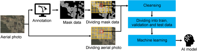
Schematic showing the flow for generating a model for the automatic detection of ridge areas
-
①
Annotation process
An annotation process was used to prepare the teaching data to train the automatic detection model to detect planting and ridge areas. Subsequently, mask images of the planting and ridge areas were prepared as a single visible image, after which annotation was conducted.
-
Manual annotation
After loading the aerial photo into QGIS, the polygons of the paddy field and the ridge areas were manually created and the accuracy was visually confirmed after selecting the polygon-making rule (Fig. 5). The created polygons of the forest area and the ridges are shown in Fig. 6.
Fig. 5 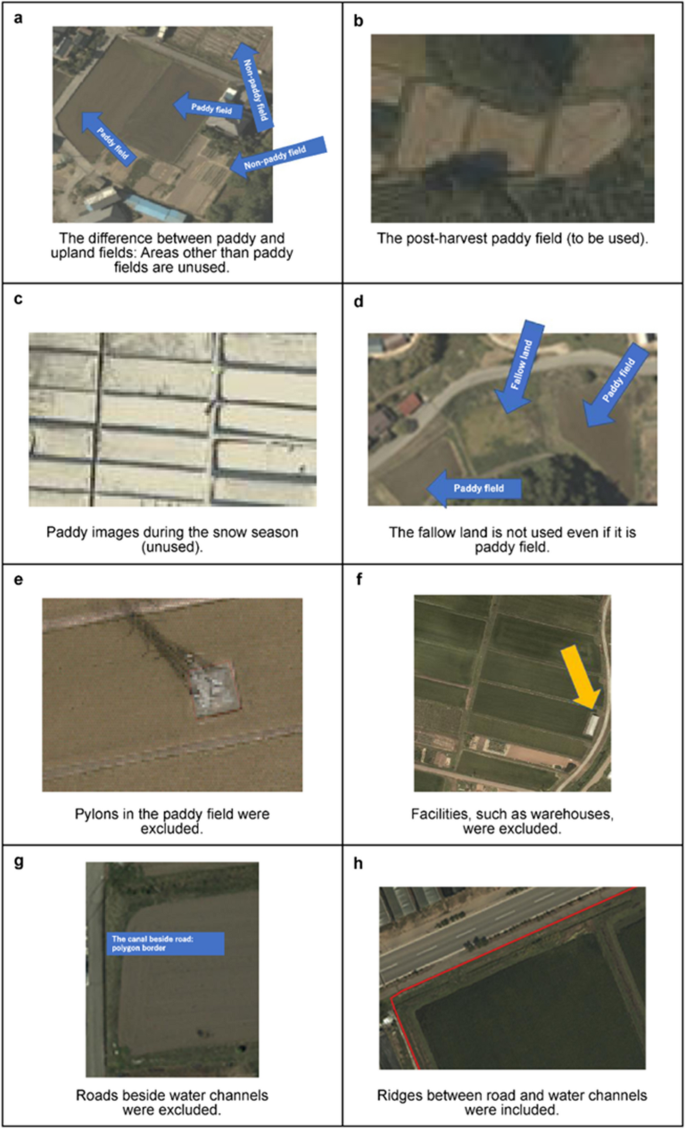
Criteria for creating paddy and planting area polygons for annotation
Fig. 6 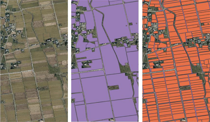
From left to right: Aerial photo, paddy polygon, and planting polygon
-
Semiautomatic annotation
In addition, semiautomatic annotation was conducted only for Area C (Fig. 3a). As a procedure of semiautomatic annotation, 57.3% of the planting areas were automatically extracted, and the planting area polygons were created using aerial photos, the DEM, and MAFF brush polygons. However, the paddy field’s remaining planting areas (42.7%) were manually annotated.
The automatic planting area annotation process was conducted using the following procedure:
-
a.
We extracted only “paddy field” land objects from MAFF brush polygons.
-
b.
We calculated the center-of-gravity coordinate of each brush extracted in a.
-
c.
Next, we mapped the center-of-gravity coordinates calculated in b on the DEM.
-
d.
If the difference between the value of the brush center-of-gravity coordinate (elevation) plotted on the DEM and that of the adjacent pixel was less than a certain value, the adjacent pixel was considered a water-tight area.
-
e.
Based on the flood-filled area pixel detected in d, we further considered neighboring pixels, whose elevation difference from the neighboring pixels was less than a certain value as the flood-filled area. Subsequently, we repeated the process using OpenCV flood-fill (Mallick, 2015). Since the accuracy was inferior to that obtained by manual annotation, cleansing guaranteed the accuracy.
-
-
②
Mask data generation (rasterization)
The conversion of vector data consisting of polygons to raster data consisting of pixels is called rasterization. It is necessary to convert vector data created by manual and semiautomatic annotation into raster data for machine learning. For rasterization, we used the gdal.RasterizeLayer function (GDAL, 2021).
-
③
The division of visible image and mask data
Preprocessing was necessary to create the models (machine training) with FastFCN. Many recent image recognition systems, including FastFCN, use the convolution of images (a CNN method) to extract features from images (Wu et al., 2019). In this process, in many cases, the image size is adjusted (resized, etc.) to fit the structure of the network used in the internal processing. The most common image size used in this study was 4000 × 3000 (pixels), with a maximum size of 8000 × 6000 (pixels), which is relatively large. Additionally, when viewed within a single image, the targeted paddy fields and the areas between rice fields were very small. In addition to the fact that efficient learning cannot be performed with such images, a risk that the accuracy of detecting narrow ridges can be reduced by resizing the images was also observed. This study also divided the aerial photos to be used in advance and used data of a size close to the image size handled by FastFCN. It was considered that the unnecessary training (cleansing, described later) regions could be eliminated and the effects of resizing could be suppressed.
During the pretrial, three patterns with 300 × 300, 400 × 400, and 500 × 500 pixels were evaluated, after deciding the adoption of the 300 × 300 pixel size as the base size because it performed better in both learning efficiency and accuracy (Table 3). Furthermore, since the used aerial photos had some invalid areas (painted white or black according to the photograph’s specifications), we painted the black areas white under certain conditions as part of preprocessing.
Table 3 Class IoU comparison based on image sizes (prevalidation) When the base aerial photo was divided into 300 × 300-pixel images, a point (upper left) of the image (X, Y) = (0, 0) was used as the reference point, after which the following procedure was conducted:
-
a.
Calculation of the number of divisions and shift quantities in the horizontal direction (X coordinate) and vertical direction (Y coordinate)
-
•
Calculation of the number of divisions
Divide the vertical and horizontal sizes of the original image by 300 and round up if it is indivisible (see example below).
$${\text{Original image}}:{ 3}000 \times {3}000{\text{ pixels }} = { 3}000/{3}00{\text{ horizontal}} \times {3}000/{3}00{\text{ vertical }} = { 1}0{\text{ horizontal}} \times {1}0{\text{ vertical divisions}}$$$${\text{Original image}}:{ 4}000 \times {3}000{\text{ pixels }} = { 4}000/{3}00{\text{ horizontal}} \times {3}000/{3}00{\text{ vertical }} = { 13}.{33 }\,( {{14}} ){\text{ horizontal}} \times {1}0{\text{ vertical divisions}}$$-
Calculation of the shift amount
If the vertical and horizontal sizes of the original image are indivisible by the division size of 300 pixels, the image is output with overlapping part(s) in the image. The shift amount for this is calculated as follows.
-
b.
An output image of 300 × 300 pixels, shifting from the reference point (the split position is added to the file name).
-
•
Starting point: upper left corner of the image
Shift amount = Original image width (pixels)/300 (pixels)
$$c=image\, crop\, size$$$$w=base \,image\, width$$$$y = \left[ \frac{w}{c} \right]$$$$Slide\, size = \frac{cy - w}{{\left[ \frac{w}{c} \right]}}$$ -
a.
-
④
Cleansing of images used for machine learning (visual check)
Cleansing extracts the images that can be used as teaching data for machine learning from the images that were divided into 300 × 300 pixels by the previous process. Cleansed data and teaching data are used to train the model for the automatic detection of ridge and planting areas. The accuracy of the results varies depending on the quality and quantity of the data. Cleansing is a task to ensure data quality, and incorrectly annotated images or those that do not contain paddy fields are visually checked and removed. The criteria for judging the images to be removed by cleansing are explained in Fig. 7, where visible and annotated images are placed on the left and right. The numbers of images before and after cleansing are also shown in Table 4. Hence, 4380 annotated images were used to create the teaching data to be input into the model.
Fig. 7 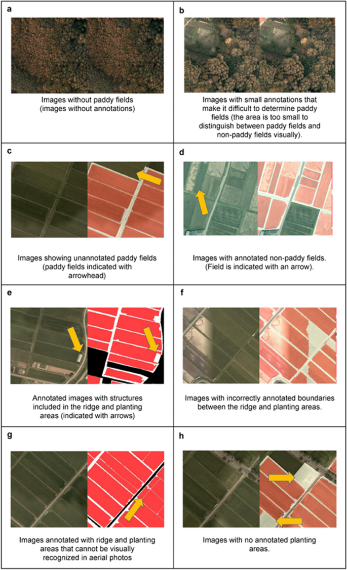
Criteria for image removal in cleansing. Left: aerial photos, right: annotated image (b, c, d, f, and h are combined with their visible images)
Table 4 The amounts of teaching data before and after cleansing -
⑤
Model generation (Training)
-
Organizing teaching data
The teaching data used in FastFCN needed to be divided into the training data used for training, validation data used for verifying the model’s accuracy during training, and test data used to evaluate the completed AI model. Since the amount of teaching data and the total number of images used in this study was approximately 4,000, we adopted a commonly used ratio of training, validation, and testing as follows:
$${\text{Training}}:{\text{Validation}}:{\text{Test }} = { 8}:{1}:{1}$$Then, we randomly sorted the images according to this ratio. Table 5 shows the number of data points by area and the overall data used for the final version of training. The module of the detection model for the planting and ridge areas addressed in this study was created based on the change module (ade20k) (Wu et al., 2019).
Table 5 Amount of training, validation, and test data by area -
Data expansion content
Since the data augmentation method is frequently used to improve the accuracy of machine learning in image recognition, we implemented the augmentation approach shown in Table 6. Data augmentation is applied just before procuring the images as teaching data so that the same images are not used for training every epoch. Therefore, the number of images for training depends on the number of epochs. Since the images were aerial photographs and the orientation was unimportant, upside-down and rotation processes were also performed. The adaptation rate is the percentage of the extended image according to the rate. However, the range of values is the parameter range specified in the image processing library used internally. Therefore, random values were used in both cases. Then, these expansion processes were conducted sequentially to obtain a single image. Moreover, since both the rate of adaptation and the range of values were random, generating images with many variations was also possible. When an image was enlarged, it was cropped to 300 × 300 pixels, which was the base size for training. Similarly, the masked images were also rotated, resized, and cropped. However, the masked images were not subjected to any image processing that would affect the color (color map or grayscale) due to the characteristics of the class specification of the teaching data. Additionally, although the visible image was resized using the [BILNEAR] algorithm, the mask image was resized during the image resizing process using the [NEAREST] algorithm so that the adopted intermediate color was not generated.
Table 6 Expansion method criteria for image recognition data -
Machine Learning Implementation
We set up the learning environment (ABCI environment) for machine learning using the following:
-
GPU NVIDIA V100 for NVLink 16 GiB HBM2 × 4 (max)
-
CPU Intel Xeon Gold 6148 Processor 2.4 GHz
-
CUDA 11.2
Then, machine learning was conducted using the parameters shown in Table 7 as the learning conditions (hyperparameters).
Table 7 Parameter settings for machine learning -
-
-
①
-
(2)
Validation and the use of generated models (inference)
The model generated in process (1) was used to detect the planting area, paddy field areas, and ridge areas. The flow for making the model recognize the visible image to be inferred and creating the polygon data is shown below (Fig. 8). First, (a) the visible image to be inferred was prepared. Then, (b) the image of the target area was divided. The divided image was subsequently inferred using the model trained in (c). Afterward, the masked images of the planting area, forest area, and other areas were released as outputs. Finally, (d) the output masked images were combined, after which (e) three shapefiles of the “planting area,” “paddy field area,” and “ridge area” were released as outputs (vectorization). The parameters used during the recognition process are shown in Table 8.
Fig. 8 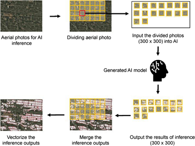
Inference flow of ridge and planting area recognition using the model and DEM
Table 8 Parameter settings for recognition -
(3)
Evaluation of the ridge and planting areas automatically detected by the model
The result of the automatic detection of the ridge and planting areas by the model was expressed by categorizing the detected areas. The categories were divided into areas that can be created when the annotated ridge areas and the ridge areas automatically detected by the model are superimposed into four areas. The detected areas were used to evaluate the accuracy of the automatic detection result of the ridge and planting areas. The accuracy evaluation was conducted using the test data annotated by the operators, as mentioned in Table 5, and by comparing the results detected by the model from the aerial photo on the same test data. TP (true positive) was defined as when the actual ridge area was correctly detected as a ridge area. FP (false positive) is defined as when the nonridge area was incorrectly detected as ridge area. FN (false negative) indicates an undetected ridge area. However, TN (true negative) indicated an area where a nonridge was correctly detected as a nonridge area.
Subsequently, using the indices in Table 7, the recall, precision, false positive rate, F-measure, and intersection over union (IoU) were calculated by using Eqs. (1)–(5) below to confirm the accuracy of the automatic detection of ridge and planting areas. Each value was in the range of 0 to 1, and the closer to 1 the value was, the higher the accuracy.
$$\mathrm{Percentage \,of\, correct\, answers }\,(\mathrm{Accuracy}) =\frac{TP+TN}{TP+TN+FP+ FN}$$(1)$$\mathrm{Recurrence\, rate }\,(\mathrm{Recall}) = \frac{TP}{TP+FN}$$(2)$$\mathrm{Precision }=\frac{TP}{TP+FP}$$(3)$$\mathrm{F}-\mathrm{measure }=2*\frac{\mathrm{Precision }*\mathrm{ Recall }}{\mathrm{Precision}+\mathrm{Recall}}$$(4)$$\mathrm{IoU }=\frac{TP}{TP+FP+ FN}$$(5)The percentage of correctness in Eq. (1) is the percentage of the area that the model correctly detected out of the total area of the evaluated image (the sum of the areas correctly detected as ridge and nonridge areas). The recall in Eq. (2) is the percentage of the area that the model correctly detected as ridge areas out of the actual total ridge area. When this value is high, the model misses few ridge areas. In Eq. (3), the precision is the area’s rate, that is, the actual ridge area out of the area that the model detected as the ridge area. When this value is high, the area detected as a nonridge area instead of a ridge area by mistake is small. The F-measure in Eq. (4) is the harmonic mean of the reproduction and conformity rates. It is expressed as one value and considers both the reproduction and conformity rates, which have complementary properties to each other. Finally, the IoU in Eq. (5) is an index representing the degree of overlap between the actual ridge area and the area detected by the AI model. The IoU is a value obtained by dividing the common area by the sum set. Figure 9 illustrates its calculation.
Fig. 9 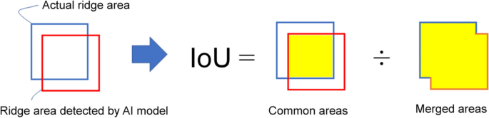
Method for calculating the IoU
-
(4)
Accuracy assessment of the slope, ridge areas, and ridge rate based on mask images
The accuracy of the real ridge areas calculated with the slope data and ridge rate were also evaluated. The sample data for comparisons were extracted from the mask images of planting and ridge areas, the mask images in the test data prepared during model generation (training), as previously mentioned in Table 5, and the mask images automatically detected by the model.
-
Measurement of the planting and ridge area (m2) as horizontally projected areas
The mask images in the test data during model generation (training) and the mask images automatically detected by the model can be input into QGIS as raster data. “Zone statistics” in “raster analysis” of the “processing toolbox” can be used to calculate the areas as horizontally projected areas.
-
Measurement of the slope and ridge areas (m.2)
Precise elevation data were discriminated for each 0.5 m mesh (0.25 m2). It was then possible to calculate the slope from the elevation difference in the ridge. Subsequently, QGIS converted the elevation raster data into slope raster information for each mesh using the slope calculation function of raster analysis. “Zone statistics (raster)” in raster analysis of the processing toolbox were used to calculate the average slope of the ridge in the ridge mask. Then, the result was displayed as the “mean” in the attribute table of raster analysis results. Finally, the real ridge area was calculated using the trigonometric formula (the horizontally projected area ÷ cosθ).
-
Calculation of the ridge rate
The ridge rate in the paddy fields was calculated by dividing by the sum of the planting areas and the real ridge area.
$${\text{Ridge rate }} = {\text{ Real ridge area}}/ \, \left( {{\text{Planting area }} + {\text{ Real ridge area}}} \right) \times { 1}00$$
-
-
(5)
Generating planting and ridge polygons for the entire Nagano Prefecture
First, the trained model was applied to the available aerial photos of the entire Nagano Prefecture to produce planting and ridge area polygons. The planting areas, ridge slope and ridge areas, and ridge rates were measured and calculated from the polygonised inference results and the DEM (Nagano Forestry General Center, 2021).
-
Measurement of the planting area (m2)
Assuming that the slope in the planting area can be neglected, the area of each land object could then be calculated based on the planting area polygon layer attribute table using the field calculator “Geometry: $area” in QGIS.
-
Measurement of the slope and ridge areas (m2)
QGIS converted the elevation raster data into slope raster information using the slope calculation function of raster analysis. “Zone statistics (vector)” in the raster analysis of the processing toolbox was used to calculate the average slope of the ridge from the slope information of all the meshes that existed in the ridge polygon partition. Then, the result was displayed as “_mean” in the attribute table of the ridge polygon layer. Finally, the area on the map of each ridge polygon was calculated as a horizontally projected area using the $area function of the geometry and field calculator in the attribute table. The real area of the ridge was calculated using the trigonometric formula (the horizontally projected area/cosθ). The ridge rate was calculated as previously stated in (4).
-


Results
Accuracy evaluation of the ridge and planting areas automatically detected by the AI model
The accuracy evaluation of the detected ridge and planting areas using the model in the six areas, A to F, in Fig. 2b is shown in Table 9. The model detected ridge and planting areas with accuracies of 96.41% and 96.30%, precision scores of 84.76% and 94.45%, recall scores of 82.20% and 94.45%, F-measure values of 83.46% and 94.45%, and IoU scores of 71.62% and 89.48%, respectively.
The right figure in Fig. 10 shows the model superimposition of the ridge areas of the training and detection data. The red area denotes where they matched completely, while the blue areas denote where the model failed to detect ridges. However, the green areas denote where nonridge areas were detected as ridges. Compared with the planting areas, the IoU value of the ridge areas decreased during the calculation even at the same paddy field since the ridge areas were much narrower than the planting areas.

Diagram showing an IoU example of actual evaluation data
It was hypothesized that increasing the quantity and quality of the training data could increase the value of the IoU in ridge areas. Multiple linear regression was calculated to identify the factors that could increase the IoU based on the amount of training data and their resolutions. As a result, a significant regression equation was not found for the ridge areas of all 6 surveyed areas. Table 9 shows that the IoU value of area C was 52.44%, which was lower than that of the other 5 areas. It was assumed that the occurred because the teaching data were generated semiautomatically, while the data of other areas were generated by manual annotation. Thus, multiple linear regression was calculated without area C, and the significant regression equation in (2) is shown in Table 10. This result suggested that the accuracy increases when the amount of training data with higher resolution under the suggested manual annotation is increased. For the results of (3) in the planting areas, a significant regression equation for describing the training data and the IoU was not obtained. On the other hand, a significant regression equation was obtained through a single regression analysis of the average planting area size of each paddy field and the IoU (R2 = 0.8176, P = 0.013). This result indicated that the differences in the IoU of the planting areas could be caused by the sizes of the paddy fields. Area B and E had lower IoU values (86.13% and 86.94%) than the other areas did. Its reason could be assumed because paddy fields in area B and E tend to be smaller mostly located in the hilly and mountainous areas. It was assumed that the model reached a high IoU in planting areas with a smaller amount of training data.
Accuracy evaluation of the ridge areas with the slope data and ridge rates
Table 11 compares the planting area, ridge slopes, real ridge areas, and ridge rates in the paddy fields measured from the mask images as test data during model generation (training) and the mask images automatically detected by the model. As shown, the difference between them was − 0.34% for the planting area, 5.61% for the real ridge area, and 4.76 ppt for the ridge rate. Given that the training data were generated semiautomatically in Area C, Tables 9, and 10 show that the ridge areas in Area C have lower accuracies than the other areas.
Ridge and planting area polygons detected using the models of the entire Nagano Prefecture
Using the model generated by machine learning, the polygons of the planting and ridge areas in the paddy farmland of the entire Nagano Prefecture were created by recognizing aerial images from the entire Nagano Prefecture. A total of 3660 images of 4000 × 3000 pixels and 287 images of 8000 × 6000 pixels were obtained with aerial photography of the Nagano Prefecture. As shown in Fig. 8, these images were divided into 300 × 300 aerial photos, with the former divided into 180 and the latter into 690, resulting in 856,830 divided images that the model recognized. Figure 11 shows the polygons of the planting and ridge areas created from the images of each area in Nagano Prefecture. The areas were calculated via QGIS with AI-created polygons and a DEM; there were 283 million m2 of planting areas and 70 million m2 of the ridge areas, and the ridge rate was 19.85% (Table 12). Among the nine regions of the prefecture, the Kiso and Shimoina regions had ridge rates that were more than 30%, which were the highest among the areas. The total time required for output generation of the mask images and merging them (the planting/ ridge areas, paddy fields) using model inference from the division of aerial photographs was approximately 256 h, and the vectorization process of the merged images took approximately 3 h. The calculation of the areas from the polygon required approximately 36 h. In total, 2–3 weeks of work was needed for these steps.

AI-generated planting area and bedside polygons
Discussion
Measurement results of the planting and ridge polygon areas, the ridge slope, and the ridge rate detected by the model
This study showed that the model generated using the machine learning approach proposed in this study can automatically detect the planting and ridge areas of paddy fields from aerial images of farmland with an accuracy of more than 96% and can create polygons that can be used in GIS. Furthermore, the area of the planting polygon, the slope angle of the ridge, the accurate area of the ridge polygon, considering its slope angle, and the ridge rate could be measured in GIS using a precision DEM. Based on the time required to obtain these data, it was possible to measure the recognition of farmland images using the model, create polygons for the planting and ridge areas, calculate areas and slopes by a DEM, and calculate the ridge rates for paddy areas throughout Nagano Prefecture in approximately 2 to 3 weeks.
From the differences in the values of the mask images for test data (training) and the mask images detected by the model, it was possible to calculate the ridge area and the ridge rate maximum errors of 5.61% and 4.76%, respectively. Hamano et al. (2022) calculated the root-mean-square error at 1.96° of the ridge slope measured from the ridge polygon created by QGIS and a DEM prepared for Nagano Prefecture, and the actual measurement in the field was 1.96°. The error of the ridge area can be calculated at approximately 1.2% for a slope of 20° and 1.9% for a slope of 30°. Combining both errors, it is necessary to consider a maximum error of 7.8% to 8.5%. There is still room to improve the accuracy of the model in detecting ridge areas. According to the discussion above (Tables 10 and 11), the model prepared in this study can detect ridge areas with high accuracy and improve the IoU by 71% by increasing the training data during annotation.
Possibility of using the planting area and ridge polygons created in this study
Reducing the cost and labor burden of mowing in ridge areas of paddy fields is important, especially in hilly and mountainous regions (Kito et al., 2011). Hence, it is necessary to analyze farm management, including the labor efficiency and cost-effectiveness of introducing machines, by calculating the break-even point. The ridge area and slope information are fundamental to determine the labor and fuel costs based on simulating the working time required for mowing by using the different types of mowing machines (Uehara et al., 2021). The polygons of the planting and ridge areas of the entire Nagano Prefecture created in this research were made available as online open data. Therefore, these polygon data can be downloaded and used in GIS software. Using these polygons and the open precision DEM of Nagano Prefecture, it will be possible to measure planting areas, ridge slopes, real ridge areas, and ridge rates by combining and dividing them according to the necessary analysis content (Hamano et al, 2022). Since the ridge polygons have been created across two or more paddy fields in each paddy field zone, each polygon can be divided in GIS according to the land possessed or rented by a farmer so that they can analyze the ridge mowing costs within their cultivation budget. If a farmer aims to examine the movable range of a remote control grass mowing machine according to the specification on the possible angle of the ridge surface, the average and maximum slope angles on long- and short-side ridges can be calculated by further dividing the ridge polygons. For local governments, an effective subsidy distribution method to support rice cultivation in hilly and mountainous areas (MAFF, 2020a) can be realized by introducing ridge area and ridge rate information. Since paddy fields with larger and steeper ridges have higher costs, especially for mowing work, appropriate budget allocation can be considered by utilizing ridge data.
How to use the model in regions outside Nagano Prefecture
Studies have proposed developing models similar to the one in this study as open source models. Therefore, it will be possible to create planting areas and ridge polygons by running the program using available farmland images in regions other than Nagano Prefecture. Furthermore, when the model generated in this study is used, a possibility exists that the accuracy of detecting the planting and ridge areas will be different from the results in this study depending on the amount and quality of the visible images used. Nevertheless, precise elevation data should be prepared for slope measurement in each prefecture since not all local governments have obtained precise elevation data, such as in Nagano Prefecture. Moreover, in addition to aerial laser surveying data, satellite data and drone imaging data could be used to reasonably obtain a precise DEM.
Conclusion
This study generated a model to detect ridge and planting area polygons in paddy fields by applying machine learning from annotated polygons that distinguished ridge and planting areas on aerial images. Subsequently, the polygons created by the model allowed us to measure the planting areas and ridge areas with ridge slope data from the DEM on GIS software. It was identified that the accuracy of ridge area detection can be improved by increasing the amount of annotated training data. Information on ridge slopes and areas can simulate the availability and efficiency of new machinery for reducing the burden of mowing work based on technical and economic evaluations. Furthermore, ridge rate information can be used to help evaluate labor productivity and land productivity, including mowing machinery and labor costs. As a result, these data can support farmers and agricultural corporations in calculating their farming costs accurately with labor costs and machinery efficiency to reflect their farm management efforts, especially in hilly and mountainous areas. Furthermore, to generalize the model to ridge and planting area polygons in other areas, the accuracy of the model created in this study should be examined with different farm-area photographs using satellites and drones. Since not all local governments have obtained precise elevation data, reasonable methods should be examined with aerial laser surveying and satellite or drone imaging information.
Data availability
None.
Code availability
None.
References
Ando, M. (1996). New development of regional farming groups: beyond production (pp. 22–44). Japan Agricultural Statistics Association.
Arita, H., & Kimura, K. (1993). On the influences of paddy field shape to levee weeding labor developing farm land consolidation technique in regarding to labor efficiency of levee weeding (I). Transactions of the Japanese Society of Irrigation, Drainage and Reclamation Engineering, 163(2), 87–94.
GDAL. gdal_rasterize. (2021). Program in GDAL documentation. GDAL.
Hamano, M., Kitaki, Y., Kurata, Y., & Watanabe, O. (2022). Development of measuring method of paddy field ridges in hilly and mountainous areas: Application of geographic information system software and precision digital elevation data (DEM). Japanese Journal of Farm Work Research, 57(1), 41–48.
Ito, J., Feuer, N. H., Kitano, S., & Asahi, H. (2019). Assessing the effectiveness of Japan’s community-based direct payment scheme for hilly and mountainous areas. Ecological Economics, 160, 62–75. https://doi.org/10.1016/j.ecolecon.2019.01.036
Kawasaki, K. (2010). The costs and benefits of land fragmentation of rice farms in Japan. The Australian Journal of Agricultual and Resource Economics, 54(4), 509–526. https://doi.org/10.1111/j.1467-8489.2010.00509.x
Kito, I., Awaji, K., & Miura, S. (2010). Evaluation of weeding work cost on paddy field levees in the hillside. Japanese Journal of Farm Management, 48(1), 67–72. https://doi.org/10.11300/fmsj.48.1_67
Kito, I., Awaji, K., & Miura, S. (2011). Large scale rice farm’s strategy for weed working in hilly and mountainous area. Japanese Journal of Farm Management, 49(3), 67–72. https://doi.org/10.11300/fmsj.49.3_67
Ministry of Agriculture, Forestry and Fisheries (2020b). Provision and utilization of agricultural land information (farm plot polygon), Ministry of Agriculture. https://www.maff.go.jp/j/tokei/porigon/.
Ministry of Agriculture, Forestry and Fisheries (2020c). Successful determination of agricultural land shape by AI: Shortening the updating period of farm plot polygon from 5 year to 1 year. https://www.maff.go.jp/j/press/tokei/kikaku/200710.html
Ministry of Agriculture, Forestry and Fisheries (2020a) Summary of the Basic Plan for Food, Agriculture and Rural Areas, Ministry of Agriculture, Forestry and Fisheries, 40p. https://www.maff.go.jp/e/policies/law_plan/attach/pdf/index-13.pdf
Ministry of Agriculture, Forestry and Fisheries (2022) Area survey in crop statistical survey (in Japanese), Ministry of Agriculture, Forestry and Fisheries. https://www.maff.go.jp/j/tokei/kouhyou/sakumotu/menseki/index.html#y
Mallick, S. (2015). Filling holes in an image using OpenCV (Python/C++). LearnOpenCV.
Nagano Forestry General Center (2021). Nagano prefecture_0.5_mDEM, G-spatial information center. https://www.geospatial.jp/ckan/dataset/nagano-dem.
Onojeghuo, A. O., Blackburn, G. A., Wang, W., Atkinson, P. M., Kindred, D., & Miao, Y. (2018). Mapping paddy rice fields by applying machine learning algorithms to multi-temporal Sentinel-1A and Landsat data. International Journal of Remote Sensing, 39(4), 1042–1067. https://doi.org/10.1080/01431161.2017.1395969
Oyoshi, K., Tomiyama, N., Okumura, T., Sobue, S., & Sato, J. (2016). Mapping rice-planted areas using time-series synthetic apertureradar data for the Asia-RiCE activity. Paddy and Water Environment, 14(4), 463–472. https://doi.org/10.1007/s10333-015-0515-x
Pramanik, M. K. (2016). Site suitability analysis for agricultural land use of Darjeeling district using AHP and GIS techniques. Modeling Earth Systems and Environment. https://doi.org/10.1007/s40808-016-0116-8
Qiu, Z., Chen, B., & Takemoto, K. (2014). Conservation of terraced paddy fields engaged with multiple stakeholders: The case of the Noto GIAHS site in Japan. Paddy and Water Environment, 12, 275–283. https://doi.org/10.1007/s10333-013-0387-x
Sharma, A., Jain, A., Gupta, P., & Chowdary, V. (2020). Machine learning application for precision agriculture: a comprehensive review. IEEE, 9, 4843–4873.
Statistics Bureau of Japan (2022) Crop statistical survey (in Japanese) in e-Stat, Statistics Bureau of Japan. https://www.e-stat.go.jp/stat-search/files?page=1&layout=datalist&toukei=00500215&tstat=000001013427&cycle=7&tclass1=000001032270&tclass2=000001032271&tclass3=000001163069&cycle_facet=tclass1%3Atclass2%3Atclass3&tclass4val=0
Takeyama, K., Yamamoto, Y., & Abe, S. (2013). Weed control for TaU border ridges of rice paddy in Shimane-Prefecture: Overcoming aging-farmer trends through cooperative efforts of group farming corporations. Bulletin of the Shimane Agricultural Technology Center, 41, 19–34.
Toda, K. (2012). Preparation of microtopographic maps using aerial laser survey data. Journal of Japan Society Erosion Control, 65(2), 51–55. https://doi.org/10.11475/sabo.65.2_51
Toda, K. (2019). Advancement of investigation method of collapse mechanism by laser surveying. Research Reports, Nagano Forestry Research Center, 33, 1–8.
Uchikawa, Y., Matsui, M., Arase, T., & Tamura, T. (2018). Safety and efficiency for weeding work and levee slope’s form required for mowing machines on paddy fields in steep sloping areas in Japan. International Journal of GEOMATE, 14(42), 20–24. https://doi.org/10.21660/2018.42.7128
Uehara, Y., Iizuka, K., & Iwano, Y. (2021). The importance of ridge management and development of mowing machine on ridge and slope in Nagano Prefecture. System, Control, and Information Engineers, 65(12), 471–476. https://doi.org/10.11509/isciesci.65.12_471
Wu, H., Zhang, J., Huang, K., Liang, K., & Yu, Y. (2019). FastFCN: rethinking dilated convolution in the backbone for semantic segmentation. https://arxiv.org/abs/1903.11816.
Wu, H. (2020). wufukai/FastFCN, GitHub. https://github.com/wuhuikai/FastFCN.
Wu, B., Wu, Y., Aoki, Y., & Nishimura, S. (2020). Mowing patterns comparison: analyzing the mowing behaviors of elderly adults on an inclined plane via a motion capture device. IEEE, 8, 216623–216633. https://doi.org/10.1109/ACCESS.2020.3040418
Yagi, H. (2009). Labor input allocation for farmland conservation in thehilly and mountainous areas: Estimation with census agriculturalsettlements cards. J Rural Plan Assoc, 28(4), 405–411. (in Japanese).
Zhao, Z., Benoy, G., Chow, T. L., Rees, H. W., Daigle, J., & Meng, F. (2010). Impacts of accuracy and resolution of conventional and LiDAR based DEMs on parameters used in hydrologic modeling. Water Resources Management, 24(7), 1363–1380.
Acknowledgements
This study was jointly implemented by the research team of Shinshu University (Faculty of Agriculture), who has been studying the measurement of paddy field ridge areas and management costs in hilly and mountainous areas with GIS and a DEM, and the research team of Recruit Co., Ltd. (Advanced Technology Lab.), who has provided AI and image processing technology. The DEM and aerial photos for this study were provided by the Nagano Forestry Center, Nagano Prefecture. This research did not receive any specific grant from funding agencies in the public, commercial, or not-for profit sectors.
Funding
None.
Author information
Authors and Affiliations
Contributions
Conceptualization: [MH], [SY], [OW], [SS]; methodology on AI/machine learning/image processing:[SS], [SY], [NS], and on GIS/DEM/Agricultural land analysis:[MH], [YK], [OW]; formal analysis and investigation on AI/machine learning/image processing: [SS], [SY], [NS], and on GIS/DEM/agricultural land measure: [MH], [YK]; writing—original draft preparation on AI/machine learning/image processing: [SY], [NS], and on GIS/DEM/Agricultural land analysis: [MH]; writing—review and editing on AI/machine learning/image processing: [SS], [SY], [NS] and on GIS/DEM/Agricultural land analysis: [MH], [YK], [OW]; supervision: [OW], [SS].
Corresponding author
Ethics declarations
Competing interest
The authors have no conflicts of interest to declare.
Ethical approval
None.
Informed consent
None.
Additional information
Publisher's Note
Springer Nature remains neutral with regard to jurisdictional claims in published maps and institutional affiliations.
Rights and permissions
Open Access This article is licensed under a Creative Commons Attribution 4.0 International License, which permits use, sharing, adaptation, distribution and reproduction in any medium or format, as long as you give appropriate credit to the original author(s) and the source, provide a link to the Creative Commons licence, and indicate if changes were made. The images or other third party material in this article are included in the article's Creative Commons licence, unless indicated otherwise in a credit line to the material. If material is not included in the article's Creative Commons licence and your intended use is not permitted by statutory regulation or exceeds the permitted use, you will need to obtain permission directly from the copyright holder. To view a copy of this licence, visit http://creativecommons.org/licenses/by/4.0/.
About this article

Cite this article
Hamano, M., Shiozawa, S., Yamamoto, S. et al. Development of a method for detecting the planting and ridge areas in paddy fields using AI, GIS, and precise DEM. Precision Agric 24, 1862–1888 (2023). https://doi.org/10.1007/s11119-023-10021-z
Accepted:
Published:
Issue Date:
DOI: https://doi.org/10.1007/s11119-023-10021-z