
Abstract
This research investigates the utilization of a modified version of the Sardar sub-equation method to discover novel exact solutions for the generalized Pochammer Chree equation. The equation itself represents the propagation of longitudinal deformation waves in an elastic rod. By employing this modified method, we aim to identify previously unknown solutions for the equation under consideration, which can contribute to a deeper understanding of the behavior of deformation waves in elastic rods. The solutions obtained are represented by hyperbolic, trigonometric, exponential functions, dark, dark-bright, periodic, singular, and bright solutions. By selecting suitable values for the physical parameters, the dynamic behaviors of these solutions can be demonstrated. This allows for a comprehensive understanding of how the solutions evolve and behave over time. The effectiveness of these methods in capturing the dynamics of the solutions contributes to our understanding of complex physical phenomena. The study’s findings show how effective the selected approaches are in explaining nonlinear dynamic processes. The findings reveal that the chosen techniques are not only effective but also easily implementable, making them applicable to nonlinear model across various fields, particularly in studying the propagation of longitudinal deformation waves in an elastic rod. Furthermore, the results demonstrate that the given model possesses solutions with potentially diverse structures.
1 Introduction
In order to explore the properties and traits of nonlinear models found in nonlinear science, thorough investigation is necessary. Nonlinear science encompasses a vast array of disciplines, including chaos theory, fractals, complex systems, and nonlinear dynamics. These models exhibit behaviors that are not easily predictable or linearly related to their inputs, making them particularly intriguing and challenging to study. By delving into the intricacies of these nonlinear models, researchers can gain valuable insights into the complexity and interconnectedness of natural phenomena, leading to a deeper understanding of our world and its underlying dynamics. A crucial area of focus lies in the in-depth exploration of the propagation of nonlinear waves, particularly emphasizing their behavior within multilayered bodies. This subject is essential for a thorough analysis and understanding of the intricate dynamics and properties associated with the transmission of nonlinear waves in the context of layered materials. Through a meticulous examination of these phenomena, the goal is to furnish a comprehensive understanding of the distinctive challenges and complexities inherent in the propagation of nonlinear waves within multilayered structures. These investigations significantly contribute to the advancement of our knowledge in this field, offering insights into the subtle interactions and dynamics that govern the propagation of nonlinear waves across various material configurations. Nonlinear partial differential equations pose significant challenges when it comes to finding analytical solutions. These equations involve nonlinear terms that make it difficult to employ conventional methods for solving linear partial differential equations. As a result, researchers have developed various techniques to tackle these nonlinear equations, including numerical methods, perturbation methods, integral transforms, and more. While exact analytical solutions are often elusive for nonlinear partail differential equations (NPDEs), approximate solutions or qualitative insights can still be obtained through these methods. Nonlinear partial differential equations are challenging to solve analytically, and various methods have been developed to obtain exact or approximate solutions. Some commonly used techniques include the \(\phi ^6\)-model expansion technique (Ullah et al. 2023; Isah and Yokus 2022; Isah 2023; Yao et al. 2023; Ali et al. 2022; Sadaf et al. 2022), The Kudryashov method (Murad et al. 2023; Malik et al. 2023; Cinar et al. 2023; Esen et al. 2023), the Hirota bilinear method (Ismael et al. 2023; Yokus and Isah 2023; Mandal et al. 2023; Batool et al. 2023; Seadawy et al. 2021; Yokus and Isah 2022; Ismael and Sulaiman 2023; Ali et al. 2023), the extended simplest equation method (Murad et al. 2023; Zayed and Shohib 2019; Ahmed et al. 2021; El Sheikh et al. 2020; Hassan and Altwaty 2020), and other methods (Ali et al. 2023; Kamal Ali et al. 2022; Ismael et al. 2023, 2023; Ali et al. 2023, 2023; Zhu et al. 2021; Isah and YOKUS 2022; Günerhan et al. 2020; Zayed and El-Ganaini 2024; Al-Amr 2015; El-Ganaini et al. 2023; Mubaraki et al. 2024; Asif et al. 2023a, b; Mubaraki et al. 2023; Mahdy 2023, 2022; Mahdy et al. 2022; Al-Bugami et al. 2023; Mahdy et al. 2023, 2022; Mahdy and Mohamed 2022; Mahdy et al. 2023; Anaç 2023). In this study, we will employ the modified version of the Sardar sub-equation method (MSSEM) as our chosen approach. Extensive research has been conducted on this particular method, with numerous studies dedicated to its exploration and analysis. Akinyemi et al. conducted a comprehensive investigation of the unstable nonlinear Schrödinger equation when generalized to incorporate the mentioned method (Akinyemi et al. 2022). Another research endeavor focused on the examination of optical solitons utilizing the mentioned method (Cinar et al. 2022). The method was applied to the space-time fractional modified third-order Korteweg-de Vries equation to investigate soliton solutions in a research study (Rehman et al. 2022). Numerous studies have been conducted on this method, encompassing a wide range of equations and employing diverse approaches. These investigations have delved into various aspects and applications, contributing to a comprehensive understanding of the method’s effectiveness and versatility in different contexts (Ullah et al. 2023; Rehman et al. 2022; Asjad et al. 2022; Onder et al. 2023; Yao et al. 2023; Akinyemi et al. 2021; Yusuf et al. 2022; Faisal et al. 2023; Akinyemi 2021; Alia et al. 1402; Muhammad et al. 2022). In this particular study, our focus will be on utilizing the generalized Pochhammer–Chree equation as the primary equation of interest. We applied the modified Sardar sub-equation method to construct some novel solutions. The Pochhammer-Chree equation, introduced by Clarkson et al. in (1986), represents the propagation of longitudinal deformation waves in an elastic rod. It is mathematically described as follows:
where the function u(x, t) represents the longitudinal displacement at time t of a material point that was initially located at position x. It serves as a fundamental quantity for studying the behavior and dynamics of the deformation waves within the elastic rod (Clarkson et al. 1986). Bogolubsky successfully obtained soliton-type solutions by considering various values of n, specifically \(n = 2, 3, and 5\). These solutions offer valuable insights into the behavior and characteristics of solitons within the context of the Pochhammer–Chree equation (Bogolubsky 1977). Exact solutions have been acquired by Triki et al. for \(n = 6\) (Triki et al. 2015). The generalized Pochhammer–Chree equation is given by Yokus et al. (2022), Parand and Rad (2010)
where \(\mu \), \(\beta \) and v are constants. The Pochhammer-Chree equation has been extensively investigated using various methods, for obtaining solitary wave solutions, periodic solutions, kink shape solutions, singular solutions, complex rational function solutions, complex periodic solutions, and so Weiguo and Wenxiu (1999), Liu (1996), Wazwaz (2008), Li and Zhang (2002), Shawagfeh and Kaya (2004), El-Ganaini (2011), Mohebbi (2012), Parand and Rad (2010), Zuo (2010), Zhang (2005), Zhang et al. (2010), Jaradat et al. (2022). These different approaches have been employed to analyze the equation, explore its properties, and obtain meaningful solutions. Each method offers unique advantages and insights into the behavior and dynamics of the equation, contributing to a comprehensive understanding of its mathematical properties.
In this article, we provide an introduction in the previous section. Then, in the second section, we provide an overview of the MSSEM. Next, in the third section, we apply MSSEM to find new exact solutions for The generalized Pochhammer-Chree equation and present them using 3D, 2D, and counter plots. Finally, we conclude our work in the last section.
2 Description of the MSSEM
The Sardar sub-equation method is a powerful technique to obtain exact solutions of nonlinear PDEs (Akinyemi et al. 2022). A recent study proposed a modification version of this method, incorporating arbitrary functions into the trial solution ansatz. The NPDEs is expressed as:
If we consider the following transformation:
The new modification of the Sardar sub-equation method depends on the following function:
where \(\lambda _{i}, (i=0,1,2,...,L)\) are coefficients of \(\mathcal {Q}^{i}(\chi )\) with \(\lambda _{N}\ne 0\) and the following equation exists for the \(\mathcal {Q}(\chi )\) function:
where \(\gamma _{0}\), \(\gamma _{1}\) and \(\gamma _{2}\) are constants. The general solutions Eq. (6) are outlined as follows:
-
1.
When \(\gamma _{0}=0\), \(\gamma _{1}>0\), and \(\gamma _{2}\ne 0\), then
$$\begin{aligned}{} & {} \mathcal {Q}_{1}(\chi )=\pm \sqrt{-\frac{\gamma _{1}}{\gamma _{2}}} \text {sech}[\sqrt{\gamma _{1}}(\chi + \rho )], \end{aligned}$$(7)$$\begin{aligned}{} & {} \mathcal {Q}_{2}(\chi )=\pm \sqrt{\frac{\gamma _{1}}{\gamma _{2}}} \text {csch}[\sqrt{\gamma _{1}}(\chi + \rho )]. \end{aligned}$$(8) -
2.
When \(\gamma _{0}=0\), \(\gamma _{1}>0\), and \(\gamma _{2}= \pm 4 \beta _{1} \beta _{2}\), then
$$\begin{aligned} \mathcal {Q}_{3}(\chi )= \pm \frac{4 \beta _{1} \sqrt{\gamma _{1}}}{\left( 4 \beta _{1}^2 - \gamma _{2}\right) \text {cosh}[\sqrt{\gamma _{1}}(\chi + \chi _{0})]+\left( 4 \beta _{1}^2 + \gamma _{2}\right) \text {sinh}[\sqrt{\gamma _{1}}(\chi + \chi _{0})]}, \end{aligned}$$(9)where \(\beta _{1}\) and \( \beta _{2}\) are constants.
-
3.
When \(\gamma _{0}=\frac{\gamma _{1}^2}{4 \gamma _{2}}\), \(\gamma _{1}<0\), and \(\gamma _{2}> 0 \), with constants \(A_{1}\) and \(A_{2}\), then
$$\begin{aligned} \mathcal {Q}_{4}(\chi )= \pm \sqrt{-\frac{\gamma _{1}}{2 \gamma _{2}}} \text {tanh}\left[ \sqrt{-\frac{\gamma _{1}}{2}}(\chi + \rho )\right] , \end{aligned}$$(10)$$\begin{aligned} \mathcal {Q}_{5}(\chi )= \pm \sqrt{-\frac{\gamma _{1}}{2 \gamma _{2}}} \text {coth}\left[ \sqrt{-\frac{\gamma _{1}}{2}}(\chi + \rho )\right] , \end{aligned}$$(11)$$\begin{aligned} \mathcal {Q}_{6}(\chi )= \pm \sqrt{-\frac{\gamma _{1}}{2 \gamma _{2}}} \left( \text {tanh}[\sqrt{-2 \gamma _{1}}(\chi + \rho )] \pm i \text {sech}[\sqrt{-2 \gamma _{1}}(\chi + \rho )] \right) , \end{aligned}$$(12)$$\begin{aligned} \mathcal {Q}_{7}(\chi )= \pm \sqrt{-\frac{\gamma _{1}}{8 \gamma _{2}}} \left( \text {tanh}\left[ \sqrt{-\frac{\gamma _{1}}{8}}(\chi + \rho )\right] + \text {coth}\left[ \sqrt{-\frac{\gamma _{1}}{8}}(\chi + \rho )\right] \right) , \end{aligned}$$(13)$$\begin{aligned} \mathcal {Q}_{8}(\chi )= \pm \sqrt{-\frac{\gamma _{1}}{2 \gamma _{2}}} \left( \frac{\text {cosh}[\sqrt{-2\gamma _{1}}(\chi + \rho )]}{\text {sinh}[\sqrt{-2\gamma _{1}}(\chi + \rho )]\pm i}\right) . \end{aligned}$$(14) -
4.
When \(\gamma _{0}=0\), \(\gamma _{1}<0\), and \(\gamma _{2}\ne 0 \), then
$$\begin{aligned} \mathcal {Q}_{9}(\chi )= \pm \sqrt{-\frac{\gamma _{1}}{ \gamma _{2}}} \text {sec}\left[ \sqrt{-\gamma _{1}}(\chi + \rho )\right] , \end{aligned}$$(15)$$\begin{aligned} \mathcal {Q}_{10}(\chi )= \pm \sqrt{-\frac{\gamma _{1}}{ \gamma _{2}}} \text {csc}\left[ \sqrt{-\gamma _{1}}(\chi + \rho )\right] . \end{aligned}$$(16) -
5.
When \(\gamma _{0}=\frac{\gamma _{1}^2}{4 \gamma _{2}}\), \(\gamma _{1}>0\), \(\gamma _{2}> 0 \), and \(A_{1}^2- A_{2}^2>0\), then
$$\begin{aligned} \mathcal {Q}_{11}(\chi )= \pm \sqrt{\frac{\gamma _{1}}{ 2 \gamma _{2}}} \text {tan}\left[ \sqrt{\frac{\gamma _{1}}{2}}(\chi + \rho )\right] , \end{aligned}$$(17)$$\begin{aligned} \mathcal {Q}_{12}(\chi )= \pm \sqrt{\frac{\gamma _{1}}{ 2 \gamma _{2}}} \text {cot}\left[ \sqrt{\frac{\gamma _{1}}{2}}(\chi + \rho )\right] , \end{aligned}$$(18)$$\begin{aligned} \mathcal {Q}_{13}(\chi )= \pm \sqrt{\frac{\gamma _{1}}{ 2 \gamma _{2}}} \left( \text {tan}\left[ \sqrt{2\gamma _{1}}(\chi + \rho )\right] \pm \text {sec}\left[ \sqrt{2\gamma _{1}}(\chi + \rho )\right] \right) , \end{aligned}$$(19)$$\begin{aligned} \mathcal {Q}_{14}(\chi )= \pm \sqrt{\frac{\gamma _{1}}{ 8 \gamma _{2}}} \left( \text {tan}\left[ \sqrt{\frac{\gamma _{1}}{8}}(\chi + \rho )\right] - \text {cot}\left[ \sqrt{\frac{\gamma _{1}}{8}}(\chi + \rho )\right] \right) , \end{aligned}$$(20)$$\begin{aligned} \mathcal {Q}_{15}(\chi )= \pm \sqrt{\frac{\gamma _{1}}{ 2 \gamma _{2}}} \left( \frac{\pm \sqrt{A_{1}^2-A_{2}^2}-A_{1}\text {cos}\left[ \sqrt{2\gamma _{1}}(\chi + \rho )\right] }{A_{1}\text {sin}\left[ \sqrt{2\gamma _{1}}(\chi + \rho )\right] \pm A_{2}}\right) , \end{aligned}$$(21)$$\begin{aligned} \mathcal {Q}_{16}(\chi )= \pm \sqrt{\frac{\gamma _{1}}{ 2 \gamma _{2}}} \left( \frac{\text {cos}\left[ \sqrt{2\gamma _{1}}(\chi + \rho )\right] }{\text {sin}\left[ \sqrt{2\gamma _{1}}(\chi + \rho )\right] \pm 1}\right) . \end{aligned}$$(22) -
6.
When \(\gamma _{0}=0\), \(\gamma _{1}>0\), then
$$\begin{aligned} \mathcal {Q}_{17}(\chi )= \frac{4 \gamma _{1} e^{\sqrt{\gamma _{1}}(\chi + \rho )}}{e^{\pm 2\sqrt{\gamma _{1}}(\chi + \rho )}-4 \gamma _{1} \gamma _{2}}, \end{aligned}$$(23)$$\begin{aligned} \mathcal {Q}_{18}(\chi )= \frac{\pm 4 \gamma _{1} e^{\pm \sqrt{\gamma _{1}}(\chi + \rho )}}{1- 4 \gamma _{1} \gamma _{2} e^{\pm 2\sqrt{\gamma _{1}}(\chi + \rho )} }. \end{aligned}$$(24)
3 Applications of MSSEM
In this portion, the MSSEM is applied to Eq. (2). At first, by inserting the transformation Eq. (4) into Eq. (2), we have
By using the transformation \(\mathcal {U}(\chi )^n=\mathcal {V}(\chi )\),
is attain. In this study, our focus will be on searching for solutions specifically for the \(n=1\) case. By using balance principle to Eq. (26), yields \(L=1\) and substituting Eq. (5)
is obtain. Substituting Eq. (26) in Eq. (27), a system of nonlinear equations is obtained. By utilizing the computer program to solve the obtained system, we will examine the solutions by considering the following result from the obtained results:
Considering Eqs. (4), (27) and (28), we find solutions of Eq. (2) for the following situations.
-
1.
When \(\gamma _{0}=0\), \(\gamma _{1}>0\), and \(\gamma _{2} \ne 0\), considering Eqs. (7) and (8) respectively, so the solutions of Eq. (2) are given by
$$\begin{aligned} u_{1}(x,t)= \frac{3\left( {{r}^{2}}-\mu \right) \left( 1-\sqrt{2}\text {sech}\left( \sqrt{{{\gamma }_{1}}}\left( \frac{\left( -rt+x \right) \sqrt{-{{r}^{2}}+\mu }}{r\sqrt{2{{\gamma }_{1}}}}+\rho \right) \right) \right) }{2\beta }, \end{aligned}$$(29)Fig. 1 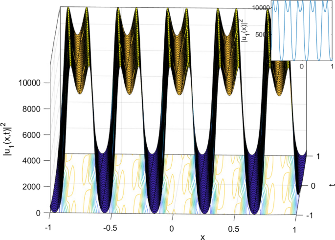
The graphics of Eq. (29) solution for \(\gamma _{1}=0.5\), \(r=-0.05\), \(\mu =-1.2\), \(\beta =0.04\), \(\gamma _{2}=2.5\), and \(\rho =1\)
$$\begin{aligned} u_{2}(x,t)= \frac{3\left( {{r}^{2}}-\mu \right) \left( 1-\sqrt{-2}\text {csch}\left( \sqrt{{{\gamma }_{1}}}\left( \frac{\left( -rt+x \right) \sqrt{-{{r}^{2}}+\mu }}{r\sqrt{2{{\gamma }_{1}}}}+\rho \right) \right) \right) }{2\beta }. \end{aligned}$$(30)Fig. 2 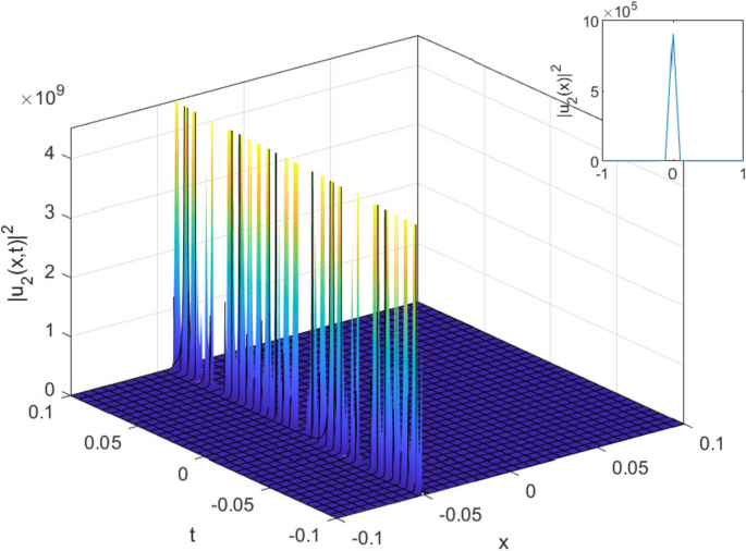
The graphics of Eq. (30) solution for \(\gamma _{1}=0.5\), \(r=0.05\), \(\mu =1.2\), \(\beta =0.04\), \(\gamma _{2}=-0.5\), and \(\rho =1\)
-
2.
When \(\gamma _{0} = 0\), \(\gamma _{1} > 0\), and \(\gamma _{2} =\pm 4 \beta _{1} \beta _{2}\), considering Eq. (11), so the solution of Eq. (2) is given by
$$\begin{aligned} \begin{aligned} u_{3}(x,t)=\frac{3\left( {{r}^{2}}-\mu \right) }{2\beta }\\ \, \, \, \, \, \, \, \, \, \, \, \, \, \, \, \, \, \, \, \, \, \, \, \, -\frac{12\sqrt{-2{{\beta }_{1}}{{\beta }_{2}}}\left( {{r}^{2}}-\mu \right) }{\beta \left( \left( 4{{\beta }_{1}}-4{{\beta }_{2}} \right) \text {cosh} \left( \sqrt{{{\gamma }_{1}}}\left( {{\chi }_{0}}+\frac{\left( -rt+x \right) \sqrt{-{{r}^{2}}+\mu }}{r\sqrt{2{{\gamma }_{1}}}} \right) \right) +\left( 4{{\beta }_{1}}+4{{\beta }_{2}} \right) \sinh \left( \sqrt{{{\gamma }_{1}}}\left( {{\chi }_{0}}+\frac{\left( -rt+x \right) \sqrt{-{{r}^{2}}+\mu }}{r\sqrt{2{{\gamma }_{1}}}} \right) \right) \right) }.\\ \end{aligned} \end{aligned}$$(31)Fig. 3 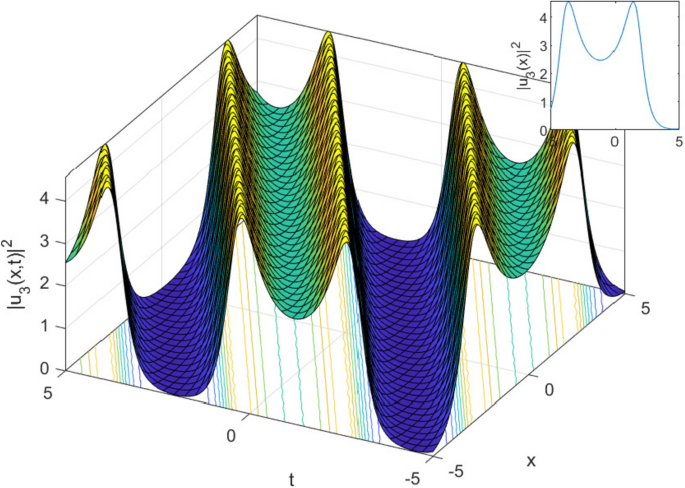
The graphics of Eq. (31) solution for \(\gamma _{1}=0.5\), \(r=1.75\), \(\mu =1.2\), \(\beta =4\), \(\eta _{0}=1\), \(\beta _{1} =2\) and \(\beta _{2} =3\)
-
3.
When \(\gamma _{0} = \frac{\gamma _{1}^2}{4 \gamma _{2}}\), \(\gamma _{1} < 0\), and \(\gamma _{2} > 0\), considering Eqs. (10), (11), (12), (13) and (14) respectively, so the solutions of Eq. (2) are given by
$$\begin{aligned} u_{4}(x,t)= \frac{3\left( {{r}^{2}}-\mu \right) }{2\beta }-\frac{3\left( {{r}^{2}}-\mu \right) \tanh \left( \frac{\sqrt{-{{\gamma }_{1}}}\left( \frac{\left( -rt+x \right) \sqrt{-{{r}^{2}}+\mu }}{r\sqrt{2{{\gamma }_{1}}}}+\rho \right) }{\sqrt{2}} \right) }{2\beta }. \end{aligned}$$(32)Fig. 4 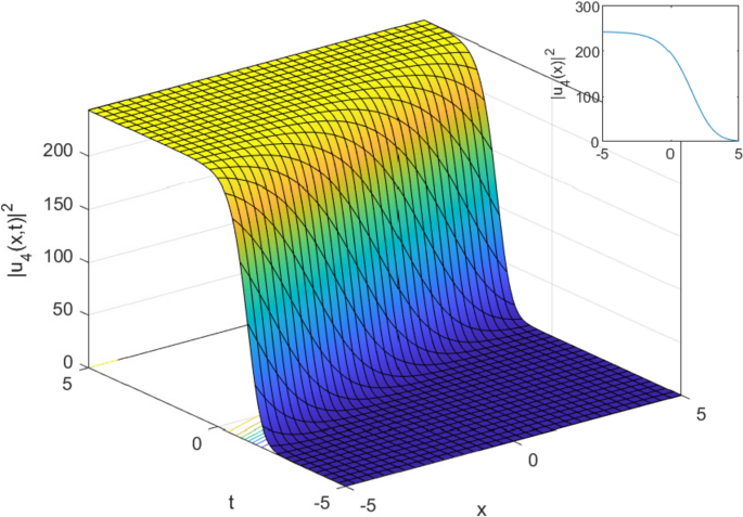
The graphics of Eq. (32) solution for \(\gamma _{1}=-0.2\), \(r=3\), \(\mu =1.2\), \(\beta =1.5\), \(\gamma _{2}=0.1\) and \(\rho =1\)
$$\begin{aligned} u_{5}(x,t)= \frac{3\left( {{r}^{2}}-\mu \right) }{2\beta }-\frac{3\left( {{r}^{2}}-\mu \right) \coth \left[ \frac{\sqrt{-{{\gamma }_{1}}}\left( \frac{\left( -rt+x \right) \sqrt{-{{r}^{2}}+\mu }}{r\sqrt{2{{\gamma }_{1}}}}+\rho \right) }{\sqrt{2}} \right] }{2\beta } \end{aligned}$$(33)Fig. 5 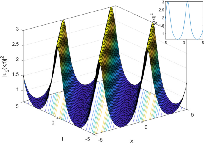
The graphics of (33) solution for \(\gamma _{1}=-0.5\), \(r=0.9\), \(\mu =2\), \(\beta =1.2\), \(\gamma _{2}=2\),, and \(\rho =1\)
$$\begin{aligned} \begin{aligned} u_{6}(x,t)= \frac{3\left( {{r}^{2}}-\mu \right) }{2\beta }\\ \, \, \, \, \, \, \, \, \, \, \, \, \, \, \, \, \, \, \, \, \, \, \, \, \, -\frac{3\left( {{r}^{2}}-\mu \right) \left( \text {i}\text {sech}\left( \sqrt{-2{{\gamma }_{1}}}\left( \frac{\left( -rt+x \right) \sqrt{-{{r}^{2}}+\mu }}{\sqrt{2}r\sqrt{{{\gamma }_{1}}}}+\rho \right) \right) +\tanh \left( \sqrt{-2{{\gamma }_{1}}}\left( \frac{\left( -rt+x \right) \sqrt{-{{r}^{2}}+\mu }}{\sqrt{2}r\sqrt{{{\gamma }_{1}}}}+\rho \right) \right) \right) }{2\beta }, \\ \end{aligned} \end{aligned}$$(34)$$\begin{aligned} \begin{aligned} u_{7}(x,t)= \frac{3\left( {{r}^{2}}-\mu \right) }{2\beta } \\ \, \, \, \, \, \, \, \, \, \, \, \, \, \, \, \, \, \, \, \, \, \, \, \, \, -\frac{3\left( {{r}^{2}}-\mu \right) \left( \coth \left( \frac{\sqrt{-{{\gamma }_{1}}}\left( \frac{\left( -rt+x \right) \sqrt{-{{r}^{2}}+\mu }}{\sqrt{2}r\sqrt{{{\gamma }_{1}}}}+\rho \right) }{2\sqrt{2}} \right) +\tanh \left( \frac{\sqrt{-{{\gamma }_{1}}}\left( \frac{\left( -rt+x \right) \sqrt{-{{r}^{2}}+\mu }}{\sqrt{2}r\sqrt{{{\gamma }_{1}}}}+\rho \right) }{2\sqrt{2}} \right) \right) }{4\beta },\\ \end{aligned} \end{aligned}$$(35)$$\begin{aligned} u_{8}(x,t)= \frac{3\left( {{r}^{2}}-\mu \right) }{2\beta }-\frac{3\left( {{r}^{2}}-\mu \right) \cosh \left( \sqrt{-2{{\gamma }_{1}}}\left( \frac{\left( -rt+x \right) \sqrt{-{{r}^{2}}+\mu }}{\sqrt{2}r\sqrt{{{\gamma }_{1}}}}+\rho \right) \right) }{2\beta \left( \text {i}+\sinh \left( \sqrt{-2\gamma 1}\left( \frac{\left( -rt+x \right) \sqrt{-{{r}^{2}}+\mu }}{\sqrt{2}r\sqrt{{{\gamma }_{1}}}}+\rho \right) \right) \right) }. \end{aligned}$$(36) -
4.
When \(\gamma _{0} = 0\), \(\gamma _{1} < 0\), and \(\gamma _{2} \ne 0\), considering Eqs. (15) and (16) respectively, so the solutions of Eq. (2) are given by
$$\begin{aligned} u_{9}(x,t)= \frac{3\left( {{r}^{2}}-\mu \right) }{2\beta }-\frac{3\left( {{r}^{2}}-\mu \right) \sec \left( \sqrt{-{{\gamma }_{1}}}\left( \frac{\left( -rt+x \right) \sqrt{-{{r}^{2}}+\mu }}{r\sqrt{2{{\gamma }_{1}}}}+\rho \right) \right) }{\sqrt{2}\beta }, \end{aligned}$$(37)$$\begin{aligned} u_{10}(x,t)= \frac{3\left( {{r}^{2}}-\mu \right) }{2\beta }-\frac{3\left( {{r}^{2}}-\mu \right) \csc \left( \sqrt{-{{\gamma }_{1}}}\left( \frac{\left( -rt+x \right) \sqrt{-{{r}^{2}}+\mu }}{r\sqrt{2{{\gamma }_{1}}}}+\rho \right) \right) }{\sqrt{2}\beta }. \end{aligned}$$(38) -
5.
When \(\gamma _{0}=\frac{\gamma _{1}^2}{4 \gamma _{2}}\), \(\gamma _{1}>0\), and \(\gamma _{2}> 0 \), with constants \(A_{1}^2- A_{2}^2>0\), considering Eqs. (17), (18), (19), (20), (21), and (22) respectively, so the solutions of Eq. (2) are given by
$$\begin{aligned} u_{11}(x,t)= \frac{3\left( {{r}^{2}}-\mu \right) }{2\beta }-\frac{3i\left( {{r}^{2}}-\mu \right) \tan \left( \frac{\sqrt{{{\gamma }_{1}}}\left( \frac{\left( -rt+x \right) \sqrt{-{{r}^{2}}+\mu }}{\sqrt{2}r\sqrt{{{\gamma }_{1}}}}+\rho \right) }{\sqrt{2}} \right) }{2\beta }, \end{aligned}$$(39)Fig. 6 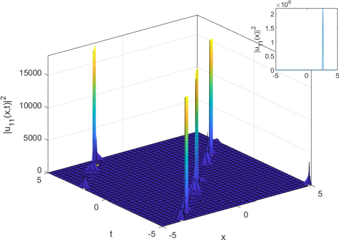
The graphics of (39) solution for \(\gamma _{1}=2\), \(r=1.05\), \(\mu =1.7\), \(\beta =2.3\), \(\gamma _{2}=0.6\) and \(\rho =1\)
$$\begin{aligned} u_{12}(x,t)= \frac{3\left( {{r}^{2}}-\mu \right) }{2\beta }-\frac{3\text {i}\left( {{r}^{2}}-\mu \right) \cot \left( \frac{\sqrt{{{\gamma }_{1}}}\left( \frac{\left( -rt+x \right) \sqrt{-{{r}^{2}}+\mu }}{\sqrt{2}r\sqrt{{{\gamma }_{1}}}}+\rho \right) }{\sqrt{2}} \right) }{2\beta } \end{aligned}$$(40)Fig. 7 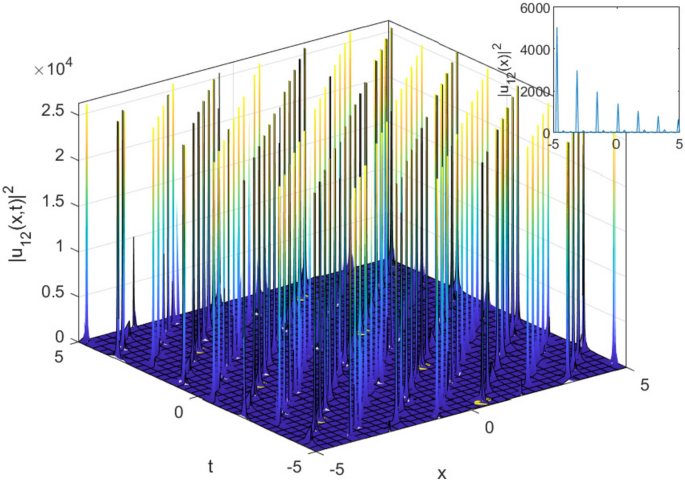
The graphics of (40) solution for \(\gamma _{1}=0.004\), \(r=0.1\), \(\mu =1.4\), \(\beta =1.25\), \(\gamma _{2}=2\) and \(\rho =1\)
$$\begin{aligned} \begin{aligned} u_{13}(x,t)=\frac{3\left( {{r}^{2}}-\mu \right) }{2\beta }\\ \, \, \, \, \, \, \, \, \, \, \, \, \, \, \, \, \, \, \, \, \, \, \, \, \,-\frac{3\text {i}\left( {{r}^{2}}-\mu \right) \left( \sec \left( \sqrt{2{{\gamma }_{1}}}\left( \frac{\left( -rt+x \right) \sqrt{-{{r}^{2}}+\mu }}{r\sqrt{2{{\gamma }_{1}}}}+\rho \right) \right) +\tan \left( \sqrt{2{{\gamma }_{1}}}\left( \frac{\left( -rt+x \right) \sqrt{-{{r}^{2}}+\mu }}{r\sqrt{2{{\gamma }_{1}}}}+\rho \right) \right) \right) }{2\beta },\\ \end{aligned} \end{aligned}$$(41)$$\begin{aligned} \begin{aligned} u_{14}(x,t)= \frac{3\left( {{r}^{2}}-\mu \right) }{2\beta } \\ \, \, \, \, \, \, \, \, \, \, \, \, \, \, \, \, \, \, \, \, \, \, \, \, \, -\frac{3\text {i}\left( {{r}^{2}}-\mu \right) \left( -\cot \left( \frac{\sqrt{{{\gamma }_{1}}}\left( \frac{\left( -rt+x \right) \sqrt{-{{r}^{2}}+\mu }}{\sqrt{2}r\sqrt{{{\gamma }_{1}}}}+\rho \right) }{2\sqrt{2}} \right) +\tan \left( \frac{\sqrt{{{\gamma }_{1}}}\left( \frac{\left( -rt+x \right) \sqrt{-{{r}^{2}}+\mu }}{\sqrt{2}r\sqrt{{{\gamma }_{1}}}}+\rho \right) }{2\sqrt{2}} \right) \right) }{4\beta }, \\ \end{aligned} \end{aligned}$$(42)$$\begin{aligned} \begin{aligned} u_{15}(x,t)=\frac{3\left( {{r}^{2}}-\mu \right) }{2\beta }\\ \, \, \, \, \, \, \, \, \, \, \, \, \, \, \, \, \, \, \, \, \, \, \, \, \,-\frac{3\text {i}\left( {{r}^{2}}-\mu \right) \left( \sqrt{{{A}_{1}}^{2}-{{A}_{2}}^{2}}-{{A}_{1}}\cos \left( \sqrt{2{{\gamma }_{1}}}\left( \frac{\left( -rt+x \right) \sqrt{-{{r}^{2}}+\mu }}{\sqrt{2}r\sqrt{{{\gamma }_{1}}}}+\rho \right) \right) \right) }{2\beta \left( {{A}_{2}}+{{A}_{1}}\sin \left( \sqrt{2{{\gamma }_{1}}}\left( \frac{\left( -rt+x \right) \sqrt{-{{r}^{2}}+\mu }}{\sqrt{2}r\sqrt{{{\gamma }_{1}}}}+\rho \right) \right) \right) }, \\ \end{aligned} \end{aligned}$$(43)Fig. 8 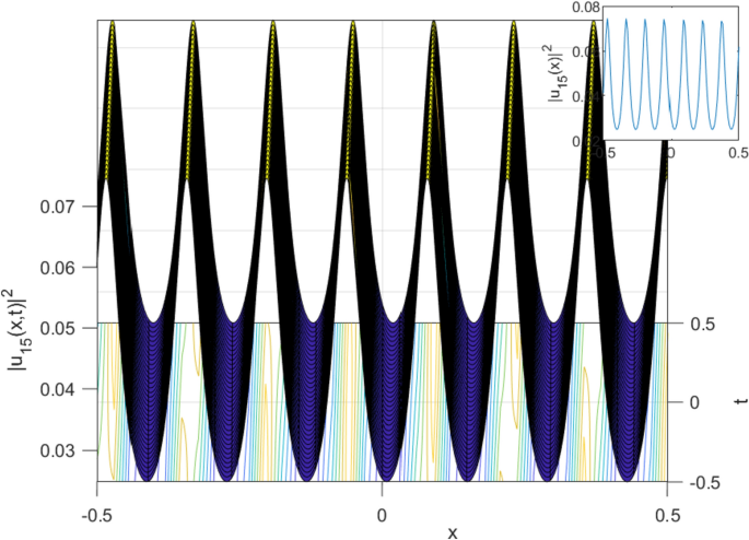
The graphics of (43) solution for \(\gamma _{1}=0.5\), \(r=0.01\), \(\mu =0.2\), \(\beta =3\), \(\gamma _{2}=0.3\), \(A_{1}=0.1\), \(A_{2}=0.2\) and \(\rho =1\)
$$\begin{aligned} u_{16}(x,t)= \frac{3\left( {{r}^{2}}-\mu \right) }{2\beta }-\frac{3\text {i}\left( {{r}^{2}}-\mu \right) \cos \left( \sqrt{2{{\gamma }_{1}}}\left( \frac{\left( -rt+x \right) \sqrt{-{{r}^{2}}+\mu }}{r\sqrt{2{{\gamma }_{1}}}}+\rho \right) \right) }{2\beta \left( 1+\sin \left( \sqrt{2{{\gamma }_{1}}}\left( \frac{\left( -rt+x \right) \sqrt{-{{r}^{2}}+\mu }}{r\sqrt{2{{\gamma }_{1}}}}+\rho \right) \right) \right) }. \end{aligned}$$(44)Fig. 9 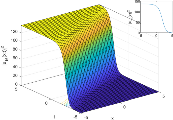
The graphics of (44) solution for \(\gamma _{1}=0.03\), \(r=2\), \(\mu =0.1\), \(\beta =1\), \(\gamma _{2}=0.01\) and \(\rho =1\)
-
6.
When \(\gamma _{0}=0\), \(\gamma _{1}>0\), considering Eq. (23), and Eq. (24) respectively, so the solutions of Eq. (2) are given by
$$\begin{aligned} u_{17}(x,t)= \frac{3\left( {{r}^{2}}-\mu \right) }{2\beta }-\frac{6\sqrt{2}{{\text {e}}^{\sqrt{{{\gamma }_{1}}}\left( \frac{\left( -rt+x \right) \sqrt{-{{r}^{2}}+\mu }}{\sqrt{2}r\sqrt{{{\gamma }_{1}}}}+\rho \right) }}\sqrt{-{{\gamma }_{1}}{{\gamma }_{2}}}\left( {{r}^{2}}-\mu \right) }{\beta \left( {{\text {e}}^{2\sqrt{{{\gamma }_{1}}}\left( \frac{\left( -rt+x \right) \sqrt{-{{r}^{2}}+\mu }}{\sqrt{2}r\sqrt{{{\gamma }_{1}}}}+\rho \right) }}-4{{\gamma }_{1}}{{\gamma }_{2}} \right) }, \end{aligned}$$(45)$$\begin{aligned} u_{18}(x,t)=\frac{3\left( {{r}^{2}}-\mu \right) }{2\beta }-\frac{6\sqrt{2}{{\text {e}}^{\sqrt{{{\gamma }_{1}}}\left( \frac{\left( -rt+x \right) \sqrt{-{{r}^{2}}+\mu }}{\sqrt{2}r\sqrt{{{\gamma }_{1}}}}+\rho \right) }}\sqrt{-{{\gamma }_{1}}{{\gamma }_{2}}}\left( {{r}^{2}}-\mu \right) }{\beta \left( 1-4{{\text {e}}^{2\sqrt{{{\gamma }_{1}}}\left( \frac{\left( -rt+x \right) \sqrt{-{{r}^{2}}+\mu }}{\sqrt{2}r\sqrt{{{\gamma }_{1}}}}+\rho \right) }}{{\gamma }_{1}}{{\gamma }_{2}} \right) }. \end{aligned}$$(46)


4 Conclusions
This paper introduces a novel approach using MSSEM to analyze various solutions of the generalized Pochhammer Chree equation that describes the propagation of longitudinal deformation waves in an elastic rod. The generalized Pochhammer Chree equation is a fundamental equation in the field of solid mechanics. It characterizes the behavior of an elastic rod subjected to longitudinal forces or deformations. It takes into account the material properties of the rod, such as its elasticity and density, as well as the wave propagation characteristics, such as the wave speed. Through the solution of the equation, we gain the capability to analyze the behavior of the rod under diverse loading conditions. This enables a comprehensive study of the propagation of deformation waves along the length of the rod. By applying mathematical methods to address the equation, we unlock insights into how the rod responds to varying external forces or conditions, allowing for a detailed examination of the dynamic processes involved in the transmission of deformation waves. This analytical approach provides a valuable tool for understanding the intricate mechanics governing the rod’s response to different stimuli and contributes to a deeper comprehension of wave propagation phenomena in the context of structural materials. This equation is widely used in various fields, including structural engineering, mechanical engineering, and materials science, to understand and design structures and systems involving elastic rods. To provide a physical interpretation of the solutions and better understand this situation, we present them graphically in Figs. 1, 2, 3, 4, 5, 6, 7, 8, 9. Figures 1, 2, 3, 4, 5, 6, 7, 8, 9 shows how the settings have an influence. In addition, it can be interpreted from the figures that each solution is different and the solutions it belongs to have different structures.Muhammad et al. (yyy) Apart from this, it can be seen that the solutions found are different from studies such as solitary solutions (Yokus et al. 2022), periodic wave solutions (Parand and Rad 2010; Jaradat et al. 2022; Ali et al. 2020) and soliton solutions (Hussain et al. 2023). These figures visually depict the behavior and characteristics of the solutions, allowing for a clearer understanding of the propagation of longitudinal deformation waves in the elastic rod. Consequently, the solutions obtained are in the form of bright solutions for Eq. (29) as presented in Fig. 1, singular solutions for Eqs. (29), and (33) as shown in Figs. 2 and 5, trigonometric solutions for Eqs. (31), (43) and (44) as seen in Figs. 3, 8 and 8 , dark solutions for Eq. (32) as presented in Fig. 4, and periodic solutions for Eq. (39) and Eq. (40) as presented in Figs. 6 and Fig. 7. This diverse set of solution types provides valuable insights into the complex dynamics and phenomena associated with the propagation of longitudinal deformation waves in elastic rods. It showcases the effectiveness of these methods in capturing the rich complexity of nonlinear partial differential equations and their applications in fields such as physics, engineering, and applied mathematics.
References
Ahmed, H.M., El-Sheikh, M.M.A., Arnous, A.H., Rabie, W.B.: Construction of the soliton solutions for the Manakov system by extended simplest equation method. Int. J. Appl. Comput. Math. 7, 1–19 (2021)
Akinyemi, L., Akpan, U., Veeresha, P., Rezazadeh, H., İnç, M.: Computational techniques to study the dynamics of generalized unstable nonlinear Schrödinger equation. J. Ocean Eng. Sci. (2022)
Akinyemi, L., Rezazadeh, H., Shi, Q.H., Inc, M., Khater, M.M., Ahmad, H., Akbar, M.A.: New optical solitons of perturbed nonlinear Schrödinger-Hirota equation with spatio-temporal dispersion. Res. Phys. 29, 104656 (2021)
Akinyemi, L.: Two improved techniques for the perturbed nonlinear Biswas-Milovic equation and its optical solitons. Optik 243, 167477 (2021)
Al-Amr, M.O.: Exact solutions of the generalized (2+ 1)-dimensional nonlinear evolution equations via the modified simple equation method. Comput. Math. Appl. 69(5), 390–397 (2015)
Al-Bugami, A. M., Abdou, M. A., Mahdy, A.: Sixth-Kind Chebyshev and Bernoulli polynomial numerical methods for solving nonlinear mixed partial integrodifferential equations with continuous Kernels. J. Funcct. Spaces 2023 1–14 (2023)
Ali, K. K., Tarla, S., Yusuf, A., Yilmazer, R.: Closed form wave profiles of the coupled-Higgs equation via the \(\phi ^6\)-model expansion method. Int. J. Mod. Phys. B 37, 2350070 (2022)
Ali, K., Yusuf, A., Ma, W. X.: Dynamical rational solutions and their interaction phenomena for an extended nonlinear equation. Commun. Theor. Phys. 75(3), 035001 (2023)
Ali, A., Seadawy, A.R., Baleanu, D.: Propagation of harmonic waves in a cylindrical rod via generalized Pochhammer-Chree dynamical wave equation. Res. Phys. 17, 103039 (2020)
Ali, K.K., Golmankhaneh, A.K., Yilmazer, R.: Battery discharging model on fractal time sets. Int. J. Nonlinear Sci. Numer. Simul. 24(1), 71–80 (2023)
Ali, K.K., Tarla, S., Ali, M.R., Yusuf, A., Yilmazer, R.: Consistent solitons in the plasma and optical fiber for complex Hirota-dynamical model. Res. Phys. 47, 106393 (2023)
Ali, K.K., Tarla, S., Ali, M.R., Yusuf, A.: Modulation instability analysis and optical solutions of an extended (2+ 1)-dimensional perturbed nonlinear Schrödinger equation. Res. Phys. 45, 106255 (2023)
Alia, K., Rehmanb, H. U., Habibb, A., Awanc, A. U.: Study of Langmuir waves for Zakharov equation using Sardar sub-equation method. Int. J. Nonlinear Anal. Appl. 1, 12 (1402)
Anaç, H.: The novel investigation to Fornberg-Whitham equation via fractional natural transform decomposition method (2023)
Asif, M., Nawaz, R., Nuruddeen, R.I.: Dispersion of an inhomogeneous sandwich plate having imperfect interfaces and supported by the Pasternak foundation. Smart Mater. Struct. 32(12), 125002 (2023)
Asif, M., Nawaz, R., Nuruddeen, R.I.: Dispersion of elastic waves in the three-layered inhomogeneous sandwich plate embedded in the Winkler foundations. Sci. Prog. 106(2), 00368504231172585 (2023)
Asjad, M.I., Munawar, N., Muhammad, T., Hamoud, A.A., Emadifar, H., Hamasalh, F.K., Khademi, M.: Traveling wave solutions to the Boussinesq equation via Sardar sub-equation technique. AIMS Math. 7(6), 11134–11149 (2022)
Batool, N., Masood, W., Siddiq, M., Alrowaily, A.W., Ismaeel, S.M., El-Tantawy, S.A.: Hirota bilinear method and multi-soliton interaction of electrostatic waves driven by cubic nonlinearity in pair-ion-electron plasmas. Phys. Fluids 35(3), 033109 (2023)
Bogolubsky, I.L.: Some examples of inelastic soliton interaction. Comput. Phys. Commun. 13(3), 149–155 (1977)
Cinar, M., Secer, A., Ozisik, M., Bayram, M.: Derivation of optical solitons of dimensionless Fokas-Lenells equation with perturbation term using Sardar sub-equation method. Opt. Quant. Electron. 54(7), 402 (2022)
Cinar, M., Secer, A., Ozisik, M., Bayram, M.: Optical soliton solutions of (1+ 1)-and (2+ 1)-dimensional generalized Sasa-Satsuma equations using new Kudryashov method. Int. J. Geom. Methods Mod. Phys. 20(2), 2350034 (2023)
Clarkson, P.A., LeVeque, R.J., Saxton, R.: Solitary-wave interactions in elastic rods. Stud. Appl. Math. 75(2), 95–121 (1986)
El Sheikh, M.M.A., Ahmed, H.M., Arnous, A.H., Rabie, W.B., Biswas, A., Khan, S., Alshomrani, A.S.: Optical solitons with differential group delay for coupled Kundu-Eckhaus equation using extended simplest equation approach. Optik 208, 164051 (2020)
El-Ganaini, S.I.A.: Travelling wave solutions to the generalized Pochhammer-Chree (PC) equations using the first integral method. Math. Proble. Eng. 2011, 1–13 (2011)
El-Ganaini, S., Kumar, S., Niwas, M.: Construction of multiple new analytical soliton solutions and various dynamical behaviors to the nonlinear convection-diffusion-reaction equation with power-law nonlinearity and density-dependent diffusion via Lie symmetry approach together with a couple of integration approaches. J. Ocean Eng. Sci. 8(3), 226–237 (2023)
Esen, H., Secer, A., Ozisik, M., Bayram, M.: Obtaining soliton solutions of the nonlinear (4+ 1)-dimensional Boiti-Leon-Manna-Pempinelli equation via two analytical techniques. Int. J. Mod. Phys. B, 38(1) 2450010 (2023)
Faisal, K., Abbagari, S., Pashrashid, A., Houwe, A., Yao, S. W., & Ahmad, H.: Pure-cubic optical solitons to the Schrödinger equation with three forms of nonlinearities by Sardar subequation method. Res. Phys. 48 106412 (2023)
Günerhan, H.: Exact traveling wave solutions of the Gardner equation by the improved tan\({\Theta }\)-expansion method and the wave ansatz method. Math. Prob. Eng. 2020(13), 9 (2020)
Günerhan, H., Khodadad, F.S., Rezazadeh, H., Khater, Mostafa M. A.: Exact optical solutions of the (2+1) dimensions Kundu-Mukherjee-Naskar model via the new extended direct algebraic method. Mod. Phys. Lett. B 34(22), 2050225 (2020)
Hassan, S.M., Altwaty, A.A.: Optical solitons of the extended Gerdjikov-Ivanov equation in DWDM system by extended simplest equation method. Appl. Math. 14(5), 901–907 (2020)
Hussain, A., Usman, M., Zaman, F. D., Eldin, S. M.: Double reductions and traveling wave structures of the generalized Pochhammer-Chree equation. Part. Differ. Equs. Appl. Math. 7, 100521 (2023)
Isah, M. A.: The novel optical solitons with complex Ginzburg-Landau equation for parabolic nonlinear form using the \(\phi ^6\)-model expansion approach. Math. Eng. Sci. Aerosp. (MESA), 14(1) 205–225 (2023)
Isah, M.A., Yokus, A.: Application of the newly \(\phi ^6\)-model expansion approach to the nonlinear reaction-diffusion equation. Open J. Math. Sci 6, 269–280 (2022)
Isah, M.A., YOKUS, A.: The investigation of several soliton solutions to the complex Ginzburg-Landau model with Kerr law nonlinearity. Math. Model. Numer. Simul. Appl. 2(3), 147–163 (2022)
Ismael, H. F., Younas, U., Sulaiman, T. A., Nasreen, N., Shah, N. A., Ali, M. R.: Non classical interaction aspects to a nonlinear physical model. Res. Phys. 49, 106520 (2023)
Ismael, H.F., Sulaiman, T.A.: On the dynamics of the nonautonomous multi-soliton, multi-lump waves and their collision phenomena to a (3+ 1)-dimensional nonlinear model. Chaos Solit. Fract. 169, 113213 (2023)
Ismael, H.F., Hafidzuddin, M.E.H., Murad, M.A.S., Arifin, N.M., Bulut, H.: Analysis of Tangent Hyperbolic over a Vertical Porous Sheet of Carreau Fluid and Heat Transfer. CFD Lett. 15(5), 86–96 (2023)
Ismael, H.F., Baskonus, H.M., Bulut, H., Gao, W.: Instability modulation and novel optical soliton solutions to the Gerdjikov-Ivanov equation with M-fractional. Opt. Quant. Electron. 55(4), 303 (2023)
Jaradat, I., Alquran, M., Qureshi, S., Sulaiman, T.A., Yusuf, A.: Convex-rogue, half-kink, cusp-soliton and other bidirectional wave-solutions to the generalized Pochhammer-Chree equation. Phys. Scr. 97(5), 055203 (2022)
Kamal Ali, K., Khalili Golmankhaneh, A., Yilmazer, R., Ashqi Abdullah, M.: Solving fractal differential equations via fractal Laplace transforms. J. Appl. Anal. 28(2), 237–250 (2022)
Li, J., Zhang, L.: Bifurcations of traveling wave solutions in generalized Pochhammer-Chree equation. Chaos Solit. Fract. 14(4), 581–593 (2002)
Liu, Y.: Existence and blow up of solutions of a nonlinear Pochhammer-Chree equation. Indiana Univ. Math. J. 45(3), 797–816 (1996)
Mahdy, A. M. S.: A numerical method for solving the nonlinear equations of Emden-Fowler models. J. Ocean Eng. Sci. (2022)
Mahdy, A. M.: Stability, existence, and uniqueness for solving fractional glioblastoma multiforme using a Caputo-Fabrizio derivative. Math. Methods Appl. Sci. 1–18 (2023)
Mahdy, A.M.S., Mohamed, D.S.: Approximate solution of Cauchy integral equations by using Lucas polynomials. Comput. Appl. Math. 41(8), 403 (2022)
Mahdy, A.M., Babatin, M.M., Khader, M.M.: Numerical treatment for processing the effect of convective thermal condition and Joule heating on Casson fluid flow past a stretching sheet. Int. J. Mod. Phys. C 33(08), 2250108 (2022)
Mahdy, A.M., Lotfy, K., El-Bary, A.A.: Use of optimal control in studying the dynamical behaviors of fractional financial awareness models. Soft. Comput. 26(7), 3401–3409 (2022)
Mahdy, A.M., Lotfy, K., El-Bary, A., Atef, H.M., Allan, M.: Influence of variable thermal conductivity on wave propagation for a ramp-type heating semiconductor magneto-rotator hydrostatic stresses medium during photo-excited microtemperature processes. Waves Rand. Complex Media 33(3), 657–679 (2023)
Mahdy, A.M., Nagdy, A.S., Hashem, K.M., Mohamed, D.S.: A computational technique for solving three-dimensional mixed Volterra-Fredholm integral equations. Fract. Fraction. 7(2), 196 (2023)
Malik, S., Hashemi, M.S., Kumar, S., Rezazadeh, H., Mahmoud, W., Osman, M.S.: Application of new Kudryashov method to various nonlinear partial differential equations. Opt. Quant. Electron. 55(1), 8 (2023)
Mandal, U.K., Malik, S., Kumar, S., Das, A.: A generalized (2+ 1)-dimensional Hirota bilinear equation: integrability, solitons and invariant solutions. Nonlinear Dyn. 111(5), 4593–4611 (2023)
Mohebbi, A.: Solitary wave solutions of the nonlinear generalized Pochhammer-Chree and regularized long wave equations. Nonlinear Dyn. 70, 2463–2474 (2012)
Mubaraki, A.M., Nuruddeen, R.I., Gómez-Aguilar, J.F.: Modeling the dispersion of waves on a loaded bi-elastic cylindrical tube with variable material constituents. Res. Phys. 53, 106927 (2023)
Mubaraki, A.M., Nuruddeen, R.I., Ali, K.K., Gómez-Aguilar, J.F.: Additional solitonic and other analytical solutions for the higher-order Boussinesq-Burgers equation. Opt. Quant. Electron. 56(2), 165 (2024)
Muhammad, T., Hamoud, A. A., Emadifar, H., Hamasalh, F. K., Azizi, H., Khademi, M.: Traveling wave solutions to the Boussinesq equation via Sardar sub-equation technique. AIMS Mathematics, 7(6), 11134-11149 (2022)
Murad, M.A.S., Hamasalh, F.K., Ismael, H.F.: Various optical solutions for time-fractional Fokas system arises in monomode optical fibers. Opt. Quant. Electron. 55(4), 300 (2023)
Murad, M.A.S., Hamasalh, F.K., Ismael, H.F.: Optical soliton solutions for time-fractional Fokas system in optical fiber by new Kudryashov approach. Optik 280, 170784 (2023)
Onder, I., Secer, A., Ozisik, M., Bayram, M.: Investigation of optical soliton solutions for the perturbed Gerdjikov-Ivanov equation with full-nonlinearity. Heliyon, 9(2) 13519 (2023)
Pandir, Y., Akturk, T., Gurefe, Y., Juya, H.: The modified exponential function method for beta time fractional Biswas-Arshed equation. Adv. Math. Phys. 2023 1091355 (2023)
Parand, K., Rad, J.A.: Some solitary wave solutions of generalized Pochhammer-Chree equation via Exp-function method. Int. J. Math. Comput. Sci. 4(7), 991–996 (2010)
Parand, K., Rad, J.A.: Some solitary wave solutions of generalized Pochhammer-Chree equation via Exp-function method. Int. J. Math. Comput. Sci. 4(7), 991–996 (2010)
Rehman, H. U., Inc, M., Asjad, M. I., Habib, A., Munir, Q.: New soliton solutions for the space-time fractional modified third order Korteweg-de Vries equation. J. Ocean Eng. Sci. (2022)
Rehman, H.U., Iqbal, I., Subhi Aiadi, S., Mlaiki, N., Saleem, M.S.: Soliton solutions of Klein-Fock-Gordon equation using Sardar subequation method. Mathematics 10(18), 3377 (2022)
Sadaf, M., Akram, G., Mariyam, H.: Abundant solitary wave solutions of Gardner’s equation using new \(\phi ^6\)-model expansion method. Alex. Eng. J. 61(7), 5253–5267 (2022)
Seadawy, A.R., Rizvi, S.T.R., Ahmad, S., Younis, M., Baleanu, D.: Lump, lump-one stripe, multiwave and breather solutions for the Hunter-Saxton equation. Open Phys. 19(1), 1–10 (2021)
Shawagfeh, N., Kaya, D.: Series solution to the Pochhammer-Chreeequation and comparison with exact solutions. Comput. Math. Appl. 47(12), 1915–1920 (2004)
Triki, H., Benlalli, A., Wazwaz, A.M.: Exact solutions of the generalized Pochhammer-Chree equation with sixth-order dispersion. Rom. J. Phys. 60, 935–951 (2015)
Ullah, M.S., Seadawy, A.R., Ali, M.Z.: Optical soliton solutions to the Fokas-Lenells model applying the \(\phi ^6\)-model expansion approach. Opt. Quant. Electron. 55(6), 495 (2023)
Ullah, N., Asjad, M.I., Hussanan, A., Akgül, A., Alharbi, W.R., Algarni, H., Yahia, I.S.: Novel waves structures for two nonlinear partial differential equations arising in the nonlinear optics via Sardar-subequation method. Alex. Eng. J. 71, 105–113 (2023)
Wazwaz, A.M.: The tanh-coth and the sine-cosine methods for kinks, solitons, and periodic solutions for the Pochhammer-Chree equations. Appl. Math. Comput. 195(1), 24–33 (2008)
Weiguo, Z., Wenxiu, M.: Explicit solitary-wave solutions to generalized Pochhammer-Chree equations. Appl. Math. Mech. 20(6), 625–632 (1999)
Yao, S.W., Shahzad, T., Ahmed, M.O., Baber, M.Z., Iqbal, M.S., Inc, M.: Extraction of soliton solutions for the time-space fractional order nonclassical Sobolev-type equation with unique physical problems. Res. Phys. 45, 106256 (2023)
Yao, S.W., Baber, M.Z., Inc, M., Iqbal, M.S., Jawaz, M., Akhtar, M.Z.: Investigation of nonlinear problems governed by stochastic phi-4 type equations in nuclear and particle physics. Res. Phys. 46, 106295 (2023)
Yokus, A., Isah, M.A.: Stability analysis and solutions of (2+ 1)-Kadomtsev-Petviashvili equation by homoclinic technique based on Hirota bilinear form. Nonlinear Dyn. 109(4), 3029–3040 (2022)
Yokus, A., Isah, M.A.: Dynamical behaviors of different wave structures to the Korteweg-de Vries equation with the Hirota bilinear technique, p. 128819. Statistical Mechanics and its Applications, Physica A (2023)
Yokus, A., Ali, K.K., Yılmazer, R., Bulut, H.: On exact solutions of the generalized Pochhammer-Chree equation. Comput. Methods Differ. Equs. 10(3), 746–754 (2022)
Yusuf, A., Alshomrani, A.S., Sulaiman, T.A., Isah, I., Baleanu, D.: Extended classical optical solitons to a nonlinear Schrodinger equation expressing the resonant nonlinear light propagation through isolated flaws in optical waveguides. Opt. Quant. Electron. 54(12), 1–13 (2022)
Zayed, E. M., El-Ganaini, S.: Comment on the article published in Math Meth Appl Sci. 2021; 44: 2682-2691. Math. Methods Appl. Sci, 47(1), 562–564 (2024)
Zayed, E.M., Shohib, R.M.: Optical solitons and other solutions to Biswas-Arshed equation using the extended simplest equation method. Optik 185, 626–635 (2019)
Zhang, W.L.: Solitary wave solutions and kink wave solutions for a generalized PC equation. Acta Math. Appl. Sinica 21, 125–134 (2005)
Zhang, W., Zhao, Y., Liu, G., Ning, T.: Periodic wave solutions for pochhammer-chree equation with five order nonlinear term and their relationship with solitary wave solutions. Int. J. Mod. Phys. B 24(19), 3769–3783 (2010)
Zhu, W. H., Pashrashid, A., Adel, W., GüNerhan, H., Nisar, K.S. Saleel A. Inc, M., Rezazadeh, H.: Dynamical behaviour of the foam drainage equation. Res. Phys. 30, 104844 (2021)
Zuo, J.M.: Application of the extended \(\frac{G^{\prime }}{G}\)-expansion method to solve the Pochhammer-Chree equations. Appl. Math. Comput. 217(1), 376–383 (2010)
Funding
Open access funding provided by the Scientific and Technological Research Council of Türkiye (TÜBİTAK). The authors have not disclosed any funding.
Author information
Authors and Affiliations
Corresponding author
Ethics declarations
Conflict of interest
The authors have not disclosed any competing interests.
Rights and permissions
Open Access This article is licensed under a Creative Commons Attribution 4.0 International License, which permits use, sharing, adaptation, distribution and reproduction in any medium or format, as long as you give appropriate credit to the original author(s) and the source, provide a link to the Creative Commons licence, and indicate if changes were made. The images or other third party material in this article are included in the article's Creative Commons licence, unless indicated otherwise in a credit line to the material. If material is not included in the article's Creative Commons licence and your intended use is not permitted by statutory regulation or exceeds the permitted use, you will need to obtain permission directly from the copyright holder. To view a copy of this licence, visit http://creativecommons.org/licenses/by/4.0/.
About this article

Cite this article
Tarla, S., Ali, K.K. & Günerhan, H. Optical soliton solutions of generalized Pochammer Chree equation. Opt Quant Electron 56, 899 (2024). https://doi.org/10.1007/s11082-024-06711-1
Received:
Accepted:
Published:
DOI: https://doi.org/10.1007/s11082-024-06711-1