The application of the bilinear foil model to three-pad foil air bearings in rotordynamic analysis including reduced order modelling

Abstract

Foil air bearings (FABs) are the mainstay of oil-free turbomachinery technology which is undergoing rapid expansion. A rotor system using such bearings is a nonlinear multi-domain dynamical system comprising the rotor, the air films and the foil structures. Multi-pad (segmented) FABs offer opportunity for enhanced stability performance but are naturally more computationally challenging than single (360°) pad FABs. Their analysis has been limited to a simple model that ignores the detachment of the top foil from the underlying foil. Although a correction can be applied for the rotor vibration, the actual top foil deflection cannot be predicted. Additionally, reduced order modelling techniques have so far not been applied to such bearings. This paper presents the nonlinear and linearised dynamic analyses of three-pad FAB rotor systems considering foil detachment and using both Galerkin Reduction (GR) and Finite Difference (FD) to model the air film. Various models for the force distribution on the top foil are considered for use within a bilinear foil model, focusing on the ability to achieve numerical convergence. GR halved the computation time for a waterfall graph, without compromising the accuracy of the prediction of the nonlinear response. The results are validated against results from the literature.

1 Introduction

The environmental and technological advantages of replacing oil or grease-lubricated bearings with oil-free alternatives have motivated research into foil air bearing (FAB) technology [1,2,3,4]. The lubrication in FABs is provided by the air film between the journal and a compliant foil structure that comprises a top foil (forming the bearing surface) and an underlying supporting spring (typically in the form of a corrugated foil referred to as “bump foil”). The FAB is self-acting i.e. the air film is pressurised by the hydrodynamic action induced by the rotation of the journal relative to the top foil. Despite having numerous benefits over conventional bearings [1,2,3], a significant drawback that has limited the usage of the FAB is the complexity of its mathematical model in comparison with conventional journal bearings, presenting a greater challenge to predict nonlinear phenomena. Experimental results reveal non-linear responses with sub-synchronous vibrations that are not predicted by conventional theoretical models based on rotordynamic coefficients [5].

The prediction of such phenomena requires due consideration of the nonlinear multi-domain dynamical system that comprises the coupling between the rotor, the air films and the foil structures where each is governed by a set of time-based differential equations [6, 7]. The nonlinear time domain solution approach used in the present paper is based on Bonello and Pham's [8, 9] simultaneous solution of all state variables in time, which has also been followed by other researchers e.g. [6, 10]. This ensures that the multi-domain system remains fully coupled by allowing for the construction of a system of ordinary differential equations (ODEs) that can solve the compressible Reynolds Equation (governing the air films) as well as other state variables at each time step. The approach was further developed in [11] for linearized rotordynamic analysis, wherein eigenvalue analysis of the Jacobian of the fully coupled dynamical system system (evaluated at the static equilibrium condition of the nonlinear system) enabled the rapid prediction of the onset of instability speed (OIS) and a full modal analysis (expressed in a Campbell diagram). Such an approach was later used in [7, 12] and by other researchers in [12, 13]. As noted in [12] and demonstrated in [14], Jacobian-based linearization is superior to the traditional linearization approach based on linear force coefficients since the latter is unable to detect predicted instabilities that originate from the foil domain.

A foil air bearing (FAB) can be either single (360°) pad, or multi-pad (segmented). Figure 1b illustrates the latter type of bearing with three pads. Such an industry-designed bearing has been used in experimental and theoretical work by Larsen and co-authors [6, 13, 15,16,17,18,19] and in theoretical work by other authors [11, 14] who correlated their work with those of Larsen et al. The present paper will focus on three-pad FABs. As shown in Fig. 1b, each pad is free at the trailing edge (TE) and clamped at the leading edge (LE), facilitating an inlet slope at the LE which is found to influence static and dynamic results, particularly improving stability characteristics [6, 15, 16].

Fig. 1

Rotor-FAB system: a generic rotor system mounted on two FABs; b three pad bearing $\gamma$ (A or B)

In all the previous studies [6, 11, 13, 16] involving fully coupled (simultaneous) solution of rotor systems with three-pad FABs, the foil pad (comprising bump foil and top foil) has been modelled using a Simple Elastic Foundation model (SEFM) for the bump foil (top foil ignored [6, 11, 16]) or a variation thereof that additionally included the top foil as a non-detachable structure [13]. The classic SEFM is a popular choice because of its simplicity and computational efficiency, but it is subject to a number of assumptions and limitations:

• SEFM assumes that the foil stiffness is linear and ignores the stiffening effect generated by friction forces in the sliding contact points;

• it assumes a continuous distribution of compliance and damping wherein the foil deformation at any given point is dependent only on the pressure at that point;

• it ignores top foil sagging between bumps (deflection is based only on the bump foil);

• the SEFM cannot model the detachment of the top foil from the bump foil, which happens in air film regions that are below atmospheric pressure.

To compensate for this latter limitation, the Gümbel condition is applied wherein sub-atmospheric pressures are truncated when integrating for the air film forces on the journal [6, 11, 16]. This is based on the assumption that sub-atmospheric pressures will revert to atmospheric once the detached part of the top foil reaches an equilibrium position. This correction is only intended for the prediction of rotor vibration, and can be very effective in this regard when the foil pads have a clamped leading edge and free trailing edge (as with the three-pad bearing shown in Fig. 1b, which was considered in [6, 11, 16]). However, the Gümbel correction does not do anything to the foil deflection. As a consequence, simulations of foil deflection based on SEFM are not realistic in two principal ways:

• (a) they cannot simulate the detachment of the top foil (which is considered stuck to the bump foil);

• (b) the deflection at the free end of each pad is zero at all times (due to the second assumption listed above, since the pressure at the ends of a pad is atmospheric). It is noted that combining a classic SEFM for the bump foil with a non-detachable structural model for the top foil may result in a non-zero deflection at a free end (e.g. Figure 7 of [13]). However, even in such a case the pad deflection profile is still seen to be changing course and rapidly diminishing from a local maximum magnitude as it approaches the free end (due to the dominant influence of the SEFM).

This lack of a realistic representation of the foil deflection is naturally exacerbated with multi-pad bearings, which have openings to atmosphere at multiple angular locations (Fig. 1b). This means that the true distribution of the thickness of the air film cannot be predicted. It is therefore desirable to directly model the detachment of the top foil from the bump foil in multi-pad bearings using a bilinear foil model as done for single pad bearings in [20,21,22].

Multi-pad bearing systems are computationally intensive due to the need to consider the compressible Reynolds Equation (RE) for the air film of each pad within the solution process of the fully coupled multi-domain system. Up to now, the RE in three-pad FABs has been modelled through spatial discretization methods like Finite Element (FE) or Finite Difference (FD)/Finite Volume (FV). FE/FV involves element-based discretization of the RE and has been used in [6, 12, 13]. Element-based discretization usually needs a matrix assembly process to convert the RE from a partial differential equation (PDE) into a set of ordinary differential equations (ODEs), which can be time consuming knowing that it needs to be repeated at the beginning of each time-integration step. In another discretization approach, FD is used in [11, 20], which does not need any assembly process or interpolation of the field variable to derive the system of ODEs. In both FE [6, 23] and FD [9, 11, 16, 20, 24, 25] approaches, discretization is done spatially on a grid of nodes and the number of ODEs is the same as number of nodes, which can get very large in multi-pad FAB rotor systems. This problem can be mitigated through the application of reduced order modelling (ROM) based on Galerkin Reduction (GR), as has been done so far for single pad FAB rotor systems e.g. [21, 26]. GR operates on the air film domain of the fully coupled multi-domain (rotor/air film/foil structure) system, transforming the RE into a system of ODEs. GR does not need spatial discretization, but rather, it projects the equations onto a finite dimensional function space, and minimises the residual of the obtained ODEs (i.e. GR is a mesh-free method). The span of this space determines the number of ODEs which is usually much smaller than the aforementioned approaches.

Motivated by the issues raised in the previous two paragraphs, the novel contributions of the present paper are twofold:

• the application to three-pad FAB rotordynamic analysis of a bilinear foil model that allows detachment of the top foil from the bump foil;

• the application of ROM in the aforementioned rotordynamic analysis of three-pad FAB-rotor systems.

These contributions build on the recent contribution of the authors [21] involving the application of Galerkin Reduction (GR) to single pad bearings. However, as shall be seen in the present paper, the first-time application of the foil detachment model to three-pad bearings brings with it new computational challenges involving numerical convergence that require careful consideration of the modelling of the force distribution on the detachable top foil.

2 Modelling and analysis

With reference to Fig. 1, the mathematical model of the generic rotor supported on two FABs (A, B) can be expressed in the dynamical system form,

$${\mathbf{s}}^{\mathrm{^{\prime}}}={\varvec{\upchi}}\left(\tau ,\mathbf{s}\right)$$

(1)

where $\mathbf{s}$ is the vector of state variables and ${\left(\right)}^{\boldsymbol{^{\prime}}}$ denotes differentiation with respect to nondimensional time $\tau =\varOmega t/2$. Equation (1) can be expressed in terms of the subset equations corresponding to the coupled domains of the air films (subscript ‘a’), foils (subscript ‘f’) and rotor (subscript ‘r’) as follows:

$${{\mathbf{s}}^{\mathrm{^{\prime}}}=\left[\begin{array}{c}{\mathbf{s}}_{{\mathrm{a}}_{\mathrm{A}}}\\ {\mathbf{s}}_{{\mathrm{a}}_{\mathrm{B}}}\\ {\mathbf{s}}_{{\mathrm{f}}_{\mathrm{A}}}\\ {\mathbf{s}}_{{\mathrm{f}}_{\mathrm{B}}}\\ {\mathbf{s}}_{\mathrm{r}}\end{array}\right]}^{\mathrm{^{\prime}}}=\left[\begin{array}{c}{{\varvec{\upchi}}}_{{\mathrm{a}}_{\mathrm{A}}}\left(\mathbf{s}\right)\\ {{\varvec{\upchi}}}_{{\mathrm{a}}_{\mathrm{B}}}\left(\mathbf{s}\right)\\ {{\varvec{\upchi}}}_{{\mathrm{f}}_{\mathrm{A}}}\left(\mathbf{s}\right)\\ {{\varvec{\upchi}}}_{{\mathrm{f}}_{\mathrm{B}}}\left(\mathbf{s}\right)\\ {{\varvec{\upchi}}}_{\mathrm{r}}\left(\tau ,\mathbf{s}\right)\end{array}\right]$$

(2)

The air film and foil domains of each bearing $\gamma$ (A or B) are themselves subdivided into three sub-domains corresponding to the pads, as follows:

$${\mathbf{s}}_{{\mathrm{a}}_{\gamma }}=\left[\begin{array}{c}{}^{1}{\mathbf{s}}_{{\mathrm{a}}_{\gamma }}\\ {}^{2}{\mathbf{s}}_{{\mathrm{a}}_{\gamma }}\\ {}^{3}{\mathbf{s}}_{{\mathrm{a}}_{\gamma }}\end{array}\right],\quad {{\varvec{\upchi}}}_{{\mathrm{a}}_{\gamma }}\left(\mathbf{s}\right)=\left[\begin{array}{c}{}^{1}{{\varvec{\upchi}}}_{{\mathrm{a}}_{\gamma }}\left(\mathbf{s}\right)\\ {}^{2}{{\varvec{\upchi}}}_{{\mathrm{a}}_{\gamma }}\left(\mathbf{s}\right)\\ {}^{3}{{\varvec{\upchi}}}_{{\mathrm{a}}_{\gamma }}\left(\mathbf{s}\right)\end{array}\right]$$

(3a)

$${\mathbf{s}}_{{\mathrm{f}}_{\gamma }}=\left[\begin{array}{c}{}^{1}{\mathbf{s}}_{{\mathrm{f}}_{\gamma }}\\ {}^{2}{\mathbf{s}}_{{\mathrm{f}}_{\gamma }}\\ {}^{3}{\mathbf{s}}_{{\mathrm{f}}_{\gamma }}\end{array}\right],\quad {{\varvec{\upchi}}}_{{\mathrm{f}}_{\gamma }}\left(\mathbf{s}\right)=\left[\begin{array}{c}{}^{1}{{\varvec{\upchi}}}_{{\mathrm{f}}_{\gamma }}\left(\mathbf{s}\right)\\ {}^{1}{{\varvec{\upchi}}}_{{\mathrm{f}}_{\gamma }}\left(\mathbf{s}\right)\\ {}^{1}{{\varvec{\upchi}}}_{{\mathrm{f}}_{\gamma }}\left(\mathbf{s}\right)\end{array}\right]$$

(3b)

where for pad no. $k\left(=1\dots 3\right)$ of bearing $\gamma$ (A or B):

• ${}^{k}{\mathbf{s}}_{{\mathrm{a}}_{\gamma }}$ is the air film state vector and ${}^{k}{{\varvec{\upchi}}}_{{\mathrm{a}}_{\gamma }}\left(\mathbf{s}\right)$ the corresponding evolution vector function;

• ${}^{k}{\mathbf{s}}_{{\mathrm{f}}_{\gamma }}$ is the top foil state vector and ${}^{k}{{\varvec{\upchi}}}_{{\mathrm{f}}_{\gamma }}\left(\mathbf{s}\right)$ the corresponding evolution vector function;

• the circumferential domain of the pad is defined with reference to Fig. 1b by the following equations (where the subscripts LE, TE refer to leading edge and trailing edge respectively):

  $${}^{k}{\theta }_{{\mathrm{LE}}_{\gamma }}\le \theta \le {}^{k}{\theta }_{{\mathrm{TE}}_{\gamma }}$$

  (4a)
  $${}^{k}{\theta }_{{\mathrm{TE}}_{\gamma }}={}^{k}{\theta }_{{\mathrm{LE}}_{\gamma }}+{\theta }_{{\mathrm{pad}}_{\gamma }}$$

  (4b)
  $${}^{k}{\theta }_{{\mathrm{LE}}_{\gamma }}={\theta }_{{\mathrm{st}}_{\gamma }}+\left(k-1\right)\frac{2\pi }{{n}_{\mathrm{pad}}}$$

  (4c)

2.1 Rotor equations

The generic modally-transformed rotor equation of [11] comprising a rotor mounted on two FABs at either end is considered. The modes used in the transformation pertain to the given system at zero rotational speed and with the FABs removed. Hence, the subset of Eq. (2) pertaining to the rotor is as follows:

$${\mathbf{s}}_{\mathrm{r}}=\left[\begin{array}{c}\mathbf{q}\\ {\mathbf{q}}^{\mathrm{^{\prime}}}\end{array}\right],\quad {{\varvec{\upchi}}}_{\mathrm{r}}\left(\tau ,\mathbf{s}\right)=\left[\begin{array}{c}{\mathbf{q}}^{\mathrm{^{\prime}}}\\ \frac{4}{{\varOmega }^{2}}\left(\begin{array}{c}-\boldsymbol{\Lambda} {\mathbf{q}}+\frac{{{\varOmega }}}{2}{\mathbf{H}}_{\mathrm{g}}^{\mathrm{T}}{\mathbf{P}}{\mathbf{H}}_{\mathrm{\alpha }}{\mathbf{q}}^{\mathrm{^{\prime}}}+{\mathbf{H}}_{{\mathbf{f}}_{\mathrm{s}}}^{\mathrm{T}}{\mathbf{f}}_{\mathrm{s}}+{\mathbf{H}}_{{\mathbf{f}}_{\mathrm{u}}}^{\mathrm{T}}{\mathbf{f}}_{\mathrm{u}}\left(\tau \right)\\ +{\mathbf{H}}_{{\mathbf{f}}_{{\mathrm{J}}_{\mathrm{A}}}}^{\mathrm{T}}{\mathbf{f}}_{{\mathrm{J}}_{\mathrm{A}}}\left({\mathbf{s}}_{{\mathrm{a}}_{\mathrm{A}}},{\mathbf{s}}_{{\mathrm{f}}_{\mathrm{A}}},{{\varvec{\upvarepsilon}}}_{\mathrm{A}}\right)+{\mathbf{H}}_{{\mathbf{f}}_{{\mathrm{J}}_{\mathrm{B}}}}^{\mathrm{T}}{\mathbf{f}}_{{\mathrm{J}}_{\mathrm{B}}}\left({\mathbf{s}}_{{\mathrm{a}}_{\mathrm{B}}},{\mathbf{s}}_{{\mathrm{f}}_{\mathrm{B}}},{{\varvec{\upvarepsilon}}}_{\mathrm{B}}\right)\end{array}\right)\end{array}\right]$$

(5)

In Eq. (5):

• $\mathbf{q}\left(\tau \right)$ is the $H\times 1$ vector of modal coordinates and ${\varvec{\Lambda}}$ the $H\times H$ matrix of squares of natural frequencies of the modes used in the modal superposition.

• ${{\varvec{\upvarepsilon}}}_{\gamma }$ is the vector of eccentricities in the Cartesian directions of the journal each bearing $\gamma$ (A or B), normalized by the radial clearance c and is determined by modal superposition as follows:

  $${{\varvec{\upvarepsilon}}}_{\gamma }={\left[\begin{array}{cc}\widetilde{x}& \widetilde{y}\end{array}\right]}^{\mathrm{T}}={\mathbf{H}}_{{\mathbf{f}}_{{\mathrm{J}}_{\gamma }}}\mathbf{q}\left(\tau \right)/c$$

  (6)

  where ${\mathbf{H}}_{{\mathbf{f}}_{{\mathrm{J}}_{\gamma }}}$ is the corresponding $2\times H$ transformation matrix of mass-normalised modal displacements.

• ${\mathbf{f}}_{\mathrm{u}}$, ${\mathbf{f}}_{\mathrm{s}}$, ${\mathbf{f}}_{{\mathrm{J}}_{\gamma }}$ are vectors containing the Cartesian components of the unbalance forces, static loads and air film force respectively and are transformed to modal forces through multiplication with the corresponding transposed modal matrices (${\mathbf{H}}_{{\mathbf{f}}_{\mathrm{u}}}^{\mathrm{T}}$, ${\mathbf{H}}_{{\mathbf{f}}_{\mathrm{s}}}^{\mathrm{T}}$, ${\mathbf{H}}_{{\mathbf{f}}_{{\mathrm{J}}_{\gamma }}}^{\mathrm{T}}$).

• ${\mathbf{f}}_{{\mathrm{J}}_{\gamma }}$ is determined from the air film pressure [21]:

  $$ {\mathbf{f}}_{{{\text{J}}_{\gamma } }} { } = P_{{\text{a}}} R^{2} \mathop \smallint \limits_{{ - \frac{L}{2R}}}^{\frac{L}{2R}} \mathop \smallint \limits_{0}^{2\pi } \left( {\tilde{p}_{\gamma } - 1} \right)\left[ {\begin{array}{*{20}r} {\sin \theta } \\ { - \cos \theta } \\ \end{array} } \right]{\text{ d}}\theta {\text{d}}\xi $$

  (7)

  where $L$, $R$ are the bearing length and radius respectively, $\widetilde{p}=\frac{P}{{P}_{a}}$ is the air film non-dimensional pressure, and $\xi =\frac{z}{R}$ is the local non-dimensional axial coordinate relative to the bearing mid-section.

• The term $\frac{\Omega }{2}{\mathbf{H}}_{\mathrm{g}}^{\mathrm{T}}\mathbf{P}{\mathbf{H}}_{\mathrm{\alpha }}{\mathbf{q}}^{\mathbf{^{\prime}}}$ accounts for the gyroscopic effect on the rotor, where $\mathbf{P}$ contains the polar moment of inertia of the rotor, discretised at various locations [11].

2.2 Foil equations

The equations in this section refer to pad no. $k\left(=1\dots 3\right)$ of bearing $\gamma$ (A or B). Hence, the domain of $\theta$ is defined by Eqs. (5a–c). For clarity, the left-hand superscripts $k$ and right-hand subscripts $\gamma$ are omitted from the following presentation i.e. ${}^{k}{\mathbf{s}}_{{\mathrm{f}}_{\gamma }}$, ${}^{k}{{\varvec{\upchi}}}_{{\mathrm{f}}_{\gamma }}\left(\mathbf{s}\right)$ Eqs. (3a, 3b)) are presented simply as ${\mathbf{s}}_{\mathrm{f}}$, ${{\varvec{\upchi}}}_{\mathrm{f}}\left(\mathbf{s}\right)$.

As in [21], a superposition of a truncated series of ${m}_{\mathrm{f}}$ undamped modes serves as a representation of the vibrating shape of the top foil of each pad in bearings A or B [21]. The non-dimensional deflection of top foil in the radial direction is then given by

$$ \tilde{w}\left( {\xi ,\theta } \right){ } = {\mathbf{v}}_{w} \left( {\xi ,\theta } \right){\mathbf{q}}_{{\text{f}}} = \left[ {\begin{array}{*{20}c} {v_{w,1} \left( {\xi ,\theta } \right)} & \cdots & {v_{{w,m_{{\text{f}}} }} \left( {\xi ,\theta } \right)} \\ \end{array} } \right]\left[ {\begin{array}{*{20}c} {q_{{{\text{f}}1}} } \\ \vdots \\ {q_{{{\text{f}}_{{m_{{\text{f}}} }} }} } \\ \end{array} } \right] $$

(8)

where ${\mathbf{v}}_{w}\left(\xi ,\theta \right)$ is the ${m}_{\mathrm{f}}\times 1$ vector of mass-normalized modal displacements in the radial direction, divided by c, evaluated at an individual generic location $\left(\xi ,\theta \right)$, and ${\mathbf{q}}_{\mathrm{f}}$ the corresponding ${m}_{\mathrm{f}}\times 1$ vector of modal coordinates. Following [20], the subset of Eq. (2) pertaining to pad no. $k \left(=1\dots 3\right)$ of bearing $\gamma$ (A or B) is as follows:

$${\mathbf{s}}_{\mathrm{f}}=\left[\begin{array}{c}{\mathbf{q}}_{\mathrm{f}}\\ {{\mathbf{q}}_{\mathrm{f}}}{\prime}\end{array}\right], {{\varvec{\upchi}}}_{\mathrm{f}}\left(\mathbf{s}\right)=\left[\begin{array}{c}{{\mathbf{q}}_{\mathrm{f}}}{\prime}\\ \frac{4}{{\varOmega }^{2}}\left[-\frac{\varOmega }{2}{\mathbf{D}}_{\mathrm{f}}{{\mathbf{q}}_{\mathrm{f}}}{\prime}-{{\varvec{\Lambda}}}_{\mathrm{f}}{\mathbf{q}}_{\mathrm{f}}+{\mathbf{H}}_{{\mathbf{d}}^{*}}^{\mathrm{T}}{\mathbf{f}}_{\mathrm{p}}-{\mathbf{H}}_{\mathbf{d}}^{\mathrm{T}}{\mathbf{f}}_{\mathrm{b}}\right]\end{array}\right]$$

(9)

In Eq. (9):

• ${\mathbf{D}}_{\mathrm{f}}$, ${{\varvec{\Lambda}}}_{\mathrm{f}}$ are diagonal matrices describing proportional damping and natural frequencies-squared of the top foil of the pad under consideration [20];

• ${\mathbf{H}}_{\mathbf{d}}$ is the modal matrix whose columns contain the mass-normalized modal displacements of the top foil in the radial direction evaluated at the locations of the bump reaction forces in ${\mathbf{f}}_{\mathrm{b}}$;

  ${\mathbf{H}}_{{\mathbf{d}}^{\mathbf{*}}}$ is the modal matrix whose columns contain the mass-normalized modal displacements of the top foil in the radial direction evaluated at the locations of the air film forces in ${\mathbf{f}}_{\mathrm{p}}$.

It is noted that the latter definition represents a generalization of the system in [20, 21] where the air film forces were discretized at the same locations as the discretely spaced apexes of the bumps, and the variation of the deflection of the top foil in the axial direction was not considered. In the present case, the air film pressure forces in vector ${\mathbf{f}}_{\mathrm{p}}$ are applied to sub-areas of the top foil that are centered at ${n}_{\mathrm{p}}$ positions along the circumferential ($\theta$) direction, where ${n}_{\mathrm{p}}$ is a generic number that is not necessarily equal to ${n}_{\mathrm{b}}$ (the number of bumps along the $\theta$ direction for the pad). The expression for ${\mathbf{f}}_{\mathrm{p}}$ is given by the following two alternative forms, depending on the assumption used for the variation of the deflection of the top foil in the axial direction. For a pad of axial length $L$ and radius $R$:

• if using mode shapes of a beam model to model the top foil (i.e. top foil deflection is assumed not to vary with axial position), ${\mathbf{f}}_{\mathrm{p}}$ is given by:

  $${\mathbf{f}}_{\mathrm{p}}=\left[\begin{array}{c}{{F}_{\mathrm{p}}}_{1}\\ \vdots \\ {{F}_{\mathrm{p}}}_{{n}_{\mathrm{p}}}\end{array}\right],{{F}_{\mathrm{p}}}_{j}={P}_{\mathrm{a}}{R}^{2}\underset{{\mathcal{A}}_{j}}{\int }\left(\widetilde{p}-1\right)\mathrm{ d}\mathcal{A}$$

  (10)

  where ${\mathcal{A}}_{j} : = \left[ { - \frac{L}{2R},\frac{L}{2R}} \right] \times \left[ {\overline{\theta }_{j} - \frac{{\theta_{{{\text{pad}}}} }}{{2n_{{\text{p}}} }},\overline{\theta }_{j} + \frac{{\theta_{{{\text{pad}}}} }}{{2n_{{\text{p}}} }}} \right]$ is sub-area no. $j$ of the top foil, centered on circumferential location with angular coordinate ${\overline{\theta }}_{j}$;

• if using mode shapes of a plate or shell to model the top foil (i.e. the top foil deflection is assumed to vary with axial position), the bump foil is essentially assumed to comprise $n-1$ strips, each of width $\Delta z$, placed side by side along the axial length of the bearing (where $n$ is the number of sampling grid points in $\xi$ direction), and ${\mathbf{f}}_{\mathrm{p}}$ is given by

  $${\mathbf{f}}_{\mathrm{p}}={\left[\begin{array}{ccccccc}{{F}_{\mathrm{p}}}_{\mathrm{1,1}}& \cdots & {{F}_{\mathrm{p}}}_{{1,n}_{\mathrm{p}}}& \cdots & {{F}_{\mathrm{p}}}_{n-1,{n}_{\mathrm{p}}}& \cdots & {{F}_{\mathrm{p}}}_{n,{n}_{\mathrm{p}}}\end{array}\right]}^{\mathrm{T}},{{F}_{\mathrm{p}}}_{i,j}={P}_{\mathrm{a}}{R}^{2}\underset{{\mathcal{A}}_{ij}}{\int }\left(\widetilde{p}-1\right)\mathrm{ d}\mathcal{A}$$

  (11)

  where ${\mathcal{A}}_{ij} : = \left[ {\overline{\xi }_{i} - \frac{{{\Delta }z}}{2R},\overline{\xi }_{i} + \frac{{{\Delta }z}}{2R}} \right] \times \left[ {\overline{\theta }_{j} - \frac{{\theta_{{{\text{pad}}}} }}{{2n_{{\text{p}}} }},\overline{\theta }_{j} + \frac{{\theta_{{{\text{pad}}}} }}{{2n_{{\text{p}}} }}} \right]$ and $\left({\overline{\xi }}_{i},{\overline{\theta }}_{j}\right)$ is the location of the centre of an individual bump.

The integrals in Eq. (10) or (11) are evaluated numerically over a sampling grid consisting $n\times m$ points on $\xi -\theta$ plane (Figure 2 of [21]) using Simpson’s rule as follows:

$${\mathbf{f}}_{\mathrm{p}}={P}_{\mathrm{a}}{R}^{2}\overline{\mathbf{A} }\left(\left[\begin{array}{c}\widetilde{p}\left({\xi }_{{\mathrm{P}}_{1}},{\theta }_{{\mathrm{P}}_{1}}\right)\\ \vdots \\ \widetilde{p}\left({\xi }_{{\mathrm{P}}_{nm}},{\theta }_{{\mathrm{P}}_{nm}}\right)\end{array}\right]-{1}_{nm\times 1}\right)$$

(12)

where

$$\overline{\mathbf{A} }={\mathbf{T}}_{\mathrm{p}}\mathbf{A}$$

(13a)

$$ {\mathbf{A}} = {\text{diag}}\left( {\mathbf{a}} \right) $$

(13b)

$$\mathbf{a}={\mathbf{a}}_{\theta }\otimes {\mathbf{a}}_{\xi }=\left[\begin{array}{c}{a}_{{\theta }_{1}}{\mathbf{a}}_{\xi }\\ \vdots \\ {a}_{{\theta }_{m}}{\mathbf{a}}_{\xi }\end{array}\right]$$

(13c)

in which

• ${\mathbf{a}}_{\xi }={\left[\begin{array}{ccc}{a}_{{\xi }_{1}}& \cdots & {a}_{{\xi }_{n}}\end{array}\right]}^{\mathrm{T}}$ and ${\mathbf{a}}_{\theta }={\left[\begin{array}{ccc}{a}_{{\theta }_{1}}& \cdots & {a}_{{\theta }_{m}}\end{array}\right]}^{\mathrm{T}}$ are vectors of integration weights in the respective directions ${\varvec{\upxi}}={\left[\begin{array}{ccc}{\xi }_{1}& \cdots & {\xi }_{n}\end{array}\right]}^{\mathrm{T}},{\varvec{\uptheta}}={\left[\begin{array}{ccc}{\theta }_{1}& \cdots & {\theta }_{m}\end{array}\right]}^{\mathrm{T}}$;

• ${\mathbf{T}}_{\mathrm{p}}$ is a matrix that partitions integral vector operator $\mathbf{a}$ into the top foil sub-areas associated with the elements in ${\mathbf{f}}_{\mathrm{p}}$ and is of size ${n}_{\mathrm{p}}\times nm$ in the case of Eq. (10) and of size ${\left(n-1\right)n}_{\mathrm{p}}\times nm$ in the case of Eq. (11).

It is recalled that

• ${n}_{\mathrm{p}}$, ${n}_{\mathrm{b}}$ are the numbers of subdivisions in the $\theta$ direction used for the air film forces (${\mathbf{f}}_{\mathrm{p}}$), bump reactions (${\mathbf{f}}_{\mathrm{b}}$) respectively;

• $n$, $m$ are the numbers of divisions of the sampling grid in the axial ($\xi$) and circumferential ($\theta$) directions respectively (considered sufficiently refined i.e. “continuous” for the purpose of quadrature).

The above notation allows the consideration of the following four alternative models for the force distribution on the top foil.

• Model 1 (Discretely-spaced bumpsconcentrated air film forcesbeam model for top foil, Fig. 2a): in this case, top foil sagging in-between bumps is eliminated by discretizing the air film forces at centers of top foil sub-areas coinciding with the apexes of the discretely spaced bumps, i.e. ${n}_{\mathrm{p}}={n}_{\mathrm{b}}\ne m-1$.

  Fig. 2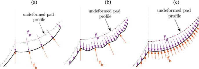

  

  Schematic distribution of air filmbump reaction forces on top foil according to Models 1, 2a, 3, and 2b listed above and summarized in Table 1: a Model 1; b Models 2a and 2b; c Model 3

• Model 2a (Discretely-spaced bumps“continuously distributed” air film forcesbeam model for top foil, Fig. 2b): in this case, top foil sagging in-between bumps is allowed i.e. ${n}_{\mathrm{p}}=m-1\ne {n}_{\mathrm{b}}$.

• Model 3 (“Continuously distributed” bumps“continuously distributed” air film forcesbeam model for top foil, Fig. 2c): this is an alternative to Model 1 for eliminating sagging wherein the bump foil part is reduced to a SEFM (i.e. a continuum of compliance) by putting ${n}_{\mathrm{b}}={n}_{\mathrm{p}}=m-1$.

• Model 2b (Discretely-spaced bumps “continuously distributed” air film forcesshell model for top foil, Fig. 2b): this model differs from 2a with regard to top foil model (shell rather than beam); hence, as in Model 2a, top foil sagging in-between bumps is allowed i.e. ${n}_{\mathrm{p}}=m-1\ne {n}_{\mathrm{b}}$, but the number of elements in air film force vector ${\mathbf{f}}_{\mathrm{p}}$ and bump reaction force vector ${\mathbf{f}}_{\mathrm{b}}$ are ${\left(n-1\right)n}_{\mathrm{p}}$, ${\left(n-1\right)n}_{\mathrm{b}}$ respectively.

The above four models are summarized in Table 1. It is noted that Model 2b (shell top foil) will have less sagging in-between bumps relative to Model 2a (beam top foil). However, it will still have somewhat more sagging than reality since it always assumes line contact between bumps and top foil, whereas in reality, bump deformation changes the contact interface from a line to an area, which tends to reduce sagging in-between bumps [27]. This is the rationale for considering models which eliminate sagging altogether (Models 1 and 3).

Table 1 Different assumptions in modelling the force distribution on the top foil (see also Fig. 2 above)

For a bump foil stiffness per unit area of ${k}_{\mathrm{b}}$ (N/m³), the vector ${\mathbf{f}}_{\mathrm{b}}$ of reaction forces exerted by the bumps on the top foil is determined according to the vector $\widetilde{\mathbf{d}}$ of normalized radial deflections of the top foil at locations corresponding to the bump apexes, using a smoothed bilinear function [20] which is adapted to the present work as follows:

$${\mathbf{f}}_{\mathrm{b}}=\left[\begin{array}{c}\vdots \\ {{F}_{\mathrm{b}}}_{r}\\ \vdots \end{array}\right],\boldsymbol{ }\boldsymbol{ }\widetilde{\mathbf{d}}=\left[\begin{array}{c}\vdots \\ {\widetilde{d}}_{{\varvec{r}}}\\ \vdots \end{array}\right]$$

(14a,b)

where

$${{F}_{\mathrm{b}}}_{r}={{{F}_{\mathrm{bilinear spring}}}_{r}+{F}_{\mathrm{sm}}}_{r}$$

(14c)

${{F}_{\mathrm{bilinear spring}}}_{r}$ is equal to the force from a complex (damped) spring during full contact $\left({\widetilde{d}}_{{\varvec{r}}}\ge \varrho \right)$ and zero otherwise:

$${{F}_{\mathrm{bilinear spring}}}_{r}=\begin{array}{ll}\left({A}_{r}{k}_{\mathrm{b}}\right)\left({\widetilde{d}}_{{\varvec{r}}}+\frac{\eta }{2{\omega }_{\mathrm{ref}}/\varOmega }{\widetilde{d}}_{{\varvec{r}}}^{\mathbf{^{\prime}}}\right)c & \left({\widetilde{d}}_{{\varvec{r}}}\ge \varrho \right)\\ 0 & \left({\widetilde{d}}_{{\varvec{r}}}<\varrho \right)\end{array}$$

(14d)

${A}_{r}$ is the area of the top foil associated with bump no. r, ${A}_{r}{k}_{\mathrm{b}}$ (N/m) is the stiffness of the spring (bump) during full contact and ${A}_{r}{k}_{\mathrm{b}}\eta /{\omega }_{\mathrm{ref}}$ (Ns/m) is the corresponding damping coefficient, where $\eta$ is the hysteretic damping loss factor and ${\omega }_{\mathrm{ref}}$ (rad/s) is the reference frequency used for conversion from hysteretic to viscous damping (in this work ${\omega }_{\mathrm{ref}}=\varOmega$, the rotational speed [20]).

${{F}_{\mathrm{sm}}}_{r}$ is the force from a complex spring that is effective only over the marginal contact state $\left(\left|{\widetilde{d}}_{r}\right|<\varrho \right)$ and has a stiffness that increases linearly from 0 to ${A}_{r}{k}_{\mathrm{b}}$ over the domain $-\varrho <{\widetilde{d}}_{{\varvec{r}}}<\varrho$:

$${{F}_{\mathrm{sm}}}_{r}=\begin{array}{c}\left({A}_{r}{k}_{\mathrm{b}}\right)\left[\left(\frac{1}{4\varrho }{\widetilde{d}}_{{\varvec{r}}}^{2}+\frac{1}{2}{\widetilde{d}}_{{\varvec{r}}}+\frac{\varrho }{4}\right)+\frac{\eta }{2{\omega }_{\mathrm{ref}}/\varOmega }\left(\frac{1}{2\varrho }{\widetilde{d}}_{{\varvec{r}}}+\frac{1}{2}\right){\widetilde{d}}_{{\varvec{r}}}^{\mathbf{^{\prime}}}\right]c \left(\left|{\widetilde{d}}_{r}\right|<\varrho \right) \\ 0 \left(\left|{\widetilde{d}}_{r}\right|\ge \varrho \right)\end{array}$$

(14e)

The term ${{F}_{\mathrm{sm}}}_{r}$ is introduced to smoothen the bilinear term, thus ensuring differentiability. Foil detachment is enabled by setting the smoothing parameter $\varrho$ to a small positive number $(\varrho ={10}^{-3}$ unless otherwise stated). Foil detachment is also enabled, but without smoothing, if $\varrho$ is set to zero. Foil detachment can be completely suppressed (disabled) by setting $\varrho =-\infty$ in Eqs. (14d, 14e).

In the case of using the shell model for the top foil (Model 2b, Table 1), the number of elements in ${\mathbf{f}}_{\mathrm{b}}$ and $\widetilde{\mathbf{d}}$ is ${\left(n-1\right)n}_{\mathrm{b}}$, whereas in the case of using the beam model for the top foil (Models 1, 2a, 3), the number of elements in ${\mathbf{f}}_{\mathrm{b}}$ and $\widetilde{\mathbf{d}}$ will be ${n}_{\mathrm{b}}$. The assumption of variation of top foil deflection with axial position (Model 2b) necessitates consideration of the bump foil as split into a number $\left(n-1\right)$ of strips (that is in theory infinite) placed side by side along the axial length of the bearing since the top foil/bump foil contact model assumes that the top foil will be in contact with the bump foil wherever an element in $\widetilde{\mathbf{d}}$ exceeds $\varrho$. Hence, the supposed added accuracy of considering the top foil as a shell is offset by the corresponding error introduced into the bump foil model if the latter is composed of just one strip (or a few strips).

As stated at the beginning of this section, Eq. (9) stands for a single pad of a given bearing. The equations for all pads $k \left(=1\dots 3\right)$ of each bearing $\gamma$ (A or B) are assembled into the coupled system equations (Eq. (2) as per Eqs. (3a, 3b)).

2.3 Fluid film equations

As in the preceding section, the equations in this section refer to pad no. $k\left(=1\dots 3\right)$ of bearing $\gamma$ (A or B) and the domain of $\theta$ is defined by Eqs. (4a,b and 4c); for clarity, the left-hand superscripts $k$ and right-hand subscripts $\gamma$ are omitted from the following presentation e.g. ${}^{k}{\theta }_{{\mathrm{LE}}_{\gamma }}$, ${}^{k}{\theta }_{{\mathrm{TE}}_{\gamma }}$ are presented as ${\theta }_{\mathrm{LE}}$, ${\theta }_{\mathrm{TE}}$.

The Reynolds equation (RE) for a compressible fluid can be written as

$$B\frac{d}{d\tau }\left(\widetilde{p}\widetilde{h}\right)={\varvec\nabla} \cdot \left(\widetilde{p}{\widetilde{h}}^{3}{\varvec\nabla} \widetilde{p}-\widetilde{p}\widetilde{h}\mathbf{b}\right)$$

(15)

where ${\varvec\nabla} ={\left[\begin{array}{cc}\frac{\partial }{\partial\upxi }& \frac{\partial }{\partial\uptheta }\end{array}\right]}^{\mathrm{T}}$ and $\mathbf{b}={\left[\begin{array}{cc}{b}_{\xi }& {b}_{\theta }\end{array}\right]}^{\mathrm{T}}={\left[\begin{array}{cc}0& B\end{array}\right]}^{\mathrm{T}}$, $B=\frac{6\mu \Omega }{{P}_{a}}{\left(\frac{R}{c}\right)}^{2}$ is bearing number, $\widetilde{h}=\frac{h}{c}$ is non-dimensional film thickness. The boundary conditions applied on pad edges are $\widetilde{p}=1$ and ${\widetilde{p}}{\prime}=0$. Following [8], by defining $\varphi =\left(\widetilde{p}-1\right)\widetilde{h}$, the Reynolds equation can be written as

$$ \varphi^{\prime} + \tilde{h}^{\prime} = \frac{1}{B}{\varvec\nabla} \cdot {\mathbf{r}} $$

(16a)

$$\mathbf{r}=\left[\begin{array}{c}{r}_{\xi }\\ {r}_{\theta }\end{array}\right]=\left(\varphi +\widetilde{h}\right)\left(\widetilde{h}{\varvec\nabla} \varphi -\varphi {\varvec\nabla} \widetilde{h}-\mathbf{b}\right)$$

(16b)

with boundary conditions $\varphi =0$ and ${\varphi }^{\mathrm{^{\prime}}}=0$ on pad edges.

The film thickness $\widetilde{h}$ is given by

$$\widetilde{h}=1+{\widetilde{h}}_{0}\left(\theta \right)+\left[\begin{array}{cc}\mathrm{sin}\theta & -\mathrm{cos}\theta \end{array}\right]{\varvec{\upvarepsilon}}+\widetilde{w}\left(\xi ,\theta \right)=\left[\begin{array}{cccc}1+{\widetilde{h}}_{0}\left(\theta \right)& \mathrm{sin}\theta & -\mathrm{cos}\theta & {\mathbf{v}}_{w}^{\mathrm{T}}\left(\xi ,\theta \right)\end{array}\right]\widehat{\mathbf{h}}={\mathbf{v}}_{h}^{\mathrm{T}}\left(\xi ,\theta \right)\widehat{\mathbf{h}}$$

(17a)

$${\widetilde{h}}_{0}\left(\theta \right)=\frac{{h}_{\mathrm{s}}}{c}\left\{\begin{array}{c}\begin{array}{ll}1-\theta /\beta &\quad \theta \le \beta \\ 0&\quad \theta >\beta \end{array}\end{array}\right.$$

(17b)

$$\widehat{\mathbf{h}}=\left[\begin{array}{c}1\\ {\boldsymbol{\epsilon}}\\ {\mathbf{q}}_{\mathrm{f}}\end{array}\right]$$

(17c)

where ${\widetilde{h}}_{0}\left(\theta \right)$ is the addendum film thickness of sloped region of top foil.

2.4 Galerkin reduction with simultaneous computation of constants (SCC) format

Following the procedure introduced in Sect. 2.3 of [21], the variable $\varphi$ can be expressed as a Galerkin projection of order $N, M$:

$$\begin{aligned} \varphi & = {\mathbf{v}}_{\varphi }^{{\text{T}}} \left( {\xi ,\theta } \right){\boldsymbol{\hat{\upvarphi }}}_{{\text{c}}} = \left( {{\mathbf{g}} \otimes {\mathbf{f}}} \right)^{{\text{T}}} {\boldsymbol{\hat{\upvarphi }}}_{{\text{c}}} \\ & = \left[ {\begin{array}{*{20}c} {g_{1} \left[ {\begin{array}{*{20}c} {f_{1} } & \cdots & {f_{N} } \\ \end{array} } \right]} & \cdots & {g_{M} \left[ {\begin{array}{*{20}c} {f_{1} } & \cdots & {f_{N} } \\ \end{array} } \right]} \\ \end{array} } \right]\left[ \begin{array}{*{20}c} \hat{\varphi}_{\text{c}_1} \\ \vdots \\ \hat{{\varphi}}_{\text{c}_{MN}} \\ \end{array} \right]\\ \end{aligned} $$

(18)

where ${\widehat{\boldsymbol{\upvarphi }}}_{\mathrm{c}}$ is the $NM\times 1$ vector of GR coefficients and ${\mathbf{v}}_{\varphi }$ the corresponding vector of 2D base functions, which is the Kronecker product of vectors $\mathbf{f}={\left[\begin{array}{ccc}{f}_{1}\left(\xi \right)& \cdots & {f}_{N}\left(\xi \right)\end{array}\right]}^{\mathrm{T}}$ and $\mathbf{g}={\left[\begin{array}{ccc}{g}_{1}\left(\theta \right)& \cdots & {g}_{M}\left(\theta \right)\end{array}\right]}^{\mathrm{T}}$ containing orthogonal analytic functions in the respective $\xi$, $\theta$ directions that satisfy boundary conditions of $\varphi$ for a pad ($\varphi =0$ on pad edges). These elementary (1D) base functions are chosen as

$${f}_{i}\left(\xi \right)=\mathrm{cos}\left(\left(2i-1\right)\frac{\pi R\xi }{L}\right), {g}_{j}\left(\theta \right)=\mathrm{sin}\left(j\pi \frac{\theta -{\theta }_{\mathrm{LE}}}{{\theta }_{\mathrm{TE}}-{\theta }_{\mathrm{LE}}}\right)$$

(19)

Following [8], the GR projection of Eq. (16a) is obtained by multiplying both sides by the $NM\times 1$ vector of 2D base functions ${\mathbf{v}}_{\varphi }$ (see Eq. (18)) and integrating over the full extent of the pad:

$$\left(\int {\mathbf{v}}_{\varphi }{\mathbf{v}}_{\varphi }^{\mathrm{T}}\mathrm{d}\mathcal{A}\right){\widehat{\boldsymbol{\upvarphi }}}_{\mathrm{c}}^{\mathbf{^{\prime}}}=-\frac{1}{B}\int {({\mathbf{v}}_{\varphi }^{\left(\xi \right)}{r}_{\xi }+\mathbf{v}}_{\varphi }^{\left(\theta \right)}{r}_{\theta })\mathrm{ d}\mathcal{A}-\int {\mathbf{v}}_{\varphi }{\widetilde{h}}^{\mathrm{^{\prime}}}\mathrm{ d}\mathcal{A}$$

(20)

Applying numerical integration to Eq. (20) as explained in Sect. 2.3.1 of [21], will result in a set of $NM$ first order ODEs that defines the Reynolds equation on the domain of a single pad:

$${\widehat{\mathbf{\varvec{\upvarphi }}}}_{\mathrm{c}}^{\mathbf{^{\prime}}} ={\mathbf{M}}^{-1}\left(-\frac{1}{B}{{\mathbf{V}}_{\varphi }^{\left(\xi \right)}}^{\mathrm{T}}\mathbf{A}{\mathbf{r}}_{\xi }-\frac{1}{B}{{\mathbf{V}}_{\varphi }^{\left(\theta \right)}}^{\mathrm{T}}\mathbf{A}{\mathbf{r}}_{\theta }-{\mathbf{V}}_{\varphi }^{\mathrm{T}}\mathbf{A}{\mathbf{h}}{\prime}\right)$$

(21a)

$${\mathbf{r}}_{\alpha }=\left({\varvec{\upvarphi }}+\mathbf{h}\right).*\left(\mathbf{h}.*{{\varvec{\upvarphi }}}^{\left(\alpha \right)}-{\varvec{\upvarphi }}.*{\mathbf{h}}^{\left(\alpha \right)}-{b}_{\alpha }{1}_{nm\times 1}\right), \left(\alpha =\xi ,\theta \right)$$

(21b)

The above formulation is referred as the simultaneous computation of constants (SCC) format [21] since the integrations of Eq. (20) required to determine the constants within the right hand side of Eq. (21a) are evaluated simultaneously with the solution of Eq. (2) via the matrix $\mathbf{A}$ of integration weights associated with each point of the quadrature sampling grid (Eq. (13b)). The remaining matrices in Eq. (21a, 21b) are defined as follows

$${\varvec{\upvarphi }}={\mathbf{V}}_{\varphi }{\widehat{\varvec{\upvarphi }}}_{\mathrm{c}}$$

(22a)

$$\mathbf{h}={\mathbf{V}}_{h}\widehat{\mathbf{h}}$$

(22b)

$$\mathbf{M}={\mathbf{V}}_{\varphi }^{\mathrm{T}}\mathbf{A}{\mathbf{V}}_{\varphi }$$

(22c)

and the matrices ${\mathbf{V}}_{\varphi }$, ${\mathbf{V}}_{h}$ and their derivatives with respect to $\alpha$ ($\alpha =\xi ,\theta$), are built by concatenating ${\mathbf{v}}_{\varphi }\left(\xi ,\theta \right)$, ${\mathbf{v}}_{h}\left(\xi ,\theta \right)$ evaluated on points of $n\times m$ sampling grid:

$${\mathbf{V}}_{\varphi }={\left[\begin{array}{ccc}{\mathbf{v}}_{\varphi }\left({\xi }_{{\mathrm{P}}_{1}},{\theta }_{{\mathrm{P}}_{1}}\right)& \cdots & {\mathbf{v}}_{\varphi }\left({\xi }_{{\mathrm{P}}_{nm}},{\theta }_{{\mathrm{P}}_{nm}}\right)\end{array}\right]}^{\mathrm{T}}$$

(23a)

$${\mathbf{V}}_{h}={\left[\begin{array}{ccc}{\mathbf{v}}_{h}\left({\xi }_{{\mathrm{P}}_{1}},{\theta }_{{\mathrm{P}}_{1}}\right)& \cdots & {\mathbf{v}}_{h}\left({\xi }_{{\mathrm{P}}_{nm}},{\theta }_{{\mathrm{P}}_{nm}}\right)\end{array}\right]}^{\mathrm{T}}$$

(23b)

where ${\mathbf{v}}_{\varphi }$, ${\mathbf{v}}_{h}$ are given by Eqs. (18) and (17a) respectively.

The vector of air film state variables for the domain of the pad under consideration is ${}^{k}{\mathbf{s}}_{{\mathrm{a}}_{\gamma }}={\widehat{\varvec{\upvarphi }}}_{\mathrm{c}}$, and ${}^{k}{{\varvec{\upchi}}}_{{\mathrm{a}}_{\gamma }}\left(\mathbf{s}\right)$ will be the right hand side (RHS) of Eq. (21a). The equations for all pads $k \left(=1\dots 3\right)$ of each bearing $\gamma$ (A or B) are assembled into the coupled system equations (Eq. (2) as per Eqs. (3a, 3b)).

2.5 Finite Difference (FD) discretization

Expanding the terms in Eq. (16a) and evaluating them on a FD sampling grid consisting ${n}_{\xi }\times {m}_{\theta }$ points on $\xi{-}\theta$ plane leads to the FD-discretized version of Reynold Equation as follows:

$${\varvec{\upvarphi }}^{\mathrm{^{\prime}}}=\frac{1}{B}[\left({\varvec{\upvarphi }}^{\left(\xi \right)}+{\mathbf{h}}^{\left(\xi \right)}\right).*\left(\mathbf{h}.*{\varvec{\upvarphi }}^{\left(\xi \right)}-{\varvec{\upvarphi }}.*{\mathbf{h}}^{\left(\xi \right)}-{b}_{\xi }{\mathbf {1}}_{{n}_{\xi }{m}_{\theta }\times \mathbf{1}}\right)$$

$$+\left({\varvec{\upvarphi }}^{\left(\theta \right)}+{\mathbf{h}}^{\left(\theta \right)}\right).*\left(\mathbf{h}.*{\varvec{\upvarphi }}^{\left(\theta \right)}-{\varvec{\upvarphi }}.*{\mathbf{h}}^{\left(\theta \right)}-{b}_{\theta }{\mathbf {1}}_{{n}_{\xi }{m}_{\theta }\times 1}\right)+$$

$$\left({\varvec{\upvarphi }}+\mathbf{h}\right).*\left(\mathbf{h}.*{{\varvec{\upvarphi }}}^{\left(\xi \xi \right)}+\mathbf{h}.*{{\varvec{\upvarphi }}}^{\left(\theta \theta \right)}-{\varvec{\upvarphi }}.*{\mathbf{h}}^{\left(\xi \xi \right)}-{\varvec{\upvarphi }}.*{\mathbf{h}}^{\left(\theta \theta \right)}\right)]-{\mathbf{h}}^{\mathrm{^{\prime}}}$$

(24)

where $\mathbf{h}$ is the vector of the air film thickness values at the grid sampling points and is still determined using Eqs. (22b) and (23b), as are the vectors of air film thickness derivatives with respect to $\theta$ and $\xi$) since ${\mathbf{V}}_{h}$ does not use GR base functions. It is also noted that in the present case of FD, ${n}_{\xi }$, ${m}_{\theta }$ are used instead of $n$, $m$ in the equation for ${\mathbf{V}}_{h}$ (Eq. (23b)) since the resolution of the sampling grid used in FD is not necessarily the same as the quadrature sampling grid used in GR. $\mathbf{\varphi }$ in Eq. (22a) is the vector of air film state variables $\varphi$ at the grid sampling points, and the vectors of the spatial derivatives of $\varphi$ are determined using finite difference matrices as follows:

$${\varvec{\upvarphi }}={\left[\begin{array}{ccc}\varphi \left({\xi }_{{\mathrm{P}}_{1}},{\theta }_{{\mathrm{P}}_{1}}\right)& \cdots & \varphi \left({\xi }_{{\mathrm{P}}_{{n}_{\xi }{m}_{\theta }}},{\theta }_{{\mathrm{P}}_{{n}_{\xi }{m}_{\theta }}}\right)\end{array}\right]}^{\mathrm{T}}$$

(25a)

$${\varvec{\upvarphi }}^{(\alpha )}={\overline{\mathbf{V}} }_{\varphi }^{\left(\alpha \right)}{\varvec{\upvarphi }},{\varvec{\upvarphi }}^{(\alpha \beta )}={\overline{\mathbf{V}} }_{\varphi }^{\left(\alpha \beta \right)}{\varvec{\upvarphi }}\left(\alpha =\xi ,\theta \right)$$

(25b)

The vector of air film state variables for the domain of the pad under consideration is ${}^{k}{\mathbf{s}}_{{\mathrm{a}}_{\gamma }}={\varvec{\upvarphi }}$, and ${}^{k}{{\varvec{\upchi}}}_{{\mathrm{a}}_{\gamma }}\left(\mathbf{s}\right)$ will be the right hand side (RHS) of Eq. (24). The equations for all pads $k \left(=1\dots 3\right)$ of each bearing $\gamma$ (A or B) are assembled into the coupled system equations (Eq. (2) as per Eqs. (3a, 3b)).

2.6 Computational approach

Once Eq. (1) is assembled as per Eq. (2), solution at a given rotational speed is performed by way of.

• static equilibrium, stability and modal analysis (SESMA) [11, 21], involving the following steps

  • static equilibrium solution of the nonlinear system, obtained by setting ${\mathbf{s}}^{\mathrm{^{\prime}}}=0$ in Eq. (1) and solving the nonlinear algebraic equations for the static equilibrium condition (SEC);

  • free linearized vibration analysis about the SEC at each individual speed over a range through an eigenvalue analysis of the Jacobian of the right hand side of Eq. (1), in order to derive the Campbell diagrams and stability plots.

• transient nonlinear dynamic analysis (TNDA) of Eq. (1) using an implicit (stiff) solver (e.g. ode15s in Matlab)—this involves time integration from prescribed initial conditions at a given rotational speed (with or without rotational unbalance) over a sufficiently long period for the initial transients to decay and a steady-state response achieved.

Both TNDA and SESMA require the Jacobian of the dynamical system. With the GR transformation of the RE, the size of the Jacobian $\mathbf{J}$ of the present system will be $\left(6NM+12{m}_{\mathrm{f}}+2H\right)\times \left(6NM+12{m}_{\mathrm{f}}+2H\right)$ since each of the two bearings has three pads, thus yielding $3NM$, $3\times 2{m}_{\mathrm{f}}$ state variables for the air film and foil structure respectively of each bearing. On the other hand, if FD was used to transform the RE, there will be $3{n}_{\xi }{n}_{\theta }$ equations for the air film of each bearing and the size of $\mathbf{J}$ would therefore be $\left({6n}_{\xi }{n}_{\theta }+12{m}_{\mathrm{f}}+2H\right)\times \left({6n}_{\xi }{n}_{\theta }+12{m}_{\mathrm{f}}+2H\right)$ where ${n}_{\xi }{\times n}_{\theta }$ is the effective size of the FD grid of one pad (considering only one symmetric half of bearing and excluding boundaries [20]). The condensation (and consequent computational savings) afforded by GR is based on the premise that $NM\ll {n}_{\xi }{n}_{\theta }$ for a given degree of accuracy.

For efficient computation, the Jacobians are determined from functions supplied to the computational solver. In the case of GR, the functional expressions of the Jacobian pertaining to a single pad of each bearing are those already given in [21] (Sect. 2.4.1).

3 Results and discussion

The rotor-bearing system in Fig. 1 with the dimensions and properties listed in Table 2 [6] is used for numerical analysis. This system was chosen so that the study's results could be compared to the experimental and theoretical results of Larsen and Santos [6], as well as further theoretical results of Larsen et al. [28] and Bonello [11]. In this system, the rotor is assumed to be rigid over the operating speed range (up to ~ 30 krpm), hence there are 4 degrees of freedom, which means that $H=4$ modes are used to transform the equations of motion of the rotor subsystem (Eq. (5)) [11]. The analysis in [6, 11, 28] used FE or FD for the air film domain, rather than order reduction. Moreover, the analysis in [6, 11, 28] did not model detachment of top foil from bump foil and were based on the simple elastic foundation model (SEFM) for the foil with the Gümbel condition applied in order to correct for ignoring top foil detachment [6, 11] (this is done during the evaluation of the bearing forces in Eq. (7) by identifying sub-atmospheric regions (${\widetilde{p}}_{\gamma }<1$) and resetting them to atmospheric (${\widetilde{p}}_{\gamma }=1$)). The Campbell diagram produced by Bonello in [11] (showing variation of the natural frequency of damped linearized vibration about the static equilibrium condition of the nonlinear system over a range of speeds) is reproduced in Fig. 3. Modes 1, 3 are translational modes where the mode shape of the rotor is cylindrical, while modes 2, 4 are pitching modes, where the mode shape of the rotor is double-conical (node approximately at the midpoint). The simulation in [11] for the vibration in mode 1 at 30krpm is shown in Fig. 3 (showing modal vibration at bearing A). Such modes where also predicted for the same system by von Osmanski and Santos in [13]. An important point to note from Fig. 3 (and the full results for the modes in [13] and [11]) is that the foil vibration is not realistic since there is no vibration at the free end of the pad (where the pressure is atmospheric)—this is a limitation of the SEFM model that is overcome by the foil detachment model as shown later.

Table 2 Parameters of the Siemens foil bearing test-rig [6]—please refer to Fig. 1b

Fig. 3

Campbell diagram for the system as predicted with SEFM/Gümbel foil model in [11] (inset shows predicted modal vibration at bearing A in Campbell mode 1 at 30 krpm)

In the present work, top foil detachment is enabled by setting the smoothing parameter $\varrho ={10}^{-3}$ in Eqs. (14d, 14e); top foil detachment can be disabled (suppressed) by setting $\varrho =-\infty$ (this latter setting is only used in Sect. 3.1 for verification purposes).

When referring to FD, the full grid for each of the three pads is $15\times 47$ (i.e. effective grid of $7\times 47$) and when referring to GR, the quadrature sampling grid [21] for each pad is the same as the full grid per pad considered for FD.

Unless otherwise stated, the top foil is modelled as a curved beam and the number of top foil component modes is ${m}_{\mathrm{f}}=20$ (justified in Figure A1 of Appendix).

3.1 Preliminary verification

The modal top foil/bilinear bump foil model used in the present work can be reduced as close as possible to the SEFM/Gümbel model of [6, 11, 28] by disabling the top foil detachment and then applying the Gümbel condition. In that situation, the only difference from the SEFM/Gümbel model will be the inertia and bending stiffness of the top foil (embedded in the modal model), which are not influential [20]. Note that when detachment is enabled, the Gümbel condition is of course not applied since the air film pressures will self-adjust accordingly.

To verify the modal, non-detachable/Gümbel model based on GR, the steady-state responses at bearing A for the stable speed of 20 krpm under two different levels of rotor unbalance were computed by TNDA and compared against the corresponding literature results [28] that were obtained by considering SEFM/Gümbel and Finite Element (FE) discretization of the air film. As shown in Fig. 4, the predictions from the present work exhibit nearly identical behaviour as those from [28] as the level of rotor unbalance increases (sub-synchronous vibrations emerging as rotor unbalance is doubled).

Fig. 4

Verification of predicted journal steady state response at bearing A (frequency spectra and orbits) for 20 krpm under two different unbalance levels: (a, b) unbalance at each bearing of $20\,\mathrm{g\,mm}$, 180° out of phase i.e. ${u}_{\mathrm{A}}=20\,\mathrm{g\,mm},$ ${u}_{\mathrm{B}}=-20\,\mathrm{g\,mm}$ (a GR $\left(\mathrm{3,16}\right)$, b prediction from [28] using FE for air film); (c, d) ${u}_{\mathrm{A}}=40\,\mathrm{g\,mm},$ ${u}_{\mathrm{B}}=-40\,\mathrm{g\,mm}$ (c GR $\left(\mathrm{3,16}\right)$, d prediction from [28] using FE for air film) (for the results in this figure, ${k}_{\mathrm{b}}=9.26\times {10}^{9}$ N/m.³ [28] i.e. slightly different from that quoted in Table 2)

Figure 5 compares the no-detachment/Gümbel model results (Fig. 5a, b) with the results from the detachment model (Fig. 5c, d) for the case of the transient (TNDA) response from the default initial state (journal initially concentric with bearing housing) at zero unbalance and 20 krpm. Figure 5 also presents the convergence of the corresponding time response trajectories for different GR orders $N,M$. As the graphs show, $N=3,M=16$ is an appropriate order to use for the problem in both cases. Another point to note is the effect of applying Gümbel condition on the result for the trajectory of the journal. Even though the foil deformations in Fig. 5a, b (no detachment) are different from those in Fig. 5c, d (detachment allowed), the corresponding journal trajectories are similar. This provides evidence that, for the present system, the Gümbel condition is a good correction for the journal trajectory prediction if using a model that ignores top foil detachment.

Fig. 5

Convergence of GR-computed time response of journal trajectory (0.2 s duration) at 20 krpm, no unbalance, for different GR orders $\left(N,M\right)$: (a, b) no detachment/Gümbel; (c, d) with detachable foil

Figure 6 compares the same transient (TNDA) response from the default initial state at zero unbalance and 20 krpm as predicted by Finite Difference (FD) with that predicted by GR for both models (no-detachment/Gümbel, detachment). The correlation between FD and GR is seen to be excellent for both cases.

Fig. 6

Comparison of GR and FD for detachable foil model and no detachment/Gümbel model (20 krpm, no unbalance)

It should be noted that both detachable and non-detachable results of Sect. 3.1 and 3.2 are based on model 1 (see Table 1 and Fig. 2a). For the first part of the study (this section and next Sect. 3.2), the emphasis is on this model, which does not allow sagging to occur in areas between the bumps. This model for force distribution has been previously used in [21] to investigate the behavior of a system with single pad bearings. Sections 3.3–3.5 will consider the other force distribution models in Table 1.

3.2 Concentrated air film forces and discrete bumps (Model 1, Fig. 2a, Table 1)

Using Model 1 for the top foil force distribution with foil detachment, static equilibrium, stability and modal analysis (SESMA) is performed over a range of speeds, revealing the unfiltered eigenmodes’ damping ratios vs speed maps for both GR and FD (see Fig. 7). Each point at a given rotating speed represents an eigenmode of the free linearized vibration of the multi-domain system about its SEC. The vast proportion of these modes involve negligible vibration of the rotor and need to be filtered out in order to extract the Campbell diagram (which should result in four modes of the rotor bearing system at each speed, as was shown in Fig. 3) following the procedure of [11]. However, use of Model 1 for the force distribution on the top foil revealed an issue not encountered before—namely, instability (negative damping ratio) of the static equilibrium condition at speeds below around 14 krpm (GR), or below around 10 krpm (FD) (identified by the negative damping ratio branches in the low speed range of Fig. 7). It was also ascertained that such low speed instability with Model 1 persisted with higher resolution FD or higher order GR.

Fig. 7

Unfiltered eigendamping vs speed map for perturbations about the SEC using Model 1 (Table 1): a using GR (3,16); b using FD

Unlike the unstable mode branch at the higher end of the speed range (which is a genuine part of the Campbell diagram), the eigenmodes responsible for the low speed instabilities are “pad flutter”-type modes involving negligible vibration of the rotor and considerable vibration in the most-loaded pad of the bearings, as shown in Fig. 8.

Fig. 8

Unstable modes (perturbations about SEC) at speed of 9 krpm using GR (3,16) for top foil force distribution Model 1 (Table 1) (different instances during the vibration are indicated by different colours/line types for top foil, and different colours/markers for journal orbit)

For this reason, to export such unstable flutter modes from the unfiltered eigenfrequency vs speed map to the Campbell diagram, the filtering criterion was modified to allow them to pass, even though they fail the usual filtering criterion (which imposes a minimum limit on the journal amplitude [11]). Figures 9a, b and 10a, b show the Campbell and modal stability plots for GR and FD respectively, each with superimposed unstable top foil flutter modes. The top foil flutter modes in Figs. 9, 10 and 8 at first glance appear similar to those encountered in [21] for the case of single (360°) pad FABs. However, unlike the flutter modes in [21], the present flutter modes are reliably considered to be artifacts of the numerical modelling procedure (i.e. they have no physical basis), for the following reasons:

• Their frequencies (in the kHz) are very much higher than those of the four Campbell modes, in contrast with the case in Fig. 8c, d of [21] where the pad flutter mode frequency was of an order of magnitude that was similar to those of the Campbell mode frequencies.

• The top foil flutter frequencies and damping ratios obtained by GR (Fig. 9) are significantly different from those obtained by FD (Fig. 10) (and both will be affected by the assumed number of modes used for the top foil), whereas the normal (Campbell) modes obtained by GR and FD are in close agreement.

• The top foil flutter modes in the present case can be completely eliminated by changing the top foil force distribution model from Model 1 to any one of the other three models in Table 1, as will be shown in the following sections.

Fig. 9

Campbell diagram and modal damping plot for top foil force distribution Model 1 (Table 1) using GR (3,16) with superimposed unstable top foil flutter modes

Fig. 10

Campbell diagram and modal damping plot for Model 1 (Table 1) using FD with superimposed unstable top foil flutter modes

Such artificial (purely numerical) instability prevented convergent TNDA results over its speed regime. Although convergent TNDA results outside the flutter’s speed regime were achievable in certain cases at low unbalance (e.g. the results in Figs. 4, 5), continuing with Model 1 to obtain waterfall graphs over the full speed range of the study (5.4 to 30 krpm) was considered futile.

With regard to the four Campbell modes in Fig. 9 or Fig. 10, these are consistent with Fig. 3, and the salient differences are the abrupt shifts in frequency and damping in the present case, which occur whenever the state of contact of the top foil with a particular bump changes with speed, as already noted in [21] for the case of single (360°) pad FABs.

In conclusion, despite the fact that top foil distribution Model 1 (Table 1) worked well for the single (360°) pad FAB rotor system in [21], it causes numerical problems when applied to the present 4-degree-of-freedom system fitted with three-pad FABs.

3.3 Distributed air film forces and discrete bumps (Model 2a, Fig. 2b, Table 1)

Model 2a (Table 1) allows sagging in between bumps. In order to reduce this sagging effect, the number of component beam modes used for the modal superposition of the top foil is reduced to ${m}_{\mathrm{f}}=16$.

Following free vibration analysis about the SEC using both GR and FD for the air film domain, the corresponding unfiltered eigenmodes damping ratios vs speed maps are shown in Fig. 11. Comparing with the equivalent results obtained in the previous section using Model 1 (Fig. 7), the numerical problem of artificial flutter modes at low speeds is seen to have disappeared using Model 2a (this finding also holds when the number of top foil component modes is reverted to ${m}_{\mathrm{f}}=20$).

Fig. 11

Unfiltered eigendamping vs speed map for Model 2a (Table 1): a using GR (3,16); b using FD

The Campbell diagram and its corresponding modal damping graphs are extracted from the eigenvalue analysis and are plotted in Fig. 12. These graphs are seen to be the same as those of the Campbell (i.e. non-flutter) modes in Fig. 9 or Fig. 10, further illustrating the elimination of the aforementioned problem of artificial instabilities. The 1 EO line intersects with modes 2, 3 and 4 at about 110 Hz, 155 Hz and 193 Hz or 6.9, 9.6, 11.7krpm, respectively. Although the 1 EO line intersects with mode 3, but the intersection point is a reverse whirl mode which is not excited by rotational unbalance (which is the normal source of 1 EO excitation). These critical speeds agree with the values already reported in [6, 11].

Fig. 12

Campbell diagram and modal damping for top foil force distribution Model 2a (Table 1) using GR (3,16)

The onset of instability speed (OIS) is 29.14 krpm, which is close to that predicted in the literature using the SEFM/Gümbel-corrected (no-detachment) foil model (30.5 krpm) [11] (see Fig. 10 of [11]). Figure 13(a-d) shows the results for the vibration in each of the four modes at 29.14 krpm. The vibration of the rotor in each of these modes is seen to agree with those published in the literature (e.g. Figure 12–15 of [11]). However, the top foil vibrations in Fig. 13(a-d) are evidently different from those in the literature (e.g. compare Fig. 13a with Fig. 12 of [11]), and give the more realistic response since the Gümbel correction is only effective on the journal response and the SEFM model inherently constrains the top foil deflection to zero at the free ends at all times. It is noted that Figs. 13(b,c) show differences in the journal orbits at the two bearings A, B; this is attributed to the slight asymmetry in the rig (${l}_{\mathrm{A}}$, ${l}_{\mathrm{B}}$ slightly unequal in Table 2).

Fig. 13

Campbell modes at speed of 29.14 krpm for top foil force distribution Model 2a (Table 1) using GR (3,16) (different instances during the vibration are indicated by different colours/line types for top foil, and different colours/markers for journal orbit)

The waterfall diagram for the steady-state response of the nonlinear system at low unbalance (${u}_{\mathrm{A}}=2.5\mathrm{ g \cdot mm}\; {\mathrm {and}}\; {u}_{\mathrm{B}}=-2.5 \mathrm{g mm}$) with GR (3,16) is shown in Fig. 14. As in [6], this was done by performing TNDA at fixed speeds over a range of speeds; as in [6], at each speed the TNDA was performed over 1s, with the first 0.2 s (transient stage) neglected from the FFT. It is seen that there is no sub-synchronous vibration in this graph until around 30 krpm, when a frequency of 100 Hz rises into prominence. This is in accordance with the Campbell diagram in Fig. 12 which predicts an OIS of 29 krpm due to mode 1 becoming unstable at this speed where its frequency is around 100 Hz. Another important thing is that waterfall diagram shows two resonance (critical) speeds at around 6.9 and 11.7krpm, which are consistent with those already reported from Campbell diagram in Fig. 12. This graph is in close agreement with what has been reported experimentally and theoretically (using SEFM/Gümbel) in [6].

Fig. 14

Waterfall diagram for rotor unbalance of ${u}_{\mathrm{A}}=2.5\,mathrm{ g \,mm} \,\text{and}\, {u}_{\mathrm{B}}=-2.5\,\mathrm{g\,mm}$ with Model 2a (Table 1) using GR (3,16)

The next waterfall diagram, Fig. 15, is for the case when the unbalance is set to be ${u}_{\mathrm{A}}=40\mathrm{ g \cdot mm \; and}\; {u}_{\mathrm{B}}=-2.5 \mathrm{g \cdot mm}$. Now, due to the significantly raised level of unbalance, a sub-synchronous frequency component appears from 9 krpm (i.e. much lower than the OIS). At approximately 11.4 krpm, the sub-synchronous frequency component bifurcates into a pair of sub-synchronous frequency components which tend to increase in amplitude until they vanish completely at 13.5krpm. This phenomenon is in agreement with that reported in the corresponding waterfall diagram of Fig. 7 of ref [6] (that was evaluated by SEFM/Gümbel foil model). It is noted however that in ref [6], the bifurcated sub-synchronous frequency pair re-emerges over a short speed range of 17.6 krpm to 19.1 krpm before completely vanishing again.

Fig. 15

Waterfall diagram for rotor unbalance of ${u}_{\mathrm{A}}=40\mathrm{ g mm}\;{\mathrm {and}}\; {u}_{\mathrm{B}}=-2.5 \mathrm{g mm}$ with Model 2a (Table 1) using GR (3,16)

Figure 16 shows the nonlinear steady-state orbital vibration for different level of unbalance at different speeds. At low unbalance levels, the rotor response is nearly linear, consisting of the synchronous frequency component and therefore resulting in elliptical orbits, as can be seen in Fig. 16a when the applied unbalance at the speed of 11.4 krpm is ${u}_{\mathrm{A}}=10\mathrm{ g \cdot mm}\; {\mathrm {and}}\;{u}_{\mathrm{B}}=-2.5\mathrm{ g}\cdot\mathrm{m}$. Increasing the rotor unbalance to ${u}_{\mathrm{A}}=40\mathrm{ g \cdot mm}\;{\mathrm {and}}\;{u}_{\mathrm{B}}=-2.5\mathrm{ g \cdot mm \; at \; speeds \; of }11.4 \; \mathrm{ krpm \; and\; }9 \; \mathrm{ krpm}$ will lead to the emergence sub-synchronous frequency components and complicated pattern for the orbit, as can be seen in Fig. 16 (b,c). On the other hand, applying the same level of unbalance at the speed of 25.2 krpm, the sub-synchronous frequency components disappear, as evident from the elliptical orbits in Fig. 16 (d). This behavior is in agreement with that observed in the simulations of reference [6]. The inducing of non-synchronous vibration under high unbalance has been qualitatively explained as a Duffing oscillator effect from the foil pad (stiffness hardening in the bearing force-shaft displacement relation) by Balducchi et al. [5], using a highly simplified model that neglected the air film, and which gave very limited agreement with experiment.

Fig. 16

Nonlinear steady-state rotor orbits for Model 2a (Table 1) using GR (3,16): a

${u}_{\mathrm{A}}=10\,\mathrm{g\,mm}$ and ${u}_{\mathrm{B}}=-2.5 \mathrm{g mm \, at \, speed\, of }11.4\;\mathrm{ krpm}$, b ${u}_{\mathrm{A}}=40\mathrm{ g mm}\;{\mathrm {and}}\; {u}_{\mathrm{B}}=-2.5 \mathrm{g mm \; at \; speed \; of }\; 11.4\; \mathrm{ krpm}$, c ${u}_{\mathrm{A}}=40\mathrm{ g mm }\;{\mathrm {and}}\; {u}_{\mathrm{B}}=-2.5 \mathrm{g mm \; at \; speed \; of }\; 9 \; \mathrm{ krpm}$, d ${u}_{\mathrm{A}}=40\mathrm{ g mm }\;{\mathrm {and}}\; {u}_{\mathrm{B}}=-2.5 \mathrm{g mm\; at \; speed \; of }\; 25.2\; \mathrm{ krpm}$

The use of top foil force distribution Model 2a instead of Model 1 (see Table 1) has resulted in the ability to generate validated TNDA results. However, the distribution of air film forces in-between the discretely spaced bumps allowed the top foil to sag in the areas between the bumps, and this was considered to be the cause of numerical convergence issues during TNDA at certain speeds when the number of component modes used in the top foil modal superposition exceeded 19.

For this reason, two further top foil force distribution models are investigated that eliminate or reduce sagging, while keeping a continuous distribution of air film forces—Model 3, Model 2b (see Table 1).

3.4 Distributed air film forces and continuously distributed bumps (Model 3, Fig. 2c, Table 1)

With reference to Table 1, top foil force distribution Model 3 eliminates sagging completely under a continuous distribution of air film forces, by assuming a similarly continuous distribution of bump apexes along the circumferential direction. In reality, the bump apexes are discretely spaced according to the circumferential pitch (${S}_{\mathrm{b}}$ in Table 2), but the top foil detachment model based on this force distribution model is expected to give results that are the closest to the published SEFM/Gümbel results of [6, 11] since the SEFM is a continuously distributed compliance model for the bump foil. This is evident from the Campbell diagram of Fig. 17, which unlike that of Fig. 12 has no abrupt shifts caused by changes in contact state of a bump, and is therefore closer to the one from the literature [11]. (The small discontinuities in Fig. 17 are caused by a change in the contact state of the bumps; since, in Model 3, the bumps are spaced at the sampling grid resolution, the change in contact state happens over an increased number of positions, resulting in a “smoother” effect).

Fig. 17

Campbell diagram and modal damping for Model 3 (Table 1) using GR (3,16)

As shown in Fig. 18, there is no difference in top foil deformation between the Model 2a and Model 3 of Table 1 when the number of top foil modes considered is up to 16, but as this number increases, sagging begins to appear in-between the discretely-spaced bumps in Model 2a. The waterfall diagrams in Fig. 19a, b show that, unlike the case with Model 2a, increasing the number of top foil component modes from 16 to 24 does not result in numerical convergence issues at any speed.

Fig. 18

Static equilibrium condition at bearing A at a certain speed—comparison between Models 2a and 3 (Table 1) using GR (3,16): a with 16 top foil modes b with 20 top foil modes

Fig. 19

Waterfall diagram for rotor unbalance of ${u}_{\mathrm{A}}=40\mathrm{ g \cdot mm}\; \mathrm { and}\; {u}_{\mathrm{B}}=-2.5 \mathrm{g\cdot mm}$, with Model 3 (Table 1): a with 16 modes b with 24 modes

3.5 Distributed air film forces and discretely-spaced bumps using shell model for top foil (Model 2b, Fig. 2b, Table 1)

With reference to Table 1, top foil force distribution Model 2b is expected to reduce top foil sagging under a continuous distribution of air film forces, in comparison to Model 2a, by considering a shell model for the top foil rather than beam model. Although the top foil of each pad is supported by just four strips of bump foil placed side by side axially (i.e. circumferentially split, as per Fig. 2.3 of [15], it is noted that the contact model assumes that the top foil is in contact with a bump foil apex at all points for which the top foil deflection exceeds the set threshold $\varrho$ (in reality this would only be physically possible if the bump foil was split into a very large number of strips placed side by side over the axial length of the bearing).

As shown in Fig. 20, the number of top foil mode shapes required to achieve convergence when using the shell model is at least 30, and with this number, sagging is negligible (in contrast to the use of beam modes for the top foil—see Fig. 21). Indeed, with a shell model for the top foil, the number of modes required to observe sagging is much higher than the number required to achieve convergence, as shown in Fig. 21b, where it is seen that sagging is only visible when 100 modes are used.

Fig. 20

Convergence study for different number of modes using GR (3,16) with Model 2b (Table 1) at 20 krpm, no unbalance

Fig. 21

Static equilibrium condition at bearing A at a certain speed: a comparison between results of Models 2a, 3 and 2b (Table 1) using GR (3,16); b using different number of shell mode shapes with Model 2b

Hence, the waterfall graph of the steady-state unbalance response could be achieved without any numerical convergence issues with this number of shell modes (30) for Model 2b, as shown in Fig. 22 (in contrast to Model 2a, where the number of top foil beam modes had to be limited to 19 to avoid convergence issues arising from excessive sagging).

Fig. 22

Waterfall diagram for rotor unbalance of a ${u}_{\mathrm{A}}=2.5\mathrm{ g mm }\;{\mathrm {and}}\; {u}_{\mathrm{B}}=-2.5 \mathrm{g mm}$ b ${u}_{A}=40\mathrm{g mm}\;{\mathrm {and}}\; {u}_{B}=-2.5 \mathrm{g mm}$ using Model 2b (Table 1) with 30 shell modes for top foil

The only disadvantage of using shell model (Model 2b) is that the time required to obtain the full waterfall graph is longer than when using the beam model (Model 2a), as shown in the following section. It should be noted however that, as shown in Fig. 20, considering 16 modes with Model 2b appears to be a good approximation. This is further illustrated in Fig. 23, which compares the FFTs of the steady-state unbalance response for selected speeds, taking into account 16 and 30 modes, and shows that the use of 16 modes does not significantly compromise the accuracy of the results, while providing considerable time saving.

Fig. 23

Steady-state response at bearing A for rotor unbalance of ${u}_{\mathrm{A}}=40\mathrm{ g mm}\;{\mathrm {and}}\; {u}_{\mathrm{B}}=-2.5 \mathrm{g mm}$ at different speeds with Model 2b (Table 1) and different numbers of top foil component modes: 16 shell modes (solid blue line); 30 shell modes (dashed red line)

3.6 CPU times

Table 3 shows the time required to obtain the full waterfall graph for the case of ${u}_{\mathrm{A}}=40\mathrm{ g \cdot mm }\; {\mathrm {and}} \;{u}_{\mathrm{B}}=-2.5\,\mathrm{g \cdot mm}$ using top foil force distribution Model 2a and Model 3 (Table 1) for both FD and GR methods. It is clear that, using GR transformation instead of FD, reduces the computational cost by around half (reduction of ~ 51% for both Model 2a and Model 3).

Table 3 Computational efficiency of GR compared to FD in terms of CPU time to obtain waterfall diagrams for rotor unbalance of ${u}_{\mathrm{A}}=40 \mathrm{g mm} \; \mathrm{and}\; {u}_{\mathrm{B}}=-2.5 \mathrm{g mm}$ (using 16 beam modes for top foil; CPU times are averages of three runs on the same machine, which was restarted after each run)

Using Model 2b (with 30 shell modes for top foil) instead of Model 2a (with 16 beam modes for top foil) will increase the computational time for high unbalance from 29 to 95 h (Table 4). However, as noted in the previous section, considering 16 shell modes in Model 2b appears to be a good approximation. Table 5 displays the time required to obtain the steady-state response for those speeds shown in Fig. 23—using Models 2b and 2a. Use of Models 2a or 2b with 16 beam or shell modes respectively results in considerable time savings without significantly compromising accuracy relative to Model 2b with 30 shell modes.

Table 4 CPU time to obtain full waterfall graph (speed range of 5.4–30 krpm) using top foil force distribution Model 2b with GR (3,16) and considering 30 shell modes for top foil

Table 5 CPU time to obtain steady-state solution for different speeds for rotor unbalance of ${u}_{\mathrm{A}}=40 \mathrm{g \cdot mm}\; \mathrm{and}\; {u}_{\mathrm{B}}=-2.5 \mathrm{g \cdot mm}$, with Model 2b (Table 1) and two different numbers of mode shapes (Model 2a is included for comparison)

3.7 Comparison with theoretical and experimental results from [6]

Figure 24 compares the waterfall diagrams of the simulated steady-state vibration at bearing A obtained in the present work against the theoretical and experimental (coast down) results from [6] for the two states of rotor unbalance considered: low (Fig. 24a–c) and high (Fig. 24d–f). The theoretical results of [6] used FE to model the air film and SEFM for the foil with Gümbel correction.

Fig. 24

Comparison of the simulated steady-state vibration at bearing A obtained in the present work against the theoretical and experimental (coast down) results from [6] for the two states of rotor unbalance: steady-state simulations using present analysis (Model 2a, GR (3,16)) for low unbalance a and high unbalance d; theoretical results of [6] for low unbalance b and high unbalance e; experimental coast down results of [6] for low unbalance c and high unbalance f

The simulations of the present work and those of [6] correctly predict that at the low unbalance state, over the speed range considered in [6] (5.4–26.4 krpm), there is no sub-synchronous activity at the low unbalance state, whereas in the high unbalance state there is significant sub-synchronous activity in the lower speed range, and this is characterized by the bifurcation of a strong frequency component into a pair of frequencies. It is noted however that, for high unbalance, whereas in the present simulations (Fig. 24d) the strong sub-synchronous frequencies disappear abruptly beyond a certain speed (13.5 krpm), the sub-synchronous frequencies persist at higher speeds in the experimental results (albeit at lower amplitudes, Fig. 24f). The simulations of [6] (Fig. 24b, e) are in good agreement with the present simulations (Fig. 24a, d) except for a short speed interval at the higher unbalance (17.6–19.1 krpm) over which the sub-synchronous frequency pair re-appears in the case of [6] (Fig. 24e, indicated by arrows) but does not do so in the steady-state results of the present simulation (Fig. 24d). It is noted however, that with the present work, such a sub-synchronous frequency pair will re-appear in the transient vibration over the range 18.2–19.2 krpm, and also in the steady-state over the same short speed range, if the order of the GR is reduced to GR (3,8). It is also noted that whereas the experimental results [6] were taken at slowly reducing speed over a period of 80s (as per time axes in Fig. 24c, f), the theoretical results (Fig. 24a, d, b, e) where steady-state at a fixed speeds. Finally, it is noted that the simulated residual unbalance responses from the two models exhibit a relatively large difference in amplitude levels (Figs. 24a, b) and in either case these are much lower than the synchronous amplitudes of the corresponding experimental result (Fig. 24c) (which was affected by runout [6]). The residual unbalance response amplitude level from the present model at 20 krpm has been checked to be linearly consistent with the cross-verified low amplitude results in Fig. 4a, b at the same speed.

4 Conclusions

The novel contributions of this paper have been two-fold: (a) the application of a bilinear foil model, which allows detachment of the top foil from the bump foil, to the nonlinear and linearized analyses of rotor systems with three-pad foil air bearings (FABs); (b) the application of reduced order modelling via Galerkin Reduction (GR) to such analyses. Different force distribution models were considered for the top foil, which was modelled as a superposition of either beam or shell modes. The choice of force distribution model on the top foil was shown to have a critical influence on the ability to achieve numerical convergence. Aside from this, the results from different models were consistent. Model 2b (discretely-spaced bumps “continuously distributed” air film forcesshell model for top foil) is arguably the most realistic. The substitution of shell by beam (Model 2a) provided the best compromise between realism and numerical efficiency, provided the number of component modes was kept suitably low to limit sagging in-between bumps to the same level as Model 2b.

GR proved to be a reliable replacement for Finite Difference (FD) in terms of computational times, particularly when performing time-consuming analyses such as finding the steady-state time response, where use of GR reduced the computation time for a waterfall graph by around a half.

The simulation results from the top foil detachment model were thoroughly verified against theoretical results from the literature that used the simple elastic foundation model (SEFM) with Gümbel correction (to correct for the lack of modelling of the top foil detachment), and no order reduction, as well as experimental results from the same literature. The theoretical results from the literature and the present model were similarly successful in predicting the salient nonlinear phenomena observed in the experimental results. Such agreement between the rotor vibration predictions is, in itself, a validation of the suitability of the Gümbel condition in this particular literature case study. What is important to emphasise is that the advanced model of the present work achieved such validated predictions for the rotor vibration without sacrificing the realism of the simulation of the dynamics of the top foil. Having such a realistic model for the top foil, in addition to reduced order modelling, is essential if one is to properly investigate the effect of design modifications to the foil.

Appendix

See Table

Table 6 Convergence for Finite Difference (FD) grid using the onset of instability speed (OIS) as criterion (NB: 7 × 47 means 15 × 49 for one pad including both symmetric halves and edges)

6 and Fig. 

Fig. 25

Convergence study for the number of top foil beam modes at 20 krpm, no unbalance, using GR (3,16): a Model 1; b Model 2a; c Model 3

25.

References

DellaCorte, C.: Oil-Free shaft support system rotordynamics: Past, present and future challenges and opportunities. Mech. Syst. Signal Process. 29, 67–76 (2012). https://doi.org/10.1016/j.ymssp.2011.07.024
DellaCorte, C., Bruckner, R.J.: Remaining technical challenges and future plans for oil-free turbomachinery. J. Eng. Gas Turbines Power (2011). https://doi.org/10.1115/1.4002271
Agrawal, G.L.: Foil air/gas bearing technology—an overview. In Turbo Expo: Power for Land, Sea, and Air. (1997) https://doi.org/10.1115/97-GT-347
Radil, K., Howard, S., Dykas, B.: The role of radial clearance on the performance of foil air bearings. Tribol. Trans. 45(4), 485–490 (2002). https://doi.org/10.1080/10402000208982578
Balducchi, F., Arghir, M., Gaudillere, S.: Experimental analysis of the unbalance response of rigid rotors supported on aerodynamic foil bearings. In: Turbo Expo: Power for Land, Sea, and Air. (2014) https://doi.org/10.1115/GT2014-25552
Larsen, J.S., Santos, I.F.: On the nonlinear steady-state response of rigid rotors supported by air foil bearings—theory and experiments. J. Sound Vib. 346, 284–297 (2015). https://doi.org/10.1016/j.jsv.2015.02.017
Bonello, P., Hassan, M.F.B.: An experimental and theoretical analysis of a foil-air bearing rotor system. J. Sound Vib. 413, 395–420 (2018). https://doi.org/10.1016/j.jsv.2017.10.036
Bonello, P., Pham, H.M.: The efficient computation of the nonlinear dynamic response of a foil–air bearing rotor system. J. Sound Vib. 333(15), 3459–3478 (2014). https://doi.org/10.1016/j.jsv.2014.03.001
Bonello, P., Pham, H.M.: Nonlinear dynamic analysis of high speed oil-free turbomachinery with focus on stability and self-excited vibration. J. Tribol. 136(4), 041705 (2014). https://doi.org/10.1115/1.4027859
Baum, C., Hetzler, H., Schröders, S., Leister, T., Seemann, W.: A computationally efficient nonlinear foil air bearing model for fully coupled, transient rotor dynamic investigations. Tribol. Int. 153, 106434 (2021). https://doi.org/10.1016/j.triboint.2020.106434
Bonello, P.: The extraction of Campbell diagrams from the dynamical system representation of a foil-air bearing rotor model. Mech. Syst. Signal Process. 129, 502–530 (2019). https://doi.org/10.1016/j.ymssp.2019.04.018
von Osmanski, S., Larsen, J.S., Santos, I.F.: Multi-domain stability and modal analysis applied to Gas Foil Bearings: three approaches. J. Sound Vib. 472, 115174 (2020). https://doi.org/10.1016/j.jsv.2020.115174
von Osmanski, S., Santos, I.F.: Gas foil bearings with radial injection: Multi-domain stability analysis and unbalance response. J. Sound Vib. 508, 116177 (2021). https://doi.org/10.1016/j.jsv.2021.116177
Bonello, P., Pourashraf, T.: A comparison of modal analyses of foil-air bearing rotor systems using two alternative linearisation methods. Mech. Syst. Signal Process. 170, 108714 (2022). https://doi.org/10.1016/j.ymssp.2021.108714
Larsen, J.S.: Nonlinear Analysis of Rotors Supported by Air Foil Journal Bearings-Theory & Experiments. DTU Mechanical Engineering (2015)
Larsen, J.S., Santos, I.F., von Osmanski, S.: Stability of rigid rotors supported by air foil bearings: comparison of two fundamental approaches. J. Sound Vib. 381, 179–191 (2016). https://doi.org/10.1016/j.jsv.2016.06.022
von Osmanski, S., Larsen, J.S., Santos, I.F.: A fully coupled air foil bearing model considering friction—theory & experiment. J. Sound Vib. 400, 660–679 (2017). https://doi.org/10.1016/j.jsv.2017.04.008
von Osmanski, S., Larsen, J.S., Santos, I.F.: On the incorporation of friction into a simultaneously coupled time domain model of a rigid rotor supported by air foil bearings. Technische Mechanik Eur. J. Eng. Mech. 37(25), 291–302 (2017). https://doi.org/10.24352/UB.OVGU-2017-105
von Osmanski, S., Larsen, J.S., Santos, I.F.: Modelling of compliant-type gas bearings: a numerical recipe. In: Proceedings of 13th International Conference on Dynamics of Rotating Machinery. 2019. Technical University of Denmark (DTU)
Bonello, P.: The effects of air film pressure constraints and top foil detachment on the static equilibrium, stability and modal characteristics of a foil-air bearing rotor model. J. Sound Vib. 485, 115590 (2020). https://doi.org/10.1016/j.jsv.2020.115590
Pourashraf, T., Bonello, P.: A new Galerkin Reduction approach for the analysis of a fully coupled foil air bearing rotor system with bilinear foil model. J. Sound Vib. 546, 117367 (2023). https://doi.org/10.1016/j.jsv.2022.117367
Nielsen, B.B., Santos, I.F.: Transient and steady state behaviour of elasto–aerodynamic air foil bearings, considering bump foil compliance and top foil inertia and flexibility: a numerical investigation. Proc. Inst. Mech. Eng. Part J: J. Eng. Tribol. 231(10), 1235–1253 (2017). https://doi.org/10.1177/1350650117689985
Peng, J.P., Carpino, M.: Coulomb friction damping effects in elastically supported gas foil bearings. Tribol. Trans. 37(1), 91–98 (1994). https://doi.org/10.1080/10402009408983270
Kim, D.: Parametric studies on static and dynamic performance of air foil bearings with different top foil geometries and bump stiffness distributions. ASME J. Tribol. 129(2), 354–364 (2007). https://doi.org/10.1115/1.2540065
Wang, C.-C., Chen, C.O.-K.: Bifurcation analysis of self-acting gas journal bearings. J. Tribol. 123(4), 755–767 (2001). https://doi.org/10.1115/1.1388302
Ghalayini, I., Bonello, P.: The application of the arbitrary-order Galerkin reduction method to the dynamic analysis of a rotor with a preloaded single-pad foil–air bearing. J. Eng. Gas Turbines Power 144(9), 091015 (2022). https://doi.org/10.1115/1.4055188
San Andrés, L., Kim, T.H.: Analysis of gas foil bearings integrating FE top foil models. Tribol. Int. 42(1), 111–120 (2009). https://doi.org/10.1016/j.triboint.2008.05.003
Larsen, J.S., Nielsen, B.B., Santos, I.F.: On the numerical simulation of nonlinear transient behavior of compliant air foil bearings. In: 11th International Conference on Vibrations in Rotating Machines (2015)
Funding
No funding was received to assist with the preparation of this manuscript.
Author information
Authors and Affiliations
Corresponding author
Ethics declarations
Conflicts of interest
The authors have no competing interests to declare that are relevant to the content of this article.
Additional information
Publisher's Note
Springer Nature remains neutral with regard to jurisdictional claims in published maps and institutional affiliations.