Abstract
Image sample augmentation refers to strategies for increasing sample size by modifying current data or synthesizing new data based on existing data. This technique is of vital significance in enhancing the performance of downstream learning tasks in widespread small-sample scenarios. In recent years, GAN-based image augmentation methods have gained significant attention and research focus. They have achieved remarkable generation results on large-scale datasets. However, their performance tends to be unsatisfactory when applied to datasets with limited samples. Therefore, this paper proposes a semantic similarity-based small-sample image augmentation method named SSGAN. Firstly, a relatively shallow pyramid-structured GAN-based backbone network was designed, aiming to enhance the model’s feature extraction capabilities to adapt to small sample sizes. Secondly, a feature selection module based on high-dimensional semantics was designed to optimize the loss function, thereby improving the model’s learning capacity. Lastly, extensive comparative experiments and comprehensive ablation experiments were carried out on the “Flower” and “Animal” datasets. The results indicate that the proposed method outperforms other classical GANs methods in well-established evaluation metrics such as FID and IS, with improvements of 18.6 and 1.4, respectively. The dataset augmented by SSGAN significantly enhances the performance of the classifier, achieving a 2.2% accuracy improvement compared to the best-known method. Furthermore, SSGAN demonstrates excellent generalization and robustness.
1 Introduction
Small-sample image datasets often lead to overfitting and limited generalization capabilities in deep learning tasks. Due to factors such as high data annotation costs and sample imbalance, the issue of small samples is prevalent [10, 23, 25]. For example, this problem is commonly encountered in datasets of plant phenotype images for disease and pest identification [17], images for the diagnosis of severe diseases [13], and images of equipment failures [3], among others. Image sample augmentation is a direct and effective approach to address the issue of small samples. Existing image sample augmentation methods include augmentation methods based on geometric transformations and color transformations, traditional sample augmentation methods, and GAN-based augmentation methods. The first type of augmentation methods, such as flipping, rotation, and random noise, often lack diversity in generating augmented samples [5]. The second type of methods, such as SMOTE [14] and Mixup [4], are based on existing samples and have shown promising augmentation results. In recent years, with the remarkable achievements of deep learning in solving practical problems, GAN-based augmentation methods have been extensively researched and proven to have the ability to generate high-quality and diverse images. Indeed, WGAN introduced a generative adversarial network model based on the Wasserstein distance [2]. It focuses on measuring the distance between the generated data distribution and the real data distribution, addressing issues such as unstable training in traditional GANs. By minimizing the Wasserstein distance, WGAN ensures the diversity of generated samples. While many GANs [1, 18, 19] have shown excellent enhancement results on large-scale datasets, their performance significantly deteriorates when applied to datasets with limited samples. This can be attributed to two main factors. Firstly, existing network architectures may not adequately extract features from the training images. Secondly, the slow "learning speed" of GANs makes them less suitable for small-sample scenarios, where a limited number of samples are available for training. More detailed review of related studies will be summarized in Sect. 2. To address these challenges, we propose a semantic similarity-based GAN for small-sample image augmentation. We optimize the network architecture to enhance its feature extraction capability specifically for small-sample datasets. Additionally, a high-dimensional semantic-based feature filtering module is designed that is able to influence the model’s learning process and enhance its learning ability. Ultimately, our proposed method aims to improve the enhancement performance on small-sample image datasets. We conducted extensive comparative experiments and comprehensive ablation experiments on the “Flower” and “Animal” datasets. SSGAN stands out among various GANs, with improvements of 18.6 and 1.4 in terms of FID and IS metrics, respectively, indicating that the generated images exhibit good clarity and diversity. The dataset augmented by SSGAN assists the classifier in achieving a 9% accuracy improvement, surpassing other classical methods by 2.2%. The results demonstrate the effectiveness of the proposed method for small-sample augmentation.
The main contributions and innovations of this paper are as follows:
-
(1)
We designed a pyramid structure for the backbone network to effectively extract features from small sample images. The introduction of pyramid connections enables the fusion of features at different scales, allowing the model to capture multi-dimensional perspectives and enhance its feature extraction capability.
-
(2)
Integrating a high-dimensional semantic-based feature filtering module into GAN, enhancing the model's learning ability and generating samples that closely resemble real samples, thus obtaining high-quality augmented data and improving the accuracy of classification tasks.
-
(3)
Validating the effectiveness and generalization of the proposed method on different small-sample datasets.
The remaining sections of this paper are organized as follows: Sect. 2 provides a comprehensive review of related works. Section 3 presents a detailed description of the proposed method. Section 4 introduces the experimental setup. Section 5 presents the experimental results. Section 6 includes the discussion and conclusion.
2 Related Works
There are many research studies focusing on image sample augmentation, primarily classified into three categories: basic augmentation methods, traditional augmentation methods, and GAN-based augmentation methods.
2.1 Basic Augmentation Methods
Basic image augmentation methods primarily include geometric transformation-based methods and color transformation-based methods. Among them, geometric transformation-based methods involve operations such as flipping, rotation, cropping, and zooming. These methods do not alter the content of the image itself, making them the simplest way to enhance the image dataset. However, excessive use of these methods may result in a dataset with limited diversity, generating “low-value” data. On the other hand, color transformation-based methods enhance the image by modifying its content. These methods include random noise, smooth blurring, color transformations based on HSV or RGB [24], and random erasing. Such augmentation methods can increase the diversity and variability of the dataset to a certain extent.
2.2 Traditional Augmentation Methods
Traditional augmentation methods mainly include SMOTE, SamplePairing [9], and Mixup. SMOTE (Synthetic Minority Over-sampling Technique) is a technique for synthesizing minority class samples by utilizing the k-nearest neighbor approach. It generates new samples by synthesizing samples from the same class based on their features, commonly used for generating minority class samples in imbalanced datasets. SamplePairing is another method for synthesizing new samples by combining samples with different labels, but it has limited interpretability. Mixup is a data augmentation method based on the principle of minimizing neighborhood risk. It generates new samples by linearly interpolating between pairs of samples, and it has shown good enhancement performance. Traditional augmentation methods are based on existing samples for sample augmentation, but their augmentation effectiveness is limited.
2.3 GAN-Based Augmentation Methods
Generative Adversarial Networks (GANs) are unsupervised data augmentation methods that utilize a generative network and a discriminative network to learn the data distribution and generate high-quality and diverse new samples. GANs have been extensively researched in the field of data augmentation, such as WGAN [2], SAGAN [22], ACGAN [15], ReACGAN [12], DCGAN [16], WGAN-GP [8, 21], among others. WGAN, for instance, introduces the Wasserstein distance to alleviate the instability and mode collapse issues in GAN training, ensuring the diversity of generated samples. SAGAN incorporates self-attention mechanisms to enhance the focus on detailed image features, thus improving the quality of generated images. ACGAN introduces additional structure to the latent space of the GAN by incorporating a specialized cost function. This modification leads to the generation of higher quality samples. ACGAN not only generates realistic samples but also enables the discriminator to predict the class labels of the generated samples. ReACGAN introduces the concept of inter-data cross-entropy loss and employs auxiliary measures to address the issue of gradient explosion. This approach alleviates the problem of limited diversity in generated samples within GAN models. However, existing methods still require a significant amount of training samples to achieve satisfactory generation performance, making them less effective for small sample enhancement. To address this limitation, we propose a novel image small sample enhancement approach based on semantic filtering. Specifically, the challenge of limited training sample quantity is addressed by designing a shallow pyramid structure for the generator network, which allows effective feature extraction from small sample images. Additionally, we incorporate a semantic filtering module based on high-dimensional semantic features into the existing GAN structure to optimize the semantic similarity between generated and real images. For further details, please refer to Chapter 3.
3 Method
3.1 Overall Structure of SSGAN
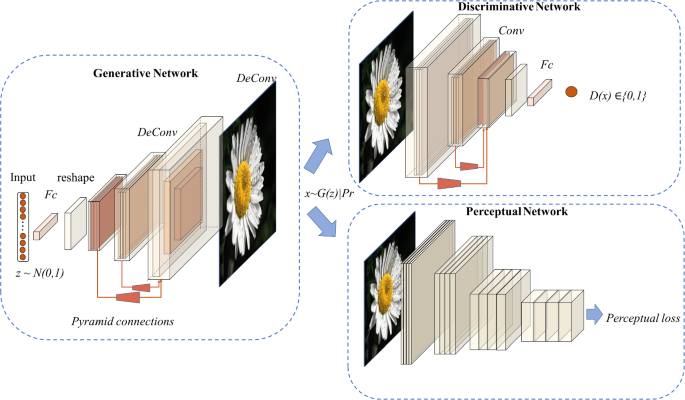
The overall structure of SSGAN is illustrated in Fig. 1. The SSGAN model consists of three main components: the generative network, the discriminative network, and the perceptual network. The generative network is responsible for transforming an input random noise vector \(z\) into an image \(G\left(z\right)\) with the expectation of deceiving the discriminative network. The discriminative network serves as a binary classifier to distinguish between the generated images \(G\left(z\right)\) and the real images \({P}_{r}\). These two components engage in a game to drive the GAN towards achieving Nash equilibrium. Our novel contribution is the inclusion of a perception network, which is responsible for extracting high-dimensional semantic features from the input images and comparing their semantic similarity with the distribution of real images. This facilitates the generator network in producing superior outputs.
The generator primarily consists of stacked transpose convolutional layers and pyramid connections. Specifically, it includes one fully connected layer, four transpose convolutional layers, and two sets of pyramid connections. The generator takes a one-dimensional random noise vector \(z\), following a Gaussian distribution, as input and generates images of size 64 × 64 × 3 as output. The discriminator is mainly composed of stacked convolutional layers and pyramid connections. It comprises four convolutional layers, two sets of pyramid connections, and one fully connected layer. Conventional techniques such as ReLU [7] and LN [6] are used to prevent overfitting and gradient disappearance. The discriminator network takes RGB images as input and outputs binary classification results. The perceptual network is a substructure of the VGG-19 [21] network pre-trained on the ImageNet dataset. We fix its parameters and select the first 16 layers as our feature extraction network model. In the overall architecture of the model, our innovation lies in the design of a pyramid structure for the backbone network to accommodate small sample sizes in image datasets. We have also introduced the perceptual network, which serves as an image semantic feature extraction module.
3.2 Pyramid Connection
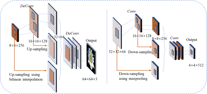
The function of the pyramid connection is to fuse feature maps of different scales through upsampling and downsampling operations in different ways. As the connected feature maps have sizes resembling a “pyramid” structure, we named it the pyramid connection. Figure 2 illustrates the details of the pyramid connection. In the figure, the generation network utilizes bilinear interpolation for upsampling, which, together with transposed convolution (Deconv), performs feature extraction and fusion operations in the model. This is because: (1) Using transpose convolution for upsampling, although it can increase the size of the feature maps and refine coarse feature maps, it often leads to the “checkerboard artifacts” due to uneven overlap of the convolution kernels. To address this issue, we introduce the pyramid connection and utilize upsampling with bilinear interpolation, which helps alleviate the problem of pixel discontinuity and mitigate the checkerboard effect. (2) Due to the varying expressive power of feature maps at different levels, shallow-level features primarily reflect details such as brightness, edges, while deep-level features capture overall structures and semantic information. The introduction of pyramid connections allows the model to integrate features from different dimensions, enhancing the feature extraction capability of the model. (3) Additionally, the introduction of pyramid connections provides the model with receptive fields different from those obtained by transpose convolution, further enhancing the model's performance.
3.3 Perceptual Loss
As shown in Fig. 1, we innovatively incorporate a perceptual network to extract high-dimensional feature maps. This network is based on a pre-trained VGG network with 16 layers, which exhibits strong generalization capabilities due to the rich species diversity in the ImageNet dataset. Based on this, we introduce the perceptual loss, which ensures high-dimensional semantic similarity between the generated samples and the original samples. The perceptual loss is defined as the Euclidean distance between the feature representations of the reconstructed images and the real images, as shown in Eq. 1.
Here \(W\) and \(H\) respectively represent the dimension of the output feature map within the VGG network, namely height and width.\(\phi \left(\widetilde{x}\right)\) represents the output characteristic matrix of the generated image in Perceptual Network, and \(\phi \left(x\right)\) represents the output characteristic matrix of the real image in Perceptual Network.
In particular, we combine the original critic loss calculated by Wasserstein distance with perceptual loss as our loss function to optimize the GAN model. Our new objective can be expressed as follows:
where \({p}_{noise}\) denotes normal distribution, \({p}_{r}\) represents real plant data distribution.\({P}_{g}\) represents the data distribution of the generated image.\({\mathbb{E}}\) represents mathematical expectation. \({p}_{\widehat{x}}\) is defined implicitly as sampling uniformly along straight lines between pairs of points sampled from \({p}_{r}\) and the generator distribution \(G\left({p}_{noise}\right)\). Enforcing the unit gradient norm constraint everywhere along these straight lines is sufficient. We train the discriminator and the generator by alternatively minimizing \({L}_{G}\) and \({L}_{D}\).
4 Experimental Setup
4.1 Experimental Environment
Our experiments are conducted on the graphics processing units (GPUs) of NVIDA GeForce RTX 3060Ti with 8 GB graphics memory size, 14 GHz memory clock, bit width is 256bit. In addition, the processor model of the computer is i7-12700 K, the memory size is 32 GB, and the operating system is Window 10. The model implementation is based on TensorFlow 2.0 framework, Integrated Development environment (IDE) is PyCharm. The main toolkits used are numpy, random, glob, imageio, math, time, os, etc. The main programming language used is Python 3.7.
4.2 Dataset
We conducted extensive experiments on two image datasets, “Flower” and “Animal”.
The “Flower” dataset consists of images of five different types of flowers: dandelions, sunflowers, tulips, daisies, and roses. Each category contains approximately 1000 images. It is worth noting that dandelions, daisies, and sunflowers belong to the family Asteraceae and share highly similar phenotypic features, which poses a challenge for our classification task.
The “Animal” dataset includes images of three animal categories: cats, dogs, and tigers, with 500 images per category. To facilitate the experiments, all images were resized to a uniform size of 64 × 64 pixels.
All the real images from the original dataset were included in the training of the GAN network. To evaluate the augmented effect of SSGAN, we also trained and tested the classifier using the augmented dataset.
The augmented dataset consists of 500 real images per category and 400 generated images per category. From each category, 100 randomly selected real images were used as the test set for the classifier, while the remaining data was used for training the classifier.
4.3 Hyperparameters
In contrast to other deep learning models, the training of a GAN requires iterative updates of the generator and discriminator, aiming to reach a Nash equilibrium state where both components have minimized their individual losses. Training is halted once the model reaches this equilibrium. At this stage, a lower loss value indicates superior model performance.
4.3.1 Learning Rate
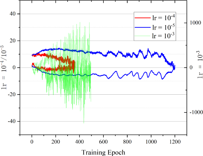
We conducted experiments with different learning rates, and observed that excessively large learning rates led to significant oscillations in the model's performance. As the learning rate decreased, the oscillations gradually diminished, but the convergence speed also slowed down. We present the results of three different learning rates 10–3, 10–4, and 10–5 to observe the model's training process, as shown in Fig. 3. Figure 3 illustrates that when the learning rate was set to 10–3, the model exhibited significant oscillations. In comparison, the model converged faster when the learning rate was set to 10–4 compared to 10–5. Consequently, we ultimately chose a learning rate of 10–4 for our model.
4.3.2 \({\varvec{\mu}}\)and \({\varvec{\lambda}}\)
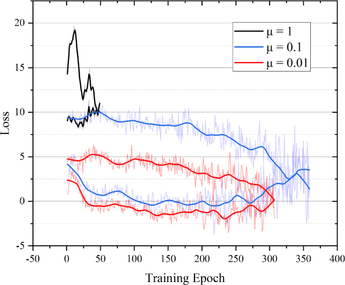
In the loss function, we varied the hyperparameter μ and evaluated the model's training process. The symbols μ and λ represent hyperparameters in Eqs. 2 and 3, where μ is a hyperparameter that controls the influence of the perceptual loss \({L}_{P}\) on the generator loss, and λ is a hyperparameter that controls the influence of the gradient penalty regularization term on the discriminator loss. Figure 4 illustrates the training results for different values of μ. Specifically, we tested μ with values of 1, 0.1, and 0.01. From the figure, it can be observed that when μ is set to 1, the model exhibits faster convergence but yields higher loss values. In contrast, when μ is set to 0.01, the model achieves faster convergence to the Nash equilibrium and demonstrates the lowest loss values compared to the case with μ set to 0.1.
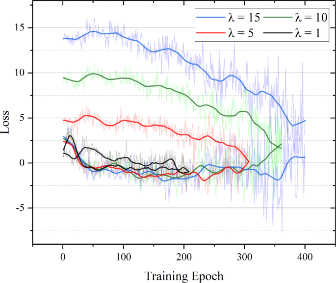
In our experiments, we varied the hyperparameter λ in the loss function and examined the model's training process. Figure 5 presents the training results for different values of λ. Specifically, we tested λ with values of 1, 5, 10, and 15. From the figure, it can be observed that when λ is set to 1, SSGAN achieves the minimum loss value at the Nash equilibrium. Consequently, based on this observation, we determined the optimal hyperparameter settings for our model as a learning rate of 10–4, μ value of 0.01, and λ value of 1.
4.4 Evaluation Metrics
4.4.1 Visualization of Generated Results
The real visual feedback of the generated image is important metrics to evaluate the ability of model generation. This evaluation method will generate images for visual output, and compare them to observe the clarity of texture details, image diversity and whether pattern collapse occurs.
4.4.2 t-SNE
t-SNE (t-Distributed Stochastic Neighbor Embedding) is a non-linear dimensionality reduction algorithm that is particularly suitable for reducing high-dimensional data to 2D or 3D while preserving the similarity in the joint probability distribution between the low-dimensional and original data. Let \({x}_{i}\) and \({x}_{j}\) represent points in the original space, and \({y}_{i}\) and \({y}_{j}\) represent their corresponding points in the low-dimensional space. The objective function \(Obj\) of t-SNE can be expressed as follows:
Here, \({p}_{ij}\) represents the Gaussian joint probability distribution between data points in the original data space, while \({q}_{ij}\) represents the corresponding joint probability distribution between points in the target space after dimensionality reduction. Specifically, \({q}_{ij}\) is computed using the Student’s t-distribution. The objective function, as defined in t-SNE, aims to minimize the Kullback–Leibler divergence between these two probability distributions, indicating the similarity between the distributions.
4.4.3 Objective Evaluation Metrics
Meanwhile, inception score (IS) and Fréchet inception distance (FID) are two other important indicators to measure the quality and diversity of the pictures generated by the GAN. IS evaluates the quality of the model from both image clarity and image diversity perspectives. But FID considers more the connection between the generated images and the real images. The larger the IS value, the smaller the FID value, and the better the expression effect. Their formulas for the calculation are as follows:
Time and space complexity are two basic metrics to measure the performance of network. This evaluation method separately calculates the number of parameters and the floating-point operations (i.e., FLOPs) to measure the complexity of the algorithm.
The smaller the spatiotemporal complexity metric, the less resources required for model training and the higher the model performance.
Parameter number
FLOPs
\({k}_{w}\times {k}_{h}\) represents the kernel size of the convolution layer; \({n}_{in}\) indicates the number of input channels and \({n}_{out}\) indicates the number of output channels. \(H\) and \(W\) represents the height and width of the output feature map.
4.4.4 Improvement in Classification Performance
In this evaluation method, ResNet-18 [11] is chosen as the classifier, and the augmented image set is used for the classification task. The validity of the model can be judged intuitively by comparing whether the classification accuracy and the precision are improved before and after the augmentation of the image set. The above metrics can be defined as follows.
\(TP\), \(TN\) and \(FN\) represent the samples belong to True Positive (TP), False Positive (FP), False Negative (FN), and True Negative (TN) of the category, respectively.
5 Results
5.1 Ablation Study
In this section, we conducted detailed ablation experiments to demonstrate the individual effects of the pyramid connection module and the perceptual loss component on the overall model.
5.1.1 Generated Image Visualization
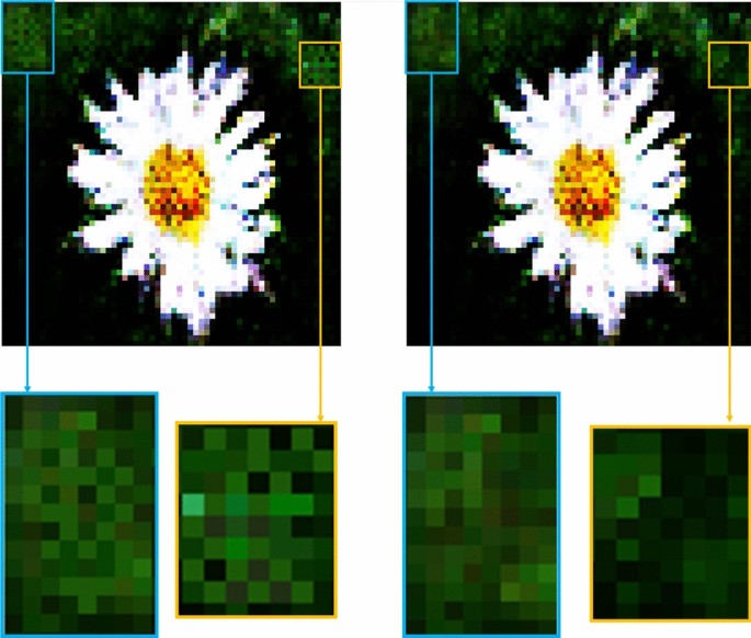
Checkerboard artifact refers to the grid-like pattern of varying color intensity that appears in generated images, resulting from uneven overlapping of deconvolution operations [20]. Figure 6 illustrates a comparison between the generated images of SSGAN before and after the introduction of pyramid connections. The left side of Fig. 6 shows the images generated by SSGAN without pyramid connections, while the right side shows the images generated by SSGAN with pyramid connections. It can be observed that the introduction of pyramid connections effectively alleviates the checkerboard artifacts.
5.1.2 Evaluation of Generated Image Quality and Diversity
Table 1 presents the FID and IS scores of SSGAN, SSGAN without Perceptual Loss (PL), SSGAN without Pyramid Connection (PC) and SSGAN without Pyramid Connection and perceptual loss. The IS score measures the clarity and diversity of generated images, where a higher score indicates better performance. On the other hand, the FID score reflects the distance between generated and real images, with a lower score indicating better similarity.
According to Table 1, the complete SSGAN achieved the best FID and IS scores, demonstrating that it generates images with the highest quality and diversity. The Perceptual Loss resulted in an FID reduction of 11 and an IS improvement of 1.58. The Pyramid Connection led to an FID reduction of 19.3 and an IS improvement of 1.7. The combination of perceptual loss and pyramid connections in SSGAN led to a decrease of 24.3 in FID and an increase of 2.17 in IS. This confirms the positive impact of both components in enhancing the overall performance of the model.
5.1.3 t-SNE Visualization
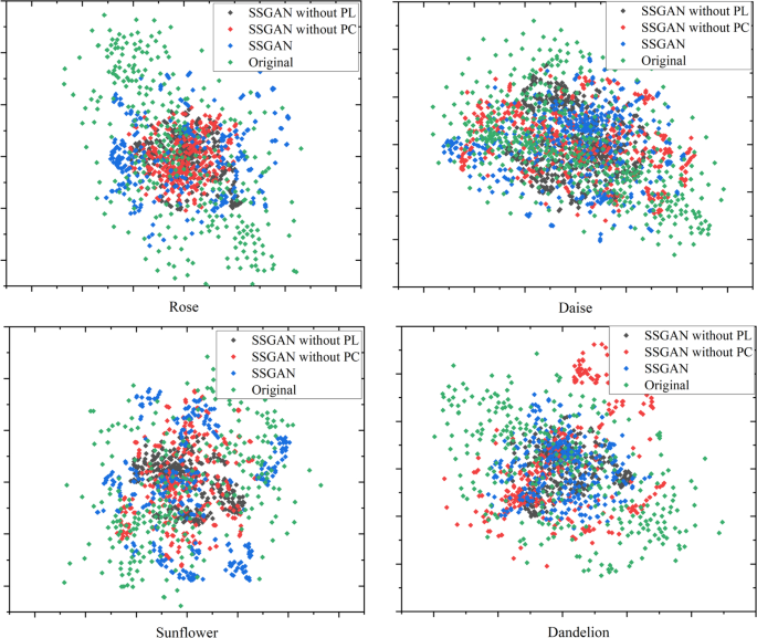
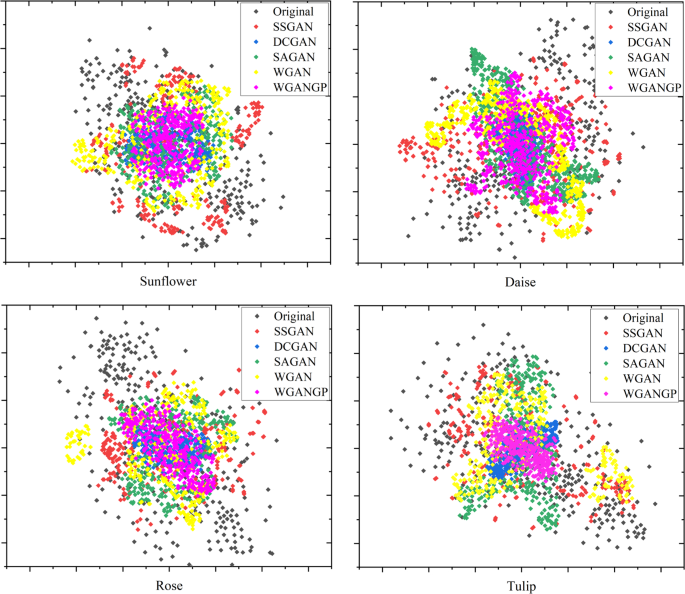
t-SNE is employed as a metric to assess the similarity between generated and original images in terms of their distribution. A well-clustered distribution of generated and original images in the t-SNE space indicates high-quality generated images. Moreover, if the generated images exhibit significant dispersion, it signifies a greater diversity in the generated image set. Figure 7 showcases the augmented results of several image classes in the “Flower” dataset.
It can be observed that the generated images by SSGAN exhibit the highest overlap with the real images and demonstrate good dispersion. The SSGAN without perceptual loss generates images with lower dispersion, indicating a lower diversity in the generated image set. Similarly, the SSGAN without pyramid connection generates images with comparatively lower dispersion compared to the SSGAN.
5.2 Comparison Experiment
In this section, we trained the proposed method along with several classic approaches such as WGAN, SAGAN, DCGAN, and WGAN-GP on a small-sample dataset. We compared the augmented effects among these methods and demonstrated the effectiveness of the proposed approach. The augmented effects among these methods were compared, and the effectiveness of the proposed approach was demonstrated.
5.2.1 Generated Image Visualization
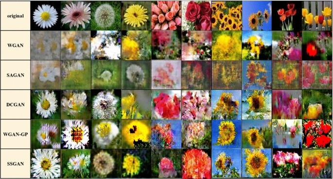
Figure 8 presents the generated images from several methods, providing an intuitive impression of their respective generation performances. It can be observed that SSGAN produces images with superior clarity, diversity, and finer details in terms of edges and textures compared to other methods. Following SSGAN, WGAN-GP and SAGAN exhibit relatively good generation results, while DCGAN and WGAN perform less favorably in generating high-quality images.
5.2.2 t-SNE Visualization
The distribution of generated images in t-SNE space can reflect the quality and diversity of the images. A higher degree of overlap between the distributions of generated and original images in t-SNE space indicates higher image quality. Additionally, if the distribution of generated images itself exhibits good dispersion in t-SNE visualization, it indicates better diversity of generated images.
Figure 9 displays the t-SNE visualization results of the generated images by various methods on the “Flower” dataset. It can be observed that compared to other methods, SSGAN exhibits better dispersion in the distribution, indicating superior diversity in the generated images. Additionally, the distribution of SSGAN shows the highest degree of overlap with the distribution of the original data, confirming the highest quality of the generated images.
5.2.3 Quantitative Evaluation
We compared the generation performance of our proposed SSGAN with six classical GANs on the “Flower” dataset, and the results are shown in Table 2, the optimal performance is highlighted in bold. Our SSGAN achieved state-of-the-art performance in terms of both FID and IS metrics. Specifically, the FID score decreased by 18.6 compared to the second-best method, and the IS score increased by 1.39 compared to the second-best method. This indicates that the images generated by SSGAN exhibit better clarity and diversity. Compared to other models, SSGAN has lower spatiotemporal complexity.
5.2.4 Classification Improvement
We utilized the augmented datasets to train the ResNet-18 [11] classifier and evaluated the improvement in classification performance. The training set of the augmented dataset consisted of two variations: 400 real images combined with 200 generated images, and 400 real images combined with 400 generated images. Table 3 presents the classification performance of the classifier trained on the augmented datasets using different methods, the optimal performance is highlighted in bold.
Our proposed SSGAN method demonstrates the best performance in enhancing the accuracy of downstream classification tasks. In both variations of the augmented datasets, it achieves state-of-the-art results in terms of Accuracy and Precision. Specifically, compared to the second-best method, SSGAN improves Accuracy by 2% and Precision by 2.3%.
5.3 Model Generalization
To demonstrate the generalization performance of our model, we applied several different methods to augment the “Animal” dataset and compared their generated results.
5.3.1 Generated Image Visualization
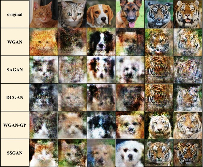
We randomly selected six images from each method’s generated image dataset for visualization, two images per class. The results are shown in the following figure.
Based on Fig. 10, it is evident that the images generated by SSGAN exhibit the best clarity and edge texture features. WGAN-GP follows closely in performance.
5.3.2 Quantitative Evaluation
Similarly, we performed sample augmentation using various GAN methods on the Animal dataset and compared the corresponding generated images based on their FID and IS results. Please refer to Table 4 for detailed information, the optimal performance is highlighted in bold.
According to Table 4, SSGAN also achieves state-of-the-art performance on the Animal dataset. Specifically, it exhibits a decrease of 6.6 in FID compared to the second-best method (WGAN-GP), and an increase of 3.2 in IS. This demonstrates the strong generalization capability of the proposed SSGAN method.
5.3.3 Classification improvement
We once again trained the ResNet-18 classifier using the augmented datasets generated by different methods and compared their performance. The results are shown in Table 5, the optimal performance is highlighted in bold.
According to Table 5, the classifier trained on the Animal dataset augmented by SSGAN achieved the best performance. It outperformed the second-best method, WGAN-GP, with improvements of 0.53% in Accuracy and 0.5% in Precision. The classifier’s overall performance on the Animal dataset was generally higher than on the Flower dataset. This can be attributed to the Animal dataset being a relatively simpler classification task. However, the performance improvement achieved through training on the augmented dataset was limited. This further demonstrates the good generalization performance of SSGAN.
5.4 Model Robustness
Robustness in deep learning refers to the model’s ability to maintain stability and effectiveness in the face of subtle modifications or perturbations to network parameters, as well as when input data is affected by noise (which may obscure critical information). Robustness evaluation is an important consideration to ensure that a model can maintain high performance when confronted with various data perturbations and noise. These approaches collectively contribute to evaluating the robustness of deep learning models:
Data Distribution Shift Assessment: In practical application scenarios, deep learning models may encounter data distributions that differ from those in their training data. Therefore, evaluating a model's robustness to data distribution shifts is of paramount importance. Our training data consists of noise that adheres to a normal distribution. To assess the model's performance across various distributions, we introduce noise conforming to different data distributions, such as Poisson distribution and random distribution, as input. This enables us to evaluate the model's performance under diverse distribution settings.
Noise and Interference Robustness Evaluation: Assessing the model’s robustness to various types of noise and interference is essential. Random noise can be added on top of the original input, and the model's performance change can be observed.
Sensitivity Analysis: Sensitivity analysis evaluates the model’s sensitivity to variations in input parameters. Analyzing the response of the model to small changes in input parameters helps understand the model's responsiveness to input variations. In SSGAN, we set hyperparameters μ and λ to 0.01 and 1, respectively. By perturbing the hyperparameter settings, the model's robustness can be assessed.
Based on the three aspects mentioned above, we conducted comparative experiments, and the experimental results are presented in Tables 6 and 7.
Table 6 presents the performance of SSGAN when different distributions are used as inputs. It can be observed that using different data distributions as inputs has minimal impact on the model's performance. Additionally, adding random noise on top of the training data distribution also has very little effect on the model's performance. This demonstrates the robustness of the model to data distribution shifts and noise interference.
Table 7 shows the performance of SSGAN with different hyperparameter settings. It can be observed that the further the hyperparameters are set from their optimal values, the faster the model's performance decreases. However, the model continues to function normally without any crashes. This demonstrates that the model maintains stability and effectiveness when facing minor modifications and perturbations in network parameters, highlighting its robustness.
6 Discussion and Conclusion
In real-world scenarios, the problem of small samples in image datasets is widely prevalent. This limitation hinders the accuracy of recognition tasks, particularly in applications based on deep learning techniques such as fault image detection, critical medical image diagnosis, and endangered species recognition. Small sample image augmentation techniques can augment the image dataset, thereby improving the accuracy of downstream image learning tasks. Thus, these techniques hold significant research value.
The paper proposes a novel image small sample augmentation method called SSGAN based on semantic similarity. The key innovations are as follows:
-
(1)
The design of a relatively shallow GAN backbone structure to adapt to small sample sizes. This allows the model to effectively learn from limited data.
-
(2)
The introduction of a pyramid connection structure to enhance the model's feature extraction capability and alleviate the checkerboard artifact issue.
-
(3)
The optimization of the loss function using an image high-dimensional semantic feature filtering module, which enhances the model’s learning ability by focusing on important semantic features.
These innovations collectively contribute to the effectiveness of the SSGAN method in addressing the challenges posed by small sample sizes in image augmentation tasks. We conducted extensive ablation and comparative experiments on the “Flower” dataset. The results of the experiments demonstrate that SSGAN achieves state-of-the-art performance in the task of small sample image enhancement. It outperforms the best-known methods by improving the FID and IS metrics by 18.6 and 1.4, respectively. The dataset enhanced by SSGAN contributes to achieving state-of-the-art performance in downstream classification tasks, with a 2.2% increase in accuracy compared to the best-known methods. In addition, transfer experiments were conducted on the 'Animal' dataset, and promising results were achieved, demonstrating the good generalization performance of the model. Through comparative experiments, we demonstrated that the model exhibits good robustness. Due to hardware limitations, we did not perform augmentation experiments on high-resolution images. In the future, we will continue to research methods for augmenting small sample high-resolution images.
References
Aljohani A, Alharbe N (2022) Generating synthetic images for healthcare with novel deep Pix2Pix GAN. Electronics 11
Arjovsky M, Chintala S, Bottou L (2017) Wasserstein generative adversarial networks. Int Conf Mach Learn 70:10
Boztas G (2023) Comparison of acoustic signal-based fault detection of mechanical faults in induction motors using image classification models. T I Meas Control 45:2794–2801
Carratino L, Cisse M, Jenatton R, Vert J (2022) On mixup regularization. J Mach Learn Res 23
Cheung T, Yeung D (2023) A survey of automated data augmentation for image classification: learning to compose, mix, and generate. IEEE T Neur Net Lear
Xu J, Sun X, Zhang Z, Zhao G, Lin J (2019) Understanding and improving layer normalization. Adv Neural Inf Process Syst 32
Dahl GE, Sainath TN, Hinton GE (2013) Improving deep neural networks for LVCSR using rectified linear units and dropout. In: 2013 IEEE international conference on acoustics, speech and signal processing, pp 8609–8613
Gulrajani I, Ahmed F, Arjovsky M, Dumoulin V, Courville A (2017) Improved training of Wasserstein GANs. Adv Neural Inf Process Syst 30:11
Isaksson LJ, Summers P, Raimondi S, Gandim S, Bhalerao A, Marvaso G, Petralia G, Pepa M, Jereczek-Fossa BA (2022) Mixup (sample pairing) can improve the performance of deep segmentation networKS. J Artif Intell Soft 12:29–39
Ishibashi H, Higa K, Furukawa T (2022) Multi-task manifold learning for small sample size datasets. Neurocomputing 473:20
Jian S, Kaiming H, Shaoqing R, Xiangyu Z (2016) Deep residual learning for image recognition. In: 2016 IEEE conference on computer vision and pattern recognition (CVPR), pp 770–778
Kang M, Shim W, Cho M, Park J (2021) Rebooting ACGAN: auxiliary classifier GANs with stable training. Adv Neural Inf Process Syst 34:14
Kim JY, Lee HE, Choi YH, Lee SJ, Jeon JS (2019) CNN-based diagnosis models for canineulce rative Keratitis. Sci Rep-UK 9:7
Kosolwattana T, Liu C, Hu R, Han S, Chen H, Lin Y (2023) A self-inspected adaptive SMOTE algorithm (SASMOTE) for highly imbalanced data classification in healthcare. Biodata Min 16:14
Odena A, Olah C, Shlens J (2017) Conditional image synthesis with auxiliary classifier GANs. Int Conf Mach Learn 70:10
Radford A, Metz L, Chintala S (2015) Unsupervised representation learning with deep convolutional generative adversarial networks. arXiv preprint arXiv:1511.06434
Ravindran P, Costa A, Soares R, Wiedenhoeft AC (2018) Classification of CITES-listed and other neotropical Meliaceae wood images using convolutional neural networks. Plant Methods 14:10
Sampath V, Maurtua I, Martin JJA, Iriondo A, Lluvia I, Aizpurua G (2023) Intraclass image augmentation for defect detection using generative adversarial neural networks. Sensors-Basel 23
Satterlee N, Torresani E, Olevsky E, Kang JSS (2023) Automatic detection and characterization of porosities in cross-section images of metal parts produced by binder jetting using machine learning and image augmentation. J Intell Manuf
Shi C, Zhang T, Liao D, Jin Z, Wang L (2022) Dual hybrid convolutional generative adversarial network for hyperspectral image classification. Int J Remote Sens 43:28
Simonyan K, Zisserman A (2014) Very deep convolutional networks for large-scale image recognition. In: 3rd international conference on learning representations (ICLR 2015). computational and biological learning society
Zhang H, Goodfellow I, Metaxas D, Odena A (2019) Self-attention generative adversarial networks. Int Conf Mach Learn 97(97):10
Le Z, Wei H, Lyu Z, Wei H, Li P (2021) A small-sample faulty line detection method based on generative adversarial networks. Expert Syst Appl 169:11
Zhang M, Zou F, Zheng J (2017) The linear transformation image enhancement algorithm based on HSV color space. Adv Intell Inf Hiding Multim Signal Process 2(64):19–27
Zhu Q, Mao Q, Jia H, Noi OEN, Tu J (2022) Convolutional relation network for facial expression recognition in the wild with few-shot learning. Expert Syst Appl 189:9
Author information
Authors and Affiliations
Contributions
CM: Conceptualization, Methodology, Software, Visualization, Writing—Original Draft. JM: Data curation, Validation. WG: Formal analysis, Resources, Supervision, Writing—review & editing. ST: Formal analysis, Investigation, Supervision, Writing—review & editing.
Corresponding author
Ethics declarations
Conflict of interest
The authors declare no competing interests.
Additional information
Publisher's Note
Springer Nature remains neutral with regard to jurisdictional claims in published maps and institutional affiliations.
Rights and permissions
Open Access This article is licensed under a Creative Commons Attribution 4.0 International License, which permits use, sharing, adaptation, distribution and reproduction in any medium or format, as long as you give appropriate credit to the original author(s) and the source, provide a link to the Creative Commons licence, and indicate if changes were made. The images or other third party material in this article are included in the article's Creative Commons licence, unless indicated otherwise in a credit line to the material. If material is not included in the article's Creative Commons licence and your intended use is not permitted by statutory regulation or exceeds the permitted use, you will need to obtain permission directly from the copyright holder. To view a copy of this licence, visit http://creativecommons.org/licenses/by/4.0/.
About this article
Cite this article
Ma, C., Mi, J., Gao, W. et al. SSGAN: A Semantic Similarity-Based GAN for Small-Sample Image Augmentation. Neural Process Lett 56, 149 (2024). https://doi.org/10.1007/s11063-024-11498-z
Accepted:
Published:
DOI: https://doi.org/10.1007/s11063-024-11498-z


