Comparison of numerical and computational aspects between two constraint-based contact methods in the description of wheel/rail contacts

Abstract

The numerical and computation aspects of the Knife-edge Equivalent Contact (KEC) constraint and lookup table (LUT) methods are compared in this paper. The LUT method implementation uses a penetration-based elastic contact model for the flange and a constraint-based formulation at the wheel tread. For the KEC method, where an infinitely narrow rail contacts an equivalent wheel, regularization of the tread-flange transition is adopted to simultaneously account for tread and flange contacts using constraints. A comparison between the two methods is carried out using well-known numerical integrators to show the applicability and limitations of both methods.

Two fixed-step-size integrators, the explicit Runge–Kutta (RK4) and the predictor–corrector Adam–Bashforth–Moulton (ABM) methods, and two variable-step-size Matlab built-in function integrators, the explicit $ode45$ and implicit $ode15s$, were applied to get the numerical solutions to the dynamic problems and study the relative numerical performance of the two contact description methods. To complete the railway vehicle model, both contact methods were implemented for the multibody model of a benchmark railway vehicle (the Manchester wagon 1). Numerical results were obtained for different railway tracks with and without irregularities. Profiles of the S1002 wheel and LB-140-Area rail, which demonstrate the two-point contact phenomenon, were considered. Both methods were implemented in Matlab and validated against commercial simulation software. The kinematic results for both approaches show good agreement, but the KEC method was up to 20% more efficient than the LUT method regardless of integrator used.

Nomenclature

$\mbox{$\textbf {A}$}^{t}$ :

Rotation matrix from a track frame with respect to the global frame

$\mbox{$\textbf {A}$}^{\mathit{bti}}$ :

Rotation matrix of the body track frame with respect to the global frame

$\mbox{$\textbf {A}$}^{\mathit{bti},i}$ :

Rotation matrix of body frame with respect to the body track frame

$\mbox{$\textbf {A}$}^{\mathit{wti},\mathit{wi}}$ :

Rotation matrix of wheelset frame with respect to the wheelset track frame

$\mbox{$\textbf {A}$}^{\mathit{wti},\mathit{wIi}}$ :

Rotation matrix of wheelset intermediate frame with respect to the wheelset track frame

$\mbox{$\textbf {A}$}^{\mathit{wIi},\mathit{wi}}$ :

Rotation matrix of wheelset frame with respect to the wheelset intermediate frame

$\mbox{$\textbf {A}$}^{t,\mathit{rp}}$ :

Rotation matrices of the rail profile frames with respect to the track frame

$\mbox{$\textbf {C}$}^{\mathit{LUT}}_{\mbox{$\textbf {q}$}}$ :

Jacobian matrix of LUT constraints

$\mbox{$\textbf {C}$}^{\mathit{LUT}}$ :

LUT constraint equations

$\mbox{$\textbf {C}$}^{\mathit{KEC}}$ :

KEC constraint equations

$D^{\mathit{damp}}$ :

Nonlinear damping constant for flange contact in LUT method [$\text{kN} \cdot\text{s}/\text{m}^{2}$]

$D$ :

Damping coefficient [kN⋅s/m]

$d$ :

Deformation length of the spring [m]

$\dot{d}$ :

Time derivative of spring deformation [m/s]

$f^{\mathit{susp}}$ :

Magnitude of the suspension force

$f^{\mathit{lk}}$ :

Value of the wheel equivalent profile

$f_{\mathit{klt}}^{k}$ :

KEC-lookup table of wheel equivalent profiles

$h^{r}$ :

Functions that define railhead profiles

$h^{w}$ :

Functions that define wheel profiles

$K$ :

Spring stiffness [kN/m]

$K^{\mathit{hertz}}$ :

Hertzian stiffness for flange contact in LUT method [$\text{N}/\text{m}^{1.5}$]

$K^{\mathit{series}}$ :

Damper series stiffness [kN/m]

$K^{\mathit{bend}}$ :

Bending stiffness [kN/rad]

$K^{\mathit{shear}}$ :

Shear stiffness [kN/m]

$l_{0}$ :

Undeformed spring length [m]

$L_{w}$ :

Wheel profile positioning with respect to the track centerline [m]

$L_{r}$ :

Rail profile positioning with respect to the track centerline [m]

$\mbox{$\textbf {M}$}$ :

Vehicle generalized mass matrix

$\mbox{$\textbf {N}$}$ :

Matrix that represents the direction of the reaction forces

$\bar{\mbox{$\textbf {n}$}}^{\mathit{wi}}_{c}$ :

Unit normal vector with respect to the wheel surface at the contact point

$\hat{\mbox{$\textbf {n}$}}_{c}^{\mathit{rp}}$ :

Unit normal vector with respect to the railhead surface at the contact point defined in rail profile frame

$\bar{\mbox{$\textbf {n}$}}_{c}^{\mathit{rp}}$ :

Unit normal vector of the contact point to the railhead surface defined in wheelset track frame

$\bar{\mbox{$\textbf {n}$}}_{c,\mathit{fla}}^{\mathit{rp}}$ :

Unit normal vector at flange contact point to the rail surface defined in wheelset track frame

$\mbox{$\textbf {q}$}$ :

Vector of multibody system coordinates

$\mbox{$\textbf {q}$}^{\mathit{wi}}$ :

Vector of relative wheelset track frame coordinates

$\mbox{$\textbf {Q}$}$ :

Vectors of generalized applied forces and generalized quadratic-velocity inertia forces

$\mbox{$\textbf {Q}$}^{\mathit{susp}}$ :

Vector of generalized suspension forces

$\mbox{$\textbf {Q}$}_{\mathit{fla}}^{\mathit{nor}}$ :

Vector of generalized wheel–rail normal flange forces

$\mbox{$\textbf {Q}$}^{\mathit{nor},\mathit{wi}},\ \mbox{$\textbf {Q}$}^{\mathit{nor},\mathit{wi}}_{\mathit{tre}},\ \mbox{$\textbf {Q}$}^{\mathit{nor},\mathit{wi}}_{\mathit{fla}}$ :

Vector of generalized wheel–rail normal contact forces, generalized wheel–rail normal contact forces at tread and flange

$\mbox{$\textbf {Q}$}^{\mathit{tang}}$ :

Vector of generalized tangential tread and flange forces

$R$ :

Radius of curved track [m]

$\mbox{$\textbf {R}$}^{t}$ :

Position vector of a track frame with respect to the global frame

$R^{t}_{x},\ R^{t}_{y},\ R^{t}_{z}$ :

Position components of the position vector $\mbox{$\textbf {R}$}^{t}$ in $X$, $Y$, and $Z$ direction

$\mbox{$\textbf {R}$}^{\mathit{bti}}$ :

Position vector of the body track frame with respect to the global frame

$\mbox{$\textbf {R}$}^{\mathit{ijt}}$ :

Relative distance vector from body track frames $\mathit{it}$ to $\mathit{jt}$

$\mbox{$\textbf {R}$}_{P}$ :

Absolute position vector of an point $P$ in global frame

$\bar{\mbox{$\textbf {r}$}}^{\mathit{ir}}$ :

Position vectors of rail irregularity vectors of rail profile frames with respect to ideal rail profile frames

$\bar{\mbox{$\textbf {r}$}}^{\mathit{rp}}$ :

Position vectors of ideal railhead frames with respect to track frame

$\mbox{$\textbf {r}$}_{P}^{i}$ :

Position vector of point $P$ that belongs to body $i$ with respect to the global frame

$\bar{\mbox{$\textbf {r}$}}^{i}$ :

Position vector of body frame with respect to its the body track frame

$\bar{\mbox{$\textbf {r}$}}^{\mathit{wi}}$ :

Position vector of wheelset frame with respect to the wheelset track frame

$\bar{\mbox{$\textbf {r}$}}_{c}^{\mathit{wi}}$ :

Position vectors of contact points with respect to the wheelset track frame

$\dot{\bar{\mbox{$\textbf {r}$}}}_{c}^{\mathit{wi}}$ :

Time derivative of the position vector $\bar{\mbox{$\textbf {r}$}}_{c}^{\mathit{wi}}$

$\bar{\mbox{$\textbf {r}$}}_{c,\mathit{fla}}^{\mathit{wi}}$ :

Position vectors of flange contact points with respect to the wheelset track frame

$\bar{\mbox{$\textbf {r}$}}_{c}^{\mathit{rp}}$ :

Position vectors of contact points with respect to the track frame

$\dot{\bar{\mbox{$\textbf {r}$}}}_{c}^{\mathit{rp}}$ :

Time derivative of the position vector $\bar{\mbox{$\textbf {r}$}}_{c}^{\mathit{rp}}$

$\bar{\mbox{$\textbf {r}$}}_{c,\mathit{fla}}^{\mathit{rp}}$ :

Position vectors of flange contact points with respect to the track frame

$r_{0}$ :

Rolling radius of the wheel when centered in the track [m]

$\mbox{$\textbf {s}$}$ :

Vector of wheel and rail surface parameters

$\mbox{$\textbf {s}$}_{\mathit{fla}}$ :

Vector of flange surface parameters

$s$ :

Arc-length associated with the track centerline [m]

$\Delta s$ :

Increment of the arc-length [m]

$\Delta\hat{s},\ \Delta\bar{s}$ :

Increment of the transition lengths of the regularization for the tread–flange transition [mm]

$s^{\mathit{wi}}$ :

Arc-length associated with the wheelset track centerline [m]

${s}^{w}_{1}$ :

Transverse wheel surface parameter [m]

${s}^{w}_{2}$ :

Angular wheel surface parameter [m]

${s}^{r}_{1}$ :

Longitudinal rail surface parameter [m]

${s}^{r}_{2}$ :

Transverse rail surface parameter [m]

${s}^{w}_{\mathit{fla}}$, ${s}^{r}_{\mathit{fla}}$:

Transverse wheel surface and rail surface parameters associated with flange contact [m]

$s^{k}$ :

Lateral positions of the contact point in the KEC-equivalent profiles [m]

$s_{\mathit{clt}}^{w}$, $s_{\mathit{clt}}^{r}$:

Contact lookup table of wheel and rail surface parameters [m]

$s_{\mathit{klt}}^{w}$, $s_{\mathit{klt}}^{r}$:

KEC-lookup table of wheel and rail surface parameters [m]

$\hat{\mbox{$\textbf {t}$}}_{c}^{\mathit{wIi}}$ :

Unit tangential vector with respect to the wheel surface at the contact point

$\bar{\mbox{$\textbf {t}$}}^{\mathit{wi}}_{c}$ :

Unit tangential vector defined in wheelset track frame

$\bar{\mbox{$\textbf {t}$}}^{\mathit{wi}}_{c,\mathit{fla}}$ :

Unit tangential vector for flange contact point defined in wheelset track frame

$\hat{\mbox{$\textbf {u}$}}_{P}^{i}$ :

Position vector of point $P$ with respect to body frame for body $i$ in the body frame

$\hat{\mbox{$\textbf {u}$}}^{\mathit{wIi}}_{c}$ :

Position vectors of the contact points at left and right wheel with respect to the wheelset intermediate frame

$\hat{\mbox{$\textbf {u}$}}^{\mathit{rp}}_{c}$ :

Position vectors of contact points with respect to rail profile frames

$V$ :

Forward velocity [m/s]

${y}^{\mathit{ir}}$ :

Position components of rail irregularity in lateral direction

$y^{\mathit{wi}}$ :

Lateral displacement of the wheelset frame with respect to the wheel track frame (ideal track centerline)

$\bar{y}^{\mathit{wi}}$ :

Lateral displacement of the wheelset frame with respect to the irregular track centerline

$y^{\mathit{wi}}_{\max}$, $y^{\mathit{wi}}_{\min}$:

Maximum and minimum values of the lateral displacements of wheelset

$\Delta y^{\mathit{wi}}$ :

Increment of the lateral displacements of wheelset

${z}^{\mathit{ir}}$ :

Position components of rail irregularity in vertical direction

$z^{\mathit{wi}}$ :

Vertical displacement of the wheelset frame with respect to the wheel track frame

$\bar{z}^{\mathit{wi}}$ :

Vertical displacement of the wheelset frame with respect to the irregular track centerline

$z_{\mathit{clt}}$ :

Contact lookup table of wheelset vertical displacement

$\boldsymbol{\lambda}$ :

Array of Lagrange multipliers

$\beta$ :

Orientation angle of the rail profiles

$\delta$ :

Linearized rotation angle due to the irregularity

$\delta^{\mathit{wi}},\ \dot{\delta}^{\mathit{wi}}$ :

Wheel–rail penetration at the flange contact and its rate

$\varphi^{t},\ \theta^{t},\ \psi^{t}$ :

Euler angles which define the orientation of track centerline with respect to global frame

$\varphi^{\mathit{wi}},\ \theta^{\mathit{wi}},\ \psi ^{\mathit{wi}}$ :

Euler angles which define the orientation of relative wheel frame with respect to wheelset track frame

$\bar{\varphi}^{\mathit{wi}}$ :

Roll angle of the wheelset frame with respect to the irregular track centerline

$\varphi_{\mathit{clt}}$ :

Contact lookup table of wheelset roll angle

$\mu$ :

Coefficient of friction

$\xi_{a}$ :

Alignment of the railhead centerlines’ irregularities [mm]

$\xi_{c}$ :

Cross level of the railhead centerlines’ irregularities [mm]

$\xi_{g}$ :

Gauge variation of the railhead centerlines’ irregularities [mm]

$\xi_{g,\max},\ \xi_{g,\min}$ :

Maximum and minimum values of the gauge variation the railhead centerlines’ irregularities [mm]

$\Delta\xi_{g}$ :

Increment of the gauge variation [mm]

$\xi_{v}$ :

Vertical profile of the railhead centerlines’ irregularities [mm]

$\langle O; X, Y, Z \rangle$ :

Global frame

$\langle O^{t}; X^{t}, Y^{t}, Z^{t} \rangle$ :

Track frame

$\langle O^{i}; X^{i}, Y^{i}, Z^{i} \rangle$ :

Body frame

$\langle O^{\mathit{lrp}}; X^{\mathit{lrp}}, Y^{\mathit {lrp}}, Z^{\mathit{lrp}} \rangle$ :

Left rail profile frame

$\langle O^{\mathit{rrp}}; X^{\mathit{rrp}}, Y^{\mathit {rrp}}, Z^{\mathit{rrp}} \rangle$ :

Right rail profile frame

$\langle O^{\mathit{bti}}; X^{\mathit{bti}}, Y^{\mathit {bti}}, Z^{\mathit{bti}} \rangle$ :

Body track frame for body $i$

$\langle O^{\mathit{wi}}; X^{\mathit{wi}}, Y^{\mathit{wi}}, Z^{\mathit{wi}} \rangle$ :

Wheelset frame

$\langle O^{\mathit{wIi}}; X^{\mathit{wIi}}, Y^{\mathit {wIi}}, Z^{\mathit{wIi}} \rangle$ :

Wheelset intermediate frame

1 Introduction

A railway vehicle is a complex mechanical system that consists of a large number of bodies, wheel/rail contacts, and complicated suspension elements. Because of the high computational loads, the real-time simulation of the railway vehicle is challenging [1], especially with respect to the wheel–rail contact [2]. Computationally efficient and physically accurate simulations can be used for a wide variety of applications, such as optimization problems and embedded models. Moreover, to analyze the validity and efficiency of different numerical methods, benchmark problems can be found in the literature. Examples include the Manchester benchmark [3] and the switches and crossings benchmarks [4].

In computational railway dynamics, a number of formalisms have been introduced to analyze wheel/rail contact. Among these, two well-known approaches are commonly used in multibody railway simulations. The first is the elastic approach [5–7], where interpenetration between wheel/rail surfaces is allowed, and normal contact forces are computed based on interpenetration and Hertzian parameters. However, the large magnitude Hertzian parameters that come about when applying the elastic approach can result in a stiff system of ordinary differential equations. Therefore, implicit integrators with small time steps are used, which increases computational cost. In [8], Liu and Bruni compared Hertzian and non-Hertzian wheel/rail contact models for multibody simulation. In [6], the Hertzian and non-Hertzian models are studied and compared to give the insight of proper selection of the parameters for better computational accuracy and efficiency. The second approach is the constraint method, which is also called Lagrange multiplier method. In this approach, the contact between wheel and rail is described with a set of kinematic constraint equations [9] to ensure both surfaces are in contact without penetration or separation. In this way, the normal contact forces can be computed using the Lagrange multipliers that are associated with the constraint equations.

Two constraint-based formulations for the wheel/rail contact in a multibody simulation have been studied here. The first is the LUT method. The LUT method is an offline constraint approach where the contact detection part of the analysis is carried out in a preprocessing stage and the solution is stored in a lookup table. In the subsequent dynamic simulations, the contact points are obtained by interpolating between the stored data points [10–12]. In the work of [10], an offline contact lookup table is used to predict tread contact point and an online elastic approach is used to predict flange contact. This algorithm was later extended to cover the combination of nodal and nonconformal contact detection to solve contact point jumps that can occur in turnouts [11]. The authors of [12] propose a constraint contact LUT method that accounts for track irregularities with two entries, lateral displacement, and track gauge variation. Using the Kalker book of tables for non-Hertzian contact (KBTNH) to build the lookup table is proposed [13] to generate the fast creep force. In that study, a regularization of the nonelliptical contact patch is introduced to solve the wheel/rail normal contact problem with non-Hertzian methods. In addition, the KBTNH is extended to include the full symmetry relations for creep forces and moment [14]. A comprehensive analysis to improve accuracy and efficiency when interpolating the lookup tables with multiple input parameters is presented in [15].

The second approach is the KEC method. The KEC method used here is an online constraint approach that was first proposed [16] to model wheel/rail contact. In the KEC method, the wheel/rail profile combination (see Fig. 1(a)) is established using an equivalent wheel profile (see solid lines in Fig. 1(b)) in contact with an infinitely narrow rail, which yields the equivalent allowable relative motion. This equivalent profile combination produces the same wheel/rail contact kinematics as the real wheel/rail profiles. As shown in Fig. 1(b), the contact points for a set of discrete values of the wheelset lateral displacement are located at the real wheel/rail profiles (dotted–dashed lines in Fig. 1(b)). The wheelset with wheels S1002 profile and rails LB.140-AREA profile are considered in the figure, and the geometry parameters for both wheel/ rail profiles are listed in Table 1. Accordingly, the corresponding contact points can be found on the KEC-equivalent profiles. See the solid lines in Fig. 1(b). The exact position of the contact points can be determined from the online solution of the KEC constraints. In addition, [17] proposed a regularization method to apply a continuous transition from tread to flange between each wheel/rail pair for the dynamic simulation of a two-point contact scenario. This regularization method can help avoid the finite contact point jumps that occur between tread and flange.

Fig. 1

(a) Real S1002 wheel profile and LB.140-AREA rail profile geometry, (b) contact points on real wheel/rail profiles and corresponding KEC-equivalent wheel/rail profiles, the real wheel/rail profiles correspond to the profiles in the dashed boxes on the left

Table 1 Parameters for the wheel/rail profile combination that illustrate the two-point contact scenario

Active research to develop computationally efficient models for multibody simulation of railroad vehicles is ongoing. Focus areas include linearizing the equations of motion [18], establishing an appropriate time integration method [18], efficiently detecting wheel/rail contact, and formalizing corresponding contact computation [10, 19, 20]. An explicit predictor–corrector integration method has been developed to solve the large-scale coupling dynamics of a railway vehicle and track system using the explicit method as the predictor and the implicit Newmark method as a corrector [21]. A quasielastic contact model proposed in [19] employs a two-dimensional spline approximation of contact solutions and stores the spline coefficients as a table in a pre–processing stage. The method is implemented in the wheel/rail module of the commercial software SIMPACK. In addition, a modal substructuring approach is proposed in [22] to improve the computational efficiency of a vehicle–track simulation by using a reduced number of modal coordinates. A hybrid contact detection algorithm is developed in [10] to eliminate the online iterative search for the second contact point. Moreover, a differential contact model is presented in [20] to reduce the computation cost by integrating the differential modeling of the wheel/rail contact problem with multibody modeling of the railway dynamics. The work reported in [18] proves that a simplified model based on weakly coupled lateral and vertical dynamics solves about four times faster than the full three-dimensional (3D) coupled dynamic model.

Several works have been published to study the pros and cons of the LUT and KEC methods with respect to computational efficiency. In the case of vehicle ML95 (Lisbon subway company) negotiating a curved track without irregularities in [12], a numerical solution is reached six times faster using the LUT method instead of directly applying contact constraints using the Matlab integrator $ode45$, $ode113$, and $ode4$. The authors of [16] conclude that the KEC method reduces computational cost up to $20\%$ compared to the LUT method using Matlab implicit integrator $ode15s$. And in [17], the KEC method proved to be 12.6 times more efficient than the 3D elastic contact simulation with the Matlab implicit integrator $ode15s$. Expanding on this preceding research, the objective of this work is to study the numerical and computational aspects of both methods using the multibody model of the Manchester wagon 1 proposed in [3]. Since efficient and stable time integration is a key issue [23] for the computational multibody dynamics of railroad vehicles, different well-known numerical integrators have been studied and compared in this paper. Two fixed-step-size integrators, RK4 and a predictor–corrector based ABM, and two variable-step-size Matlab integrators, $ode15s$ and $ode45$, are applied to solve railway dynamic problems. This will reveal numerical and computational aspects of the constraint-based contact approaches and will look at ways an accurate physics-based wheel/rail vehicle system could be analyzed in real-time.

The following Sect. 2 of this paper briefly introduces the multibody modeling of railway vehicles. Computer simulation of railway vehicles is presented in Sect. 3. Different integration methods are briefly introduced in Sect. 4. Sect. 5 compares the kinematics solutions of the modeled Manchester Wagon 1 with those obtained using standard commercial software and investigates the numerical and computational aspects of the KEC and LUT methods in detail. Finally, Sect. 6 provides a summary and offers conclusions.

2 Multibody modeling of railway vehicles

This section introduces details of the multibody modeling of railway vehicles. To this end, track kinematics vehicle kinematics and wheel/rail contact will be discussed. More insight into the kinematics and contact mechanism can be found in [12, 16, 24].

2.1 Track geometry and kinematics

In the multibody simulation of railway vehicles, the use of moving coordinate systems that follow the vehicles motion along the track centerline has been widely used in the literature [25, 26]. This method has advantages in the interpretation of the results because system coordinates are referred to track geometry. This work uses the so-called ‘track frame’ $\langle O^{t}; X^{t}, Y^{t}, Z^{t} \rangle$ for each vehicle body. The ‘track frame is defined along the track centerline and has the $X^{t}$ axis parallel to the tangential line of the track centerline, the $Y^{t}$ axis connecting the centerline of the two rails and the $Z^{t}$ axis perpendicular to the plane of the rails. See Fig. 2.

Fig. 2

Kinematics of the bodies $i$ and $j$ of a railway vehicle with relative body track frame coordinates, vectors $\mbox{$\textbf {R}$}^{\mathit{bti}}$ and $\mbox{$\textbf {R}$}^{\mathit{btj}}$ are the absolute position vectors of body track frames $\langle O^{t}; X^{t}, Y^{t}, Z^{t} \rangle$ with respect to global frame $\langle O; X, Y, Z \rangle$, $\bar{\mbox{$\textbf {r}$}}^{i}$ and $\bar{\mbox{$\textbf {r}$}}^{j}$ are position vectors of body $i$ and $j$ with their track frames

The absolute position vector and rotation matrix from a track frame to the global frame can be expressed as the functions of the arc-length $s$ as follows:

$$ \begin{aligned} & \mbox{$\textbf {R}$}^{t}(s) = \begin{bmatrix} R^{t}_{x}(s) \\ R^{t}_{y}(s) \\ R^{t}_{z}(s) \end{bmatrix} , \\ &\mbox{$\textbf {A}$}^{t}(s) = {\fontsize{7}{7}\selectfont \begin{aligned}[b] \begin{bmatrix} \cos(\theta^{t})\cos{(\psi^{t})} &\sin(\varphi^{t})\sin( \theta^{t})\cos{(\psi^{t})} -\cos(\varphi^{t})\sin{(\psi^{t})} & \sin(\varphi^{t})\sin{(\psi^{t})}+\cos(\varphi^{t})\sin(\theta^{t}) \cos{(\psi^{t})} \\ \cos(\theta^{t})\sin{(\psi^{t})} & \cos(\varphi^{t})\cos{(\psi^{t})}+ \sin(\varphi^{t})\sin(\theta^{t})\sin{(\psi^{t})}& \cos( \varphi^{t})\sin(\theta^{t})\sin{(\psi^{t})}-\sin(\varphi^{t}) \cos{(\psi^{t})} \\ -\sin(\theta^{t}) & \sin(\varphi^{t}) \cos(\theta^{t}) & \cos( \varphi^{t})\cos(\theta^{t}) \\ \end{bmatrix} \end{aligned} }, \end{aligned} $$

(1)

where $R^{t}_{x}$, $R^{t}_{y}$, $R^{t}_{z}$ are the components of the position vectors in the $X$, $Y$, and $Z$ direction, $\psi^{t}$ ($\mathit {azimut}$ or $\mathit{heading}$ angle), $\theta^{t}$ (vertical slope, positive when downwards in the forward direction), and $\varphi^{t}$ ($\mathit{cant}$ or $\mathit{superelevation}$ angle) are Euler angles which define the track centerline orientation.

With the description of the track frame, the geometry of the left and right rails centerlines can be obtained by defining two additional profile frames (left rail profile frame $\langle O^{\mathit{lrp}}; X^{\mathit{lrp}}, Y^{\mathit{lrp}}, Z^{\mathit{lrp}} \rangle$ and right rail profile frame $\langle O^{\mathit{rrp}}; X^{\mathit{rrp}}, Y^{\mathit{rrp}}, Z^{\mathit{rrp}} \rangle$) at the railheads. Both rail profiles are separated a distance $2L_{r}$ and rotated an angle $\beta$ in the ideal track configuration, as it is shown in Fig. 3. In addition, this ideal geometry description allows a straightforward definition of the irregular track by means of the left and right irregularity vectors $\bar{\mbox{$\textbf {r}$}}^{\mathit{lir}}$ and $\bar{\mbox{$\textbf {r}$}}^{\mathit {rir}}$ and the linearized irregularity angle $\delta$ defined as $\delta =(z^{\mathit{lir}}-z^{\mathit{rir}})/2L_{r}$. See Fig. 3. Note that the components of the irregularity vectors can be extracted from the following well-known centerlines’ irregularities measured in the railway industry:

Fig. 3

Description of track irregularity geometry: $\bar{\mbox{$\textbf {r}$}}^{\mathit{lrp}}$ and $\bar{\mbox{$\textbf {r}$}}^{\mathit {rrp}}$ are position vectors of ideal left and right railhead frames with respect to track frame, $\bar{\mbox{$\textbf {r}$}}^{\mathit{lir}}$ and $\bar{\mbox{$\textbf {r}$}}^{\mathit {rir}}$ are irregular vectors of left and right rail heads, $\hat{\mbox{$\textbf {u}$}}^{\mathit {lrp}}_{\mathit{lc}}$ and $\hat{\mbox{$\textbf {u}$}}^{\mathit{rrp}}_{\mathit{rc}}$ are position vectors of contact points with respect to rail profile frames, $\beta$ is the orientation angle of the rail profiles, $\delta$ is the linearized rotation angle due to the irregularity, and $L_{r}$ is the rail profile positioning with respect to the track centerline

• $\text{Alignment}~(\xi_{a})$	$\xi _{a}(s)=(y^{\mathit{lir}}+y^{\mathit{rir}})/2$,
• $\text{Vertical profile}~(\xi_{v})$	$\xi _{v}(s)=(z^{\mathit{lir}}+z^{\mathit{rir}})/2$,
• $\text{Gauge variation}~(\xi_{g})$	$\xi _{g}(s)=y^{\mathit{lir}}-y^{\mathit{rir}}$,
• $\text{Cross level}~(\xi_{c})$	$\xi _{c}(s)=z^{\mathit{lir}}-z^{\mathit{rir}}$.

All of these components can be implemented in a track preprocessor subroutine to parameterize the three-dimensional (3D) ideal track centerline and track irregularities as continuous functions (cubic splines in this work) of the longitudinal arc-length trajectory coordinate $s$. A schematic representation of the procedure used for the track preprocessor is presented in Fig. 4.

Fig. 4

Procedure of building track preprocessor

In this work, the track preprocessor for track centerline is discretized with constant step $\Delta s = 0.5\text{ m}$, which results in a Matlab storage size of around 200 kB (matrix size $2000\times7$) for 1000 m track. As for track irregularities, the track preprocessor is discretized with $\Delta s = 0.1\text{ m}$, which results in a Matlab storage size of around 300 kB (matrix size $10000\times5$) for 1000 m track.

2.2 Wheel/rail contact

As shown in Fig. 2, a body track frame $\langle O^{\mathit{ti}}; X^{\mathit{ti}}, Y^{\mathit{ti}}, Z^{\mathit{ti}} \rangle$ can be associated with body $i$ at any time-instant, when a body moves along the track with arc length $s^{i}$. Therefore, the position and orientation of the body track frame can be computed according to Eq. (1), as:

$$ \mbox{$\textbf {R}$}^{\mathit{ti}}=\mbox{$\textbf {R}$}^{t}(s^{i}), \quad \mbox{$\textbf {A}$}^{\mathit{ti}}=\mbox{$\textbf {A}$}^{t}(s^{i}). $$

(2)

Similarly, a wheelset track frame $\langle O^{\mathit{wti}}; X^{\mathit{wti}}, Y^{\mathit{wti}}, Z^{\mathit{wti}} \rangle$ is associated with the wheelset $i$ and with time. See Fig. 5. The position and orientation of the wheelset track frame can be calculated by replacing $s^{i}$ with $s^{\mathit{wi}}$ in Eq. (2).

Fig. 5

Frames for rigid wheelset kinematics: $\bar{\mbox{$\textbf {r}$}}^{\mathit{wi}}$ is the position vector of wheelset frame with respect to the wheelset track frame in the wheelset track frame, $\hat{\mbox{$\textbf {u}$}}^{\mathit{wIi}}_{\mathit{lc}}$ is the position vector of the left contact point at left wheel with respect to the wheelset intermediate frame

The set of relative wheelset track frame coordinates of a rigid wheelset $i$ (superscript $\mathit{wi}$) is given by:

$$ \mbox{$\textbf {q}$}^{\mathit{wi}} = \begin{bmatrix} s^{\mathit{wi}}&y^{\mathit{wi}}&z^{\mathit{wi}}& \varphi^{\mathit {wi}}& \theta^{\mathit{wi}}& \psi^{\mathit{wi}} \end{bmatrix} ^{T}, $$

(3)

where $y^{\mathit{wi}}$ is the lateral displacement and $z^{\mathit {wi}}$ is the vertical displacement of the wheelset frame with respect to the wheel track frame, respectively, and the $X$-component along the track centerline is zero; $\varphi^{\mathit{wi}}$, $\theta^{\mathit{wi}}$, and $\psi ^{\mathit{wi}}$ are Euler angles which define the orientation of relative wheel frame with respect to wheelset track frame.

The position vectors of right and left contact points, defined in the right and left railheads as shown in Fig. 3, are written with respect to wheelset track frame:

$$ \begin{aligned} & \bar{\mbox{$\textbf {r}$}}_{\mathit{rc}}^{\mathit{rrp}}=\bar {\mbox{$\textbf {r}$}}^{\mathit{rrp}}+ \bar{\mbox{$\textbf {r}$}}^{\mathit{rir}}+\mbox{$\textbf {A}$}^{t,\mathit{rrp}}\hat {\mbox{$\textbf {u}$}}_{\mathit{rc}}^{\mathit{rrp}}, \\ & \bar{\mbox{$\textbf {r}$}}_{\mathit{lc}}^{\mathit{lrp}}=\bar{\mbox{$\textbf {r}$}}^{\mathit{lrp}}+\bar{\mbox{$\textbf {r}$}}^{\mathit{lir}}+ \mbox{$\textbf {A}$}^{t,\mathit{lrp}}\hat{\mbox{$\textbf {u}$}}_{\mathit{lc}}^{\mathit{lrp}}, \end{aligned} $$

(4)

where $\mathit{lr}$ and $\mathit{rr}$ represent left rail and right rail, $\bar{\mbox{$\textbf {r}$}}^{\mathit{rrp}}$ and $\bar{\mbox{$\textbf {r}$}}^{\mathit{lrp}}$ are position vectors of ideal left and right railhead frames with respect to wheelset track frame, $\bar{\mbox{$\textbf {r}$}}^{\mathit{lir}}$ and $\bar{\mbox{$\textbf {r}$}}^{\mathit {rir}}$ are rail irregularity vectors of rail profile frames with respect to ideal left and right rail profile frames, $\mbox{$\textbf {A}$}^{t,\mathit{lrp}}$ and $\mbox{$\textbf {A}$}^{t,\mathit{rrp}}$ are rotation matrices from the railhead frames to the wheelset track frame, $\hat{\mbox{$\textbf {u}$}}_{\mathit{rc}}^{\mathit{rrp}}$ and $\hat{\mbox{$\textbf {u}$}}_{\mathit{lc}}^{\mathit{lrp}}$ contain the components of the position vector of contact points in the rail profile frames as shown in Fig. 3. The vectors and matrices are written as

$$ \begin{aligned} & \bar{\mbox{$\textbf {r}$}}^{\mathit{lrp}} = \begin{bmatrix} 0 \\ L_{r} \\ 0 \end{bmatrix} , \quad\quad\bar{\mbox{$\textbf {r}$}}^{\mathit{rrp}} = \begin{bmatrix} 0 \\ -L_{r} \\ 0 \end{bmatrix} ,\quad\quad\bar{\mbox{$\textbf {r}$}}^{\mathit{lir}}(s^{\mathit{wi}}) = \begin{bmatrix} 0 \\ y^{\mathit{lir}} \\ z^{\mathit{lir}} \end{bmatrix} ,\quad\quad\bar{\mbox{$\textbf {r}$}}^{\mathit{rir}}(s^{\mathit{wi}})= \begin{bmatrix} 0 \\ y^{\mathit{rir}} \\ z^{\mathit{rir}} \end{bmatrix} , \\ & \mbox{$\textbf {A}$}^{t,\mathit{lrp}}(s^{\mathit{wi}}) = \begin{bmatrix} 1 & 0 & 0 \\ 0 & \cos{(\beta+\delta)} & -\sin{(\beta+\delta)} \\ 0 & \sin{(\beta+\delta)} & \cos{(\beta+\delta)} \\ \end{bmatrix} , \quad \\ &\mbox{$\textbf {A}$}^{t,\mathit{rrp}}(s^{\mathit{wi}})= \begin{bmatrix} 1 & 0 & 0 \\ 0 & \cos{(-\beta+\delta)} & -\sin{(-\beta+\delta)} \\ 0 & \sin{(-\beta+\delta)} & \cos{(-\beta+\delta)} \\ \end{bmatrix} , \end{aligned} $$

(5)

The position vectors of contact points $\hat{\mbox{$\textbf {u}$}}_{\mathit {rc}}^{\mathit{rrp}}$ and $\hat{\mbox{$\textbf {u}$}}_{\mathit{lc}}^{\mathit{lrp}}$ in the rail profiles from Eq. (4) are parametrized according to the railhead profile geometry as shown in Fig. 6:

$$ \hat{\mbox{$\textbf {u}$}}^{\mathit{rrp}}_{\mathit{rc}}= \begin{bmatrix} 0 \\ {s}^{\mathit{rr}}_{2} \\ h^{\mathit{rr}}({s}^{\mathit{rr}}_{2}) \end{bmatrix} , \quad\hat{\mbox{$\textbf {u}$}}^{\mathit{lrp}}_{\mathit{lc}}= \begin{bmatrix} 0 \\ {s}^{\mathit{lr}}_{2} \\ h^{\mathit{lr}}({s}^{\mathit{lr}}_{2}) \end{bmatrix} , $$

(6)

where ${s}^{\mathit{lr}}_{2}$ and ${s}^{\mathit{rr}}_{2}$ are left and right transverse rail surface parameters, respectively, and $h^{\mathit{lr}}$ and $h^{\mathit{rr}}$ are the functions that define the railhead profiles.

Fig. 6

Wheel profile and rail profile geometry: $s_{1}^{w}$ and $s_{2}^{w}$ are transverse and angular wheel surface parameters, and $s_{1}^{r}$ and $s_{2}^{r}$ are longitudinal and transverse rail surface parameters, respectively

Also, special treatment is given to the railway vehicle wheelset bodies in a railway vehicle. An additional frame called ‘wheelset intermediate frame’ ($\mathit{wI}$) is defined as shown in Fig. 5. The $\mathit{wI}$-frame is defined as a body frame but shows no pitch rotation. As will be shown in the following section, it is a convenient frame to define contact point position vectors, because they are not influenced by the wheelset pitch rotation, which is particularly high in these bodies. More details about body and wheelset kinematics can be found in [12, 16, 24]. The position vector of contact points on the surface of the left and right wheel profile in Fig. 5 can be obtained in wheelset track frame, such as

$$ \begin{aligned} & \bar{\mbox{$\textbf {r}$}}_{\mathit{lc}}^{\mathit{wi}}= \bar {\mbox{$\textbf {r}$}}^{\mathit{wi}} + \mbox{$\textbf {A}$}^{\mathit{wti},\mathit{wIi}}\hat{\mbox{$\textbf {u}$}}_{\mathit {lc}}^{\mathit{wIi}}, \\ & \bar{\mbox{$\textbf {r}$}}_{\mathit{rc}}^{\mathit{wi}}= \bar{\mbox{$\textbf {r}$}}^{\mathit{wi}} +\mbox{$\textbf {A}$}^{\mathit{wti},\mathit{wIi}} \hat{\mbox{$\textbf {u}$}}_{\mathit{rc}}^{\mathit{wIi}}, \end{aligned} $$

(7)

where vector $\bar{\mbox{$\textbf {r}$}}^{\mathit{wi}}= \begin{bmatrix} 0& y^{\mathit{wi}}& z^{\mathit{wi}}\end{bmatrix} ^{T}$ is the position vector of the wheelset frame with respect to the wheelset track frame, $\hat{\mbox{$\textbf {u}$}}^{\mathit{wIi}}_{\mathit {lc}}$ and $\hat{\mbox{$\textbf {u}$}}^{\mathit{wIi}}_{\mathit{rc}}$ are the position vectors of the contact points at the left and right wheels with respect to the wheelset intermediate frame, and $\mbox{$\textbf {A}$}^{\mathit{wti},\mathit{wIi}}$ is the rotation matrix of the wheelset intermediate frame with respect to the wheelset track frame, which is given by the following equation:

$$ \mbox{$\textbf {A}$}^{\mathit{wti},\mathit{wi}} = \mbox{$\textbf {A}$}^{\mathit {wti},\mathit{wIi}}\mbox{$\textbf {A}$}^{\mathit{wIi},\mathit{wi}}, $$

(8)

where $\mbox{$\textbf {A}$}^{\mathit{wti},\mathit{wIi}}$ is the rotation matrix of the wheelset intermediate frame with respect to the wheelset track frame, $\mbox{$\textbf {A}$}^{\mathit{wIi},\mathit{wi}}$ is the rotation matrix of the wheelset frame with respect to the wheelset intermediate frame. These are given by

$$ \mbox{$\textbf {A}$}^{\mathit{wti},\mathit{wIi}} = \begin{bmatrix} 1 & - \psi^{\mathit{wi}} &0 \\ \psi^{\mathit{wi}} & 1& - \varphi^{\mathit{wi}} \\ 0 & \varphi^{\mathit{wi}} & 1 \end{bmatrix} , \quad \mbox{$\textbf {A}$}^{\mathit{wIi},\mathit{wi}} = \begin{bmatrix} \cos{( \theta^{\mathit{wi}})} &0 & \sin{( \theta^{\mathit{wi}})} \\ 0 & 1& 0 \\ -\sin{( \theta^{\mathit{wi}})} & 0 & \cos{( \theta^{\mathit{wi}})} \end{bmatrix} . $$

(9)

The position vectors of contact points $\hat{\mbox{$\textbf {u}$}}_{\mathit {rc}}^{\mathit{wIi}}$ and $\hat{\mbox{$\textbf {u}$}}_{\mathit{lc}}^{\mathit{wIi}}$ in the wheel profiles from Eq. (7) are parametrized according to the wheel profile geometry as shown in Fig. 6:

$$ \hat{\mbox{$\textbf {u}$}}^{\mathit{wIi}}_{\mathit{rc}}= \begin{bmatrix} h^{\mathit{rw}}({s}^{\mathit{rw}}_{1})\cos{({s}^{\mathit{rw}}_{2})} \\ -L_{w}+{s}^{\mathit{rw}}_{1} \\ -h^{\mathit{rw}}({s}^{\mathit{rw}}_{1})\sin{({s}^{\mathit{rw}}_{2})} \end{bmatrix} , \quad\hat{\mbox{$\textbf {u}$}}^{\mathit{wIi}}_{\mathit{lc}}= \begin{bmatrix} h^{\mathit{lw}}({s}^{\mathit{lw}}_{1})\cos{({s}^{\mathit{lw}}_{2})} \\ L_{w}+{s}^{\mathit{lw}}_{1} \\ -h^{\mathit{lw}}({s}^{\mathit{lw}}_{1})\sin{({s}^{\mathit{lw}}_{2})} \end{bmatrix} , $$

(10)

where $s_{1}^{w}$ and $s_{2}^{w}$ are the transverse and angular wheel surface parameters, respectively, and $h^{\mathit{lw}}$ and $h^{\mathit{rw}}$ are the functions that define the wheel profiles.

Based on the parameterization of the wheel and rail surfaces, contact can be modeled using the already defined elastic or constraint approach. For both approaches, 3D surface-to-surface contact can be reduced to a planar two-dimensional (2D) curve-to-curve contact assuming that the contact points lie in the $Y^{\mathit{wti}}$–$Z^{\mathit{wti}}$ plane of the wheelset track frame. This decreases the number of surface parameters from four to two, since the contact points at the left and right rails have the same arc-length parameter as the wheelset ($s_{1}^{r} = s^{\mathit{wi}}$), and the angular wheel parameters of the contact points are constant ($s_{2}^{w} = \pi/2$) in the $\mathit{wI}$-frame. Therefore, the simplified nomenclature ${s}^{w}={s}^{w}_{1}$ and ${s}^{r}={s}^{r}_{2}$ can be and is used in the rest of this paper. However, the main implication of this planar contact is that the wheelset yaw angle is neglected for the location of the contact points, which avoids the consideration of the so-called lead-lag contacts (flange contact points that are longitudinally displaced with respect to tread contacts). These contacts have an effect when the vehicle is negotiating very narrow curves, which usually occurs at very low velocities. Nevertheless, the planar contact approach is sufficiently accurate for most practical applications as shown in [12].

The use of 2D wheel/rail contact using the constraint approach is considered in the following. To this end, the following subsections briefly describe the basis of the following two planar constraint contact methods: contact lookup tables and the KEC method.

2.3 LUT method

Creation of constraint contact lookup table

The procedure to build a constraint contact lookup table starts by solving the contact constraints for different values of the wheelset relative position with respect to the track. The algorithm is summarized as follows:

• 1. Two sets of discrete numerical values are assigned to the lateral displacement of the wheelset $y^{\mathit{wi}}$ and gauge variation $\xi_{g}$:

  $$ \begin{aligned} & y^{\mathit{wi}} = y^{\mathit{wi}}_{\min}+\Delta y^{\mathit{wi}}, \quad y^{\mathit{wi}}\in[y^{\mathit{wi}}_{\min},~y^{\mathit {wi}}_{\max}],\\ & \xi_{g} = \xi_{g,\min}+\Delta\xi_{g}, \quad\xi_{g} \in[\xi _{g,\min},~\xi_{g,\max}], \end{aligned} $$

  (11)

  where $\Delta y^{\mathit{wi}}$ and $\Delta\xi_{g}$ are increments.

• 2. The wheelset coordinates $s^{\mathit{wi}}$, $\theta^{\mathit {wi}}$, and $\psi^{\mathit{wi}}$ are set to zero (contact points are assumed to lie in the $Y^{\mathit{wti}}$–$Z^{\mathit{wti}}$ plane of the wheelset track frame).

• 3. For a one-point contact scenario (when two wheel/tread contacts occur at both wheels), the six contact constraint equations of Eq. (12) are solved for different values of $y^{\mathit {wi}}$ and the nominal distance $2L_{r}^{*} = 2L_{r}+\xi_{g}$ in two for-loops to obtain six outputs: the wheelset kinematics $z^{\mathit {wi}}$, $\varphi^{\mathit{wi}}$, and the vector of tread surface parameters $\mbox{$\textbf {s}$}$,

  $$ \mbox{$\textbf {f}$}(z^{\mathit{wi}},\varphi^{\mathit{wi}},\mbox{$\textbf {s}$}) = \begin{bmatrix} \bar{\mbox{$\textbf {r}$}}^{\mathit{wi}}_{\mathit{lc}}-\bar{\mbox{$\textbf {r}$}}^{\mathit{lrp}}_{\mathit{lc}} \\ (\bar{\mbox{$\textbf {t}$}}^{\mathit{wi}}_{\mathit{lc}})^{T}\bar{\mbox{$\textbf {n}$}}_{\mathit{lc}}^{\mathit{lrp}} \\ \bar{\mbox{$\textbf {r}$}}^{\mathit{wi}}_{\mathit{rc}}-\bar{\mbox{$\textbf {r}$}}^{\mathit{rrp}}_{\mathit{rc}} \\ (\bar{\mbox{$\textbf {t}$}}^{\mathit{wi}}_{\mathit{rc}})^{T}\bar{\mbox{$\textbf {n}$}}_{\mathit{rc}}^{\mathit{rrp}} \\ \end{bmatrix} =\boldsymbol{0} ,$$

  (12)

  where $\mathit{rc}$ represents right wheel and $\mathit{lc}$ left wheel for one wheelset, $\mbox{$\textbf {s}$} = [s^{\mathit{lw}}\ \ s^{\mathit {lr}}\ \ s^{\mathit{rw}}\ \ s^{\mathit{rr}} ]^{T}$ is the vector of the surface parameters, $\bar{\mbox{$\textbf {t}$}}^{\mathit{wi}}_{c}$ is the unit tangential vector, and $\bar{\mbox{$\textbf {n}$}}_{c}^{\mathit{rp}}$ is the normal vector defined in the wheelset track frame, which can be expressed as follows:

  $$ \begin{aligned} & \bar{\mbox{$\textbf {t}$}}^{\mathit{wi}}_{c} = \mbox{$\textbf {A}$}^{\mathit{wti},\mathit{wIi}} \hat{\mbox{$\textbf {t}$}}_{c}^{\mathit{wIi}}, \\ & \bar{\mbox{$\textbf {n}$}}_{c}^{\mathit{rp}} = \mbox{$\textbf {A}$}^{t,\mathit {rp}}\hat{\mbox{$\textbf {n}$}}_{c}^{\mathit{rp}}, \end{aligned} $$

  (13)

  where $\hat{\mbox{$\textbf {t}$}}_{c}^{\mathit{wIi}}$ is the unit tangential vector with respect to the wheel surface at the contact point and $\hat{\mbox{$\textbf {n}$}}_{c}^{\mathit{rp}}$ is the unit normal vector with respect to the railhead surface at the contact point [16, 25]. In Eq. (12), given the value of lateral displacement $y^{\mathit{wi}}$, six contact constraints for one wheelset are solved to get six outputs: the wheelset coordinates $z^{\mathit{wi}}$ and $\varphi^{\mathit{wi}}$, and the surface parameters $\mbox{$\textbf {s}$}$ of the contact points at the tread.

• 4. The solution of Eq. (12) is stored in a lookup table with two entries. The lookup table defines the following functions:

  $$\begin{aligned} \begin{aligned} &{z}^{\mathit{wi}}= z_{\mathit{clt}}(y^{\mathit {wi}},\xi_{g}), \quad{\varphi}^{\mathit{wi}}= \varphi_{\mathit{clt}}(y^{\mathit{wi}},\xi_{g}), \\ &s^{\mathit{lw}}= s_{\mathit{clt}}^{\mathit{lw}}(y^{\mathit {wi}},\xi_{g}), \quad s^{\mathit{lr}}= s_{\mathit{clt}}^{\mathit {lr}}(y^{\mathit{wi}}, \xi_{g}), \quad s^{\mathit{rw}}= s_{\mathit{clt}}^{\mathit {rw}}(y^{\mathit{wi}},\xi_{g}), \quad s^{\mathit{rr}}= s_{\mathit {clt}}^{\mathit{rr}}(y^{\mathit{wi}}, \xi_{g}), \end{aligned} \end{aligned}$$

  (14)

  where $\mathit{clt}$ refers contact lookup table. Figure 7(a) shows the wheelset vertical displacement coordinate $z^{\mathit{wi}}$ with respect to the track centerline within a range of track gauge variations $\xi_{g}$ and Fig. 7(b) illustrates the contact lookup table.

  Fig. 7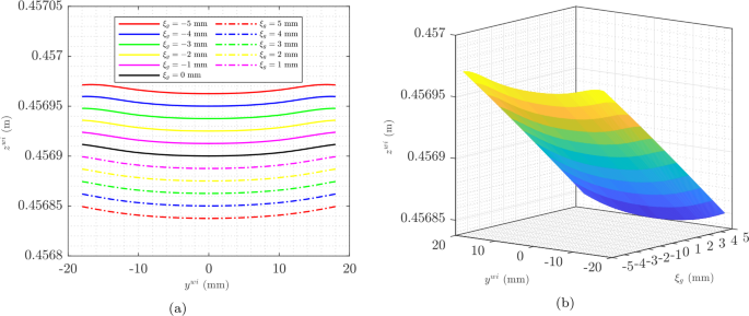

  

  (a) Wheelset vertical displacement with respect to track centerline for different values of gauge irregularity; (b) Contact lookup table for wheelset vertical displacement $z^{\mathit{wh}}$ with two entries. As it is observed, there is no wheel climbing due to the nature of the elastic flange contact used

Contact detection for two-point contact scenario

For the two-point contact scenario, contact detection at the flange is addressed using the maximum relative-indentation condition [5]. Therefore, two nonlinear equations are solved to obtain two flange surface parameters $\mbox{$\textbf {s}$}_{\mathit{fla}} = [s^{w}_{\mathit{fla}}\ \ s^{r}_{\mathit{fla}}]^{T}$ as follows:

$$ \mbox{$\textbf {f}$}(\mbox{$\textbf {s}$}_{\mathit{fla}}) = \begin{bmatrix} (\bar{\mbox{$\textbf {t}$}}^{\mathit{wi}}_{c,\mathit {fla}})^{T}( \bar{\mbox{$\textbf {r}$}}^{\mathit{wi}}_{c,\mathit{fla}}-\bar {\mbox{$\textbf {r}$}}^{\mathit{rp}}_{c,\mathit{fla}} ) \\ (\bar {\mbox{$\textbf {t}$}}^{\mathit{wi}}_{c,\mathit{fla}})^{T}\bar{\mbox{$\textbf {n}$}}_{c,\mathit{fla}}^{\mathit{rp}}\\ \end{bmatrix} =\boldsymbol{0} ,$$

(15)

where $\bar{\mbox{$\textbf {t}$}}_{c,\mathit{fla}}^{\mathit{wi}}$ and $\bar {\mbox{$\textbf {n}$}}_{c,\mathit{fla}}^{\mathit{rp}}$ are unit tangential and normal vectors, $\bar{\mbox{$\textbf {r}$}}^{\mathit{wi}}_{c,\mathit {fla}}$ and $\bar{\mbox{$\textbf {r}$}}^{\mathit{rp}}_{c,\mathit{fla}}$ are position vectors of the contact points on the wheel and railhead, all the above vectors are associated with the wheel–flange contact, and $c$ represents left contact $\mathit{lc}$ or right contact $\mathit {rc}$. Contact point detection at both the tread and flange for the LUT method is determined in a preprocessing stage that builds the contact lookup tables. During the dynamic simulations, the contact lookup table is used to interpolate the stored discrete data to get the contact point location.

Contact force computation for two-point contact scenario

For the LUT method, constraint contact is not appropriate when the number of contact points varies (i.e., from one contact point to the two-contact point scenario). For this reason, when flange contact occurs in the two-point contact scenario (before wheel climbing), a hybrid method is usually adopted [12]. In this approach, wheel/tread contact with the rail is considered using the constraint method and the wheel/flange contact with the rail is considered using the elastic method. The equations of motion for a railway vehicle subject to contact lookup table constraints can be written in the form of the following differential-algebraic equation (DAE):

$$ \begin{aligned} \mbox{$\textbf {M}$}\ddot{\mbox{$\textbf {q}$}}+(\mbox{$\textbf {C}$}_{\mbox{$\textbf {q}$}}^{\mathit{LUT}})^{T} \boldsymbol{\lambda}&=\mbox{$\textbf {Q}$}+\mbox{$\textbf {Q}$}_{\mathit{fla}}^{\mathit {nor}}+\mbox{$\textbf {Q}$}^{\mathit{tang}}+ \mbox{$\textbf {Q}$}^{\mathit{susp}}, \\ \mbox{$\textbf {C}$}^{\mathit{LUT}}(\mbox{$\textbf {q}$},t)&=\boldsymbol{0}, \end{aligned} $$

(16)

where $\mbox{$\textbf {M}$}$ is the vehicle generalized mass matrix, $\mbox{$\textbf {C}$}^{\mathit{LUT}}$ includes the LUT constraint equations $\mbox{$\textbf {C}$}^{\mathit{wi},\mathit{LUT}}$ for the wheelset and forward velocity holonomic constraints, $\mbox{$\textbf {C}$}^{\mathit{LUT}}_{\mbox{$\textbf {q}$}}$ is the corresponding Jacobian matrix, $\boldsymbol{\lambda}$ is the array of Lagrange multipliers, $\mbox{$\textbf {Q}$}^{\mathit{tang}}$ is the vector of generalized tangential tread and flange forces, $\mbox{$\textbf {Q}$}^{\mathit{susp}}$ is the vector of generalized suspension forces, and $\mbox{$\textbf {Q}$}$ includes the vectors of generalized applied forces and generalized quadratic-velocity inertia forces. The wheelset LUT constraint equations contain two independent nonlinear equations using the lookup tables for vertical displacement and roll angle as presented in [12],

$$ \mbox{$\textbf {C}$}^{\mathit{wi},\mathit{LUT}}(\mbox{$\textbf {q}$}^{\mathit{wi}}) = \begin{bmatrix} \bar{z}^{\mathit{wi}} - z_{\mathit{clt}}(\bar{y}^{\mathit{wi}},\xi _{g})\\ \bar{\varphi}^{\mathit{wi}}- \varphi_{\mathit{clt}}(\bar {y}^{\mathit{wi}},\xi_{g})\\ \end{bmatrix} = \boldsymbol{0}, $$

(17)

where $\bar{y}^{\mathit{wi}}$, $\bar{z}^{\mathit{wi}}$, and $\bar{\varphi}^{\mathit{wi}}$ are wheelset kinematics with respect to the irregular track centerline, which have the relationship with respect to those related to the ideal track centerline:

$$ \bar{y}^{\mathit{wi}}={y}^{\mathit{wi}}-\xi_{a}, \quad\bar {z}^{\mathit{wi}}=z^{\mathit{wi}} - \xi_{v}, \quad\bar{\varphi}^{\mathit{wi}}= \varphi^{\mathit{wi}} - \dfrac {\xi_{c}}{2L_{r}}. $$

(18)

The normal contact forces in the tread are computed as reaction forces associated with contact constraints from Eq. (16). Therefore, those forces are computed using Lagrange multipliers

$${\mathbf{\text{Q}}}_{\mathit{tre}}^{\mathit{nor},\mathit{wi}}=-{\left({\mathbf{\text{C}}}_{\mathbf{\text{q}}}^{\mathit{wi},\mathit{LUT}}\right)}^T\mathit{\lambda },$$

(19)

where $\mbox{$\textbf {C}$}^{\mathit{wi},\mathit{LUT}}_{\mbox{$\textbf {q}$}}$ is the LUT constraint Jacobian matrix associated with wheelsets.

In addition, the normal contact forces for the flange are included in the right-hand side of the equations of motion as the applied force from Eq. (16) and it is computed using a Hertzian model based on interpenetration and interpenetration rate:

$$ \begin{aligned} & \mbox{$\textbf {Q}$}_{\mathit{fla}}^{\mathit{nor},\mathit{wi}} = \Big( \frac {\partial \delta^{\mathit{wi}}}{\partial \mbox{$\textbf {q}$}^{\mathit{wi}}}\Big)^{T} f_{\mathit{fla}}^{\mathit{nor},\mathit{wi}}, \\ & f_{\mathit{fla}}^{\mathit{nor},\mathit{wi}} =K^{\mathit {hertz}}(\delta^{\mathit{wi}})^{1.5}+D^{\mathit{damp}} \dot{\delta}^{\mathit{wi}}\delta^{\mathit{wi}}, \end{aligned} $$

(20)

where $K^{\mathit{hertz}}$ and $D^{\mathit{damp}}$ are Hertzian contact stiffness and damping coefficients, the Hertzian stiffness is computed based on the curvatures at the wheel/rail surface and material properties [25, 27] under the assumption that the contacting bodies behave like infinite semispaces. The variables $\delta^{\mathit {wi}}$ and $\dot{\delta}^{\mathit{wi}}$ from Eq. (20) are the wheel/rail penetrations at the flange and rate at the flange contact. These are given by

$$ \begin{aligned} & \delta^{\mathit{wi}} = \Big[\bar{\mbox{$\textbf {r}$}}^{\mathit{wi}}_{c}- \bar{\mbox{$\textbf {r}$}}^{\mathit{rp}}_{c}\Big]^{T}\bar{\mbox{$\textbf {n}$}}^{\mathit{wi}}_{c}, \quad \dot{ \delta}^{\mathit{wi}} = \Big[ \dot{\bar{\mbox{$\textbf {r}$}}}^{\mathit{wi}}_{c}- \dot{\bar{\mbox{$\textbf {r}$}}}^{\mathit{rp}}_{c}\Big]^{T}\bar{\mbox{$\textbf {n}$}}^{\mathit{wi}}_{c}, \end{aligned} $$

(21)

where $\bar{\mbox{$\textbf {n}$}}^{\mathit{wi}}_{c}$ is the unit normal vector with respect to the wheel surface at the contact point; $\dot{\delta}^{\mathit{wi}}$ is not the time derivative of $\delta ^{\mathit{wi}}$ because the time derivative of normal vector $\bar{\mbox{$\textbf {n}$}}^{\mathit{wi}}_{c}$ has not been considered.

When the two-point contact scenario occurs, the wheel–flange contact event suddenly appears and is treated as an impact. Therefore, the elastic flange contact event may require small time step size for the time integration [28] and the flange contact stiffness controls numerical simulation performance [24].

2.4 KEC method

The KEC method is a computationally efficient online constraint-based method, in which an equivalent wheel profile that contacts an infinitely narrow rail provides the same wheelset kinematics as the real wheel/rail profiles. See Fig. 8.

Fig. 8

Wheelset with knife-edge constraints

Construction of KEC-lookup table

To use the KEC method, the equivalent wheel profiles must be obtained first. To this end, the results of Eq. (14) are needed to relate the location of the contact points in the KEC and real profiles by building a KEC-lookup table [16]. This algorithm is summarized as follows:

• 1. The track irregularities $y^{\mathit{lir}}$, $z^{\mathit{lir}}$ $y^{\mathit{rir}}$, and $z^{\mathit{rir}}$ are set to zero.

• 2. For a one-point contact scenario, the six contact constraint equations of Eq. (12) are solved in one “for-loop” to obtain six outputs: the two wheelset coordinates and the four wheel surface parameters.

  • When two wheel/tread contacts occur at both wheels, lateral displacement $y^{\mathit{wi}}$ is used as the independent coordinate to find the wheelset kinematic values $z^{\mathit{wi}}$, $\varphi ^{\mathit{wi}}$, and the tread surface parameters $\mbox{$\textbf {s}$} = [s^{\mathit{lw}}\ \ s^{\mathit{lr}}\ \ s^{\mathit{rw}}\ \ s^{\mathit{rr}} ]^{T}$.

  • When one wheel/tread contact occurs at one wheel and one wheel–flange contact occurs at another one (wheel climbing), vertical displacement $z^{\mathit{wi}}$ is used as an independent coordinate to find the wheelset kinematic values of $y^{\mathit{wi}}$, $\varphi^{\mathit{wi}}$, two tread surface parameters $\mbox{$\textbf {s}$} = [s^{w}\ \ s^{r}]^{T}$ and two flange surface parameters $\mbox{$\textbf {s}$}_{\mathit{fla}} = [s^{w}_{\mathit{fla}}\ \ s^{r}_{\mathit{fla}}]^{T}$.

• 3. The KEC constraint equations are solved with different values of $y^{\mathit{wi}}$ in one for-loop [16],

  $$ \mbox{$\textbf {f}$}(\mbox{$\textbf {s}$}^{k},\mbox{$\textbf {f}$}^{k})= \begin{bmatrix} y^{\mathit{wi}}+s^{\mathit{lk}}+\varphi^{\mathit {wi}}(r_{0}+f^{\mathit{lk}})-y^{\mathit{lir}} \\ y^{\mathit{wi}}+s^{\mathit{rk}}+\varphi^{\mathit {wi}}(r_{0}+f^{\mathit{rk}})-y^{\mathit{rir}} \\ z^{\mathit{wi}}+\varphi^{\mathit{wi}}(L^{w}+s^{\mathit {lk}})-f^{\mathit{lk}}-r_{0}-z^{\mathit{lir}} \\ z^{\mathit{wi}}+\varphi^{\mathit{wi}}(-L^{w}+s^{\mathit {rk}})-f^{\mathit{rk}}-r_{0}-z^{\mathit{rir}} \\ \end{bmatrix} = \boldsymbol{0}, $$

  (22)

  where $\mbox{$\textbf {s}$}^{k} = [s^{\mathit{lk}} \ \ s^{\mathit{rk}} ]^{T}$ and $\mbox{$\textbf {f}$}^{k} = [f^{\mathit{lk}} \ \ f^{\mathit{rk}} ]^{T}$, $s^{k}$ and $f^{k}$ are lateral positions of the contact point in the KEC-equivalent profiles and the value of the wheel equivalent profile for that lateral displacement (see Fig. 8 on the right), and $r_{0}$ is the rolling radius of the wheel when centered in the track. The four KEC-equivalent profile constraints for the wheelset given in Eq. (22) are solved to get four outputs: $s^{\mathit{lk}}$, $f^{\mathit{lk}}$ and $s^{\mathit{rk}}$, $f^{\mathit{rk}}$ associated with the contact points.

• 4. The equivalent wheel profiles ($f^{\mathit{lk}}$, $f^{\mathit{rk}}$) and the location of the contact points in the real profiles ($s^{\mathit{lw}}$, $s^{\mathit{rw}}$, $s^{\mathit{lr}}$, $s^{\mathit{rr}}$) as functions of their location in the equivalent $s^{\mathit{lk}}$, $s^{\mathit{rk}}$ are stored in the KEC-lookup table as follows:

  $$ \begin{aligned} s^{\mathit{lw}}&= s_{\mathit{klt}}^{\mathit {lw}}(s^{\mathit{lk}}), \quad\quad s^{\mathit{lr}}= s_{\mathit {klt}}^{\mathit{lr}}(s^{\mathit{lk}}), \quad\quad f^{\mathit{lk}}= f_{\mathit{klt}}^{\mathit {lk}}(s^{\mathit{lk}}), \\ s^{\mathit{rw}}&= s_{\mathit{klt}}^{\mathit{rw}}(s^{\mathit{rk}}), \quad\quad s^{\mathit{rr}}= s_{\mathit{klt}}^{\mathit {rr}}(s^{\mathit{rk}}), \quad\quad f^{\mathit{rk}}= f_{\mathit{klt}}^{\mathit {rk}}(s^{\mathit{rk}}), \end{aligned} $$

  (23)

  where $\mathit{klt}$ represents the KEC-lookup table. These functions are used to find the position of the contact points in the real profiles once the position in the KEC profile has been obtained. The surface parameter’s $s^{\mathit{lw}}$ location of contact points in the real left-wheel profile is plotted as a function of the lateral position $s^{\mathit{lk}}$ of the contact point in the KEC profile in Fig. 9.

  Fig. 9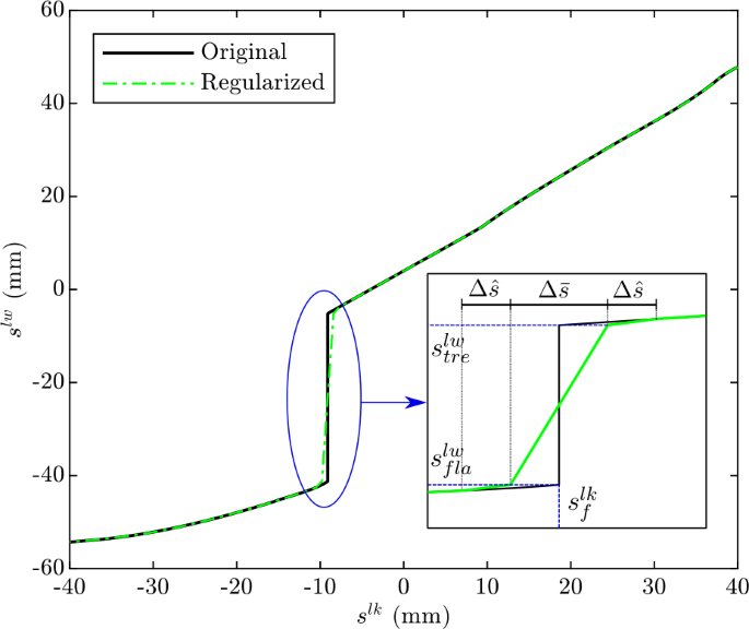

  

  Regularization of the transverse curve parameter relation for the left equivalent and real wheels when the KEC-method is used

The computation of KEC-equivalent wheel profiles requires solving Eq. (22) including no track irregularity. The authors of [16] state that the area of allowable motion for the wheel with null irregularity cannot be guaranteed to be the same as for wheels with irregularities. Later, in [24], the KEC-equivalent wheel profiles were proved to be acceptable for use in irregular tracks with accuracy.

Contact detection for two-point contact scenario

As shown in Fig. 9, with a specific value of the equivalent parameter $s_{f}^{\mathit{lk}}$, two simultaneous contact points in the real profile $s^{\mathit{lw}}_{f}$ and $s^{\mathit {lw}}_{t}$ appear, which corresponds to a two-point contact scenario (before wheel climbing). However, this discontinuity in Fig. 9 might generate an unstable numerical integration problem. Therefore, the two-point contact scenario can be simulated by adopting a smoothed transition from tread to flange with the help of a regularization approach [17]. Using the transition lengths [17] of the regularization for the tread–flange transition to account for the two-point contact scenario is critical for simulation stability and accuracy. In this work, the transition lengths used are $\Delta\hat{s} = 0.5\text{ mm}$ and $\Delta\bar{s} = 1\text{ mm}$. If the transition lengths are too small, the equation of motion matrix will be ill-conditioned, and the simulation will stall. Alternatively, if the transition lengths are larger, the simulation results may be less accurate.

Contact force computation for two-point contact scenario

One advantage of the KEC method is that contact forces on the tread and flange can be treated equally as reaction forces. The equations of motion of a railway vehicle subject to KEC constraints can also be written in the following DAE form:

$$ \begin{aligned} \mbox{$\textbf {M}$}\ddot{\mbox{$\textbf {q}$}}+\mbox{$\textbf {N}$}\boldsymbol{\lambda}&= \mbox{$\textbf {Q}$}+\mbox{$\textbf {Q}$}^{\mathit{tang}}+\mbox{$\textbf {Q}$}^{\mathit{susp}}, \\ \mbox{$\textbf {C}$}^{\mathit{KEC}}(\mbox{$\textbf {q}$},t)&=\boldsymbol{0}, \end{aligned} $$

(24)

where $\mbox{$\textbf {C}$}^{\mathit{KEC}}$ includes the KEC constraint equations for wheelset $\mbox{$\textbf {C}$}^{\mathit{wi},\mathit {KEC}}$ and forward velocity holonomic constraints, the matrix $\mbox{$\textbf {N}$}$ includes the holonomic constraint Jacobian matrix and the matrix $\mbox{$\textbf {N}$}^{\mathit{wi}}$, which represents the direction of the reaction forces and is associated with all the wheelsets in the vehicle. The wheelset KEC constraint equations $\mbox{$\textbf {C}$}^{\mathit{wi},\mathit{KEC}}$ in the dynamic simulation are the same as in Eq. (22). In this case, lateral displacement is treated as an independent coordinate, and the outputs of the nonlinear constraint equations from Eq. (22) become the vector of wheelset dependent coordinates $\mbox{$\textbf {x}$}^{\mathit{wi}} = [ z^{\mathit{wi}} \ \ \varphi ^{\mathit{wi}} \ \ s^{\mathit{lk}} \ \ s^{\mathit{rk}} ]^{T}$ [16].

The normal contact forces for the wheels are computed as the reaction forces as follows:

$$ \mbox{$\textbf {Q}$}^{\mathit{nor},\mathit{wi}} = -\mbox{$\textbf {N}$}^{\mathit {wi}}\boldsymbol{\lambda}, $$

(25)

where $\mbox{$\textbf {N}$}^{\mathit{wi}}$ represents the direction of the reaction forces and torques and is associated with the wheelset. Due to the nonlinearity, the lateral position vector $\mbox{$\textbf {s}$}^{k}$ cannot be eliminated from Eq. (22). Therefore, the reaction forces for the wheelset $\mbox{$\textbf {Q}$}^{\mathit{nor},\mathit{wi}}$ cannot be obtained using the KEC constraint Jacobian matrix $\mbox{$\textbf {Q}$}^{\mathit{nor},\mathit{wi}} \neq -\mbox{$\textbf {C}$}^{\mathit{wi},\mathit{KEC}}_{\mbox{$\textbf {q}$}}\boldsymbol{\lambda}$ in Eq. (19) [17, 24].

As shown in the left and right of Fig. 10, points $A$ and $B$ represent the wheel/tread and wheel/flange contacts when a two-point contact scenario occurs. The transition length between points $A$ and $B$ in the left of Fig. 10 corresponds to the forbidden area between points $A$ and $B$ on the left wheel profile in the right. However, in the numerical simulation, the lateral position of point $C$ in the transition length $s^{\mathit{lk}}$ of the KEC-equivalent profile (see left of Fig. 10) might be obtained by solving Eq. (22). In this case, the contact forces will be directly applied at the contact point $C$ in the forbidden area in the right of Fig. 10. Using contact force $\mbox{$\textbf {Q}$}^{\mathit{nor},\mathit{wi}}$ at point $C$ directly, the vehicle dynamic behavior might not be accurate. Therefore, the normal contact force $\mbox{$\textbf {Q}$}^{\mathit{nor},\mathit{wi}}$ is transformed into two normal contact forces at the tread-end point $\mbox{$\textbf {Q}$}_{\mathit{tre}}^{\mathit{nor},\mathit{wi}}$ and the flange starting point $\mbox{$\textbf {Q}$}_{\mathit{fla}}^{\mathit{nor},\mathit{wi}}$,

$$ \mbox{$\textbf {Q}$}^{\mathit{nor},\mathit {wi}} = \mbox{$\textbf {Q}$}_{\mathit{tre}}^{\mathit{nor},\mathit{wi}} + \mbox{$\textbf {Q}$}_{\mathit{fla}}^{\mathit{nor},\mathit{wi}}. $$

(26)

Fig. 10

(Left) Regularization of the transverse curve parameter relation for the left equivalent and real wheels; (Right) Two-point wheel/rail normal contact force computation while a regularization approach is used

2.5 Computation of tangential contact forces

In the dynamic simulation of the rail vehicle, the tangential forces and spin moment are generated between wheels and rails due to the relative motion of rolling and sliding [25]. Because it offers good computational efficiency and accuracy, the tangential contact force here was computed using Polach creep contact theory [29, 30] and treated as applied forces in the equations of motion Eqs. (16) and (24). In general, the computation of tangential contact forces requires the inputs of: (a) normal contact forces acting on the contact points, (b) relative contact velocity, (c) Kalker’s constants, and (d) coefficients of friction. In this work, the coefficient of friction was considered constant. The relative contact velocity and Kalker’s constants were computed based on the rail and wheel surface curvatures, which can be stored in a lookup table. The normal contact forces used here depends on two different situations:

• 1. If the normal contact force is computed as the reaction forces, such as the normal tread contact force with LUT method (see Eq. (19)) and normal tread or/and flange contact force with KEC method (see Eq. (25)), the normal forces obtained last time-step is used to find tangential contact force. This assumption can work is simply due to the small time-steps used in railway dynamic simulation.

• 2. If the normal contact force is computed as the applied forces, such as the normal flange contact force with LUT method (see Eq. (20)), current time-step normal contact forces are implemented for tangential contact force computation.

2.6 Computation of suspension forces

This work considers that each modeled body is accompanied by a track frame along the track centerline such that the body coordinates are defined with respect to this frame. See Fig. 11. However, when computing suspension forces, it is more convenient to employ a master track frame. Therefore, the relative kinematics for all moving bodies can be projected on the same track frame.

Fig. 11

Kinematics projected to master track frame: $\mbox{$\textbf {R}$}^{\mathit{ijt}}$ is the relative distance vector from body track frames $\mathit{it}$ to $\mathit{jt}$, $\hat{\mbox{$\textbf {u}$}}^{i}_{P}$ and $\hat{\mbox{$\textbf {u}$}}^{j}_{Q}$ are the position vectors of the points $P$ and $Q$ with respect to their body frames, $\bar{ \mbox{$\textbf {r}$}}_{P}^{i}$ and $\bar{ \mbox{$\textbf {r}$}}_{Q}^{i}$ are the position vectors of point $P$ and $Q$, which is projected into master track frame $i$

This way, the absolute position vector of a point $P$ and $Q$ in the global frame (see Fig. 11) are given by:

$$ \begin{aligned} & \mbox{$\textbf {R}$}_{P}=\mbox{$\textbf {R}$}^{\mathit{bti}}+\mbox{$\textbf {A}$}^{\mathit{bti}}( \bar{\mbox{$\textbf {r}$}}^{i}+\mbox{$\textbf {A}$}^{\mathit{bti},i}\hat{\mbox{$\textbf {u}$}}_{P}^{i}), \\ & \mbox{$\textbf {R}$}_{Q}=\mbox{$\textbf {R}$}^{\mathit{bti}}+\mbox{$\textbf {R}$}^{\mathit {ijt}}+\mbox{$\textbf {A}$}^{\mathit{btj}}( \bar{\mbox{$\textbf {r}$}}^{j}+\mbox{$\textbf {A}$}^{\mathit{btj},j}\hat{\mbox{$\textbf {u}$}}_{Q}^{j}), \end{aligned} $$

(27)

where $\mbox{$\textbf {R}$}^{\mathit{ijt}}= \mbox{$\textbf {R}$}^{\mathit{btj}}-\mbox{$\textbf {R}$}^{\mathit{bti}}$ is the relative distance vector from body track frames $\mathit{it}$ to $\mathit {jt}$, vectors $\mbox{$\textbf {R}$}^{\mathit{bti}}$ and $\mbox{$\textbf {R}$}^{\mathit{btj}}$ are the position vectors of body track frames with respect to global frame, matrices $\mbox{$\textbf {A}$}^{\mathit{bti}}$ and $\mbox{$\textbf {A}$}^{\mathit{btj}}$ are rotation matrices of body track frames, $\bar{\mbox{$\textbf {r}$}}^{i}$ and $\bar{\mbox{$\textbf {r}$}}^{j}$ are position vectors of body $i$ and $j$ with their track frames, $\hat{\mbox{$\textbf {u}$}}^{i}_{P}$ and $\hat{\mbox{$\textbf {u}$}}^{j}_{Q}$ are the position vectors of the points $P$ and $Q$ with respect to their body frames, and matrices $\mbox{$\textbf {A}$}^{\mathit{bti},i}$ and $\mbox{$\textbf {A}$}^{\mathit {btj},j}$ are the rotation matrices of body frames with respect to the body track frames. If the position vectors of points $P$ and $Q$ are referenced with respect to the master track frame with their components expressed with respect to this frame, Eq. (27) can be expressed as

$$ \begin{aligned} & \bar{ \mbox{$\textbf {r}$}}_{P}^{i}=\bar{\mbox{$\textbf {r}$}}^{i}+ \mbox{$\textbf {A}$}^{\mathit{bti},i}\hat{\mbox{$\textbf {u}$}}_{P}^{i}, \\ & \bar{ \mbox{$\textbf {r}$}}_{Q}^{i}=(\mbox{$\textbf {A}$}^{\mathit{bti}})^{T}[\mbox{$\textbf {R}$}^{\mathit{ijt}}+ \mbox{$\textbf {A}$}^{\mathit{btj}}(\bar{\mbox{$\textbf {r}$}}^{j}+\mbox{$\textbf {A}$}^{\mathit{btj},j} \hat{\mbox{$\textbf {u}$}}_{Q}^{j})]. \end{aligned} $$

(28)

Therefore, the suspension force of the spring–damper in parallel in Fig. 11 is computed as follows:

$$ \begin{aligned} & \mbox{$\textbf {Q}$}^{\mathit{susp}}_{i} = \Big(\frac {\partial d}{\partial \mbox{$\textbf {q}$}^{i}} \Big)^{T} f^{\mathit{susp}}, \\ & f^{\mathit{susp}}=\mathit{Kd}+D\dot{d}, \end{aligned} $$

(29)

where $\mbox{$\textbf {q}$}^{i}$ is the set of generalized coordinates for body $i$, $K$ is the spring stiffness, $D$ is the damping coefficient, and the deformation length of the spring $d$ is defined as:

$$ \begin{aligned} d = \sqrt{(\bar{ \mbox{$\textbf {r}$}}_{P}^{i}- \bar{ \mbox{$\textbf {r}$}}_{Q}^{i})^{T}( \bar{ \mbox{$\textbf {r}$}}_{P}^{i} - \bar{ \mbox{$\textbf {r}$}}_{Q}^{i} )} - l_{0} \end{aligned} ,$$

(30)

where $l_{0}$ is the undeformed length of the spring. The time derivative $\dot{d}$ is expressed as [31]

$$ \dot{d} = \dfrac{\partial d }{\partial \mbox{$\textbf {q}$}^{i}} \dot{\mbox{$\textbf {q}$}}^{i} .$$

(31)

The calculations of suspension forces with different suspension elements in the Manchester wagon 1 are given in Appendix A.

3 Computer simulation

The dynamic simulation of a railway vehicle integrates Eq. (16) or (24) forward in time. This procedure, developed in the framework of multibody dynamics, is described here as a function of the two wheel/rail contact methods used in this work and illustrated in Fig. 12 as follows:

• 1. Set initial conditions for the system generalized coordinates and velocities.

• 2. If using the contact LUT method, interpolate stored discrete data from the contact lookup table with two entries, $\bar{y}^{\mathit{wi}}=y^{\mathit{wi}}-\xi_{a}$ and $\xi_{g}$, and obtain the wheelset coordinates $\bar{z}^{\mathit{wi}}=z^{\mathit{wi}}+\xi_{v}$, $\bar{\varphi}^{\mathit{wi}}={\varphi}^{\mathit{wi}}+\xi_{c}/2L_{r}$, and surface parameters $s^{\mathit{lw}}$, $s^{\mathit{lr}}$, $s^{\mathit{rw}}$, $s^{\mathit{rr}}$. Normal contact forces in the tread are computed as reaction forces associated with contact constraints, while in this work, the normal contact forces for the flange are computed as a Hertzian penetration-based model.

• 3. If using the KEC method, solve the KEC constraint equations from Eq. (22) to get the wheelset coordinates $z^{\mathit{wi}}$, $\varphi^{\mathit{wi}}$, and KEC-profile positions $s^{\mathit{lk}}$, $s^{\mathit{rk}}$ with inputs $y^{\mathit{wi}}$ and track irregularities $y^{\mathit{lir}}$, $y^{\mathit{rir}}$, $z^{\mathit{lir}}$, $z^{\mathit{rir}}$. Interpolate stored discrete data from the KEC-lookup table to get surface parameters $s^{\mathit{lw}}$ and $s^{\mathit{lr}}$ with the entry of $s^{\mathit{lk}}$ and $s^{\mathit{rw}}$ and $s^{\mathit{rr}}$ with the entry of $s^{\mathit{rk}}$. Normal contact forces on the tread and the flange are treated equally as the reaction forces. The two-point contact scenario can be simulated with a smooth transition of the normal contact forces from tread to flange.

• 4. Include the contact force vectors at each wheel, suspension force vectors (primary and secondary), Newton–Euler generalized forces and quadratic-velocity generalized inertia forces into the vector of external forces of the system. Solve the equations of motion of the railway vehicle to get the generalized accelerations $\ddot{\mbox{$\textbf {q}$}}$.

• 5. Return the new generalized positions $\mbox{$\textbf {q}$}$ and velocities $\dot{\mbox{$\textbf {q}$}}$ at time $t+\Delta t$ with the numerical integration subroutine.

• 6. Go to step 2 or 3 until the analysis is finished.

Fig. 12

Flow chart of simulation procedure

4 Integration methods

The numerical integration method can be divided into explicit and implicit integration. The decision to use an explicit or implicit method depends on the studied system. In the explicit method, the calculation of the variables at each time step requires the solution of the linear equations that are functions of the values of the variables in previous time steps. In the implicit method, the calculation of the variables at each time step requires the solution of the nonlinear equations that are functions of the values of the variables in the current and the previous time steps. Therefore, the implicit method uses iteration to solve nonlinear equations at each time step.

This study uses a fourth order Runge–Kutta method as the fixed-step-size explicit integrator [32]. It is a single step method, and four function evaluations are required in each integration step. As an alternative time-integration scheme, the predictor–corrector ABM method is used as the fixed-step-size in this work. It allows determining the errors in each iteration step (local truncation error) and a correction term can be included. The Adams–Bashforth–Moulton scheme can be written as follows:

$$ \begin{aligned} \mbox{$\text{(Predictor)}$}\ \mbox{$\textbf {y}$}_{n+1}&=\mbox{$\textbf {y}$}_{n}+ \Delta t(55\mbox{$\textbf {f}$}(t_{n},\mbox{$\textbf {y}$}_{n})-59\mbox{$\textbf {f}$}(t_{n-1}, \mbox{$\textbf {y}$}_{n-1})+37\mbox{$\textbf {f}$}(t_{n-2},\mbox{$\textbf {y}$}_{n-2}) \\ &-9\mbox{$\textbf {f}$}(t_{n-3}, \mbox{$\textbf {y}$}_{n-3}))/24, \\ \mbox{$\text{(Corrector)}$}\ \mbox{$\textbf {y}$}_{n+1}&=\mbox{$\textbf {y}$}_{n}+\Delta t(9 \mbox{$\textbf {f}$}(t_{n+1},\mbox{$\textbf {y}$}_{n+1}+19\mbox{$\textbf {f}$}(t_{n},\mbox{$\textbf {y}$}_{n})-5 \mbox{$\textbf {f}$}(t_{n-1},\mbox{$\textbf {y}$}_{n-1}))/24, \end{aligned} $$

(32)

where ${t}_{n-0..3}$ and $\mbox{$\textbf {y}$}_{n-0...3}$ are the three previous time steps and state variables.

The ABM is a multistep method that has two function evaluations in each integration step, the predictor and the corrector. Compared to the RK4 with four function evaluations, the ABM should be twice as fast.

The Matlab built-in function $ode45$ is typically selected as the variable-step-size explicit integrator, as it can provide an acceptable solution in most cases. It is a single-step explicit integrator based on the Runge–Kutta (4,5) formula (Dormand–Prince method). For stiff systems, the solution time with $ode45$ increases, and other Matlab built-in time integrators schemes such as $ode15s$ can perform better; $ode15s$ is a variable order and variable-step-size implicit solver based on numerical differentiation formulas (NDFs) of orders 1 to 5. Optionally, the maximum order (5) can be reduced or a backward difference formulation can be used [33].

The railway vehicle models usually contain stiff springs for suspension components or contact forces modeling. The explicit integration methods, such as RK4, are not suitable for a stiff problem. In many cases, the explicit integration method is conditionally stable and it need least effort for one time integration step. However, the method requires a small time-step size to solve the stiff problem and makes the simulation less efficient [34]. Furthermore, the predictor–corrector ABM method includes the previous step information to prevent the numerical instability. The Matlab ode45 is based on Runge–Kutta algorithm and has similar features as the RK4 for a stiff problem. The Matlab ode15s is based on NDF formulation, where the time-step and solution order can be changed. These features are desired in the stiff problem solution, as dynamically adjusting these parameters allows obtaining the solution efficiently. However, it requires the iterative solution for the nonlinear equations and the update of the Jacobian matrix at each time step. As the number of unknowns gets larger, the numerical effort for the update of Jacobian matrices starts to be more expensive [23].

5 Simulation results

5.1 Vehicle model description

This section describes the vehicle model used in the numerical simulations of Sect. 3, which is based on the Manchester wagon used in Iwnick [3] as a benchmark. Figure 13 illustrates the various components of the vehicle formed by one carbody, two bogie frames and four wheelsets with primary and secondary suspension elements.

Fig. 13

Three-dimensional Manchester wagon: (a) side view; (b) front view

The mass and inertia properties of the different bodies are presented in Table 2. The wheel and rail profiles used for the contact lookup table and computation of the KEC profiles are the S1002 wheel and LB140-Area rail profiles shown in Fig. 14, which present a unique two-point contact scenario in the tread–flange transition. Wheel and rail profile positioning with respect to the track centerline ($L_{w}$, $L_{r}$), rail inclination ($\beta$) and wheel nominal radius ($r_{0}$) are given in Table 1. The coefficient of friction for the wheel rail tangential contact force is $\mu=0.2364$ and the Hertzian stiffness and damping constant for flange contact with the LUT method are listed in Table 3.

Fig. 14

Real wheel/rail profile combination that shows two-point contact scenario and LB-140-area rail profile with S1002 wheel profile

Table 2 Simulation parameters for the vehicle

Table 3 Hertzian stiffness and damping constant for flange contact with LUT method

The primary and secondary suspension shown in Fig. 13 involves a total of 48 elements classified into springs and dampers in series, spring and dampers in parallel, and bumpstops, with their stiffness and damping properties given in Table 4.

Table 4 Main parameters of suspension elements in the simulation

Track irregularities are generated using analytical expressions of the power spectral density functions (PSD) [35]. The alignment, vertical profile, gauge variation, and cross level are shown in Fig. 15.

Fig. 15

Track irregularities

5.2 Validation

In this section, the 3D multibody model of the railway vehicle is implemented in commercial simulation software, Universal Mechanism (UM) [36] to validate that implemented in Matlab software. For both the KEC and LUT methods in Matlab software and UM commercial simulation software, the fixed-step-size integrator ABM with time step size $\Delta t=1\text{ ms}$ is used for all approaches. In addition, the Hertzian contact stiffness at the flange for the LUT method is $K^{\mathit{hertz}}=1\cdot10^{10}$ $\text{N}/\text{m}^{1.5}$. A numerical comparison of three different case studies is presented: (1) single wheelset on a curved track without track irregularities, (2) the Manchester vehicle on a curved track without track irregularities, and (3) the Manchester vehicle on a curved track with track irregularities.

Single wheelset on a curved track without track irregularities

In the first case, the single wheelset is simulated at a constant forward velocity of $V=10\text{ m}/\text{s}$ (36 km/h) on a 120 m track without irregularities constructed of the following three segments: a 30 m tangent, a 50 m transition, and a 40 m left curve segment with different values of curve radius as shown in Fig. 16.

Fig. 16

Track geometries with 120 m traveled distance. Lines perpendicular to the track geometry show the transition points of the track segments

Figure 17 shows the comparison of the lateral displacement and yaw angle of the wheelset with the KEC and LUT methods and UM. The achievement of the steady curving can be observed when the vehicle enters into transition curve (see grey area). In addition, with different values of curve radius, the traveled distance where steady curving starts is different. The steady curving results are quantified in Table 5. The results of lateral displacement and yaw angle show good agreement between both of the examined methods and UM, except for the yaw angle, which is about 2 mrad bigger when using UM on the radius $R=300\text{ m}$ curve track. That is mainly because the planar contact approach is implemented into the KEC and LUT methods, but in UM, the 3D elastic contact approach is utilized for the tread and flange contacts.

Fig. 17

Comparison of the lateral displacement and yaw angle of the single wheelset vehicle as it negotiates different radius tracks with constant forward velocity $V=10\text{ m}/\text{s}$. The white area represents the tangent segment, the grey area represents the transition curve segment, and the blue area represents the left curve segment

Table 5 Vehicle coordinates during steady curving, when a single wheelset vehicle negotiates different radius tracks with constant forward velocity $V=10\text{ m}/\text{s}$

Manchester wagon on a curved track without track irregularities

In the second case, the Manchester wagon is simulated at a constant forward velocity of $V=20\text{ m}/\text{s}$ (72 km/h), on a 500 m track without irregularities formed by the following three segments: a 100 m tangent, a 50 m transition, and a 350 m left curve of $R=500\text{ m}$ radius segment (see Fig. 18).

Fig. 18

Track geometries on the 500 m traveled distance with an $R=500\text{ m}$ radius curved track

Figures 19 and 20 show a comparison of lateral displacements and yaw angles for the vehicle wheelsets, bogies, and car body, when using the KEC and LUT methods and UM. Table 6 lists the quantities of the steady curving results. Again, the results of lateral displacement and yaw angle show good agreement. A steady curving motion is achieved when the vehicle enters into the transition curve. According to the lateral displacement of the four wheelsets, the front wheelsets of both bogies can experience flange contact when negotiating the curve (blue area in the figure), and the rear wheelsets do not.

Fig. 19

Comparison of kinematics of four wheelsets when the vehicle negotiates the $R=500\text{ m}$ radius track without track irregularities with constant forward velocity $V=20\text{ m}/\text{s}$

Fig. 20

Comparison of kinematics of bogies and car body – the information is the same as that shown by Fig. 19

Table 6 Vehicle coordinates during steady curving when a Manchester wagon negotiates an $R=500\text{ m}$ radius curved track without irregularities with constant forward velocity $V=20\text{ m}/\text{s}$

Manchester wagon on a curved track with track irregularities

In the last case, the Manchester wagon is simulated at a constant forward velocity of $V=20\text{ m}/\text{s}$ (72 km/h) on a 500 m track (see Fig. 18) with irregularities. Figures 21 and 22 show a comparison of the lateral displacement and yaw angle for the vehicle wheelsets, bogies, and car body when using the KEC and LUT methods and UM. The results of lateral displacement and yaw angle are almost identical with the results on the irregular track. According to the lateral displacement of the two wheelsets, steady curving motion is not achieved because of the track irregularities.

Fig. 21

Comparison of kinematics of four wheelsets when the vehicle negotiates the $R=500\text{ m}$ radius track with track irregularities and constant forward velocity $V=20\text{ m}/\text{s}$

Fig. 22

Comparison of kinematics of bogies and car body, the information is same as in Fig. 21

5.3 Computational efficiency

In this case, the Manchester wagon is simulated at a constant forward velocity of $V=20\text{ m}/\text{s}$ (72 km/h), on the same 500 m track as shown in Fig. 18 with irregularities. The computational efficiency of the LUT method is compared to that of the KEC method using different integration methods. The comparison was carried out on an Intel Core i5 laptop with a 2.5 GHz CPU and Matlab 2018b. The Mex functions written in C or Fortran were not used to improve computational efficiency in Matlab. To determine the computational time, each case is simulated five times, and the calculated simulation time was as the average value of the five runs. The computation times for the five runs for each case are listed in Appendix B. Two fixed-step-size integrators, explicit RK4 and predictor–corrector ABM, and two variable-step-size Matlab built-in function integrators, explicit $ode45$ and implicit $ode15s$, were applied to compare computational efficiency.

According to the Hertz contact theory [25], the flange Hertzian stiffness for the wheel–rail profile combination shown in Fig. 14 is $K^{\mathit{hertz}}=7.075\cdot10^{13}~\text{N}/\text{m}^{1.5}$ with the Poisson’s ratio $\nu=0.28$ and Young’s modulus $E=2.1\cdot10^{11}$ $\text{N}/\text{m}^{2}$. Since the location of the flange contact points remains the same when the two-point contact scenario occurs, the constant flange contact stiffness parameters are considered for the hybrid method in the contact lookup table. Computational costs and function evaluations of the vehicle simulation with flange Hertzian stiffness $K^{\mathit{hertz}}=7.075\cdot 10^{13}~\text{N}/\text{m}^{1.5}$ for the LUT method are listed in Table 7. With step size $\Delta t=1\text{ ms}$, RK4 and ABM failed to converge at same time as when flange occurs. In addition, the variable-step-size explicit integrator $ode45$ only succeeds when the absolute and relative tolerance is smaller than $1\cdot 10^{-8}$ and the variable-step-size implicit integrator $ode15s$ only succeeds when the absolute and relative tolerance is smaller than $1\cdot 10^{-7}$. This is because having the high-magnitude Hertzian parameter, $K^{\mathit {hertz}}=7.075\cdot10^{13}~\text{N}/\text{m}^{1.5}$, results in a stiff system of ordinary differential equations, and some variations of the equation significantly impact the solution. If the time step and/or tolerances are too large, the first impact between the wheel flange and rail head may result in a substantial penetration depth, which leads to a numerically instability and failure of the time integration. Therefore, a large number of time steps are needed to solve the problem, which results in high computational cost.

Table 7 Computation cost for track radius $R=500\text{ m}$ with forward velocity $V=20\text{ m}/\text{s}$ on a 500 m track using LUT method with different integrators – the Hertzian stiffness at the flange for LUT method is $7.075\cdot10^{13}$ $\text{N}/\text{m}^{1.5}$

Under the assumption that the contacting bodies behave like infinite semispaces, the Hertzian stiffness of $K^{\mathit{hertz}}=7.075\cdot10^{13}~\text{N}/\text{m}^{1.5}$ might be higher than the real value. In fact, reducing the value of Hertzian stiffness is realistic because the influence of flange flexibility is not considered. In what follows, different values of flange contact stiffness will be presented. Computational cost and function evaluations of the vehicle simulation with different values of flange Hertzian stiffness for LUT method are compared against KEC method in Fig. 23. The computation time of five runs for each case are listed in Tables 12, 13, 14, 15, 16. When using variable-step-size integrators, ode15s and ode45, the KEC method is much superior to the LUT method with higher flange contact stiffness (such as $K^{\mathit{hertz}}=1\cdot10^{11}~\text{N}/\text{m}^{1.5}$ and $1\cdot10^{12}~\text{N}/\text{m}^{1.5}$). This is due to the large value of stiffness that leads to a stiff system of ordinary differential equations and increases the computational effort during the simulation. It is true that stiff integrators (ode15s) are more expensive. But in case of stiff systems, they lead to a stable solution that is not sometimes possible or take even more time in the case of nonstiff integrators (ABM and RK4). When working with lower flange stiffness $K^{\mathit{hertz}}=1\cdot10^{10}~\text{N}/\text{m}^{1.5}$ and $1\cdot10^{9}~\text{N}/\text{m}^{1.5}$, the LUT method shows better performance in computational efficiency.

Fig. 23

Computation cost for track radius $R=500\text{ m}$ with forward velocity $V=20\text{ m}/\text{s}$ on a 500 m track by using both methods with different integrators

5.4 Accuracy

Table 8 lists a comparison of maximum and average errors of lateral displacement between LUT and KEC methods when using different integrators, with the Manchester wagon simulated at a constant forward velocity of $V=20\text{ m}/\text{s}$ (72 km/h) on a 500 m track with irregularities. See Fig. 18. Different values of flange stiffness are considered at the wheel flange. The fixed step sizes are $\Delta t=1\text{ ms}$ for fixed-step-size integrators RK4 and ABM. The maximum step size is $\Delta t=1\text{ ms}$ for Matlab integrators $ode45$ and $ode15s$. The absolute and relative tolerance for $ode45$ and $ode15s$ is $1\cdot10^{-6}$. The error between both methods is computed as

$$ \mathit{Error} = \dfrac{|y^{\mathit{wh}}_{\mathit{KEC}}-y^{\mathit{wh}}_{\mathit {LUT}}|}{\max (|y^{\mathit{wh}}_{\mathit{LUT}}|)} , $$

(33)

where $y^{\mathit{wh}}_{\mathit{KEC}}$ is the lateral displacement for the KEC method within a 25 s simulation, and $y^{\mathit{wh}}_{\mathit{LUT}}$ is for the LUT method. Some conclusions can be made based on the numerical results from Table 8:

• For all integrators, the lower flange stiffness for the LUT method (especially $K^{\mathit{hertz}}=1\cdot10^{9}$ N/m^1.5) results in higher maximum and average absolute errors. This is due to the low flange stiffness that results in large flange to rail head indentations.

• Compared to the other integrators, the ABM errors are much higher when selecting a large value of the flange contact stiffness $K^{\mathit{hertz}}=1\cdot10^{12}$ N/m^1.5. This is because constant time-step integrators are not appropriate for impact problems. As shown in Fig. 24, the flange indentation and normal contact forces become artificially large for the ABM integrator.

  Fig. 24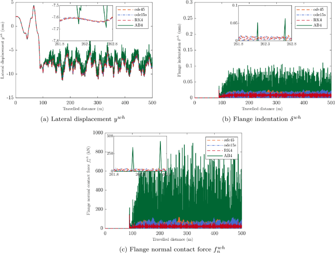

  

  Comparison of lateral displacement, flange indentation, and normal contact force with the LUT method when using ABM, RK4, $ode45$ and $ode15s$. The fixed step sizes are $\Delta t=1\text{ ms}$ for fixed-step-size integrators RK4 and ABM. The maximum step size is $\Delta t=1\text{ ms}$ for the Matlab integrators $ode45$ and $ode15s$. The absolute and relative tolerance for $ode45$ and $ode15s$ is $1\cdot10^{-6}$. Flange contact stiffness $K^{\mathit{hertz}}=1\cdot10^{12}$ $\text{N}/\text{m}^{1.5}$

Table 8 Maximum and average errors of lateral displacement between the LUT and KEC methods

As shown in Fig. 25, the use of a low stiffness ($K^{\mathit{hertz}}=1\cdot10^{9}$ N/m^1.5) helps to simulate the vehicle motion. However, low stiffness results in high indentations (around 0.75 mm) that can be considered as physically inadmissible. Even though the flange indentations are different for different flange contact stiffnesses $K^{\mathit{hertz}}$ in Fig. 25, the resulting flange normal contact forces $F_{\mathit{hertz}}$ are on average almost the same. However, the higher the stiffness, the higher the force oscillations.

Fig. 25

Comparison of flange indentation and normal contact force with LUT method when using ABM with step size $\Delta t =0.1\text{ ms}$. Different flange contact stiffnesses are considered

5.5 The effect of the refinement for the KEC and LUT tables on the computational efficiency

The use of lookup table for both LUT and KEC approaches requires generating a precalculated table which tabulates the values of the different parameters and variables into a set of nodal points. Later in the dynamic simulations, the required parameters or variables for the dynamic analysis are obtained by using linear interpolation between the stored data. The KEC table has only one entry, the lateral wheel parameter $s^{\mathit{lk}}$ or $s^{\mathit{rk}}$. In addition, the LUT table has two entries, gauge variation irregularity $\xi_{g}$ and wheelset lateral displacement $y^{w}$. In this section, each KEC table is refined by increasing the number of points from $465\times1$ to $5001\times1$ as listed in Table 9. Furthermore, each LUT table is refined by increasing the number of points from $361\times11$ to $721\times11$ as listed in Table 10.

Table 9 Notes of lookup table information for KEC tables before and after refinement

Table 10 Notes of lookup table information for both LUT and KEC tables

The refinement of lookup tables tends to increase the precalculation time and the computer storage while it is assumed to improve the accuracy of the interpolated values [15]. To verify if the refinement of lookup tables can improve the computational efficiency, Fig. 26 compares the computation cost by using KEC and LUT methods with the flange Hertzian stiffness $1\cdot10^{10}$ $\text{N}/\text{m}^{1.5}$. The computation time of five runs for each refinement case are listed in Tables 17–18. The results indicate that the refinement of both KEC and LUT tables can slightly improve the computational efficiency in most particular cases (14 out of 18).

Fig. 26

Computation cost for track radius $R=500\text{ m}$ with forward velocity $V=20\text{ m}/\text{s}$ on 500 m track by using both KEC and LUT methods with and without refinement

Table 11 lists the computational costs and function evaluations of the vehicle simulation with flange Hertzian stiffness $K^{\mathit{hertz}}=7.075\cdot10^{13}~\text{N}/\text{m}^{1.5}$ for the LUT method after refinement. Compared to the result before refinement from Table 7, it can be concluded that the refinement only helps $ode15s$ and $ode45$ to smooth the numerical integration that increases the maximum tolerance to 10 times bigger.

Table 11 Computation cost for track radius $R=500\text{ m}$ with forward velocity $V=20\text{ m}/\text{s}$ on 500 m track by using the LUT method after refinement, the Hertzian stiffness at flange is $7.075\cdot10^{13}$ $\text{N}/ \text{m}^{1.5}$

6 Conclusion

Two constraint-based formulations for the wheel/rail contact simulation were studied in terms of their accuracy and computational efficiency based on the Manchester wagon 1 model. Two fixed-step-size integrators, RK4 and predictor–corrector-based ABM, and two variable-step-size Matlab integrators, $ode15s$ and $ode45$, were used to carry out the comparison.

The studied contact models are the KEC and LUT methods. The differences between each approach can be summarized as follows:

• 1. Contact detection for the LUT method is based on an offline approach where the contact points are determined by interpolating a predefined lookup table. The KEC method is an online contact detection approach where the exact position of the contact points can be determined from the online solution of the KEC constraints.

• 2. The second difference is the computation of normal contact forces at the flange. For the LUT method, the normal contact forces are defined in terms of stiffness and damping ratio using Hertz’s contact theory. This implies that computational efficiency and numerical stability will be affected by the large magnitude values of the stiffness parameters. However, with using the KEC method, the normal contact forces are determined through Lagrange multipliers that avoid the numerical disadvantages in the case of stability using high values of contact stiffnesses.

Numerical simulations of vehicle dynamics have been carried out in different case studies with and without track irregularities. Comparison between the kinematic results obtained by Matlab and the commercial simulation software UM has allowed a reliable validation of both the LUT and KEC methods. The performance of both approaches is compared in terms of efficiency and accuracy. The KEC method is faster (more computationally efficient) than the LUT method when using all the studied integrators (up to $20\%$). Also, as expected for the LUT method, results are more accurate when Hertzian stiffness is lower. The integrators $ode15s$ and $ode45$ showed better efficiency compared to the integrators RK4 and ABM, only when flange contact stiffness $K^{\mathit{hertz}}$ is lower than $1\cdot10^{10}$ $\text{N}/\text{m}^{1.5}$. As for the KEC method, the integrators $ode15s$ and $ode45$ are faster than the fixed-step-size case under some specific tolerances.

Appendices

Appendix A: Elements used for the suspension systems

The bumpstop forces $f$ can be parameterized as a continuous functions (cubic splines in this work) of the relative displacement $d$, as shown in Fig. 27.

Fig. 27

The nonlinear stiffness for longitudinal bumpstop

Appendix B: Computational time for five runs

Table 12 Computation cost for track radius $R=500\text{ m}$ with forward velocity $V=20\text{ m}/\text{s}$ on 500 m track by using the LUT method with Hertzian stiffness at flange $1\cdot10^{9}$ $\text{N}/\text{m}^{1.5}$

Table 13 Computation cost for track radius $R=500\text{ m}$ with forward velocity $V=20\text{ m}/\text{s}$ on 500 m track by using the LUT method with Hertzian stiffness at flange $1\cdot 10^{10}$ $\text{N}/\text{m}^{1.5}$

Table 14 Computation cost for track radius $R=500\text{ m}$ with forward velocity $V=20\text{ m}/\text{s}$ on 500 m track by using the LUT method with Hertzian stiffness at flange $1\cdot 10^{11}$ $\text{N}/\text{m}^{1.5}$

Table 15 Computation cost for track radius $R=500\text{ m}$ with forward velocity $V=20\text{ m}/\text{s}$ on 500 m track by using the LUT method with Hertzian stiffness at flange $1\cdot10^{12}$ $\text{N}/\text{m}^{1.5}$

Table 16 Computation cost for track radius $R=500\text{ m}$ with forward velocity $V=20\text{ m}/\text{s}$ on 500 m track by using the KEC method with different integrators

Table 17 Computation cost for track radius $R=500\text{ m}$ with forward velocity $V=20\text{ m}/\text{s}$ on 500 m track by using the KEC method with different integrators after refinement

Table 18 Computation cost for track radius $R=500\text{ m}$ with forward velocity $V=20\text{ m}/\text{s}$ on 500 m track by using the LUT method with Hertzian stiffness at flange $1\cdot10^{10}$ $\text{N}/\text{m}^{1.5}$ after refinement

References

Bruni, S., Meijaard, J.P., Rill, G., Schwab, A.L.: State-of-the-art and challenges of railway and road vehicle dynamics with multibody dynamics approaches. Multibody Syst. Dyn. 29(1), 1–32 (2020)
Ferreira, J., Flores, P., Marques, F.: On the utilization of simplified methodologies for the wheel–rail contact. In: International Symposium on Multibody Systems and Mechatronics. Springer, Cham (2021)
Iwnick, S.: Manchester benchmarks for rail vehicle simulation. Veh. Syst. Dyn. 30(3–4), 295–313 (1998)
Bezin, Y., Pålsson, B.A.: Multibody simulation benchmark for dynamic vehicle–track interaction in switches and crossings: modelling description and simulation tasks. Veh. Syst. Dyn. 1–16 (2021). https://doi.org/10.1080/00423114.2021.1942079
Shabana, A.A., Zaazaa, K.E., Escalona, J.L., Sany, J.R.: Development of elastic force model for wheel/rail contact problems. J. Sound Vib. 269(1–2), 295–325 (2004)
Magalhães, H., Marques, F., Liu, B., Antunes, P., Pombo, J., Flores, P., Ambrósio, J., Piotrowski, J., Bruni, S.: Implementation of a non-Hertzian contact model for railway dynamic application. Multibody Syst. Dyn. 48(1), 41–78 (2020)
Marques, F., Magalhães, H., Pombo, J., Ambrósio, J., Flores, P.: A three-dimensional approach for contact detection between realistic wheel and rail surfaces for improved railway dynamic analysis. Mech. Mach. Theory 149, 103825 (2020)
Liu, B., Bruni, S.: Comparison of wheel–rail contact models in the context of multibody system simulation: Hertzian versus non-Hertzian. Veh. Syst. Dyn. 1–21 (2020). https://doi.org/10.1080/00423114.2020.1847297
Sugiyama, H., Suda, Y.: On the contact search algorithms for wheel/rail contact problems. J. Comput. Nonlinear Dyn. 4(4), 041001 (2009)
Sugiyama, H., Araki, K., Suda, Y.: On-line and off-line wheel/rail contact algorithm in the analysis of multibody railroad vehicle systems. J. Mech. Sci. Technol. 23(4), 991–996 (2009)
Sugiyama, H., Sekiguchi, T., Matsumura, R., Yamashita, S., Suda, Y.: Wheel/rail contact dynamics in turnout negotiations with combined nodal and non-conformal contact approach. Multibody Syst. Dyn. 27, 55–74 (2012)
Escalona, J.L., Aceituno, J.F.: Multibody simulation of railway vehicles with contact lookup tables. Int. J. Mech. Sci. 155, 571–582 (2019)
Piotrowski, J., Liu, B., Bruni, S.: The Kalker book of tables for non-Hertzian contact of wheel and rail. Veh. Syst. Dyn. 55(6), 875–901 (2017)
Piotrowski, J., Bruni, S., Liu, B., Gialleonardo, E.D.: A fast method for determination of creep forces in non-Hertzian contact of wheel and rail base on a book of tables. Multibody Syst. Dyn. 45, 169–184 (2019)
Marques, F., Magalhães, H., Liu, B., Pombo, J., Flores, P., Ambrósio, J., Piotrowski, J., Bruni, S.: On the generation of enhanced lookup tables for wheel–rail contact models. Wear 434–435, 202993 (2019)
Escalona, J.L., Aceituno, J.F., Urda, P., Balling, O.: Railway multibody simulation with the knife-edge-equivalent wheel–rail constraint equations. Multibody Syst. Dyn. 48(4), 373–402 (2020)
Aceituno, J.F., Urda, P., Briales, E., Escalona, J.L.: Analysis of the two-point wheel–rail contact scenario using the knife-edge-equivalent contact constraint method. Mech. Mach. Theory 148, 103803 (2020)
Muñoz, S., Aceituno, J.F., Urda, P., Escalona, J.L.: Multibody model of railway vehicles with weakly coupled vertical and lateral dynamics. Mech. Syst. Signal Process. 115, 570–592 (2019)
Schupp, G., Weidemann, C., Mauer, L.: Modelling the contact between wheel and rail within multibody system simulation. Veh. Syst. Dyn. 41(5), 349–364 (2004)
Meli, E., Magheri, S., Malvezzi, M.: Development and implementation of a differential elastic wheel–rail contact model for multibody applications. Veh. Syst. Dyn. 49(6), 969–1001 (2011)
Zhai, W.: Two simple fast integration methods for large-scale dynamic problems in engineering. Int. J. Numer. Methods Eng. 39(24), 4199–4214 (1996)
Baeza, L., Roda, A., Nielsen, J.C.: Railway vehicle/track interaction analysis using a modal substructuring approach. J. Sound Vib. 293(1–2), 112–124 (2016)
Arnold, M., Fuchs, A., Führer, C.: Efficient corrector iteration for DAE time integration in multibody dynamics. Comput. Methods Appl. Mech. Eng. 195(50–51), 6958–6973 (2006)
Escalona, J.L., Yu, X., Aceituno, J.F.: Wheel–rail contact simulation with lookup tables and KEC profiles: a comparative study. Multibody Syst. Dyn. 52(4), 339–375 (2021). https://doi.org/10.1007/s11044-020-09773-7
Shabana, A.A., Zaazaa, K.E., Sugiyama, H.: Railroad Vehicle Dynamics: A Computational Approach. CRC Press, Boca Raton (2007)
Popp, K., Schiehlen, W.: Ground Vehicle Dynamics. Springer, Berlin (2010)
Goldsmith, W.: Impact: The Theory and Physical Behaviour of Colliding Solids. Edward Arnold Ltd., London, England (1960)
Flores, P., Ambrósio, J.: On the contact detection for contact–impact analysis in multibody systems. Multibody Syst. Dyn. 24(1), 103–122 (2010)
Polach, O.: A fast wheel–rail forces calculation computer code, Veh. Syst. Dyn. 33 (Proceedings of the 16th IAVSD Symposium held in Pretoria, South Africa, August 30 – September 3, 1999) 728–739 (1999). https://doi.org/10.1080/00423114.1999.12063125
Polach, O.: Creep forces in simulations of traction vehicles running on adhesion limit. Wear 258(7–8), 992–1000 (2005) https://doi.org/10.1016/j.wear.2004.03.046
Shabana, A.A.: Computational Dynamics. John Wiley & Sons, Inc, United Kingdom (2009)
Ashino, R., Nagase, M., Vaillancourt, R.: Behind and beyond the Matlab ODE suite. Comput. Math. Appl. 40(4–5), 491–512 (2000)
Shampine, L.F., Reichelt, M.W.: The Matlab ODE suite. SIAM J. Sci. Comput. 18(1), 1–12 (1997)
Burgermeister, B., Arnold, M., Esterl, B.: DAE time integration for real-time applications in multi-body dynamics. ZAMM–J. Appl. Math. Mech./Z. Angew. Math. Mech.: Appl. Math. Mech. 86(10), 759–771 (2006)
Claus, H., Schiehlen, W.: Modeling and simulation of railway bogie structural vibrations. Veh. Syst. Dyn. 29, 538–552 (1998)
Pogorelov, D.Y.: Simulation of rail vehicle dynamics with universal mechanism software. In: Rail Vehicle Dynamics and Associated Problems, pp. 13–58. Silesian University of Technology, Gliwice (2005)
Acknowledgements
The authors thank for the support given by Business of Finland under the SmartTram-LUT project with reference 6292/31/2018. In addition, the authors thank for the help of the Andalusian Regional Government, in Spain, under the PAIDI 2020 program with project reference P18-RT-1772. All this support is gratefully acknowledged.
Funding
Open Access funding provided by LUT University (previously Lappeenranta University of Technology (LUT)).
Author information
Authors and Affiliations
Corresponding author
Ethics declarations
Conflicts of interest
The authors declare that there is no conflict of interest to this work.
Additional information
Publisher’s Note
Springer Nature remains neutral with regard to jurisdictional claims in published maps and institutional affiliations.