The large key space image encryption algorithm based on modulus synchronization between real and complex fractional-order dynamical systems

Abstract

This paper constructs and analyzes the dynamical properties of a new fractional-order real hyper-chaotic system and its corresponding complex variable system. A thorough analysis was done by employing stability of equilibrium points, phase plots, Lyapunov spectrum, and bifurcation analysis for the consequences of varying fractional-order derivative and parameter values on the system. For the first time, a modulus synchronization scheme is proposed to synchronize real and complex fractional-order dynamical systems. Based on Lyapunov stability theory, non-linear controllers are designed to achieve the proposed modulus synchronization scheme. A new modulus synchronization encryption algorithm with a large key space size for digital images is introduced for the application. The experimental results and analysis validate the desired algorithm. Also, we compare our result of the new encryption algorithm with the previously published literature and verify the efficacy of the considered scheme. Numerical simulations are given to validate the theoretical analysis

1 Introduction

In the digital world, digital or multimedia data security becomes more critical since they are easily transmitted over the network via insecure channels to help recent communication and social networking technologies. A well-secured encryption scheme is essential for multimedia data communication to protect and stop the misuse of multimedia data. In information communication, the digital image is an essential carrier of information. The encryption algorithms using chaotic systems are more effective and secure than traditional encryption algorithms due to some important features of chaotic systems like sensitivity to initial conditions, simple analytic description, ergodicity, and high complex behavior, which are more favorable to data security. Image encryption algorithms based on chaotic systems have been investigated [16, 17, 25, 26, 34, 40,41,42,43] with an experimental analysis and their outcomes have been reported. The key space size plays a more vital role in all encryption algorithms since the security level depends on key space size. If the size of the key space is very large, then the hackers should not be able to hack the keys easily. The existing image encryption algorithms [16, 17, 25, 26, 34, 40,41,42,43] have key space size is nearly equal to 2⁶⁰⁰. So, it is essential to propose an encryption algorithm with a large key space size.

A strategy for underwater image enhancement has been proposed in [10] by using the methodology of Contrast-Limited Adaptive Histogram Equalization (CLAHE) and Percentile to improve the quality of the image outcome. The object recognition results and their applications using several deep learning methods have been described in [4]. Further, analysis results of various techniques for object recognition have been reported. The major survey of deep learning and its significant application domains in the various field has been presented in [9]. A new scheme for printer attribution [22] has been constructed with the support of utilizing Speeded Up Robust Features and Oriented Fast Rotated and BRIEF feature descriptors. At very first, source camera and source mobile detection evaluation were attempted in [13]. The passive approach has been established to fix the document source printer in [12] and adaptive boosting-bootstrap aggregating methodologies have been proposed to improve the level of classification accuracy.

Fractional calculus [6, 35] can be employed as an important mathematical instrument for modeling of practical systems. The dynamical behaviors of many practical systems have been described by fractional differential equations, such as viscoelastic system [2], kinetic equations [36] and dynamo theory [32]. In recent decades, the study of chaos, control, and synchronization [19, 21] in fractional-order systems has been gaining interest due to their applications in cryptography. In particular, fractional-order dynamical systems have been applied to develop an algorithm for encryption-decryption of multimedia data; for instance, fractional-order hyper-chaotic systems have been utilized for color image encryption algorithm [15, 17, 20, 34], synchronized fractional-order King Cobra chaotic systems have been applied for image encryption technique [31], fuzzy fractional integral sliding mode control based image encryption algorithm has been presented in [3], robust synchronization of mismatched fractional-order dynamical systems have been applied to an audio encryption algorithm in [33], and a video encryption algorithm based on a fractional-order hyperchaotic system has been proposed in [14].

Apart from real variable fractional-order systems, the complex variable fractional-order systems received very much attention because of their existence in rotating fluids, electronic circuits, detuned lasers and many more. In this direction, chaos has been identified in fractional-order complex Lorenz system [29] and fractional-order complex Chen system [28]. The cluster synchronization between complex dynamical networks has been investigated in [7]. In [18], the author achieved the hybrid projective synchronization between two different fractional-order complex systems in the presence of external disturbances and uncertainties. In [39], dual-function projective synchronization has been achieved between fractional-order complex T system and complex Lu system. The modified projective synchronization between fractional-order complex systems has been enquired in [24, 30] and dual-phase, dual anti-phase synchronization in fractional real variables and complex variables with uncertainties have been studied in [38].

All the mentioned synchronization techniques either synchronize the real master and real slave system or the complex master and complex slave system. In [23], P. Li. et al. synchronize classical integer-order real hyper-chaotic and its corresponding complex system through a modulus synchronization scheme. To the author’s best knowledge, the idea of synchronizing complex variable fractional-order chaotic master system and real fractional-order chaotic slave system is not yet been exposed.

Enlightened by the above motivation, we have introduced and analyzed the new fractional-order hyper-chaotic system and its corresponding complex variable fractional-order hyper-chaotic system. We have presented the dynamical analysis of the considered system employing stability of equilibrium points, phase plots, Lyapunov spectrum and bifurcation analysis for the consequences of the fractional-order derivative and parameter values on the system. A novel synchronization scheme has been introduced between the fractional-order hyper-chaotic system and its corresponding complex fractional-order hyper-chaotic system. The non-linear controllers are designed by implementing the Lyapunov stability theory and achieve the desired synchronization. A new modulus synchronization encryption algorithm with a large key space size for digital images is proposed, and the experimental results and analysis validate the desired algorithm. Also, we compare our result of the novel encryption algorithm with the previously published literature and verify the efficacy of the considered scheme. Numerical simulations have been obtained in the shape of plots to ensure the feasibility and efficiency of the desired scheme. Different types of medical images will be considered for executing the proposed scheme and new encryption algorithm will be developed to protect the medical image information in near future.

Then main objectives and findings of the paper are summarize as follows

• A new fractional-order hyper-chaotic real and its corresponding complex variables system have been constructed.

• A thorough analysis was done by employing equilibrium stability theory, Lyapunov exponents, bifurcation theory, and phase portraits.

• We have shown the consequences of the varying dynamics of the proposed real and complex-valued hyper-chaotic system by varying fractional-order derivatives between 0.7 < α < 1 and system parameter values.

• A new synchronization scheme has been constructed to synchronize our proposed real and complex-valued hyper-chaotic systems.

• To demonstrate the effectiveness of our proposed synchronization scheme, we developed a new modulus synchronization encryption algorithm with a large key space size for digital images.

• The proposed encryption algorithm’s experimental analysis and comparison results have been established in both a theoretical and graphical manner.

The rest of the manuscript is arranged as Section 2 shows the fundamental definitions and stability theorems of fractional-order chaotic systems. In Section 3, the dynamical analysis of both the real fractional-order hyper-chaotic and complex fractional-order hyper-chaotic systems have been presented. In Section 4 we describe our novel synchronization scheme and illustrate the results of the proposed scheme. Section 5 represents the application of the modulus synchronization scheme in digital images and the proposed encryption algorithm has been demonstrated experimentally. In Section 6, the experimental analysis and comparison results of the proposed encryption algorithm have been performed and verified. Finally, we conclude our paper in Section 7.

2 Preliminaries

In this section, first we provide few elementary definitions of fractional differential calculus and then present some fundamental stability theorems. The integro-differential operator denoted as ${{~}_{t_{0}} D^{\alpha }_{t}}$ is a generalization of integration-differentiation operator of fractional calculus theory defined by

$$ {{~}_{t_{0}} D^{\alpha}_{t}}=\left\{ \begin{array}{ll} \frac{d^{\alpha}}{dt^{\alpha}} : \alpha>0\\ 1 : \alpha=0\\ {\int}_{t_{0}}^{t}(d\tau)^{-\alpha} : \alpha<0 \end{array}\right. $$

where α fractional-order derivative, ‘t₀’ is the fixed lower limit and ‘t’ is the moving upper limit.

The αth order Riemann Liouville’s derivative is defined as

$$ {~}_{t_{0}} D^{\alpha}_{t} f(t)=\frac{d^{n}}{dt^{n}} \left[\frac{1}{\Gamma(n-\alpha)}{\int}_{t_{0}}^{t}\frac{f(\tau)}{(t-\tau)^{\alpha-n+1}}d\tau \right] , ,t>t_{0} $$

where $n-1< \alpha < n, n\in \mathbb {N}, {\Gamma }(\alpha )$ is the Gamma function.

The definition of Caputo’s αth order derivative is presented as

$$ {~}_{t_{0}} D^{\alpha}_{t} f(t)=\frac{1}{\Gamma(n-\alpha)}{\int}_{t_{0}}^{t}\frac{f^{(n)}(\tau)}{(t-\tau)^{\alpha-n+1}}d\tau, ,t>t_{0} $$

The Gr$\ddot {u}$nwald Letnikov’s αth order derivative is given as

$$ {~}_{t_{0}} D^{\alpha}_{t} f(t)\mid_{t=kh}={lim}_{h\rightarrow 0} \frac{1}{h^{\alpha}}\sum\limits_{j=0}^{\lfloor{\frac{t-c}{h}}\rfloor} \omega_{j}^{\alpha} f(kh-jh) $$

where h represents the sample time. ⌊.⌋ is the floor function and $\omega _{j}^{\alpha }$ is given by

$$ \omega_{j}^{\alpha}= \frac{(-1)^{j} {\Gamma}(\alpha+1)}{\Gamma(j+1){\Gamma}(\alpha-j+1)}, j=0,1,2,...,k. $$

Since the initial conditions of a fractional-order system take the same form as for the integer order system in the Caputo’s fractional derivative, therefore we have used the Caputo’s definition in the rest of the paper. Further, $_{t_{0}} D^{\alpha }_{t}$ is read as D^α for easiness of the notation in the rest of the content.

Theorem 1

[11] Consider the autonomous system

$$ D^{\alpha}u(t)=Au(t), u(0)=u_{0} $$

where 0 < α ≤ 1, $u\in \mathbb {R}^{n}$, then this system is asymptotically stable if and only if

$$ \mid arg(eig(A))\mid > \frac{\alpha \pi}{2} $$

Also the system is stable if and only if $\mid arg(eig(A))\mid \geq \frac {\alpha \pi }{2}$ and the eigenvalues which satisfies $\mid arg(eig(A))\mid = \frac {\alpha \pi }{2}$ have geometric multiplicity one.

Lemma 1

[1] ∀ H(t) $\in \mathbb {R}^{n}$, ∀q ∈ (0,1] and ∀t > 0

$$ \frac{1}{2}D^{q}(H^{T}(t)H(t))\leq H^{T}(t)D^{q}(H(t)) $$

3 The new fractional-order hyper-chaotic system and its corresponding complex system

In this section,we analyze a new fractional-order hyper-chaotic system. In [27], classical integer-order model is introduced with three quadratic non-linearities and analyzed which is given in the following form

$$ \begin{array}{@{}rcl@{}} \dot{x}&=& a(y-x)+yz \\ \dot{y}&=& by-xz+w \\ \dot{z}&=& -cz+xy \\ \dot{w}&=& -d(x+y) \end{array} $$

(1)

where $(x,y,z,w)^{T}\in \mathbb {R}^{n}$ are state variables and a,b and c are constant parameters.

In this paper, we study fractional version of the system (1) and its complex system. Then, new fractional-order system is presented as

$$ \begin{array}{@{}rcl@{}} D^{\alpha}{\omega_{1}}&=& a(\omega_{2}-\omega_{1})+\omega_{2}\omega_{3}\\ D^{\alpha}{\omega_{2}}&=& b\omega_{2}-\omega_{1}\omega_{3}+\omega_{4}\\ D^{\alpha}{\omega_{3}}&=& -c\omega_{3}+\omega_{1}\omega_{2} \\ D^{\alpha}{\omega_{4}}&=& -d(\omega_{1}+\omega_{2}) \end{array} $$

(2)

where D^α denotes the Caputo’s Derivative. $(\omega _{1},\omega _{2},\omega _{3},\omega _{4})^{T}\in \mathbb {R}^{n}$ are state variables and a,b,c and d are constant parameters.

The corresponding complex fractional-order hyper-chaotic system is

$$ \begin{array}{@{}rcl@{}} D^{\alpha}{\mu_{1}^{\prime}}&=& a(\mu_{2}^{\prime}-\mu_{1}^{\prime})+\mu_{2}^{\prime}\mu_{3}^{\prime} \\ D^{\alpha}{\mu_{2}^{\prime}}&=& b\mu_{2}^{\prime}-\mu_{1}^{\prime}\mu_{3}^{\prime}+\mu_{4}^{\prime}\\ D^{\alpha}{\mu_{3}^{\prime}}&=& -c\mu_{3}^{\prime}+1/2(\bar{\mu}_{1}^{\prime}\mu_{2}^{\prime}+\mu_{1}^{\prime}\bar{\mu}_{2}^{\prime}) \\ D^{\alpha}{\mu_{4}^{\prime}}&=& -d(\mu_{1}^{\prime}+\mu_{2}^{\prime}) \end{array} $$

(3)

where $\mu _{1}^{\prime }=\mu _{1}+j\mu _{2}$, $\mu _{2}^{\prime }=\mu _{2}+j\mu _{4}$ and $\mu _{4}^{\prime }=\mu _{6}+j\mu _{7}$ are complex state variables and $\mu _{3}^{\prime }=\mu _{5}$ is real state variable. Also $j=\sqrt {-1}$ and over bar denotes the conjugate of complex variable.

Then the real version of system (3) is obtained as

$$ \begin{array}{@{}rcl@{}} D^{\alpha}{\mu_{1}}&=& a(\mu_{3}-\mu_{1})+\mu_{3}\mu_{5} \\ D^{\alpha}{\mu_{2}}&=& a(\mu_{4}-\mu_{2})+\mu_{4}\mu_{5} \\ D^{\alpha}{\mu_{3}}&=& b\mu_{3}-\mu_{1}\mu_{5}+\mu_{6} \\ D^{\alpha}{\mu_{4}}&=& b\mu_{4}-\mu_{2}\mu_{5}+\mu_{7} \\ D^{\alpha}{\mu_{5}}&=& -c\mu_{5}+\mu_{1}\mu_{3}+\mu_{2}\mu_{4} \\ D^{\alpha}{\mu_{6}}&=& -d(\mu_{1}+\mu_{3}) \\ D^{\alpha}{\mu_{7}}&=& -d(\mu_{2}+\mu_{4}) \end{array} $$

(4)

Now, we describe the complete dynamical analysis of system (2) and system (4).

3.1 Symmetry

• (A) We have found that the new fractional-order hyper-chaotic system (2) is invariant under the transformation (ω₁,ω₂,ω₃,ω₄) = (−ω₁,−ω₂,ω₃,−ω₄), which shows that the new system has rotational symmetry about ω₃-axis.

• (B) The complex system (4) is symmetric about the μ₅ axis for the transformation (μ₁,μ₂,μ₃,μ₄,μ₅,μ₆,μ₇) = (−μ₁,−μ₂,μ₃,−μ₄,μ₅,−μ₆,−μ₇).

3.2 Dissipative

• (A) The divergence (△ .H) of proposed system (2) is given as

  $$ \bigtriangleup .H=\frac{\partial {\dot{\omega_{1}}}}{\partial{\omega_{1}}}+\frac{\partial {\dot{\omega_{2}}}}{\partial{\omega_{2}}}+\frac{\partial {\dot{\omega_{3}}}}{\partial{\omega_{3}}}= (-a+b-c) $$

  (5)

  If △ .H < 0, then the divergence is dissipative and vice-versa.

  Therefore, for (−a + b − c) < 0, the system (2) is dissipative.

• (B) The divergence (△ .H) of the system (4) is given as

  $$ \bigtriangleup .H=\frac{\partial {\dot{\mu_{1}}}}{\partial{\mu_{1}}}+\frac{\partial {\dot{\mu_{2}}}}{\partial{\mu_{2}}}+\frac{\partial {\dot{\mu_{3}}}}{\partial{\mu_{3}}}+\frac{\partial {\dot{\mu_{4}}}}{\partial{\mu_{4}}}+\frac{\partial {\dot{\mu_{5}}}}{\partial{\mu_{5}}}+\frac{\partial {\dot{\mu_{6}}}}{\partial{\mu_{6}}}+\frac{\partial {\dot{\mu_{7}}}}{\partial{\mu_{7}}}= (-2a+2b-c) $$

  (6)

  Therefore, for (− 2a + 2b − c) < 0, the system (4) is dissipative.

  Hence, the trajectories of system (2) and (4) finally emerge to chaotic attractor.

3.3 Equilibrium points stability

• (A) To find the equilibrium points of system (2), we have to solve the following equations

  $$ \begin{array}{@{}rcl@{}} a(\omega_{2}-\omega_{1})+\omega_{2}\omega_{3} &=& 0\\ b\omega_{2}-\omega_{1}\omega_{3}+\omega_{4} &=& 0\\ -c\omega_{3}+\omega_{1}\omega_{2} &=& 0\\ -d(\omega_{1}+\omega_{2}) &=& 0 \end{array} $$

  (7)

  From (7), we get three equilibrium points at parameter values a = 30,b = 15,c = 3 & d = 2, represented as $E_{0}=(\omega _{1}\rightarrow 0,\omega _{2}\rightarrow 0,\omega _{3}\rightarrow 0,\omega _{4}\rightarrow 0)$ $E_{1}=(\omega _{1}\rightarrow 13.4164,\omega _{2}\rightarrow -13.4164,\omega _{3}\rightarrow -60,\omega _{4} \rightarrow -603.738)$$E_{2}=(\omega _{1}\rightarrow -13.4164,\omega _{2}\rightarrow 13.4164,\omega _{3}\rightarrow -60,\omega _{4} \rightarrow 603.738)$ The Jacobian matrix of system (2) is obtained as

  $$ J=\begin{bmatrix} -a & a+\omega_{3} & \omega_{2} & 0\\ -\omega_{3}& b & -\omega_{1} & 1\\ \omega_{2} & \omega_{1} & -c & 0\\ -d & -d & 0 & 0 \\ \end{bmatrix} $$

  (8)

  Then, the Characteristic Polynomial of (8) at equilibrium point E₀ is simplified as

  $$ (\lambda+c)(\lambda^{3}-(a-b)\lambda^{2}-(d-ab)\lambda- 2ad=0 $$

  (9)

  The eigenvalues of above equation at parameter values a = 30,b = 15,c = 3 & d = 2 are λ = (− 3,0.270348,14.7739,− 30.0443).

  Then by using results of [8, 37] and from Theorem 1, the equilibrium point E₀ is saddle point and unstable.

  Since the characteristic polynomial of (8) at equilibrium point E₁ and E₂ are same, then the eigenvalues of (8) at E₁ and E₂ at parameter values a = 30,b = 15,c = 3 & d = 2 are λ = (0.0254,− 19.8140,0.8943 + j37.8431,0.8943 + j37.8431). Then by using results of [8, 37] and from Theorem 1, the equilibrium point E₁ and E₂ are saddle focus and unstable.

• (B) The equilibrium point of system (4) can be found by solving the equation, μ_i = 0, i = 1 to 7, i.e.,

  $$ \begin{array}{@{}rcl@{}} a(\mu_{3}-\mu_{1})+\mu_{3}\mu_{5}=0 \\ a(\mu_{4}-\mu_{2})+\mu_{4}\mu_{5}=0 \\ b\mu_{3}-\mu_{1}\mu_{5}+\mu_{6}=0 \\ b\mu_{4}-\mu_{2}\mu_{5}+\mu_{7}=0 \\ -c\mu_{5}+\mu_{1}\mu_{3}+\mu_{2}\mu_{4}=0 \\ -d(\mu_{1}+\mu_{3})=0 \\ -d(\mu_{2}+\mu_{4})=0 \end{array} $$

  (10)

  Then the system (10) has one isolated equilibrium point (0,0,0,0,0,0) as well as a whole circle of equilibria in (μ₁,μ₄) space given as

  $$ \begin{array}{@{}rcl@{}} \mu_{1}^{2}+{\mu_{4}^{2}}=2ac \end{array} $$

  (11)

  This equation represents a circle with centre (0,0) and radius $r=\sqrt {2ac}$.

  Let μ₁ = μ₃ = rcos𝜃 and μ₂ = μ₄ = rsin𝜃, where 𝜃 ∈ [0,2π], then we get the non-isolated fixed points as

  $$ E_{\theta}=(r cos \theta, r sin \theta,r cos \theta, r sin \theta,-2a,(b-2a)r cos \theta,(2a-b)r sin \theta) $$

  (12)

  To examine the stability of trivial equilibrium point (0,0,0,0,0,0) the characteristic polynomial at this equilibrium is

  $$ \lambda^{2}(\lambda+c)(\lambda^{2}+(a-b)\lambda^{2}-ab+d)^{2}=0 $$

  (13)

  So, this fixed point is stable if c > 0 and d > ab. Otherwise it is unstable.

3.4 Lyapunov exponents & dimensions

• (A) To find out the Lyapunov exponents, the system (2) can be written in vector form as follows-

  $$ \dot{\omega}(t)=L(\omega(t)) $$

  (14)

  where ω(t) = [ω₁(t),ω₂(t),...,ω₄(t)], L = [l₁,l₂,l₃,l₄]^t and [...]^t represent the transpose.

  The trajectory ω(t) for small deviation δ can be represented as

  $$ \delta\dot{\omega}(t)=H(\omega(t),\delta\omega(t)) $$

  (15)

  where $H=\frac {\partial {L}}{\partial {\omega }}$ represents the following Jacobian matrix-

  $$ H=\begin{bmatrix} -a & a+ \omega_{3} & \omega_{2} & 0\\ - \omega_{3}& b & - \omega_{1} & 1\\ \omega_{2} & \omega_{1} & -c & 0\\ -d & -d & 0 & 0\\ \end{bmatrix} $$

  (16)

  Then, the Lyapunov exponents L_i of the system are defined as

  $$ L_{i}=\lim_{t\rightarrow \infty} \frac{1}{t}{\sum}_{i=0}^{t-1} log\frac{\parallel \delta \omega_{i}(t)\parallel}{\parallel \delta \omega_{i}(0)\parallel} $$

  (17)

  For the parameter values a = 30,b = 15,c = 3,d = 2 and fractional-order α = 0.985, the Lyapunov exponents are obtained as L₁ = 1.4873,L₂ = 0.1086,L₃ ≈ 0,L₄ = − 20.695. Figure 1(a) shows the Lyapunov exponent spectrum for real fractional-order hyper-chaotic system (2).

  Fig. 1

  

  Lyapunov Exponents for order α = 0.95: (a) Real fractional-order hyper-chaotic system (2) (b) Complex fractional-order hyper-chaotic system (4)

  Therefore our new fractional-order system is hyper-chaotic because it has two positive Lyapunov exponents L₁,L₂.

  Using the theoretical analysis and numerical simulations, the Lyapunov dimension(or Kaplan-Yorke dimension) can be find out by the following method

  $$ LD_{KY}=m+\frac{1}{\mid L_{m+1} \mid}\sum\limits_{i=1}^{m} L_{i} $$

  (18)

  where m is the largest integer satisfying ${\sum }_{i=1}^{m} L_{i} \geq 0$ and ${\sum }_{i=1}^{m+1} L_{i} < 0$. Therefore, the Lyapunov dimension for real hyper-chaotic system is LD_KY = 3.07525, which is a fractional dimension.

• (B) Similarly from the above case, the Lyapunov exponents for complex system are calculated as L₁ = 3.3828,L₂ = 2.7239,L₃ = 0.2600,L₄ = − 2.450,L₅ = − 4.1744,L₆ = − 15.5966,L₇ = − 19.235. Figure 1(b) shows the Lyapunov exponent spectrum for complex fractional-order hyper-chaotic system (4).

  Therefore, system (4) is hyper-chaotic because it has at least two positive Lyapunov exponents. Also, the Kaplan-Yorke dimension for a complex hyper-chaotic system (4) is calculated as LD_KY = 4.9382, which is a fractional dimension.

3.5 Dynamics of the systems for varying fractional-order and bifurcation analysiss

Recently, it has been discovered that the fractional-order derivative behaves like a controlling parameter and extends a threshold value of derivative order; chaos is either created or exterminated. So, the dynamics for varying fractional-order α ∈ (0.8,1) can be described for both real and corresponding complex hyper-chaotic systems. Also, we have shown the bifurcation analysis for fixed derivative order α = 0.95, the parameter c = 3, d = 2 and varying the parameter values of a and b for both real and corresponding complex hyper-chaotic systems as follows

• (A) For real hyper-chaotic system (2) simulations, we set the rest of the parameters as a = 30,b = 15,c = 3 & d = 2 and alter the derivative order α.

  From Fig. 2(a), we see that for α < 0.86, the system is not hyper-chaotic because it has only one positive Lyapunov exponent, but after α > 0.86, the real system is hyper-chaotic because of the presence of two positive Lyapunov exponents. Also, it is more clear from the Fig. 2(b) that the bifurcation diagram for varying order shows that the real system is hyper-chaotic for the value α > 0.86.

  Bifurcation Analysis for varying parameter values a, b and fix α = 0.95, c = 3 and d = 2 can be illustrated in the Fig. 3.

  From Fig. 3, we see that for a specific interval of parameters a and b, the system shows hyper-chaotic behavior, and after a verge value, chaos is demolished.

• (B) Similarly, for complex hyper-chaotic system simulations, we set the parameters as a = 30,b = 15,c = 3 & d = 2 and alter the derivative order α.

Fig. 2

(a) Lyapunov exponents (b) Bifurcation diagram of system (2) for α ∈ (0.8,1)

Fig. 3

Bifurcation diagram of system (2) for (a) parameter a ∈ (10,50) (b) parameter b ∈ (10,50)

From Fig. 4(a), we see that for α < 0.86 the system has only one positive lyapunov exponents but after α > 0.86 it has two positive lyapunove exponents which shows that corresponding fractional-order complex system is hyper-chaotic. Also, from the Fig. 4(b), the bifurcation diagram for varying order clearly represents that the complex system is hyper-chaotic for the value α > 0.86.

Fig. 4

(a) Lyapunov exponents (b) Bifurcation diagram of system (4) for α ∈ (0.8,1)

Also, Fig. 5 shows the bifurcation analysis for varying parameter values a and b and fix derivative order α = 0.95, parameter c = 3 and d = 2.

Fig. 5

Bifurcation diagram of system (4) for (a) parameter a ∈ (10,40) (b) parameter b ∈ (10,28)

Therefore, we say that the parameter values a and b for a definite interval show hyper-chaotic behavior and after a verge value, chaos demolished.

3.6 Hyper-chaotic attractors

• (A) For the parameter values a = 30,b = 15,c = 3 & d = 2, initial condition (ω₁(0), ω₂(0),ω₃(0),ω₄(0)) = (1,2,− 0.1,0.1) and α = 0.95 the real system (2) exhibits the hyper-chaotic behavior. The hyper-chaotic attractors displayed in Fig. 6

• (B) For the parameter values a = 30,b = 15,c = 3 & d = 2, initial condition (μ₁(0),μ₂(0),μ₃(0),μ₄(0),μ₅(0),μ₆(0),μ₇(0)) = (1,1,2,3,− 0.1,0.1,0.1) and α = 0.95 the complex system (4) is hyper-chaotic. The hyper-chaotic attractors shown in Fig. 7.

  Fig. 6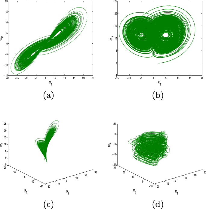

  

  Hyper-chaotic attractors for fractional-order real system (2)

  Fig. 7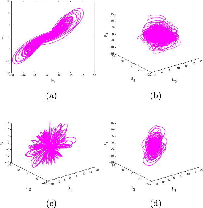

  

  Hyper-chaotic attractors for fractional-order complex system (4)

4 Modulus synchronization scheme

This section discusses the novel synchronization scheme to synchronize real fractional-order hyper-chaotic system and their corresponding complex system.

Consider the master system and slave system in the following form

$$ \begin{array}{@{}rcl@{}} D^{\alpha} U(t)&=& f(U(t)) \end{array} $$

(19)

$$ \begin{array}{@{}rcl@{}} D^{\alpha} W(t)&=& BW(t)+g_{0}(W(t))+C \end{array} $$

(20)

where U(t) = (u₁,u₂,...,u_n)^T denotes the state vector of master system. Note that u is considered as $u=({u_{1}^{r}},{u_{2}^{r}},...,{u_{n}^{r}})^{T}$, $u=({u_{1}^{i}},{u_{2}^{i}},...,{u_{n}^{i}})^{T}$ and $j=\sqrt {-1}$. W(t) = (w₁,w₂,...,w_n)^T are the real state vector of slave system. $A, B\in \mathbb {R}^{N\times N}$ are constant matrix, f,g are n × 1 continuous vector function respectively. C = (C₁,C₂,...,C_n)^T are non-linear controllers which will be designed later. Now, to synchronize complex master system and real slave system, here we define the error system of Modulus synchronization as

$$ e(t)=W(t)-|U(t)| $$

(21)

where |.| denotes the complex modulus of master system.

Definition 1

The synchronization between complex master system and real slave system can be achieved by the following scheme

$$ \lim \| e(t)\|=\lim \| W(t)-| U(t)|\|=0 $$

(22)

where ∥.∥ denotes Euclidean norm and |.| denotes the modulus of complex variable.

Remark 1

If (u^r,uⁱ) = |0,0|, the error can be rewritten as

$$ \begin{array}{@{}rcl@{}} \lim \| e(t)\| &=& \lim \| W(t)-| U(t)|\| \\ &=& \lim \| W-\sqrt{(u^{r})^{2}+(u^{i})^{2}}\|=0 \end{array} $$

Remark 2

If u^r≠ 0 and uⁱ≠ 0, then (22) can be written as

$$ \begin{array}{@{}rcl@{}} \lim \| e(t)\| &=& \lim \| W-\sqrt{(u^{r})^{2}} \| \\ &=& \lim\| W-\vert u^{r}|\|=0 \end{array} $$

(23)

The (23) implies that the synchronization between the complex master system and a real slave system can be turned into an absolute value synchronization problem of real system.

From (22), the error dynamical system can be written as

$$ \begin{array}{@{}rcl@{}} D^{\alpha} e &=& D^{q} W-D^{q}(\sqrt{(u^{r})^{2}+(u^{i})^{2}}) \\ D^{\alpha} e &=& BW(t)+g(V(t))+C-D^{q}(\sqrt{(u^{r})^{2}+(u^{i})^{2}}) \end{array} $$

(24)

The error system can be described as

$$ \begin{array}{@{}rcl@{}} D^{\alpha} e &=& (B-P)e(t) +PW(t)+(B-P)\sqrt{(u^{r})^{2}+(u^{i})^{2}}+g(W(t)) \\ &&-D^{\alpha} \sqrt{(u^{r})^{2}+(u^{i})^{2}} \end{array} $$

(25)

where $P\in \mathbb {R}^{N\times N}$ is a constant control matrix to be chosen.

Theorem 2

If we select the control matrix $P\in \mathbb {R}^{N\times N}$ such that (B − P) is a negative definite matrix, then the complex master system and real slave system are globally synchronized with respect to complex modulus function under the following controllers.

$$ C=-PV(t)-(B-P)\sqrt{(u^{r})^{2}+(u^{i})^{2}}-g(W(t))+D^{\alpha} \sqrt{(u^{r})^{2}+(u^{i})^{2}} $$

(26)

Proof

Using (25) and (26), we get

$$ D^{\alpha} e(t)=(B-P)e(t) $$

(27)

Consider the Lyapunov function as

$$ V(e(t))=\frac{1}{2}e^{T}(t)e(t) $$

We obtain,

$$ D^{\alpha} V(e(t))=D^{q}\left( \frac{1}{2}e^{T}(t)e(t)\right) $$

By using Lemma 1, we get

$$ \begin{array}{@{}rcl@{}} D^{\alpha} V(e(t))\leqslant e^{T}(t)D^{q} e(t) =e^{T}(t)(B-P)e(t) =e^{T}(t)Le(t)<0 \end{array} $$

Thus from the stability theory of Lyapunov, the error system is globally asymptotically stable. Therefore complex master system and real slave system are globally synchronized. □

4.1 Illustration

We consider the complex fractional-order hyper-chaotic system (4) as master system given as follows

$$ \begin{array}{@{}rcl@{}} D^{\alpha}{\mu_{1}} &=& a(\mu_{3}-\mu_{1})+\mu_{3}\mu_{5} \\ D^{\alpha}{\mu_{2}} &=& a(\mu_{4}-\mu_{2})+\mu_{4}\mu_{5} \\ D^{\alpha}{\mu_{3}} &=& b\mu_{3}-\mu_{1}\mu_{5}+\mu_{6} \\ D^{\alpha}{\mu_{4}} &=& b\mu_{4}-\mu_{2}\mu_{5}+\mu_{7} \\ D^{\alpha}{\mu_{5}} &=& -c\mu_{5}+\mu_{1}\mu_{3}+\mu_{2}\mu_{4} \\ D^{\alpha}{\mu_{6}} &=& -d(\mu_{1}+\mu_{3}) \\ D^{\alpha}{\mu_{7}} &=& -d(\mu_{2}+\mu_{4}) \end{array} $$

(28)

Consider the controlled real fractional-order hyper-chaotic system (2) as slave system which is written as

$$ D^{\alpha} W=BW(t)+g_{0}(W(t))+C $$

(29)

where W(t) = (ω₁(t),ω₂(t),ω₃(t),ω₄(t))^T,

$$ B=\begin{bmatrix} -a & a & 0 &0 \\ 0 & -b & 0 & 1 \\ 0 & 0 & -c & 0 \\ -d & -d & 0 & 0\\ \end{bmatrix}, g_{0}(W(t))=\begin{bmatrix} \omega_{2}\omega_{3}\\ -\omega_{1} \omega_{3}\\ \omega_{1} \omega_{2}\\ 0\\ \end{bmatrix} $$

(30)

and C = (C₁,C₂,C₃,C₄) represents a controller.

The error term for modulus synchronization synchronization is defined as

$$ \begin{array}{@{}rcl@{}} e_{1} &=& \omega_{1}-\sqrt{{\mu_{1}^{2}}+{\mu_{2}^{2}}} \\ e_{2} &=& \omega_{2}-\sqrt{{\mu_{3}^{2}}+{\mu_{4}^{2}}} \\ e_{3} &=& \omega_{3}-\mu_{5} \\ e_{4} &=& \omega_{4}-\sqrt{{\mu_{6}^{2}}+{\mu_{7}^{2}}} \end{array} $$

(31)

To achieve modulus synchronization between systems (28) and (29), the control matrix P is chosen as

$$ \begin{bmatrix} 0 & 0 & 0 & 0\\ 0 & 16 & 0 & 0\\ 0 & 0 & 0 & 0\\ -2 & -2 & 0 & 1\\ \end{bmatrix} $$

(32)

The control vector C = (C₁,C₂,C₃,C₄) can be determined as

$$ \begin{array}{@{}rcl@{}} C_{1} &=& 35 \sqrt{{\mu_{1}^{2}}+{\mu_{2}^{2}}}-35\sqrt{{\mu_{1}^{2}}+{\mu_{2}^{2}}}-\omega_{2} \omega_{3}+D^{\alpha}\left( \sqrt{{\mu_{1}^{2}}+{\mu_{2}^{2}}}\right) \\ C_{2} &=& -16 \omega_{2}+\sqrt{{\mu_{3}^{2}}+{\mu_{4}^{2}}}+\omega_{1} \omega_{3}+D^{\alpha}\left( \sqrt{{\mu_{3}^{2}}+{\mu_{4}^{2}}}\right) \\ C_{3} &=& 3 \mu_{5}-\omega_{1} \omega_{2}+D^{\alpha}(\mu_{5}) \\ C_{4} &=& 2 \omega_{1}-2 \omega_{2}-\omega_{4}+D^{\alpha}\left( \sqrt{{\mu_{6}^{2}}+{\mu_{7}^{2}}}\right) \end{array} $$

(33)

The error function can be obtained as

$$ \begin{bmatrix} D^{\alpha} e_{1}\\ D^{\alpha} e_{2}\\ D^{\alpha} e_{3}\\ D^{\alpha} e_{4}\\ \end{bmatrix} =(B-P)* \begin{bmatrix} e_{1}\\ e_{2}\\ e_{3}\\ e_{4}\\ \end{bmatrix} $$

(34)

where

$$ (B-P)= \begin{bmatrix} -30 & 30 & 0 &0 \\ 0 & -1 & 0 & 1 \\ 0 & 0 & -3 & 0\\ 0 & 0 & 0 & -1 \\ \end{bmatrix} $$

(35)

Therefore, it is clear that (B − P) is negative definite matrix. According to Theorem 2, the systems (28) and (29) are globally modulus synchronized with the parameter value are taken as a = 30,b = 15,c = 3 & d = 2 at fractional-order α = 0.95. Figure 8 displays the synchronization error achieved at time t = 4 units (approx.)

Fig. 8

Synchronization error for fractional-order complex system and real system

5 Application of the proposed synchronization scheme

This section applies the synchronized complex and real fractional-order hyper-chaotic systems to develop a new algorithm for digital image encryption and decryption technique. The proposed algorithm has three phases: 1. The key generation phase 2. Encryption phase, and 3. Decryption phase. Before going to construct the algorithm, the following assumptions are needed.

Consider the fractional-order complex system (28) as the sender system and the controlled real fractional-order system (29) as the receiver system. The sender and receiver agree on parameters (t₀,t₁,α,g,p). Figure 8 shows that the modulus synchronization error e(t) between the systems (28) and (29) tends to zero after t ≥ 4 at α = 0.95. So, we fix the parameter values t₀ = 4, t₁ > t₀ and α = 0.95. Further, g is any positive integer less than p where p = 256 since the range of intensity values of an image from 0 to 255.

5.1 Modulus synchronization encryption algorithm

1. Key generation phase:

• 1. The sender chooses a number t₂ > t₀ and solves the system (28) at time t₂. Then computes the private $K_{S_{A}}$ and public key $K_{S_{B}}$ by

  $$ K_{S_{A}}\equiv floor\left( \prod\limits_{i=1}^{7} \mu_{i} (t_{2})\right) * 10^{4} \ (mod\ p) $$
  $$ K_{S_{B}}\equiv g^{K_{S_{A}}} \ (mod\ p) $$

• 2. The sender kept secret their private key $K_{S_{A}}$ and publish the public key $K_{S_{B}}$.

• 3. The receiver chooses a number t₃ > t₀ and solves the system (29) at time t₃. Then computes the private $K_{R_{A}}$ and public key $K_{R_{B}}$ by

  $$ K_{R_{A}}\equiv floor\left( \prod\limits_{i=1}^{4} w_{i} (t_{3})\right) * 10^{4} \ (mod\ p) $$
  $$ K_{R_{B}}\equiv g^{K_{R_{A}}} \ (mod\ p) $$

• 4. The receiver kept secret their private key $K_{R_{A}}$ and publish the public key $K_{R_{B}}$.

2. Encryption phase:

• 5. The sender wants to send a digital image I with size m × n secretly via insecure channel.

• 6. Sender randomly chooses an integer k and calculates T ≡ g^k (mod p) and $s\equiv k+K_{S_{A}} \ (mod\ p)$

• 7. The sender computes an encrypted image E or cipher image of I by

  $$ E\equiv I*\left( K_{R_{B}}^{s} \right)^{-1}* \left( \prod\limits_{i} \phi_{i}(t_{1}) \right)\ (mod\ p) $$

  where $\phi _{1}(t_{1})=floor\left (\sqrt {{\mu _{1}^{2}}(t_{1})+{\mu _{2}^{2}}(t_{1})}\right )$, $\phi _{2}(t_{1})=floor\left (\sqrt {{\mu _{3}^{2}}(t_{1})+{\mu _{4}^{2}}(t_{1})}\right )$, ϕ₃(t₁) = floor(μ₅(t₁)) and $\phi _{4}(t_{1})=floor\left (\sqrt {{\mu _{6}^{2}}(t_{1})+{\mu _{7}^{2}}(t_{1})}\right )$.

• 8. Further, sender sends (T,s,E) to receiver.

3. Decryption phase:

• 9. The receiver receives (T,s,E) from the sender and recovers an original image I or decrypted image D by computing

  $$ I\equiv D\equiv E*(T*K_{S_{B}})^{K_{R_{A}}}*\left( \prod\limits_{i} \psi_{i}(t_{1}) \right)^{-1}\ (mod\ p) $$

  where ψ_i(t₁) = floor(w_i(t₁)),i = 1,2,3,4.

• 10. The validity of the recovered image must be verified by computing $g^{s} \equiv T*K_{S_{B}}\ (mod\ p)$.

For,

$$ \begin{array}{@{}rcl@{}} E*\!(T*K_{S_{B}})^{K_{R_{A}}}*\!\left( \prod\limits_{i} \psi_{i}(t_{1}) \right)^{-1} && \equiv E*(g^{k}*g^{K_{S_{A}}})^{K_{R_{A}}}*\left( \prod\limits_{i} \psi_{i}(t_{1}) \right)^{-1}\ (mod\ p)\\ && \equiv E*\left( g^{kK_{R_{A}}+K_{S_{A}}K_{R_{A}}}\right)*\left( \prod\limits_{i} \psi_{i}(t_{1}) \right)\ (mod\ p)\\ && \equiv I*(K_{R_{B}}^{s})^{-1}* \!\left( \prod\limits_{i} \phi_{i}(t_{1}) \!\right)*\left( g^{kK_{R_{A}}+K_{S_{A}}K_{R_{A}}}\right)*\\ &&\quad \left( \prod\limits_{i} \psi_{i}(t_{1}) \right)^{-1}\ (mod\ p)\\ && \equiv I* \left( K_{R_{B}}^{k+K_{S_{A}}}\right)^{-1}*\left( g^{kK_{R_{A}}+K_{S_{A}}K_{R_{A}}}\right)* \\ &&\quad \left( \prod\limits_{i} \phi_{i}(t_{1}) \right)* \left( \prod\limits_{i} \psi_{i}(t_{1}) \right)^{-1} (mod\ p)\\ && \equiv I* \left( (g^{K_{R_{A}}})^{k+K_{S_{A}}}\right)^{-1}*\left( g^{kK_{R_{A}}+K_{S_{A}}K_{R_{A}}}\right)*\\ &&\quad \left( \prod\limits_{i} \phi_{i}(t_{1}) \right)* \left( \prod\limits_{i} \psi_{i}(t_{1}) \right)^{-1} (mod\ p)\\ && \equiv I* \left( g^{kK_{R_{A}}+K_{S_{A}}K_{R_{A}}}\right)^{-1}*\left( g^{kK_{R_{A}}+K_{S_{A}}K_{R_{A}}}\right)* \\ &&\quad \left( \prod\limits_{i} \phi_{i}(t_{1}) \right)* \left( \prod\limits_{i} \psi_{i}(t_{1}) \right)^{-1} (mod\ p)\\ && \equiv I\ (mod\ p). \end{array} $$

5.2 Demonstration of the proposed algorithm

In this subsection, the performance of the proposed algorithm to be demonstrated experimentally.

Assume that t₁ = 15,t₂ = 10,t₃ = 21,g = 89 and k = 39.

At t₁ = 15, μ₁(t₁) = 2.1639,μ₂(t₁) = 3.0154,μ₃(t₁) = 1.2083,μ₄(t₁) = 1.6837,μ₅(t₁) = 10.5402,μ₆(t₁) = − 4.3571,μ₇(t₁) = − 6.0712 and w₁(t₁) = 3.7115,w₂(t₁) = 2.0724,w₃(t₁) = 10.5402,w₄(t₁) = 7.4729.

At t₂ = 10, μ₁(t₂) = 1.2001,μ₂(t₂) = 1.6754,μ₃(t₂) = 1.0237,μ₄(t₂) = 1.4288,μ₅(t₂) = 8.0642,μ₆(t₂) = − 0.9404,μ₇(t₂) = − 1.3187.

At t₃ = 21, w₁(t₃) = 0.4303,w₂(t₃) = 0.8397,w₃(t₃) = 10.8281,w₄(t₃) = 4.3734.

The private and public keys of sender are

$$ \begin{array}{@{}rcl@{}} K_{S_{A}} && \equiv floor\left( \prod\limits_{i=1}^{7} \mu_{i} (t_{2})\right) * 10^{4} \equiv 208 \ (mod\ 256) \\ K_{S_{B}} && \equiv g^{K_{S_{A}}}\equiv 129 \ (mod\ 256) \end{array} $$

The private and public keys of receiver are

$$ \begin{array}{@{}rcl@{}} K_{R_{A}} && \equiv floor\left( \prod\limits_{i=1}^{4} w_{i} (t_{3})\right) * 10^{4} \equiv 16 \ (mod\ 256) \\ K_{R_{B}} && \equiv g^{K_{R_{A}}}\equiv 129 \ (mod\ 256) \end{array} $$

The sender calculates T ≡ g^k ≡ 169 (mod 256), $s\equiv k+K_{S_{A}}\equiv 247\ (mod\ 256)$ and computes the encrypted image E of an original image I by $E\equiv I*(K_{R_{B}}^{s})^{-1}* \left (\prod \limits _{i} \phi _{i}(t_{1}) \right )\ (mod\ 256)$. Then sends (T,s,E) to receiver. Finally, receiver recovers an original image I by computing $I\equiv D\equiv E*(T*K_{S_{B}})^{K_{R_{A}}}*\left (\prod \limits _{i} \psi _{i}(t_{1}) \right )^{-1}\ (mod\ 256)$

For experiment, we take Coronavirus, Lena, Baboon, Zinnia flowers, Fractal and Autumn leaves images as an original images I and their corresponding encrypted and decrypted images are shown in Fig. 9.

Fig. 9

Left to right from the top: The original, encrypted and decrypted images of Coronavirus, Lena, Baboon, Zinnia flowers, Fractal and Autumn leaves respectively

6 Experimental analysis and comparison results

In this section, the security and performance of the proposed algorithm are analyzed by different security measures.

6.1 Key space analysis

The key space is the total number of different secret keys that can be used in the cryptosystem. A good encryption scheme should have a large key space to resist the brute-force attack. In the proposed image encryption algorithm, the secret keys are the parameters (a,b,c,d) and initial values μ_i(0),i = 1,2,⋯,7, w_i(0),i = 1,2,3,4 of the complex and real fractional-order system, the fractional-order α and the time parameters (t₀,t₁,t₂,t₃). If the computation precision is 10^− 14, then the estimated key space of the proposed algorithm is 10²⁶⁶ ≈ 2⁸⁸⁰. The estimated key space is 8 times greater than the key space size 2¹⁰⁰ to provide the high level security and to resist all varieties of brute-force attacks. The comparison of key space result between the proposed encryption algorithm and the recent existing schemes is given in Table 1.

Table 1 Comparison results of key space

6.2 Information entropy analysis

It is an important analysis to measure the randomness and the unpredictability of an information in the image and the value of the entropy is measured by the following formula

$$ H(s)=-\sum\limits_{i=0}^{2^{N}-1}P(s_{i})\log_{2}P(s_{i}), $$

(36)

where s is the source of information and P(s_i) is the probability of symbol s_i, s_i ∈ s. Theoretically, the maximum entropy value is 8 for a random image with 256 gray levels. A good encryption scheme should produce the entropy value of encrypted image very close to 8 [5, 44]. For the proposed algorithm, the entropy values of encrypted images are listed in Table 2. It is very clear that the entropies of encrypted images are close to 8 and proves that the unpredictability of information is very high. Hence, the proposed encryption algorithm is secure against the entropy analysis and possess good randomness. Further, the comparison result with some existing algorithms is given in Table 3.

Table 2 Information entropy of encrypted images

Table 3 Comparison of information entropy of encrypted images

6.3 Histogram analysis

The histogram reflects the pixel distribution of an image at each intensity level. Figure 10 displays the histograms of the color components of original and encrypted Coronavirus image. It shows that the histogram of encrypted image is entirely different from the original image and it is uniform. Hence, no statistical information about the original image can be observed from the encrypted image.

Fig. 10

Histograms of Red, Green and Blue color components of (a) Coronavirus image and (b) Encrypted Coronavirus image respectively

6.4 Correlation analysis

The efficiency of an encryption algorithm is measured by the correlation of encrypted images. In the good encryption scheme, the correlation coefficient of the encrypted image is close to 0 [5, 44]. That is, the adjacent pixels are entirely uncorrelated to each other. The correlation coefficient between two adjacent pixels in a digital image is calculated by

$$ r_{xy}=\frac{cov(x,y)}{\sqrt{D(x)}\sqrt{D(y)}}, $$

(37)

where $cov(x,y)=\frac {1}{N}\sum \limits _{i=1}^{n} (x_{i}-E(x))(y_{i}-E(y))$, $E(x)=\frac {1}{N}\sum \limits _{i=1}^{n} (x_{i})$ and $D(x)=\frac {1}{N}\sum \limits _{i=1}^{n} (x_{i}-E(x))^{2}$. In the proposed algorithm, the correlation coefficients of two adjacent pixels (2000 pixel pairs are randomly selected) are examined and tabulated in Table 4 for original images and encrypted images in horizontal, vertical, and diagonal directions, respectively. The correlation distribution of the Coronavirus image and their corresponding encrypted image are depicted in Fig. 11. Table 4 shows that the calculated value of correlation coefficients of encrypted images are close to 0 in three different directions, which means the proposed encryption algorithm is secure well and robust against correlation attacks. Further, the effectiveness of the proposed algorithm is satisfactory when compared with other existing encryption algorithms presented in Table 5.

Table 4 Correlation coefficients of two adjacent pixels in original and encrypted images

Fig. 11

Correlation distributions between two adjacent pixels: (a) Horizontal, (b) Vertical (c) Diagonal directions in Coronavirus image and (a1) Horizontal, (b1) Vertical (c1) Diagonal directions in encrypted Coronavirus image respectively

Table 5 Comparison of correlation coefficients of two adjacent pixels in different directions

Remark 3

The results of experiments and their corresponding security analysis show that the security of the proposed modulus synchronization encryption algorithm is very high, has a huge key space size, and is secure against different attacks.

7 Conclusions

This paper investigates the dynamical behaviors of the proposed fractional-order real and complex hyper-chaotic systems. The modulus synchronization scheme has been suggested for fractional-order hyper-chaotic complex and real systems by using non-linear controllers. Necessary and sufficient conditions are derived from achieving the proposed synchronization and verified by numerical simulations. A novel modulus synchronization encryption algorithm with a large key space for digital images has been proposed and demonstrated numerically. Several tests have carried out the security and performance analysis of the proposed algorithm. The obtained results prove that the proposed image encryption algorithm has better performance than existing algorithms. Experimental results show that the proposed encryption algorithm is suitable to protect the security of digital image information. In future work, a novel encryption algorithm with higher level security will be constructed based on fractional order dynamical systems to protect the medical image information over the internet.

References

Aguila-Camacho N, Duarte-Mermoud MA, Gallegos JA (2014) Lyapunov functions for fractional order systems. Commun Nonlinear Sci Numer Simul 19(9):2951–2957
Bagley RL, Calico R (1991) Fractional order state equations for the control of viscoelasticallydamped structures. Journal of Guidance. Control, and Dynamics 14(2):304–311
Balasubramaniam P, Muthukumar P, Ratnavelu K (2015) Theoretical and practical applications of fuzzy fractional integral sliding mode control for fractional-order dynamical system. Nonlinear Dyn 80(1-2):249–267
Bansal M, Kumar M (2021) Kumar, m.: 2d object recognition techniques: state-of-the-art work. Archives of Computational Methods in Engineering 28(3):1147–1161
Brindha M, Gounden NA (2016) A chaos based image encryption and lossless compression algorithm using hash table and chinese remainder theorem. Appl Soft Comput 40:379–390
Butzer PL, Westphal U (2000) An introduction to fractional calculus Applications of fractional calculus in physics, pp 1–85. World scientific
Chen L, Chai Y, Wu R, Sun J, Ma T (2012) Cluster synchronization in fractional-order complex dynamical networks. Phys Lett A 376(35):2381–2388
Chua L, Komuro M, Matsumoto T (1986) The double scroll family. IEEE transactions on circuits and systems 33(11):1072–1118
Dargan S, Kumar M, Ayyagari MR, Kumar G (2020) A survey of deep learning and its applications: a new paradigm to machine learning. Archives of Computational Methods in Engineering 27(4):1071–1092
Garg D, Garg NK, Kumar M (2018) Underwater image enhancement using blending of clahe and percentile methodologies. Multimed Tools Appl 77 (20):26,545–26,561
Gholamin P, Sheikhani AR (2019) Dynamical analysis of a new three-dimensional fractional chaotic system. Pramana 92(6):91
Gupta S, Kumar M (2020) Forensic document examination system using boosting and bagging methodologies. Soft Comput 24(7):5409–5426
Gupta S, Mohan N, Kumar M (2021) A study on source device attribution using still images. Archives Computat Methods Eng 28(4):2209–2223
HE JB, WU ZX, YU YL, LI XJ (2013) A mthod of video encryption communication based on fractional hyperchaotic chen system [j]. J Zhangzhou Normal Univ (Natural Sci), vol 2
Hasanzadeh E, Yaghoobi M (2019) A novel color image encryption algorithm based on substitution box and hyper-chaotic system with fractal keys. Multimed Tools Appl:1–19
Huang Y, Huang L, Wang Y, Peng Y, Yu F (2020) Shape synchronization in driver-response of 4-d chaotic system and its application in image encryption. IEEE Access 8:135,308–135,319
Kayalvizhi S, Malarvizhi S (2020) A novel encrypted compressive sensing of images based on fractional order hyper chaotic chen system and dna operations. Multimed Tools Appl 79(5):3957–3974
Khan A, Jahanzaib LS et al (2019) Synchronization on the adaptive sliding mode controller for fractional order complex chaotic systems with uncertainty and disturbances. Inte J Dynamics Contr 7(4):1419–1433
Khan A, Khan N (2021) A novel finite-time terminal observer of a fractional-order chaotic system with chaos entanglement function. Math Methods Appl Sci
Khan N, Muthukumar P (2021) Transient chaos, synchronization and digital image enhancement technique based on a novel 5d fractional-order hyperchaotic memristive system. Circuits Syst Signal Process:1–24
Khan A et al (2021) A comparative study between two different adaptive sliding mode control techniques. Int J Appl Computat Math 7(4):1–18
Kumar M, Gupta S, Mohan N (2020) A computational approach for printed document forensics using surf and orb features. Soft Comput 24 (17):13,197–13,208
Li P, Du J, Li S, Zheng Y (2019) Modulus synchronization of a novel hyperchaotic real system and its corresponding complex system. IEEE Access 7:109,577–109,584
Li Z, Xia T, Jiang C (2019) Synchronization of fractional-order complex chaotic systems based on observers. Entropy 21(5):481
Li P, Xu J, Mou J, Yang F (2019) Fractional-order 4d hyperchaotic memristive system and application in color image encryption. EURASIP J Image Video Process 2019(1):22
Li T, Yang M, Wu J, Jing X (2017) A novel image encryption algorithm based on a fractional-order hyperchaotic system and dna computing. Complexity, vol 2017
Lien C, Vaidyanathan S, Zhang S, Sambas A et al (2019) A hyperchaotic system with three quadratic nonlinearities, its dynamical analysis and circuit realization. In: Journal of physics: conference series. IOP publishing, vol 1179, p 012085
Luo C, Wang X (2013) Chaos generated from the fractional-order complex chen system and its application to digital secure communication. Int J Modern Phys C 24(04):1350,025
Luo C, Wang X (2013) Chaos in the fractional-order complex lorenz system and its synchronization. Nonlinear Dyn 71(1-2):241–257
Mohadeszadeh M, Karimpour A, Pariz N (2019) Synchronisation of fractional-order complex systems and its application. Pramana 92(2):29
Muthukumar P, Balasubramaniam P, Ratnavelu K (2014) Synchronization and an application of a novel fractional order king cobra chaotic system. Chaos: an Interdisciplinary J Nonlinear Sci 24(3):033,105
Muthukumar P, Balasubramaniam P, Ratnavelu K (2014) Synchronization of a novel fractional order stretch-twist-fold (stf) flow chaotic system and its application to a new authenticated encryption scheme (aes). Nonlinear Dyn 77(4):1547–1559
Muthukumar P, Balasubramaniam P, Ratnavelu K (2018) Sliding mode control for generalized robust synchronization of mismatched fractional order dynamical systems and its application to secure transmission of voice messages. ISA Trans 82:51–61
Niu Y, Sun X, Zhang C, Liu H (2020) Anticontrol of a fractional-order chaotic system and its application in color image encryption. Math Probl Eng, vol 2020
Podlubny I (1998) Fractional differential equations: an introduction to fractional derivatives, fractional differential equations, to methods of their solution and some of their applications, vol 198. Elsevier
Saichev AI, Zaslavsky GM (1997) Fractional kinetic equations: solutions and applications. Chaos Interdisciplinary J Nonlinear Sci 7(4):753–764
Tavazoei MS, Haeri M (2007) A necessary condition for double scroll attractor existence in fractional-order systems. Phys Lett A 367(1-2):102–113
Yadav VK, Kumar R, Leung A, Das S (2019) Dual phase and dual anti-phase synchronization of fractional order chaotic systems in real and complex variables with uncertainties. Chinese J Phys 57:282–308
Yadav VK, Srikanth N, Das S (2016) Dual function projective synchronization of fractional order complex chaotic systems. Optik 127(22):10,527–10,538
Yang YG, Guan BW, Zhou YH, Shi WM (2020) Double image compression-encryption algorithm based on fractional order hyper chaotic system and dna approach. Multimed Tools Appl:1–20
Yang F, Mou J, Sun K, Cao Y, Jin J (2019) Color image compression-encryption algorithm based on fractional-order memristor chaotic circuit. IEEE Access 7:58,751–58,763
Zhang YQ, Hao JL, Wang XY (2020) An efficient image encryption scheme based on s-boxes and fractional-order differential logistic map. IEEE Access 8:54,175–54,188
Zhang LM, Sun KH, Liu WH, He SB (2017) A novel color image encryption scheme using fractional-order hyperchaotic system and dna sequence operations. Chin Phys B 26(10):100,504
Zhu S, Wang G, Zhu C (2019) A secure and fast image encryption scheme based on double chaotic s-boxes. Entropy 21(8):790
Acknowledgements
Nasreen(19/06/2016(i)EU-V) thankful to UGC,India for providing financial support as S.R.F.
Author information
Authors and Affiliations
Corresponding author
Ethics declarations
Conflict of Interests
The authors declare that they have no conflict of interest.
Additional information
Publisher’s note
Springer Nature remains neutral with regard to jurisdictional claims in published maps and institutional affiliations.
Rights and permissions
Springer Nature or its licensor holds exclusive rights to this article under a publishing agreement with the author(s) or other rightsholder(s); author self-archiving of the accepted manuscript version of this article is solely governed by the terms of such publishing agreement and applicable law.
About this article
Cite this article
Muthukumar, P., Khan, N. The large key space image encryption algorithm based on modulus synchronization between real and complex fractional-order dynamical systems. Multimed Tools Appl 82, 17801–17825 (2023). https://doi.org/10.1007/s11042-022-14074-6
Received:
Revised:
Accepted:
Published:
Issue Date:
DOI: https://doi.org/10.1007/s11042-022-14074-6