
Abstract
We consider rough differential equations whose coefficients contain path-dependent bounded variation terms and prove the existence and a priori estimate of solutions. These equations include classical path-dependent stochastic differential equations containing running maximum processes and normal reflection terms. We apply these results to determine the topological support of the solution processes.
1 Introduction
In the framework of Itô’s calculus, path-dependent stochastic differential equations(=SDEs) are naturally formulated and the existence and uniqueness hold under suitable standard assumptions on the coefficients. For example, reflected SDEs and SDEs containing running maximum and minimum processes are typical examples. In one dimensional cases, very simple SDEs containing the maximum and minimum processes and reflection term have been studied in detail. In this paper, we consider rough differential equations (=RDEs) whose coefficients contain path-dependent bounded variation terms and prove the existence and a priori estimate of solutions. This class of equations include the classical path-dependent SDEs mentioned above. Although the solutions are not unique in general, the uniqueness holds for smooth rough paths in many cases. Under the uniqueness assumption, we prove a continuity property of solution mappings at smooth rough paths which is useful to determine the topological support of the solution processes.
The structure of this paper is as follows. In Sect. 2, we introduce a class of RDEs containing bounded variation terms:
where \(\textbf{X}_t\) is a \(1/\beta \) rough path (\(1/3<\beta \le 1/2\)) and \(A(Z)_t\) is a continuous bounded variation path which depends on the past path \((Z_s)_{s\le t}\). After that, we state our main theorem (Theorem 2.7) which proves the existence and a priori estimate of solutions under \(\sigma \in \textrm{Lip}^{\gamma -1}\) (\(\gamma >1/\beta \)) and suitable assumptions on A. Note that the regularity assumption on \(\sigma \) for the existence of solutions is standard in the case of usual RDEs which corresponds to \(A\equiv 0\). The solution \(Z_t\) is a controlled path of the driving rough path \(\textbf{X}\). Actually, we solve this equation in product Banach spaces consisting of Z and \(\Psi =A(Z)\) by applying Schauder’s fixed point theorem.
To this end, we introduce Hölder continuous path spaces \(\mathcal {C}^{\theta }\) and Banach spaces \(\mathcal {C}^{q\text {-}var, \theta }\) consisting of \(\Psi \) based on the control function \(\omega \) of \(\textbf{X}\). The latter is a set of paths whose q-variation norms \((q\ge 1)\) are finite and satisfy a certain Hölder continuity defined by \(\omega \). We also study basic properties of the functional A. We briefly explain examples but we will discuss the detail in Sect. 5.
In Sect. 3, we prove our main theorem. The uniqueness does not hold in general. See Remark 2.8 (6).
In Sect. 4, we consider usual \(\beta \)-Hölder rough path \(\textbf{X}\) with the control function \(\omega (s,t)=|t-s|\). We show that the (generally multivalued) solution mapping is continuous at a rough path for which the solution is unique in Proposition 4.2 using a priori estimate of solutions. We use this result to prove support theorems in Sect. 6.
In Sect. 5, we give examples. In Sect. 5.1, we consider reflected rough differential equations on a domain D in \({\mathbb R}^n\):
where \(\Phi _t\) is the reflection term which forces \(Y_t\in \bar{D}\). This equation looks different from the equation studied in the main theorem. However, it is well-known that reflected Itô (Stratonovich) SDEs can be transformed to certain path-dependent Itô (Stratonovich) SDEs without reflection term. This is used to prove Freidlin-Wentzell type large deviation principle ([5]) and the support theorem ([14]) for reflected diffusions on domains with smooth boundary. We prove the existence theorem (Theorem 5.6) under standard assumptions (A) and (B) on D and \(\sigma \in \textrm{Lip}^{\gamma -1}\) by transforming the Eq. (1.2) to the corresponding path-dependent RDE (1.1). This is an extension of the result in [2] in which we proved the existence of solutions of (1.2) under stronger assumptions that D satisfies the condition (H1) and \(\sigma \in C^3_b\).
In 1-dimensional cases, perturbed SDEs and perturbed reflected SDEs were studied by many people. See e.g. [7, 8, 10, 11, 13, 31, 36]. In Sect. 5.2, we give a short review of these subjects.
In Sect. 5.3, we consider multidimensional and rough path versions of 1-dimensional perturbed SDEs and perturbed reflected SDEs. In the study of the latter one, we need to consider an implicit Skorohod equation as in [2]. As for perturbed reflected SDE whose driving process is the standard Brownian motion, we can extend the existence and uniqueness result of the solution due to Doney and Zhang [13] by using our approach. See Remark 5.22.
Path-dependent functional \(A(x)_t\) which we are mainly concerned with in this paper is a kind of generalization of the maximum process \(\max _{0\le s\le t}|x_s|\) and the local time term \(L(x)_t\). The maximum process \(\max _{0\le s\le t}|x_s|\) is obtained as the limit of \(\Vert x\Vert _{L^p([0,t])}\) as \(p\rightarrow \infty \). Hence it may be natural to study the case where \(A(x)_t=\Vert x\Vert _{L^p([0,t])}\). In Sect. 5.4, we study such examples.
In Sect. 6, we prove support theorems for solution processes by using Proposition 4.2 and Wong–Zakai theorems. In this section, except Theorem 6.4, we consider the Brownian rough path \(\textbf{W}\) which implies that we consider the usual Stratonovich SDEs driven by the standard Brownian motion.
Section 1 is an appendix. The solution \(Y_t\) studied in Sect. 5 is a sum of a controlled path \(Z_t\) and a continuous bounded variation path \(\Phi _t\). For a given controlled path Z, the Gubinelli derivative \(Z'\) is uniquely determined if the first level path X of \(\textbf{X}\) is truly rough in the sense of [20]. In our case, \(\Phi \) is certainly bounded variation but does not have good regularity property in Hölder norm. Hence it is natural to ask whether \(Z'\) is unique or not for Y in our setting. We study this problem by using a certain rough property of the path X in Sect. 7.1. In Sect. 7.2, we make a remark on path-dependent rough differential equations with drift. This consideration is necessary for the study of the reflected diffusions with the drift terms.
2 Preliminary and Main Theorem
Let us fix a positive number T. Let \(\omega (s,t)\) \((0\le s\le t\le T)\) be a control function. That is, \((s,t)\mapsto \omega (s,t)\in {\mathbb R}^{+}\) is a continuous function and \(\omega (s,u)+\omega (u,t)\le \omega (s,t)\) \((0\le s\le u\le t\le T)\) holds. We introduce a mixed norm by using \(\omega \) and p-variation norm. We refer the readers to [21] for the related studies. Let E be a finite dimensional normed linear space. For a continuous path \((x_t)\) \((0\le t\le T)\) on E, we define for \([s,t]\subset [0,T]\),
where \(\mathcal{P}=\{s=t_0<\cdots <t_N=t\}\) is a partition of the interval [s, t] and \(x_{u,v}=x_v-x_u\). When \([s,t]=[0,T]\), we may omit denoting [0, T]. For \(0<\theta \le 1, q\ge 1\), \(0\le s\le t\le T\) and a continuous path x, we define
We use the convention that \(\inf \emptyset =+\infty \). When \(\omega (s,t)=|t-s|\), \(\Vert x\Vert _{\theta , [s,t]}<\infty \) is equivalent to that \(x_u\) \((s\le u\le t)\) is a Hölder continuous path with the exponent \(\theta \) in usual sense. Hence we may say x is an \(\omega \)-Hölder continuous path with the exponent \(\theta \) (\((\omega ,\theta )\)-Hölder continuous path in short). For two parameter function \(F_{s,t}\) \((0\le s\le t\le T)\), we define \(\Vert F\Vert _{\theta ,[s,t]}\) similarly.
We denote by \(\mathcal {C}^{\theta }([0,T], E)\) the set of \(\omega \)-Hölder continuous paths x with values in E satisfying \(\Vert x\Vert _{\theta }=\Vert x\Vert _{\theta ,[0,T]}<\infty \). We may denote the function space by \((\mathcal {C}^{\theta }([0,T], E),\omega )\) to specify the control function. \(\mathcal {C}^{\theta }([0,T], E)\) is a Banach space with the norm \(|x_0|+\Vert x\Vert _{\theta }\). We may just write \(\mathcal {C}^{\theta }(E)\) if there is no confusion. Let \(\mathcal {C}^{q\text {-}var,\theta }(E)\) denote the set of E-valued continuous paths of finite q-variation defined on [0, T] satisfying \(\Vert x\Vert _{q\text {-}var,\theta }:=\Vert x\Vert _{q\text {-}var,\theta ,[0,T]}<\infty \). Note that \(\mathcal {C}^{q\text {-}var,\theta }(E)\) is a Banach space with the norm \(|x_0|+\Vert x\Vert _{q\text {-}var,\theta }\). Obviously, any path \(x\in \mathcal {C}^{q\text {-}var,\theta }(E)\) satisfy \(|x_{s,t}|\le \Vert x\Vert _{q\text {-}var,\theta }\omega (s,t)^{\theta }\). We may write \(\mathcal {C}^{\theta }, \mathcal {C}^{q\text {-}var,\theta }\) for simplicity.
We next introduce the notation for mappings between normed linear spaces. Let E, F be finite dimensional normed linear spaces. For \(\gamma =n+\theta \) \((n\in {\mathbb N}\cup \{0\}, 0<\theta \le 1)\), \(\textrm{Lip}^{\gamma }(E,F)\) denotes the set of bounded functions f on E with values in F which are n-times continuously differentiable and whose derivatives up to n-th order are bounded and \(D^nf\) is a Hölder continuous function with the exponent \(\theta \) in usual sense.
We use the following lemma. The compact embedding in (2) is necessary for the application of the Schauder fixed point theorem.
Lemma 2.1
-
(1)
Let \(1\le q'\le q\). For a continuous path x, we have
$$\begin{aligned} \Vert x\Vert _{q\text {-}var,[s,t]}\le \Vert x\Vert _{q'\text {-}var,[s,t]}^{q'/q} \Vert x\Vert _{\infty \text {-}var,[s,t]}^{(q-q')/q} \le \Vert x\Vert _{q'\text {-}var,[s,t]}. \end{aligned}$$(2.6) -
(2)
Let \(1\le q'\le q\). Let \(0<\theta , \theta '\le 1\) be positive numbers such that \(q\theta \le q'\theta '\). Then for any \(x\in \mathcal {C}^{q'\text {-}var,\theta '}\), we have
$$\begin{aligned} \Vert x\Vert _{q\text {-}var,\theta }\le \omega (0,T)^{(q'\theta '-q\theta )/q} \Vert x\Vert _{q'\text {-}var,\theta '}^{q'/q} \Vert x\Vert _{\infty \text {-}var}^{(q-q')/q}. \end{aligned}$$(2.7)Further if \(q'<q\) holds, then the inclusion \(\mathcal {C}^{q'\text {-}var,\theta '}\subset \mathcal {C}^{q\text {-}var,\theta }\) is compact.
-
(3)
If \(\Vert x\Vert _{q\text {-}var,[s,t]}<\infty \) for some q, then \(\lim _{q\rightarrow \infty }\Vert x\Vert _{q\text {-}var,[s,t]}=\Vert x\Vert _{\infty \text {-}var,[s,t]}\).
Proof
(1) We have
The second inequality follows from the trivial bound \(\Vert x\Vert _{\infty \text {-}var,[s,t]}\le \Vert x\Vert _{q'\text {-}var,[s,t]}\).
(2) By (1), we have
This implies (2.7). If \(\sup _n|(x_n)_0|+\Vert x_n\Vert _{q'\text {-}var,\theta '}<\infty \), then by their equicontinuities, there exists a subsequence such that \(x_{n_k}\) converges to a certain function \(x_{\infty }\) in the uniform norm. By (2.7), we can conclude that the convergence takes place with respect to the norm on \(\mathcal {C}^{q\text {-}var,\theta }\).
(3) We need only to prove \(\limsup _{q\rightarrow \infty }\Vert x\Vert _{q\text {-}var,[s,t]}\le \Vert x\Vert _{\infty \text {-}var,[s,t]}\). Suppose \(\Vert x\Vert _{q_0\text {-}var,[s,t]}<\infty \). Then for \(q>q_0\),
Taking the limit \(q\rightarrow \infty \), we obtain the desired estimate. \(\square \)
Throughout this paper, \(\beta \) is a positive number satisfying \(1/3<\beta \le 1/2\) if there are no further comments. Let \(\omega \) be a control function and let \(\textbf{X}_{s,t}=(X_{s,t},{\mathbb X}_{s,t})\) \((0\le s\le t\le T)\) be a \((\omega ,\beta )\)-Hölder rough path on \({\mathbb R}^d\). That is, \(\textbf{X}\) satisfies Chen’s relation and the path regularity conditions,
where \(\Vert X\Vert _{\beta }(<\infty )\) and \(\Vert {\mathbb X}\Vert _{2\beta }(<\infty )\) denote the \(\omega \)-Hölder norm. We denote by \(\mathscr {C}^{\beta }({\mathbb R}^d)\) the set of all \((\omega ,\beta )\)-Hölder rough paths, where \(\omega \) moves in the set of all control functions. When \(\omega (s,t)=|t-s|\), \(\textbf{X}_{s,t}\) is a usual \(\beta \)-Hölder rough path. If \(\textbf{X}_{s,t}\) is a rough path with finite \(1/\beta \)-variation, setting \(\omega (s,t)=\Vert X\Vert _{1/\beta \text {-}var, [s,t]}^{1/\beta }+ \Vert {\mathbb X}\Vert _{1/(2\beta )\text {-}var, [s,t]}^{1/(2\beta )}\), \(\Vert X\Vert _{\beta }\le 1\) and \(\Vert {\mathbb X}\Vert _{2\beta }\le 1\) hold. We refer the reader to [6, 20, 22, 28, 29] for the references of rough paths.
We use the following quantity,

We introduce a set of controlled paths \({\mathscr {D}}^{2\theta }_X({\mathbb R}^n)\) of \(\textbf{X}_{s,t}\), where \(1/3<\theta \le \beta \) following [20, 24]. A pair of \(\omega \)-Hölder continuous paths \((Z,Z')\in \mathcal {C}^{\theta }([0,T],{\mathbb R}^n)\times \mathcal {C}^{\theta }([0,T], \mathcal{L}({\mathbb R}^d,{\mathbb R}^n))\) with the exponent \(\theta \) is called a controlled path of X, if the remainder term \(R^Z_{s,t}=Z_t-Z_s-Z'_sX_{s,t}\) satisfies \(\Vert R^Z\Vert _{2\theta }<\infty \). The set of controlled paths \({\mathscr {D}}^{2\theta }_X({\mathbb R}^n)\) is a Banach space with the norm
The rough differential equations which we will study contain path dependent bounded variation term \(A(x)_t\). We consider the following condition on A. Note that the function space \(\mathcal {C}^{\beta }\) in the following statement depends on the control function \(\omega \).
Assumption 2.2
Let \(\xi \in {\mathbb R}^n\). Let \(\omega \) be a control function. Let A be a mapping from \(\mathcal {C}^{\beta }([0,T], {\mathbb R}^n~|~x_0=\xi )\) to \(C([0,T], {\mathbb R}^n)\) satisfying the following.
-
(1)
\((\text {Adaptedness})\) \(\left( A(x)_s\right) _{0\le s\le t}\) depends only on \((x_s)_{0\le s\le t}\) for all \(0\le t\le T\).
-
(2)
\((\text {Continuity})\) There exists \(1/3<\beta _0<\beta \) such that A can be extended to a continuous mapping from \(\mathcal {C}^{\beta _0}([0,T],{\mathbb R}^n~|~x_0=\xi )\) to \((C([0,T], {\mathbb R}^n), \Vert ~\Vert _{\infty ,[0,T]})\). We use the same notation A to denote the extended mapping on \(\mathcal {C}^{\beta _0}\).
-
(3)
There exists a non-decreasing positive continuous function F on \([0,\infty )\) such that for all \(x\in \mathcal {C}^{\beta _0}([0,T],{\mathbb R}^n~|~x_0=\xi )\),
$$\begin{aligned} \Vert A(x)\Vert _{1\text {-}var,[s,t]}\le F(\Vert x\Vert _{(1/\beta _0)\text {-}var,[s,t]}) \Vert x\Vert _{\infty \text {-}var,[s,t]}, \quad 0\le s\le t\le T \nonumber \\ \end{aligned}$$(2.14)hold.
Remark 2.3
The conditions (1), (2) are natural. In many cases, A is defined on continuous path spaces and is continuous with respect to the uniform norm. The condition (3) is strong assumption. This implies that the total variation of A(x) on [s, t] can be estimated by the norm of the path \((x_u-x_s)\) on \(s\le u\le t\). Note that this does not exclude the case where \(A(x)_u\) \((s\le u\le t)\) depends on \(x_v\) \((v\le s)\).
We have the following simple result.
Lemma 2.4
Let \(\omega \) be a control function and let \(\mathcal {C}^{\beta }([0,T],{\mathbb R}^n)\) be the corresponding Hölder space.
-
(1)
Suppose \(A: \mathcal {C}^{\beta }([0,T], {\mathbb R}^n~|~x_0=\xi )\rightarrow C([0,T], {\mathbb R}^n)\) satisfies Assumption 2.2 (1), (2). Then the initial value \(A(x)_0\) is independent of \(x\in \mathcal {C}^{\beta }([0,T], {\mathbb R}^n~|~x_0=\xi )\).
-
(2)
Let \(0<T'<T\) and set \(\omega _{T'}(s,t)=\omega (T'+s,T'+t)\) \((0\le s\le t\le T-T')\). Then \(\omega _{T'}\) is a control function.
-
(3)
Let \(\mathcal {C}^{\beta }_{T'}([0,T-T'],{\mathbb R}^n)\) be the \((\omega _{T'},\beta )\)- Hölder space. Let \(y\in \mathcal {C}^{\beta }([0,T'],{\mathbb R}^n)\) and \(x\in \mathcal {C}^{\beta }_{T'}([0,T-T'],{\mathbb R}^n)\) and suppose \(y_{T'}=x_0\). Set
$$\begin{aligned} \tilde{x}_t= {\left\{ \begin{array}{ll} y_t &{} t\le T',\\ x_{t-T'} &{}T'\le t\le T. \end{array}\right. } \end{aligned}$$Then \(\tilde{x}\in \mathcal {C}^{\beta }([0,T],{\mathbb R}^n)\). Let
$$\begin{aligned} \tilde{A}_{y,T'}(x)_t=A(\tilde{x})_{T'+t},\quad 0\le t\le T-T',\quad x\in \mathcal {C}^{\beta }_{T'}([0,T-T'],{\mathbb R}^n~|~x_0=y_{T'}). \end{aligned}$$Then \(\tilde{A}_{y,T'}\) satisfies Assumption 2.2 replacing \(\omega \) and T by \(\omega _{T'}\) and \(T-T'\). In particular, (2.14) holds for the same function F.
Proof
(1) For \(x\in C([0,T],{\mathbb R}^n)\), let \(x^t_u=x_{t\wedge u}\). Then by Assumption 2.2 (1), \(A(x)_u=A(x^t)_u\) \((0\le u\le t)\) holds. By a simple calculation, for any \(x,y\in C([0,T],{\mathbb R}^n)\), we have
Since \((y^0)^t=y^0\), this implies \(\lim _{t\rightarrow +0}\Vert x^t-y^0\Vert _{\mathcal {C}^{\beta _0}}=0\). Hence
(2) and (3) are easy to check. \(\square \)
Actually, the condition (3) automatically implies the following stronger estimate. By this result, we may assume that the growth rate of F(u) is at most of order \(u^{1/\beta }\), that is, a polynomial order.
Lemma 2.5
Assume the mapping \(A: \mathcal {C}^{\beta }([0,T], {\mathbb R}^n~|~x_0=\xi ) \rightarrow C([0,T], {\mathbb R}^n)\) satisfies the condition (3) in Assumption 2.2.
-
(1)
There exists \(C>0\) such that
$$\begin{aligned} \Vert A(x)\Vert _{1\text {-}var,[s,t]}\le C\left( \Vert x\Vert _{(1/\beta _0)\text {-}var, [s,t]}^{1/\beta _0}+1\right) \Vert x\Vert _{\infty \text {-}var,[s,t]} \quad 0\le s\le t\le T. \end{aligned}$$(2.15) -
(2)
Let us choose positive numbers \(\tilde{\alpha }\) and q such that \(\tilde{\alpha }\le \beta \) and \(1\le q\le \beta /\tilde{\alpha }\). Then for any \(x,x'\in \mathcal {C}^{\beta }\), we have
$$\begin{aligned}&\Vert A(x)-A(x')\Vert _{q\text {-}var, \tilde{\alpha }}\nonumber \\&\le \omega (0,T)^{\frac{\beta }{q}-\tilde{\alpha }} \left( F(\Vert x\Vert _{\beta _0}\omega (0,T)^{\beta _0}) \Vert x\Vert _{\beta }+ F(\Vert x'\Vert _{\beta _0}\omega (0,T)^{\beta _0}) \Vert x'\Vert _{\beta } \right) ^{1/q}\nonumber \\&\qquad \qquad \times \Vert A(x)-A(x')\Vert _{\infty \text {-}var}^{1-(1/q)}. \end{aligned}$$(2.16)
Proof
Let \( \omega _{1/\beta _0}(s,t)=\Vert x\Vert _{1/\beta _0\text {-}var, [s,t]}^{1/\beta _0}. \) For \(\varepsilon >0\), we choose the points \(s=t_0<t_1<\cdots <t_N=t\) such that \(\omega _{1/\beta _0}(t_{i-1},t_i)=\varepsilon \) \((1\le i\le N-1)\) and \(\omega _{1/\beta _0}(t_{N-1},t_N)\le \varepsilon \). By the super additivity of \(\omega _{1/\beta _0}\), we have \( (N-1)\varepsilon \le \sum _{i=1}^N\omega _{1/\beta _0}(t_{i-1},t_i)\le \omega _{1/\beta _0}(s,t) \) and \(N\le \omega _{1/\beta _0}(s,t)/\varepsilon +1\). By the additivity property of the bounded variation norm, we have
which implies the desired estimate.
(2) Applying Lemma 2.1 (2) in the case where \(q'=1, \theta '=\beta , \theta =\tilde{\alpha }\), we have
Note that
By the assumption on A, we have
This completes the proof. \(\square \)
Remark 2.6
Of course, we may optimize the estimate (2.15) as follows:
where \(\tilde{F}(u)=\inf _{\varepsilon >0}F(\varepsilon )\left\{ \left( \frac{u}{\varepsilon }\right) ^{1/\beta _0}+1\right\} \).
We now introduce our RDEs and state our main theorem.
Theorem 2.7
Let \(\gamma >1/\beta \). Let \(\textbf{X}\) be a \((\omega ,\beta )\)-Hölder rough path. Let \(\sigma \in \textrm{Lip}^{\gamma -1}({\mathbb R}^n\times {\mathbb R}^n, \mathcal{L}({\mathbb R}^d,{\mathbb R}^n))\) and \(\xi \in {\mathbb R}^n\). Assume that the mapping \(A: \mathcal {C}^{\beta }([0,T], {\mathbb R}^n~|~x_0=\xi ) \rightarrow C([0,T], {\mathbb R}^n)\) satisfies the condition in Assumption 2.2. Then the following hold.
-
(1)
There exists a controlled path \((Z,Z')\in {\mathscr {D}}^{2\beta }_X({\mathbb R}^n)\) such that
$$\begin{aligned} Z_t&=\xi +\int _0^t\sigma (Z_s,A(Z)_s)d\textbf{X}_s,\quad Z'_t=\sigma (Z_t,A(Z)_t),\quad 0\le t\le T. \end{aligned}$$(2.20) -
(2)
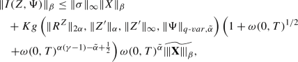
All solutions \((Z,Z')\) of (2.20) satisfy the following estimate: there exist positive constants K and \(\kappa _1,\kappa _2,\kappa _3\) which depend only on \(\sigma , \beta , \gamma \), F such that
 (2.21)

First we make some remarks for this theorem and after that we explain some examples.
Remark 2.8
(1) From now on, we always set \(\gamma >1/\beta \) for \(1/3<\beta \le 1/2\) if there is no further comment.
(2) Let \((Z,Z')\in {\mathscr {D}}^{2\theta }_X({\mathbb R}^n)\) \((1/3<\theta \le \beta )\). Let \(\{\Psi _t\}_{0\le t\le T}\) be a continuous bounded variation path on \({\mathbb R}^n\). Then we can define the integral \(\int _0^t\sigma (Z_s, \Psi _s)d\textbf{X}_s\) in a similar way to the usual rough integral. We denote the derivative of \(\sigma =\sigma (\xi ,\eta )\) \((\xi \in {\mathbb R}^n, \eta \in {\mathbb R}^n)\) with respect to \(\xi \) by \(D_1\sigma \) and \(\eta \) by \(D_2\sigma \). Let
and \(\tilde{\Xi }^{\Psi }_{s,t}=\Xi ^{\Psi }_{s,t} -(D_2\sigma )(Z_s,\Psi _s)\int _s^t\Psi _{s,r}\otimes dX_r\). Let \(\mathcal{P}=\{s=t_0<\cdots <t_N=t\}\) and write \(|\mathcal{P}|=\max _i|t_{i+1}-t_i|\). Then it is easy to check that \(\lim _{|\mathcal{P}|\rightarrow 0}\sum _{i=1}^N \Xi ^{\Psi }_{t_{i-1},t_i}\) converges by the Sewing lemma using (3.8). Actually \(\lim _{|\mathcal{P}|\rightarrow 0}\sum _{i=1}^{N} \tilde{\Xi }^{\Psi }_{t_{i-1},t_i}\) also converges to the same limit value. We denote the limit by \(\int _s^t\sigma (Z_u,\Psi _u)d\textbf{X}_u\). Hence the sum of the term \(\int _s^t\Psi _{s,r}\otimes dX_r\) does not have any effect on the integral. However, we need to consider \(\Xi ^{\Psi }\) instead of \(\tilde{\Xi }^{\Psi }\) to obtain estimates of the integral in Lemma 3.2 which is necessary for the proof of the main theorem.
(3) Let us consider the case \(\sigma (\xi ,\eta )=\tilde{\sigma }(\xi +\eta )\), where \(\tilde{\sigma }\in \textrm{Lip}^{\gamma -1}({\mathbb R}^n,\mathcal {L}({\mathbb R}^d,{\mathbb R}^n))\). Let Y be a continuous path on \({\mathbb R}^n\). Suppose that there exist \((Z, Z')\in {\mathscr {D}}^{2\theta }_X({\mathbb R}^n)\) and continuous bounded variation path \((\Psi _t)_{0\le t\le T}\) such that \(Y_t=Z_t+\Psi _t\) \((0\le t\le T)\). Clearly, the decomposition of Y to controlled path part Z and the bounded variation part \(\Psi \) is not unique. We should note that our definition of \(\int _0^t\tilde{\sigma }(Y_s)d\textbf{X}_s\) depends on \(Z'\) and Y. However, under a natural assumption, the Gubinelli derivative \(Z'_t\) is uniquely defined for Y and the integral does not depend on the decomposition \((Z,\Psi )\). We discuss this problem in the “Appendix”.
(4) Theorem 2.7 implies that the solution \(Z_t\) satisfies the following estimate:

Here G is a certain polynomial function which depends on \(\sigma ,\beta ,\gamma ,F\). Also \(\theta (>1)\) is a positive constant which depends on \(\beta \) and \(\gamma \) (When \(\gamma =3\), \(\theta =3\beta \) holds). Clearly, a path \(Z_t\) which satisfies (2.22) is a solution of (2.20).
(5) Let \(\tilde{\omega }\) be a control function and \(C_i\) be positive constants. Actually, under the assumption that for all \(0\le s\le t\le T\),
we can prove similar results to Theorem 2.7 for \(\beta \)-Hölder rough paths \(\textbf{X}\) with \(\omega (s,t)=|t-s|\) by a similar proof of the main theorem. This extension is necessary to treat the examples in Example 2.9 (3) and (4). However, we need to change the upper bound function in (2.21). The reason is as follows. The \(\beta \)-Hölder rough path \(\textbf{X}\) can be regarded as a \((\bar{\omega },\beta )\)-Hölder rough path, where \(\bar{\omega }(s,t)=\tilde{\omega }(s,t)+|t-s|\). We can do the same proof as in the main theorem in this setting. The control function \(\omega \) in (2.21) should be changed to this \(\bar{\omega }\) and accordingly  also should be changed to the corresponding quantity. Also we should replace the term
  by
by  .
.
(6) If \(A\equiv 0\), the uniqueness of the solutions hold under the assumption \(\sigma \in \textrm{Lip}^{\gamma }\). However, even if \(A\equiv 0\), the uniqueness does not hold in general under \(\sigma \in \textrm{Lip}^{\gamma -1}\). See Davie [9]. Gassiat [23] gave an example which showed that the uniqueness does not hold for reflected RDE even if the coefficient is smooth and the domain is just a half space. Contrary to this, in one dimensional case (note that the driving noise is multidimensional one), the uniqueness of the solutions of reflected RDEs were proved by Deya-Gubinelli-Hofmanová-Tindel in [12]. It may be interesting problem to find natural class of solutions for which the uniqueness hold and a non-trivial class of reflected RDEs or more generally path-dependent RDEs for which the uniqueness hold in an appropriate sense. See also Sect. 5.4 for some examples for which the uniqueness hold.
The situation is different if \(\beta >1/2\). Ferrante and Rovira [19] proved the existence of solutions of reflected (Young) ODE on half space driven by fractional Brownian motion with the Hurst parameter H> 1/2. Falkowski and Słomin’ski [18] proved the Lipschitz continuity of the Skorohod mapping on a half space in the Hölder space and proved the uniqueness in that case.
We briefly explain examples. We refer the reader for the detail to Sect. 5.
Example 2.9
(1) Let D be a domain in \({\mathbb R}^n\) satisfying conditions (A) and (B). Consider the Skorohod equation \(y_t=x_t+\phi _t\), where x is a continuous path whose starting point is in \(\bar{D}\). Also \(y_t \in \bar{D}\) \((0\le t\le T)\) and \(\phi _t\) is the bounded variation term. The mapping \(L: x\mapsto \phi \) satisfies Assumption 2.2. Using this result, we can apply the main theorem to reflected rough differential equations.
(2) Let \(f_i\) \((1\le i\le n)\) be Lipschitz functions on \({\mathbb R}^n\) and define
This satisfies Assumption 2.2. Actually this satisfies the stronger conditions \(\mathrm{(Lip)}_{\rho }\) and \(\mathrm{(BV)}_{\rho }\) for certain \(\rho \) in Definition 5.12. See Proposition 5.13 for the proof. Note that even if we replace each \(\max _{0\le s\le t}f_i(x_s)\) by finite products of maximum functions and minimum functions of \(f(x_s)\), Assumption 2.2 holds.
(3) Let \(c_1,\ldots ,c_n\) be \(\beta \)-Hölder continuous paths on \({\mathbb R}^n\) in usual sense. Let f be a Lipschitz map from \({\mathbb R}^n\) to \({\mathbb R}^n\). Let us consider a variant of the example (2) as follows:
This does not satisfy Assumption 2.2 (3). However it holds that
for some positive constant C.
(4) We consider the case \(\omega (s,t)=|t-s|\), that is, usual \(\beta \)-Hölder rough path. Path-dependent functional \(A(x)_t\) which we are mainly concerned with in this paper is a kind of generalization of the maximum process \(\max _{0\le s\le t}x_s\) and the local time term \(L(x)_t\). The maximum process \(\max _{0\le s\le t}|x_s|\) is obtained as the limit of \(\Vert x\Vert _{L^p([0,t])}\) as \(p\rightarrow \infty \). Hence it may be natural to study the case where \(A(x)_t=\Vert x\Vert _{L^p([0,t])}\). Theorem 2.7 cannot be applied to this directly. We will study this example in Sect. 5.4.
(5) Let \(W_t\) be the 1-dimensional standard Brownian motion starting at 0. Let us consider the following equations,
Here a denotes a real number.
The Eq. (2.25) contains the local time term \(\Phi _t\) at 0. These processes have been studied e.g. in [7, 8, 10, 11, 13, 31, 36]. We see that a multidimensional version of these equations can be transformed to the equation of the form (2.20) in Sect. 5.2. We also give some brief review of 1-dimensional cases there.
3 Proof of Theorem 2.7
In the calculation below, we assume \(\gamma \le 3\) as well as \(\gamma >1/\beta \).
If we write \(A(Z)_t=\Psi _t\), then the Eq. (2.20) reads
We solve this equation by using Schauder’s fixed point theorem. First, we give an estimate of the integral \(\int _s^t\Psi _{s,r}\otimes dx_r\) \((0\le s<t\le T)\), where \(x\in \mathcal {C}^{\theta }\), \(\Psi \in \mathcal {C}^{q\text {-}var, \theta '}\) and \(\otimes \) denotes the tensor product. To this end, we introduce some notations. Let \(0\le s\le t\le T\) and consider a mapping F defined on \(\{(u,v)~|~s\le u\le v\le t\}\) with values in a certain vector space. Let \(\mathcal{P}=\{s=t_0<\cdots <t_{N}\le t\}\) be a partition of [s, t]. We write
We use the following estimate.
Lemma 3.1
Let \(x\in \mathcal {C}^{\theta }({\mathbb R}^n)\). Let p be a positive number such that \(\theta p>1\). Let q be a positive number such that \(1/p+1/q\ge 1\) and \(\Psi \in \mathcal {C}^{q\text {-}var, \theta '}({\mathbb R}^n)\). For any \(0\le s<t\le T\), the integral \(\int _s^t\Psi _{s,r}\otimes dx_r\) converges in the sense of Young integral and it holds that
where \(C_{\theta ,q}=2^{\theta +\frac{1}{q}}\zeta \left( \theta +\frac{1}{q}\right) \).
Proof
The assumption implies x is finite \(1/\theta \)-variation. Moreover \(\theta +1/q>1\) holds. Hence the Young integral of \(\int _s^t\Psi _{s,r}\otimes dx_r\) converges and the following estimate holds:
which completes the proof. \(\square \)
By using this lemma, we will give estimates for the integral \(\int _s^t\sigma (Z_u,\Psi _u)d\textbf{X}_u\). As we mentioned, we denote the derivative of \(\sigma =\sigma (\xi ,\eta )\) \((\xi \in {\mathbb R}^n, \eta \in {\mathbb R}^n)\) with respect to \(\xi \) by \(D_1\sigma \) and \(\eta \) by \(D_2\sigma \). Also we write \(D\sigma (\xi ,\eta )(u,v)=D_1\sigma (\xi ,\eta )u+D_2\sigma (\xi ,\eta )v\). We write \(Y_t=(Z_t,\Psi _t)\in {\mathbb R}^n\times {\mathbb R}^n\). Let \((Z,Z')\in {\mathscr {D}}^{2\alpha }_X({\mathbb R}^n)\) and \(\Psi \in \mathcal {C}^{q\text {-}var,\tilde{\alpha }}({\mathbb R}^n)\).
Until the end of this section, we choose and fix \(p>0\) such that \(1/\beta<p<\gamma \). For this p, we assume \(q,\alpha ,\tilde{\alpha }\) satisfy the following condition.
As we explained, we consider
By a simple calculation, we have for \(s<u<t\),
Thus, under the assumption on \(Z, \Psi \), applying Lemma 3.1 to the case \(\theta =\beta \), \(\theta '=\tilde{\alpha }\) and \((a+b+c)^{\gamma -2}\le 3^{\gamma -2}(a^{\gamma -2}+b^{\gamma -2}+c^{\gamma -2})\), we obtain
where \(C=3^{\gamma -2}(2+C_{\beta ,q})\). Therefore, there exists a positive constant C which depends only on \(\gamma ,\beta ,p\) such that

where
Let \(\mathcal{P}=\{t_k\}_{k=0}^N\) be a partition of [s, t]. Since \(\beta +(\gamma -1)\alpha>\beta +p\alpha -\alpha \ge p\alpha >1\), by the Sewing lemma (see e.g. [20, 22, 29]), the following limit exists,
We may denote \(I\left( (Z,Z'),\Psi \right) \) by
simply if there are no confusion. This integral satisfies the additivity property
The pair \(\left( I(Z,\Psi ), \sigma (Y_t)\right) \) is actually a controlled path of X. In fact, we have the following estimates.
Lemma 3.2
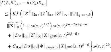
Assume \((Z,Z')\in {\mathscr {D}}^{2\alpha }_X({\mathbb R}^n)\) and \(\Psi \in \mathcal {C}^{q\text {-}var,\tilde{\alpha }}({\mathbb R}^n)\) and \(q, \alpha , \tilde{\alpha }\) satisfy (3.4). For any \(0\le s\le t\le T\), we have the following estimates. The constant K below depends only on \(\Vert \sigma \Vert _{\infty }\), \(\Vert D\sigma \Vert _{\infty }, \Vert D\sigma \Vert _{\gamma -2}, \alpha ,\beta , p,\gamma \) and may change line by line.
-
(1)
$$\begin{aligned} |\Xi _{s,t}|&\le \Bigl \{\Vert \sigma \Vert _{\infty }\Vert X\Vert _{\beta } +\Vert D\sigma \Vert _{\infty }\Vert Z'\Vert _{\infty } \Vert {\mathbb X}\Vert _{2\beta }\omega (s,t)^{\beta }\nonumber \\&\qquad +C_{\beta ,q} \Vert D\sigma \Vert _{\infty } \Vert \Psi \Vert _{q\text {-}var,\tilde{\alpha }} \Vert X\Vert _{\beta }\omega (s,t)^{\tilde{\alpha }}\Bigr \}\omega (s,t)^{\beta }. \end{aligned}$$(3.14)
-
(2)
 (3.15)
and
 (3.16)
where
$$\begin{aligned} f(a,b,c,d)&=a+b+(a^{\gamma -2}+c^{\gamma -2}+d^{\gamma -2})(c+d), \end{aligned}$$(3.17)$$\begin{aligned} g(a,b,c,d)&= f(a,b,c,d)+ c+d. \end{aligned}$$(3.18) -
(3)
 (3.19)
 -
(4)
$$\begin{aligned}&{|\sigma (Y_t)-\sigma (Y_s)|}\nonumber \\&\le \Vert D\sigma \Vert _{\infty } \left\{ \Vert Z'\Vert _{\infty } \Vert X\Vert _{\beta } \omega (s,t)^{\beta -\tilde{\alpha }}+ \Vert R^Z\Vert _{2\alpha }\omega (s,t)^{2\alpha -\tilde{\alpha }} \right. \nonumber \\&\quad \left. +\Vert \Psi \Vert _{q\text {-}var,\tilde{\alpha }}\right\} \omega (s,t)^{\tilde{\alpha }}. \end{aligned}$$(3.20)
-
(5)
\((I(Z,\Psi ),\sigma (Z,\Psi ))\in {\mathscr {D}}^{2\tilde{\alpha }}_X\) holds.


Remark 3.3
(1) Under the condition (3.4), \((\gamma -1)\alpha +\beta >1\) holds as we noted.
(2) If \(\Psi \in \mathcal{C}^{1\text {-}var,\beta }\), then \(I(Z,\Psi )\in {\mathscr {D}}^{2\beta }_X\).
(3) We give estimates of paths on [0, T] in Lemma 3.2. However, a similar estimate holds on small interval \([0,\tau ]\) \((0<\tau <T)\) by replacing the norms and \(\omega (0,T)\) in Lemma 3.2 by the norms on \([0,\tau ]\) and \(\omega (0,\tau )\).
(4) Let \(1/3<\tilde{\beta }<\beta \). Then \(\textbf{X}\) can be regarded as a \(1/\tilde{\beta }\)-rough path. It is easy to check that Lemma 3.2 still holds under the condition (3.4) by replacing \(\beta \) by \(\tilde{\beta }\). Suppose \(\omega (0,T)\le 1\). Then \(\Vert X\Vert _{\tilde{\beta }}\le \Vert X\Vert _{\beta }\) and \(\Vert {\mathbb X}\Vert _{2\tilde{\beta }}\le \Vert {\mathbb X}\Vert _{2\beta }\) holds. We use these results to prove a priori estimate in Theorem 2.7.
Proof
(1) This follows from the explicit form of (3.5) and Lemma 3.1.
(2) This follows from (3.8) and the Sewing lemma.
(3) This follows from (2) and Lemma 3.1.
(4) This follows from the definition of \(Y_t\).
(5) This follows from (3) and (4) and \(2\alpha \ge \tilde{\alpha }\). \(\square \)
We consider the product Banach space \( {\mathscr {D}}^{2\theta _1}_{X}\times \mathcal {C}^{q\text {-}var,\theta _2}, \) where \(1/3<\theta _1\le 1/2\) and \(0<\theta _2\le 1\). The norm is defined by
Let \(\xi \) be the starting point of Z and let \(\eta =A(x)_0\in {\mathbb R}^n\). Note that \(\eta \) is independent of x. Let
The solution of RDE could be obtained as a fixed point of the mapping,
We prove a continuity property of \(\mathcal{M}\).
Lemma 3.4
(Continuity) Assume
where \(\beta _0\) is the number in Assumption 2.2. Then \(\mathcal{M}\) is continuous.
We already proved the compactness of the inclusion \(\mathcal {C}^{q'\text {-}var,\theta '}\subset \mathcal {C}^{q\text {-}var,\theta }\), where \(1\le q'<q,\, q\theta \le q'\theta '\). We need the following compactness result also.
Lemma 3.5
Let \(\frac{1}{3}<\theta <\theta '\le \frac{1}{2}\). Then \({\mathscr {D}}_X^{2\theta '}\subset {\mathscr {D}}^{2\theta }_X\) and the inclusion is compact.
Proof of Lemma 3.5
Suppose
This implies \(\{Z(n)'\}\) is bounded and equicontinuous. Since \(Z(n)_t-Z(n)_s=Z(n)'_sX_{s,t}+R^{Z(n)}_{s,t}\), \(\{Z(n)\}\) is also bounded and equicontinuous. Hence certain subsequence \(\{Z(n_k), Z(n_k)'\}\) converges uniformly. This implies \(\{(Z(n_k)',R^{Z(n_k)})\}\) converges in \({\mathscr {D}}^{2\theta }_X\). \(\square \)
Proof of Lemma 3.4
First note that
\( (\xi +I(Z,\Psi ),\sigma (Y))\in \mathscr {D}^{2\alpha }_X \) follows from Lemma 3.2. By Assumption 2.2, we have
which shows
Thus we have proved (3.26). We estimate \(\Vert I(Z,\Psi )'-I(\tilde{Z},\tilde{\Psi })'\Vert _{\alpha }\). We have
Since \(\beta>\tilde{\alpha }>\alpha \), this shows the continuity of the mapping \(((Z,Z'),\Psi )\mapsto I(Z,\Psi )'\).
We next estimate \(\Vert R^{I(Z,\Psi )}-R^{I(\tilde{Z},\tilde{\Psi })}\Vert _{2\alpha }\).
We argue in a similar way to the sewing lemma for the estimate of the first term. Let \(\mathcal{P}_N=\{t^N_k=s+\frac{k(t-s)}{2^N}\}\) be a usual dyadic partition of [s, t]. We have
By (3.15),

Hence this term is small in the \(\omega \)-Hölder space \(\mathcal {C}^{2\alpha }\) on a bounded set of \(\mathcal {W}_{T,\alpha ,\tilde{\alpha },q,\xi ,\eta }\) if N is large. We fix a partition so that this term is small. Although the partition number may be big,
is a finite sum, and by the explicit form of \(\delta \Xi \) as in (3.6), we see that this difference is small in \(\mathcal {C}^{2\alpha }\) if \(((Z,Z'), \Psi )\) and \(((\tilde{Z},\tilde{Z}'), \tilde{\Psi })\) are sufficiently close in \(\mathcal {W}_{T,\alpha ,\tilde{\alpha },q,\xi ,\eta }\). The estimate of the second and the third terms are similar to the above and we obtain the continuity of the mapping
We next prove the continuity of the mapping
Since we choose \(\beta _0\le \alpha \), it suffices to apply Lemma 2.5 (2) to the case where \(x=\xi +I(Z,\Psi )\) and \(x'=\xi +I(\tilde{Z},\tilde{\Psi })\) because of Lemma 3.2 (2) and the continuity (3.33). \(\square \)
By using the above lemmas, we prove the existence of solutions on small interval \([0,T']\). Since the interval can be chosen independent of the initial condition, we obtain the global existence of solutions and the estimate for solutions. We consider balls with radius 1 centered at \(\left( (\xi +\sigma (\xi ,\eta )X_{t}, \sigma (\xi ,\eta )), \eta \right) \) \((0\le t\le T')\),
Lemma 3.6
(Invariance and compactness) Assume (3.24) and let \(\alpha<\underline{\alpha }<\tilde{\alpha }<\overline{\alpha }<\beta \). Also we choose \(q'>1\) such that \(\displaystyle {\frac{\tilde{\alpha }}{\overline{\alpha }}q<q'<q}\).
-
(1)
For sufficiently small \(T'\), we have
$$\begin{aligned} \mathcal{M}(\mathcal {B}_{T',\alpha ,\tilde{\alpha },q})\subset \mathcal {B}_{T',\underline{\alpha },\overline{\alpha },q'}\subset \mathcal {B}_{T',\alpha ,\tilde{\alpha },q}. \end{aligned}$$(3.36)Moreover \(T'\) does not depend on \(\xi \).
-
(2)
\(\mathcal {B}_{T',\underline{\alpha },\overline{\alpha },q'}\) is a compact subset of \(\mathcal {B}_{T',\alpha ,\tilde{\alpha },q}\).
Proof
(1) The second inclusion is immediate because \(\omega (0,T')\le 1\) and the definition of the norms. We prove the first inclusion. Let \(((Z,Z'),\Psi )\in \mathcal {B}_{T',\alpha ,\tilde{\alpha },q}\). Recall that \(I(Z,\Psi )'_t=\sigma (Z_t,\Psi _t)\) and note that \(\Vert Z'\Vert _{\infty ,[0,T']}\le \Vert \sigma \Vert _{\infty } +\Vert Z'\Vert _{\alpha }\omega (0,T')^{\alpha }\). From Lemma 3.2 (4), we have
We next estimate \(R^{I(Z,\Psi )}\). Let \(0<s<t<T'\). By Lemma 3.2 (3), we have

We turn to the estimate of \(A(\xi +I(Z,\Psi ))\). By (3.27) and Lemma 3.2 (2), we have

Thus, noting Lemma 2.5 (1), there exists a positive number
\(K'\) which depends on K,
\(\Vert \sigma \Vert _{\infty }\),
\(\Vert D\sigma \Vert _{\infty }\), f, g and a positive number
\(\kappa _0\) which depends on
\(\beta -\underline{\alpha }\) and
\(\tilde{\alpha }-\underline{\alpha }\) such that if
 , then
\( \mathcal{M}(\mathcal {B}_{T',\alpha ,\tilde{\alpha },q})\subset \mathcal {B}_{T',\underline{\alpha },\overline{\alpha },q'} \) holds. This completes the proof.
, then
\( \mathcal{M}(\mathcal {B}_{T',\alpha ,\tilde{\alpha },q})\subset \mathcal {B}_{T',\underline{\alpha },\overline{\alpha },q'} \) holds. This completes the proof.
(2) This follows from Lemma 2.1 (2) and Lemma 3.5. \(\square \)
We are in a position to prove our main theorem.
Proof of Theorem 2.7
(1) Let us take
\(\alpha , \tilde{\alpha }, p, q, \underline{\alpha }, \overline{\alpha }\) as in Lemma 3.6. By Lemma 3.4 and Lemma 3.6, applying Schauder’s fixed point theorem, we obtain a fixed point for small interval
\([0,T']\) if
 , where K is a certain positive constant. That is, there exists a solution on
\([0,T']\). We now consider the equation on
\([T',T]\). We can rewrite the equation as
, where K is a certain positive constant. That is, there exists a solution on
\([0,T']\). We now consider the equation on
\([T',T]\). We can rewrite the equation as
Let \(\omega _{T'}(s,t)=\omega (T'+s,T'+t)\) for \(0\le s<t\le T-T'\). We see that \(\tilde{Z}_t:=Z_{T'+t}\) and \(\tilde{\Psi }_{t}:=\Psi _{T'+t}\) \((0\le t\le T-T')\) is a solution to
where
Note that we already defined \( \tilde{A}_{y,T'}(x)_t\) \((0\le t\le T-T')\) \((x\in \mathcal {C}^{\beta }([0,T-T'],{\mathbb R}^n ~|~ x_0=Z_{T'}, \omega _{T'}))\) in Lemma 2.4 (4).
Thanks to Lemma 2.4, we can do the same argument as \([0,T']\) for small interval. By iterating this procedure finite time, say, N-times, we obtain a controlled path \((Z_t,Z_t')\) \((0\le t\le T)\). This is a solution to (2.20). Clearly,

We need to show \((Z,\Psi )\in \mathcal {W}_{T,\beta ,\beta ,1,\xi ,\eta }\) and its estimate with respect to the norm \(\Vert \cdot \Vert _{\beta }\). We give the estimate of the solution on \([0,T']\). The solution \((Z,Z')\) which we obtained satisfies
Let \(0\le u\le v\le T'\). From (3.42), (3.16) and (3.1), we have

Second, by (2.14) and (3.43), we have

Therefore Z and A(Z) are
\((\omega ,\beta )\)-Hölder continuous paths. Hence, we have
 Moreover, we can apply Lemma 3.2 to Z and
\(\Phi =A(Z)\) in the case where
\(\alpha =\tilde{\alpha }=\beta \) and
\(q=1\). Thus, by substituting the estimates (3.43) and (3.44) for (3.19), we obtain for
\(0\le u\le v\le T'\),
Moreover, we can apply Lemma 3.2 to Z and
\(\Phi =A(Z)\) in the case where
\(\alpha =\tilde{\alpha }=\beta \) and
\(q=1\). Thus, by substituting the estimates (3.43) and (3.44) for (3.19), we obtain for
\(0\le u\le v\le T'\),
 These local estimates hold on other small intervals. By the estimate (3.41), we obtain the desired estimate.
(2) Let \((Z,Z')\in \mathscr {D}^{2\beta }_X({\mathbb R}^n)\) be a solution of (2.20). Let \(\beta _0<\tilde{\beta }<\beta \). The constants \(K, \kappa _1,\kappa _2,\kappa _3\) which will appear in the calculation below depend only on \(\sigma \) and F and may change line by line. As we already noted in Remark 3.3 (4), Lemma 3.2 still holds replacing \(\beta \) by \(\tilde{\beta }\). We take \(0<\tau \le T\) so that \(\omega (0,\tau )\le 1\). Using \(\Vert X\Vert _{\tilde{\beta },[0,\tau ]}\le \Vert X\Vert _{\beta ,[0,\tau ]}\) and \(\Vert {\mathbb X}\Vert _{\tilde{\beta },[0,\tau ]}\le \Vert {\mathbb X}\Vert _{\beta ,[0,\tau ]}\) which follows from \(\omega (0,\tau )\le 1\), we have
By Lemma 2.5 (1), we have
which implies
By (3.45) and (3.47), we obtain
We apply Lemma 3.2 (3) to the estimate of \(R^Z\) in the case where \(\Psi =A(Z)\), \(q=1\) and \(\alpha =\tilde{\alpha }=\tilde{\beta }\). By combining the estimates obtained above, we see that there exist \(\kappa _1>0, \kappa _2>1,\kappa _3>0\) and \(K>0\) which can be taken independent of \(\tilde{\beta }\) such that

Let \( z_{\tilde{\beta },\tau }=\Vert Z'\Vert _{\tilde{\beta },[0,\tau ]}+\Vert R^Z\Vert _{2\tilde{\beta },[0,\tau ]}. \) Then using (3.48) and (3.49), we see that there exist (possibly different) \(\kappa _1\ge 1, \kappa _2>1, \kappa _3>0, K>0\) which can be taken independent of \(\tilde{\beta }\) such that

Since \(\tilde{\beta }<\beta \), the function \(\tau \mapsto z_{\tilde{\beta },\tau }\) \((0\le \tau \le 1)\) is an increasing continuous function and \(\lim _{\tau \rightarrow +0}z_{\tilde{\beta }, \tau }=0\). If  , then by the definition, \(Z_t=\xi \) for all \(0\le t\le T\) and \(\Vert Z'\Vert _{\beta }=\Vert R^Z\Vert _{2\beta }=0\) hold. The desired estimate holds. So we assume
  . We now define

There are two cases \(\tau _{1}=T\) and \(\tau _{1}<T\). Suppose \(\tau _{1}=T\). Then  holds. If this is not the case,
  holds. Hence by the inequality (3.50), we get

After establishing this estimate, we proceed in a similar way to the argument in the proof of (1) replacing \(T'\) by \(\tau _1\). In this way, we obtain an increasing time sequence \( 0=\tau _0<\tau _1<\cdots<\tau _{N-1}<\tau _N=T \) \((N\ge 2)\) and the estimate (3.51) hold for \(\omega (\tau _{i-1},\tau _i)\) \((1\le i\le N-1)\). Also we have


By using \(\sum _{i=1}^{N-1}\omega (\tau _{i-1},\tau _i)\le \omega (0,T)\), we get the estimate of N as follows.

Using (3.52), (3.53), (3.54) and simple estimates
we obtain

Since \(\tilde{\beta }<\beta \) and \(\Vert Z'\Vert _{\beta , [0,T]}+\Vert R^Z\Vert _{2\beta , [0,T]}<\infty \), taking the limit \(\tilde{\beta }\uparrow \beta \), this estimate hold for the norms \(\Vert \cdot \Vert _{\beta }\) and \(\Vert \cdot \Vert _{2\beta }\) as well. The estimates of Z and A(Z) follow from this estimate and the estimates similar to (3.45) and (3.47). This completes the proof. \(\square \)
4 A Continuity Property of the Solution Mapping
In this section, we consider the case where \(\omega (s,t)=|t-s|\). That is, we consider usual Hölder rough paths. Also let us denote the set of \(\beta \)-Hölder geometric rough paths (\(1/3<\beta \le 1/2\)) by \(\mathscr {C}^{\beta }_g({\mathbb R}^d)\) which is the closure of the set of smooth rough paths in the topology of \(\mathscr {C}^{\beta }({\mathbb R}^d)\). In this paper, smooth rough path means the rough path \(\textbf{h}\) defined by a Lipschitz path \(h\in \mathcal {C}^1\) and its iterated integral \(\bar{h}^2_{s,t}= \int _s^t(h_u-h_s)\otimes dh_u\). We identify \(\textbf{h}\) and the Lipschitz path h. Also we denote the set of smooth rough paths by \(\mathscr {C}_{\textrm{Lip}}({\mathbb R}^d)\).
Let \(Z(\textbf{h})\) be a solution to (2.20) for \(\textbf{X}=\textbf{h}\). Then \(Z(\textbf{h})\) is a solution to the usual integral equation
As already explained, we cannot expect the uniqueness of the solution of the RDEs in our setting driven by general rough path \(\textbf{X}\). However, the uniqueness hold in many cases when the driving rough path is a smooth rough path and \(\sigma \) is sufficiently smooth. If the solution to the ODE (4.1) is unique, then \(Z(\textbf{h})\) is uniquely defined and \((Z(\textbf{h}),R^{Z(\textbf{h})},A(Z(\textbf{h})))\) satisfies the same estimate as in Theorem 2.7. We use the notation \(Z(h)_t\) instead of \(Z(\textbf{h})_t\) in this case.
We denote the set of solutions \((Z,Z')\) of our RDE (2.20) by \(Sol(\textbf{X})\). We prove a certain continuity property of multivalued mapping \(\textbf{X}\mapsto Z(\textbf{X})\in Sol(\textbf{X})\) at the rough path \(\textbf{X}\) for which the solution is unique. Thus, this multivalued map is continuous in such a sense at any smooth rough path if the uniqueness holds on the set of smooth rough paths.
We write \(\mathcal {C}^{\theta -}=\cap _{0<\varepsilon<\theta }\mathcal {C}^{\theta -\varepsilon }, \mathcal {C}^{1+\text {-}var,\theta -}=\cap _{q>1,0<\varepsilon <\theta }\mathcal {C}^{q\text {-}var,\theta -\varepsilon }\). Clearly, these spaces are Fréchet spaces with the naturally defined semi-norms. Also note that \(Z(\textbf{X})\in \mathcal {C}^{\beta -}([0,T],{\mathbb R}^n)\).
Lemma 4.1
We consider the Eq. (2.20) and assume the same assumption on A and \(\sigma \) in Theorem 2.7. Let \(\textbf{X}\in \mathscr {C}^{\beta }({\mathbb R}^d)\). Let \(\{\textbf{X}_N\}\subset \mathscr {C}^{\beta }({\mathbb R}^d) \) be a sequence such that  . Let us choose solutions \(Z(\textbf{X}_N)\in Sol(\textbf{X}_N)\) \((N=1,2,\ldots )\). Then there exists a subsequence \(N_k\uparrow \infty \) such that the limit \(Z=\lim _{k\rightarrow \infty }Z(\textbf{X}_{N_k})\) exits in \(\mathcal {C}^{\beta -}([0,T], {\mathbb R}^n)\). Further for such Z, \((Z,\sigma (Z,A(Z)))\in Sol(\textbf{X})\) and \( \lim _{k\rightarrow \infty }\left\| R^{Z(\textbf{X}_{N_k})}-R^{Z}\right\| _{2\beta -} =0 \) hold.
Proof
By the estimate in Theorem 2.7 (2), we can choose \(\{N_k\}\) such that \(Z(\textbf{X}_{N_k}), \) \( A(Z(\textbf{X}_{N_k}))\) converges in \(\mathcal {C}^{\beta -}\) and \(\mathcal {C}^{1+\text {-}var, \beta -}\) respectively. This implies \(\lim _{k\rightarrow \infty }\int _s^tA(Z(\textbf{X}_{N_k}))_{s,r} dX_{N_k}(r) =\int _s^tA(Z(\textbf{X}))_{s,r}dX_r\) which shows the limit Z satisfies the inequality (2.22).
This proves \((Z,\sigma (Z,A(Z)))\in Sol(\textbf{X})\). We have
Hence \(\lim _{k\rightarrow \infty }R^{Z(\textbf{X}_{N_k})}_{s,t}=R^{Z(\textbf{X})}_{s,t}\) for all (s, t). Combining the uniform estimates of \((\omega ,2\beta )\)-Hölder estimates of them, this completes the proof. \(\square \)
The following proposition follows from the above lemma
Proposition 4.2
We consider the Eq. (2.20) and assume the same assumption on A and \(\sigma \) in Theorem 2.7. Assume the solution of (2.20) is unique for the rough path \(\textbf{X}_0\in \mathscr {C}^{\beta }({\mathbb R}^d)\). Then the multivalued mapping \(\textbf{X} (\in {\mathscr {C}}^{\beta }({\mathbb R}^d))\rightarrow Sol(\textbf{X})\) is continuous at \(\textbf{X}_0\) in the following sense. For any \(\varepsilon >0\), there exists \(\delta >0\) such that for any \(\textbf{X}\) satisfying  and any \(Z(\textbf{X})\in Sol(\textbf{X})\), it holds that
Remark 4.3
Let \(\textbf{X}\in \mathscr {C}^{\beta }_g({\mathbb R}^d)\). It holds that for any sequence \(\{\textbf{h}_N\}\subset \mathscr {C}_{\textrm{Lip}}({\mathbb R}^d)\) satisfying  , any accumulation points of \(\{Z(h_{N})\}\) belong to \(Sol(\textbf{X})\). The set \(Sol_{\infty }(\textbf{X})\) which consists of such all accumulation points is a subset of \(Sol(\textbf{X})\) and may be a natural class of solutions. However \(Sol_{\infty }(\textbf{X})=Sol(\textbf{X})\) may hold.
By a similar argument to the proof of Theorem 4.9 in [2], we can prove the existence of universally measurable selection mapping of solutions as follows.
Proposition 4.4
We consider the Eqs. (3.1) and (3.2) and assume the same assumption on A and \(\sigma \) in Theorem 2.7. Then there exists a universally measurable mapping
which satisfies the following.
-
(1)
\(\left( Z(\textbf{X}),\sigma (Y(\textbf{X}))\right) \in {\mathscr {D}}^{2\beta }_X({\mathbb R}^n)\) and \(\Bigl ( \left( Z(\textbf{X}),\sigma (Y(\textbf{X}))\right) , \Psi (\textbf{X}) \Bigr )\) is a solution in Theorem 2.7 and satisfies the estimate in (5.13).
-
(2)
There exists a sequence of Lipschitz paths \(h_N\) such that
 and \(\mathcal{I}(\textbf{h}_N)\) converges to \(\mathcal{I}(\textbf{X})\) in \(\mathcal {C}^{\beta -}({\mathbb R}^n)\times \mathcal {C}^{\beta -}(\mathcal{L}({\mathbb R}^d,{\mathbb R}^n))\times \mathcal {C}^{1\text {-}var+,\beta -}({\mathbb R}^d)\).
 and
and Proof
Below, we omit writing \(\xi \). We consider the product space,
and its subset
Let \(\bar{E}_0\) be the closure of \(E_0\) in E. Then \(\bar{E}_0\) is a separable closed subset of E. The separability follows from the continuity of the mapping \(h\mapsto \left( (Z(h), \sigma (Y(h))), \Psi (h)\right) \). Note that \(Sol_{\infty }(\textbf{X})\) coincides with the projection of the subset of \(\bar{E}_0\) whose first component is \(\textbf{X}\). Hence by the measurable selection theorem (See 13.2.7. Theorem in [15]), there exists a universally measurable mapping \(\mathcal{I}: {\mathscr {C}}^{\beta }_g({\mathbb R}^d)\rightarrow E \) such that \(\mathcal{I}(\textbf{X})\in \left\{ \textbf{X}\right\} \times Sol_{\infty }(\textbf{X})\). This mapping satisfies the required properties in (1) and (2). \(\square \)
Remark 4.5
It is not clear that we could obtain the adapted measurable solution mapping \(\mathcal {I}\).
5 Examples
5.1 Reflected Rough Differential Equations
Let D be a connected domain in \({\mathbb R}^n\). As in [27, 34], we consider the following conditions (A), (B) on the boundary. See also [35].
Definition 5.1
We write \(B(z,r)=\{y\in {\mathbb R}^n\,|\, |y-z|<r\}\), where \(z\in {\mathbb R}^n\), \(r>0\). The set \(\mathcal{N}_x\) of inward unit normal vectors at the boundary point \(x\in \partial D\) is defined by
-
(A)
There exists a constant \(r_0>0\) such that
$$\begin{aligned} \mathcal{N}_x=\mathcal{N}_{x,r_0}\ne \emptyset \quad \text{ for } \text{ any }~x\in \partial D. \end{aligned}$$ -
(B)
There exist constants \(\delta >0\) and \(0<\delta '\le 1\) satisfying: for any \(x\in \partial D\) there exists a unit vector \(l_x\) such that
$$\begin{aligned} (l_x,{\varvec{n}})\ge \delta ' \qquad \text{ for } \text{ any }~{\varvec{n}}\in \cup _{y\in B(x,\delta )\cap \partial D}\mathcal{N}_y. \end{aligned}$$
Let us recall the Skorohod equation. The Skorohod equation associated with a continuous path \(x\in C([0,\infty ), {\mathbb R}^n)\) with \(x_0\in \bar{D}\) is given by
Under the assumptions (A) and (B) on D, the Skorohod equation is uniquely solved. This is due to Saisho [34]. We write \(\Gamma (x)_t=y_t\) and \(L(x)_t=\phi _t\). By the uniqueness, we have the following flow property.
Lemma 5.2
Assume (A) and (B). For any continuous path x on \({\mathbb R}^n\) with \(x_0\in {\bar{D}}\), we have for all \(\tau , s\ge 0\)
where \((\theta _sx)_{\tau }=x_{\tau +s}-x_s\).
We obtain the following estimate of L(x).
Lemma 5.3
Assume conditions (A) and (B) hold. Let \(x_t\) be a continuous path of finite q-variation \((q\ge 1)\). Then we have the following estimate.
where C is a positive constant which depends on the constants \(\delta , \delta ', r_0\) in conditions (A) and (B).
Proof
We proved the following estimate in [2, 4] following the argument in [34].
where
By combining this and Lemma 2.5, we complete the proof. \(\square \)
Lemma 5.4
Assume (A) and (B). Consider two Skorohod equations \(y=x+\phi \), \(y'=x'+\phi '\). Then
The estimate (5.10) can be found in Remark 4.1 (i) in [34]. Lemma 5.3 shows that if x is a \((\omega ,\theta )\)-Hölder continuous path, \(L(x)\in \mathcal {C}^{1\text {-}var,\theta }\) holds true. Actually, \(\Vert L(x)\Vert _{1\text {-}var, [s,t]}\) can be estimated by the modulus of continuity of x and \(\Vert x\Vert _{\infty \text {-}var,[s,t]}\). For example, see [34] and the proof of Lemma 2.3 in [4]. Hence, we see that L is a 1/2-Hölder continuous map on \(C([0,\infty ), {\mathbb R}^n)\). Note that \(\Gamma \) is Lipschitz continuous if D is a convex polyhedron ([16]).
Let \(\textbf{X}\in \mathscr {C}^{\beta }({\mathbb R}^d)\). We assume D satisfies the condition (A) and (B). We now consider reflected RDE:
We need to make clear the definition of the solution \((Y_t)\) of (5.11).
Definition 5.5
We call \(Y_t\) is a solution of (5.11) if and only if the following holds:
-
(i)
There exist a \(Z\in \mathscr {D}^{2\beta }([0,T],{\mathbb R}^n)\) and a continuous bounded variation path \(\Phi _t\) such that \(Y_t=Z_t+\Phi _t\) \((0\le t\le T)\).
-
(ii)
\(\Phi _t=L(Z)_t\) \((0\le t\le T)\).
-
(iii)
Z satisfies
$$\begin{aligned} Z_t&=\xi +\int _0^t\sigma (Z_s+L(Z)_s)d\textbf{X}_s,\quad Z_t'=\sigma (Z_t+L(Z)_t) \qquad 0\le t\le T. \end{aligned}$$(5.12)
Note that if Y is a solution in the above sense, Z is uniquely determined by Y and \(\textbf{X}\) since \(Z_t=\xi +\int _0^t\sigma (Y_s)d\textbf{X}_s\) and \(Z'_t=\sigma (Y_t)\) hold. See also Remark 5.7 (1).
By applying Theorem 2.7, we obtain the following result.
Theorem 5.6
Let \(\textbf{X}\in \mathscr {C}^{\beta }({\mathbb R}^d)\). Assume D satisfies conditions (A) and (B).
Let \(\sigma \in \textrm{Lip}^{\gamma -1}({\mathbb R}^n, \mathcal{L}({\mathbb R}^d,{\mathbb R}^n))\) and \(\xi \in \bar{D}\). Then there exist \((Z,Z')\in {\mathscr {D}}^{2\beta }_X({\mathbb R}^n)\) and \(\Phi \in \mathcal {C}^{1\text {-}var,\beta }({\mathbb R}^n)\) with \(\Phi _0=0\) such that \(Y_t=Z_t+\Phi _t\) is a solution of (5.11). Moreover the following estimate holds,

where \(K, \kappa _i\) are constants which depend only on \(\sigma ,\beta ,\gamma , \delta , \delta ', r_0\).
Proof
By applying Theorem 2.7, we have at least one solution Z and the estimate of (5.12). Let \(Y_t=Z_t+L(Z)_t\) and \(\Phi _t=L(Z)_t\). Then this pair is a solution to the original equation. \(\square \)
Remark 5.7
(1) Let \((Y_t,\Phi _t)\) be a solution of (5.11). Then there exists \(\theta >1\) such that
Conversely, suppose
-
(i)
\((Y_t,\Phi _t)\) is a pair of continuous paths satisfying (5.14) and \((\Phi _t)\) is a bounded variation path satisfying \(\Vert \Phi \Vert _{1\text {-}var,[s,t]}\le C\omega (s,t)^{\beta }\) \((0\le s\le t\le T)\).
-
(ii)
\(Y_t\in \bar{D}\) \((0\le t\le T)\).
-
(iii)
\((Y_t,\Phi _t)\) satisfies
$$\begin{aligned} \Phi _t=\int _0^t1_{\partial D}(Y_s){\varvec{n}}(s)d\Vert \Phi \Vert _{1\text {-}var,[0,s]} \quad \quad 0\le t\le T,\quad ({\varvec{n}}(s)\in \mathcal {N}_{Y_s}\quad \text {if }Y_s\in \partial D). \end{aligned}$$
Let \(\Xi _{s,t}=\sigma (Y_s)X_{s,t}+(D\sigma )(Y_s)[\sigma (Y_s)]\mathbb {X}_{s,t}+ (D\sigma )(Y_s)\left( \int _s^t\Phi _{s,u}\otimes dX_u\right) \). Then \(|(\delta \Xi )_{s,u,t}|\le C\omega (s,t)^\theta \) \((0\le s\le u\le t\le T)\) holds and \(Z_{0,t}\in \mathcal {C}^{\beta }([0,T],{\mathbb R}^n; x_0=0)\) exists such that \(|(Z_{0,t}-Z_{0,s})-\Xi _{s,t}|\le C\omega (s,t)^\theta \). Further, by the assumption on \(\Phi \), \((Z_{0,t})\in \mathscr {D}^{2\beta }_X({\mathbb R}^n)\) with \(Z_{0,t}'=\sigma (Y_t)\) and \(Y_t=Y_0+Z_{0,t}+\Phi _t\) holds. Clearly, \(Z_{0,t}=\int _0^t\sigma (Y_s)d\textbf{X}_s\). By the definition of L, we have \(L(Y_0+Z_{0,\cdot })_t=\Phi _t\). Hence, \((Y_t,\Phi _t)\) is a solution of (5.11).
(2) In [2], we consider the following condition (H1) on D:
-
(i)
The condition (A) holds,
-
(ii)
There exists a positive constant C such that for any x, it holds that
$$\begin{aligned} \Vert L(x)\Vert _{1\text {-}var, [s,t]}&\le C\Vert x\Vert _{\infty \text {-}var,[s,t]}. \end{aligned}$$
This condition holds if D is convex and there exists a unit vector \(l\in {\mathbb R}^n\) such that
Under (H1) and \(\sigma \in C^3_b\), we proved the existence of solutions of reflected RDEs driven by \(1/\beta \) rough paths and gave estimates for the solutions in Theorem 4.5 in [2]. We used Euler approximation of the solution modifying Davie’s proof in [9]. In the proof, we need to solve the following implicit Skorohod equation in each step,
where \(0<T'<T\), \(y_t\in \bar{D}\) \((0\le t\le T')\), \(M\in \mathcal {L}({\mathbb R}^n\otimes {\mathbb R}^d,{\mathbb R}^n)\) and \(\Phi _t\) is a continuous bounded variation path. Also \(\eta _t\), \(x_t\) are finite \(1/\beta \)-variation paths which are defined by X and \({\mathbb X}\). If we replace \(\int _0^t\Phi _r\otimes dx_r\) in (5.15) and (5.16) by \(\int _0^tf(\Phi _r)\otimes dx_r\), where f is a bounded Lipschitz map between \({\mathbb R}^n\), then we can solve the equation under general condition (A) and (B). To avoid the explosion problem, that is, to handle the linear growth term of \(\Phi _t\), we put stronger assumption (H1)(ii) on D in [2]. Also we used Lyon’s continuity theorem of rough integrals in the proof and so we need to assume \(\sigma \in C^3_b\). In this paper, we adopt different approach to the problem and obtain an extension of the previous result in the sense that the assumption on \(\sigma \) and D can be relaxed.
In Sect. 4, we prove a continuity property of solution mappings at Lipschitz paths under the uniqueness of the solutions. For reflected RDEs, we can give more explicit estimate of the continuity of the solution mapping Y at the Lipschitz paths. As before we consider a domain \(D\subset {\mathbb R}^n\) which satisfies the conditions (A) and (B). Let h be a Lipschitz path on \({\mathbb R}^d\) starting at 0. If \(\sigma \) is Lipschitz continuous, there exists a unique solution \((Y(h,\xi )_t,\Phi (h,\xi )_t)\) to the reflected ODE in usual sense (see Proposition 4.1 in [4] for example),
We may omit denoting \(h,\xi \). Moreover, \(Z(h)_t=\xi +\int _0^t\sigma (Y_s(h))dh_s\), \(Z_t(h)'=\sigma (Y_t(h))\) and \(\Phi (h)_t\) are a unique pair of solution to the equation in Theorem 5.6 for the smooth rough path \(\textbf{h}_{s,t}=(h_{s,t},\bar{h}^2_{s,t})\) defined by h. Hence the solution \((Z(h),R^{Z(h)},\Phi (h))\) satisfies the estimate (5.13) with the same constant \(C_1, C_2\).
From now on, we will give an explicit estimate for \(Y_t(\xi ,\textbf{X})-Y_t(\eta ,h)\). Let \(\textbf{X}\) be a general (not necessarily geometric) \(\beta \)-Hölder rough path. Let \(\textbf{X}^{-h}_{s,t}\) be the translated rough path of \(\textbf{X}\) by h. That is, the 1st level path and the second level path are given by,
Hence
These imply that if  , then

By the definition of controlled paths, we immediately obtain the following.
Lemma 5.8
Let \(\textbf{X}\in \mathscr {C}^{\beta }_g({\mathbb R}^d)\). Let h be a Lipschitz path. If \((Z,Z')\in \mathscr {D}_X^{2\beta }\), then \((Z,Z')\in \mathscr {D}_{X-h}^{2\beta }\). In fact,
Let \((Z,Z')\in {\mathscr {D}}^{2\alpha }_X({\mathbb R}^n)\) and \(\Phi \in \mathcal {C}^{q\text {-}var,\tilde{\alpha }}({\mathbb R}^n)\) with \(\Phi _0=0\) and \(q, \alpha , \tilde{\alpha }\) satisfy the assumptions in Lemma 3.1. By the above lemma, we can define the integral \(\int _s^t\sigma (Y_u)d\textbf{X}^{-h}_u\) and the estimates in Lemma 3.2 hold for this integral. Here \(Y_u=Z_u+\Phi _u\). Moreover, \(\Xi _{s,t}\) in (3.5) which is defined by \(\textbf{X}^{-h}_{s,t}\) reads
where
Since \(|\tilde{\Xi }_{s,t}|\le C(t-s)^{1+\tilde{\alpha }}\), the sum of these terms converges to 0. Thus we obtain
We now consider the following condition on the boundary.
Definition 5.9
(Condition (C)) There exists a \(Lip^{\gamma }\) function f on \({\mathbb R}^n\) and a positive constant k such that for any \(x\in \partial D\), \(y\in \bar{D}\), \({\textbf{n}}\in \mathcal{N}_x\) it holds that
Usually, the function f is assume to be \(C^2_b\) in the condition (C). See [27, 34]. Here, we assume \(f\in Lip^{\gamma }\) to make use of estimates in Lemma 3.2.
Under additional condition (C), we can prove the following explicit modulus of continuity.
Lemma 5.10
Let \(\textbf{X}\in \mathscr {C}^{\beta }_g({\mathbb R}^d)\). Assume that D satisfies the conditions (A), (B), (C) and \(\sigma \in \textrm{Lip}^{\gamma -1}\). Let \(Y_t(\textbf{X},\xi ), Z_t(\textbf{X},\xi ), \Phi _t(\textbf{X},\xi ), Y_t(h,\zeta ), \Phi _t(h,\zeta )\) be a solution as in Lemma 4.1. Assume  . Then there exists a positive constant C which depends only on \(\sigma , r_0, \delta , \delta ', f, k\) such that

Proof
We write \(Y_t=Y_t(\textbf{X},\xi )\), \(\Phi (\textbf{X},\xi )_t=\Phi _t\) and \(\tilde{Y}_t=Y(h,\zeta )_t\), \(\tilde{\Phi }_t=\Phi (h,\zeta )_t\) for simplicity. Let \( Z_t=e^{-\frac{2}{k}\left( f(Y_t)+f(\tilde{Y}_t)\right) } |Y_t-\tilde{Y}_t|^2. \) We have
Condition (C) implies that the fourth integral on the right-hand side of the Eq. (5.30) is always negative. By the estimates of the solution \(Y, \tilde{Y}, \Phi , \tilde{\Phi }\) in Theorem 5.6 and the estimates in Lemma 3.2 and the Gronwall inequality, we obtain the desired estimate. \(\square \)
5.2 Perturbed Reflected SDEs: A Short Review
Let us recall basic results for the following equation driven by a continuous path \(x_t\) on \({\mathbb R}\),
When \(x_t\) is a sample path of a standard Brownian motion, the solutions to (5.31) and (5.32) are called (doubly) perturbed Brownian motion and perturbed reflected Brownian motion respectively.
First we consider the Eq. (5.31). Clearly, if either \(a\ge 1\) or \(b\ge 1\), then there are no solutions to this equation for certain x. So we consider the case where \(a<1\) and \(b<1\). Suppose \(b=0\). Then we have explicitly, \(Y_t=x_t+\frac{a}{1-a}\sup _{0\le s\le t}x_s\). By [7], when \(|\frac{ab}{(1-a)(1-b)}|<1\), a fixed point argument works and the unique existence holds for any continuous path \(x_t\) with \(x_0=0\). The unique existence extends to \(|\frac{ab}{(1-a)(1-b)}|=1\) by [10]. Consider the case where \(x_t\) is a sample path of 1-dimensional Brownian motion \(W_t\) with \(W_0=0\). For any \(0\le a<1\), \(0\le b<1\), it is proved in [31] that the pathwise uniqueness holds and the solution is adapted to the Brownian filtration. Finally, for any \(a<1, b<1\), the same results is proved in [8].
We consider the Eq. (5.32). By a fixed point argument, the unique existence is proved in [25] the case (1) \(a<1/2\) and (2) \(a<1\) with \(x_0>0\). Next, the pathwise uniqueness is proved by [8] for \(a<1\) when \(x_t\) is the Brownian path \(W_t\) with \(W_0=0\). The unique existence for \(a<1\) is extended by [13] for any continuous path \(x_t\).
We next explain results for the variable coefficient version driven by a standard 1-dimensional Brownian motion \(W_t\),
where \(\sigma \) is a Lipschitz continuous function on \({\mathbb R}\) and the integral is the Itô integral. The unique existence of the solution to (5.33) is proved for \(a<1\) by [13]. The same authors prove the unique existence of the solution to (5.34) for two cases where (1) \(a<1\) and \(\xi >0\) and (2) \(0\le a<1/2\) and \(\xi =0\). Under the same assumption on a, the absolutely continuity of the law of \(Y_t\) with respect to the Lebesgue measure was studied in [36].
5.3 Perturbed Reflected Rough Differential Equations
We consider the multidimensional versions of (5.33) and (5.34) driven by rough paths. Our objectives are the following two equations.
where \(e_n={}^t(0,\ldots ,0,1)\) and \(\sigma \in \textrm{Lip}^{\gamma -1}({\mathbb R}^n,\mathcal {L}({\mathbb R}^d,{\mathbb R}^n))\). We assume that C is a mapping from \(C([0,T],{\mathbb R}^n)\) to the subspace of continuous and bounded variation paths on \({\mathbb R}^n\) and \(\{C(x)_s\}_{0\le s\le t}\) is measurable with respect to \(\sigma (\{x_s\}_{0\le s\le t})\) for all \(0\le t\le T\). The first Eq. (5.35) is a perturbed rough differential equations and the second Eq. (5.36) is a perturbed reflected rough differential equation on \(\bar{D}=\{(x_1,\ldots ,x_n)~|~x_n\ge 0\}\). \(\Phi _te_n\) is the reflected term and \(Y_t\) and \(\Phi _t\) should satisfy
In both equations, \(Y_0\ne \xi \) in general. Consider the case \(t=0\). Then we have \( Y_0=\xi +C(Y)_0. \) Since C(Y) is adapted, \(C(Y)_0\) is a function of \(Y_0\) and we may write \(C(Y)_0=C_0(Y_0)\). Hence \(Y_0\) should satisfy \(Y_0=\xi +C_0(Y_0)\) and we need to assume \(Y_0\in \bar{D}\). If we consider the case where \(Y_t\in {\mathbb R}\) and \(C(Y)_t=a\max _{0\le s\le t}Y_s\) \((a<1)\), \(Y_0=\frac{1}{1-a}\xi \) holds. In this case, \(Y_0\ge 0\) and \(\xi \ge 0\) are equivalent and so \(Y_t\) starts from \([0,\infty )\) when \(\xi \ge 0\). Under the assumption that \(Y_0=\xi +C_0(Y_0)\in \bar{D}\), by the explicit solution of the Skorohod problem, we have
where \(a\vee b=\max (a,b)\).
We give the definition of the solution of (5.35) and (5.36).
Definition 5.11
(1) \(Y_t\) is a solution of (5.35) if the following hold.
-
(i)
There exists a \(Z\in \mathscr {D}^{2\beta }_X({\mathbb R}^n)\) such that \(Y_t=Z_t+C(Y)_t\) and \(Z'_t=\sigma (Y_t)\) \((0\le t\le T)\) hold.
-
(ii)
\(Z_t=\xi +\int _0^t\sigma (Z_s+C(Y)_s)d\textbf{X}_s\) \((0\le t\le T)\) holds.
(2) \((Y_t,\Phi _t)\) is a solution of (5.36) if the following holds:
- (i)
-
(ii)
There exists a \(Z\in \mathscr {D}^{2\beta }_X({\mathbb R}^n)\) such that \(Y_t=Z_t+C(Y)_t+\Phi _te_n\) and \(Z'_t=\sigma (Y_t)\) \((0\le t\le T)\) hold.
-
(iii)
\(Z_t=\xi +\int _0^t\sigma (Z_s+C(Y)_s+\Phi _se_n)d\textbf{X}_s\) \((0\le t\le T)\) holds.
We solve these equations by transforming them to the equations in Theorem 2.7. To this end, we introduce the following conditions.
Definition 5.12
For a mapping \(C: C([0,T], {\mathbb R}^n)\rightarrow C([0,T], {\mathbb R}^m)\), we consider the following conditions, where \(\rho \) denotes a positive number.
- \(\mathrm{(Lip)}_{\rho }\):
-
\(\Vert C(x)-C(y)\Vert _{\infty ,[0,t]}\le \rho \Vert x-y\Vert _{\infty ,[0,t]}\) for all \(x,y\in C([0,T], {\mathbb R}^n)\) and \(0\le t\le T\).
- \(\mathrm{(BV)}_{\rho }\):
-
\(\Vert C(x)\Vert _{1\text {-}var, [s,t]}\le \rho \Vert x\Vert _{\infty \text {-}var, [s,t]}\) for all \(0\le s\le t\le T\).
We may write \(C\in (\textrm{Lip})_{\rho }\) simply when C satisfies the condition \((\textrm{Lip})_{\rho }\), etc. Also we denote by \(\Vert C\Vert _{\textrm{Lip}}\) the smallest nonnegative number \(\rho \) for which \((\textrm{Lip})_{\rho }\) holds.
Clearly the conditions \(\mathrm{(Lip)}_{\rho }\) and \(\mathrm{(BV)}_{\rho }\) are stronger than the conditions in Assumption 2.2. Also the conditions \(\mathrm{(Lip)}_{\rho }\) and \(\mathrm{(BV)}_{\rho }\) imply the conditions (A1), (A2) and (A3) in [1].
As we noted, C which is defined in Example 2.9 (2) satisfies the above conditions.
Proposition 5.13
Let \(\rho >0\). Let \(f: {\mathbb R}^n\rightarrow {\mathbb R}\) be a Lipschitz function satisfying \((\textrm{Lip})_{\rho }\). Let \(C(x)_t=\max _{0\le s\le t}f(x_s)\) for \(x\in C([0,T],{\mathbb R}^n)\). Then we have \(C\in \mathrm{(Lip)}_{\rho }\cap \mathrm{(BV)}_{\rho }\).
Proof
We consider the simplest case \(C(x)_t=\max _{0\le s\le t}x_s\), where x is a continuous path on \({\mathbb R}\). Let \(0\le s<t\). We take values \(0\le s_{*}\le s, 0\le t_{*}\le t\) such that \(C(x)_{s}=x_{s_{*}}\) and \(C(x)_{t}=x_{t_{*}}\). Suppose \(t_{*}\le s\), then \(C(x)_u=C(x)_{t_{*}}\) \((s\le u\le t)\) holds. Hence \(\Vert C(x)\Vert _{1\text {-}var, [s,t]}=0\). Suppose \(s<t_{*}\le t\). Then using \(x_s\le x_{s_{*}}\), we have
which implies the validity of \((\textrm{BV})_1\). We next show \((\textrm{Lip})_1\). Let \(x, x'\) be continuous paths on \({\mathbb R}\). Similarly, \(t'_{*}\) denotes a time at which \(x'\) attains its maximum of \(x_u\) \((0\le u\le t)\). We have \(C(x)_t-C(x')_t=x_{t_{*}}-x'_{t'_{*}}\). If \(x_{t_{*}}-x'_{t'_{*}}=0\), Suppose \(x_{t_{*}}>x'_{t'_{*}}\). Then, by \(x'_{t'_{*}}\ge x'_{t_{*}}\), we have
This proves that \((\textrm{Lip})_{1}\) holds for \(C(x)_t=\max _{0\le s\le t}x_s\). General cases follow from this simplest case. \(\square \)
We consider (5.35). To this end, we consider the following condition on C.
\((\textbf{Condition}~ \tilde{\textbf{C}})\) (i) For any \(x\in C([0,T],{\mathbb R}^n)\), there exists unique \(y\in C([0,T],{\mathbb R}^n)\) such that \(y=x+C(y)\). Define \(\tilde{C}(x)=y-x\).
(ii) \(\tilde{C}\) satisfies \(\mathrm{(Lip)}_{\rho '}\) for certain \(\rho '\).
About this property, we have the following. The proof is straightforward and so we omit the proof.
Proposition 5.14
Assume C satisfies \((\textrm{Condition}~ \tilde{\textrm{C}})\) \(\mathrm{(i)}\). Then for any \(0\le t\le T\) and \(x\in C([0,t],{\mathbb R}^n)\), there exists a unique \(y\in C([0,t],{\mathbb R}^n)\) such that \(y=x+C(y)\) on [0, t]. For these x and y, we define \(\tilde{C}_t(x)=y-x\in C([0,t],{\mathbb R}^n)\). Then for any \(z\in C([0,T],{\mathbb R}^n)\) satisfying \(z_s=x_s\) \((0\le s\le t)\), \(\tilde{C}(z)_s=\tilde{C}_t(x)_s\) \((0\le s\le t)\) holds.
By this result, given \(\xi \in {\mathbb R}^n\), the solution \(\eta \in {\mathbb R}^n\) of \(\eta =\xi +C_0(\eta )\) is unique if C satisfies \((\textrm{Condition}~ \tilde{\textrm{C}})\) \(\mathrm{(i)}\). We have the following result for (5.35).
Theorem 5.15
Let C be a continuous mapping between \(C([0,T], {\mathbb R}^n)\). Suppose C satisfies \((\textrm{Condition}~ \tilde{\textrm{C}})\) and \(\tilde{C}\) satisfies \((\textrm{BV})_{\rho ''}\) for certain \(\rho ''\). Let \(\textbf{X}\in \mathscr {C}^{\beta }({\mathbb R}^d)\).
-
(1)
There exists a controlled path \(Z\in {\mathscr {D}}^{2\beta }_X({\mathbb R}^n)\) satisfying the equation
$$\begin{aligned} Z_t=\xi +\int _0^t\sigma \left( Z_s+\tilde{C}(Z)_s\right) d\textbf{X}_s, \quad Z_t'=\sigma (Z_t+\tilde{C}(Z)_t). \end{aligned}$$(5.40)and Z has the estimate similarly to Theorem 2.7. Moreover \(Y_t=Z_t+\tilde{C}(Z)_t\) is a solution to (5.35).
-
(2)
Let \(Y_t\) be a solution to (5.35) defined by \(Z\in \mathscr {D}^{2\beta }_X({\mathbb R}^n)\). Then Z is a solution to (5.40). Moreover, such a Z is uniquely determined by Y.
-
(3)
The transformations defined in (1) and (2) are inverse mapping each other and the uniqueness of the solution of (5.35) and (5.40) is equivalent.
Proof
(1) The existence and the estimate of the solution follows from Theorem 2.7. By \(Y_t=Z_t+\tilde{C}(Z)_t\) and by the definition of \(\tilde{C}\), we have \(\tilde{C}(Z)=C(Y)\). Hence \(Z'_t=\sigma (Z_t+C(Y)_t)\) and \(Y_t\) is a solution to (5.35).
(2) By the definition of \(\tilde{C}\), \(\tilde{C}(Z)_t=C(Y)_t\) holds. Hence Z is a solution to (5.40). Also the uniqueness follows from the assumption on C.
(3) These follows from the assumption on C. \(\square \)
We give sufficient conditions on C under which C satisfies \((\textrm{Condition}~ \tilde{\textrm{C}})\).
Lemma 5.16
Let C be a continuous mapping between \(C([0,T], {\mathbb R}^n)\).
-
(1)
Assume C satisfies \(\mathrm{(Lip)}_{\rho _1}\) with \(\rho _1<1\). Let \(x\in C([0,T], {\mathbb R}^n)\). There exists a unique \(y\in C([0,T], {\mathbb R}^n)\) satisfying \( y=x+C(y). \) Then \(\tilde{C}\) satisfies \(\mathrm{(Lip)}_{\rho _1/(1-\rho _1)}\).
-
(2)
Suppose that C satisfies \(\mathrm{(Lip)}_{\rho _1}\) with \(\rho _1<1\) and \(\mathrm{(BV)}_{\rho _2}\) with \(\rho _2<1\). Then \(\tilde{C}\) satisfies \(\mathrm{(BV)}_{\rho _2/(1-\rho _2)}\).
-
(3)
Suppose that C satisfies \(\mathrm{(Lip)}_{\rho }\) and \(\mathrm{(BV)}_{\rho }\) with \(\rho <1/2\). Then \(\tilde{C}\) satisfies \(\mathrm{(Lip)}_{\rho '}\) and \(\mathrm{(BV)}_{\rho '}\) with \(\rho '=\frac{\rho }{1-\rho }<1\).
Proof
(1) The existence of y follows from the fact that the mapping \(y\mapsto x+C(y)\) is contraction. We have \(\tilde{C}(x)=C(y)=C(x+\tilde{C}(x))\). Therefore,
which implies \(\Vert \tilde{C}(x)-\tilde{C}(x')\Vert _{\infty , [0,t]}\le \frac{\rho _1}{1-\rho _1}\Vert x-x'\Vert _{\infty , [0,t]}\).
(2) We have
which implies the desired estimate.
(3) This follows from (1) and (2). \(\square \)
Example 5.17
(1) We consider the following C:
where \(Y^j_t\) and \(C^i(Y)_t\) are the j-th coordinate and i-th coordinate of \(Y_t\) and \(C(Y)_t\) respectively. By Proposition 5.13 and Lemma 5.16, we see that this C satisfies the assumption in Theorem 5.15 for sufficiently small \(a^i_j, b^i_j\). In this paper, we do not consider the subtle case as in the previous Subsection, e.g., \(|ab/(1-a)(1-b)|\le 1\) or \(a<1, b<1\), etc. We just mention the following simple result.
Let \(a_i<1\) \((1\le i\le n)\) and consider C defined by \( C^i(x)_t=a_i\max _{0\le s\le t}x^i(s), \) where \(x_t=(x^i_t)\). If \(a\le -1\), the mapping \(C:x=(x_t)(\in C([0,T],{\mathbb R})\rightarrow (a\max _{0\le s\le t}x_s)\in C([0,T],{\mathbb R})\) is not a strict contraction mapping, but, \(y=x+C(y)\) \((y\in C([0,T],{\mathbb R}))\) is uniquely solved as \(y_t=x_t+\frac{a}{1-a}\max _{0\le s\le t}x_s\). Therefore, we have explicitly
Hence, this example satisfies the assumption in Theorem 5.15.
(2) Let \(f_i: {\mathbb R}^n\rightarrow {\mathbb R}\) \((1\le i\le n)\) be Lipschitz functions satisfying \((\textrm{Lip})_{\rho _i}\). For \(x\in C([0,T],{\mathbb R}^n)\), we define C by \( C^i(x)_t=\max _{0\le s\le t}f_i(x_s). \) Then C satisfies \(\mathrm{(Lip)}_{\sqrt{\sum _i\rho _i^2}}\) and \(\mathrm{(BV)}_{\sum _{i}\rho _i}\). Hence, if \(\sum _i\rho _i<1\), then the assumption in Theorem 5.15 holds. This follows from Proposition 5.13 and Lemma 5.16.
We now consider (5.36) on \(\bar{D}=\{(x_1,\ldots ,x_n)~|~x_n\ge 0\}\). For the moment, we suppose C satisfies \((\textrm{Condition}~ \tilde{\textrm{C}})\) and \(\xi \) is chosen so that the solution \(\eta \) of \(\eta =\xi +C_0(\eta )\) satisfies \(\eta \in \bar{D}\) as we noted before. Let \(Y_t\) be a solution of (5.36) and suppose \(Y_t=Z_t+C(Y)_t+\Phi _te_n\) as in Definition 5.11 (2) (ii). Let \(\tilde{Z}_t=Y_t-C(Y)_t\). Using \(\tilde{C}\), we have \(Y_t=\tilde{Z}_t+\tilde{C}(\tilde{Z})_t\). Then
By (5.39), we get an equation for \(\Phi _t\),
where \(Z^n_s\) and \(\tilde{C}^n\) is the n-th coordinate of \(Z_s\) and \(\tilde{C}\) respectively. This is a nonlinear implicit Skorohod equation. This kind of equation appeared in the study of the Euler approximation of the solutions for reflected RDEs in [2].
Fix \(x\in C([0,T], {\mathbb R}^n; x_0=\xi )\) and consider a mapping on \(C([0,T],{\mathbb R}; \phi _0=0)\):
where \(x^n\) is the n-th coordinate of x. Now suppose that \(x\mapsto \tilde{C}^n(x)\) is a Lipschitz map belonging to \((\textrm{Lip})_{\kappa }\). Then we have for any \(\phi ,\phi '\in C([0,T], {\mathbb R}; \phi _0=0)\)
Hence, if \(\kappa <1\), that is, \(\tilde{C}^n\) is strict contraction, then \(\mathcal{M}_x\) is a contraction mapping for all \(x\in C([0,T], {\mathbb R}^n; x_0=\xi )\). Let us denote the fixed point by \(\tilde{L}(x)\). Then we have \(\Phi =\tilde{L}(Z)\). Thus, under the assumption that \(\tilde{C}^n: C([0,T],{\mathbb R}^n)\rightarrow C([0,T],{\mathbb R})\) satisfies \(\mathrm{(Lip)}_{\rho }\) with \(\rho <1\), we obtain a mapping \(x(\in C([0,T], {\mathbb R}^n; x_0=\xi ))\mapsto \tilde{L}(x)\in C([0,T], {\mathbb R}; \phi _0=0)\) and the equation for Z:
We have the following estimate of \(\tilde{L}\).
Lemma 5.18
Suppose
-
(i)
C satisfies \((\textrm{Condition}~ \tilde{\textrm{C}})\) and \(\tilde{C}\) satisfies \((\textrm{BV})_{\rho ''}\) for some \(\rho ''>0\).
-
(ii)
\(\tilde{C}^n\) satisfies \((\textrm{Lip})_{\kappa }\) with \(\kappa <1\) and \(\tilde{C}^n\) satisfies \((\textrm{BV})_{\kappa '}\) with \(\kappa '<1\).
Let \( \tilde{A}(x)_t=\tilde{C}(x+\tilde{L}(x)e_n)_t+\tilde{L}(x)_te_n. \) Then the following hold.
-
(1)
\({\displaystyle \Vert \tilde{L}(x)-\tilde{L}(x')\Vert _{\infty ,[0,t]}\le \frac{1+\kappa }{1-\kappa }\Vert x-x'\Vert _{\infty ,[0,t]}. }\)
-
(2)
\(\displaystyle { \Vert \tilde{L}(x)\Vert _{1\text {-}var, [s,t]}\le \frac{1+\kappa '}{1-\kappa '} \Vert x\Vert _{\infty \text {-}var,[s,t]}.} \)
-
(3)
\(\displaystyle { \Vert \tilde{A}(x)-\tilde{A}(x')\Vert _{\infty ,[0,t]}\le \left( \rho '+(1+\rho ')\frac{1+\kappa }{1-\kappa }\right) \Vert x-x'\Vert _{\infty ,[0,t]}}\),
-
(4)
\(\displaystyle { \Vert \tilde{A}(x)\Vert _{1\text {-}var, [s,t]}\le \left( \rho ''+(1+\rho '')\frac{1+\kappa '}{1-\kappa '}\right) \Vert x\Vert _{\infty \text {-}var, [s,t]}. }\)
Proof
(1) Since \(\tilde{L}(x)\) satisfies
we have
which implies
(2) We have
Thus, we obtain \(\displaystyle { \Vert \tilde{L}(x)\Vert _{1\text {-}var, [s,t]}\le \frac{1+\kappa '}{1-\kappa '} \Vert x\Vert _{\infty \text {-}var,[s,t]}.} \)
(3) By using (1) and (2), we have
which implies the desired result.
(4) We have
\(\square \)
The following lemma follows from Lemma 5.16.
Lemma 5.19
Suppose C satisfies \(\mathrm{(Lip)}_{\rho }\) and \(\mathrm{(BV)}_{\rho }\) with \(\rho <1/2\). Then the assumption of Lemma 5.18 (i) and (ii) hold with \(\rho '=\rho ''=\kappa =\kappa '=\frac{\rho }{1-\rho }<1\).
We now state our theorem for (5.36) and give the proof.
Theorem 5.20
Let C be a continuous mapping between \(C([0,T], {\mathbb R}^n)\). Suppose C satisfies the same assumption in Lemma 5.18. Moreover we assume that the solution \(\eta \) of \(\eta =\xi +C_0(\eta )\) satisfies \(\eta \in \bar{D}\). Let \(\textbf{X}\in \mathscr {C}^{\beta }({\mathbb R}^d)\). Let \(\tilde{A}\) be the mapping defined in Lemma 5.18.
-
(1)
There exsits a solution \(Z\in {\mathscr {D}}^{2\beta }_X({\mathbb R}^n)\) to (5.47) and Z has the estimate similarly to Theorem 2.7. Let \(Y_t=Z_t+\tilde{A}(Z)_t\) and \(\Phi _t=\tilde{L}(Z)_t\). Then
$$\begin{aligned} Y_t=Z_t+C(Y)_t+\Phi _te_n,\quad Z'_t=\sigma (Y_t),\quad \Phi _t=L(Z+C(Y))_t \end{aligned}$$(5.49)hold. That is, \((Y,\Phi )\) is a solution to (5.36).
-
(2)
Let \((Y,\Phi )\) be a solution to (5.36) and Z be a controlled path appearing in Definition 5.11 (2). Then Z is a solution to (5.47). Moreover, Z is uniquely determined by Y and \(\textbf{X}\).
-
(3)
The transformations defined in (1) and (2) are inverse mapping each other and the uniqueness of the solution of (5.36) and (5.47) is equivalent.
Proof
(1) By Lemma 5.18 and Theorem 2.7, there exists a solution Z to (5.47) and has the estimate given in Theorem 2.7. By the definition of \(\tilde{L}\) and \(\tilde{C}\), we have \(\tilde{L}(Z)=L(Z+\tilde{C}(Z+\tilde{L}(Z)e_n))\) and \(\tilde{C}(Z+\tilde{L}(Z))=C(Y)\) which shows (5.49).
(2) The argument by which we derived the equation (5.47) shows the former half part. Z is uniquely defined by Y and \(\textbf{X}\) only because \(Z_t=\xi +\int _0^t\sigma (Y_s)d\textbf{X}_s\), Y is a sum of Z and a continuous bounded variation path and \(Z'_t=\sigma (Y_t)\).
(3) The invertibility of the mapping follows from the definition. The latter half statement follows from this property of the mapping. \(\square \)
Example 5.21
(1) We consider C in (5.42). If \(a^i_j, b^i_j\) are sufficiently small, then the assumption on C in Lemma 5.18 holds by Proposition 5.13, Lemma 5.16 and Lemma 5.19.
(2) We consider the example in Example 5.17(2). Suppose \(\sum _{i}\rho _i<1/2\). Then the assumption on C in Lemma 5.18 holds. This follows from Proposition 5.13, Lemma 5.16 and Lemma 5.19.
(3) Let \(a\in {\mathbb R}\) and we consider Lipschitz functions \(f_i\) \((1\le i\le n)\) in Example 5.17 (2) and define for \(x=(x^i)_{i=1}^n\in C([0,T],{\mathbb R}^n)\),
Suppose \(\xi \) is chosen so that \(\eta \in \bar{D}\). For example, if \(a<1\), \(f_n(\eta _1,\ldots ,\eta _{n-1},0)\ge 0\) for all \(\eta \) and \(\Vert \frac{\partial f_n}{\partial \eta _n}\Vert _{\infty }\) is sufficiently small, \(\xi \in \bar{D}\) is sufficient for \(\eta \in \bar{D}\).
We prove that if \(a<1/2\) and \(\sum _{i=1}^{n}\rho _i\) is sufficiently small, C satisfies the assumption in Lemma 5.18.
Let
The equation \(y=x+C(y)\) is equivalent to
If \(\sum _i\rho _i\) is sufficiently small, then the mapping \(y\mapsto \Phi _x(y)\) is a strict contraction mapping for all x. Thus, \(y=x+C(y)\) is uniquely solved and \(\tilde{C}(x)=y-x\) is defined. Note that
By this expression, for any \(\varepsilon >0\), if \(\sum _i\rho _i\) is sufficiently small, we have, for any \(x,x'\in C([0,T],{\mathbb R}^n)\),
This shows that if \(a<1/2\) and \(\sum _i\rho _i\) sufficiently small, the assumption of Lemma 5.18 is satisfied.
Remark 5.22
(Remark on the Itô and Stratonovich SDEs) The equations, (5.35) and (5.36) are formulated by using rough integrals. We now consider the equations replacing the rough integrals by Itô and Stratonovich integrals against the standard Brownian motion \(W_t\). The solutions are semimartingales and the equations are well-defined. We need to assume \(\sigma \) is Lipschitz continuous and \(\sigma \in C^2_b\) for the Itô and Stratonovich integrals respectively. Under the same assumptions on C in Theorem 5.15 and Theorem 5.20, the existence and the pathwise uniqueness hold for the stochastic integral’s version of (5.40) and (5.47) by the Lipschitz continuity of their coefficients which implies the uniqueness of the solutions of the stochastic integral’s version of (5.35) and (5.36). In Sect. 6, we consider Stratonovich SDEs corresponding to (5.35) and (5.36) and prove the support theorem of the solutions (Corollary 6.6).
Consider Example 5.21 (3). In the case of standard Brownian motion, this example extends the existence results for solutions in Doney and Zang [13] slightly. Also we can extend the absolutely continuity property of the law of \(Y_t\) in Yue and Zhang [36]. We study this problem in a separate joint paper with Yuki Kimura.
5.4 Related Path-Dependent RDEs
We consider the Hölder rough path \(\textbf{X}\). Namely, \(\omega (s,t)=t-s\). In this Subsection, we consider RDEs depending on the \(L^p\)-norm of the solution. For simplicity, we consider the case where \(A(x)_t\) is a real-valued process. That is,
-
(1)
\(\sigma \in \textrm{Lip}^{\gamma }({\mathbb R}^n\times {\mathbb R}\rightarrow \mathcal {L}({\mathbb R}^d,{\mathbb R}^n))\).
-
(2)
We consider the following case:
-
(2a)
Let \(f\in \textrm{Lip}^1({\mathbb R}^n,{\mathbb R})\) and \(A(x)_t=\int _0^tf(x_s)ds\),
-
(2b)
Let \(R>0\), \(1<p\le \frac{1}{\beta }\) and set \(A(x)_t=\left\{ \int _0^t(|x_s|\wedge R)^pds\right\} ^{1/p}\),
-
(2c)
Let \(0<\varepsilon<R<\infty \), \(p>1\) and set \(A(x)_t=\left\{ \int _0^t\left( \varepsilon \vee |x_s|\wedge R\right) ^p ds\right\} ^{1/p}\).
-
(2a)
Our RDE is of the form,
as before. In the case (2a), the equation reads \( Z_t=\xi +\int _0^t\sigma (Z_s,\Psi _s)d\textbf{X}_s, \Psi _t=\int _0^tf(Z_s)ds, \) which is usual RDE and we have the existence and the uniqueness of the solutions. We consider the case (2b). Clearly, \((\textrm{Lip})_{1}\) holds. For simplicity, we write \(f(x)=|x|\wedge R\). Note that
Hence noting a remark in Example 2.9 (3), we see that the solution exists and a priori estimate holds. Actually, we can prove the uniqueness of the solution under the additional assumption that \(\xi \ne 0\).
Proposition 5.23
Assume (1) and \(\mathrm{(2b)}\) in the above. Further we assume \(f(|\xi |)(=:\varepsilon )\ne 0\). Then the solution of (5.51) is unique.
Lemma 5.24
Assume the same assumption as in Proposition 5.23. Here we allow \(p>1\). We have the following estimates. Below, \(C_i\) \((i=1,2)\) are polynomial functions and \(\omega (s,t)=t-s\), \(\tilde{\omega }(s,t)=t^{1/p}-s^{1/p}\).
Proof
We have
Also, we have
Hence
which implies
and
Therefore,
Let y be another \(\beta \)-Hölder continuous path with \(|y_0|=\varepsilon \). We have
Using the elementary inequality, \(\left| \frac{b^{r}-a^r}{b-a}\right| \le r\max \left( a^{r-1}, b^{r-1}\right) \) \((a,b>0, r\in \mathbb {R})\), we have
Also we have
Hence using (5.55),
which completes the proof. \(\square \)
Proof of Proposition 5.23
Let \(Z_t\) and \(\tilde{Z}_t\) be solutions to (5.51) and suppose \(\Vert Z-\tilde{Z}\Vert \ne 0\). We may assume \(z_t:=\Vert Z-\tilde{Z}\Vert _{\infty , [0,t]}>0\) for all \(t>0\). Otherwise, that is, if \(t_0=\inf \{t\ge 0~|~\Vert Z-\tilde{Z}\Vert _{\infty , [0,t]}>0\}>0\) happens, then it suffices to consider solutions \(Z_t\) and \(\tilde{Z}_t\) from \(t_0\). We have
where \(G_s\) and \(H_s\) are \(\mathcal {L}({\mathbb R}^d,{\mathbb R}^n)\)-valued maps which act from the right as
and the integrals are Stieltjes integral and the rough integral. The rough integral is well-defined because we assume \(\sigma \in \textrm{Lip}^{\gamma }\). Clearly, \(G_s, H_s\) are controlled paths of \(\textbf{X}\). We fix t and consider the processes in the time interval \(0\le s\le t\). Let \(F_s=z_{t}^{-1}(A(Z)_s-A(\tilde{Z})_s)\) and set \(\tilde{F}_s=\int _0^sF_udG_u\). By Lemma 5.24 and a priori estimates of \(Z, \tilde{Z}\), we have \(|F_{u,v}|\le K\bar{\omega }(u,v)^{\beta }\), where \(\bar{\omega }(u,v)=\tilde{\omega }(u,v)+\omega (u,v)\) and the positive constant K depends only on \(\sigma , p, \beta , \textbf{X}\). Then we have the following expansion,
We now consider \((\bar{\omega },\beta )\)-Hölder rough path \(\textbf{X}(A)\) whose first level path is \(F_{u,v}\oplus X_{u,v}\in {\mathbb R}^{n+d}\) and the iterated integrals of them are defined in a natural way using \(\mathbb {X}_{u,v}\). Let \(X(A)^k_{u,v}(\in ({\mathbb R}^{d+n})^{\otimes k})\) be the k-level path \((k=1,2)\). Then it holds that \(|X(A)^k_{u,v}|\le K\bar{\omega }(u,v)^{k\beta }\) \((k=1,2)\). We can regard \(F, G, H, Z-\tilde{Z}\) as controlled paths of \((\bar{\omega },\beta )\)-Hölder rough path \(\textbf{X}(A)\). Therefore using the estimate of the higher order iterated integrals, we obtain
where C is a certain constant which may depend on \(\textbf{X}\). Thus, for all \(0\le t\le T\), there exist positive numbers \(C, C'\) which may depend on \(\textbf{X}\) such that
which implies for sufficiently small t and for all n
and so \(z_t=0\) for sufficiently small t. This completes the proof. \(\square \)
Remark 5.25
In the above argument, we assume \(1<p\le 1/\beta \) and we use a priori estimate of the Hölder norm of the solution Z. When \(p>1/\beta \), the path of A(x) just satisfies very low regularity around 0. Hence we cannot apply our argument directly to this case. However note that \(\beta \)-Hölder rough path \(\textbf{X}\) can be regarded as a 1/p-Hölder rough path and \(A(x)\in \mathcal {C}^{1\text {-}var, 1/p}\). Hence, we can extend our result by considering controlled paths of \(\mathscr {D}^{|p|/p}_X\) and \(\mathcal {C}^{1\text {-}var, 1/p}\). That is, under the assumption \(\sigma \in \textrm{Lip}^{[p]}\) and \(x_0\ne 0\), for all \(p>1\), we can prove the existence and uniqueness of the solutions of (5.51) in the case of \(A(x)_t=\left\{ \int _0^t(|x_s|\wedge R)^p\right\} ^{1/p}\). However the assumption \(\sigma \in \textrm{Lip}^{[p]}\) seems unnecessary.
In the case of (2c), we can prove the existence and the uniqueness of the solutions in a similar argument to Proposition 5.23. However, unfortunately, we cannot prove uniform estimate of the solutions when \(p\rightarrow \infty \) and so the estimates cannot be applied to the case \(A(x)_t=\max _{0\le s\le t}f(x_s)\). Note that any \((\omega ,\beta )\)-Hölder rough paths \(\textbf{X}\) is a \((\bar{\omega },\beta )\)-Hölder rough path. Let \(\mathscr {D}^{2\beta ,\bar{\omega }}_X({\mathbb R}^n)\) be the associated controlled path spaces defined by \(\bar{\omega }\). Similarly to the case of (2.20), the integral in (5.51) is also well-defined.
Proposition 5.26
Let us consider the situation (1) and \(\mathrm{(2c)}\) above. Then there exists a unique solution to (5.51).
Similarly to Proposition 5.23, we need the following lemma. The proof is almost similar to Lemma 5.24 and we omit it.
Lemma 5.27
Assume (1) and \(\mathrm{(2c)}\). We have the following estimates.
Proof of Proposition 5.26
We can proceed as in Sect. 3 by adopting the control function \(\bar{\omega }(s,t)=|t-s|+t^{1/p}-s^{1/p}\) with the help of Lemma 5.27. \(\square \)
6 Continuity Property and Support Theorem
Let \(W_t\) be a standard d-dimensional Brownian motion. Then we have the notion of the Itô and Stratonovich SDEs driven by \(W_t\). Let \(\textbf{W}\) be the associated Brownian rough path defined by the Stratonovich integral. When \(A\equiv 0\) and \(\sigma \in C^3_b\), the solution \(Z(\textbf{W})\) is equal to the solution to the Stratonovich SDE in Itô’s calculus for almost all W. This is checked, for example, by the Wong–Zakai theorem and Lyon’s continuity theorem. In our cases, we do not have the uniqueness. However, under the assumption that \(\sigma \in C^2_b\), the Wong–Zakai theorems hold for reflected SDEs, perturbed SDEs and perturbed reflected SDEs. By using this and Proposition 4.2, we can prove the continuity of the solution mapping of the SDEs at Lipschitz paths in the rough path topology. We prove support theorem for the above mentioned processes by using the continuity.
Let us recall the definition of the Brownian rough path. Let \(\Theta ^d=C([0,T], {\mathbb R}^d)\) and \(\mu \) be the Wiener measure on \(\Theta ^d\). Let \(W\in \Theta ^d\) and \(W^N_t\) be the dyadic polygonal approximation of W, that is,
Let \({\mathbb W}^N_{s,t}=\int _s^tW^N_{s,u}\otimes dW^N_u\). Let us define
Here \({\mathscr {C}}^{\beta }\) is defined by \(\omega (s,t)=|t-s|\), that is, \({\mathscr {C}}^{\beta }\) denotes the set of usual Hölder rough paths.
It is known that \(\mu (\Omega _1)=1\) and the limit point of \((W^N_{s,t}, {\mathbb W}^N_{s,t})\) for \(W\in \Omega _1\) is called the Brownian rough path. We identify the element of \(W\in \Omega _1\) and the associated Brownian rough path \(\textbf{W}\). Clearly \(\{\textbf{W}~|~W\in \Omega _1\}\subset \mathscr {C}^{\beta }_g({\mathbb R}^d)\) holds for any \(\beta <1/2\).
Let \(\sigma \in C^2_b({\mathbb R}^n,\mathcal{L}({\mathbb R}^d,{\mathbb R}^n))\) and consider a Stratonovich reflected SDE,
We write \(Z_t=Y_t-\Phi _t\). The corresponding solution \(Y^N_t\) which is obtained by replacing \(W_t\) by \(W^N_t\) is called the Wong–Zakai approximation of \(Y_t\). We also denote the corresponding reflected term by \(\Phi ^N\) and set \(Z^N=Y^N-\Phi ^N\). It is proved in [3, 4, 37] that the Wong–Zakai approximations of the solution to a reflected Stratonovich SDE under (A), (B) and (C) converge to the solution in the uniform convergence topology almost surely. Note that a similar statement under the conditions (A) and (B) is proved in [3]. See also previous results [14, 17]. By using the result in [4, 37], a support theorem for the reflected diffusion under the conditions (A), (B) and (C) is proved by Ren and Wu [33]. We now prove a support theorem for the reflected diffusion under (A) and (B) by using the estimates in rough path analysis in this paper and in [3, 4]. First we note the following results.
Lemma 6.1
Assume \(\sigma \in C^2_b({\mathbb R}^n,\mathcal{L}({\mathbb R}^d,{\mathbb R}^n))\). We consider the solution \((Y, Z, \Phi )\) to (6.3) and their Wong–Zakai approximations \((Y^N, Z^N, \Phi ^N)\).
-
(1)
Assume D satisfies condition (A), (B), (C). Let
$$\begin{aligned} \Omega _2&= \left\{ W\in \Theta ^d~\Big |~ \max _{0\le t\le T}\left\{ |Y^N_t-Y_t|+|Z^N_t-Z_t|+ |\Phi ^N_t-\Phi _t|\right\} \rightarrow \right. \nonumber \\&\quad \left. 0~~\text{ as } N\rightarrow \infty \right\} . \end{aligned}$$(6.4)Then \(\mu (\Omega _2)=1\).
-
(2)
Assume (A), (B) hold. Then there exists an increasing sequence \(\{N_k\}\subset \mathbb {N}\) such that \(\mu (\Omega _3)=1\) holds where,
$$\begin{aligned} \Omega _3&=\left\{ W\in \Theta ^d~\Big |~ \max _{0\le t\le T} \left\{ |Y^{N_k}_t-Y_t| +|Z^{N_k}_t-Z_t|+|\Phi ^{N_k}_t-\Phi _t| \right\} \right. \nonumber \\&\quad \left. \rightarrow 0~~\text{ as } k\rightarrow \infty \right\} . \end{aligned}$$(6.5)
Proof
(1) This is proved in Lemma 5.1 in [2].
(2) It is proved in [3] that \(\max _{0\le t\le T}|Y^N_t-Y_t|\) converges to 0 in probability under (A) and (B). This and the moment estimate in [4] implies that \(\lim _{N\rightarrow \infty }E[\max _{0\le t\le T}|Y^N_t-Y_t|^p]=0\) for any \(p\ge 1\) and there exists a subsequence \(N_k\uparrow \infty \) such that \(\max _{0\le t\le T} \left| Y^{N_k}_t-Y_t\right| \rightarrow 0\) \(\mu \)-almost surely. By using this and by a similar proof to Lemma 5.1 in [2], we can prove (6.5) by taking a subsequence if necessary. \(\square \)
We now consider the Stratonovich SDEs corresponding to (5.35) and (5.36).
We assume \(\sigma \in C^2_b\) and C satisfies the same assumption as in Theorem 5.15 and Theorem 5.20 respectively.
We can transform these equations to the following equation with certain A which satisfies \(\mathrm{(Lip)}_{\rho }\) and \(\mathrm{(BV)}_{\rho }\) for some \(\rho >0\) in a similar way to (5.35) and (5.36),
The relation between \(Y(=Y^{p}\,\text {or}\, Y^{pr})\) and Z is given as \(Y_t=Z_t+A(Z)_t\). Clearly, if we consider an ODE which is obtained by replacing W by a Lipschitz path h, then the solution is unique.
In [1], we proved a Wong–Zakai type theorem for the above Stratonovich SDEs under the conditions on A: (A1), (A2) and (A3). These conditions are weaker than \(\mathrm{(Lip)}_{\rho }\) and \(\mathrm{(BV)}_{\rho }\). Thus we have the following.
Lemma 6.2
Suppose A satisfies \(\mathrm{(Lip)}_{\rho }\) and \(\mathrm{(BV)}_{\rho }\) for some \(\rho >0\) and \(\sigma \in C^2_b({\mathbb R}^n,\mathcal{L}({\mathbb R}^d,{\mathbb R}^n))\). Let us consider the solution Z to (6.8) and the Wong–Zakai approximation \(Z^{N}\) defined by \(W^N\). Let
Then \(\mu (\Omega _4)=1\).
We prove support theorems for the solutions to (6.3), (6.6) and (6.7) as an application of the results in Sect. 4. For such purpose, it is important to obtain the support of \(\textbf{W}\). The following is due to Ledoux-Qian-Zhang [26]. More general results can be found in [22].
Theorem 6.3
Let \(\beta <1/2\). Let \(\hat{\mu }\) be the law of \(\textbf{W}\). Then we have \(\textrm{Supp}\,\hat{\mu }=\mathscr {C}^{\beta }_g({\mathbb R}^d)\), where \(\textrm{Supp}\,\hat{\mu }\) denotes the topological support of \(\hat{\mu }\).
In Remark 4.3, we define a subset of the solution mapping \(Sol_{\infty }(\textbf{X})\) \((\textbf{X}\in \mathscr {C}^{\beta }_g({\mathbb R}^d))\). We see the topological support of the selection mapping with values in \(\cup _{\textbf{X}\in \mathscr {C}^{\beta }_g({\mathbb R}^d))}Sol_{\infty }(\textbf{X})\) as follows.
Theorem 6.4
Let \(\nu \) be a probability measure on \(\mathscr {C}^{\beta }_g({\mathbb R}^d)\). Let S be a subset of \(\mathscr {C}^{\beta }_g({\mathbb R}^d)\). We assume \(\textrm{Supp}\,\nu =\mathscr {C}^{\beta }_g({\mathbb R}^d)\) and \(\nu (S)=1\). Let us consider RDE (2.20) and the solution \(Z(\textbf{X})\) under the same assumption in Theorem 2.7. We assume the solution for any smooth rough path is unique. Let \(\mathcal{I}: \textbf{X}(\in S)\mapsto Z(\textbf{X})(\in Sol_{\infty }(\textbf{X}))\in \mathcal {C}^{\beta -}([0,T],{\mathbb R}^n)\) be a measurable mapping with respect to the \(\nu \)-completed Borel \(\sigma \)-field. Then we have \( \textrm{Supp}\,(\mathcal{I}_{*}\nu )= \overline{\{Z(h)~|~h\in \mathcal {C}^1\}}^{\mathcal {C}^{\beta -}}, \) where \(\textrm{Supp}\,(\mathcal{I}_{*}\nu )\) denotes the topological support of the image measure of \(\nu \) by \(\mathcal{I}\).
Proof
The inclusion \(\textrm{Supp}\,(\mathcal{I}_{*}\nu )\subset \overline{\{Z(h)~|~h\in \mathcal {C}^1\}}^{\mathcal {C}^{\beta -}}\) follows from the definition of \(Sol_{\infty }(\textbf{X})\). The converse inclusion follows from the continuity of the multivalued solution mapping at the set of smooth rough paths which follows from Proposition 4.2 and the assumption on \(\nu \). \(\square \)
At the moment, we do not have the uniqueness theorem for (5.11), (5.35) and (5.36). However, the strong solutions exist uniquely for the corresponding Stratonovich SDEs driven by Brownian motion under the smoothness assumption on \(\sigma \). Moreover, the Wong–Zakai theorem hold for them and this convergence theorem gives selection mappings \(\mathcal {I}\) in Theorem 6.4 for such cases and we can obtain the support theorem for them.
Corollary 6.5
Assume D satisfies (A) and (B) and \(\sigma \in C^2_b\). Let Y be the solution to (6.3). Let \(0<\beta <1/2\). Let \(P^Y\) be the law of Y on \(\mathcal {C}^{\beta }([0,T], {\mathbb R}^n~|~Y_0=\xi )\). Then the support of \(P^Y\) is given by
Proof
For \(\textbf{X}=(X_{s,t},{\mathbb X}_{s,t})\in \mathscr {C}^{\beta }_g({\mathbb R}^d)\), let \(X^N_t\) be the dyadic polygonal approximation of X similarly defined as \(W^N\). Let \(Y^N, Z^N, \Phi ^N\) be the solution to (6.3) driven by \(X^N\). Let \(\{N_k\}\) be the increasing sequence in Lemma 6.1 (2). Define
and
\(\tilde{\Omega }_3\) is a Borel measurable subset of \(\mathscr {C}^{\beta }_g({\mathbb R}^d)\) and Y, Z and \(\Phi \) are Borel measurable mapping defined on \(\tilde{\Omega }_3\). By \(Y^{N}_t=Z^N_t+\Phi ^N_t=Z^N_t+L(Z^N)_t\) and the continuity property of L, \(Y_t(\textbf{X})=Z_t(\textbf{X})+L_t(Z(\textbf{X}))\) \((\textbf{X}\in \tilde{\Omega }_3)\) holds. Let \(\hat{\Omega }_3=\tilde{\Omega }_3\cap \{\textbf{W}~|~W\in \Omega _1\}\). Then \(\hat{\mu }(\hat{\Omega }_3)=1\) and
holds. Note that \(L: \mathcal {C}^{\beta -}([0,T],{\mathbb R}^n; x_0=\xi )\rightarrow \mathcal {C}^{\beta -}([0,T],{\mathbb R}^n)\) is a continuous mapping. This follows from Lemma 2.5 (2), Lemma 5.3 and Lemma 5.4. Hence it suffices to apply Theorem 6.4 to the case \(\mathcal {I}(\textbf{W})=Z(\textbf{W})\), \(S=\hat{\Omega }_3\) and \(\nu =\hat{\mu }\) to obtain the support theorem in the topology of \(\mathcal {C}^{\beta -}\). Since we can choose any \(\beta \in (0,1/2)\), this completes the proof. \(\square \)
Similarly, we have the following result. Since the proof is similar to that of Corollary 6.5, we omit the proof.
Corollary 6.6
We consider the solutions \(Y^{p}\) and \(Y^{pr}\) to (6.6) and (6.7) respectively. Let \(0<\beta <1/2\). We consider the laws of \(P^{Y^p}\) and \(Y^{pr}\) on \(\mathcal {C}^{\beta }\). Then we have
Data Availability
The manuscript is available in the arXiv: https://doi.org/10.48550/arXiv.1608.03083.
References
Aida, S., Kikuchi, T., Kusuoka, S.: The rates of the \(L^p\)-convergence of the Euler–Maruyama and Wong–Zakai approximations of path-dependent stochastic differential equations under the Lipschitz condition. Tohoku Math. J. (2) 70(1), 65–95 (2018)
Aida, S.: Reflected rough differential equations. Stochast. Process. Appl. 125(9), 3570–3595 (2015)
Aida, S.: Wong–Zakai approximation of solutions to reflecting stochastic differential equations on domains in Euclidean spaces II. Proc. Math. Stat. 100, 1–23 (2014)
Aida, S., Sasaki, K.: Wong–Zakai approximation of solutions to reflecting stochastic differential equations on domains in Euclidean spaces. Stochast. Process. Appl. 123(10), 3800–3827 (2013)
Anderson, R.F., Orey, S.: Small random perturbations of dynamical systems with reflecting boundary. Nagoya Math. J. 60, 189–216 (1976)
Bailleul, I.: Flows driven by rough paths. Rev. Mat. Iberoam. 31(3), 901–934 (2015)
Carmona, P., Petit, F., Yor, M.: Beta variables as times spent in \([0,\infty [\) by certain perturbed Brownian motions. J. Lond. Math. Soc. (2) 58(1), 239–256 (1998)
Chaumont, L., Doney, R.A.: Pathwise uniqueness for perturbed versions of Brownian motion and reflected Brownian motion. Probab. Theory Related Fields 113(4), 519–534 (1999)
Davie, A.M.: Differential equations driven by rough paths: an approach via discrete approximations. Appl. Math. Res. Express. AMRX 2007, no. 2, Art. ID abm009, 40 pp
Davis, B.: Weak limits of perturbed random walks and the equation \(Y_t=B_t+ \alpha \) sup \(\{Y_s:s\le t\}+\beta \) inf \(\{Y_s : s\le t\}\). Ann. Probab. 24(4), 2007–2023 (1996)
Davis, B.: Brownian motion and random walk perturbed at extrema. Probab. Theory Related Fields 113(4), 501–518 (1999)
Deya, A., Gubinelli, M., Hofmanová, M., Tindel, S.: One-dimensional reflected rough differential equations. Stochast. Process. Appl. 129(9), 3261–3281 (2019)
Doney, R.A., Zhang, T.: Perturbed Skorohod equations and perturbed reflected diffusion processes. Ann. Inst. H. Poincaré Probab. Statist. 41(1), 107–121 (2005)
Doss, H., Priouret, P.: Support d’un processus de réflexion. Z. Wahrsch. Verw. Gebiete 61(3), 327–345 (1982)
Dudley, R.M.: Real Analysis and Probability, Cambridge Studies in Advanced Mathematics, 74. Cambridge University Press, Cambridge (2002)
Dupuis, P., Ishii, H.: On Lipschitz continuity of the solution mapping to the Skorokhod problem, with applications. Stochast. Stochast. Rep. 35(1), 31–62 (1991)
Evans, L.C., Stroock, D.W.: An approximation scheme for reflected stochastic differential equations. Stochast. Process. Appl. 121(7), 1464–1491 (2011)
Falkowski, A., Słomiński, L.: Stochastic differential equations with constraints driven by processes with bounded p-variation. Probab. Math. Stat. 35(2), 343–365 (2015)
Ferrante, M., Rovira, C.: Stochastic differential equations with non-negativity constraints driven by fractional Brownian motion. J. Evol. Equ. 13, 617–632 (2013)
Friz, P., Hairer, M.: A Course on Rough Paths with an Introduction to Regularity Structures, 2nd edn. Universitext, Springer, Cham (2020)
Friz, P., Prömel, D.: Rough path metrics on a Besov–Nikolskii-type scale. Trans. Am. Math. Soc. 370(12), 8521–8550 (2018)
Friz, P., Victoir, N.: Multidimensional Stochastic Processes as Rough Paths Theory and Applications, Cambridge Studies in Advanced Mathematics, 120. Cambridge University Press, Cambridge (2010)
Gassiat, P.: Non-uniqueness for reflected rough differential equations. Ann. Inst. Henri Poincaré Probab. Stat. 57(3), 1369–1387 (2021)
Gubinelli, M.: Controlling rough paths. J. Funct. Anal. 216(1), 86–140 (2004)
Le Gall, J.F., Yor, M.: Enlacements du mouvement brownien autour des courbes de léspace. Trans. Am. Math. Soc. 317(2), 687–722 (1990)
Ledoux, M., Qian, Z., Zhang, T.: Large deviations and support theorem for diffusion processes via rough paths. Stochast. Process. Appl. 102(2), 265–283 (2002)
Lions, P.L., Sznitman, A.S.: Stochastic differential equations with reflecting boundary conditions. Commun. Pure Appl. Math. 37(4), 511–537 (1984)
Lyons, T.: Differential equations driven by rough signals. Rev. Mat. Iberoamer. 14, 215–310 (1998)
Lyons, T., Qian, Z.: System Control and Rough Paths, Oxford Mathematical Monographs (2002)
Nourdin,I., Peccati,G.: Normal approximations with Malliavin calculus. From Stein’s method to universality. Cambridge Tracts in Mathematics, 192. Cambridge University Press, Cambridge (2012)
Perman, M., Werner, W.: Perturbed Brownian motions. Probab. Theory Related Fields 108(3), 357–383 (1997)
Pettersson, R.: Wong–Zakai approximations for reflecting stochastic differential equations. Stochast. Anal. Appl. 17(4), 609–617 (1999)
Ren, J., Wu, J.: On approximate continuity and the support of reflected stochastic differential equations. Ann. Probab. 44(3), 2064–2116 (2016)
Saisho, Y.: Stochastic differential equations for multi-dimensional domain with reflecting boundary. Probab. Theory Related Fields 74(3), 455–477 (1987)
Tanaka, H.: Stochastic differential equations with reflecting boundary condition in convex regions. Hiroshima Math. J. 9(1), 163–177 (1979)
Yue, W., Zhang, T.: Absolute continuity of the laws of perturbed diffusion processes and perturbed reflected diffusion processes. J. Theor. Probab. 28(2), 587–618 (2015)
Zhang, T.-S.: Strong convergence of Wong–Zakai approximations of reflected SDEs in a multidimensional general domain. Potential Anal. 41(3), 783–815 (2014)
Acknowledgements
The author would like to thank the referee for suggestions that improved the quality of the paper.
Funding
Open Access funding provided by The University of Tokyo. This research was partially supported by Grant-in-Aid for Scientific Research (B) No. 20H01804.
Author information
Authors and Affiliations
Corresponding author
Ethics declarations
Conflict of interests
Besides above, the author have no conflicts of interest directly relevant of this article.
Additional information
Publisher's Note
Springer Nature remains neutral with regard to jurisdictional claims in published maps and institutional affiliations.
Appendix A
Appendix A
1.1 A.1 Uniqueness of the Gubinelli Derivative
Let Y be a continuous path on \({\mathbb R}^n\) and suppose that there exist \((Z, Z'), (\tilde{Z},\tilde{Z}')\in {\mathscr {D}}^{2\theta }_X({\mathbb R}^n)\) and continuous bounded variation paths \((\Psi _t)_{0\le t\le T}, (\tilde{\Psi }_t)_{0\le t\le T}\) such that \(Y_t=Z_t+\Psi _t=\tilde{Z}_t+\tilde{\Psi }_t\) \((0\le t\le T)\). We discuss conditions under which \(Z'_t=\tilde{Z}'_t\) holds for all t.
We consider the following condition \(\textrm{C}(\delta , p, \xi )\) on a continuous curve X on \({\mathbb R}^d\) \((d\ge 2)\), where \(0<\delta <\pi /2\), \(p>1\) and \(\xi \) is a unit vector. This is related to the property of the truly roughness of the path [20]. Below we denote the angle between two non-zero vectors \(v_1\) and \(v_2\) by \(\theta (v_1,v_2)\), where \(0\le \theta (v_1,v_2)\le \pi \).
\(\textrm{C}(\delta ,p,\xi )\) For any interval \([s,t]\subset [0,T]\), there exists a sequence of partitions \(\mathcal{P}_N=\{s=t^N_0<\cdots <t^N_{k(N)}=t\}\) of [s, t] such that \(\lim _{N\rightarrow \infty }|\mathcal{P}_N|=0\) and
where
It is easy to check that almost all sample paths of a fractional Brownian motion(=fBm) \(W_t\) whose Hurst parameter \(0<H<1\) satisfies \(\textrm{C}(\delta ,p,\xi )\) for \(p<1/H\) and sufficiently small \(\delta \).
The proof is as follows. Let \(e_1=\xi \). We choose orthonormal vectors \(e_2,\ldots ,e_d\) in \({\mathbb R}^d\) which are orthogonal to \(e_1\). Let \(W^k_t:=(W_t,e_k)\) and \(W^{\perp }_t=\sum _{k=2}^dW^k_te_k\). Then by the rotational invariance of \(W_t\), \((W^1_t,\ldots ,W^d_t)\) are also fBm with the Hurst parameter H. Let \(\mathcal{P}_N\) be the dyadic partition of [s, t], that is, \(t^N_i=s+i2^{-N}(t-s)\) \((0\le i\le 2^N)\). The condition \(i\in \mathcal{P}_N(W,e_1,\delta )\) is equivalent to
Below, we write \(W_{t^N_{i-1},t^N_{i}}=W_{i-1,i}\) and so on for simplicity. Let \(p>1\). We have
By Remark D.3.2 in [30], for all \(1\le k\le d\), we have
where \(\mu \) is the 1 dimensional standard normal distribution. This implies that if \(pH<1\) for sufficiently small \(\delta \) there exists a subsequence \(N_k\uparrow \infty \) such that \(\lim _{N_k\rightarrow \infty }I_{N_k}=+\infty \) for almost all W.
Proposition 7.1
Let \(\textbf{X}\in \mathscr {C}^{\beta }({\mathbb R}^d)\) \((1/3<\beta \le 1/2)\). Let us choose p such that \(1/(2\beta )<p<1/\beta \). Assume that the first level path \(X_t\) satisfies \(\textrm{C}(\delta , p, \xi )\) for any \(\xi \in K\) and a fixed positive \(\delta \), where K is a countable dense subset of \(S^{d-1}\). Let \(Y_t\) be a continuous path on \({\mathbb R}^n\). Suppose \(Y_t=Z_t+\Psi _t=\tilde{Z}_t+\tilde{\Psi }_t\), where \(Z, \tilde{Z}\in \mathscr {D}^{2\beta }_X({\mathbb R}^n)\) and \(\Psi , \Psi '\) are continuous bounded variation paths. Then \(Z'_t=\tilde{Z}'_t\) \((0\le t\le T)\) holds.
Proof
Suppose that there exists \(s_0\) such that \(Z'_{s_0}-\tilde{Z}'_{s_0}\ne 0\). Then there exist \(0<s_1<s_0<s_2<T\) and unit vectors \(\xi _1, \xi _2\in K\) such that
We use \(\textrm{C}(\delta ,p,\xi )\) for \(\xi =\xi _2\) and the interval \([s_1,s_2]\). Let \(t^N_i,t^N_{i+1}\) be partition points of \(\mathcal{P}_N\). If \(i\in \mathcal{P}_N(X,\xi _2,\delta )\), then
Therefore, for \(i\in \mathcal{P}_N(X,\xi _2,\delta )\),
Also we note that
Thus we obtain
Since \(p>1/(2\beta )\), the right hand side of the above inequality is bounded. This contradicts the assumption on X. \(\square \)
1.2 Path-Dependent RDE with Drift
We consider path-dependent rough differential equations with drift term. It is necessary to consider such kind of equations for the study of reflected diffusions with drift. In the case of n-dimensional Brownian motion \(W_t=(W^1_t,\ldots ,W^n_t))\), one possible approach to include the drift term is to consider the geometric rough path defined by \(\tilde{W}_t=(W_t,t)\in {\mathbb R}^{d+1}\). By considering the geometric rough path which is naturally defined by Brownian rough path \(\textbf{W}_{s,t}\), we may extend all results in previous sections to the corresponding results for the solutions to the equation,
However, we need to assume \(b\in \textrm{Lip}^{\gamma -1}({\mathbb R}^n\times {\mathbb R}^n,{\mathbb R}^n)\) \((2<\gamma \le 3)\) to do so and the assumption on b is too strong. Hence, we explain different approach to deal with the drift term. Let us consider \(\beta \)-Hölder rough path, that is, the case where \(\omega (s,t)=|t-s|\). Let \(b\in C^1_b({\mathbb R}^n\times {\mathbb R}^n,{\mathbb R}^n)\) and consider the equation,
The meaning of this equation is as follows. The controlled path \((Z,Z')\) and \(\Psi \) are elements as in the definition of \(\Xi _{s,t}\) and \(I(Z,\Psi )_{s,t}\). In the present case, we consider
Then, \((\delta \tilde{\Xi })_{s,u,t}=(\delta \Xi )_{s,u,t}+ \left( b(Y_s)-b(Y_u)\right) (t-u)\) for \(s<u<t\) and
By using this, we define
For this, \(\left( I(Z,\Psi )_{0,t},\sigma (Z_t,\Psi _t)\right) \in {\mathscr {D}}^{2\beta }_{X}\) and similar estimates to Lemma 3.2 holds. Moreover, Lemmas 3.4 and 3.6 hold. Thus, Theorem 2.7 holds for suitable constants which depend only on \(\sigma , b, \beta , p, \gamma \). In the case of reflected rough differential equation, all statements can be extended to differential equations with drift term \(b\in C^1_b\). In particular, the extension of Corollary 6.5 to reflected diffusion with the drift term gives an extension of the support theorem in [33].
Rights and permissions
Open Access This article is licensed under a Creative Commons Attribution 4.0 International License, which permits use, sharing, adaptation, distribution and reproduction in any medium or format, as long as you give appropriate credit to the original author(s) and the source, provide a link to the Creative Commons licence, and indicate if changes were made. The images or other third party material in this article are included in the article's Creative Commons licence, unless indicated otherwise in a credit line to the material. If material is not included in the article's Creative Commons licence and your intended use is not permitted by statutory regulation or exceeds the permitted use, you will need to obtain permission directly from the copyright holder. To view a copy of this licence, visit http://creativecommons.org/licenses/by/4.0/.
About this article

Cite this article
Aida, S. Rough Differential Equations Containing Path-Dependent Bounded Variation Terms. J Theor Probab (2024). https://doi.org/10.1007/s10959-024-01319-3
Received:
Revised:
Accepted:
Published:
DOI: https://doi.org/10.1007/s10959-024-01319-3
Keywords
- Path-dependent rough differential equation
- Reflected stochastic differential equation
- Running maximum
- Skorohod equation
- Rough path
- Controlled path