Convexity of Non-homogeneous Quadratic Functions on the Hyperbolic Space

Abstract

In this paper, some concepts related to the intrinsic convexity of non-homogeneous quadratic functions on the hyperbolic space are studied. Unlike in the Euclidean space, the study of intrinsic convexity of non-homogeneous quadratic functions in the hyperbolic space is more elaborate than that of homogeneous quadratic functions. Several characterizations that allow the construction of many examples will be presented.

1 Introduction

The hyperbolic space was discovered due to attempts to understand Euclid’s axiomatic basis for geometry dating back to the 1800s. This space is one of the most interesting models of non-Euclidean Riemannian manifold of negative constant sectional curvature, see for example [1, 3, 14]. Since the discovery of the hyperbolic space, several efforts have been made to understand its properties and several models of it have emerged over the years, including the hyperboloid model (also called Lorentz model), the Poincaré half-plane model, the Poincaré disk model and the Klein model, see [1]. The growing interest over the years in the hyperbolic space has resulted in a proven success story, helping to make impressive advances in many fields of science, one of the best known being general relativity, see [17]. It is also worth mentioning that in many practical applications, the natural structure of the data is modeled in the hyperbolic space. Various topics of research use this type of modeling, see for example the papers in machine learning [13], artificial intelligence [12], neural circuits [15], low-rank approximations of hyperbolic embeddings [7, 16], financial networks [8], complex networks [9, 11], embeddings of data [19], strain analysis [18, 20] and the references therein.

The convex quadratic functions are the most popular convex functions in the Euclidean space as well as various geometric contexts, occurring in many problems, such as eigenvalue optimization, least square approximation and linear regression.

The convex quadratic functions are the most popular convex functions in Euclidean space as well as in various geometric contexts, occurring in many problems such as eigenvalue optimization, least square approximation, and linear regression. A comprehensive study of the convexity of homogeneous quadratic functions in the context of spheres is discussed in [4]. The aim of this paper is to study the convexity of non-homogeneous quadratic functions on the hyperbolic space in an intrinsic way. In particular, in this study, we will present several characterizations that allow the construction of several examples. To this end, among the aforementioned models of hyperbolic space, we choose the hyperboloid model. The study of the convexity of homogeneous quadratic functions in the hyperboloid model of the hyperbolic space was started in [5]. As it is well-known, in Euclidean space, there is no conceptual difference between the convexity of homogeneous and non-homogeneous quadratic functions. However, we will see that in the hyperboloid model of the hyperbolic space, the conceptual intrinsic hyperbolic convexity of homogeneous and non-homogeneous quadratic functions are quite different, requiring much more effort than in the Euclidean scenario to understand it. The primary challenge lies in establishing the role of the linear term on the hyperbolic convexity of a non-homogeneous quadratic function. This is because introducing a linear term to a hyperbolically convex homogeneous function can result in the newly formed non-homogeneous quadratic function losing its hyperbolic convexity.

The structure of this paper is as follows. In Sect. 1.1, we recall some notations and basic results. In Sect. 2, we recall some notations, definitions and basic properties about the geometry of the hyperbolic space. The main results are presented in Sect. 3. We conclude the paper by making some final remarks in Sect. 4.

1.1 Notation and Basics Results

For any real number $\alpha$ denote $\alpha ^+:=\max (\alpha ,0)$ and $\alpha ^-:=(-\alpha )^+$. Let ${{\mathbb {R}}}^{m}$ be the m-dimensional Euclidean space. Denote by $e^{i}$ is the i-th canonical unit vector in ${\mathbb {R}}^{n+1}$. The Euclidean norm of $u\in {\mathbb {R}}^m$ is denoted by The set of all $m \times n$ matrices with real entries is denoted by ${{\mathbb {R}}}^{m \times n}$ and ${{\mathbb {R}}}^m\equiv {{\mathbb {R}}}^{m\times 1}$. For $M \in {{\mathbb {R}}}^{m\times n}$, the matrix $M^{\top } \in {\mathbb R}^{n\times m}$ denotes the transpose of M. The operator norm associated with Euclidean norm of a matrix $M \in {\mathbb R}^{m\times m}$ is defined by $\Vert A\Vert _2:=\max \{\Vert Mu\Vert _2:~\Vert u\Vert _{2}=1,~u\in {\mathbb {R}}^m\}$. The numbers $\lambda _{\min }(M)$ and $\lambda _{\max }(M)$ stand for the minimum and maximum eigenvalue of the matrix $M \in {{\mathbb {R}}}^{m\times m}$, respectively. If $u\in {{\mathbb {R}}}^m$, then $\textrm{diag} (u)\in {{\mathbb {R}}}^{m \times m}$ denotes a diagonal matrix with (i, i)-th entry equal to $u_i$, $i=1,\dots ,m$. The matrix $\textrm{I}$ denotes the $m\times m$ identity matrix.

In the following, we state a version of Finsler’s lemma, see [6]. A proof of it can be found, for example, in [10, Theorem 2].

Lemma 1.1

Let $M, N\in {{\mathbb {R}}}^{n\times n}$ be two symmetric matrices with $N\ne 0$. If $x^\top N x=0$ implies $x^\top M x\ge 0$, then there exists $\lambda \in {{\mathbb {R}}}$ such that $M+\lambda N$ is positive semidefinite.

In order to state a special version of Lemma 1.1 in a convenient form, we take the diagonal matrix $\textrm{J} \in {{\mathbb {R}}}^{(n+1)\times (n+1)}$ defined by

$$\begin{aligned} \textrm{J}:=\textrm{diag}(1, \ldots ,1, -1) \in {{\mathbb {R}}}^{(n+1)\times (n+1)}. \end{aligned}$$

(1)

By using the matrix (1), the Lorentz cone ${{\mathscr {L}}}$ and its boundary $\partial {{\mathscr {L}}}$ are defined, respectively, by

$$\begin{aligned} {{\mathscr {L}}}:= & {} \left\{ x\in {{{\mathbb {R}}}^{n+1}}: x^{\top }\textrm{J} x \le 0, ~x_{n+1}\ge 0 \right\} , \qquad \nonumber \\ \partial {{\mathscr {L}}}:= & {} \left\{ x\in {{{\mathbb {R}}}^{n+1}}: x^{\top }\textrm{J} x = 0, ~x_{n+1}\ge 0\right\} . \end{aligned}$$

(2)

A matrix M is called $\partial {{\mathscr {L}}}$-copositive if $z^\top Mz\ge 0$, for all $z\in \partial {{\mathscr {L}}}$. Then, combining Lemma 1.1 with the second equality in (2), we obtain the following special version of Lemma 1.1.

Corollary 1.1

Let $M\in {{\mathbb {R}}}^{n\times n}$ be a symmetric matrix. If M is $\partial {{\mathscr {L}}}$-copositive, then there exists $\lambda \in {{\mathbb {R}}}$ such that $M+\lambda \textrm{J}$ is positive semidefinite.

The dual cone of a cone ${{\mathscr {K}}}\subset {{\mathbb {R}}}^m$ is a cone defined by ${{\mathscr {K}}}^*:=\{x\in {{\mathbb {R}}}^m~:~\langle x,y\rangle \ge 0, \forall y\in {{\mathscr {K}}}\}$. It is well-known that ${{\mathscr {L}}}={{\mathscr {L}}}^*=(\partial {{\mathscr {L}}})^*$.

2 Basics Results About the Hyperbolic Space

In this section, we recall some notations, definitions and basic properties about the geometry of the hyperbolic space used throughout the paper. They can be found in many introductory books on Riemannian and differential geometry, for example in [1, 14], see also [2].

Let $\langle \cdot , \cdot \rangle$ be the Lorentzian inner product of $x:=(x_1, \ldots ,x_n, x_{n+1})^{\top }$ and $y:=(y_1, \ldots , y_n,y_{n+1})^{\top }$ on ${{{\mathbb {R}}}^{n+1}}$ defined as follows:

$$\begin{aligned} {\langle } x, y{\rangle }:= x_{1}y_{1}+ \cdots + x_{n}y_{n}-x_{n+1}y_{n+1}. \end{aligned}$$

(3)

For each $x\in {{{\mathbb {R}}}^{n+1}}$, the Lorentzian norm (length) of x is defined to be the complex number

$$\begin{aligned} \Vert x\Vert := \sqrt{{\langle } x, x{\rangle }}. \end{aligned}$$

(4)

Here, $\Vert x\Vert$ is either positive, zero, or positive imaginary. By using (1), the Lorentz inner product (3) can be stated equivalently as follows:

$$\begin{aligned} {\langle } x, y{\rangle }:=x^{\top }\textrm{J} y, \qquad \forall x, y\in {{{\mathbb {R}}}^{n+1}}. \end{aligned}$$

(5)

Throughout the paper, the n-dimensional hyperbolic space and its tangent hyperplane at a point p are denoted by

$$\begin{aligned} {{\mathbb {H}}}^{n}:= & {} \left\{ p\in {{{\mathbb {R}}}^{n+1}}:~\langle p, p\rangle =-1, ~p^{n+1}>0\right\} , \qquad \nonumber \\ T_{p}{{{\mathbb {H}}}^n}:= & {} \left\{ v\in {{{\mathbb {R}}}^{n+1}}\,:\, \langle p, v \rangle =0\right\} , \end{aligned}$$

(6)

respectively. It is worth noting that the Lorentzian inner product defined in (3) is not positive definite in the entire space ${{{\mathbb {R}}}^{n+1}}$. However, one can show that its restriction to the tangent spaces of ${{\mathbb {H}}}^{n}$ is positive definite; see [2, Section 7.6]. Consequently, $\Vert v\Vert >0$ for all $v\in T_{p}{{{\mathbb {H}}}^n}$ and all $p\in {{\mathbb {H}}}^{n}$ with $v\ne 0$. Therefore, $\langle \cdot , \cdot \rangle$ and $\Vert \cdot \Vert$ are in fact a positive inner product and the associated norm in $T_{p}{{{\mathbb {H}}}^n}$, for all $p\in {{\mathbb {H}}}^{n}$. Moreover, for all $p, q\in {{\mathbb {H}}}^{n}$, $\langle p, q\rangle \le -1$ and $\langle p, q\rangle = -1$ if and only if $p=q$. Therefore, (3) actually defines a Riemannian metric on ${{\mathbb {H}}}^{n}$, see [3, pp. 67]. The Lorentzian projection onto the tangent hyperplane $T_p{{{\mathbb {H}}}^n}$ is the linear mapping defined by

$$\begin{aligned} \textrm{I}+pp^{\top }\textrm{J}: {{{\mathbb {R}}}^{n+1}} \rightarrow T_p{{{\mathbb {H}}}^n}, \qquad \forall p\in {{{\mathbb {H}}}^n}. \end{aligned}$$

(7)

The Lorentzian projection (7) is self-adjoint with respect to the Lorentzian inner product (3), i.e., $\langle ( \textrm{I}+pp^{\top }\textrm{J} )u, v\rangle =\langle u, (\textrm{I}+pp^{\top }\textrm{J})v\rangle$, for all $u, v \in {{{\mathbb {R}}}^{n+1}}$ and all $p\in {{{\mathbb {H}}}^n}$. Moreover, we also have $(\textrm{I}+pp^{\top }\textrm{J})(\textrm{I}+pp^{\top }\textrm{J})=\textrm{I}+pp^{\top }\textrm{J}$, for all $p\in {{{\mathbb {H}}}^n}$.

The intrinsic distance on the hyperbolic space between two points $p, q \in {{{\mathbb {H}}}^n}$ is defined by

$$\begin{aligned} d(p, q):=\textrm{arcosh} (-\langle p, q\rangle ). \end{aligned}$$

(8)

It can be shown that $({{{\mathbb {H}}}^n}, d)$ is a complete metric space, so that $d(p,q)\ge 0$ for all $p,q \in {{{\mathbb {H}}}^n}$, and $d(p,q)=0$ if and only if $p=q$. Moreover, $({{{\mathbb {H}}}^n}, d)$ has the same topology as ${{{\mathbb {R}}}^{n}}$. The intersection curve of a plane though the origin of ${{{\mathbb {R}}}^{n+1}}$ with ${{{\mathbb {H}}}^n}$ is called a geodesic. If $p, q\in {{{\mathbb {H}}}^n}$ and $q\ne p$, then the unique geodesic segment from p to q is

$$\begin{aligned} \gamma _{pq}(t)= \left( \cosh t + \frac{\langle p, q\rangle \sinh t}{\sqrt{\langle p, q\rangle ^2-1}}\right) p + \frac{\sinh t}{\sqrt{\langle p, q\rangle ^2-1}}\;q, \qquad \forall t\in [0, \;d(p,q)]. \end{aligned}$$

Let $f: {{\mathbb {H}}}^n\rightarrow {{\mathbb {R}}}$ be a twice differentiable function. The Hessian on the hyperbolic space of f at a point $p\in {{\mathbb {H}}}^n$ is the mapping ${{\,\textrm{Hess}\,}}f(p):T_p{{{\mathbb {H}}}^n} \rightarrow T_p{{{\mathbb {H}}}^n}$ given by

$$\begin{aligned} {{\,\textrm{Hess}\,}}f(p):= \left[ \textrm{I}+pp^{\top }\textrm{J} \right] \left[ \textrm{J}\cdot D^2f(p)+\langle \textrm{J}\cdot Df(p), p\rangle \textrm{I}\right] , \end{aligned}$$

(9)

where $D^2f(p)$ is the usual Hessian (Euclidean Hessian) of the function f at a point p, see [2, Proposition 7.6, p.163].

3 Hyperbolically Quadratic Convex Functions

Our aim is to study the hyperbolic convexity of the non-homogeneous quadratic function $f:{{\mathbb {H}}}^n \rightarrow {{\mathbb {R}}}$ defined by

$$\begin{aligned} f(p)=p^\top Ap+b^\top p+c, \end{aligned}$$

(10)

where $A=A^\top \in {{\mathbb {R}}}^{(n+1)\times (n+1)}$, $b\in {{\mathbb {R}}}^{n+1}$, $c\in {{\mathbb {R}}}$. For that we first recall some general characterizations for a non-homogeneous quadratic convex function. We begin with the general definition of a convex function on the hyperbolic space.

Definition 3.1

A function $f:{{\mathbb {H}}}^n\rightarrow {{\mathbb {R}}}$ is said to be hyperbolically convex (respectively, strictly hyperbolically convex) if for any geodesic segment $\gamma$, the composition $f\circ \gamma$ is convex (respectively, strictly convex) in the usual sense.

In the following, we recall the general second-order characterization for hyperbolically convex functions on hyperbolic spaces, for a proof see [5, Proposition 5.4].

Proposition 3.1

Let $f:{{\mathbb {H}}}^n \rightarrow {{\mathbb {R}}}$ be a twice differentiable function. The function f is hyperbolically convex if and only if the Hessian ${{\,\textrm{Hess}\,}}f$ on the hyperbolic space satisfies the inequality $\left\langle {{\,\textrm{Hess}\,}}f(p) v, v \right\rangle \ge 0$, for all $p\in {{\mathbb {H}}}^n$ and all   $v\in T_p{{{\mathbb {H}}}^n}$, or equivalently,

$$\begin{aligned} \left\langle \textrm{J}\cdot D^2f(p)v, v \right\rangle + \langle \textrm{J}\cdot Df(p), p\rangle \left\langle v, v \right\rangle \ge 0, \qquad \forall \, p\in {{\mathbb {H}}}^n,~ \forall \, v\in T_p{{{\mathbb {H}}}^n}, \end{aligned}$$

where $D^2f(p)$ is the usual Hessian and Df(p) is the usual gradient of f at a point $p\in {{\mathbb {H}}}^n$. If the above inequalities are strict, then f is strictly hyperbolically convex.

In the following, we present a general characterization for convexity of the function (10), which is an immediate consequence of Proposition 3.1.

Corollary 3.1

Let $A=A^\top \in {{\mathbb {R}}}^{(n+1)\times (n+1)}$, $b\in {{\mathbb {R}}}^{n+1}$, $c\in {{\mathbb {R}}}$. The function $f(p)=p^\top Ap+b^\top p+c$ is hyperbolically convex if and only if

$$\begin{aligned}{} & {} 2v^\top A v+2p^\top A p+b^\top p\ge 0,\qquad \forall p,v\in {{\mathbb {R}}}^{n+1} \quad \text{ with }\quad p^\top \textrm{J}p=-1, \quad \\{} & {} \quad v^\top \textrm{J}v=1,\quad p^\top \textrm{J}v=0. \end{aligned}$$

Proof

Considering that $Df(p)=2Ap+b$, $D^2f(p)=2A$ and $\textrm{JJ}=\textrm{I}$, we conclude that

$$\begin{aligned} \left\langle \textrm{J}\cdot D^2f(p)v, v \right\rangle + \langle \textrm{J}\cdot Df(p), p\rangle \left\langle v, v \right\rangle =2 v^\top Av+ (2p^\top Ap+b^\top p)\left\langle v, v \right\rangle . \end{aligned}$$

Thus, it follows from Proposition 3.1 that the function f is hyperbolically convex in ${{{\mathbb {H}}}^n}$ if and only if $2v^\top A v+2p^\top A p+b^\top p\ge 0$, for all $p\in {{{\mathbb {H}}}^n}$, all $v\in T_p{{{\mathbb {H}}}^n}$ with $v^\top \textrm{J}v=1$. Considering that $p\in {{{\mathbb {H}}}^n}$ and $v\in T_p{{{\mathbb {H}}}^n}$ with $v^\top \textrm{J}v=1$ if and only if $p^\top \textrm{J}p=-1$, $v^\top \textrm{J}v=1$ and $p^\top \textrm{J}v=0$, the result follows. $\square$

Next, we relate the hyperbolic convexity of f with the boundary of the Lorentz cone $\partial {{\mathscr {L}}}$.

Lemma 3.1

Let $A=A^\top \in {{\mathbb {R}}}^{(n+1)\times (n+1)}$, $b\in {{\mathbb {R}}}^{n+1}$, $c\in {{\mathbb {R}}}$. The following three conditions are equivalent:

• (i) The function $f:{{\mathbb {H}}}^n\rightarrow {{\mathbb {R}}}$ defined by $f(p)=p^\top Ap+b^\top p+c$ is hyperbolically convex;

• (ii) , for all $x,y\in {{\mathbb {R}}}^{n+1}$ with $x,y\in \partial {{\mathscr {L}}}$ and $x^\top \textrm{J}y=-1$;

• (iii) , for all $z,w\in {{\mathbb {R}}}^{n+1}$ with $z,w\in \partial {{\mathscr {L}}}$ and $z^\top \textrm{J}w<0$.

Proof

First, we prove the equivalence between (i) and (ii). For that, it is convenient first to consider the following invertible transformations

(11)

where $x,y, p, v\in {{\mathbb {R}}}^{n+1}$. By using the first two equalities in (11), after some calculations, we have

$$\begin{aligned} 2p^\top \textrm{J}p&=x^\top \textrm{J}x+2x^\top \textrm{J}y+y^\top \textrm{J}y,\nonumber \\ 2v^\top \textrm{J}v&=x^\top \textrm{J}x-2x^\top \textrm{J}y+y^\top \textrm{J}y, \nonumber \\ 2p^\top \textrm{J}v&=x^\top \textrm{J}x-y^\top \textrm{J}y. \end{aligned}$$

(12)

On the other hand, by using the last two inequalities in (11), we obtain the following three equalities

$$\begin{aligned} 2x^\top \textrm{J}x&=p^\top \textrm{J}p+2p^\top \textrm{J}v+v^\top \textrm{J}v,\nonumber \\ 2y^\top \textrm{J}y&=p^\top \textrm{J}p-2p^\top \textrm{J}v+v^\top \textrm{J}v, \nonumber \\ 2x^\top \textrm{J}y&=p^\top \textrm{J}p-v^\top \textrm{J}v. \end{aligned}$$

(13)

Moreover, the equalities in (11) also imply that

$$\begin{aligned} v^\top A v+p^\top Ap=x^\top A x+y^\top A y. \end{aligned}$$

(14)

First we prove (i) implies (ii). Take $x,y\in \partial {{\mathscr {L}}}$ and $x^\top \textrm{J}y=-1$, and consider the transformation (11). Thus, by using (12), we conclude that $p^\top \textrm{J}p=-1$, $v^\top \textrm{J}v=1$ and $p^\top \textrm{J}v=0$. Hence, item (i) together with Corollary 3.1 implies that $2v^\top A v+2p^\top A p+b^\top p\ge 0$. Therefore, by using (11) and (14), we conclude that and item (ii) holds. Next, we prove that (ii) implies (i). Assume that the item (ii) holds, and take $p,v\in {{\mathbb {R}}}^{n+1}$ with $p^\top \textrm{J}p=-1$, $v^\top \textrm{J}v=1$ and $p^\top \textrm{J}v=0$, and consider (11). Hence, by using (13), we have $x ~(\text{ or }-x)\in \partial {{\mathscr {L}}}$, $y~(\text{ or }-y)\in \partial {{\mathscr {L}}}$ and $x^\top \textrm{J}y=-1$, and item (ii) implies that . Thus, (11) and (14) implies that $2v^\top A v+2p^\top A p+b^\top p\ge 0$, which implies that item (i) holds.

We proceed to prove the equivalence between (ii) and (iii). Assume that item (ii) holds and take $z,w\in \partial {{\mathscr {L}}}$ and $z^\top \textrm{J}w<0$. Since $z^\top \textrm{J}w<0$, we define

(15)

Thus, considering that $z,w\in \partial {{\mathscr {L}}}$ and $z^\top \textrm{J}w<0$, some calculations show that $x,y\in \partial {{\mathscr {L}}}$ and $x^\top \textrm{J}y=-1$. Therefore, using (15) together item (ii), we conclude that

$$\begin{aligned} z^\top A z+w^\top A w= -z^\top \textrm{J}w\left( x^\top A x+y^\top A y\right) \ge 0, \end{aligned}$$

and the item (iii) holds. Finally, (iii) implies (ii) is immediate, which concludes the proof. $\square$

Proposition 3.2

Let $A=A^\top \in {{\mathbb {R}}}^{(n+1)\times (n+1)}$, $b\in {{\mathbb {R}}}^{n+1}$, $c\in {{\mathbb {R}}}$ and $f:{{\mathbb {H}}}^n\rightarrow {{\mathbb {R}}}$ defined by $f(p)=p^\top Ap+b^\top p+c$. If f is hyperbolically convex, then there exists $\mu \in {{\mathbb {R}}}$ such that $A+\mu J$ is positive semidefinite.

Proof

Let $z,w\in {{\mathbb {R}}}^{n+1}$ with $z,w\in \partial {{\mathscr {L}}}$ and $z^\top \textrm{J}w<0$. Define the sequence $(w_k)_{k\in {{\mathbb {N}}}}$, where $w_k=(1/k)w$ with $k\ne 0$. Then, by (iii) of Lemma 3.1, we have

for all $z,w\in \partial {{\mathscr {L}}}$ with $z^\top \textrm{J}w<0$ and all $k\in {{\mathbb {N}}}$ with $k\ne 0$. Hence, by tending with k to infinity, we obtain that $4z^\top Az\ge 0$, for all $z\in \partial {{\mathscr {L}}}$. Therefore, A is $\partial {{\mathscr {L}}}$-copositive, and by using Corollary 1.1, the result follows. $\square$

Corollary 3.2

Let $A=A^\top \in {{\mathbb {R}}}^{(n+1)\times (n+1)}$, $b\in {{\mathbb {R}}}^{n+1}$, $c\in {{\mathbb {R}}}$ and $f:{{\mathbb {H}}}^n\rightarrow {{\mathbb {R}}}$ defined by $f(p)=p^\top Ap+b^\top p+c$. If f is hyperbolically convex, then A is $\partial {{\mathscr {L}}}$-copositive. As a consequence, $h:{\mathbb {H}}^n\rightarrow {\mathbb {R}}$ defined by $h(p)=p^\top Ap$ is hyperbolically convex.

Proof

Combining Proposition 3.2 with items (i), (ii) and (iii) of [5, Theorem 5.1], the result follows. $\square$

Since the condition $x^\top \textrm{J}y\le 0$, for any $x,y\in \partial {{\mathscr {L}}}$, is equivalent to the n-dimensional Cauchy inequality, it all holds. Then, the equivalence between items (i) and (iii) of Lemma 3.1 can be stated equivalently in the following form.

Proposition 3.3

Let $A=A^\top \in {{\mathbb {R}}}^{(n+1)\times (n+1)}$, $b\in {{\mathbb {R}}}^{n+1}$, $c\in {{\mathbb {R}}}$ and $f:{{\mathbb {H}}}^n\rightarrow {{\mathbb {R}}}$ be defined by $f(p)=p^\top Ap+b^\top p+c$. Then, f is hyperbolically convex, if and only if

In next corollary, we present a characterization for a linear function to be hyperbolically convex.

Corollary 3.3

Let $b\in {{\mathbb {R}}}^{n+1}$, $c\in {{\mathbb {R}}}$ and $g:{{\mathbb {H}}}^n\rightarrow {{\mathbb {R}}}$ defined by $g(p)=b^\top p+c$. Then, g is hyperbolically convex, if and only if $b\in {{\mathscr {L}}}$.

Proof

Applying Proposition 3.3 with $A=0$ and $g=f$, we obtain that g is hyperbolically convex if and only if

(16)

Suppose first that g is hyperbolically convex. Let $x\in \partial {{\mathscr {L}}}{\setminus }\{0\}$ arbitrary and $y=-(1/k)\textrm{J}x\in \partial {{\mathscr {L}}}$, where $k\in {{\mathbb {N}}}$ with $k\ne 0$. Thus, it follows from (16) that $b^\top (x-(1/k)\textrm{J}x)\ge 0$, for any $x\in \partial {{\mathscr {L}}}{\setminus }\{0\}$ and $k\in {{\mathbb {N}}}$ with $k\ne 0$. By tending with k to infinity in the last inequality, we obtain $b^\top x\ge 0$ for any $x\in \partial {{\mathscr {L}}}{\setminus }\{0\}$. Hence, $b\in ( \partial {{\mathscr {L}}}{\setminus }\{0\})^*={{\mathscr {L}}}^*={{\mathscr {L}}}$. Conversely, if $b\in {{\mathscr {L}}}={{\mathscr {L}}}^*$, then (16) holds, and hence, g is hyperbolically convex. $\square$

In the Euclidean context, the linear term of a quadratic function has no influence on the convexity of the function. As we will see in the next corollary, this is not the case in the hyperbolic setting.

Corollary 3.4

Let $A=A^\top \in {{\mathbb {R}}}^{(n+1)\times (n+1)}$, $b\in {{\mathbb {R}}}^{n+1}{\setminus }{\mathscr {L}}$ and $c\in {{\mathbb {R}}}$. Then, there exists a $\lambda >0$ such that the function $f_\lambda :{\mathbb H}^n\rightarrow {{\mathbb {R}}}$ defined by $f_\lambda (p)=p^\top Ap+(\lambda b)^\top p+c$ is not hyperbolically convex.

Proof

Since $b\notin {\mathscr {L}}={\mathscr {L}}^*$ and ${\mathscr {L}}=\partial {{\mathscr {L}}}+\partial {{\mathscr {L}}}$, it follows that there exists $x,y\in \partial {{\mathscr {L}}}$ such that $(\lambda b)^\top (x+y)<0$, for all $\lambda >0$. Hence, taking into account that $x^\top \textrm{J}y<0$, we conclude that

Thus, it follows that if $\lambda >0$ is sufficiently large, then . Therefore, by Proposition 3.3, the function $f_\lambda$ is not hyperbolically convex. $\square$

Proposition 3.4

Let $A=A^\top \in {{\mathbb {R}}}^{(n+1)\times (n+1)}$, $b=(b_1, \dots , b_{n+1})\in {{\mathbb {R}}}^{n+1}$, $c\in {{\mathbb {R}}}$ and $f:{{\mathbb {H}}}^n\rightarrow {{\mathbb {R}}}$ defined by $f(p)=p^\top Ap+b^\top p+c$. If f is hyperbolically convex, then there exists $\mu \in {{\mathbb {R}}}$ such that

$$\begin{aligned} A+ \textrm{J}A\textrm{J}+\frac{1}{2}b_{n+1}\textrm{I}+\mu J \end{aligned}$$

is a positive semidefinite matrix.

Proof

Applying Proposition 3.3 with $x:=(x_1, \dots , x_{n+1})\in \partial {{\mathscr {L}}}$ and $y=-\textrm{J}x\in \partial {{\mathscr {L}}}$, we obtain that

(17)

Since , for all $x\in \partial {{\mathscr {L}}}$, we obtain that . Thus, we conclude that

Hence, combining the last equality with (17), we obtain, after some algebraic manipulations, that

Therefore, $A+\textrm{J}A\textrm{J}+\frac{1}{2}b_{n+1}\textrm{I}$ is $\partial {{\mathscr {L}}}$-copositive, and by using Corollary 1.1, the result follows. $\square$

Corollary 3.5

Let $A=A^\top \in {{\mathbb {R}}}^{(n+1)\times (n+1)}$, $b=(b_1, \dots , b_{n+1})\in {{\mathbb {R}}}^{n+1}$, $c\in {{\mathbb {R}}}$ and $f:{{\mathbb {H}}}^n\rightarrow {{\mathbb {R}}}$ defined by $f(p)=p^\top Ap+b^\top p+c$. If f is hyperbolically convex, then $g:{{\mathbb {H}}}^n\rightarrow {{\mathbb {R}}}$ defined by

$$\begin{aligned} g(p)=p^\top \left( A+\textrm{J}A\textrm{J}+\frac{1}{2}b_{n+1}\textrm{I}\right) p \end{aligned}$$

is hyperbolically convex.

Proof

The proof follows from Proposition 3.4 by using the items (i) and (iii) of [5, Theorem 5.1]. $\square$

Remark 3.1

If A is $\partial {{\mathscr {L}}}$-copositive and $b_{n+1}>0$, then g in Corollary 3.5 is hyperbolically convex. Indeed, considering that for any $p\in \partial {{\mathscr {L}}}$, we have $q=-\textrm{J}p\in \partial {{\mathscr {L}}}$, we conclude that

$$\begin{aligned} g(p)=p^\top \left( A+\textrm{J}A\textrm{J}+\frac{1}{2}b_{n+1}\textrm{I}\right) p=p^\top Ap+q^\top Aq+b_{n+1}p_{n+1}^2\ge 0, \end{aligned}$$

which implies that g is bounded from below. Therefore, the result follows from items (i) and (iv) of [5, Theorem 5.1].

Proposition 3.5

Let $A=A^\top \in {{\mathbb {R}}}^{(n+1)\times (n+1)}$, $b\in {{\mathbb {R}}}^{n+1}$, $c\in {{\mathbb {R}}}$, $f:{{\mathbb {H}}}^n\rightarrow {{\mathbb {R}}}$ be defined by $f(p)=p^\top Ap+b^\top p+c$ and $h:{{\mathbb {H}}}^n\rightarrow {{\mathbb {R}}}$ be defined by $h(p)=p^\top Ap$. Consider the following statements:

• (i) The function f is hyperbolically convex.

• (ii) The inequality holds, for all $x,y\in {{\mathbb {R}}}^{n+1}$ with $x,y\in \partial {{\mathscr {L}}}$.

• (iii) The inequality holds, for all $x,y\in {{\mathbb {R}}}^{n+1}$ with $x,y\in \partial {{\mathscr {L}}}$.

• (iv) The function h is hyperbolically convex and $b\in {{\mathscr {L}}}$.

• (v) The matrix A is $\partial {{\mathscr {L}}}$-copositive and $b\in {{\mathscr {L}}}$.

• (vi) The vector $b\in {{\mathscr {L}}}$ and there is a $\mu \in {\mathbb {R}}$ such that $A+\mu J$ is positive semidefinite

Then, (ii)$\iff$(iii)$\iff$(iv)$\iff$(iv)$\iff$(v)$\iff$(vi)$\implies$(i).

Proof

Items (ii)and (iii) are equivalent because they are obtained from each other by swapping x and y. Suppose that (ii) is true. Then, (iii) is also true. By summing up the inequalities of (ii) and (iii), we obtain that

Hence, (i) follows from Proposition 3.3. The equivalence of items (iv), (v), and (vi) follow from items (i), (ii) and (iii) of [5, Theorem 5.1]. To complete the proof, we will show that (ii)$\iff$(v). Suppose that (v) holds. Then, the inequality of (ii) follows immediately from the $\partial {{\mathscr {L}}}$-copositivity of A and the self-duality of ${{\mathscr {L}}}$. Reciprocally, suppose that (ii) holds. Then, (i) also holds. Hence, it follows from Corollary 3.2 that h is a hyperbolically convex function. Thus, items (i) and (ii) of [5, Theorem 5.1] imply that the matrix A is $\partial {{\mathscr {L}}}$-copositive. On the other hand, since $x^k:=(1/k)^2x\in \partial {{\mathscr {L}}}$ for all $k\in {\mathbb {N}}$, it follows from the inequality of (ii) that

for all $x,y\in \partial {{\mathscr {L}}}$ and $k\in N$. Substituting $x^k=(1/k)^2x$ into the last inequity, we conclude that

for all $x,y\in \partial {{\mathscr {L}}}$ and $k\in N$. Multiplying the latest inequality by $k^3$, then tending with k to infinity and finally dividing by , we obtain $b^\top x\ge 0$, for all $x\in \partial {{\mathscr {L}}}$. Hence, $b\in (\partial {{\mathscr {L}}})^*={{\mathscr {L}}}$. Therefore, item (v) holds and the proof is completed. $\square$

For simplifying the statement and proof of the next results, it is convenient to introduce the following notations. For a given $A\in {{\mathbb {R}}}^{(n+1)\times (n+1)}$, consider the following decomposition:

$$\begin{aligned} A:=\left( \begin{matrix} {{\bar{A}}} &{} {{\bar{a}}}\\ {{\bar{a}}}^\top &{} \sigma \end{matrix} \right) , \qquad {{\bar{A}}}\in {{\mathbb {R}}}^{n\times n}, \quad {{\bar{a}}}\in {{\mathbb {R}}}^{n\times 1}, \quad \sigma \in {{\mathbb {R}}}. \end{aligned}$$

(18)

Denote ${\bar{\textrm{I}}}\in {{\mathbb {R}}}^{n\times n}$ the identity matrix. In addition, for a given vector $z\in {{\mathbb {R}}}^{n+1}$, consider the following decomposition:

$$\begin{aligned} z:=\left( \begin{matrix} {{\bar{z}}} \\ z_{n+1} \end{matrix} \right) \in {{\mathbb {R}}}^{n+1}, \qquad {{\bar{z}}}\in {{\mathbb {R}}}^{n}, \quad z_{n+1} \in {{\mathbb {R}}}. \end{aligned}$$

(19)

By using the above decompositions, we have the following result:

Proposition 3.6

Let $A=A^\top \in {{\mathbb {R}}}^{(n+1)\times (n+1)}$, $b\in {{\mathbb {R}}}^{n+1}$, $c\in {{\mathbb {R}}}$ and $f:{{\mathbb {H}}}^n\rightarrow {{\mathbb {R}}}$ defined by $f(p)=p^\top Ap+b^\top p+c$. Then, f is hyperbolically convex, if and only if

for all ${{\bar{x}}}, {{\bar{y}}} \in {{\mathbb {R}}}^{n}$.

Proof

First note that, by using (2) and (19), we conclude that all $x,y\in \partial {{\mathscr {L}}}$ can be written

$$\begin{aligned} x:=\left( \begin{matrix} {{\bar{x}}} \\ \Vert {{\bar{x}}}\Vert _2 \end{matrix} \right) \in {{\mathbb {R}}}^{n+1}, \qquad y:=\left( \begin{matrix} {{\bar{y}}} \\ \Vert {{\bar{y}}}\Vert _2 \end{matrix} \right) \in {{\mathbb {R}}}^{n+1}. \end{aligned}$$

(20)

Hence, using (18), (19) and (20), we obtain that

$$\begin{aligned} 4x^\top A x&=4{{\bar{x}}}^\top ({{\bar{A}}}+\sigma {\bar{\textrm{I}}}){{\bar{x}}}+8\Vert {{\bar{x}}}\Vert _{2}{{\bar{a}}}^\top {{\bar{x}}} \end{aligned}$$

(21)

$$\begin{aligned} 4y^\top A y&=4{{\bar{y}}}^\top ({{\bar{A}}}+\sigma {\bar{\textrm{I}}}){{\bar{y}}}+8\Vert {{\bar{y}}}\Vert _{2}{{\bar{a}}}^\top {{\bar{y}}} \end{aligned}$$

(22)

(23)

$$\begin{aligned} b^\top (x+y)&={{\bar{b}}}^\top ({{\bar{x}}}+{{\bar{y}})} + b_{n+1}(\Vert {{\bar{x}}}\Vert _2+\Vert {{\bar{y}}}\Vert _2). \end{aligned}$$

(24)

By using equations (21), (22), (23) and (24), we conclude that

Therefore, by using the last equality together with Proposition 3.3, the desired result follows. $\square$

Remark 3.2

Let $A=A^\top \in {{\mathbb {R}}}^{(n+1)\times (n+1)}$, $b\in {{\mathbb {R}}}^{n+1}$, $c\in {{\mathbb {R}}}$ and $f:{{\mathbb {H}}}^n\rightarrow {{\mathbb {R}}}$ be defined by $f(p)=p^\top Ap+b^\top p+c$. If f is hyperbolically convex, then $4{{\bar{x}}}^\top ({{\bar{A}}}+\sigma {{\bar{I}}}){{\bar{x}}}+ 8{{\bar{a}}}^\top \Vert {{\bar{x}}}\Vert _{2} {{\bar{x}}}\ge 0,$ for all ${{\bar{x}}} \in {{\mathbb {R}}}^{n}$. To see that set ${{\bar{y}}}=0$ in Proposition 3.6.

Corollary 3.6

Let $A=A^\top \in {{\mathbb {R}}}^{(n+1)\times (n+1)}$, $b\in {{\mathbb {R}}}^{n+1}$, $c\in {{\mathbb {R}}}$ and $f:{{\mathbb {H}}}^n\rightarrow {{\mathbb {R}}}$ be defined by $f(p)=p^\top Ap+b^\top p+c$. If f is hyperbolically convex, then

$$\begin{aligned} {{\bar{A}}}+\left( \sigma +\frac{1}{2}b_{n+1}\right) {\bar{\textrm{I}}} \in {{\mathbb {R}}}^{n\times n} \end{aligned}$$

is positive semidefinite.

Proof

First note that by letting ${{\bar{y}}}=-{{\bar{x}}}$ in Proposition 3.6, we obtain that if f is hyperbolically convex then $8{{\bar{x}}}^\top \left( {{\bar{A}}}+\sigma {\bar{\textrm{I}}}\right) {{\bar{x}}}+4b_{n+1}\Vert {\bar{x}}\Vert _{2}^2\ge 0$, for all ${{\bar{x}}}\in {{\mathbb {R}}}^{n}$. Considering that

$$\begin{aligned} 8{{\bar{x}}}^\top \left( {{\bar{A}}}+\left( \sigma +\frac{1}{2}b_{n+1}\right) {\bar{\textrm{I}}}\right) {{\bar{x}}}= 8{{\bar{x}}}^\top \left( {{\bar{A}}}+\sigma {\bar{\textrm{I}}}\right) {{\bar{x}}}+4b_{n+1}\Vert {\bar{x}}\Vert _{2}^2, \qquad \forall {{\bar{x}}}\in {{\mathbb {R}}}^{n}. \end{aligned}$$

and f is hyperbolically convex, the result follows. $\square$

Proposition 3.7

Let $A=A^\top \in {{\mathbb {R}}}^{(n+1)\times (n+1)}$, $b\in {{\mathbb {R}}}^{n+1}$, $c\in {{\mathbb {R}}}$. Then, there exists a $\lambda >0$ such that the function $f_\lambda :{\mathbb H}^n\rightarrow {{\mathbb {R}}}$ defined by $f_\lambda (p)=p^\top Ap+\left( b-\lambda e^{n+1}\right) ^\top p+c$ is not hyperbolically convex.

Proof

Consider the following matrix

$$\begin{aligned} {{\bar{A}}}+\left( \sigma +\frac{1}{2}(b_{n+1}-\lambda )\right) {\bar{\textrm{I}}} \in {{\mathbb {R}}}^{n\times n}. \end{aligned}$$

(25)

The eigenvalues of the matrix (25) are the form $\beta + \sigma +\frac{1}{2}(b_{n+1}-\lambda )$, where $\beta$ is an eigenvalue of ${{\bar{A}}}$. Thus, the matrix (25) have negative eigenvalue by taking $\lambda >0$ sufficiently large. Consequently, the matrix (25) will not positive semidefinite for $\lambda >0$ sufficiently large. Therefore, by applying Corollary 3.6 for $f=f_\lambda$ the result follows. $\square$

Theorem 3.1

Let $A=A^\top \in {{\mathbb {R}}}^{(n+1)\times (n+1)}$ be a nonzero matrix, $b\in {{\mathbb {R}}}^{n+1}$, $c\in {{\mathbb {R}}}$, $f:{{\mathbb {H}}}^n\rightarrow {{\mathbb {R}}}$ be defined by $f(p)=p^\top Ap+b^\top p+c$ and $g:{{\mathbb {H}}}^n\rightarrow {{\mathbb {R}}}$ be defined by $g(p)=p^Tp+b^\top p+c$. Then, the following statements hold:

• (i) If f is a hyperbolically convex, then the function $h:{{\mathbb {H}}}^n\rightarrow {{\mathbb {R}}}$ defined by

  $$\begin{aligned}h(p)=p^Tp+\left( b^A\right) ^\top p+c\end{aligned}$$

  is hyperbolically convex, where

  $$\begin{aligned} b^A=\frac{1}{\Vert A\Vert _{2}}b. \end{aligned}$$

  (26)

• (ii) If there exists a $\mu \in {\mathbb {R}}$ and a $\lambda \ge 0$ such that the matrix $A-\lambda I+\mu J$ is positive semidefinite and $b+4\lambda e^{n+1}\in {{\mathscr {L}}}$, then f is hyperbolically convex.

• (iii) If $b+4e^{n+1}\in {{\mathscr {L}}}$, then g is hyperbolically convex.

Proof

Proof of item (i): Since f is hyperbolically convex, the Cauchy inequality and Proposition 3.3 imply that

(27)

for any $x,y\in {{\mathbb {R}}}^{n+1}$ with $x,y\in \partial {{\mathscr {L}}}$. Divide (27) by $\Vert A\Vert _{2}$ and use (26) to obtain

for any $x,y\in {{\mathbb {R}}}^{n+1}$ with $x,y\in \partial {{\mathscr {L}}}$. Thus, applying Proposition 3.3 with $f=h$, it follows that h is hyperbolically convex.

Proof of item (ii): First note that by using Cauchy and triangular inequalities, we have

$$\begin{aligned}{} & {} \frac{1}{\Vert {\bar{x}}\Vert _{2}+\Vert {\bar{y}}\Vert _{2}}{{\bar{b}}}^\top \left( {{\bar{x}}}+{{\bar{y}}}\right) +b_{n+1}\ge -\frac{\Vert {\bar{b}}\Vert _{2}\Vert {{\bar{x}}}+{{\bar{y}}}\Vert _{2}}{\Vert {\bar{x}}\Vert _{2}+\Vert {\bar{y}}\Vert _{2}}+b_{n+1}\ge b_{n+1}-\Vert {\bar{b}}\Vert _{2}, \qquad \\{} & {} \quad \forall {\bar{x}},{\bar{y}}\in {\mathbb {R}}^n\setminus \{0\}. \end{aligned}$$

Taking into account that $b+4\lambda e^{n+1}\in {{\mathscr {L}}}$, we obtain that $b_{n+1}-\Vert {\bar{b}}\Vert _{2}\ge -4\lambda$. Hence, we have

$$\begin{aligned} \frac{1}{\Vert {\bar{x}}\Vert _{2}+\Vert {\bar{y}}\Vert _{2}}{{\bar{b}}}^\top \left( {{\bar{x}}}+{{\bar{y}}}\right) +b_{n+1}\ge -4\lambda . \end{aligned}$$

(28)

On the other hand, some calculations show that

If ${\bar{x}}$ and ${\bar{y}}$ are not parallel, then Cauchy inequality implies that $4\Vert {\bar{x}}\Vert _{2}\Vert {\bar{y}}\Vert _{2}\ge 2\Vert {\bar{x}}\Vert _{2}\Vert {\bar{y}}\Vert _{2}-2{{\bar{x}}}^\top {{\bar{y}}}>0$. Thus, it follows from the last inequality that

Combining the previous equality with (28), we obtain that

which, after some algebraic manipulations, can be rewritten equivalently as follows:

(29)

The last inequality holds for any ${\bar{x}},{\bar{y}}\in {\mathbb {R}}^n$, since it is also true for ${\bar{x}}$ and ${\bar{y}}$ parallel or if any of x and y is zero. To proceed, note that by using (2) and (19), we conclude that all $x,y\in \partial {{\mathscr {L}}}$ can be written

$$\begin{aligned} x:=\left( \begin{matrix} {{\bar{x}}} \\ \Vert {{\bar{x}}}\Vert _2 \end{matrix} \right) \in {{\mathbb {R}}}^{n+1}, \qquad y:=\left( \begin{matrix} {{\bar{y}}} \\ \Vert {{\bar{y}}}\Vert _2 \end{matrix} \right) \in {{\mathbb {R}}}^{n+1}. \end{aligned}$$

(30)

In addition, for any $x,y\in \partial {{\mathscr {L}}}$, we have

On the other hand, since $A-\lambda I+\mu J$ is positive semidefinite, we obtain

$$\begin{aligned} 4x^\top (A+\mu \textrm{J})x+4y^\top (A+\mu \textrm{J})y \ge 4\lambda x^\top x+4\lambda y^\top y, \qquad \forall x,y\in {{\mathbb {R}}}^{n+1}, \end{aligned}$$

which combined with the last equality yields

(31)

for any $x,y\in {{\mathbb {R}}}^{n+1}$. Now, by using (30), we obtain after some calculations that

for any $x,y\in \partial {{\mathscr {L}}}$. Thus, combining (29) and (31) with the previous equality, we obtain that

Therefore, by applying Proposition 3.3, we conclude that f is hyperbolically convex.

Proof of item (iii): It is a particular case of (ii) with $A=I$, $\lambda =0$ and $\mu =1$. $\square$

Corollary 3.7

Let $A=A^\top \in {{\mathbb {R}}}^{(n+1)\times (n+1)}$, $b:=({{\bar{b}}}^\top , b_{n+1})^\top \in {{\mathbb {R}}}^{n+1}$, $c\in {{\mathbb {R}}}$ and $f:{{\mathbb {H}}}^n\rightarrow {{\mathbb {R}}}$ be defined by $f(p)=p^\top Ap+b^\top p+c$. If there exists a $\mu \in {\mathbb {R}}$ such that

$$\begin{aligned} A-\frac{1}{4}\left( \Vert {\bar{b}}\Vert _{2}-b_{n+1}\right) ^+\textrm{I}+\mu \textrm{J} \end{aligned}$$

is positive semidefinite, then f is hyperbolically convex.

Proof

If $b\in {{\mathscr {L}}}$, then $\frac{1}{4}\left( \Vert {\bar{b}}\Vert _{2}-b_{n+1}\right) ^+\textrm{I}=0$. Thus, in this case, we are under the following assumptions: $b\in {{\mathscr {L}}}$ and $A+\mu \textrm{J}$ is positive semidefinite. Therefore, it follows from items (i) and (vi) of Proposition 3.5 that f is hyperbolically convex. Now, assume that $b\notin {{\mathscr {L}}}$. In this case, by setting

$$\begin{aligned} \lambda =\frac{1}{4}(\Vert {\bar{b}}\Vert _{2}-b_{n+1})^+= \frac{1}{4}(\Vert {\bar{b}}\Vert _{2}-b_{n+1}), \end{aligned}$$

we conclude that

$$\begin{aligned} b+4\lambda e^{n+1}=\left( \begin{matrix} {{\bar{b}}} \\ \Vert {\bar{b}}\Vert _{2} \end{matrix} \right) \in {{\mathscr {L}}}. \end{aligned}$$

In this case, by applying item (ii) of Theorem 3.1, we also obtain that f is hyperbolically convex. $\square$

Example 3.1

Let $A=A^\top \in {{\mathbb {R}}}^{(n+1)\times (n+1)}$, $b:=({{\bar{b}}}^\top , b_{n+1})^\top \in {{\mathbb {R}}}^{n+1}$, $c\in {{\mathbb {R}}}$ and $f:{{\mathbb {H}}}^n\rightarrow {{\mathbb {R}}}$ be defined by $f(p)=p^\top Ap+b^\top p+c$. For all $b\notin {{\mathscr {L}}}$, we can construct many examples of hyperbolically convex quadratic functions f. Indeed, take any $b\notin {{\mathscr {L}}}$, any $\mu \in {\mathbb {R}}$, any positive semidefinite matrix P and $A=P+\frac{1}{4}(\Vert {\bar{b}}\Vert _{2}-b_{n+1})^+\textrm{I}+\mu \textrm{J}$. Then, the hyperbolic convexity of f follows from Corollary 3.7.

Corollary 3.8

Let $A=A^\top \in {{\mathbb {R}}}^{(n+1)\times (n+1)}$, $b\in {{\mathbb {R}}}^{n+1}$, $c\in {{\mathbb {R}}}$ and $f:{{\mathbb {H}}}^n\rightarrow {{\mathbb {R}}}$ be defined by $f(p)=p^\top Ap+b^\top p+c$. If f is hyperbolically convex, then

$$\begin{aligned} b_{n+1}\ge -4\Vert A\Vert _{2} \end{aligned}$$

Proof

From item (i) of Theorem 3.1, it follows that the function $h(p)=p^Tp+\left( b^A\right) ^\top p+c$ is hyperbolically convex, where

$$\begin{aligned} b^A=\frac{1}{\Vert A\Vert _{2}}b. \end{aligned}$$

(32)

Applying Corollary 3.6 with $f=h$, it follows that

$$\begin{aligned} {\bar{\textrm{I}}}+\left( 1+\frac{1}{2}b^{A}_{n+1}\right) {\bar{\textrm{I}}} \in {{\mathbb {R}}}^{n\times n} \end{aligned}$$

is positive semidefinite, which implies that $2+(1/2)b^{A}_{n+1}\ge 0$. Therefore, it follows from (32) that $2+(1/2)(b_{n+1}/\Vert A\Vert _2)\ge 0$, which is equivalent to the required inequality. $\square$

Corollary 3.9

Let $A=A^\top \in {{\mathbb {R}}}^{(n+1)\times (n+1)}$, $b\in {{\mathbb {R}}}^{n+1}$, $c\in {{\mathbb {R}}}$ and $f:{{\mathbb {H}}}^n\rightarrow {{\mathbb {R}}}$ be defined by $f(p)=p^\top Ap+b^\top p+c$. Then, the following statements hold:

• (i) If f is hyperbolically convex, then there exists a $\mu \in {\mathbb {R}}$ such that $A+\mu J$ is positive semidefinite and $\lambda _{\max }(A+\mu \textrm{J})\ge \frac{1}{4}b_{n+1}^-.$

• (ii) If there exists a $\mu \in {\mathbb {R}}$ such that $\lambda _{\min }(A+\mu \textrm{J})\ge \frac{1}{4}(\Vert {\bar{b}}\Vert _{2}-b_{n+1})^+,$ then f is hyperbolically convex. In particular, if ${\bar{b}}=0$ and there exists a $\lambda \in {\mathbb {R}}$ such that $\lambda _{\min }(A+\mu \textrm{J})\ge \frac{1}{4}b_{n+1}^-,$ then f is hyperbolically convex.

Proof

Proof of item (i): Suppose that f is hyperbolically convex. From Proposition 3.2, it follows that there exists a $\mu \in {\mathbb {R}}$ such that $A+\mu J$ is positive semidefinite. Since

$$\begin{aligned} f(p)=p^\top (A+\mu \textrm{J})p+b^\top p+c+\mu \end{aligned}$$

for any $p\in {\mathbb {H}}^n$, is hyperbolically convex, it follows from Corollary 3.8 that

$$\begin{aligned} b_{n+1}\ge -4\Vert A+\mu J\Vert _{2}=-4\lambda _{\max }(A+\mu \textrm{J}). \end{aligned}$$

(33)

If $b_{n+1}\ge 0$, then $\lambda _{\max }(A+\mu \textrm{J})\ge 0=\frac{1}{4}b_{n+1}^-.$ On the other hand, if $b_{n+1}<0$, then (33) implies that $\lambda _{\max }(A+\mu \textrm{J})\ge \frac{1}{4} b_{n+1}^-$, which concludes the proof of item (i).

Proof of item (ii): Assume that there exists a $\lambda \in {\mathbb {R}}$ such that $\lambda _{\min }(A+\lambda \textrm{J})\ge \frac{1}{4}(\Vert {\bar{b}}\Vert _{2}-b_{n+1})^+$. Then, the following matrix

$$\begin{aligned} A-\frac{1}{4}(\Vert {\bar{b}}\Vert _{2}-b_{n+1})^+\textrm{I}+\lambda \textrm{J} \end{aligned}$$

is positive semidefinite. Hence, by applying Corollary 3.7, we conclude that f is hyperbolically convex, which concludes the proof. $\square$

Proposition 3.8

Let $\rho ,c\in {{\mathbb {R}}}$ and $f:{{\mathbb {H}}}^n\rightarrow {{\mathbb {R}}}$ be defined by $f(p)=p^\top p+\rho p_{n+1}+c.$ Then, f is hyperbolically convex if and only if $\rho \ge -4$.

Proof

By applying Corollary 3.9 with $A=\textrm{I}$, $\mu =0$, $\bar{b}=0$ and $b_{n+1}=\rho$, the result follows. $\square$

To state the next theorem, it is convenient to introduce the following notation: Denote by $w\not \parallel z$ that neither of the vectors w and z is a nonnegative multiple of the other one.

Theorem 3.2

Let $A=A^\top \in {{\mathbb {R}}}^{(n+1)\times (n+1)}$, $b\in {{\mathbb {R}}}^{n+1}$, $c\in {{\mathbb {R}}}$ and $f:{{\mathbb {H}}}^n\rightarrow {{\mathbb {R}}}$ be defined by $f(p)=p^\top Ap+b^\top p+c$. Define

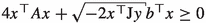
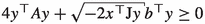
Then, f is hyperbolically convex if and only if

$$\begin{aligned} b_{n+1}+\varphi \left( {\bar{b}},A\right) \ge 0. \end{aligned}$$

In particular, if $A=\textrm{I}$, then f is hyperbolically convex if and only if

$$\begin{aligned} b_{n+1}+\varphi \left( {\bar{b}}\right) \ge 0, \end{aligned}$$

where

Proof

It follows from Proposition 3.6 that f is hyperbolically convex, if and only if

for all ${{\bar{x}}}, {{\bar{y}}} \in {{\mathbb {R}}}^{n}$. The first statement follows after dividing the last inequality by the quantity

and then using the definition of the infimum. The second statement is a particular instance of the first one. $\square$

Corollary 3.10

Let $A=A^\top \in {{\mathbb {R}}}^{(n+1)\times (n+1)}$ be a nonzero matrix, $b\in {{\mathbb {R}}}^{n+1}$, $c\in {{\mathbb {R}}}$, $f:{{\mathbb {H}}}^n\rightarrow {{\mathbb {R}}}$ be defined by $f(p)=p^\top Ap+b^\top p+c$ and $h:{{\mathbb {H}}}^n\rightarrow {{\mathbb {R}}}$ be defined by $h(p)=p^\top Ap$. Then, the following statements hold:

• (i) If $\lambda _{\min }({\bar{A}})+\sigma \ge 2\Vert {\bar{a}}\Vert _{2}$ and $b_{n+1}\ge \Vert {\bar{b}}\Vert _{2}+4\Vert {\bar{a}}\Vert _{2} -2\lambda _{\min }({\bar{A}})-2\sigma ,$ then f is hyperbolically convex. In particular, if $A=\textrm{I}$ and $b_{n+1}\ge \Vert {\bar{b}}\Vert _{2}-4$, then f is hyperbolically convex.

• (ii) If $\lambda _{\min }({\bar{A}})+\sigma \ge 2\Vert {\bar{a}}\Vert _{2},$ then h is hypebolically convex.

Proof

Proof of item (i): By using the notations of Theorem 2 and triangular and Cauchy inequality, we have

Considering that $\lambda _{\min }({\bar{A}})+\sigma \ge 2\Vert {\bar{a}}\Vert _{2}$, we obtain from the last inequality that

(34)

Taking into account that

it follows from (34) that $\varphi \left( {\bar{b}},A\right) \ge \displaystyle -\Vert {\bar{b}}\Vert _{2}+ 2\lambda _{\min }({\bar{A}})-4\Vert {\bar{a}}\Vert _{2}+2\sigma$. Therefore, considering that $b_{n+1}\ge \Vert {\bar{b}}\Vert _{2}+4\Vert {\bar{a}}\Vert _{2}-2\lambda _{\min }({\bar{A}})-2\sigma$, we conclude that $\varphi \left( {\bar{b}},A\right) \ge -b_{n+1}$ or equivalently that $b_{n+1}+\varphi \left( {\bar{b}},A\right) \ge 0$. Hence, applying Theorem 3.2, we obtain that f is hyperbolically convex and the first statement of item (i) is proved. The second statement is an immediate consequence of the first one.

Proof of item (ii): Choose $b_{n+1}\ge \Vert {\bar{b}}\Vert _{2}+4\Vert {\bar{a}}\Vert _{2}-2\lambda _{\min }({\bar{A}})-2\sigma$. It follows from item (i) that f is hyperbolically convex. Then, Corollary 3.2 implies that h is also hyperbolically convex. $\square$

Remark 3.3

Item (ii) of Corollary 3.10 improves item (iii) of [5, Theorem 5.2], where the inequality is strict.

Example 3.2

For the particular case in item (i) of Corollary 3.10, by taking $A=\textrm{I}$ any ${\bar{b}}\in {\mathbb {R}}^n$ and $b_{n+1}\in \left[ {\Vert {\bar{b}}\Vert _{2}}-4,\Vert {\bar{b}}\Vert _{2}\right)$, another large class of hyperbolically convex quadratic functions f with $b\notin {{\mathscr {L}}}$ follows.

Corollary 3.11

Let $n\ge 3$ be an integer, $A=A^\top \in {{\mathbb {R}}}^{(n+1)\times (n+1)}$ be a nonzero matrix, $b\in {{\mathbb {R}}}^{n+1}$, $c\in {{\mathbb {R}}}$, $f:{{\mathbb {H}}}^n\rightarrow {{\mathbb {R}}}$ be defined by $f(p)=p^\top Ap+b^\top p+c$. If f is hyperbolically convex, then

(35)

In particular if f is hyperbolically convex and $A=\textrm{I}$, then

(36)

Proof

We will use the notation of Theorem 3.2. We have $\varphi ({\bar{b}},A)=\inf _{{\mathop {{{\bar{x}}}\not \parallel {\bar{y}}}\limits ^{{{\bar{x}}},{{\bar{y}}}\in {\mathbb {R}}^n}}}\psi ({\bar{x}},{\bar{y}},{\bar{b}},A)$, where

Hence, $\psi ({\bar{x}},{\bar{y}},{\bar{b}},A)\le \zeta ({\bar{x}},{\bar{y}},{\bar{b}},A),$ where

and $\varphi ({\bar{b}},A) \le \inf _{{\mathop {{{\bar{x}}}\not \parallel {{\bar{y}}}}\limits ^{{{\bar{x}}},{{\bar{y}}}\in {\mathbb {R}}^n}}} \zeta ({\bar{x}},{\bar{y}},{\bar{b}},A)\le \zeta ({\bar{x}},{\bar{y}},{\bar{b}},A)$ for any ${\bar{x}},{\bar{y}}\in {\mathbb {R}}^n$ with ${\bar{x}}\not \parallel {\bar{y}}$. Thus, Theorem 3.2 implies

$$\begin{aligned} b_{n+1}+\zeta ({\bar{x}},{\bar{y}},{\bar{b}},A)\ge b_{n+1}+\varphi ({\bar{b}},A)\ge 0. \end{aligned}$$

(37)

Let ${\bar{x}}:=-{\bar{b}}$ and ${\bar{y}}\in {\mathbb {R}}^n$ such that ${\bar{y}}^\top {\bar{a}}=0$, ${\bar{y}}^\top {\bar{b}}=0$ and $\Vert y\Vert _{2}=\Vert b\Vert _{2}$. Then, a simple calculation yields that the right-hand side of equation (35) is $-\zeta ({\bar{x}},{\bar{y}},{\bar{b}},A)$. Hence, (35) follows from (37) and (36) is a simple consequence of (35). $\square$

4 Final Remarks

This paper is a natural continuation of [5], where the study of convexity of homogeneous quadratic functions in hyperbolic spaces was started. In contrast to the Euclidean space, the study of non-homogeneous quadratic functions in the hyperbolic space is more elaborate than the study of homogeneous quadratic functions. In [4], the study of the convexity of quadratic functions on the sphere was conducted, with a specific focus on homogeneous functions. An intriguing investigation that merits further exploration involves characterizing non-homogeneous quadratic functions on the sphere, complementing the findings presented in the paper [4]. It is worth noting that when defining a quadratic function on the sphere and in the hyperbolic space, we rely on the fact that these manifolds are subsets of the Euclidean space. In fact, this kind of study could potentially be extended to manifolds that are subsets of matrix spaces. However, conducting a comprehensive study of convex quadratic functions, or more generally, engaging in convex analysis within a general Riemannian manifold, remains a challenging endeavor.

References

Benedetti, R., Petronio, C.: Lectures on Hyperbolic Geometry. Universitext. Springer-Verlag, Berlin (1992)
Boumal, N.: An introduction to optimization on smooth manifolds. http://sma.epfl.ch/~nboumal/book/index.html (2020)
Cannon, J.W., Floyd, W.J., Kenyon, R., Parry, W.R.: Hyperbolic geometry. In: Flavors of Geometry Mathematical Sciences Research Institute Publications, pp. 59–115. Cambridge University Press, Cambridge (1997)
Ferreira, O.P., Németh, S.Z.: On the spherical convexity of quadratic functions. J. Global Optim. 73(3), 537–545 (2019)
Ferreira, O.P., Németh, S.Z., Zhu, J.: Convexity of sets and quadratic functions on the hyperbolic space. J. Optim. Theory Appl. (2022). https://doi.org/10.1007/s10957-022-02073-4
Finsler, P.: Über das Vorkommen Definiter und Semidefiniter Formen in Scharen Quadratischer Formen. Comment. Math. Helv. 9(1), 188–192 (1936)
Jawanpuria, P., Meghwanshi, M., Mishra, B.: Low-rank approximations of hyperbolic embeddings. In: 2019 IEEE 58th conference on decision and control (CDC), pp. 7159–7164. IEEE (2019)
Keller-Ressel, M., Nargang, S.: The hyerbolic geometry of financial networks. Sci. Rep. 11(1), 1–12 (2021)
Krioukov, D., Papadopoulos, F., Kitsak, M., Vahdat, A., Boguñá, M.: Hyperbolic geometry of complex networks. Phys. Rev. E. 82(3), 036106 (2010)
Marcellini, P.: Quasiconvex quadratic forms in two dimensions. Appl. Math. Optim. 11(2), 183–189 (1984)
Moshiri, M., Safaei, F., Samei, Z.: A novel recovery strategy based on link prediction and hyperbolic geometry of complex networks. J. Complex Netw. 9(4), cnab007 (2021)
Muscoloni, A., Thomas, J.M., Ciucci, S., Bianconi, G., Cannistraci, C.V.: Machine learning meets complex networks via coalescent embedding in the hyperbolic space. Nat. Commun. 8(1), 1–19 (2017)
Nickel, M., Kiela, D.: Learning continuous hierarchies in the lorentz model of hyperbolic geometry. In: International conference on machine learning, pp. 3779–3788. PMLR (2018)
Ratcliffe, J.G.: Foundations of Hyperbolic Manifolds, Graduate Texts in Mathematics, vol. 149, third edn. Springer (2019)
Sharpee, T.O.: An argument for hyperbolic geometry in neural circuits. Curr. Opin. Neurobiol. 58, 101–104 (2019)
Tabaghi, P., Dokmanić, I.: Hyperbolic distance matrices. In: Proceedings of the 26th ACM SIGKDD International Conference on Knowledge Discovery & Data Mining, pp. 1728–1738 (2020)
Ungar, A.A.: Analytic Hyperbolic Geometry and Albert Einstein’s Special Theory of Relativity. World Scientific Publishing Co. Pte. Ltd., Hackensack, NJ (2008)
Vollmer, F.W.: Automatic contouring of geologic fabric and finite strain data on the unit hyperboloid. Comput. Geosci. 115, 134–142 (2018)
Wilson, R.C., Hancock, E.R., Pekalska, E., Duin, R.P.: Spherical and hyperbolic embeddings of data. IEEE Trans. Pattern Anal. Mach. Intell. 36(11), 2255–2269 (2014)
Yamaji, A.: Theories of strain analysis from shape fabrics: a perspective using hyperbolic geometry. J. Struct. Geol. 30(12), 1451–1465 (2008)
Author information
Authors and Affiliations
Corresponding author
Additional information
Communicated by Alexandru Kristály.
Publisher's Note
Springer Nature remains neutral with regard to jurisdictional claims in published maps and institutional affiliations.
Rights and permissions
Open Access This article is licensed under a Creative Commons Attribution 4.0 International License, which permits use, sharing, adaptation, distribution and reproduction in any medium or format, as long as you give appropriate credit to the original author(s) and the source, provide a link to the Creative Commons licence, and indicate if changes were made. The images or other third party material in this article are included in the article's Creative Commons licence, unless indicated otherwise in a credit line to the material. If material is not included in the article's Creative Commons licence and your intended use is not permitted by statutory regulation or exceeds the permitted use, you will need to obtain permission directly from the copyright holder. To view a copy of this licence, visit http://creativecommons.org/licenses/by/4.0/.
About this article
Cite this article
Ferreira, O.P., Németh, S.Z. & Zhu, J. Convexity of Non-homogeneous Quadratic Functions on the Hyperbolic Space. J Optim Theory Appl 199, 1085–1105 (2023). https://doi.org/10.1007/s10957-023-02332-y
Received:
Accepted:
Published:
Issue Date:
DOI: https://doi.org/10.1007/s10957-023-02332-y