
Abstract
We study the abelian sandpile model on a random binary tree. Using a transfer matrix approach introduced by Dhar and Majumdar, we prove exponential decay of correlations, and in a small supercritical region (i.e., where the branching process survives with positive probability) exponential decay of avalanche sizes. This shows a phase transition phenomenon between exponential decay and power law decay of avalanche sizes. Our main technical tools are: (1) A recursion for the ratio between the numbers of weakly and strongly allowed configurations which is proved to have a well-defined stochastic solution; (2) quenched and annealed estimates of the eigenvalues of a product of n random transfer matrices.
1 Introduction
The abelian sandpile model (ASM) is a thoroughly studied model both in the physics and in the mathematics literature see e.g. [3, 4, 9, 12, 15] for recent review papers on the subject. In physics, it serves as a paradigmatic model of self-organized criticality (SOC). SOC is usually referred to as the phenomenon that the model exhibits power law decay of correlations or avalanche sizes, without fine-tuning any external parameters such as temperature or magnetic field. In mathematics, the ASM is connected to several combinatorial objects such as spanning trees, graph-orientations, dimers, and it has an interesting abelian group structure.
The ASM has been studied on the Bethe lattice (i.e., the rootless binary tree) in [5]. Via a recursive analysis, based on a transfer matrix method, the authors in [5] arrive at exact expressions of various quantities of interest, such as the single height distribution, correlation functions of height variables, and avalanche size distribution.
There are various motivations to consider the ASM on random graphs. As an example, we mention integrate-and-fire models in neuroscience (see e.g. [10] and related papers), where the connections between neurons are updated after a neuron has fired. The typical connection structure of a network of firing neurons is therefore generically not translation invariant, and time dependent. As a first approximation, one can quench the randomness of the connection graph and study the firing of neurons on the derived random graph. So far, the ASM model has been studied on small world graphs from the physicist’s perspective, using a renormalization group approach [8]. In the mathematics literature, there are recent studies on so-called “cactus” graphs [7, 13].
In this paper, we start this study of the ASM on random graphs with the ASM on a random tree, for the sake of simplicity chosen to be a realization of a binary branching process with branching probability p∈[0,1]. We use the transfer-matrix method of [5] to express relevant quantities such as the correlation of height variables and the avalanche size distribution in terms of the eigenvalues of an ad hoc product of random matrices. This is the fundamental difference between the Bethe lattice case and the random tree, namely the fact that the transfer matrices depend randomly on the vertices and instead of having to deal with the n-th power of a simple two by two matrix, one has to control the product of n random matrices.
The crucial quantity entering the transfer matrices is the so-called characteristic ratio, which is the ratio between the numbers of weakly and strongly allowed configurations. This ratio is equal to 1 in the infinite Bethe lattice for every vertex and it is close to 1 for vertices belonging to a finite subset of the Bethe lattice which are far away from the “boundary” (see later on for precise statements). In our case, we show that for an infinite random tree the characteristic ratio is a well-defined random variable, uniquely determined by a stochastic recursion. The transfer matrices will then contain elements with that distribution. We also consider deterministic trees that are strict subsets of the binary tree where the characteristic ratio can be computed explicitly. Next, we prove the exponential decay of correlation of height variables (as in the Bethe lattice case), and show that for a branching probability p sufficiently small, but still supercritical (p>1/2), i.e., the branching process survives with positive probability, avalanche sizes decay exponentially. This shows a transition between exponential decay of avalanche sizes, for p small, and power law decay for p close to (possibly only equal to) one.
Our paper is organized as follows. First we recall some basic material about the ASM on trees and the recursive technique developed in [5]. Second we study the recursion for the characteristic ratio and show it has a unique solution for the random binary tree. Finally we give quenched and annealed estimates of the eigenvalues of the product of n random matrices, which we apply in the study of correlation of height variables and avalanche sizes.
2 Abelian Sandpile Model on Subtrees of the Full Binary Tree
We summarize here the basic and standard objects of the abelian sandpile model on a (general) tree. More details can be found e.g. in [5, 11].
2.1 Rooted and Unrooted Random Trees
We denote by  the rooted binary tree of n generations, and by
  the rooted infinite binary tree. For a more general tree
  we write
  if we want to indicate that the tree has root i. The rootless infinite binary tree or Bethe lattice is then obtained by joining two infinite rooted binary trees by a single edge connecting their roots.
A random binary tree of N generations with branching probability p∈[0,1] is a random subset  of
of  obtained as follows. Starting from the root, we add two new vertices, each connected with a single edge to the root (resp. no vertices), with probability p (resp. (1−p)), and we iterate this from every new vertex independently for N generations. By letting N→∞ we obtain the full binary branching process. Joining two independent infinite copies of this process by a single edge connecting their roots creates the rootless random binary tree. This last procedure is of course identical to create the non-random rootless binary tree from non-random rooted binary trees.
2.2 Height Configurations and Legal Topplings
For  a finite subtree of the Bethe lattice, height configurations on
  are elements
  . For
. For  and
and  , η
u
denotes the height at vertex u. A height configuration
, η
u
denotes the height at vertex u. A height configuration  is stable if η
u
∈{1,2,3} for all
is stable if η
u
∈{1,2,3} for all  . Stable configurations are collected in the set
  .
.
For a configuration  , we define the toppling operator
T
u
via
, we define the toppling operator
T
u
via
where Δ is the toppling matrix, indexed by vertices  and defined by

(u,v neighbors in  means that an edge of
  connects u to v). In words, in a toppling at u, 3 grains are removed from u, and every neighbor of u receives one grain.
A toppling at  is called legal if η
u
>3. A sequence of legal topplings is a composition \(T_{u_{n}}\circ\cdots \circ T_{u_{1}} (\eta)\) such that for all k=1,…,n the toppling at u
k
is legal in \(T_{u_{k-1}}\circ\cdots\circ T_{u_{1}} (\eta)\). The stabilization of a configuration
is called legal if η
u
>3. A sequence of legal topplings is a composition \(T_{u_{n}}\circ\cdots \circ T_{u_{1}} (\eta)\) such that for all k=1,…,n the toppling at u
k
is legal in \(T_{u_{k-1}}\circ\cdots\circ T_{u_{1}} (\eta)\). The stabilization of a configuration  is defined as the unique stable configuration
  that arises from η by a sequence of legal topplings.
2.3 Addition Operator and Markovian Dynamics
For  a finite subtree of the Bethe lattice, and for
  , the addition operator is the map
  defined via

where  is such that δ
u
(u)=1 and δ
u
(z)=0 for
is such that δ
u
(u)=1 and δ
u
(z)=0 for  . In other words, a
u
η is the effect of an addition of a single grain at u in η, followed by stabilization.
. In other words, a
u
η is the effect of an addition of a single grain at u in η, followed by stabilization.
The addition operators commute, i.e., a u a v =a v a u . This is the well-known and crucial abelian property of the sandpile model.
The dynamics of the sandpile model is then the discrete-time Markov chain {η(n),n∈ℕ} on  defined via
where X
i
are i.i.d. uniformly chosen vertices of  .
.
Given a stable height configuration η and  , we define the avalanche
Av(u,η) induced by addition at u in η to be the set of vertices in
, we define the avalanche
Av(u,η) induced by addition at u in η to be the set of vertices in  that have to be toppled in the course of the stabilization of η+δ
u
.
that have to be toppled in the course of the stabilization of η+δ
u
.
2.4 Recurrent Configurations and Stationary Measure
The recurrent configurations of the sandpile model form a subset of the stable configurations defined as follows. A configuration  contains a forbidden subconfiguration (FSC) if there exists a subset
  such that for all u∈S, the height in u is less than or equal to the number of neighbors of u in S. The restriction of η to S is then called a FSC. A configuration is allowed if and only if it does not contain a FSC. Recurrent configurations coincide with allowed ones, and are collected in the set
  .
.
We denote by  the set of probability measures on
  . The Markov chain (3) has a unique stationary probability measure
  which is the uniform measure on the set

where δ η is the point mass concentrated on the configuration η.
2.5 Specific Properties of the Sandpile Model on a Tree
In this section, for the sake of self-containdness, we briefly summarize some basic facts from the paper [5] which we need later on. In a subset of the Bethe lattice, the distance between two vertices is defined as the length (i.e., the number of edges) of the shortest path joining them. A vertex is a surface vertex if it has a number of neighbors strictly less than 3.
2.5.1 Weakly and Strongly Allowed Subconfigurations
The class of allowed configurations can be divided into weakly and strongly allowed ones. Let T be a rooted finite tree with root u and extend it with one vertex v and one edge 〈u,v〉. Consider an allowed configuration ξ on T. We put height 1 at vertex v and investigate the derived configuration ξ′ on T∪{v} such that ξ is the restriction of ξ′ to T, and \(\xi'_{v}=1\). If ξ′ has no FSC, then we call ξ strongly allowed on T, otherwise weakly allowed. We give in Fig. 1 an example of weakly and strongly allowed configurations.On one hand, if η u =2, then there exists a forbidden subconfiguration on S={v,u,i 1}. On the other hand, if η u =3, there are no forbidden subconfigurations.

Example of a tree with root u
2.5.2 Characteristic Ratio and Recursion
Let  be a finite tree, rooted or not. A key quantity in the analysis of [5] is the characteristic ratio
 of
of  between weakly and strongly allowed configurations. For the empty tree
  we put x(∅)=0.
For an infinite tree  we say that the characteristic ratio is well-defined if the limit
  exists, where
  is taken along the net of finite subtrees. That is,
  means that for every ε>0, there exists
  a finite subtree of
  such that, for all finite subtrees
  , we have
  .
.
The characteristic ratio satisfies a recursion property both for rooted and unrooted trees:
where T 1,T 2 are two non-intersecting subtrees of the tree T defined as follows. If T=T o is a rooted tree with root o, then T 1,T 2 are obtained by deleting the root o and splitting the tree into two subtrees whose roots are the two descendants of the root o, see Fig. 2.If T is an unrooted tree, we pick one of its edges, 〈u,v〉, we delete this edge and split T into two rooted subtrees T 1 and T 2 whose roots are u and v, see Fig. 3.This recursion (4) holds for finite trees, and by passing to the limit for infinite trees, provided the limits defining x(T),x(T 1),x(T 2) exist. Dhar and Majumdar obtain from (4) that when the distance from the root of T to the nearest surface vertex tends to infinity (what they call “deep in the lattice”), the characteristic ratio x(T) tends to 1. The authors then derive several explicit quantities (such as height probabilities of a vertex u deep in the lattice) by replacing the characteristic ratio by 1.

Example of a tree with root o which splits into T 1 and T 2

Example of a rootless tree which splits into T 1 and T 2
2.5.3 Transfer Matrix Approach
The transfer matrix approach allows to compute the two-point correlation functions and avalanche size distribution. Let u,v be two vertices in the tree at mutual distance n. They determine n+3 subtrees T
1,…,T
n+3, see Fig. 4. The number of allowed configurations when fixing the heights at u and v can then be obtained via a product  of n+3 two by two matrices with elements determined by the characteristic ratios of the subtrees T
1,…,T
n+3 (see Sect. 4 below for the precise form of these matrices).In particular for the Bethe lattice, all the matrices involved in this product are equal to
of n+3 two by two matrices with elements determined by the characteristic ratios of the subtrees T
1,…,T
n+3 (see Sect. 4 below for the precise form of these matrices).In particular for the Bethe lattice, all the matrices involved in this product are equal to  because the characteristic ratios of all the involved subtrees are equal to one. Let
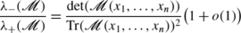
  be a finite or infinite subtree of the full binary tree. The two-point correlation function, i.e., the probability that two vertices u,v at mutual distance n have height i resp. j, for i,j∈{1,2,3}, is equal to (see [5, Sect. 5, Eq. (5.11)])

where  is the ratio of the smallest and largest eigenvalues of the matrix
  and a
i,j
are some numerical constants depending on i,j. For the binary tree,
and a
i,j
are some numerical constants depending on i,j. For the binary tree,  and
and  .
.

Example of a tree with n+3 subtrees
The avalanche size distribution is determined by the inverse of  . For the binary tree, upon addition of a grain at a vertex u, the probability that the avalanche Av(u,η) is a given connected subset
  of cardinality n containing u is equal to

for some constant C, independent of the shape of the subset  . Since there are 4n
n
−3/2(1+o(1)) connected subsets of the Bethe lattice of cardinality n containing u, one concludes that for large n (see [5, Sect. 6, Eqs. (6.13), (6.14)]),
. Since there are 4n
n
−3/2(1+o(1)) connected subsets of the Bethe lattice of cardinality n containing u, one concludes that for large n (see [5, Sect. 6, Eqs. (6.13), (6.14)]),

i.e., the tail of the avalanche size distribution decays like n −3/2.
3 Some Characteristic Ratios
On the Bethe lattice  for the (infinite) rooted subtrees (i=1,2,3) attached to every vertex since every
  is an infinite rooted binary tree (see Sect. 2.5.2). This property considerably simplifies the analysis of [5] and is no longer valid in the inhomogeneous or random cases studied here.
3.1 The Characteristic Ratio of the Random Binary Tree
Let  be the random binary tree of n generations starting from a single individual (the “zero-th” generation) at time n=0 (cf. Sect. 2.1). Then for n>0,
  satisfies the recursive identity [5, Sect. 3, Eq. (3.12)]

where
and  are the (possibly empty) subtrees emerging from the (possibly absent) individuals of the first generation. For a tree
  consisting of a single point we have

because heights 2,3 are strongly allowed and height 1 is weakly allowed (cf. Sect. 2.5.1). This value 1/2 can also be obtained from the recursion (8) by viewing a single point as connected to two empty subtrees (for which x(o)=0). Notice that if u,v∈[0,1], then f(u,v)≤1. Therefore, we view f as a function from [0,1]2 onto [1/2,1].
Lemma 3.1
For every finite subtree
 of the Bethe lattice, the ratio
 . Moreover, on [0,1]2
the function
f
defined by (9) is symmetric, i.e., f(u,v)=f(v,u), and increasing in
u
and
v, i.e., for
u
1≤u
2,
. Moreover, on [0,1]2
the function
f
defined by (9) is symmetric, i.e., f(u,v)=f(v,u), and increasing in
u
and
v, i.e., for
u
1≤u
2,
and analogously in the other argument.
Proof
The proof is straightforward and left to the reader. □
Proposition 3.1
There exists a random variable
X
∞
such that
 in distribution as
n→∞.
in distribution as
n→∞.
Proof
Denote by  the distribution of
  . The recursion (8) induces a corresponding recursion on the distributions
  . We show that
  is a contraction on the set
  of probability measures on [1/2,1] endowed with the Wasserstein distance. This implies that it has a unique fixed point μ
∗ and from every initial μ
0, μ
n
→μ
∗ in Wasserstein distance and thus weakly.
of probability measures on [1/2,1] endowed with the Wasserstein distance. This implies that it has a unique fixed point μ
∗ and from every initial μ
0, μ
n
→μ
∗ in Wasserstein distance and thus weakly.
Let g be a Lipschitz function. Then we have

where T 0,T 1,T 2 are the three trees which cannot be split into two subtrees both non-empty, see Fig. 5.Every other tree T (appearing in the last sum of (12)) can be split into two subtrees both not reduced to a single point. Then using (8), the expression in (12) becomes


The trees T 0,T 1,T 2
Lemma 3.2
The function
 on
on
 defined by

is a contraction on
 endowed with the Wasserstein distance. The contraction factor is bounded from above by 8/9.
Proof
Denote by  the set of Lipschitz functions g:[1/2,1]→ℝ with Lipschitz constant less than or equal to one, i.e., such that |g(x)−g(y)|≤|x−y| for all x,y. We use the following two formulas for the Wasserstein distance of two elements μ,ν of
  [6]:
[6]:


where in the last right hand site the infimum is over all couplings ℙ with first marginal ℙ1 (resp. second marginal ℙ2) equal to μ (resp. ν).
To estimate  we start with the first formula (15)

Now use the definition of f and the fact that x,y∈[1/2,1] to estimate
This gives, using the Lipschitz property of g and a coupling ℙ of μ and ν:

Taking now the infimum over all couplings ℙ, using (16) to bound (18), and taking the supremum over  yields

To estimate the term B(μ,ν,g), use the elementary bound (since x,x′,y,y′∈[1/2,1]):
We then have, using the Lipschitz property of g, and a coupling ℙ′=ℙ′(dxdx′;dydy′) of μ⊗μ and ν⊗ν

Taking the supremum over  , and infimum over the couplings ℙ′, we find

Combining (19), (20) with (17) we arrive at

where in the final inequality we used the elementary bound
□
This proof of Lemma 3.2 completes the proof of Proposition 3.1. □
Remark 3.1
The random binomial tree is such that every vertex has two children with probability p
2, 1 child with probability 2p(1−p) and 0 children with probability (1−p)2, p∈[0,1]. For this case the same idea as in Lemma 3.2 gives a recursion leading to a contraction in the Wasserstein distance and hence  has also a unique limiting distribution.
3.2 The Characteristic Ratio of Some Deterministic Trees
The recursion (8) allows also to compute the characteristic ratio for certain (deterministic) infinite subsets of the full binary tree in terms of iterations of sections of f.
3.2.1 Infinite Branch
First, consider a single branch of length n, i.e., the tree  consisting of a root and n≥1 generations of two individuals each (see Fig. 6).Using (10) we obtain the recursion

which by Lemma 3.1 gives that  is monotonically increasing in n with limit

which is the unique positive solution of

Example of a tree with a single branch of n generations
Remark 3.2
We can generalize this “backbone” tree to a general “backbone-like” tree where at each point the same finite tree T is attached (it is a singleton in the backbone case). The characteristic ratio equals the positive solution of the fixed-point equation
where x(T) denotes the characteristic ratio of the tree T, i.e.,
3.2.2 Finite Perturbations of a Single Branch
Attaching a finite subtree T of the full binary tree  at level n in the infinite single branch
  leads to a tree
  with characteristic ratio

where φ(x)=f(1/2,x) (cf. (23)) is applied n times. This shows that inserting a finite tree T at level n has an effect on the characteristic ratio that vanishes in the limit n→∞, exponentially fast in n.
Moreover, since x(T)≥1/2 and x↦f(x,y) is monotone for all y (by Lemma 3.1), we have from (26)

From (27) and (22) we conclude that for every infinite subtree  for which
  exists,

4 Transfer Matrix and Eigenvalues: Uniform Estimates
In the analysis of the two point correlation function and of the avalanche size distribution, one is confronted with the problem of estimating the minimal and maximal eigenvalues (denoted by  and
and  ) of a product of matrices of the form

with
where the x i ’s are the characteristic ratios of some recursively defined subtrees.
When x i =1 for all i, this exactly corresponds to the analysis in [5] (see the above Sect. 2.5.3). More precisely, in that case, one needs the minimal and maximal eigenvalues (denoted by λ − and λ +) of

which are λ −=1 and λ +=4n. This leads to a decay of the covariance proportional to 1/4n=λ −/λ + and decay of avalanche size asymptotically proportional to
where

denotes the cardinality of the set of connected clusters of size n containing the origin o. In the general case the decay of covariance can be estimated by the ratio  , and for the decay of the avalanche size distribution, one needs to estimate
  as well as the analogue of A
n
. In the case of a branching process, the x
i
’s appearing in the matrix
as well as the analogue of A
n
. In the case of a branching process, the x
i
’s appearing in the matrix  are independent random variables with distribution μ
∗ defined in the proof of Proposition 3.1.
are independent random variables with distribution μ
∗ defined in the proof of Proposition 3.1.
In this section we therefore concentrate on the estimation of the eigenvalues of a matrix of the form  for general x
i
’s.
for general x
i
’s.
Lemma 4.1
-
1.
For all n and all x i ∈[1/2,1] (1≤i≤n), the eigenvalues of
 are non-negative.
 -
2.
We have the inequality
 (31)
(31) -
3.
We have
 (32)
(32)
 are non-negative.

where o(1) tends to zero as n→∞, uniformly in the choice of the x i ’s.
Proof
The eigenvalues are given by

with  and
and  (we abbreviate
  for
for  in these expressions). For n=1, a
2−4b=5+4x≥0. Hence
in these expressions). For n=1, a
2−4b=5+4x≥0. Hence
For n≥2, we estimate, as in [11]

and using

we have
In particular, 4b≤a 2 which implies that the eigenvalues are real and non-negative (a≥0). Inequality (31) then follows from (36), (33).
Given that (by (36)) h=b/a 2 tends to zero as n→∞ at a speed at least C(4/9)n, we have

which proves the third statement. □
Lemma 4.1 shows that the ratio  behaves in leading order as
  . To estimate this ratio, we need to estimate
  from below. We start with a useful representation of
  .
.
Lemma 4.2
Define
Then we have

where y i =(1+x i ) and where

Proof
We have

The result then follows from expansion of this product. □
Lemma 4.3
-
1.
For all n≥1,
$$ E_1^n= \left ( \begin{array}{c@{\quad}c} 1&n\\ 0&1 \end{array} \right ),\qquad E_2^n =E_2, \qquad E_1^n E_2= \left ( \begin{array}{c@{\quad}c} n&n\\ 1&1 \end{array} \right ). $$(40) -
2.
For all r≥1, k 1,…,k r ,k r+1≥0,
$$ \operatorname{Tr} \Biggl(\prod_{i=1}^r \bigl(E_1^{k_i}E_2\bigr) \Biggr)= \prod _{i=1}^r (1+k_i) $$(41)and
$$ \operatorname{Tr} \Biggl( \Biggl(\prod _{i=1}^r \bigl(E_1^{k_i}E_2 \bigr) \Biggr) E_1^{k_{r+1}} \Biggr)= \Biggl(\prod _{i=2}^r (1+k_i) \Biggr) (1+k_1+k_{r+1}). $$(42)
Proof
Identity (42) follows from (41) and invariance of the trace under cyclic permutations. To prove (41), use the expression in (40) for \(E_{1}^{n}E_{2}\), and estimate the diagonal elements of the product
which implies the result. □
Proposition 4.1
For all x 1,…,x n ∈[1/2,1] we have

As a consequence we have the following uniform upper bound

where
Proof
Remember definition (39) of  for α=(α
1,…,α
n
)∈{0,1}n. Using Lemma 4.3 we see that
for α=(α
1,…,α
n
)∈{0,1}n. Using Lemma 4.3 we see that

where  —with the convention α
n+1=1—is the number of intervals of successive 1’s in the configuration α. Hence by( 38) we obtain the lower bound
—with the convention α
n+1=1—is the number of intervals of successive 1’s in the configuration α. Hence by( 38) we obtain the lower bound

Next since \(\sum_{\alpha=(\alpha_{1},\ldots,\alpha_{n})\in\{0,1\} ^{n}} (\prod_{i=1}^{n}(2y_{i})^{\alpha_{i}} )=\prod_{i=1}^{n}(1+2y_{i})=:Z\), we rewrite
where
defines a (y i ) i dependent probability measure on the α’s. Now apply Jensen’s inequality in (46) to obtain

Finally, use y i =1+x i ∈[3/2,2] to estimate
which gives the following uniform lower bound for  :
:

Combining this with  we obtain

Finally we use y i =(1+x i ) with x i ∈[1/2,1] and the fact that x↦(1+x)(3+2x)−1 is increasing to estimate
which implies (44). □
5 Transfer Matrix: Annealed Estimates
In this section we look at the eigenvalues of  where now the x
i
’s are i.i.d. with a law μ on [1/2,1]. We denote by ℙ the joint law of the x
i
’s and by \(\mathbb{E}\) the corresponding expectation.
where now the x
i
’s are i.i.d. with a law μ on [1/2,1]. We denote by ℙ the joint law of the x
i
’s and by \(\mathbb{E}\) the corresponding expectation.
We start with the following lemma.
Lemma 5.1
For all γ≥0 the eigenvalues of
given by
are non-negative.
Proof
Elementary computation. □
Theorem 5.1
Let
 denote the largest, resp. smallest, eigenvalues of
 where the
x
i
’s are i.i.d. with a law supported on [1/2,1]. Denote
where the
x
i
’s are i.i.d. with a law supported on [1/2,1]. Denote

Then we have:
-
1.
Concentration property: there exists C>0 such that for all ε>0
$$ \mathbb{P} \bigl( \bigl(Y_n-\mathbb{E}(Y_n) \bigr)>\varepsilon \bigr)\leq e^{-C\varepsilon^2 n}. $$(49) -
2.
The limits
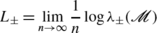 (50)
(50)exist and satisfy \(L_{\pm}=\mathbb{E}(L_{\pm})\) almost surely; moreover
$$ L_++L_-= 2\mathbb{E} \bigl(\log(1+x_1) \bigr). $$(51) -
3.
Upper bound
$$ \lim_{n\to\infty} Y_n=L_+-L_- = \lim_{n\to\infty} \mathbb{E}(Y_n)\leq \log\frac{\varLambda_+ (\gamma)}{\varLambda_- (\gamma)} $$(52)where Λ ± are given by (47) and \(\gamma= (\mathbb{E}((1+x_{1})^{-1}) )^{-1}\in[3/2,2]\).

Proof
We have, using (38)

Using that the weights

are non-negative and sum up to one, we compute the variation

Statement 1 is then an application of the Azuma-Hoeffding inequality. The first part of Statement 2 follows from Oseledec’s ergodic Theorem [14], together with (35) and the law of large numbers. To prove Statement 3, start from (38), (32), and use Jensen’s inequality, combined with the mutual independence of y i =1+x i ,1≤i≤n, to obtain

with \(\gamma^{-1}= \mathbb{E}(y_{1}^{-1})\), and Λ ±(γ) given by (47). Because of (35), we finally derive (51) by the law of large numbers. □
6 Covariance and Avalanche Sizes
6.1 Quenched and Annealed Covariance
Theorem 6.1
Let
 be a finite or infinite subtree of the full binary tree
 . As before, denote by
 the uniform measure on the recurrent configurations
 of the sandpile model on
 and let
 be at mutual distance
n. Then we have the following estimate for the two point correlation function
be at mutual distance
n. Then we have the following estimate for the two point correlation function

In particular,  is absolutely summable, uniformly in the choice of the subtree
 :
:

Proof
The first statement (56) follows from the expression of the covariance in Sect. 2.5.3, Eq. (5), together with Proposition 4.1. Since the number of vertices at distance n in  from the origin is bounded from above by 2n, and γ<1/2, (57) follows from (56). □
Theorem 6.2
Let
 be the stationary binary branching process with reproduction probability
p, conditioned to have a path from its root
o
to a vertex at distance
n. Let
be the stationary binary branching process with reproduction probability
p, conditioned to have a path from its root
o
to a vertex at distance
n. Let
 denote the uniform measure on recurrent configurations on
 . Let
. Let
 denote the covariance of the height variables at
o
and at a vertex
v(n) at distance
n
from the root
o. Then we have the following annealed lower bound on the covariance.
denote the covariance of the height variables at
o
and at a vertex
v(n) at distance
n
from the root
o. Then we have the following annealed lower bound on the covariance.

where \(\gamma^{-1}=\mathbb{E}(y_{1}^{-1})\) and y 1=1+x 1, with x 1 distributed according to the measure of Proposition 3.1, and Λ ± given in (47).
Proof
The result follows from the expression of the covariance in Sect. 2.5.3, Eq. (5), together with (52). □
6.2 Avalanche Sizes
We start by defining a matrix associated to an avalanche cluster. Roughly speaking, the probability that the avalanche coincides with the cluster is the inverse of the maximal eigenvalue of this matrix. Let  be a finite or infinite subtree of the full rootless binary tree, containing the origin o. Let
  be a connected subset of
  containing the origin.
Definition 6.1
Let  . The matrix associated to
  in
in  , denoted by
  is defined as follows. To the vertices in
  are associated n+2 subtrees T
1,…,T
n+2 with corresponding characteristic ratios x(T
i
). Then
are associated n+2 subtrees T
1,…,T
n+2 with corresponding characteristic ratios x(T
i
). Then

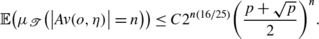
Lemma 6.1
As before, for a stable height configuration
η, let
Av(o,η) denote the avalanche caused by addition of a single grain at the origin in
η, and
 the uniform measure on recurrent configurations
 on
on
 . Then there exist constants
c
1,c
2>0 such that
. Then there exist constants
c
1,c
2>0 such that

where
 is the matrix of (59) associated to
 of Definition 6.1.
Proof
It follows from the expression for  in Sect. 2.5.3, Eq. (6). □
Definition 6.2
We denote by  the number of connected subsets of edges of
  containing the origin o and of cardinality n.
-
1.
The growth rate is defined as
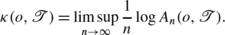 (61)
(61) -
2.
We define the averaged growth rate as


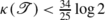
The growth rate gives the dominant exponential factor in the number  . E.g. if
  is the full binary tree, κ=log4, since

see also [5], Sect. 2.5.2. For a stationary binary branching process we have the upper bound

For an exact expression  from which inequality (63) follows immediately, we refer to Appendix, Proposition 7.2.
Theorem 6.3
-
1.
There exists C>0 such that for all n≥1 we have
 (64)
(64)In particular if the tree
 has growth rate
 , then the avalanche size decays exponentially.
 -
2.
For the stationary binary branching tree with branching probability p, we have the estimate
 (65)
(65)In particular, for
$$p< 0.54511\ldots $$the averaged (over the realization of the tree) probability of an avalanche size n decays exponentially in n.
-
3.
For the binomial branching tree we have
 (66)
(66)

 has growth rate
 , then the avalanche size decays exponentially.

In particular, for
the averaged (over the realization of the tree) probability of an avalanche size n decays exponentially in n.
Proof
The first result, i.e., (64), follows from Lemma 6.1, and the estimate (43) which gives the following lower bound on the largest eigenvalue

The second result follows from Lemma 6.1, (67), (63), (62) and Proposition 7.1 below. The solution of
is given by
The l.h.s. of (68) as a function of p is monotone, which yields that for p<0.54511 the expected number of avalanches of size n decays exponentially.
The third statement follows from Lemma 6.1, (67), (63), (62) and Remark 7.1. □
Remark 6.1
From Theorem 6.3 we conclude that avalanche sizes decay exponentially for p small enough. We know that on the full binary tree (corresponding to p=1) avalanche sizes have a power law decay. It is a natural question whether the transition between exponential and power law decay occurs at some unique non-trivial value p c ∈(1/2,1). This question is related to the behavior of a random walk on the full binary tree, killed upon exiting a random subtree. Would this random walk have a survival time with a finite exponential moment, then we would have p c =1. Notice that for the corresponding problem on the lattice ℤd, this random walk does not have a finite exponential moment of its survival time, because the tail of the survival time is stretched exponential (Donsker-Varadhan tail \(e^{-c t^{d/(d+2)}}\)). However, on the tree in the annealed case corresponding to Theorem 6.3, the decay of the tail of the survival time is not straightforward. Formally taking the limit d→∞ in the Donsker-Varadhan tail suggests that on the tree, the survival time of this random walk has a finite exponential moment, which points into the direction p c =1. See also [2] for trapped random walk on a tree.
References
Andrews, G.E., Askey, R., Ranjan, R.: Special Functions. Encyclopedia of Mathematics and Its Applications, vol. 71. Cambridge University Press, Cambridge (1999). ISBN 978-0-521-62321-6
Chen, M., Yan, S., Zhou, X.: The range of random walk on trees and related trapping problem. Acta Math. Appl. Sin. 13, 1–16 (1997)
Dhar, D.: Theoretical studies of self-organized criticality. Physica, A 369, 29–70 (2006)
Dhar, D.: Self-organized critical state of sandpile automaton models. Phys. Rev. Lett. 64, 1613–1616 (1990)
Dhar, D., Majumdar, S.N.: Abelian sandpile model on the Bethe lattice. J. Phys. A, Math. Gen. 23, 4333–4350 (1990)
Dudley, R.M.: Real Analysis and Probability. Cambridge University Press, Cambridge (2002)
Gauthier, G.: Avalanche dynamics of the Abelian sandpile model on the expanded cactus graph. Preprint (2011). Available at http://arxiv.org/abs/1110.6263
Goh, K.I., Lee, D.S., Kahng, B., Kim, D.: Sandpile on scale-free networks. Phys. Rev. Lett. 91, 148701 (2003)
Járai, A.A.: Thermodynamic limit of the abelian sandpile model on ℤd. Markov Process. Relat. Fields 11, 313–336 (2005)
Levina, A., Herrmann, J.M., Geisel, T.: Dynamical synapses causing self-organized criticality in neural networks. Nat. Phys. 3, 857–860 (2007)
Maes, C., Redig, F., Saada, E.: The Abelian sandpile model on an infinite tree. Ann. Probab. 30, 2081–2107 (2002)
Maes, C., Redig, F., Saada, E.: Abelian sandpile models in infinite volume. Sankhya, 67 (4), 634–661 (2005)
Matter, M., Nagnibeda, T.: Abelian sandpile model on randomly rooted graphs and self-similar groups. Preprint (2010). Available at http://arxiv.org/abs/1105.4036
Osedelec, V.L.: A multiplicative ergodic theorem: Lyapunov characteristic number for dynamical systems. Trans. Mosc. Math. Soc. 19, 197–231 (1968)
Redig, F.: Mathematical aspects of the abelian sandpile model. In: Mathematical Statistical Physics, Les Houches Summer School, pp. 657–729. Elsevier, Amsterdam (1989)
Temme, N.M.: Special Functions: An Introduction to the Classical Functions of Mathematical Physics. Wiley, New York (1996). ISBN 0-471-11313-1
Acknowledgements
We would like to thank Remco van der Hofstad for useful discussions. F.R. and W.M.R. thank NWO for financial support in the project “sandpile models in neuroscience” within the STAR cluster. This work was supported by ANR-2010-BLAN-0108 and by NWO. We also thank laboratoire MAP5 at Université Paris Descartes, Universities of Leiden and Delft for financial support and hospitality.
Open Access
This article is distributed under the terms of the Creative Commons Attribution License which permits any use, distribution, and reproduction in any medium, provided the original author(s) and the source are credited.
Author information
Authors and Affiliations
Corresponding author
Appendix: The Expected Number of Clusters Containing the Origin in a Random Binary Tree
Appendix: The Expected Number of Clusters Containing the Origin in a Random Binary Tree
Proposition 7.1
Let
p
be the probability that a vertex has 2 children. Furthermore let
 denote the number of connected clusters of
n
edges containing
o, given a realization of a tree
denote the number of connected clusters of
n
edges containing
o, given a realization of a tree
 with root
o. Then there exists a constant
C>0 such that for
n≥1 we have
with root
o. Then there exists a constant
C>0 such that for
n≥1 we have

Remark 7.1
For the binomial branching tree, where every vertex has 2 children with probability p 2 and 1 child with probability 2p(1−p) (see Remark 3.1), we have the upper bound

which follows from the observation that the number of n vertex animals containing the root of the full binary tree is bounded from above by 4n, and in the case of binary branching tree, each of these vertices is present with probability p independently, which gives the factor p n.
Proof
If we define a n to be the expected number of connected clusters containing o and with n vertices, then a n satisfies the recursion relation

Furthermore, by definition we put a 0=1. Thus, going from vertices to edges,

Introduce then the associated generating function:

For \({x\in [0,\frac{-p+\sqrt{p}}{2p(1-p)} ]}\), this power series is convergent and, using A(0)=1, it is given by
for \(x\in (0,\frac{-p+\sqrt{p}}{2p(1-p)} ]\). Use (for z such that 4z<1)
to obtain
We put k=n+j, then n=k−j and j≤n+1 yields j≤⌊(k+1)/2⌋, hence the expected number of clusters a k containing the origin is equal to
where

with c=(1−p)/p. All terms in the sum (78) are exponentially large in k, hence the exponential growth of the sum is determined by its maximal term. Using Stirling’s approximation \(n! \approx n^{n} e^{-n}\sqrt{2\pi n}\) for the right hand side of (79), we obtain the upper bound
Define, for x∈[0,(k+1)/2],
This function φ attains its maximum at \(x= k(1-\sqrt{p})/2\), which combined with (80), implies
Plugging (81) into (78) and bounding from above induces (70). □
In the following proposition we give an exact formula for  .
.
Proposition 7.2
We have the following identity,

where 2 F 1(⋅,⋅,⋅,⋅) denotes the hypergeometric function defined as
and where the Pochhammer symbol (a) n is defined by
Proof
Let us first remark that for |z|<1, real a,b and c≠−m where m∈ℕ, the series in (83) is well defined. In our case z=−(1−p)/p, a=−(n+1)/2, b=1/2−(n+1) and c=(n+1)−1/2 ( see also [1] for more details about the hypergeometric function). The claim (82) follows from (73) and (78) once we show the identity

If a or b are negative integers, using (84) we see that the series (83) defining 2 F 1 is a finite sum. Therefore,

We have
Next we use the functional identities for the Gamma function (see [16]),
and recurrence relation
to rewrite
in terms of Gamma functions with positive arguments. Thus

which gives
with
and
Furthermore expanding numerator and denominator of this expression gives B=(−1)j. To rewrite A, we use (89) and the duplication formula
once for z=(k+1)/2:

and another time for z=(k+1)/2−j:

Hence
and since the Catalan numbers satisfy
we can write

which is equal to
and yields the claim. □
Remark 7.2
For p=1, we recover the classical formula for the number of animals of n edges containing the origin in a binary tree (cf. Sect. 2.5.2):

for some constant C.
Proof
This follows from the fact that for p=1, 2 F 1(a,b,c,0)=1. □
Rights and permissions
Open Access This article is distributed under the terms of the Creative Commons Attribution 2.0 International License (https://creativecommons.org/licenses/by/2.0), which permits unrestricted use, distribution, and reproduction in any medium, provided the original work is properly cited.
About this article
Cite this article
Redig, F., Ruszel, W.M. & Saada, E. The Abelian Sandpile Model on a Random Binary Tree. J Stat Phys 147, 653–677 (2012). https://doi.org/10.1007/s10955-012-0498-6
Received:
Accepted:
Published:
Issue Date:
DOI: https://doi.org/10.1007/s10955-012-0498-6