
Abstract
Some ground state properties of a fermion system are investigated. An initial Hamiltonian being a generalization of the lattice Anderson model describes this system as a two-band electron-phonon one where both of electron bands are narrow (one is wider than the other). Two bands are hybridized and electrons from both of them are strongly coupled to the same local phonons. After performing the Lang–Firsov type transformation, a new polaron Hamiltonian is obtained. As a result, there appear three effective polaron-polaron interactions in this Hamiltonian and the bandwidths of both of electron bands are reduced. It is assumed that the reduction of the bandwidth of one of the bands is sufficiently strong to make this band dispersionless. Each of the interactions can lead to superconductivity on its own but only one of them is taken into account at this stage; it is the interaction between electrons from the band with a dispersion. The Bogolyubov’s mean field approach is used in order to find the spectrum of the reduced effective Hamiltonian. The effect of the hybridization on the superconducting gap and the relationship between the critical hybridization and the average number of electrons from the wider band per lattice site are investigated.
1 Introduction
The investigations of two-band electron systems have long history. Especially, this concerns superconductivity. The early papers [1, 2] dealt with a two-band superconductor in which apart from conventional BCS interactions acting inside bands there is another potential describing the transitions of Cooper pairs between different bands. In other words, there is a possibility of the mutual tunneling of Cooper pairs from one band to the other. It turns out that the presence of such an interaction can result, for instance, in the enhance of the critical temperature [3].
Some research was done on the grounds of the Anderson lattice model (ALM) to which attractive interactions between electrons were incorporated. Hamiltonians created in this way serve very frequently as the models of superconducting heavy-fermion systems [4, 5] or mixed-valence compounds [6–8]. In the former case, the wider band can be occupied, for instance, by d-electrons whereas the narrower one by f-electrons. f-electrons repel each other while an interaction between d-electrons is attractive. Additionally, there is a mixing term hybridizing both of bands. The compound Nd2−x Ce x Cu4 can be a good example of such a system. In the latter case, one can list a lot of compounds in which so-called local electron pairs can exist. For example, V3Si, Nb3Ge, and BaBi x Pb1−x O3 can be mentioned. In these systems, electrons from the narrower band attract each other. This makes electron pairs appear in this band in such a system. Some lattice sites are empty while others are occupied by these pairs. Depending on the strength of the binding potential conventional Cooper pairs or local bipolarons occur. In the latter case, local bipolarons resemble more local lattice bosons than conventional Cooper pairs.
Another way to investigate the superconductivity in a two band system is to deal with so-called Kondo lattices. Obviously, the Kondo lattice model (KLM) can be derived from ALM by making use of the Schrieffer–Wolf transformation; however, some researchers take KLM as a starting point of considerations [9]. In such a case, conduction electrons interact with localized ones via the spin exchange interaction. The interaction leads to antiferromagnetic coupling of spins of electrons from both bands resulting in the competition between superconductivity, magnetically ordered phases and the Kondo effect.
The Anderson and the Kondo lattice models frequently serve to describe the so-called concentrated alloys. To describe superconducting dilute alloys, the s-d model or one-impurity Anderson model are invoked; see, e.g., [10]. Recently, a BCS system with magnetic impurities in the frame of the s-d model has been investigated [11]. One of the findings was the coexistence of ferromagnetism and superconductivity in some range of parameters. Moreover, the comparison of the theory predictions with some experimental results concerning some reentrant superconductors was made and gave the very good agreement between them.
Some of the topics mentioned above are discussed in more detail in the book by Hewson [12]
In this paper, we would like to investigate a two-band electron system at zero temperature. Initially, we start with a electron-phonon Hamiltonian being in fact an extended form of the Anderson lattice model. We assume that electrons fill two narrow bands that could be of the d and the f character. They interact not only with one another but with the same local bosons as well. This assumption is quite reasonable as these bands are always narrow relative to the s or the p bands. This Hamiltonian is transformed by making use of a Lang–Firsov type transformation to a new two-band polaronic Hamiltonian. As a result, one obtains three local effective electron-electron interactions: two intraband and one interband. Furthermore, the hopping integrals and the hybridization parameter V are exponentially reduced. It is assumed that one of the bands has the bandwidth so much reduced to be actually dispersionless. The Hamiltonian obtained in this way can describe different physical situations depending on the character of those three electro-electron potentials. For example, if the interaction in the narrower band is repulsive then the system represents a heavy-fermion system. Such a system will become superconducting if electrons from the wider band attract each other. In turn, if the potential acting in the dispersionless band changes its character to be attractive then superconductivity can occur in the system. This type of superconductivity was called bipolaronic superconductivity since bipolarons are responsible for this phenomenon. As was already mentioned in the text, bipolarons resemble Cooper pairs or local heavy bosons depending on the strength of the coupling constant [6].
In this work, we would like to investigate a case which lies between these two situations. This consists in putting the interaction in the dispersionless band equal zero. Additionally, we assume that the interband potential is zero, also. The only nonzero interaction is that acting in the wider band and is assumed to be attractive so one deals with a two band superconductor. This means that dispersionless electrons with opposite spins need not avoid each other when getting the same lattice site. As one can see, there can be double, single, and empty occupancies in this band. The derivation of the effective mean field Hamiltonian is a subject of Sect. 2. In Sect. 3, the spectrum of this Hamiltonian is found and the ground state vector and the corresponding energy is identified. In Sect. 4, the properties of the system in the ground state are investigated. Especially, this concerns the influence of the mixing term and the position of the dispersionless band on the superconducting order parameter (the superconducting gap). At the end, the outline of the thermodynamics is presented. Expressions for the free energy per lattice site, the superconducting gap and the chemical potential are derived. However, the resulting formulas are too complex to be put under analytical treatment. This is so even in the simplest case corresponding to the shift of the dispersionless band to the Fermi level.
This work stands for only preliminary step in investigations of the initial Hamiltonian and moreover poses a different point of view since such problems are frequently treated within the Green’s function approach. The comparison with experiment is not performed here. Moreover, magnetic phenomena are absent as well but this is actually a logical consequence of the lack of the repulsion in the dispersionless band. Such a repulsion can be incorporated into calculations by means of mean field method [4] or perturbation theory. These problems and others will be handled in future works.
2 The Model
Our starting point is the following Hamiltonian:


\(c_{i\sigma}^{\ast}\) and c iσ represent the creation and annihilation operators of an electron from the wider band (called the c band from now on) whereas \(d_{i\sigma}^{\ast}\) and d iσ concern electrons from the narrower one (called the d band from now on), respectively. σ denotes the spin of electrons and i and j refer to lattice sites. \(n_{i\sigma}^{d}\) and \(n_{i\sigma}^{c}\) are the number operators of both kinds of electrons. \(b_{i}^{\ast}\) and b i are the creation and annihilation operators of a local phonon. \(t_{ij}^{c}\) and \(t_{ij}^{d}\) denote the hopping integrals of electrons from the c and d bands, respectively. This means that \(|t_{ij}^{c}|\gg |t_{ij}^{d}|\) is assumed. E c and E d refer to the site energies of both kinds of electrons, respectively. V is the conventional on-site hybridization and the parameters U c, U d, and U cd are the Coulomb interactions between electrons of the same type and the different types, respectively. Going further, ω is the Einstein oscillations frequency and μ is the chemical potential. Finally, the parameters g c and g d are the electron-phonon couplings. Hamiltonian (2.1) represents a generalized Anderson lattice model in which electrons from both of bands are strongly coupled to the same local phonons and to each other through the Coulomb interactions. The assumption on coupling both types of electrons to the same phonons can lie in the fact that deeper lying bands are always narrower than the s or the p bands. For instance, this concerns the d or the f-bands.
Now we would like to transform this Hamiltonian to a new one expressed in terms of small polarons similarly as it was made, e.g., in [6]. To this end, let us use a Lang–Firsov type transformation

Owing to this transformation the electron-lattice terms can be eliminated to all orders in the coupling constants. One obtains

The Hamiltonian above has now the hopping and hybridization terms modified by exponential factors involving the lattice deformation. To deal with these terms, let us average the Hamiltonian (2.6) over the unperturbed phonon eigenstates of \(H_{ph}=\hbar\omega\sum _{i}b_{i}^{\ast}b_{i}\) and neglect the energy of phonons in analogy to that done in [6]. Therefore, these terms are

and
where \(\beta=\frac{1}{kT}\), the coupling constant g equals g c in the case of hopping of c electrons, g d in the case of hopping of d electrons whereas ±(g c−g d) for the hybridization terms. The approximation used in the above expressions is justified by the inequality kT≪ω which is true at low temperatures. One can notice the exponential reduction of the hopping integrals and the hybridization. Moreover, the site energies and the Coulomb interactions are also modified, namely

There appears a possibility of the formation of electron pairs in both of bands separately as well as mixed pairs of electrons. All electrons are dressed by the lattice deformations and form so called small polarons. If the electron-phonon interactions are sufficiently strong, the effective interactions between electrons get attractive. Of course, if at least one of the Coulomb repulsions has its value sufficient to make the corresponding effective polaron-polaron interaction only weakly attractive then the small polarons bind into something resembling conventional Cooper pairs. When at least one of the coupling constants of these effective interactions is much less than zero local pairs of polarons are formed and they are called local bipolarons. The local bipolarons behave more like local bosons on a lattice. Ultimately, the effective Hamiltonian is

where \(\tilde{t}_{ij}^{c}=t_{ij}^{c} e^{-\frac{{g^{c}}^{2}}{\omega^{2}}}\), \(\tilde {t}_{ij}^{d}=t_{ij}^{d} e^{-\frac{{g^{d}}^{2}}{\omega^{2}}}\) and \(\tilde {V}=Ve^{-\frac{(g^{c}-g^{d})^{2}}{2\omega^{2}}}\). Beside the hybridization there is another term linking two bands, namely, the interband density-density interaction. If this interaction is attractive, there appear pairs formed of two types of electrons. Mixed pairs with opposite and the same spins contribute to the investigated system. The pairs with the same spins could be of significance if they were of the p-wave pairing symmetry. A scenario with mixed pairs was already taken into account to investigate their role in the isotope effect [13]. Generally speaking, different situations can occur. For instance, a next possibility can be the introducing of the repulsion between d electrons that could lead us towards the Kondo lattice system and the interplay between magnetism and superconductivity.
In this paper we postpone the investigation of the Hamiltonian \(\tilde {H}_{\mathrm{eff}}\) in its general form to future papers. Now, we are interested in a less ambitious task, namely, we would like to put \(\tilde {U}^{d}=\tilde{U}^{cd}=0\), \(\tilde{t}_{ij}^{d}=0\) and \(\tilde{U^{c}}<0\). This can be substantiated by the assumption that the coupling between phonons and narrower band electrons is strong enough to reduce hopping of these electrons to zero and to diminish the mentioned effective coupling constants to be negligibly small. The resulting Hamiltonian is

At this stage, it is convenient to pass from the real space representation to the reciprocal space one. Making use of \(c_{i\sigma }^{\ast}=\frac{1}{\sqrt{L}}\sum_{\mathbf{k}}e^{-i\mathbf{k}\mathbf {R}_{i}}c_{\mathbf{k}\sigma}^{\ast}\) and \(d_{i\sigma}^{\ast}=\frac{1}{\sqrt {L}}\sum_{\mathbf{k}}e^{-i\mathbf{k}\mathbf{R}_{i}}d_{\mathbf{k}\sigma }^{\ast}\), where L denotes the number of lattice sites and the vector R i stands for the position of the ith site, one obtains

where \(\xi_{{\mathbf{k}}}^{c}=\varepsilon_{{\mathbf{k}}}+\tilde{E}^{c}-\mu\), \(\xi ^{d}=\tilde{E}^{d}-\mu\), \(n_{{\mathbf{k}}\sigma}^{c}=c_{{\mathbf{k}}\sigma}^{\ast}c_{{\mathbf{k}}\sigma,}\) and \(n_{{\mathbf{k}}\sigma}^{d}=d_{{\mathbf{k}}\sigma}^{\ast}d_{{\mathbf{k}}\sigma}\). Since we would like to address the two-dimensional system with the square lattice with \(t_{ij}^{c}=-t\) for j=i+1 or j=i−1 and \(t_{ij}^{c}=0\), otherwise \(\varepsilon_{\mathbf{k}}=-2te^{-\frac {{g^{c}}^{2}}{\omega^{2}}}(\cos{k_{x}}+\cos{k_{y}})\) is assumed. Moreover, it is superconductivity what we are interested in and we put \(\tilde{U}^{c}<0\). The Hamiltonian above is still very complicated and needs some simplification. One can resort to the well-known BCS approximation and then the Bogolyubov’s mean field one. Finally, it yields

with the gap parameter

The average \(\langle A\rangle_{\tilde{H}_{\mathrm{red}}}=\frac{\mathrm{Tr}\,A e^{-\beta \tilde{H}_{\mathrm{red}}}}{\mathrm{Tr}\,e^{-\beta\tilde{H}_{\mathrm{red}}}}\), where A is an arbitrary operator. This Hamiltonian describes a system with the narrow band of c electrons and the band of d electrons reduced to the dispersionless form. For convenience, we put \(\tilde{E}^{c}=0\) throughout the paper. A similar mean field Hamiltonian with a renormalized hybridization parameter due to the Coulomb repulsion between f electrons was described in [4] where its some fundamental features concerning the \(\tilde{V}\ll\Delta\) regime were investigated. It is worthwhile to add a remark that such a renormalized Hamiltonian may be treated by the utilization of the method introduced in the next section. It is now obvious that the Hamiltonian (2.9) can be diagonalized in each k-subspace separately. This is made in the next section.
3 The Spectrum of the Mean Field Hamiltonian
The Hamiltonian \(\tilde{H}_{{\mathbf{k}}\mathrm{red}}\) in (2.9) acts in a 16-dimensional space \(\mathcal{M}_{\mathbf{k}}\) spanned by \(|n_{1}n_{2}\overline{m}_{1}\overline{m}_{2}\rangle :=(c_{\mathbf{k}+}^{\ast})^{n_{1}}(c_{-\mathbf{k}-}^{\ast})^{n_{2}}\times (d_{\mathbf{k}+}^{\ast})^{m_{1}}(d_{-\mathbf{k}-}^{\ast})^{m_{2}}|0\rangle \), where n i =0,1 and m i =0,1 for i=1,2. The diagonalization of this Hamiltonian leads to the problem of the diagonalization of a 16×16 matrix and thus a formidable task. However, if one defines the operator \(\varLambda_{{\mathbf{k}}}:=n_{{\mathbf{k}}+}^{c}-n_{-{\mathbf{k}}-}^{c}+n_{{\mathbf{k}}+}^{d}-n_{-{\mathbf{k}}-}^{d}\) then the following commutation relation is satisfied
This fact enables us to simplify the problem to the diagonalization of the Hamiltonian in invariant subspaces of \(\mathcal{M}_{{\mathbf{k}}}\). The structure of \(\mathcal{M}_{{\mathbf{k}}}\) is as follows:
-
(A)
There are two 1-dimensional common subspaces \({\mathcal{M}}_{{\mathbf{k}}i}\) (i=1,2) of the operator Λ k i \(\tilde{H}_{{\mathbf{k}}\mathrm{red}}\). They are spanned, respectively, by the following two vectors with the corresponding eigenvalues λ and E k of this operators equal as follows:
-
1.
\(|10\overline{1}\overline{0}\rangle \), λ=2, \(E_{{\mathbf{k}}}=\xi _{{\mathbf{k}}}^{c}+\xi^{d}\)
-
2.
\(|01\overline{0}\overline{1}\rangle \), λ=−2, \(E_{{\mathbf{k}}}=\xi _{{\mathbf{k}}}^{c}+\xi^{d}\)
-
1.
-
(B)
There are also two 4-dimensional common subspaces \({\mathcal{M}}_{{\mathbf{k}}i}(i=3,4)\) of Λ k and \(\tilde{H}_{{\mathbf{k}}\mathrm{red}}\) spanned by the following quartets of vectors \(|n_{1}n_{2}\overline{m}_{1}\overline{m}_{2}\rangle \) with eigenvalues of these operators equal as follows:
-
3.
\(|10\overline{0}\overline{0}\rangle \), \(|00\overline {1}\overline{0}\rangle \), \(|11\overline{1}\overline{0}\rangle \), \(|10\overline {1}\overline{1}\rangle \), λ=1, \(E_{{\mathbf{k}}3}^{j}\), j=1,2,3,4
-
4.
\(|01\overline{0}\overline{0}\rangle \), \(|00\overline {0}\overline{1}\rangle \), \(|11\overline{0}\overline{1}\rangle \), \(|01\overline {1}\overline{1}\rangle \), λ=−1, \(E_{{\mathbf{k}}4}^{j}\), j=1,2,3,4
where
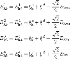
with
$$E_{\mathbf{k}m}=\sqrt{{\xi_{\mathbf{k}}^c}^2+{\xi^d}^2+\Delta^2+2\tilde {V}^2-E_{\mathbf{k}\mathrm{in}}},$$$$E_{\mathbf{k}n}=\sqrt{{\xi_{\mathbf{k}}^c}^2+{\xi^d}^2+\Delta^2+2\tilde {V}^2+E_{\mathbf{k}\mathrm{in}}},$$$$E_{{\mathbf{k}}\mathrm{in}}=\sqrt{{\xi_{\mathbf{k}}^c}^4+{\xi^d}^4+\Delta^4-2{\xi_{\mathbf{k}}^c}^2{\xi ^d}^2+2{\xi_{\mathbf{k}}^c}^2\Delta^2-2{\xi^d}^2\Delta^2+4{\xi_{\mathbf{k}}^{c2}}\tilde{V}^2+8{\xi_{\mathbf{k}}^c}\xi^d\tilde{V}^2+4{\xi^d}^2\tilde {V}^2+4\Delta^2\tilde{V}^2}.$$The eigenvectors of \(\tilde{H}_{{\mathbf{k}}\mathrm{red}}\) in these subspaces have the form
$$\bigl|E_{{\mathbf{k}}3}^j\bigr\rangle =a_{{\mathbf{k}}}^j|10\overline{0}\overline {0}\rangle +b_{{\mathbf{k}}}^j|00\overline{1}\overline{0}\rangle +c_{{\mathbf{k}}}^j|11\overline{1}\overline{0}\rangle +d_{{\mathbf{k}}}^j|10\overline {1}\overline{1}\rangle $$and
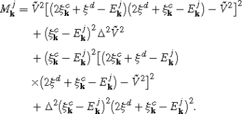
$$\bigl|E_{\mathbf{k}4}^j\bigr\rangle =a_{\mathbf{k}}^j|01\overline{0}\overline {0}\rangle +b_{\mathbf{k}}^j|00\overline{0}\overline{1}\rangle +c_{\mathbf{k}}^j|11\overline{0}\overline{1}\rangle +d_{\mathbf{k}}^j|01\overline {1}\overline{1}\rangle .$$The squared components are the same for these subspaces and take the following form:
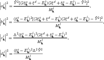
and
-
3.
-
(C)
There is one 6-dimensional common subspace \({\mathcal{M}}_{{\mathbf{k}}5}\) of Λ k and \(\tilde{H}_{{\mathbf{k}}\mathrm{red}}\) spanned by the vectors \(|00\overline {0}\overline{0}\rangle \), \(|11\overline{0}\overline{0}\rangle \), \(|00\overline{1}\overline{1}\rangle \), \(|01\overline{1}\overline{0}\rangle \), \(|10\overline{0}\overline{1}\rangle \), \(|11\overline{1}\overline{1}\rangle \). The eigenvalue of Λ k in \({\mathcal{M}}_{{\mathbf{k}}5}\) is λ=0, whereas the Hamiltonian has the following eigenvalues:
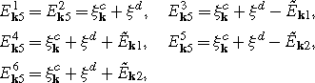
where
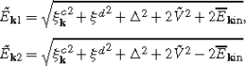
and
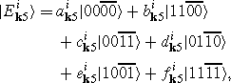
$$\overline{E}_{\mathbf{k}\mathrm{in}}=\sqrt{{\xi_{\mathbf{k}}^c}^2{\xi^d}^2+\Delta ^2{\xi ^d}^2-2\xi_{\mathbf{k}}^c\xi^d\tilde{V}^2+\tilde{V}^4}.$$The eigenvectors in this subspace for i=1,2,3,4,5,6 are:
 (3.1)
(3.1)where the squared components take the following form:
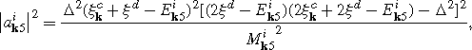 (3.2)
(3.2)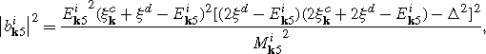 (3.3)
(3.3) (3.4)
(3.4)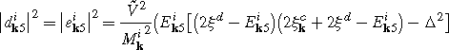 (3.5)
(3.5) (3.6)
(3.6)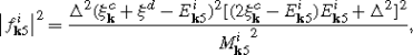 (3.7)
(3.7)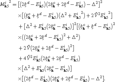 (3.8)
(3.8)


The spectrum is quite complicated but one can recognize the ground state energy and the corresponding vector relatively easy. The lowest energy state vector belongs to the subspace \(\mathcal{M}_{\mathbf{k}5}\) and its number is i=3. Therefore, the ground state energy is \(E_{\mathbf{k}5}^{3}\). This vector has a much more complicated form than the conventional BCS ground state vector. As one can see the structure of the ground state reveals some interesting features since it incorporates states occupied by both different pairs of electrons and the quartet built of two types of pairs.
4 The Ground State Properties
In preceding section, the spectrum of the mean field Hamiltonian was shown. Now let us have a closer look at the ground state. We already know that the ground state vector is \(|E_{\mathbf{k}5}^{3}\rangle \). From now on, we introduce the new notation for this vector, namely, |G k 〉. The total ground state vector is ∏ k |G k 〉=:|G〉. Moreover, we will use the symbols V and U instead of \(\tilde{V}\) and \(\tilde{U}^{c}\) in the following text, respectively. The total ground state energy reads
The equation for the gap parameter at zero temperature can be obtained from the definition (2.10) or from
Furthermore, the equation for the chemical potential μ is needed and this parameter can be determined from
Since we want to investigate the system in the thermodynamic limit (L→∞), it is reasonable to approximate the exact density of states (DOS) for c electrons by making use of

where De denotes the effective bandwidth of the c band. This form of DOS is a good approximation of the exact one in the case of 2-dimensional systems. The equations for Δ and μ now are as follows:

and finally the ground state energy per lattice site is
n is the average number of electrons per lattice site. The above expressions contain integrals that cannot be integrated in a simple way. We will deal with them numerically. Let us add that \(\tilde{E}_{1}\) and \(\overline{E}_{\mathrm{in}}\) are defined in Sect. 3. Our aim is to find the relationship between the gap parameter and the hybridization |V| for different values of the energy E d which is measured from the bottom of the c band. The parameters used for the calculations are as follows: \(\frac{|U|}{\mathit{De}}=0.3\), De=0.1 eV. In Fig. 1, one can see the curves depicting this relationship for the chemical potential \(\mu=\frac {\mathit{De}}{2}\). All the curves represent decreasing functions of the hybridization |V|. If the d band lies below the bottom of the c band, the hybridization has to be of order of De/2 to destroy superconductivity. As the d band is shifted upward, the hybridization becomes more destructive to superconductivity. This should be understood in the sense of how large the critical value of hybridization |V c | is. The critical hybridization is to be meant as the value for which Δ=0. The smallest value of this parameter corresponds to the case with \(E^{d}=\mu=\frac{\mathit{De}}{2}\) (the half-filled case). This means that the hybridization has then the strongest influence on superconductivity. As was mentioned in Introduction, the important thing is not only the question of mechanisms leading to amplifying superconductivity but the problem of factors weakening this phenomenon as well. Here, we can notice two such factors which can affect superconductivity—the hybridization and the position of the d band with respect to the bottom of the c band. When looking at the convexity of these curves, one can notice some crossover from simple behavior for \(E^{d}=\frac{\mathit{De}}{2}\) to much more complicated one for \(E^{d}=-\frac{\mathit{De}}{10}\).

The curves representing the dependence of the superconducting gap on the hybridization parameter |V| for \(\mu=\frac{\mathit{De}}{2}\) and different positions of the d band with respect of the bottom of the c band are depicted
In Fig. 2, the average number of electrons per lattice site versus the hybridization |V| for different values of E d and \(\mu=\frac {\mathit{De}}{2}\) is depicted. When E d=μ, this number equals 2 and does not change with |V|. For lower positions of the d band it is seen that the number n decreases from 3 to 2 when |V| increases. This passing takes place at |V c |. This can be interpreted as follows. When the hybridization is absent, the d orbital at every lattice site is occupied by two electrons and the c band is half-filled. As the hybridization is turned on and increases all d orbitals cannot be fully occupied by two electrons any longer for \(\mu=\frac{\mathit{De}}{2}\) and the filling of the d band diminishes due to the migration of d electrons to the half-filled c band.

The curves representing the dependence of the average number of electrons per lattice site on the hybridization parameter |V| for \(\mu=\frac{\mathit{De}}{2}\) and different positions of the d band with respect of the bottom of the c band are presented
If we admit ξ d=0 from the very beginning, the calculations become much easier. The d band lies now on the Fermi level and the chemical potential is not fixed contrary to that assumed before. The squared components of the ground state vector take the following form:

The gap equation (4.2) takes the form

whereas n=2. It would be interesting to find out how electrons fill the d band and the c band for different values of |V|. To this end, let us calculate the numbers of d and c electrons in the ground state, namely

then in the thermodynamic limit we obtain

Of course, n c+n d=n. The ground state energy per lattice site reads

After making use of (4.6), one obtains

At this stage, it is visible that the hybridization lowers the ground state energy. The hybridization creates a gap in the spectrum of the investigated system.
Especially interesting are three following cases: μ=0, μ=De and \(\mu=\frac{\mathit{De}}{2}\). In the first case, we get

The critical value of the hybridization |V c | can be obtained from the equation for Δ when putting Δ=0. One gets
For μ=De, the expressions for Δ and |V c | are the same as above but \(n^{c}=1-\frac{1}{\mathit{De}}(\sqrt{\Delta^{2}+4V^{2}} -\sqrt {\mathit{De}^{2}+\Delta ^{2}+4V^{2}})>1\). In the third case, we obtain n c=n d=1. The gap parameter and the critical hybridization are
It is easy to show by means of (4.6) that
In the first case, the number of c electrons is less than 1 whereas the number of d electrons is larger than 1. It is not surprising at all since in fact the c band is almost empty. In this scenario, Δ and |V c | are very small if compared to the bandwidth De. Due to the same reason the situation is reversed for the second case, it is n c is close to the value 2. The third case leads to the same equations for Δ and |V c | as in [5].
In Fig. 3 and Fig. 4, the gap parameter versus the hybridization for different values of the number n c is depicted. Both of figures show the curves representing decreasing functions of |V|. It can be seen from the former one that for n c∈[0,1] the critical hybridization |V c | increases when n c increases from zero to one. The value of the gap in absence of the hybridization also increases. In the latter one (n c∈(1,2]), the opposite situation occurs, it is the critical value of the hybridization decreases if n c increases to two. The value of the gap in absence of the hybridization decreases then.

The curves representing the variation of the superconducting gap against the hybridization parameter |V| for different values of the average number of c electrons per lattice site belonging to range [0,1] and E d=μ

The curves representing the variation of the superconducting gap against the hybridization parameter |V| for different values of the average number of c electrons per lattice site belonging to range (1,2] and E d=μ
The superconducting gap versus the average number of c electrons per lattice site for different values of the hybridization is depicted in Fig. 5. This figure shows curves symmetric with respect to the vertical axis falling at the point corresponding to the half-filled case. At this point, these functions have maxima from which the highest one corresponds to the case without the hybridization.

The curves representing the dependence of the superconducting gap on the average number of c electrons per lattice site for three values of the hybridization and E d=μ
The critical hybridization |V c | versus the average number of c electrons is shown in Fig. 6. The maximum value of the critical hybridization corresponds to the half-filled case, it is n c=1. The curve is symmetric with respect to the vertical axis at n c=1. In Fig. 7, the chemical potential μ as a function of n c was depicted. One can see a linear function with the intercept at μ=0 and the slope equal about 0.05.

The critical value of the hybridization |V c | versus the average number of c electrons per lattice site for the E d=μ case is depicted

The chemical potential versus the average number of c electrons per lattice site for the E d=μ case is depicted
Now we would like to give a picture of two regimes which can be addressed analytically, namely, |V|≪Δ and |V|≫Δ. In the former case, we have

Making use of the above approximated expressions, one obtains the equations for the gap parameter and chemical potential in the following form:

and

Of course, n=n c+n d=2 for arbitrary μ. For \(\mu=\frac{\mathit{De}}{2}\), the gap equation can be solved analytically, namely, we will additionally assume that \(\frac{\Delta}{De}\ll1\) and \(\frac {\mathit{De}}{|U|}\gg2\frac{V^{2}}{\Delta^{2}}\). These assumptions are reasonable since the gap parameter is at most equal to a few meV here whereas De=0.1eV and \(\frac{\mathit{De}}{|U|}=\frac{10}{3}\). Under these assumptions, the equation for the gap parameter can be transformed into the following quadratic equation with respect to Δ
The discriminant of this equation is \(\Delta_{q}=\mathit{De}^{2}\times (1-16(\frac {V}{\mathit{De}})^{2}\sinh\frac{2\mathit{De}}{|U|})\) and as is well known there are two real solutions if Δ q >0, it is, when \(|V|<\frac{1}{4}\frac {De}{\sqrt{\sinh\frac{2\mathit{De}}{|U|}}}\). These solutions are given by
Making use of the following approximation \(\sqrt{1-16(\frac {V}{\mathit{De}})^{2}\sinh\frac{2\mathit{De}}{|U|}}\approx1-8(\frac{V}{\mathit{De}})^{2}\sinh\frac{2\mathit{De}}{|U|}\), one obtains
and
Δ+ minimizes the ground state energy whereas Δ− is very small and cannot minimize that energy.
Now let us turn to the |V|≫Δ regime. In this regime, one has the following approximated expressions below at disposal:

and by means of them we get

and

Obviously, n=n c+n d=2. As in the former regime, we will assume \(\mu =\frac{\mathit{De}}{2}\) and |V|≪De then
The critical value of the hybridization |V c | can be obtained if we put Δ=0 in the equation above, then one obtains
where the second solution is the right one since this is the same as (4.9).
5 The Outline of the Thermodynamics
The spectrum of the Hamiltonian \(\tilde{H}_{\mathbf{k}\mathrm{red}}\) is complicated what makes the investigation of the thermodynamics intricate. We postpone the problem of physics at finite temperatures to next papers making do with giving expressions for the free energy, the average number of electrons and the superconducting gap parameter. Finding the critical temperature, though very important and crucial, will be suspended here as well.
Now let us find the free energy of the investigated system. To this end, one has to calculate the statistical sum. Finally, the free energy reads
where

In order to calculate the gap parameter, it suffices to put the following condition:
This condition gives the following self-consistent equation:
where

with
The indices m and 1 correspond to the sign “−” while n and 2 to “+.” Having found the gap equation, we can turn to the equation for the chemical potential. This one follows from:
this yields
where

with

The expressions above are very complex and even in the ξ d=0 case analytic results seem impossible to be obtained. Equations (5.1), (5.2), and (5.3) read

and

where

and
They reduce to correct equations at zero temperature when β→∞. Moreover, if V→0 one can recover the conventional BCS theory. The term −β −1ln2 in the expression for the free energy comes from the presence of the dispersionless band. The problem of finding the critical temperature and thermodynamic functions such as the entropy and the specific heat will be a subject of future work. These goals will be achieved by making use of numerical methods.
6 Conclusions
A two-band electron system was investigated in the paper. A Lang–Firsov like transformation was performed in order to get rid of interactions between electrons and phonons from an initial electron-phonon Hamiltonian. A resulting Hamiltonian contains three electron-electron interactions, namely two intraband density-density interactions and one interband density-density potential. Moreover, both of bands are reduced to the form of one very narrow and the second dispersionless bands. All of interactions can lead to superconductivity when their coupling constants become negative. In this paper, we resigned from the consideration of the general case in favor of a simplified version in which there was only one nonzero potential binding electrons from the wider band (c electrons) into pairs with opposite spins. After performing the BCS and the mean field approximations, the diagonalization of the Hamiltonian was made. Owing to finding its spectrum we could find the ground state energy, the free energy and the gap equation. We focused on the ground state properties, especially the relationship between the gap (order) parameter, the hybridization, the average number of c electrons and the position of the d band with respect to the bottom of the c band. It is interesting that, for example, we obtained the same expression for the gap parameter in the half-filled case as Wiethege et al. [5].
The method used by us is also efficient to obtain some results in other cases. We are able to diagonalize the mean field Hamiltonian in more general scenarios. Thus, this makes the problem of the thermodynamics tractable. Mostly, the Green function approach is used in order to introduce the mean-field approximation [13]. Note that one can consider different signs of coupling constants of the interactions. For example, \(\tilde{U}^{d}>0\) can be assumed and this can lead us to the heavy-fermion superconductivity. For \(\tilde{U}^{d}<0\), one obtains a system of local fermion pairs which condense on the lattice when the attraction is sufficiently strong. They can move throughout the specimen via the hybridization mechanism. These problems are being investigated now.
References
Moskalenko, V.A.: Fiz. Metal. Metalloved. 8, 503 (1959)
Suhl, H., Mathias, B.T., Walker, L.R.: Phys. Rev. Lett. 3, 532 (1959)
Bussman-Holder, A., Micnas, R., Bishop, A.R.: Eur. Phys. J. B 37, 345–348 (2004)
Fulde, P.: Electron Correlations in Molecules and Solids. Springer, Berlin, Heidelberg, New York (1997)
Wiethege, W., Entel, P., Mühlschlegel, B.: Z. Phys. B, Condens. Matter Quanta 47, 35–44 (1982)
Robaszkiewicz, S., Micnas, R., Ranninger, J.: Phys. Rev. B 36, 180 (1987)
Alexandrov, A.S., Ranninger, J., Robaszkiewicz, S.: Phys. Rev. B 33, 4526 (1986)
Ramunni, V.P., Japiassu, G.M., Troper, A.: Physica C 408–410, 355–357 (2004)
Razafimandimby, H., Fulde, P., Keller, J.: Z. Phys. B, Condens. Matter Quanta 54, 111 (1984)
Salomaa, M.M.: Phys. Rev. 37, 9312 (1988)
Borycki, D., Mackowiak, J.: 1007.0476 [cond-mat.supr-cond] (2010)
Hewson, A.C.: The Kondo Problem to Heavy Fermions. Cambridge University Press, Cambridge (1997)
Japiassu, G.M., Continentino, M.A., Troper, A.: Phys. Rev. B 45, 2986 (1992)
Open Access
This article is distributed under the terms of the Creative Commons Attribution Noncommercial License which permits any noncommercial use, distribution, and reproduction in any medium, provided the original author(s) and source are credited.
Author information
Authors and Affiliations
Corresponding author
Rights and permissions
Open Access This is an open access article distributed under the terms of the Creative Commons Attribution Noncommercial License (https://creativecommons.org/licenses/by-nc/2.0), which permits any noncommercial use, distribution, and reproduction in any medium, provided the original author(s) and source are credited.
About this article
Cite this article
Tarasewicz, P. Superconductivity and Hybridization in the Fermion System at Zero Temperature. J Supercond Nov Magn 25, 363–375 (2012). https://doi.org/10.1007/s10948-011-1318-y
Received:
Accepted:
Published:
Issue Date:
DOI: https://doi.org/10.1007/s10948-011-1318-y