A Novel Scheme for Liouville’s Equation with a Discontinuous Hamiltonian and Applications to Geometrical Optics

Abstract

A novel scheme is developed that computes numerical solutions of Liouville’s equation with a discontinuous Hamiltonian. It is assumed that the underlying Hamiltonian system has well-defined behaviour even when the Hamiltonian is discontinuous. In the case of geometrical optics such a discontinuity yields the familiar Snell’s law or the law of specular reflection. Solutions to Liouville’s equation should be constant along curves defined by the Hamiltonian system when the right-hand side is zero, i.e., no absorption or collisions. This consideration allows us to derive a new jump condition, enabling us to construct a first-order accurate scheme. Essentially, the correct physics is built into the solver. The scheme is tested in a two-dimensional optical setting with two test cases, the first using a single jump in the refractive index and the second a compound parabolic concentrator. For these two situations, the scheme outperforms the more conventional method of Monte Carlo ray tracing.

1 Introduction

Lighting is one of the most important, if not one of the most neglected, parts of our daily lives. Everywhere around us we apply lighting, our homes and our offices. Perhaps surprisingly, a good lighting design uses complicated optical elements. These optical elements are designed using the rules of geometrical optics. The equations that govern light rays turn out to constitute a Hamiltonian system [1]. We wish to exploit the Hamiltonian nature to come up with more efficient solvers for the numerical simulation of optical systems.

Hamiltonian systems are ubiquitous in mathematical physics. Their application ranges from classical mechanics and geometrical optics to statistical mechanics [2–4]. Also quantum mechanics uses the vernacular and structure of Hamiltonian systems, Schrödinger’s equation being completely analogous to the Hamilton–Jacobi equation [5]. Hamiltonian systems have a rich mathematical background in Lie group theory [6]. The evolution operators involved have special properties and they are called symplectic or canonical transformations.

Symplectic methods are relevant in many fields, such as particle accelerators [7, 8] and illumination optics [9, 10]. There are specialized numerical integrators which are symplectic and as such conserve any quadratic form [11–13]. Such integrators play an important role in for instance astrophysics [14, 15]. One remarkable application is the usage of a symplectic integrator to obtain an energy-preserving computational fluid dynamics scheme [16].

The main idea of the Hamiltonian formulation of mechanics is to have a single functional which generates the motion, the well-known principle of least action [17]. The principle is completely equivalent with Newton’s laws [18]. In geometrical optics, the governing principle is Fermat’s principle, which roughly states that light travels between two points in the shortest time. These principles can then be used to derive the equations of motion, or equivalently, Hamilton’s equations.

In geometrical optics, the velocity is fixed for a light ray, which leads to the length of the momentum vector being fixed. This reduces the dimension of the momentum space. Moreover, the origin of the ray is also arbitrary, which reduces the dimension of the position space. We thus end up with a two-dimensional momentum space and a two-dimensional position space, combining to a four-dimensional phase space.

1.1 Lagrangian Versus Eulerian Picture

One way of obtaining information about a Hamiltonian system is simply to integrate the equations for a given set of initial conditions. This method requires special time integrators called symplectic integrators [19]. This approach is known as the Lagrangian flow field specification, where one follows a single trajectory in phase space. By doing this for many different initial conditions, one can characterise the flow generated by the Hamiltonian.

Another approach is to look at phase space as a whole and characterise the flow as a function of fixed coordinates and time. This approach is known as the Eulerian flow field specification and likewise, it can characterise the flow generated by the Hamiltonian [20]. Typical Eulerian problems include travel time problems which satisfy the Hamilton–Jacobi equation [21, 22].

In a geometrical optics setting, the Lagrangian method is represented by a technique called ray tracing. One follows a light ray through an optical system by integrating the Hamilton equations. When a discontinuity in the refractive index is encountered, Snell’s law is applied. To obtain large scale information, as is necessary in illumination optics, many rays have to be traced, on the order of several millions.

We propose another approach, which represents an Eulerian method, that involves solving Liouville’s equation. This supplies us with global information about the system at once, since we only have to integrate Liouville’s equation once. Liouville’s equation is a hyperbolic partial differential equation, and as such there are explicit numerical methods available, which is another advantage of our approach.

1.2 Outline of the Paper

This paper proposes a new numerical method for solving Liouville’s equation, in particular when encountering jumps in the Hamiltonian. To the author’s knowledge, such methods are in the earliest stages of development. Jin and Wen developed a numerical solver for a time-dependent description of geometrical optics [23]. However, we shall develop a general framework for the treatment of Liouville’s equation with discontinuous Hamiltonians.

In Sect. 2, we shall start with a brief outline of Hamiltonian dynamics. We will give a short introduction to canonical transformations and their implications. We introduce Liouville’s equation, which is a consequence of the incompressibility of Hamiltonian flows. In the case of discontinuous changes of the Hamiltonian, the Hamilton equations imply a discrete canonical transformation on phase space.

We then switch to optics, where such discrete transformations can be easily realised in the form of a discontinuous change in refractive index, for example a lens or mirror. A short derivation of the explicit form of Snell’s law in vector form is given in Sect. 3. It is applied in a special case where Liouville’s equation can be solved analytically in Sect. 4, using the method of characteristics (MOC). The MOC leads to a jump condition for Liouville’s equation, which we will derive in Sect. 5. The jump condition is independent of the evolution parameter or any particular form of the Hamiltonian. In Sect. 6 we derive the numerical scheme, which we illustrate for geometrical optics using a piecewise constant refractive index for simplicity. The explicit form of Snell’s law together with the jump condition are at the heart of the scheme. We apply the scheme to a test case, the same as used in Sect. 4, and we show a good comparison between the analytical and numerical solutions. Next, we apply our scheme to the compound parabolic concentrator (CPC) to show that it can also handle more complex geometries. For the CPC, we will show that our scheme is more efficient in terms of computational time compared to Monte Carlo ray tracing.

2 Canonical Transformations and Conserved Quantities

Let us define phase space ${\mathcal {P}} = {\mathcal {Q}} \times P$ as the collection of positions $\mathbf{q} \in {\mathcal {Q}}$ and momenta $\mathbf{p} \in P$. At the moment, we do not specify $\mathbf{q}$ and $\mathbf{p}$ just yet, since they have different dimensions in optics and mechanics. In mechanics, phase space is conventionally a six-dimensional space, while in geometrical optics, phase space is usually four-dimensional. The Hamilton equations are given by

$$\begin{aligned} \dot{\mathbf{q}}&= \frac{\partial h}{\partial \mathbf{p}}, \end{aligned}$$

(1a)

$$\begin{aligned} \dot{\mathbf{p}}&= - \frac{\partial h}{\partial \mathbf{q}}, \end{aligned}$$

(1b)

where $h: {\mathbb {R}}^+ \times {\mathcal {P}} \rightarrow {\mathbb {R}}$ is the Hamiltonian. The dot means differentiation with respect to an evolution coordinate. In mechanics, it is customary to take time as the evolution coordinate. In geometrical optics, the length down the optical axis or the arc length of a ray takes the role of time. The origin is arbitrary, but it is customary to put it at the light source. We denote this “time” by z, the dot in that case becomes $\frac{{{\mathrm{{\mathrm {d}}}}}}{{{\mathrm{{\mathrm {d}}}}}z}$.

Each fixed z defines a plane in physical space which we call a screen, it is perpendicular to the optical axis and intersecting at z. It becomes clear that for fixed z we can characterise a ray by a two-dimensional position vector and a two-dimensional direction vector projected on the screen. The momentum vector is proportional to the direction vector multiplied by the local refractive index. The complete ray is then represented by the position and momentum vectors as a function of z.

The optical Hamiltonian is given by

$$\begin{aligned} h(z,\mathbf{q},\mathbf{p})=-\sigma \sqrt{n(z,\mathbf{q})^2 - |\mathbf{p}|^2}, \end{aligned}$$

(2)

where $n: {\mathbb {R}}^+ \times {\mathbb {R}}^2 \rightarrow {\mathbb {R}}$ is the refractive index field and $\sigma \in \left\{ 1,0,-1 \right\}$ is the direction index, indicating in which direction a ray travels along the optical axis [3]. It is important to note that (2) represents the Hamiltonian of a single ray. To ensure physical solutions, we must restrict the momentum to $| \mathbf{p}| \le n(z,\mathbf{q})$. The upshot is that the momentum space consists of two disks, corresponding to $\sigma = \pm 1$, where one can view $\sigma = 0$ as a limiting case on either disk. We restrict ourselves to forward travelling rays, meaning we look only to rays in the disk labelled by $\sigma = 1$. Let us denote ${\mathbb {R}}^3$-vectors with an arrow, to distinguish them from the phase space quantities in bold face. To compute the momentum in ${\mathbb {R}}^3$, we need to use

$$\begin{aligned} \overset{\rightarrow }{p} = \begin{pmatrix} \mathbf{p}\\ p_z \end{pmatrix} = \begin{pmatrix} \mathbf{p}\\ \sqrt{n(z,\mathbf{q})^2 - |\mathbf{p}|^2} \end{pmatrix} = n(z,\mathbf{q}) \overset{\rightarrow }{t}, \end{aligned}$$

(3)

where $\overset{\rightarrow }{t} = (t_1,t_2,t_3)^T$ is the unit direction vector of the ray in ${\mathbb {R}}^3$. Hence, a trajectory in phase space contains the same information as the path of a ray in real space. Likewise, the trajectory of a mechanical particle in phase space is equivalent to its trajectory in real space.

All cases of Hamiltonian evolution can be considered actions on phase space. These actions are of course governed by the Hamilton equations, and are known as canonical transformations, otherwise known as symplectic transformations or symplectic mappings. Discontinuous changes in the Hamiltonian can also constitute a canonical transformation on phase space [24].

One important theorem in Hamiltonian mechanics is Liouville’s Theorem [25], the application of which asserts that volume in phase space is preserved. Hamiltonian flow is incompressible, and as such, we can derive Liouville’s equation, whenever the Hamiltonian is smooth i.e.,

$$\begin{aligned} \frac{\partial \rho }{\partial z}+\frac{\partial h}{\partial \mathbf{p}} {{\mathrm{\scriptstyle \mathop {{}}\limits ^{\bullet }}}}\frac{\partial \rho }{\partial \mathbf{q}}- \frac{\partial h}{\partial \mathbf{q}} {{\mathrm{\scriptstyle \mathop {{}}\limits ^{\bullet }}}}\frac{\partial \rho }{\partial \mathbf{p}} = 0, \end{aligned}$$

(4)

where $\rho =\rho (z,\mathbf{q},\mathbf{p})$ is the phase space density, which is a particle density in mechanical settings and an energy or power density in optical settings. However, contrary to mechanics, $\rho$ has a direct practical application in geometrical optics: it is the radiance in terms of radiometric quantities or the luminance in terms of photometric quantities. Other practical information can be obtained by integrating over a particular dimension, for instance the intensity (radiant or luminous) can be found by integrating over all positions. In fact, optical engineers are more and more working directly in phase space, not even bothering to convert the momentum to angles, see for instance Rausch et al. [9].

The derivation of Liouville’s equation is based on the observation that energy is transported along rays combined with Reynolds’ Transport Theorem and the incompressibility of the flow [26, 27]. An alternative derivation and application to level-set methods have been performed by Qian et al. [28, 29]. Hauray has shown existence and uniqueness of solutions for Liouville’s equation with a mechanical Hamiltonian which has a force field of bounded variation, [30]. However, we are mainly interested in optics, particularly when the refractive index exhibits discontinuous changes, and as such (4) may not be well-defined.

Equation (4) is a hyperbolic PDE and whenever h is not smooth, the coefficients can be discontinuous or measure-valued. In general, such equations are rather difficult to deal with [31–34]. In the case when the Hamiltonian is not smooth, we can still find a canonical transformation that represents the discontinuous change [35, 36]. Liouville’s equation is not valid locally, but we must employ the fact that energy is transported along rays, consequently

$$\begin{aligned} \rho \left( z^-, \mathbf{q}\left( z^-\right) , \mathbf{p}\left( z^-\right) \right) = \rho \left( z^+, \mathbf{q}\left( z^+\right) , \mathbf{p}\left( z^+\right) \right) , \end{aligned}$$

(5)

where pluses denote limits from one side of the interface and minuses the other. We will rely heavily on (5) to derive our numerical scheme. Both Liouville’s equation and the jump condition (5) express continuity of $\rho$ along rays. The difference is that Liouville’s equation also needs differentiability, whereas (5) does not. Note that it characterizes the physically correct solution. In optics, energy is transported along rays, a statement which follows directly from Maxwell’s equations. The quantity $\rho$ being an energy density, conservation of energy gives us that $\rho$ should be constant along rays, no matter if they are refracted or not. Numerical schemes aimed at recovering certain physical properties of the solution are sometimes referred to as well-balanced schemes [37–39].

It is important to note that the previous discussion and the jump condition (5) are also valid in a mechanical context. In fact, there is a one-to-one correspondence between rays and particle trajectories. However, energy transported by rays is a more tangible concept, as opposed to phase space density transported by particles.

For the remainder of this work, we shall be dealing with geometrical optics, where discontinuities in the Hamiltonian are more easily imagined. We shall refer to such a discontinuity in refractive index as an interface, examples of which are mirrors and lenses. Below we give a short treatment of Snell’s law, which is the law governing rays at interfaces. It will allow us to apply (5), since $\mathbf{p}(z^+)$ and $\mathbf{p}(z^-)$ are related through Snell’s law.

3 Snell’s Function

We derive the explicit form of Snell’s law, which is the key to obtaining exact as well as numerical solutions. Consider a ray of light incident on an interface where the refractive index jumps from $n_1$ to $n_2$, for instance a ray travelling in air and hitting a piece of glass. The tangential momentum at the point of impact must remain constant. From this fact, we can derive laws governing the refraction of light, commonly stated as Snell’s law, i.e.,

$$\begin{aligned} n_1\sin \theta _{{\mathrm {i}}} = n_2 \sin \theta _{{\mathrm {t}}}, \end{aligned}$$

(6)

where $0 \le \theta _{{\mathrm {i}}} \le \frac{\pi }{2}$ is the angle of incidence as measured from the surface normal $\overset{\rightarrow }{\nu }$, and $0 \le \theta _{{\mathrm {t}}} \le \frac{\pi }{2}$ is the angle of refraction, see Fig. 1. The convention of the angles in Snell’s law is to measure them with respect the normal that points from the surface into the medium in which the ray is propagating. Furthermore, the incident angle is always positive. This means the incident and reflected ray are measured with respect to the normal $\overset{\rightarrow }{\nu }$, but the refracted ray is measured with respect to surface normal $-\overset{\rightarrow }{\nu }$. As the incident angle is always positive, the reflected ray angle is always negative. With this convention in place, we see that using $n_2 = -n_1$ in (6) gives the law of specular reflection, i.e., $\theta _{{\mathrm {r}}} = - \theta _{{\mathrm {i}}}$.

In addition to (6), the incident ray, surface normal and refracted ray all lie in one plane called the plane of incidence. This statement together with (6) is enough to uniquely specify the transmitted ray. This law has been known for over a millennium [40]. We shall write the incident unit direction vector as $\overset{\rightarrow }{i}$, similarly for the reflected ray direction we use $\overset{\rightarrow }{r}$ and for the transmitted ray direction we shall write $\overset{\rightarrow }{t}$. We can exploit the fact that $\overset{\rightarrow }{t}$ is in the same plane as $\overset{\rightarrow }{\nu }$ and $\overset{\rightarrow }{i}$ by constructing an orthonormal basis, see Appendix 1 for the details.

Note that Snell’s law only uses local information, which is to say only the surface normal at the point of impact of the incident ray is needed. Hence, for a given ray, Snell’s law does not depend on the curvature of the surface, provided we use the surface normal at the intersection point of the ray and the surface. The conclusion of all these considerations is presented in the following theorem.

Fig. 1

Incoming ray with unit direction vector $\overset{\rightarrow }{i}$ is refracted to the transmitted ray with unit direction vector $\overset{\rightarrow }{t}$. The reflected ray has unit direction vector $\overset{\rightarrow }{r}$

Theorem 1

Consider a ray travelling in a medium with refractive index $n_1$ with momentum $\mathbf{p}$ incident on an interface with (local) surface normal $\overset{\rightarrow }{\nu }\in {\mathbb {R}}^3$ (with $\Vert \overset{\rightarrow }{\nu } \Vert =1$), where the refractive index changes discontinuously to $n_2$. Then, the momentum after encountering the interface is given by $\mathbf{p}^\prime = {\varvec{{\mathcal {S}}}}(\mathbf{p};n_1,n_2,{\varvec{\nu }})$, with ${\varvec{{\mathcal {S}}}}$ defined as,

$$\begin{aligned} {\varvec{{\mathcal {S}}}} \left( \mathbf{p};n_1,n_2,{\varvec{\nu }} \right) := {\left\{ \begin{array}{ll} \mathbf{p} - \left( \psi + {{\mathrm{sgn}}}\left( n_2 \right) \sqrt{\delta } \, \right) {\varvec{\nu }} &{} \text { if } \delta \ge 0,\\ \mathbf{p} - 2 \psi {\varvec{\nu }}&{}\text { if } \delta < 0, \end{array}\right. } \end{aligned}$$

(7a)

where

$$\begin{aligned} \delta := n_2^2 - n_1^2 + \psi ^2 \quad \text { and } \quad \psi := \overset{\rightarrow }{p} {{\mathrm{\scriptstyle \mathop {{}}\limits ^{\bullet }}}}\overset{\rightarrow }{\nu }, \end{aligned}$$

(7b)

with $\overset{\rightarrow }{p}$ and $\overset{\rightarrow }{\nu }$ being the ${\mathbb {R}}^3$-vectors and $\mathbf{p}$ and ${\varvec{\nu }}$ being their first two components, respectively.

Remark

We use ${\varvec{\nu }}$ as an input parameter for ${\varvec{{\mathcal {S}}}}$ instead of $\overset{\rightarrow }{\nu }$. The first two components of $\overset{\rightarrow }{\nu }$ provide us with enough information, since $\Vert \overset{\rightarrow }{\nu }\Vert =1$. In particular, we have

$$\begin{aligned} \psi = \mathbf{p} {{\mathrm{\scriptstyle \mathop {{}}\limits ^{\bullet }}}}{\varvec{\nu }} \pm \sqrt{n_1^2 - |\mathbf{p}|^2} \sqrt{1 - |{\varvec{\nu }}|^2}, \end{aligned}$$

(8)

where we have to choose the sign such that $\psi \le 0$, which follows from the angle convention discussed earlier.

The proof of Theorem 1 can be found in Appendix 1. Analogous reflection laws have been derived by Cockburn et al. [41] for a level-set approach. We will refer to ${\varvec{{\mathcal {S}}}}$ defined in (7a) as Snell’s function. It can accommodate mirrors embedded in a medium of refractive index $n_1$ by choosing $n_2=-n_1$, since then $\sqrt{\delta } = | \psi |$, while $\psi \le 0$. Thus, even though $\delta \ge 0$ in this case, the refraction part of Snell’s function is then equal to the reflection part. Note that when $n_2 < n_1$, there is a range of angles such that $\delta <0$. Such rays suffer total internal reflection (TIR) and are reflected. The critical angle $\theta _{{\mathrm {c}}}$ can be found by setting $n_1 \sin \theta _{{\mathrm {c}}}= n_2$, or equivalently $\delta = 0$, leading to $\theta _{{\mathrm {c}}}:= \arcsin \left( \frac{n_2}{n_{1}} \right)$. Rays incident at angles larger than $\theta _{{\mathrm {c}}}$ suffer TIR.

Using Snell’s function, we can now also tackle the reverse problem. Given a ray with momentum $\mathbf{p}^\prime$ in a medium with index $n_2$, find a ray with momentum $\mathbf{p}$ in a medium with index $n_1$ such that, when refracted, ${\varvec{{\mathcal {S}}}}(\mathbf{p};n_1,n_2,{\varvec{\nu }}) = \mathbf{p}^\prime$.

Corollary 1

Given a ray with momentum $\mathbf{p}^\prime$, we can find a ray with momentum $\mathbf{p}$ such that, when refracted, will end up with momentum $\mathbf{p}^\prime$. The momentum $\mathbf{p}$ is then given by

$$\begin{aligned} \mathbf{p} = - {\varvec{{\mathcal {S}}}}\left( -\mathbf{p}^\prime ;n_2,n_1,-{\varvec{\nu }} \right) . \end{aligned}$$

(9)

Proof

We apply the Helmholtz reciprocity principle [26], also known as a backward ray, to find that we can reverse ray directions with impunity. Recalling the angle convention and applying Snell’s function gives

$$\begin{aligned} -\mathbf{p} = {\varvec{{\mathcal {S}}}}\left( -\mathbf{p}^\prime ;n_2,n_1,-{\varvec{\nu }} \right) . \end{aligned}$$

$\square$

4 Method of characteristics

One very useful tool in the analysis of hyperbolic PDEs is the method of characteristics (MOC) [42]. The MOC effectively turns a hyperbolic PDE into a set of ordinary differential equations. The idea is as follows, we introduce time dependent coordinates given by (1). We investigate the time derivative of $\rho ^\star (z) := \rho \left( z, \mathbf{q}(z) , \mathbf{p}(z) \right)$, given by,

$$\begin{aligned} \frac{{{\mathrm{{\mathrm {d}}}}}\rho ^\star }{{{\mathrm{{\mathrm {d}}}}}z} = \frac{\partial \rho }{\partial z} - \frac{\partial h}{\partial \mathbf{q}} {{\mathrm{\scriptstyle \mathop {{}}\limits ^{\bullet }}}}\frac{\partial \rho }{\partial \mathbf{p}} + \frac{\partial h}{\partial \mathbf{p}} {{\mathrm{\scriptstyle \mathop {{}}\limits ^{\bullet }}}}\frac{\partial \rho }{\partial \mathbf{q}} = 0, \end{aligned}$$

(10)

where the last equality comes from Liouville’s equation (4). This implies $\rho ^\star (z) = \text {const}$. The curves in ${\mathbb {R}}^+ \times {\mathcal {P}}$ defined by the Hamilton equations are called the characteristics of Liouville’s equation, as they reduce Liouville’s equation, a PDE, to a set of ODEs. Hence, in geometrical optics, the characteristics of Liouville’s equation are rays. Likewise, in mechanics, the characteristics are particle trajectories. We therefore see that whenever h is smooth, we can trace the characteristics all the way back to $z= 0$, giving

$$\begin{aligned} \rho \left( z, \mathbf{q}(z) , \mathbf{p}(z) \right) = \rho \left( 0, \mathbf{q}(0) , \mathbf{p}(0) \right) = \rho _0 \left( \mathbf{q}(0) , \mathbf{p}(0) \right) . \end{aligned}$$

(11)

Let us define an interface as a surface where the refractive index changes discontinuously. Furthermore, the surface must have a well-defined normal at every point. For instance, the surface may be given by $\mathbf{q} = \mathbf{Q}(z)$, with $\mathbf{Q}:{\mathbb {R}}^+ \rightarrow {\mathbb {R}}^2$ differentiable. Thus, if we allow for an interface, we see that Snell’s law (7a) combined with (5) allows us to connect two regions where the Hamiltonian is smooth. Note that $\mathbf{q}$ is continuous, where its z derivative is discontinuous. Furthermore, since z is the evolution coordinate, it is always continuous. These considerations lead us to the following definition.

Definition 1

(Base) Characterstics of Liouville’s equation

Wherever the refractive index is sufficiently smooth, the characteristics of Liouville’s equation are curves defined on ${\mathbb {R}}^+ \times {\mathcal {P}}$ given by solutions to the Hamilton equations (1). Wherever the refractive index is discontinuous, and we have an interface, the characteristics change discontinuously according to Snell’s law (7a).

A base characteristic is a characteristic projected onto phase space. Thus, while a characteristic is a curve in ${\mathbb {R}}^+ \times {\mathcal {P}}$, a base characteristic is a curve in ${\mathcal {P}}$.

Note that in the geometrical optics setting, we define the characteristics of Liouville’s equation as physical light rays. On both sides of the interface we have smooth characterstics and (11) holds, while the two sides are connected by (5). Hence, the characteristics are piecewise smooth and only discontinuous at the interfaces. Therefore, (11) holds even when interfaces are present. Jin and Wen showed that defining the analytical solution in this manner leads to a well posed problem [23].

For an application of the MOC as a solution method, see Appendix 2, where we solve a two-dimensional optical problem of a single transition given by

$$\begin{aligned} n(q) = {\left\{ \begin{array}{ll} n_1, &{} \text { if } q<0,\\ n_2, &{} \text { if } q \ge 0. \end{array}\right. } \end{aligned}$$

(12)

We will also refer to this problem as the Bucket of Water Problem, since setting $n_1 = 1.4$ and $n_2 = 1$ is the situation of a water-air transition.

5 Gradient Jump Conditions

The method of characteristics is needed to find jump conditions on the gradient of $\rho$, which we will need in order to derive the numerical scheme. Through (11), we find that a linear combination of values of $\rho$ along several characteristics is also constant. Hence, we can advance as follows to derive the jump condition we need. First, take several points in phase space close to each other and on one side of the interface. Next, we move along characteristics by a small amount $\varDelta z$ such that all the points cross the interface. By applying (11), we find that the finite differences we can construct using the points must be constant in z. Taking limits allows us to relate gradients on the two sides of the interface; see Fig. 2. This reasoning is simplified greatly by using a flat surface. However, since Snell’s law only depends on the local gradient, the treatment of a curved surface can be derived from that of a flat surface through a suitable coordinate transform.

Fig. 2

Basic idea for finding the jump condition on the gradient of $\rho$. The interface is represented by the dashed line, the base characteristics are represented by dotted lines. The base characteristic $(\mathbf{q}_1,\mathbf{p}_1)$ is indicated with a bullet, $(\mathbf{q}_2,\mathbf{p}_2)$ is indicated with a square and $(\mathbf{q}_3,\mathbf{p}_3)$ is indicated with a triangle. The vector $\varepsilon {\mathbf {k}}$ is arbitrary and affects a difference in momentum of rays 1 and 3 at the intersection point with the interface

Theorem 2

Let $h:{\mathcal {P}} \rightarrow {\mathbb {R}}$ be piecewise smooth, let the interface be flat and the initial condition in (11) differentiable, i.e., $\rho _0 \in C^1({\mathcal {P}})$. Then (5) implies

$$\begin{aligned} \left. \left( \frac{\partial h}{\partial \mathbf{p}} {{\mathrm{\scriptstyle \mathop {{}}\limits ^{\bullet }}}}\frac{\partial \rho }{\partial \mathbf{q}} - \frac{\partial h}{\partial \mathbf{q}} {{\mathrm{\scriptstyle \mathop {{}}\limits ^{\bullet }}}}\frac{\partial \rho }{\partial \mathbf{p}} \right) \right| _{-} = \left. \left( \frac{\partial h}{\partial \mathbf{p}} {{\mathrm{\scriptstyle \mathop {{}}\limits ^{\bullet }}}}\frac{\partial \rho }{\partial \mathbf{q}} - \frac{\partial h}{\partial \mathbf{q}} {{\mathrm{\scriptstyle \mathop {{}}\limits ^{\bullet }}}}\frac{\partial \rho }{\partial \mathbf{p}} \right) \right| _{+}, \end{aligned}$$

(13)

where $\left. \cdot \right| _\pm$ is shorthand for evaluation at $\left( z^\pm , \mathbf{q}(z^\pm ),\mathbf{p}(z^\pm )\right)$. Furthermore, Snell’s law implies

$$\begin{aligned} \left. \frac{\partial \rho }{\partial \mathbf{p}} \right| _- =\left. \frac{\partial {\varvec{{\mathcal {S}}}}}{\partial \mathbf{p}} \right| _{\mathbf{p}^-}^{\mathrm {T}} \left. \frac{\partial \rho }{\partial \mathbf{p}} \right| _+. \end{aligned}$$

(14)

Proof

• 1. Let $z \mapsto (\mathbf{q}_1(z),\mathbf{p}_1(z))$ be a base characteristic that intersects the interface at $z^\star$. Let us denote one-sided limits towards $z^\star$ with a superscript plus or minus. Thus,

  $$\begin{aligned} \mathbf{p}^- := \lim _{z \uparrow z^\star } \mathbf{p}_1(z), \quad \mathbf{p}^+ := \lim _{z \downarrow z^\star } \mathbf{p}_1(z), \end{aligned}$$

  and similarly for $\mathbf{q}^\pm$ and $z^\pm$, see Fig. 2. We use as an initial condition for this characteristic

  $$\begin{aligned} \begin{aligned} \mathbf{q}_1\left( z^-\right)&= \mathbf{q}^-,\\ \mathbf{p}_1\left( z^-\right)&= \mathbf{p}^-. \end{aligned} \end{aligned}$$

  For a second base characteristic, let $z \mapsto (\mathbf{q}_2(z),\mathbf{p}_2(z))$ be such that it has the same intersection point in Q with the interface. Both base characteristics should intersect the surface at the same point $\mathbf{q}^-$, but with slightly different momenta and at slightly different z. Therefore, let $\varepsilon >0$ be some small number, then the second characteristic should satisfy

  $$\begin{aligned} \mathbf{q}_2\left( z^-\right)&= \mathbf{q}^- - \varepsilon \left. \frac{\partial h}{\partial \mathbf{p}} \right| _- ,\\ \mathbf{p}_2\left( z^-\right)&= \mathbf{p}^-, \end{aligned}$$

  where we use $\left. \cdot \right| _-$ as shorthand for evaluation at $(z^-,\mathbf{q}^-,\mathbf{p}^-)$. If we advance along z by an amount $\varepsilon$, we see that $\mathbf{q}_2(z^-+\varepsilon ) = \mathbf{q}^-$ to first order. In Fig. 2, $(\mathbf{q}_1,\mathbf{p}_1)$ is marked by a bullet, while $(\mathbf{q}_2,\mathbf{p}_2)$ is marked by a square. Next, let us define the values of $\rho$ for these two characteristics as

  $$\begin{aligned} \rho ^\star _1(z)&:= \rho \left( z,\mathbf{q}_1(z),\mathbf{p}_1(z) \right) ,\\ \rho ^\star _2(z)&:= \rho \left( z,\mathbf{q}_2(z),\mathbf{p}_2(z) \right) , \end{aligned}$$

  which are both constants due to (11). Note that due to these definitions, we have, after a Taylor series expansion in $\varepsilon$,

  

  which also holds for all $z < z^\star$, since $\rho ^\star _1$ and $\rho ^\star _2$ are constant along characteristics, see (11). Note that we can also evaluate $\rho ^\star _1$ and $\rho ^\star _2$ at $z=0$, so that the right hand side of $(*)$ is well-defined.

• 2. According to (5), $\rho ^\star _1$ and $\rho ^\star _2$ are also constant when encountering an interface. The characteristics change discontinuously, but the value of $\rho ^\star _1$ and $\rho ^\star _2$ will not change. Thus, we see that $(*)$ is also true across an interface. Therefore, we can advance z by some small amount $\varDelta z$ such that both characteristics have crossed the interface. Choosing $\varDelta z = 2 \varepsilon$, we end up with

  $$\begin{aligned} \mathbf{q}_1\left( z^+ + \varDelta z\right)&= \mathbf{q}^+ + 2 \varepsilon \left. \frac{\partial h}{\partial \mathbf{p}} \right| _+ + {\mathcal {O}}\left( \varepsilon ^2\right) ,\\ \mathbf{q}_2\left( z^+ + \varDelta z\right)&= \mathbf{q}^+ + \varepsilon \left. \frac{\partial h}{\partial \mathbf{p}} \right| _+ + {\mathcal {O}}\left( \varepsilon ^2\right) . \end{aligned}$$

  Note that in a geometrical optics setting, we have that $\mathbf{q}$ is continuous and therefore $\mathbf{q}^- = \mathbf{q}^+$. Denoting $\mathbf{p}^+ = {\varvec{{\mathcal {S}}}}(\mathbf{p}^-;n\left( \mathbf{q}^-\right) ,n\left( \mathbf{q}^+\right) ,{\varvec{\nu }} )$, we obtain for the momenta

  $$\begin{aligned} \mathbf{p}_1 \left( z^+ + \varDelta z\right)&= \mathbf{p}^+ - 2 \varepsilon \left. \frac{\partial h}{\partial \mathbf{q}} \right| _+ + {\mathcal {O}}\left( \varepsilon ^2\right) ,\\ \mathbf{p}_2 \left( z^+ + \varDelta z\right)&= {\varvec{{\mathcal {S}}}} \left( \mathbf{p}^- - \varepsilon \left. \frac{\partial h}{\partial \mathbf{q}} \right| _- ; n\left( \mathbf{q}^-\right) ,n\left( \mathbf{q}^+\right) ,{\varvec{\nu }} \right) - \varepsilon \left. \frac{\partial h}{\partial \mathbf{q}} \right| _+ + {\mathcal {O}}\left( \varepsilon ^2\right) . \end{aligned}$$

  The evolution of the second characteristic is sketched in Fig. 3. Roughly speaking, during the first $\varepsilon$ of propagation, it reaches the interface and changes discontinuously according to (7a). During the second $\varepsilon$ of propagation, it travels through the second medium.

  From now on, we will assume the parameters of Snell’s function understood and suppress the notation. We use a Taylor expansion on Snell’s function to obtain

  $$\begin{aligned} \mathbf{p}_2 \left( z^+ + \varDelta z\right) = \mathbf{p}^+ - \varepsilon \left. \frac{\partial {\varvec{{\mathcal {S}}}}}{\partial \mathbf{p}} \right| _{\mathbf{p}^-} \left. \frac{\partial h}{\partial \mathbf{q}} \right| _- - \varepsilon \left. \frac{\partial h}{\partial \mathbf{q}} \right| _+ + {\mathcal {O}}\left( \varepsilon ^2\right) , \end{aligned}$$

  where ${\varvec{{\mathcal {S}}}}(\mathbf{p}^-) = \mathbf{p}^+$ and $\left. \frac{\partial {\varvec{{\mathcal {S}}}}}{\partial \mathbf{p}} \right| _{\mathbf{p}^-}$ is essentially the Jacobi matrix of Snell’s law. We take again the finite difference similar to $(*)$, but now evaluated at $z+\varDelta z$, giving

  $$\begin{aligned} \begin{aligned}&\frac{\rho ^\star _1 \left( z^+ +\varDelta z \right) - \rho ^\star _2 \left( z^+ +\varDelta z \right) }{\varepsilon } \\&\quad =\left. \frac{\partial h}{\partial \mathbf{p}} \right| _+ {{\mathrm{\scriptstyle \mathop {{}}\limits ^{\bullet }}}}\left. \frac{\partial \rho }{\partial \mathbf{q}} \right| _+ + \left( \left. \frac{\partial {\varvec{{\mathcal {S}}}}}{\partial \mathbf{p}} \right| _{\mathbf{p}^-} \left. \frac{\partial h}{\partial \mathbf{q}} \right| _- - \left. \frac{\partial h}{\partial \mathbf{q}} \right| _+ \right) {{\mathrm{\scriptstyle \mathop {{}}\limits ^{\bullet }}}}\left. \frac{\partial \rho }{\partial \mathbf{p}} \right| _+ + {\mathcal {O}}(\varepsilon ). \end{aligned} \end{aligned}$$

  However, since $\rho ^\star _1$ and $\rho ^\star _2$ are both constant, it follows that this must be equal to $(*)$, yielding

  

  where taking the limit of $\varepsilon \rightarrow 0$ removes the ${\mathcal {O}}(\varepsilon )$ terms.

• 3. Next, we find a third characteristic that passes through the same intersection point $\mathbf{q}^-$ and at the same z-coordinate $z^-$, but with a slightly different momentum. Hence, the third characteristic should have as an initial condition,

  $$\begin{aligned} \mathbf{q}_3\left( z^-\right)&= \mathbf{q}^-,\\ \mathbf{p}_3\left( z^-\right)&= \mathbf{p}^- - \varepsilon \mathbf{k}, \end{aligned}$$

  where $\mathbf{k} \in P$ is an arbitrary vector satisfying $|\mathbf{p}^- - \varepsilon \mathbf{k}| \le n(\mathbf{q}^-)$, which ensures that the momentum $\mathbf{p}_3$ is physical. We also define the value of $\rho$ along the third characteristic,

  $$\begin{aligned} \rho ^\star _3 (z) := \rho \left( z,\mathbf{q}_3(z),\mathbf{p}_3(z) \right) , \end{aligned}$$

  where we once again point out that $\rho ^\star _3$ is in fact a constant. Furthermore, analogous to $(*)$, we have

  

  On the other hand, we can advance z by an arbitrarily small amount $\varDelta z>0$. For simplicity, we shall again choose $\varDelta z = 2 \varepsilon$ and, after similar operations as earlier, we obtain

  $$\begin{aligned} \frac{\rho ^\star _1(z+\varDelta z) - \rho ^\star _3(z + \varDelta z)}{\varepsilon }&= \left( \left. \frac{\partial {\varvec{{\mathcal {S}}}}}{\partial \mathbf{p}} \right| _{\mathbf{p}^-} \mathbf{k} \right) {{\mathrm{\scriptstyle \mathop {{}}\limits ^{\bullet }}}}\left. \frac{\partial \rho }{\partial \mathbf{p}} \right| _+ + {\mathcal {O}}(\varepsilon ), \\&= \mathbf{k} {{\mathrm{\scriptstyle \mathop {{}}\limits ^{\bullet }}}}\left( \left. \frac{\partial {\varvec{{\mathcal {S}}}}}{\partial \mathbf{p}} \right| _{\mathbf{p}^-}^{\mathrm {T}} \left. \frac{\partial \rho }{\partial \mathbf{p}} \right| _+ \right) + {\mathcal {O}}(\varepsilon ). \end{aligned}$$

  However, since $\rho ^\star _1$ and $\rho ^\star _3$ are constant, we find that this expression must be equal to $(\#)$, yielding

  $$\begin{aligned} \mathbf{k} {{\mathrm{\scriptstyle \mathop {{}}\limits ^{\bullet }}}}\left( \left. \frac{\partial \rho }{\partial \mathbf{p}} \right| _- - \left. \frac{\partial {\varvec{{\mathcal {S}}}}}{\partial \mathbf{p}} \right| _{\mathbf{p}^-}^{\mathrm {T}} \left. \frac{\partial \rho }{\partial \mathbf{p}} \right| _+ \right) = {\mathcal {O}}(\varepsilon ). \end{aligned}$$

  Furthermore, this equality must hold for all admissible $\mathbf{k}$, and letting $\varepsilon \rightarrow 0$ yields (14).

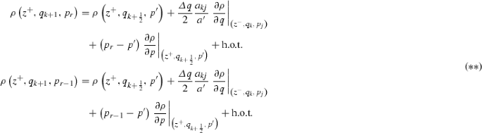
• 4. We can rewrite $(**)$ into the form

  $$\begin{aligned} \left. \frac{\partial h}{\partial \mathbf{p}} {{\mathrm{\scriptstyle \mathop {{}}\limits ^{\bullet }}}}\frac{\partial \rho }{\partial \mathbf{q}} \right| _{ -} - \left. \frac{\partial h}{\partial \mathbf{q}} \right| _- {{\mathrm{\scriptstyle \mathop {{}}\limits ^{\bullet }}}}\left( \left. \frac{\partial {\varvec{{\mathcal {S}}}}}{\partial \mathbf{p}} \right| _{\mathbf{p}^-}^{\mathrm {T}} \left. \frac{\partial \rho }{\partial \mathbf{p}} \right| _+ \right) = \left. \frac{\partial h}{\partial \mathbf{p}} {{\mathrm{\scriptstyle \mathop {{}}\limits ^{\bullet }}}}\frac{\partial \rho }{\partial \mathbf{q}} \right| _+ - \left. \frac{\partial h}{\partial \mathbf{q}} {{\mathrm{\scriptstyle \mathop {{}}\limits ^{\bullet }}}}\frac{\partial \rho }{\partial \mathbf{p}} \right| _+, \end{aligned}$$

  where applying (14) gives (13).

$\square$

Fig. 3

Evolution of the second characteristic with distances indicated. The base characteristic $(\mathbf{q}_1,\mathbf{p}_1)$ is indicated with a bullet, $(\mathbf{q}_2,\mathbf{p}_2)$ is indicated with a square and $(\mathbf{q}_3,\mathbf{p}_3)$ is indicated with a triangle

Remark

Using the definition of the Poisson bracket,

$$\begin{aligned} \left\{ f, g \right\} := \frac{\partial f}{\partial \mathbf{q}} {{\mathrm{\scriptstyle \mathop {{}}\limits ^{\bullet }}}}\frac{\partial g}{\partial \mathbf{p}} - \frac{\partial f}{\partial \mathbf{p}} {{\mathrm{\scriptstyle \mathop {{}}\limits ^{\bullet }}}}\frac{\partial g}{\partial \mathbf{q}}, \end{aligned}$$

(15)

we can rewrite the jump condition (13) into a very concise form,

$$\begin{aligned} \left\{ \rho , h \right\} _- = \left\{ \rho ,h \right\} _+. \end{aligned}$$

(16)

Corollary 2

When the interface is curved, we must adjust the result of Theorem 2 as follows,

$$\begin{aligned} \left. \left[ \frac{\partial \rho }{\partial \mathbf{q}} {{\mathrm{\scriptstyle \mathop {{}}\limits ^{\bullet }}}}\left( \frac{\partial h}{\partial \mathbf{p}} - {\mathbf {Q}}^\prime \left( z^\star \right) \right) - \frac{\partial h}{\partial \mathbf{q}} {{\mathrm{\scriptstyle \mathop {{}}\limits ^{\bullet }}}}\frac{\partial \rho }{\partial \mathbf{p}} \right] \right| _{-} = \left. \left[ \frac{\partial \rho }{\partial \mathbf{q}} {{\mathrm{\scriptstyle \mathop {{}}\limits ^{\bullet }}}}\left( \frac{\partial h}{\partial \mathbf{p}} - {\mathbf {Q}}^\prime \left( z^\star \right) \right) - \frac{\partial h}{\partial \mathbf{q}} {{\mathrm{\scriptstyle \mathop {{}}\limits ^{\bullet }}}}\frac{\partial \rho }{\partial \mathbf{p}} \right] \right| _{+}, \end{aligned}$$

(17)

where ${\mathbf {Q}} : {\mathbb {R}}^+ \rightarrow {\mathcal {Q}}$ differentiable and ${\mathbf {Q}}(z^\star )$ gives the intersection point of a characteristic with the surface. Furthermore, (14) is also valid.

Proof

A curved interface is represented by a plane in phase space moving with velocity ${\mathbf {Q}}^\prime (z)$. Hence, we perform a coordinate transform affecting the ${\mathbf {q}}$-direction only, defined as

$$\begin{aligned} \tilde{{\mathbf {q}}} = {\mathbf {q}} - {\mathbf {Q}}(z), \end{aligned}$$

which results in a coordinate system where the surface is standing still. Thus, in the new coordinate system, the surface is flat and we can apply Theorem 2. To finish, we note that Theorem 2 can be read as

Hence, we obtain that we must apply $(*)$ to $\rho (z, {\mathbf {q}}(z) - {\mathbf {Q}}(z) , {\mathbf {p}}(z))$, yielding (17). $\square$

Remark

We may alternatively view the coordinate transform as a canonical transformation, with the new Hamiltonian given by

$$\begin{aligned} \tilde{h}(z,{\mathbf {q}},{\mathbf {p}}) = h(z,{\mathbf {q}},{\mathbf {p}}) - {\mathbf {Q}}^\prime (z) {{\mathrm{\scriptstyle \mathop {{}}\limits ^{\bullet }}}}{\mathbf {p}}. \end{aligned}$$

(18)

It is important to note that Theorem 2 is true in a very general setting. Its formulation is independent of the particular form of the Hamiltonian or the coordinate system. It is therefore true in mechanics as well as optics, it is even valid independent of the evolution coordinate. We can, for instance, find a Hamiltonian system describing geometrical optics in terms of real time or arc length.

The jump condition (13) is a consequence of the transformation on phase space from $z^-$ to $z^+$ being symplectic [36]. From (11), we see that $\rho$ is constant along the characteristics. Therefore, if the influence of an interface is to move characteristics closer to each other in the $\mathbf{q}$-direction, they must get further apart in the $\mathbf{p}$-direction, which is reflected in the gradient of $\rho$ through Theorem 2.

6 Derivation of the Scheme

In this section, we aim to develop a scheme to solve Liouville’s equation numerically. The setting is two-dimensional to avoid large and cumbersome expressions. The numerical scheme for higher-dimensional systems is indeed very similar. Note that the position q and momentum p are now scalar quantities. We define the advection speeds on the screen, given by

$$\begin{aligned} a(z,q,p)&:= \frac{\partial h}{\partial p} = \frac{p}{\sqrt{n(z,q)^2-p^2}} , \end{aligned}$$

(19a)

$$\begin{aligned} b(z,q,p)&:= - \frac{\partial h}{\partial q} = \frac{n(z,q)}{\sqrt{n(z,q)^2-p^2}} \frac{\partial n}{\partial q}. \end{aligned}$$

(19b)

We look for approximate solutions to

$$\begin{aligned} \frac{\partial \rho }{\partial z} + a \, \frac{\partial \rho }{\partial q} + b \frac{\partial \rho }{\partial p} = 0, \end{aligned}$$

(20)

under the additional condition that whenever n changes discontinuously, we have

$$\begin{aligned} \rho \left( z^-, q^- , p^- \right) = \rho \left( z,^+, q^+ , p^+ \right) , \end{aligned}$$

(21)

with $p^-$ and $p^+$ related through Snell’s law and $q^- = q^+$, $z^-=z^+$. For completeness, we quote Snell’s law in two-dimensional form. Note that $\nu \in {\mathbb {R}}$ such that $| \nu | \le 1$, and we have

$$\begin{aligned} {\mathcal {S}} \left( p;n_1,n_2,\nu \right) := {\left\{ \begin{array}{ll} p - \left( \psi + {{\mathrm{sgn}}}\left( n_2 \right) \sqrt{\delta } \, \right) \nu &{} \text { if } \delta \ge 0,\\ p - 2 \psi \nu &{} \text { if } \delta < 0, \end{array}\right. } \end{aligned}$$

(22a)

where

$$\begin{aligned} \delta := n_2^2 - n_1^2 + \psi ^2 \quad \text { and } \quad \psi := p\nu \pm \sqrt{n_1^2 - p^2}\sqrt{1 - \nu ^2} , \end{aligned}$$

(22b)

where the sign is to be taken such that $\psi \le 0$, which follows from the angle convention of Snell’s law.

We apply a grid on phase space such that we have $\left\{ q_i\right\} _{i=1}^{N}$ for the positions and $\left\{ p_j \right\} _{j=1}^{M}$ for the momenta. We rescale the position space such that we have $q \in [0,1]$, giving

$$\begin{aligned} q_i := (i-1) \varDelta q, \quad \varDelta q := \frac{1}{N -1}, \end{aligned}$$

(23)

where $i \in \left\{ 1,\ldots ,N \right\}$. Note that the advection speeds, a and b, go to infinity for p close to n(q, z). Therefore, in many cases it is practical to choose a maximum allowed momentum in the system, $p_\text {max}$. This corresponds roughly to setting a maximum angular aperture. The discretization of p is thus defined as

$$\begin{aligned} p_j := \tfrac{1}{2}(2j-M-1)\varDelta p,\quad \varDelta p :=2 \frac{ p_\text {max}}{M-1}, \end{aligned}$$

(24)

for $j = \{1,\ldots ,M \}$. Finally, we discretize z as

$$\begin{aligned} z^t := (t-1) \varDelta z , \quad \varDelta z = \frac{z_\text {max}}{T-1}, \end{aligned}$$

(25)

for $t = \left\{ 1,\ldots ,T \right\}$ and $z_\text {max}$ is the total length of optical axis along which we integrate Liouville’s equation. The numerical approximation of the solution is then denoted by $\rho ^t_{ij} \approx \rho (z^t,q_i,p_j)$.

Let us define the positive and negative part of a number $c \in {\mathbb {R}}$ as follows,

$$\begin{aligned} c^+ := \max (c,0), \quad c^- := \min (c,0). \end{aligned}$$

(26)

Whenever the refractive index is differentiable, (20) has a classical solution and the upwind scheme is straightforwardly found as

$$\begin{aligned} \begin{aligned}&\frac{\rho ^{t+1}_{ij} - \rho ^t_{ij}}{\varDelta z} + \left( a_{ij}^t\right) ^+ \, \frac{\rho ^t_{ij}-\rho ^t_{i-1,j}}{\varDelta q} + \left( a_{ij}^t\right) ^- \, \frac{\rho ^t_{i+1,j}-\rho ^t_{ij}}{\varDelta q} \\&\quad + \left( b_{ij}^t\right) ^+ \, \frac{\rho ^t_{ij}- \rho ^t_{i,j-1} }{\varDelta p} + \left( b_{ij}^t\right) ^- \, \frac{\rho ^t_{i,j+1}- \rho ^t_{ij} }{\varDelta p} = 0, \end{aligned} \end{aligned}$$

(27)

where

$$\begin{aligned} a_{ij}^t := a\left( z^t,q_i,p_j\right) , \quad b_{ij}^t := b\left( z^t,q_i,p_j\right) . \end{aligned}$$

(28)

As one can see, the expression in a two-dimensional optical system is already quite cumbersome, though not complicated. A three-dimensional optical system will just add four more upwind difference terms.

We now wish to find a scheme that gives us the correct physical solution whenever we allow n to have discontinuities. The correction to the upwind scheme applies only locally around the interface, away from the interface the scheme will be given by (27). Thus, to illustrate our method, we use the simplest case of a piecewise constant refractive index. We choose a system that has $0 \le q \le 1$, fix $1 < k < N$, and let us place the interface at $q_{k+\frac{1}{2}} = q_k + \frac{1}{2} \varDelta q$, thus we have

$$\begin{aligned} n(q) = {\left\{ \begin{array}{ll} n_1 &{} \text { if } q < q_{k+\frac{1}{2}},\\ n_2 &{} \text { if } q \ge q_{k+\frac{1}{2}}. \end{array}\right. } \end{aligned}$$

(29)

It is clear that $\frac{\partial n}{\partial q} = 0$ almost everywhere, thus $b(z,q,p) =0$ at all the grid points. Away from the interface, $i \ge k+2$ or $i \le k-1$, we have a smooth refractive index, resulting in the following scheme,

$$\begin{aligned} \frac{\rho ^{t+1}_{ij} - \rho ^t_{ij}}{\varDelta z} + a_{ij}^+ \frac{\rho ^t_{ij}-\rho ^t_{i-1,j}}{\varDelta q} + a_{ij}^- \frac{\rho ^t_{i+1,j}-\rho ^t_{ij}}{\varDelta q}=0, \end{aligned}$$

(30)

where now a does not depend on z so that $a_{ij} = a(q_i,p_j)$. Even close to the interface, this scheme works as long as the upwind grid point is not on the other side of the interface. Hence,

$$\begin{aligned} \frac{\rho ^{t+1}_{kj} - \rho ^t_{kj}}{\varDelta z} + a_{kj} \frac{\rho ^t_{kj}-\rho ^t_{k-1,j}}{\varDelta q}&=0, \quad p_j \ge 0, \end{aligned}$$

(31a)

$$\begin{aligned} \frac{\rho ^{t+1}_{k+1,j} - \rho ^t_{k+1,j}}{\varDelta z} + a_{k+1,j} \frac{\rho ^t_{k+2,j}-\rho ^t_{k+1,j}}{\varDelta q}&=0,\quad p_j \le 0, \end{aligned}$$

(31b)

since the sign of $a_{ij}$ is equal to the sign of $p_j$. Let us now consider the collection of grid points $(q_k,p_j)$ with $p_j<0$ and $(q_{k+1},p_j)$ with $p_j>0$. These are grid points that have their upwind grid point on the other side of the interface. Our scheme has to be different here since the characteristics have a jump in momentum when crossing the interface. We wish to approximate $\frac{\partial \rho }{\partial q}$ at the grid point $(q_k,p_j)$, which we can do by utilizing Theorem 2.

The idea is straightforward, we make a Taylor expansion from both sides of the interface towards the interface. However, we keep Snell’s law in mind and make our expansions about the point where the characteristic is discontinuous, see Fig. 4. This allows us to approximate the gradient at $(q_k,p_j)$ using information from the other side of the interface. The resulting scheme is summarized in the following theorem.

Fig. 4

Sketch of the scheme close to the interface, the upwind grid point is on the other side of the interface. The base characteristic is indicated with arrows

Theorem 3

Consider the collection of grid points such that $\left\{ q_k , p_j<0 \right\}$. Let us denote $p^\prime = -{\mathcal {S}}(-p_j;n_2,n_1,-\nu )$, and $\delta \ge 0$ in (22a), where $\delta$ is given by (22b). The scheme is then given by

$$\begin{aligned} \frac{\rho _{kj}^{t+1}-\rho _{kj}^t}{\varDelta z} + \tilde{a} \frac{\rho ^\prime - \rho _{kj}^t}{\varDelta q} = 0, \end{aligned}$$

(32a)

where

$$\begin{aligned} \tilde{a}:= & {} 2 \left( \frac{1}{a_{kj}} + \frac{1}{a^\prime } \right) ^{-1} \quad \text {and}\quad a^\prime = \frac{p^\prime }{\sqrt{n_2^2-{p^\prime }^2}}, \end{aligned}$$

(32b)

$$\begin{aligned} \rho ^\prime= & {} \theta \rho _{k+1,r}^t + (1-\theta ) \rho _{k+1,r-1}^t, \end{aligned}$$

(32c)

where $\theta = (p^\prime - p_{r-1})/{\varDelta p}$, with r such that $p_{r-1} < p^\prime \le p_r$.

In case when, $\delta <0$, reflection occurs and we have to use (32a), now with

$$\begin{aligned} \tilde{a}:= & {} 2\left( \frac{1}{a_{kj}} - \frac{1}{a^\prime } \right) ^{-1} \quad \text {and} \quad a^\prime = \frac{p^\prime }{\sqrt{n_1^2-{p^\prime }^2}}, \end{aligned}$$

(33a)

$$\begin{aligned} \rho ^\prime= & {} \theta \rho _{k,r}^t + (1-\theta ) \rho _{k,r-1}^t. \end{aligned}$$

(33b)

Remark

The case for $\left\{ q_{k+1} , p_j >0 \right\}$ is similar.

Proof

• 1. We start by using the method of lines (MOL) approach, which is to say, we discretise space, but leave z continuous. Let us assume that j is such that $\delta \ge 0$, thus we have refraction. Let us further assume that the initial conditions are smooth. Furthermore, define $p^\prime = - {\mathcal {S}}(-p_j;n_2,n_1,-\nu )$, which we shall shorten to $p^\prime = - {\mathcal {S}}(-p_j)$, such that $p^\prime$ is the momentum that becomes $p_j$ if the characteristic traverses the interface. We define r as the unique index such that $p_{r-1} < p^\prime \le p_r$.

• 2. Performing a Taylor expansion about the relevant grid points close to the interface on the left side reveals,

  

  and similarly on the right side,

  $$\begin{aligned} \rho \big (z^+,q_{k+1},p_r\big )&= \rho \big (z^+,q_{k+\frac{1}{2}},p^\prime \big ) + \frac{\varDelta q}{2} \left. \frac{\partial \rho }{\partial q} \right| _{\big (z^+,q_{k+\frac{1}{2}},p^\prime \big )} \nonumber \\&\quad + \big (p_r-p^\prime \big ) \left. \frac{\partial \rho }{\partial p} \right| _{\big (z^+,q_{k+\frac{1}{2}},p^\prime \big )} + \text {h.o.t.}\\ \rho \big (z^+,q_{k+1},p_{r-1}\big )&= \rho \big (z^+,q_{k+\frac{1}{2}},p^\prime \big ) + \frac{\varDelta q}{2} \left. \frac{\partial \rho }{\partial q} \right| _{\big (z^+,q_{k+\frac{1}{2}},p^\prime \big )} \nonumber \\&\quad + \big (p_{r-1} - p^\prime \big ) \left. \frac{\partial \rho }{\partial p} \right| _{\big (z^+,q_{k+\frac{1}{2}},p^\prime \big )} + \text {h.o.t.} \end{aligned}$$

  where h.o.t. represents (mixed) higher order terms. Next, we perform another Taylor expansion, this time for the derivative, i.e.,

  

  Now we apply (13) to find

  $$\begin{aligned} a^\prime \left. \frac{\partial \rho }{\partial q} \right| _{\big (z^+,q_{k+\frac{1}{2}},p^\prime \big )} = a_{kj} \left. \frac{\partial \rho }{\partial q} \right| _{\big (z^-,q_{k+\frac{1}{2}},p_j\big )}, \end{aligned}$$

  where $a^\prime$ is given by (32b 32c). Hence, combining this with $(\#)$ gives us

  $$\begin{aligned} \left. \frac{\partial \rho }{\partial q} \right| _{\big (z^+,q_{k+\frac{1}{2}},p^\prime \big )} = \frac{a_{kj}}{a^\prime } \left. \frac{\partial \rho }{\partial q} \right| _{\big (z^-,q_{k},p_j\big )} + {\mathcal {O}}(\varDelta q), \end{aligned}$$

  and consequently

  

  where again, h.o.t represents mixed higher order terms.

• 3. We will now take a linear combination of the values of $\rho$ at the three grid points given by $(*)$ and $(**)$. We wish to find a linear combination which approximates the q-derivative of $\rho$ at the grid point $(q_k,p_j)$. Assume that $\lambda _l \in {\mathbb {R}}$, for $l = 1,2,3$, then the upwind finite difference should satisfy

  $$\begin{aligned} \left. \frac{\partial \rho }{\partial q} \right| _{\left( z^-,q_k,p_j\right) } \approx \lambda _1 \rho \left( z^-,q_k,p_j\right) + \lambda _2 \rho \left( z^+,q_{k+1},p_r\right) + \lambda _3 \rho \left( z^+,q_{k+1},p_{r-1}\right) , \end{aligned}$$

  where the approximation should be correct up to first-order. Using (21), we find the following system of equations,

  $$\begin{aligned} \lambda _1 + \lambda _2 + \lambda _3 = 0, \\ \frac{\varDelta q}{2} \left( \frac{a_{kj}}{a^\prime } \lambda _2 + \frac{a_{kj}}{a^\prime } \lambda _3 -\lambda _1 \right) = 1, \\ \lambda _2 \left( p_r - p^\prime \right) + \lambda _3 \left( p_{r-1} - p^\prime \right) = 0, \end{aligned}$$

  where one should note that the determinant of this linear system is non-zero. Defining $\tilde{a}$ as the harmonic mean of $a_{kj}$ and $a^\prime$, see (32b 32c), we find the solution of this system as

  $$\begin{aligned} \lambda _1 = - \frac{\tilde{a}}{a_{kj}} \frac{1}{\varDelta q}, \quad \lambda _2 = \frac{\tilde{a}}{a_{kj}} \frac{\theta }{\varDelta q}, \quad \lambda _3 = \frac{\tilde{a}}{a_{kj}} \frac{1-\theta }{\varDelta q}, \end{aligned}$$

  where $\theta = (p^\prime - p_{r-1})/{\varDelta p}$. We now approximate $\left. \frac{\partial \rho }{\partial z}\right| _{(z^t,q_k,p_j)} \approx \frac{\rho ^{t+1}_{kj} - \rho ^t_{kj}}{\varDelta z}$, whence we find the scheme

  $$\begin{aligned} \frac{\rho ^{t+1}_{kj} - \rho ^t_{kj}}{\varDelta z} + \tilde{a} \frac{\theta \rho _{k+1,r}^t + (1-\theta )\rho _{k+1,r-1}^t - \rho _{kj}^t }{\varDelta q} =0. \end{aligned}$$

  Recognizing that $\rho ^\prime := \theta \rho _{k+1,r}^t + (1-\theta )\rho _{k+1,r-1}^t$ is nothing but a linear interpolation approximating $\rho (z^t,q_{k+1},p^\prime )$, we find (32a).

• 4. When j is such that $\delta < 0$, we have reflection and the derivation is largely the same. The only difference being that the upwind grid points are now given by $(q_k,p_r)$ and $(q_k,p_{r-1})$ instead of $(q_{k+1},p_r)$ and $(q_{k+1},p_{r-1})$. After doing completely similar operations, we find (32a) but now with $\rho ^\prime$ given by (33b) and $a^\prime$ given by (33a).

$\square$

Remark

When the surface is curved we find that we must furthermore replace $a_{kj}$ with $a_{kj} - Q^\prime (z^\star )$ and $a^\prime$ with $a^\prime - Q^\prime (z^\star )$.

The correction for the advection speed enforces that the mapping from $z^-$ to $z^+$ is symplectic. In going from a high refractive index to a lower one, the transmitted light is stretched in the p-direction. The slightly higher advection speed near the interface can be interpreted as a shrinking of the q-direction, thereby preserving area in phase space.

From Theorem 3, we see that the scheme close to an interface is still an upwind scheme and in fact, (32a) has completely the same form as (30). However, we must replace both the advection speed and the value of $\rho$ at the upwind grid point. Fortunately, the replacement values can be explicitly computed by invoking Snell’s law. The scheme is in essence a first order accurate upwind scheme, with the correction only occurring near the interface. We thus expect the scheme to be globally first order accurate.

When considering variable refractive index fields together with interfaces, we can again employ Theorem 3. However, away from the interface we must now use (27) and only correct the terms approximating $\frac{\partial \rho }{\partial q}$. The interface position does not depend on p and therefore the flow across an interface may only be driven by $\frac{\partial h}{\partial p}$. Thus, the flow across an interface cannot depend on the gradient of the refractive index field, provided we use a standard Cartesian discretisation. It is for this reason that we shall not consider variable index fields in the following.

6.1 Implementation of Curved Interfaces

Most optical systems have a curved interface, like any lens or focussing mirror, and consequently do not have an axis along which the refractive index field is constant. Thus, as we move along the optical axis, the refractive index field will change. The interfaces will therefore also move, in position space ${\mathcal {Q}}$, as a function of z. Let us assume that we can describe the position of the interface with a differentiable function $Q: {\mathbb {R}}^+ \rightarrow {\mathbb {R}}^d$. Then the position of the interface defines a moving plane in phase space, or line in the two-dimensional case.

In such a case, it might occur that at one z-level, the surface is on one side of a column of grid points and at the next it is on the other side. Thus, fix some $l \in \{1,\ldots ,N\}$ and consider the maximum z-level $\tau$ such that $q_l \le Q(z^\tau ) < q_{l+1}$. Then, by definition, we have that $Q(z^{\tau +1}) \ge q_{l+1}$ and it may happen that $\rho ^{\tau +1}_{l+1,m} = 0$ for all $m = \{1,\ldots ,M\}$, see Fig. 5a. This situation is especially likely to happen whenever the surface is a reflector.

Fig. 5

A z-step causes the interface (dashed line) to cross a column of grid points. The base characteristics are indicated with a dotted line

The situation described is of course non-physical and completely due to the discretisation of phase space. However, we can correct the resulting error by interpolation across base characteristics. Hence, we keep track of when the interface moves across a column of grid points and check whether the solution needs correction. If it does need correction, we perform an interpolation across the base characteristics. Let us fix j and assume that some base characteristic undergoes a momentum change from $p_j$ to $p^\prime$ and $p_{r-1} < p^\prime \le p_r$. Then we have, possibly, that $\rho ^{\tau +1}_{l,r-1} \ne 0$, $\rho ^{\tau +1}_{l,r} \ne 0$ and $\rho ^{\tau +1}_{l,j} \ne 0$. We interpolate between these three points to correct $\rho ^{\tau +1}_{l+1,j}$. In this way, whenever the solution is zero somewhere due to an artefact of the discretisation, we may correct it. After the interpolation in the p-direction to obtain values for $\rho$ on $q_l$ and $p^\prime$, we have essentially a one-dimensional case across the base characteristic.

Thus, we first find $p^\prime =-{\mathcal {S}}(-p_j;n_2,n_1,-\nu )$, where $n_1 = n_2$ in case of reflection. Next, we find r such that $p_{r-1} < p^\prime \le p_r$ and we compute $\theta = \frac{p^\prime - p_{r-1}}{\varDelta p}$. We then define $\rho ^\prime = \theta \rho _{lr}^{\tau +1} + (1-\theta ) \rho _{l,r-1}^{\tau +1}$. This gives us a value on the base characteristic at $p^\prime$ and $q_l$. This value is then used to interpolate across the base characteristic connecting $\rho _{lj}^{\tau +1}$ and $\rho ^\prime$, the total distance between these two points is $2(\varDelta q + \varDelta q^\prime )$, where $\varDelta q^\prime =Q(z^{\tau +1}) - q_{l+1}$. Let us write

$$\begin{aligned} \mu = \frac{\varDelta q}{2\left( \varDelta q + \varDelta q^\prime \right) }, \end{aligned}$$

(34)

so that we obtain the corrected value $\tilde{\rho }_{l+1,j}^{\tau +1}$ as

$$\begin{aligned} \tilde{\rho }_{l+1,j}^{\tau +1} = \left( 1 - \mu \right) \rho _{lj}^{\tau +1} + \mu \rho ^\prime . \end{aligned}$$

(35)

7 Results

As argued previously, a continuously varying refractive index will not influence the scheme near the interface in a substantial way. Thus, for the sake of simplicity, we present two cases which will exhibit all the features of the scheme that are different from a standard first-order upwind scheme. The first is the Bucket of Water problem, introduced in Sect. 4, which can be solved analytically fairly easily. The second test case is the two-dimensional Compound Parabolic Concentrator (CPC).

In the second test case, the CPC, we shall compare our method with Monte Carlo ray tracing, see for instance [43]. This procedure involves choosing a number of rays with randomized initial conditions, tracing their trajectory through the optic and subsequently performing a box count. The box count is often necessary because a proper interpolation is too complicated. Thus, to make a comparison between ray tracing and our method, we should pick a representative number of rays per grid point, the control volume of each grid point forming a box in phase space. The average number of rays per box can be quite high, depending on the desired accuracy. In practice, 100 rays per box is a typical number.

7.1 Bucket of Water

We take a simple jump in refractive index as in (29) and we pick $n_1=1.4$ and $n_2=1$. The refractive index field is given by

$$\begin{aligned} n(q) := {\left\{ \begin{array}{ll} n_1 &{} \text {if } q\le q_{k+\frac{1}{2}},\\ n_2 &{} \text {if } q > q_{k+\frac{1}{2}}, \end{array}\right. } \end{aligned}$$

(36)

where we pick k such that $q_{k+\frac{1}{2}} = \frac{1}{2} + {\mathcal {O}}(\varDelta q)$. This case corresponds roughly to a water-air transition, and we shall at times refer to this problem as the Bucket of Water problem. One important thing to note is that the optical axis is parallel to the interface, resulting in a refractive index field which does not depend on z, see Fig. 6.

Fig. 6

Bucket of Water problem: the hatchings indicate a domain of different refractive index. Note that the optical axis is parallel to the refractive surface

The reason we choose this particular problem is because it exhibits both refraction and TIR. At the same time, the problem is solvable by the method of characteristics, see Appendix 2 for a complete description. The exact solution is given by

$$\begin{aligned} \rho (z,q,p) = {\left\{ \begin{array}{ll} \rho _0\left( q - z a(n_1,p), p \right) , &{} \text { if } q < \frac{1}{2}, p \ge 0\\ \rho _0 \left( 1 - q - z a(n_1,-p) , -p \right) , &{} \text { if } q < \frac{1}{2}, -p_c < p <0, \\ \rho _0 \left( \frac{1}{2} - \left( z - \varDelta z(q,p)\right) a\left( n_2,p^\prime \right) ,p^\prime \right) , &{} \text { if } q \ge \frac{1}{2}, p \ge 0, \\ 0 &{} \text { otherwise}, \end{array}\right. } \end{aligned}$$

(37)

where $p^\prime = -{\mathcal {S}}(-p;n_2,n_1,-\nu )$ with ${\mathcal {S}}$ defined in (22a). In (37), the first statement is free propagation, the second is refraction, the third comes from total internal reflection and the fourth statement comes from the compact support of $\rho _0$. We introduce the critical momentum $p_c = \sqrt{n_1^2 - n_2^2} = 0.9798$, where with $p<p_c$ total internal reflection occurs. This condition is perhaps counter-intuitive, however this is due to the choice of optical axis. We furthermore define the following quantity,

$$\begin{aligned} \varDelta z (q,p) :=\frac{\frac{1}{2} - q}{p} \sqrt{n_2^2 - p^2}. \end{aligned}$$

(38)

A ray which passes through the point (q, p) at z will hit the interface at $z-\varDelta z(q,p)$. The variable a is simply the propagation speed on the screen. We see that, although in principle not too difficult to solve, the expressions become large and unwieldy. Going to a slightly more complicated geometry already precludes the solvability by hand.

We take as initial condition the distribution

$$\begin{aligned} \rho _0(q,p) = {\left\{ \begin{array}{ll} 1 &{} \text { if } 0.3 \le q \le 0.35 \text { and } 0 \le p \le 1.1, \\ 0 &{} \text { otherwise}, \end{array}\right. } \end{aligned}$$

(39)

see Fig. 7. These initial conditions contain the critical momentum $p_c$, such that both refraction and total internal reflection will occur. The exact solution to the Bucket of Water problem is plotted in Fig. 8.

Fig. 7

Initial condition of the Bucket of Water problem, black has value 1 and white has value 0. The transition is at $q = \frac{1}{2}$ and indicated with a dashed line. The line $p = 0$ is also indicated with a dashed line

We use an integration length of $z = 0.4$ with 1000 steps on an $800 \times 800$ grid. For the discretization of phase space we use 800 grid points for both position and momentum, see Fig. 9. We see from Fig. 8 and 9 that the numerical solution is very close to the exact solution. The only difference that is noticeable by eye is the numerical diffusion at the edges. However, note that the edge at the interface is sharp. The numerical diffusion is of course an effect of the first order accurate upwind scheme. The sharp edges are an effect of the discrete symplectic transformation which occurs at the interface. In fact, the scheme is entirely symplectic in principle, the diffusion is generated by the linear interpolation that is inherent in the upwind scheme.

Fig. 8

Exact solution to the Bucket of Water problem at $z=0.4$

Fig. 9

Numerical solution to the Bucket of Water problem $z=0.4$

In this case, the Bucket of Water problem, we can implement the scheme in a matrix-vector formulation, where the evolution matrix is fixed. Hence, we only have to compute this evolution matrix once, and we can then use it for any initial condition. Every step in z then becomes a matrix-vector product, where the matrix is very sparse. This will not be the case in our next example, where the evolution matrix has to be recomputed every time step. However, we shall first investigate numerically the convergence properties of the scheme.

7.1.1 Convergence Results

The convergence of our scheme is tested numerically by performing several runs of the Bucket of Water problem with different grid sizes. The refractive index is once again given by (36). However, as our analysis of the error is only valid for functions that are smooth away from the interface, we will use a smooth initial condition, $\rho _0 \in C^\infty _0({\mathcal {P}})$. This initial condition is constructed by using the “bump” function [44], given by

$$\begin{aligned} \psi (x) := {\left\{ \begin{array}{ll} e^{-\frac{1}{1-x^2}}, &{} \text {for } |x|<1,\\ 0, &{} \text {otherwise}. \end{array}\right. } \end{aligned}$$

(40)

One can check that the bump function is infinitely smooth and has compact support. The initial condition is constructed as follows,

$$\begin{aligned} \rho _0 (q,p) := \psi \left( \frac{q-q_0}{\lambda _q} \right) \psi \left( \frac{p-p_0}{\lambda _p} \right) , \end{aligned}$$

(41)

where

$$\begin{aligned} q_0 = \tfrac{1}{4}, \quad \lambda _q = \tfrac{3}{20}, \quad p_0 = \tfrac{3}{5}, \quad \lambda _p = \tfrac{1}{2}, \end{aligned}$$

(42)

which results in the support of $\rho _0$ being $\left\{ \tfrac{1}{10} \le q \le \tfrac{2}{5} , \tfrac{1}{10} \le p \le \tfrac{11}{10} \right\}$. The integration time is chosen as $z = \tfrac{2}{5}$, which results in a large part of the initial condition to be refracted and reflected by the interface.

We compute the error by using the exact solution and taking the $L^1$-norm of the difference, i.e.,

$$\begin{aligned} {\mathrm {e}}_L = \sum \limits _{i=1}^N \sum \limits _{j=1}^M \left| \rho ^T_{ij} - \rho \left( q_i,p_j,z^T \right) \right| \varDelta q \varDelta p, \end{aligned}$$

(43)

where $z^T = \tfrac{2}{5}$. For simplicity, we shall choose $\varDelta q = \varDelta p$, the results are displayed in Table 1.

Table 1 Error and convergence rates using the Bucket of Water Problem as a benchmark

As the analytical solution for this problem is known, we can use it as a benchmark test and determine the error of our solver exactly. The results clearly show that our scheme is first order accurate in the number of grid points in the q-direction. This is as expected since an ordinary upwind solver has an error of ${\mathcal {O}}(\varDelta q)+{\mathcal {O}}(\varDelta p)$. The adjustments to the upwind scheme have virtually no impact on the error behaviour.

7.2 Compound Parabolic Concentrator

The compound parabolic concentrator (CPC) is a pair of mirrors that have a parabolic shape. The CPC represents a worst-case scenario for Liouville’s equation, as many different parts of phase space are interacting. Furthermore, the curved mirrors force us to recompute the evolution matrix at each time step. There are rays present that travel perpendicular to the optical axis that have a significant influence on the output, which causes a severe time-step restriction. These issues are not present when one uses a ray tracing method. Moreover, the CPC allows analytical computation of the intersection point of a ray with the mirrors. Thus, the CPC presents many issues for our scheme while presenting many advantages to ray tracing methods.

We assume that the CPC is embedded in a medium of unit refractive index, say air. In two dimensions, the CPC has ideal transmission characteristics, meaning all incoming light within an acceptance angle $\theta$ at the entrance aperture is captured and concentrated onto the exit aperture [45]. The exit aperture is represented by the subset $(-a,a) \times (-1, 1) \subset {\mathcal {P}}$. The CPC can be constructed by tilting two parabolas, one over angle $\theta$ and one over angle $-\theta$, and shifting them such that their focal points are at $(-a,0)$ and (a, 0), respectively. Finally, one has to pick the focal point distance such that the parabolae go through the points (a, 0) and $(-a,0)$, respectively, see Fig. 10.

Fig. 10

The CPC is constructed by tilting and shifting two parabolas

After rotating and shifting a standard parabola and setting the focal point correctly, one wall of the CPC can be characterized by the equation,

$$\begin{aligned}&\left( q \cos \theta + z \sin \theta \right) ^2 + a \left( 1 + \sin \theta \right) ^2 q - a \cos \theta \left( 2 + \sin \theta \right) ^2 z \nonumber \\&\quad - \frac{a^2}{4} \left( 1 + \sin \theta \right) \left( 3 + \sin \theta \right) = 0. \end{aligned}$$

(44)

We can solve (44) for q and select the positive root, which we define as $Q_r:{\mathbb {R}}^+ \rightarrow {\mathbb {R}}$. For positive q, we use $q = Q_r(z)$ as the curve defining the wall of the CPC, for negative q we use $-q = Q_r(z)$. The normal can be found easily, since $Q_r$ is differentiable. The shape of a CPC with exit aperture 2a and acceptance angle $\theta$ is completely fixed. The optic has a length Z, given by

$$\begin{aligned} Z = a\frac{(1+\sin \theta )\cos \theta }{\sin ^2 \theta }, \end{aligned}$$

(45)

while the half-width of the entrance aperture is given by

$$\begin{aligned} a^\prime = \frac{a}{\sin \theta }. \end{aligned}$$

(46)

We can apply Liouville’s Theorem to find how area in phase space is transformed when traversing the CPC. The CPC accepts momenta in the range $(-\sin \theta , \sin \theta )$, while the spatial aperture is given by (46), thus the total area in phase space representing the entrance aperture is 4a. The exit aperture has width 2a, so the range of momenta at the exit aperture must be $(-1,1)$, which corresponds to an angular range of $(-\tfrac{\pi }{2},\tfrac{\pi }{2})$. Hence, the CPC provides maximal concentration in the spatial coordinate, while the price to pay is maximum dilution in the angular coordinate.

This also provides us with a special case that allows us to construct an exact solution to Liouville’s equation. If the solution is given by the characteristic function of $(-a^\prime ,a^\prime ) \times (-\sin \theta , \sin \theta )$ at the entrance aperture, the solution at the exit aperture must be the characteristic function of $(-a,a)\times (-1,1)$. Conversely, using as an initial condition

$$\begin{aligned} \rho _0(q,p) = {\left\{ \begin{array}{ll} 1, &{} \text {for } -a \le q \le a, -1 \le p \le 1,\\ 0, &{} \text {otherwise}, \end{array}\right. } \end{aligned}$$

(47)

the solution at $z = Z$ is then given by

$$\begin{aligned} \rho (Z,q,p) = {\left\{ \begin{array}{ll} 1, &{} \text {for } -a \le q \sin \theta \le a, -\sin \theta \le p \le \sin \theta ,\\ 0, &{} \text {otherwise}. \end{array}\right. } \end{aligned}$$

(48)

The results are plotted in Figs. 11 and 12. We compute the numerical solution using a $300 \times 300$ grid and 500 time steps. We have used $\theta = \frac{\pi }{6}$ and $a = \frac{1}{2}$. We have integrated Liouville’s equation on the CPC to $z= Z$ given by (45).

Fig. 11

Exact solution for the CPC

Fig. 12

Numerical solution for the CPC

Fig. 13

Intermediate result at $z = Z/3$

The figure shows a great resemblance between the numerical and exact solutions. Besides from some numerical diffusion at the top and bottom edges, the numerical solution is equal to the exact solution. An intermediate result at $z = Z/3$ is shown in Fig. 13. It shows that the numerical diffusion comes from the upwind scheme, whereas the sharp edges come from the symplectic transformation that is the reflection.

We shall now compare our scheme to Monte Carlo ray tracing, which is used in conjunction with a scaled histogram to represent the solution. The histogram is scaled with the average number of rays per grid point such that the average value of the scaled histogram is equal to unity. By the Central Limit Theorem, we see that this procedure converges with the square root of the average number of rays per box, i.e., $e_{{\mathrm {RT}}} \sim \sqrt{\frac{M}{N_{{\mathrm {RT}}}}}$, where M is the number of boxes. In our comparison, we use the control volume of a grid point as the box, with $N_p = N_q$ leading to $N_q^2$ boxes and thus $e_{{\mathrm {RT}}} \sim \frac{N_q}{\sqrt{N_{{\mathrm {RT}}}}}$. However, it is important to note that even when $N_{{\mathrm {RT}}} \rightarrow \infty$, we are essentially making a piecewise constant approximation to the solution and therefore a first-order error in the box size. Thus, for Monte Carlo ray tracing, the total error scales as

$$\begin{aligned} e_{{\mathrm {RT}}} = {\mathcal {O}}\left( \frac{N_q}{\sqrt{N_{{\mathrm {RT}}}}} \right) + {\mathcal {O}}\left( \frac{1}{N_q} \right) . \end{aligned}$$

(49)

It can be shown that the minimum error is made for $N_{{\mathrm {RT}}} \sim N_q^4$.

The Liouville solver is again implemented using a matrix-vector formulation. We first construct a basic evolution matrix, where every time step needs only $2N_q$ elements adjusted from the basic evolution matrix. The exact solution is only known at $z=Z$, hence that is where we compare both methods against the exact solution. We choose $N_p = N_q$ and we fix the CFL number for the q-direction to be 0.96. Note that for a given initial position of a ray one can analytically determine the intersection points with the CPC. Thus, this test case is certainly favouring the ray tracing method, as more general optics would require a root finding method to find all intersection points, adding to the computation time. Ray tracers may also generate errors by not finding the right intersection point.

Next, we will vary the number of grid points, and therefore the boxes, but we keep the average number of rays per box constant. We point out that typical choices for the grid size in applications are $300 \times 300$, hence we have chosen our comparison to include this particular value. We have fixed the average number of rays per grid point at 100, thus choosing $N_{{\mathrm {RT}}} = 100 N_q^2$, the results are displayed in Table 2.

Table 2 Computation times and error of the CPC test case, $\tilde{t}_{{\mathrm {RT}}}$ are extrapolated times such that the error due to ray tracing is equal to the corresponding case of our scheme

For all grid sizes, our method is faster, in terms of computation time, than Monte Carlo ray tracing. One does notice that the scaling behaviour is different, ray tracing having a linear time scaling behaviour in the number of rays, $t_{{\mathrm {RT}}}\sim N_{{\mathrm {RT}}}$ and our method having quadratic time scaling in the total number of grid points $t_L\sim (N_q N_p)^2$, which in our case reduces to $t_L \sim N_q^4$. However, this is the same scaling as we have found earlier to produce a minimal error for the ray tracer.

Let us fix $N_q$ and assume ${\mathrm {e}}_{{\mathrm {RT}}} \sim \frac{1}{\sqrt{N_{{\mathrm {RT}}}}}$, thus ignoring the error due to the box count. Again, the ray tracer takes a computation time of $t_{{\mathrm {RT}}} \sim N_{{\mathrm {RT}}}$, allowing an estimate of the computation time to achieve the desired error tolerance. Suppose we want to reduce the error by a factor of c, then we have to increase the number of rays by a factor of $\frac{1}{c^2}$. Consider the case $N_{{\mathrm {RT}}}= 10^6$ from Table 2, and let us estimate the necessary number of rays to obtain the same global error as by solving Liouville’s equation with $N_q = 100$. We find the scaling constant as $c=\frac{8.31 \cdot 10^{-2}}{0.1394} = 0.5961$ and $\frac{1}{c} = 1.6775$ leading to $2.8 \cdot 10^6$ rays needed. The time would then also multiply by a factor of $\frac{1}{c^2}$, leading to a computation time of 1 min 50 s. Rescaling the other computation times to obtain the same error as the corresponding Liouville solver cases leads to estimated times of 11 min 47 s, 33 min 9 s and 1 h 9 min 55 s respectively. These estimated times are also presented in Table 2 as $\tilde{t}_{{\mathrm {RT}}}$. Note, however, that the assumption of a negligible error due to the box count results in these estimates being lower bounds.

The fact that these estimates are lower bounds can be demonstrated by numerically investigating the convergence behaviour of the Monte Carlo ray tracing method. We shall fix $N_q = 100$ and run the ray tracer for 1,4,9 and 16 million rays, the results are displayed in Table 3. The table clearly shows that only for 16 million rays is the ray tracing method really approaching the same global error as our scheme. Since the computation time for ray tracing only depends on the number of rays, we may read the computation times from Table 2. Thus, in reality, using ray tracing to obtain a solution that has the same global error as our scheme will take a much longer time than the estimates from Table 2.

Table 3 Errors for the Monte Carlo ray tracing method with a fixed number of $100 \times 100$ boxes

Hence, solving Liouville’s equation appears to be much more efficient in terms of computing time when a specific error tolerance has to be met. We conclude that when one is interested in obtaining the full phase space description, solving Liouville’s equation is certainly a more efficient approach compared to Monte Carlo ray tracing. There are increasingly many applications where full information on phase space is desirable, e.g., the optical mixing of light and the studying of aberrations in free-form optics [9, 10].

8 Conclusions

We have constructed a numerical method which is able to obtain the correct physical solution to Liouville’s equation when the Hamiltonian is discontinuous. We have done this by building the correct physics into the numerical scheme. When there are no interfaces, i.e., discontinuities in the Hamiltonian, the scheme is simply the upwind scheme. When encountering an interface, the upwind grid point is selected using Snell’s law.

Furthermore, we have derived a general jump condition assuming the initial conditions are smooth. This jump condition is what allowed us to derive a consistent scheme. In the case of a simple jump such as the Bucket of Water, the resulting advection speed is the harmonic average of the speeds on both sides of the interface.

For very simple geometries, we can apply the method of characteristics (MOC) to find a global solution analytically. We find excellent agreement between the exact and numerical solutions. The only difference being the numerical diffusion that is inherent in first order methods for hyperbolic PDEs. We were also able to apply our scheme to the compound parabolic concentrator (CPC) with great success. Liouville’s equation has no global analytical solution for the CPC. However, in an important special case, we can find the solution at the entrance and exit apertures, based on Liouville’s Theorem. Apart from some numerical diffusion around $p = \pm \sin \theta$, where $\theta$ is the acceptance angle, the numerical solution is equal to the exact solution. We have also shown by these two examples that our solver for Liouville’s equation gives an approach that is likely to be more efficient, in terms of computation time, than Monte Carlo ray tracing. Especially when a certain error tolerance is to be met, our approach is certainly faster.

We intend to extend our scheme to a three-dimensional optical setting. A naive approach of a uniform grid quickly grows to be computationally infeasible. Whereas phase space in a two-dimensional optical setting is two-dimensional, for a three-dimensional setting phase space becomes four-dimensional. Hence, a uniform grid will have $N^4$ grid points as opposed to the $N^2$ in the two-dimensional case. Our research effort will therefore be focused on non-uniform grids and hopefully we may drastically reduce the number of grid points needed.

In future work, we might also extend our scheme to include the Fresnel coefficients at sharp interfaces. When Fresnel reflection is taken into account, we must adjust (5) accordingly. Fresnel’s equations specify exactly how much light is reflected and transmitted and thus, we will be able to find a numerical solution to Liouville’s equation. We will also try to obtain higher-order accuracy by using more sophisticated methods such as high resolution schemes [46], (W)ENO reconstruction [47, 48] and specialized time integrators [49–51].

Appendices

Appendix 1: Derivation of Snell’s Function

Theorem 4

Consider a ray travelling in a medium with refractive index $n_1$ with momentum $\mathbf{p}$ incident on an interface with (local) surface normal $\overset{\rightarrow }{\nu } \in {\mathbb {R}}^3$, where the refractive index changes discontinuously to $n_2$. Then, the momentum after encountering the interface $\mathbf{p}^\prime = {\varvec{{\mathcal {S}}}}(\mathbf{p};n_1,n_2,{\varvec{\nu }})$, with ${\varvec{{\mathcal {S}}}}$ given by,

$$\begin{aligned} {\mathcal {S}} \left( \mathbf{p};n_1,n_2,{\varvec{\nu }} \right) := {\left\{ \begin{array}{ll} \mathbf{p} - \left( \psi + {{\mathrm{sgn}}}\left( n_2 \right) \sqrt{\delta } \, \right) {\varvec{\nu }}, &{} \text { if } \delta \ge 0,\\ \mathbf{p} - 2 \psi {\varvec{\nu }}, &{} \text { if } \delta < 0, \end{array}\right. } \end{aligned}$$

(50)

where

$$\begin{aligned} \delta := n_2^2 - n_1^2 + \psi ^2, \quad \text { and } \quad \psi := \overset{\rightarrow }{p} {{\mathrm{\scriptstyle \mathop {{}}\limits ^{\bullet }}}}\overset{\rightarrow }{\nu }, \end{aligned}$$

(51)

with $\overset{\rightarrow }{p}$ and $\overset{\rightarrow }{\nu }$ being the ${\mathbb {R}}^3$-vectors and $\mathbf{p}$ and ${\varvec{\nu }}$ being their first two components, respectively.

Proof

• 1. We shall start by constructing an orthonormal basis as indicated in Fig. 1. Due to the sign convention for the angles, an obvious choice for the first basis vector is

  $$\begin{aligned} \overset{\rightarrow }{e}_1 = - \overset{\rightarrow }{\nu }. \end{aligned}$$

  The second basis vector can be found by applying the Gram-Schmidt procedure on the set $\{ \overset{\rightarrow }{\nu }, \overset{\rightarrow }{i} \}$, yielding

  $$\begin{aligned} \overset{\rightarrow }{e}_2 = \frac{\overset{\rightarrow }{i} - \varphi \overset{\rightarrow }{\nu }}{\sqrt{1 - \varphi ^2}}, \end{aligned}$$

  where $\varphi := \overset{\rightarrow }{i} {{\mathrm{\scriptstyle \mathop {{}}\limits ^{\bullet }}}}\overset{\rightarrow }{\nu } \le 0$. However, $\varphi = - \cos \theta _{{\mathrm {i}}}$, therefore we can express the $\sin \theta _{{\mathrm {i}}}$ as follows,

  $$\begin{aligned} \sin \theta _{{\mathrm {i}}} =\sqrt{1 - \varphi ^2}. \end{aligned}$$

  Applying (6), we find

  $$\begin{aligned} \sin \theta _{{\mathrm {t}}} = \eta _{12} \sqrt{1 - \varphi ^2}, \quad \cos \theta _{{\mathrm {t}}} = \sqrt{1 - \eta _{12}^2\left( 1- \varphi ^2\right) }, \end{aligned}$$

  where $\eta _{12} := \frac{n_1}{n_2}$. Now, due to our choice of basis vectors, we find that

  $$\begin{aligned} \overset{\rightarrow }{t} = \cos \theta _{{\mathrm {t}}} \overset{\rightarrow }{e}_1 + \sin \theta _{{\mathrm {t}}} \overset{\rightarrow }{e}_2. \end{aligned}$$

  Hence, we find $\overset{\rightarrow }{t}$ as

  $$\begin{aligned} \overset{\rightarrow }{t} = \eta _{12} \overset{\rightarrow }{i} - \left( \eta _{12} \varphi + \sqrt{1 - \eta _{12}^2\left( 1- \varphi ^2\right) } \right) \overset{\rightarrow }{\nu }. \end{aligned}$$

  Now recall that the momentum in ${\mathbb {R}}^3$ is the unit direction vector times the local refractive index (3), thus $\overset{\rightarrow }{p}_{{\mathrm {t}}} = n_2 \overset{\rightarrow }{t}$ and $\overset{\rightarrow }{p} = n_1 \overset{\rightarrow }{i}$. Thus,

  

  where $\psi := n_1 \varphi = \overset{\rightarrow }{p} {{\mathrm{\scriptstyle \mathop {{}}\limits ^{\bullet }}}}\overset{\rightarrow }{\nu }$ and $\delta := n_2^2 - n_1^2 + \psi ^2$.

• 2. Whenever $n_2 < n_1$, there are angles at which $\delta <0$, giving imaginary momenta. These are not physical solutions to Snell’s law, and cannot occur. In these instances, light suffers total internal reflection (TIR) and we must apply the law of specular reflection, giving

  $$\begin{aligned} \overset{\rightarrow }{r} = \overset{\rightarrow }{i} - 2 \left( \overset{\rightarrow }{i} {{\mathrm{\scriptstyle \mathop {{}}\limits ^{\bullet }}}}\overset{\rightarrow }{\nu }\right) \overset{\rightarrow }{\nu }. \end{aligned}$$

  (52)

  Multiplying with $n_1$ and using $\overset{\rightarrow }{p}_r := n_1 \overset{\rightarrow }{r}$, we obtain the law of specular reflection in momentum form,

  $$\begin{aligned} \overset{\rightarrow }{p}_{{\mathrm {r}}} = \overset{\rightarrow }{p} - 2 \psi \overset{\rightarrow }{\nu }, \end{aligned}$$

  (53)

  where $\psi$ is as defined earlier.

• 3. The phase space quantity $\mathbf{p}$ is composed of the first two components of $\overset{\rightarrow }{p} \in {\mathbb {R}}^3$. Likewise, we define ${\varvec{\nu }}$ to be the first two components of $\overset{\rightarrow }{\nu } \in {\mathbb {R}}^3$. We can combine both refraction and reflection into a single function, obtaining (7a).

$\square$

Appendix 2: Analytical Solution to the Bucket of Water Problem

We aim to solve Liouville’s equation for a two-dimensional optical setting, i.e.,

$$\begin{aligned} \frac{\partial \rho }{\partial z} - \frac{\partial h}{\partial q} \frac{\partial \rho }{\partial p} + \frac{\partial h}{\partial p} \frac{\partial \rho }{\partial q} = 0, \end{aligned}$$

(54)

subject to the initial condition $\rho (0,q,p) = \rho _0(q,p)$, where $h(q,p):= -\sqrt{n(q)^2-p^2}$. We use a piecewise constant refractive index given by

$$\begin{aligned} n(q) = {\left\{ \begin{array}{ll} n_1 &{} \text { if } q<0,\\ n_2 &{} \text { if } q \ge 0, \end{array}\right. } \end{aligned}$$

(55)

where we will assume $n_2>0$. Note that this choice of refractive index field fixes the optical axis to be parallel to the interface. The method of characteristics introduces the z-dependent variables $q:{\mathbb {R}}^+ \rightarrow {\mathbb {R}}$ and $p:{\mathbb {R}}^+ \rightarrow {\mathbb {R}}$ defined by

$$\begin{aligned} \frac{{{\mathrm{{\mathrm {d}}}}}q}{{{\mathrm{{\mathrm {d}}}}}z}&= \frac{\partial h}{\partial p}, \end{aligned}$$

(56a)

$$\begin{aligned} \frac{{{\mathrm{{\mathrm {d}}}}}p}{{{\mathrm{{\mathrm {d}}}}}z}&= - \frac{\partial h}{\partial q} . \end{aligned}$$

(56b)

We now observe that, from (54), we have

$$\begin{aligned} \frac{{{\mathrm{{\mathrm {d}}}}}}{{{\mathrm{{\mathrm {d}}}}}z} \rho (z,q(z),p(z)) = 0, \end{aligned}$$

(57)

whenever h is smooth. Integrating this relation, we find

$$\begin{aligned} \rho \left( z,q(z),p(z) \right) = \rho _0 \left( q(0) , p(0) \right) . \end{aligned}$$

(58)

However, (58) gives us the physically correct solution, also when the Hamiltonian h is not smooth, provided we can find the starting point (q(0), p(0)) of any given $(q(z),p(z)) = (q,p)$. We assume the initial condition, the function $\rho _0$, has compact support in $\left\{ q <0 , p \ge 0 \right\}$, which gives rise to four regions in phase space.

First, we have the source region $\left\{ q <0 , p \ge 0 \right\}$, the only region where there is light at $z=0$. Second, we have the refracted region $\left\{ q \ge 0 , p \ge 0 \right\}$, which is to say the region of phase space where light from the source region can only come by refraction. Third, there is the reflected region $\left\{ q <0 , p < 0 \right\}$, where light can only come due to reflection. Last, there is the empty region $\left\{ q > 0 , p < 0 \right\}$, as there is no way for light to come from the source to this region. We can treat each region separately.

1.1 Source Region

The source region is the only region where $\rho _0$ is non-zero at $z=0$. It is the collection of rays that have not encountered the interface yet. The rays inside this region are given by

$$\begin{aligned} q(z)&= q(0) + z \frac{p(0)}{\sqrt{n_1^2-p(0)^2}}, \end{aligned}$$

(59)

$$\begin{aligned} p(z)&= p(0). \end{aligned}$$

(60)

We can thus find the solution in the source region by solving for (q(0), p(0)) and applying (58).

1.2 Refracted region

We will now treat the refracted region, where we must immediately introduce the critical momentum $p_c$. The critical momentum satisfies $\delta = 0$ in (7b). Solving for $\psi$, we obtain $\psi _c = -\sqrt{n_1^2 - n_2^2}$, where $\nu = -1$ leading us to

$$\begin{aligned} p_c = \sqrt{n_1^2 - n_2^2}. \end{aligned}$$

(61)

Due to the choice of the optical axis, we have that momenta smaller than the critical momentum suffer total internal reflection. Hence, when the initial momentum exceeds the critical momentum, rays refract into the region $\left\{ q \ge 0, p \ge 0 \right\}$, see Fig. 14.

Fig. 14

Base characteristic from the refracted region

Formally, the idea is to integrate backwards in time the Hamilton equations (56) subject to the conditions,

$$\begin{aligned} q(z)&= q, \end{aligned}$$

(62a)

$$\begin{aligned} p(z)&= p. \end{aligned}$$

(62b)

We shall first find $\varDelta z$, which is the travel time from the interface to the point (q, p) in the refracted region. Thus, a ray from the refracted region satisfies $q(z-\varDelta z) = 0$. Therefore, $\varDelta z$ is given as

$$\begin{aligned} \varDelta z := \frac{q}{p} \sqrt{n_2^2 - p^2}. \end{aligned}$$

(63)

Next, we integrate forward in time a characteristic that starts at $(q(0),p^\prime )$, where $p^\prime$ is given by Snell’s law in reverse, Corollary 1. However, this being the same ray, we have that it must satisfy $q(z-\varDelta z) = 0$, giving the following equation for q(0),

$$\begin{aligned} 0 = q(0) + (z-\varDelta z) \frac{p^\prime }{\sqrt{n_1^2 - {p^\prime }^2}}. \end{aligned}$$

(64)

Furthermore, we have of course that $p(0) = p^\prime$. Thus, this completely expresses q(0) and p(0) in terms of z, q and p.

1.3 Reflected region

We now turn to the reflected region, which is the set of phase space coordinates that can only be reached by reflection, see Fig. 15. Since $n_2 >0$, the only way a characteristic can reach the reflected region from the source region is by TIR. Therefore only the characteristics which have a momentum smaller than the critical momentum $p_c$ from (61) will reflect.

Fig. 15

Base characteristic from the reflected region

The strategy is again to integrate the Hamilton equation backward in z, with the condition that

$$\begin{aligned} q(z)&= q, \end{aligned}$$

(65a)

$$\begin{aligned} p(z)&= p, \end{aligned}$$

(65b)

where now (q, p) is in the reflected region. Again, the travel time $\varDelta z$ from (q, p) to the interface is given by (63), and $q(z-\varDelta z)= 0$. Now we can apply (64), however, the reflected momentum is now explicitly given by

$$\begin{aligned} p(0) = -p. \end{aligned}$$

(66)

Thus, we find that (64) becomes the equation

$$\begin{aligned} 0 = q(0) + q - z \frac{p}{\sqrt{n_1^2-p^2}}, \end{aligned}$$

(67)

again completely fixing q(0) and p(0) in terms of z, q and p. However, we must remember that reflection only takes place when TIR occurs. Hence, we have that any ray with $-p < p_c$ suffers TIR, leading to the condition that $p > - p_c$.

1.4 Global Solution

To conclude, we have found the initial position in phase space for any given $\left( q(z) , p(z) \right) = (q,p)$. We now apply (58), from which we find the following global solution

$$\begin{aligned} \rho (z,q,p) = {\left\{ \begin{array}{ll} \rho _0 \left( q - z \frac{p}{\sqrt{n_1^2-p^2}}, p \right) &{} \text { if } q < 0, p \ge 0,\\ \rho _0 \left( z \frac{p}{\sqrt{n_1^2 - p^2}} - q,- p \right) &{} \text { if } q<0 , -p_c < p <0,\\ \rho _0 \left( (\varDelta z - z) \frac{p^\prime }{\sqrt{n_1^2 - {p^\prime }^2}} , p^\prime \right) &{} \text { if } q \ge 0, p \ge 0 ,\\ 0 &{} \text { otherwise}, \end{array}\right. } \end{aligned}$$

(68)

with $z^\star$ given by

$$\begin{aligned} z^\star (q,p) := \frac{q}{p} \sqrt{n_2^2 - p^2} \end{aligned}$$

(69)

and $p^\prime$ given by

$$\begin{aligned} p^\prime (p) := - {\mathcal {S}} \left( -p;n_2,n_1,1\right) , \end{aligned}$$

(70)

and finally, the critical momentum is given by

$$\begin{aligned} p_c = \sqrt{n_1^2 - n_2^2}. \end{aligned}$$

(71)

References

Hamilton, W.R.: Theory of systems of rays. Trans. R. Ir. Acad. 15, 69–174 (1828)
Arnold, V.: Mathematical Methods of Classical Mechanics. Springer, Berlin (1978)
Wolf, K.B.: Geometric Optics on Phase Space. Springer, Berlin (2004)
Cercignani, C.: The Boltzmann Equation and its Applications. Springer, Berlin (1988)
Dirac, P.: The Principles of Quantum Mechanics. Oxford University Press, Oxford (1930)
Dragt, A.J., Finn, J.M.: Lie series and invariant functions for analytic symplectic maps. J. Math. Phys. 17(12), 2215–2227 (1976)
Qin, H., Davidson, R.C., Burby, J.W., Chung, M.: Analytical methods for describing charged particle dynamics in general focussing lattices using generalized Courant-Snyder theory. Phys. Rev. Spec. Top. Accel. Beams 17, 044001(12) (2014)
Forest, E.: Geometric integration for particle accelerators. J. Phys. A Math. Gen. 39, 5321–5377 (2006)
Rausch, D., Herkommer, A.M.: Phase space transformations—a different way to understand free-form optical systems. In: Renewable Energy and the Environment Congress (2013)
Herkommer, A.M.: Phase space optics: an alternate approach to freeform optical systems. Opt. Eng. 53(3), 031304 (2014)
Chan, R., Liu, H., Sun, G.: Efficient symplectic Runge–Kutta methods. Appl. Math. Comput. 172, 908–924 (2006)
Sun, G.: Construction of high order symplectic Runge–Kutta methods. J. Comput. Math. 11, 250–260 (1993)
Yoshida, H.: Construction of higher order symplectic integrators. Phys. Lett. A 150(5,6,7), 262–268 (1990)
Yu, Y., Richardson, D.C., Michel, P., Schwartz, S.R., Ballouz, R.L.: Numerical predictions of surface effects during the 2029 close approach of asteroid 99942 Apophis. Icarus 242, 82–96 (2014). doi:10.1016/j.icarus.2014.07.027. URL:http://www.sciencedirect.com/science/article/pii/S0019103514004126
Sisto, R.P.D., Ramos, X.S., Beaugé, C.: Giga-year evolution of Jupiter Trojans and the asymmetry problem. Icarus 243, 287–295 (2014). doi:10.1016/j.icarus.2014.09.002. URL:http://www.sciencedirect.com/science/article/pii/S0019103514004643
Sanderse, B.: Energy-conserving Runge–Kutta methods for the incompressible Navier–Stokes euqations. J. Comput. Phys. 233, 100–131 (2013)
Hamilton, W.R.: On a general method in dynamics. Philos. Trans. R. Soc. 124, 247–308 (1834)
Newton, I.: Philosophiae Naturalis Principia Mathematica, 3rd edn. Cambridge University Press, London (1972)
Sanz-Serna, J.M.: Runge–Kutta schemes for Hamiltonian systems. BIT Numer. Math. 28, 877–883 (1988)
Benamou, J.D.: An introduction to Eulerian geometrical optics. J. Sci. Comput. 19(1–3), 63–93 (2001)
Sethian, J.A.: A fast marching level set method for montonically advancing fronts. Proc. Natl. Acad. Sci. USA 93, 1591–1595 (1996)
Engquist, B., Runborg, O.: Multi-phase computations in geometrical optics. J. Comput. Appl. Math. 74, 175–192 (1996)
Jin, S., Wen, X.: A Hamiltonian-preserving scheme for the Liouville equation of geometrical optics with partial transmissions and reflections. SIAM J. Numer. Anal. 44(5), 1801–1828 (2006)
Navarro-Saad, M.: Factorization of the phase-space transformation produced by an arbitrary refracting surface. J. Opt. Soc. Am. A 3(3), 340–346 (1986)
Liouville, J.: Note sur la théorie de la variation des constantes arbitraires. J. Math. Pures Appl. 3, 342–349 (1838)
Born, M., Wolf, E.: Principles of Optics, 4th edn. Pergamon Press, New York (1970)
Gurtin, M.E.: An Introduction to Continuum Mechanics. Academic Press, Edinburgh (1981)
Qian, J., Leung, S.: A level set based Eulerian method for paraxial multivalued traveltimes. J. Comput. Phys. 197, 711–736 (2004)
Qian, J., Leung, S.: A local level set method for paraxial geometrical optics. SIAM J. Sci. Comput. 28(1), 206–223 (2006)
Hauray, M.: On Liouville transport equation with force field in \(BV_{{\rm loc}}\). Commun Partial Differ. Equ. 29(1–2), 207–217 (2004)
Tveito, A., Winther, R.: The solution of nonstrictly hyperbolic conservation laws may be hard to compute. SIAM J. Sci. Comput. 16(2), 320–329 (1995)
Klingenberg, C., Risebro, N.H.: Convex conservation laws with discontinuous coefficients, existence, uniqueness and asymptotic behaviour. Commun. Partial Differ. Equ. 20(11 & 12), 1959–1990 (1995)
Bouchut, F., James, F.: One-dimensional transport equations with discontinuous coefficients. Nonlinear Anal. Theory Methods Appl. 32, 891–933 (1998)
Towers, J.D.: Convergence of a difference scheme for conservation laws with discontinuous flux. SIAM J. Numer. Anal. 38(2), 681–698 (2000)
Atzema, E.J., Krötzsch, G., Wolf, K.B.: Canonical transformations to warped surfaces: correction of aberrated optical images. J. Phys. A Math. Gen. 30, 5793–5803 (1997)
Dragt, A.J.: Lie algebraic theory of geometrical optics and optical aberrations. J. Opt. Soc. Am. 72(3), 372–379 (1982)
Greenberg, J.M., Leroux, A.Y.: A well-balanced scheme for the numerical processing of source terms in Hyperbolic equations. SIAM 33(1), 1–16 (1996)
Perthame, B., Simeoni, C.: A kinetic scheme for the Saint-Venant system with a source term. Calcolo 38, 201–231 (2001)
Jin, S., Wen, X.: Hamiltonian-preserving schemes for the Liouville equation of geometrical optics with discontinuous local wave speeds. J. Comput. Phys. 214, 672–697 (2006)
Rashed, R.: A pioneer in anaclastics: Ibn Sahl on burning mirrors and lenses. Isis 81(3), 464–491 (1990)
Cockburn, B., Qian, J., Reitich, F., Wang, J.: An accurate spectral/discontinuous finite-element formulation of a phase-space-based level set approach to geometrical optics. J. Comput. Phys. 208, 175–195 (2005)
Mattheij, R.M.M., Rienstra, S.W., ten Thije Boonkkamp, J.H.M.: Partial Differential Equations: Modeling, Analysis, Computation. SIAM, Philadelphia (2005)
Glassner, A.S. (ed.): An Introduction to Ray Tracing. Academic Press, London (1991)
Evans, L.C.: Partial Differential Equations. American Mathematical Society, Providence (2010)
Winston, R., Miñano, J.C., Benítez, P.: Nonimaging Optics. Elsevier, Amsterdam (2005)
Harten, A.: High resolution schemes for Hyperbolic conservation laws. J. Comput. Phys. 135, 260–278 (1997)
Harten, A., Osher, S.: Uniformly high-order accurate nonoscillatory schemes. I. SIAM J. Numer. Anal. 24(2), 279–309 (1987)
Liu, X.D., Osher, S., Chan, T.: Weighted essentially non-oscillatory schemes. J. Comput. Phys. 115(1), 200–212 (1994)
Gottlieb, S., Shu, C.W.: Total variation diminishing Runge-Kutta schemes. Math. Comput. 67(221), 73–85 (1998)
Gottlieb, S., Shu, C.W., Tadmor, E.: Strong stability-preserving high-order time discretization methods. SIAM Rev. 43(1), 89–112 (2001)
Pareschi, L., Russo, G.: Implicit-explicit Runge–Kutta schemes and applications to hyperbolic systems with relaxation. J. Sci. Comput. 25(1–2), 129–155 (2005)
Acknowledgments
This work was generously supported by Philips Lighting and the Intelligent Lighting Institute.
Author information
Authors and Affiliations
Corresponding author
Ethics declarations
Conflicts of interest
The authors declare that they have no conflict of interest.