
Abstract
We discuss the configurations of vortices in two-dimensional quantum turbulence, studying energy spectrum of superfluid velocity and correlation functions with the distance between two vortices. We apply the above method to quantum turbulence described by Gross-Pitaevskii equation in Bose-Einstein condensates. We make two-dimensional quantum turbulence from many dark solitons through the dynamical instability. A dark soliton is unstable and decays into vortices in two- and three-dimensional systems. In our work, we propose a method of discriminating between the uncorrelated turbulence and the correlated turbulence. We decompose the energy spectrum into two terms, namely the self-energy spectrum E self (k) made by individual vortices and the interactive energy spectrum E int (k) made by interference of two vortices. The uncorrelated turbulence is defined as turbulence with E int (k)≪E self (k), while the correlated turbulence is turbulence where E int (k) is not much smaller than E self (k). Our simulations show that in the decay of dark solitons, the vortices created consist of correlated pairs of opposite circulation vortices, leading to the correlated turbulence.
1 Introduction
Turbulence is one of the most challenging problems in fluid dynamics. The circulation of vortices in classical turbulence (CT) has an arbitrary value and the core of a vortex is not well-defined due to the kinematic viscous diffusion. In contrast, quantum turbulence (QT) is composed of quantized vortices. A quantized vortex is a well-defined topological defect having a definite circulation κ and a thin core of the order of the coherence length ξ.
Recently, the internal structure of QT consisting of quantized vortices has been discussed [1–4]. In three-dimensional QT of superfluid helium, two kinds of the vortex line density L decaying as t −3/2 and t −1, were observed in experiments and simulations in the previous works [5–8]. The turbulence decaying as L∝t −3/2 is called the semi-classical turbulence, which may be thought of as a specific case of the correlated turbulence. On the other hand, the turbulence decaying as L∝t −1 is called the random turbulence, which may be referred to as the uncorrelated turbulence. These kinds of decay are related to the correlation between quantized vortices. In the semi-classical turbulence, turbulent energy is concentrated on scales ≫l∼L −1/2 where l is the mean distance of vortices. It exhibits a Kolmogorov spectrum, leading to the vortex line length decay L∝t −3/2. In the random turbulence, the total energy is mainly determined on the scale <l, the decay of the vortex line length obeys t −1. The energy can be delivered from larger ∼l to very short ≪l by kelvin wave cascade [9, 10].
In this paper, we propose a method of deciding whether a sample of turbulence is correlated or uncorrelated by focusing on the histograms of the distance between two vortices. Section 2 describes the analysis of the energy spectrum of the point vortex model. We display the relation between the energy spectrum and the configurations of vortices, which is useful to understand the internal structure of QT. In Sect. 3, we introduce the formation of two-dimensional (2D) QT from many dark solitons in a uniform system by calculating the Gross-Pitaevskii equation (GPE) in order to simulate the dynamics after the solitons are made by the interference of four Bose-Einstein condensates (BECs) [11, 12]. In Sect. 4, we examine whether 2D QT made from dark solitons is correlated or uncorrelated by calculating the energy spectrum of the point vortex model and the histograms.
2 The Analysis of Energy Spectrum of the Point Vortex Model in 2D QT
In order to only consider the contribution of vortices to QT, we address the energy spectrum of the point vortex model, neglecting compressible effects such as sound waves and the density profile of the vortex core. This model is applicable when the mean intervortex distance is much larger than the coherence length ξ. It describes the dynamics of classical vortices in Euler equation [13]. The point vortex model has been constructed as discrete vorticity in CT, so it is applicable to QT in which all vortices have exactly the same circulation κ and the thin core.
The vorticity ω(r) of quantized vortices is defined as ω(r)=∇×v(r) with superfluid velocity v(r). The vorticity in 2D QT can be represented as \(\omega(\mathbf{r})=\sum^{N_{v}}_{i=1}P_{i}\kappa\delta(\mathbf{r}-\mathbf{r}_{i})\) with the sign P i =±1 of vortices, the total number N v of vortices and the position r i of the i-th vortex. When the core radius of a vortex is much smaller than the mean intervortex distance l, then the density gradient in vortex cores is negligible and the bulk density is homogenous. The incompressible kinetic energy density is proportional to |v(r)|2, thus the energy made by superfluid velocity is defined as,

The energy spectrum is written as \(E(k)=\int^{2\pi}_{0} d\theta_{k}E(\mathbf{k})\) with the Fourier transform of two-point velocity correlation function \(E(\mathbf{k})=(\mathbf{1}/\mathbf{2})\tilde{\mathbf{v}}(\mathbf{k})\cdot \tilde{\mathbf{v}}(-\mathbf{k})\) where the Fourier transform \(\tilde{\mathbf{v}}(\mathbf{k})\) of superfluid velocity. Using the Fourier transform \(\tilde{\omega}(\mathbf{k})\) of the vorticity ω(r), the spectrum [14] is written as,

Equation (2) is decomposed into two terms [15],


where J 0 is cylindrical zero order Bessel function, l ij is the distance between the i-th vortex and the j-th vortex and the sum of Eq. (5) is taken over all combination of two different vortices. We call the first and the second terms of Eq. (3), namely self-energy spectrum E self (k) and the interactive energy spectrum E int (k), respectively. E self (k) is the sum of the energy spectrum made by individual vortices. E int (k) is the sum of the energy spectrum with interference of superfluid velocity of two vortices and depends on the distance l ij . Equation (5) allows us to discuss the relation between the internal structure of QT and the energy spectrum in wave number space. In order to investigate the correlations of two vortices with like signs and opposite signs, we divide E int (k) into two terms. Equation (5) can be written as

Here, i ± run over all possible pairs, \(l_{i_{\pm}}\) are the distance between two vortices and N ± are the number of two-vortex combinations. Then the subscript +(−) represent that two vortices have like sign (opposite). The number N ± of the pairs are \(N_{-}=N_{v}^{2}/4\) and \(N_{+}=(N_{v}^{2})/4 - (N_{v})/2\sim N_{v}^{2}/4\) (N v ≫2), respectively.
We introduce the histograms h ±(l) of the number density in the range l∼l+dl with distance l between two vortices [16]. In this paper, we call the histograms h ±(l) an auto-correlation function (+) with like sign vortices and a cross-correlation function (−) with opposite sign vortices, respectively. Assuming the distribution of vortices is isotropic, Eq. (6) is reduced to,
Now, we discuss the uncorrelated turbulence and the correlated turbulence.
-
1.
h +(l)≃h −(l) (The uncorrelated turbulence)
In randomly distributed vortices, since vortices are uniformly distributed, the correlation functions are h ±(l) = constant, regardless of the signs. Thus, E int (k) is negligible and E(k)≃E self (k)∝k −1. We refer to this kind of turbulence to the uncorrelated turbulence. Figure 1(a) shows a sample of the configuration with random vortices. The energy spectrum (Eq. (2)) is obtained by the point vortex model as shown in Fig. 1(b), which is consistent with k −1.
Fig. 1 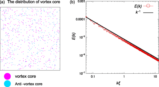
(a) Randomly distributed vortices (the uncorrelated turbulence). The total number of vortices is N v =686. (b) The energy spectrum E(k) with random vortices is obtained by making an ensemble average of 1000 times. Solid line shows k −1 (Color figure online)
-
2.
h +(l)≠h −(l) (The correlated turbulence)
In this case, Eq. (3) E(k) does not show E(k)∝k −1 in low wave number, because h +(l)≠h −(l) may lead to E int (k)≠0. We refer to this kind of turbulence to the correlated turbulence.

3 Two-Dimensional Quantum Turbulence of the Gross-Pitaevskii Equation
We show a simulation of the dimensionless GPE. As a method of making QT, this paper shows that 2D QT is created from many dark solitons through the dynamical instability [18, 19], which may occur in experiments when four BECs interfere.
We consider a dilute atomic BEC near zero temperature and atomic BECs are described by the condensate wave function \(\psi(\mathbf{r},\mathbf{t})=\sqrt{\mathbf{n}(\mathbf{r},\mathbf{t})}\exp(\mathbf{i}\theta( \mathbf{r},\mathbf{t}))\). The wave function ψ(r,t) obeys the dimensionless 2D GPE [17],
We numerically solve Eq. (8) in a uniform system by using the Crank-Nicholson method. n(r,t)=|ψ(r,t)|2 is the atomic number density of the condensate, m is a particle mass. The wave function, the coordinate and time are normalized by the bulk density n 0, the coherence length \(\xi = \hbar/\sqrt{2mn_{0}g_{2D}}\) and ħ/n 0 g 2D where g 2D is the strength of contact interaction of two particle in 2D systems. The system size is 256ξ×256ξ.
Figures 2(a), (b) and (c) show the time evolution of the condensate density n(r,t). We start the simulation with the initial stationary state obtained by the imaginary time step of the GPE in Fig. 2(a). The initial condition is that many dark solitons are arranged as a square grid of the interval 16ξ. We inject small random seeds for ψ(r) in order to trigger the instability of solitons. The unstable waves are excited along the solitons in Fig. 2(b). Then these solitons decay to a lot of vortices through the dynamical instability and lead to 2D QT with equal number of quantized vortices and anti-vortices which move around in the system in Fig. 2(c). Figure 2(d) shows the distribution of vortices at τ=112.5 where a time t is τ=t/(ħ/n 0 g 2D ).

(a–c) A time evolution of the condensate density |ψ(r,t)|2. Profile of the atomic number density at τ=0 (a). τ=56.25 (b), τ=112.5 (c), (d) the distribution of vorticity of the vortex and the anti-vortex τ=112.5 (Color figure online)
4 The Energy Spectrum of the Point Vortex Model and Correlation Functions
In order to determine whether 2D QT made by dark solitons is correlated or uncorrelated, we investigate the energy spectrum of the point vortex model and the correlation functions h ±(l).
The energy spectra of random vortices and 2D QT from dark solitons are shown in Fig. 3(a). Random distribution of vortices shows k −1 spectrum, while 2D QT such as made from decaying dark solitons can exhibit other spectral features and slopes in lower wave number than k l corresponding to the scale of the mean intervortex distance. These results denote that QT made from many dark solitons has the correlation of vortices, which is a type of different from the semi-classical turbulence because the spectrum of decaying dark solitons not agrees with the spectrum of semi-classical turbulence [20]. We show a time evolution of the energy spectra (Fig. 3(b)) and the correlation functions h ±(l) (Fig. 4). Figures 4(a) and (b) indicate that at τ=87.5 and τ=112.5 correlation of two vortices with like sign in l≤10 is weak due to h +(l) being smaller than h −(l). These results mean the binding of like sign vortices are less than that of opposite sign vortices. On the other hand, at τ=312.5, h +(l) approximately becomes h −(l), which is compared with maximum (Fig. 4(c)). This result means that the number of like sign pairs is comparable to that of the opposite sign pairs.

k l , k ξ and k soliton =2π/16ξ are the wave numbers corresponding to the mean intervortex distance \(l=\sqrt{N_{v}/S}\), the coherence length ξ and grid size 16ξ, respectively. (a) The energy spectrum of random vortices (Fig. 1(a)) and 2D QT (Fig. 2(d)) (N v =686). (b) Time evolution of the energy spectrum of 2D QT made from dark solitons at time τ=56.25, 87.5 and 312.5. The wave numbers corresponding to the mean intervortex distance are k l ξ≃0.92 (τ=56.25), 0.72 (τ=87.5) and 0.38 (τ=312.5). These energy spectra are obtained by the ensemble average of 10 times for discrimination of initial random seeds (Color figure online)

The correlation functions h ±(l) of the distance between two vortices with like sign and opposite sign. Here h ±(l) are normalized by unity. (a) τ=87.5 (N v =868), (b) τ=112.5 (N v =686) and (c) τ=312.5 (N v =238). Vertical dashed line shows 2ξ which means the minimum distance of two vortices (Color figure online)
One finds that a peak of the energy spectra (Fig. 3(b)) has shifted to the left as the vortices decay and the spectrum at τ=312.5 obeys E(k)∝k −1 in the lower wave number too, which means QT having a lot of opposite sign pairs gradually changes to the uncorrelated turbulence.
5 Summary
We discussed the configurations of vortices by calculating the energy spectra of superfluid velocity made by vortices and the correlation functions of the distance between two vortices. In this paper, it was found that 2D QT from dark solitons has a lot of opposite sign pairs which we call vortex pairs.
References
S.Z. Alamri et al., Phys. Rev. Lett. 101, 215302 (2008)
T.W. Neely et al., arXiv:1204.1102
B. Nowak et al., Phys. Rev. A 85, 043627 (2012)
N. Sasa et al., Phys. Rev. B 84, 054525 (2011)
P.M. Walmsley et al., Phys. Rev. Lett. 99, 265302 (2007)
W.F. Vinen, J. Low Temp. Phys. 161, 419 (2010)
D.I. Bradley et al., Phys. Rev. Lett. 96, 035301 (2006)
S. Fujiyama et al., Phys. Rev. B 81, 180512 (2010)
E. Kozik, B. Svistunov, Phys. Rev. B 77, 060502 (2008)
M. Kobayashi, M. Tsubota, J. Low. Temp. Phys. 145, 209–218 (2006)
R. Carretero-Gonzalez et al., Phys. Rev. A 77, 033625 (2008)
G. Ruben et al., Phys. Rev. A 78, 013631 (2008)
Y. Yatsuyanagi et al., Phys. Rev. Lett. 94, 054502 (2005)
Y. Yatsuyanagi, J. Plasma Fusion Res. Ser. 8, 931–935 (2009)
M.M. Sano et al., J. Phys. Soc. Jpn. 76, 064001 (2007)
A.S. Bradley, B.P. Anderson, arXiv:1204.1103
R. Numasato, M. Tsubota, Phys. Rev. A 81, 063630 (2010)
J. Brand, W.P. Reinhardt, Phys. Rev. A 65, 043612 (2005)
M. Ma et al., Phys. Rev. A 82, 023621 (2010)
A.W. Baggaley et al., Phys. Rev. B 85, 060501 (2012)
Author information
Authors and Affiliations
Corresponding author
Rights and permissions
Open Access This article is distributed under the terms of the Creative Commons Attribution License which permits any use, distribution, and reproduction in any medium, provided the original author(s) and the source are credited.
About this article
Cite this article
Kusumura, T., Takeuchi, H. & Tsubota, M. Energy Spectrum of the Superfluid Velocity Made by Quantized Vortices in Two-Dimensional Quantum Turbulence. J Low Temp Phys 171, 563–570 (2013). https://doi.org/10.1007/s10909-012-0827-9
Received:
Accepted:
Published:
Issue Date:
DOI: https://doi.org/10.1007/s10909-012-0827-9