Controlling Canard Cycles

Abstract

Canard cycles are periodic orbits that appear as special solutions of fast-slow systems (or singularly perturbed ordinary differential equations). It is well known that canard cycles are difficult to detect, hard to reproduce numerically, and that they are sensible to exponentially small changes in parameters. In this paper, we combine techniques from geometric singular perturbation theory, the blow-up method, and control theory, to design controllers that stabilize canard cycles of planar fast-slow systems with a folded critical manifold. As an application, we propose a controller that produces stable mixed-mode oscillations in the van der Pol oscillator.

1 Introduction

Fast-slow systems (also known as singularly perturbed ordinary differential equations, see more details in Section 2) are often used to model phenomena occurring in two or more time scales. Examples of these are vast and range from oscillatory patters in biochemistry and neuroscience [6, 18, 25, 26], all the way to stability analysis and control of power networks [10, 14], among many others [41, Chapter 20]. The overall idea behind the analysis of fast-slow systems is to separate the behavior that occurs at each time scale, understand such behavior, and then try to elucidate the corresponding dynamics of the full system. Many approaches have been developed, such as asymptotic methods [17, 34, 51, 52], numeric and computational tools [24, 32], and geometric techniques [20, 31, 33], see also [41, 46, 56]. In this article, we take a geometric approach.

Although the time scale separation approach has been very fruitful, there are some cases in which it does not suffice to completely describe the dynamics of a fast-slow system, see the details in Section 2. The reason is that, for some systems, the fast and the slow dynamics are interrelated in such a way that some complex behavior is only discovered when they are not fully separated. An example of the aforementioned situation are the so-called canards [7, 8, 15], see Section 2.1 for the appropriate definition. Canards are orbits that, counter-intuitively, stay close for a considerable amount of time to a repelling set of equilibrium points of the fast dynamics. Canards are extremely important not only in the theory of fast-slow systems, but also in applied sciences, and especially in neuroscience, as they have allowed, for example, the detailed description of the very fast onset of large amplitude oscillations due to small changes of a parameter in neuronal models [18, 26] and of other complex oscillatory patterns [9, 12, 47]. Due to their very nature, canard orbits are not robust, meaning that small perturbations may drastically change the shape of the orbit.

On the other hand, the application of singular perturbation techniques in control theory is far-reaching. Perhaps, as already introduced above, one of the biggest appeals of the theory of fast-slow systems is the time scale separation, which allows the reduction of large systems into lower dimensional ones for which the control design is simpler [29, 37, 38]. Applications range from the control of robots [28, 53, 54], all the way to industrial biochemical processes, and large power networks [13, 35, 36, 43, 49, 50]. However, as already mentioned, not all fast-slow systems can be analyzed by the convenient time scale separation strategy, and although some efforts from very diverse perspectives have been made [2,3,4,5, 22, 23, 29, 30], a general theory that includes not only the regulation problem but also the path following and trajectory planning problems is, to date, lacking.

The main goal of this article is to merge techniques of fast-slow dynamical systems with control theory methods to develop controllers that stabilize canard orbits. The idea of controlling canards has already been explored in [16], where an integral feedback controller is designed for the FitzHugh-Nagumo model to steer it towards the so-called canard regime. In contrast, here we take a more general and geometric approach by considering the folded canard normal form, see Section 2.1. Moreover, we integrate control techniques with Geometric Singular Perturbation Theory (GSPT) and propose a controller design methodology in the blow-up space. Later, we apply such geometric insight to the van der Pol oscillator where we provide a controller that produces any oscillatory pattern allowed by the geometric properties of the model, see Section 4.

The rest of this document is arranged as follows: in Section 2, we present definitions and preliminaries of the geometric theory of fast-slow systems and of folded canards, which are necessary for the main analysis. In Section 3, we develop a controller that stabilizes folded canard orbits, where the main strategy is to combine the blow-up method with state-feedback control techniques to achieve the goal. Afterwards in Section 4, as an extension to our previously developed controller, we develop a controller that stabilizes several canard cycles and is able to produce robust complex oscillatory patters in the van der Pol oscillator. We finish in Section 5 with some concluding remarks and an outlook.

2 Preliminaries

A fast-slow system is a singularly perturbed ordinary differential equation (ODE) of the form

$$ \begin{array}{ll} \varepsilon\dot x = f(x,y,\varepsilon,\lambda)\\ ~~\dot y = g(x,y,\varepsilon,\lambda), \end{array} $$

(1)

where $x\in \mathbb {R}^{m}$ is the fast variable, $y\in \mathbb {R}^{n}$ the slow variable, 0 < ε ≪ 1 is a small parameter accounting for the time scale separation between the aforementioned variables, $\lambda \in {\mathbb {R}}^{p}$ denotes other parameters, and f and g are assumed sufficiently smooth. In this document, the over-dot is used to denote the derivative with respect to the slow time τ. It is well-known that, for ε > 0, an equivalent way of writing Eq. 1 is

$$ \begin{array}{ll} x^{\prime} = f(x,y,\varepsilon,\lambda)\\ y^{\prime} = \varepsilon g(x,y,\varepsilon,\lambda), \end{array} $$

(2)

where now the prime denotes the derivative with respect to the fast time t := τ/ε.

One of the mathematical theories that is concerned with the analysis of Eqs. 1– 2 is Geometric Singular Perturbation Theory (GSPT) [41]. The overall idea of GSPT is to study the limit equations that result from setting ε = 0 in Eqs. 1– 2. Then, one looks for invariant objects that can be shown to persist up to small perturbations. Such invariant objects give a qualitative description of the behavior of Eqs. 1– 2. Accordingly, setting ε = 0 in Eqs. 1– 2 one gets

$$ \begin{array}{ll} 0 = f(x,y,0,\lambda)\qquad\qquad\qquad x^{\prime} = f(x,y,0,\lambda) \\ \dot y = g(x,y,0,\lambda) \qquad \qquad \qquad y^{\prime} = 0, \end{array} $$

(3)

known, respectively, as the reduced slow subsystem (which is a constrained differential equation [55] or a differential algebraic equation [42]) and the layer equation. The aforementioned limit systems are not equivalent any more, but they are related by the following important geometric object.

Definition 1 (The critical manifold)

The critical manifold is defined as

$$ \mathcal{C}_{0}=\left\{ (x,y)\in\mathbb{R}^{m}\times\mathbb{R}^{n} | f(x,y,0,\lambda)=0 \right\}. $$

(4)

We note that the critical manifold is the phase-space of the reduced slow subsystem and the set of equilibrium points of the layer equation. The properties of the critical manifold are essential to GSPT, in particular the following.

Definition 2 (Normal hyperbolicity)

Let $p\in \mathcal {C}_{0}$. We say that p is hyperbolic if the matrix $\text {D}_{x}f(p,0,\lambda )|_{\mathcal {C}_{0}}$ has all its eigenvalues away from the imaginary axis. If every point $p\in {\mathcal {C}}_{0}$ is hyperbolic, we say that ${\mathcal {C}}_{0}$ is normally hyperbolic. On the contrary, if for some $p\in {\mathcal {C}}_{0}$ the matrix ${\text {D}}_{x}f(p,0,\lambda )|_{{\mathcal {C}}_{0}}$ has at least one of its eigenvalues on the imaginary axis, then we say that p is a non-hyperbolic point.

It is known from Fenichel’s theory [19, 20] that a compact and normally hyperbolic critical manifold $\mathcal {S}_{0}\subseteq \mathcal {C}_{0}$ of Eq. 3 persists as a locally invariant slow manifold ${\mathcal {S}}_{{\varepsilon }}$ under sufficiently small perturbations. In other words, Fenichel’s theory guarantees that in a neighborhood of a normally hyperbolic critical manifold the dynamics of Eqs. 1–2 are well approximated by the limit systems Eq. 3.

Remark 1

Along this paper, we use the notation $\mathcal {S}_{0}^{\text {a}}$ and $\mathcal {S}_{0}^{\text {r}}$ to denote, depending on the eigenvalues of $\text {D}_{x}f(x,y,0,\lambda )|_{\mathcal {S}_{0}}$, the attracting an repelling parts of the (compact) critical manifold $\mathcal {S}_{0}$. Accordingly, the corresponding slow manifolds are denoted as $\mathcal {S}_{\varepsilon }^{\text {a}}$ and $\mathcal {S}_{\varepsilon }^{\text {r}}$.

On the other hand, critical manifolds may lose normal hyperbolicity, for example, due to singularities of the layer equation, see Fig. 1. It is in fact due to loss of normal hyperbolicity that, as in this paper, some interesting and complicated dynamics may arise in seemingly simple fast-slow systems. Fenichel’s theory, however, does not hold in the vicinity of non-hyperbolic points. In some cases, depending on the nature of the non-hyperbolicity, the blow-up method [27] is a suitable technique to analyze the complicated dynamics that arise. In the forthcoming section, we introduce the particular type of orbits that we are concerned with and that arise due to loss of normal-hyperbolicity of the critical manifold: the so-called canards.

Fig. 1

Singular flow of Eq. 7 near the origin. The gray parabola depicts the critical manifold $\mathcal {S}_{0}$ which is partitioned in its attracting $\mathcal {S}_{0}^{\text {a}}=\mathcal {S}_{0}|_{\left \{ x<0\right \}}$ and repelling $\mathcal {S}_{0}^{\text {r}}=\mathcal {S}_{0}|_{\left \{ x>0\right \}}$ parts, while the origin (the fold point) is non-hyperbolic. If α = 0, the origin is also called canard point. In this latter case, the orbit along the critical manifold is also known as singular maximal canard

2.1 Planar Folded Canards

In this section, we briefly describe folded canards and folded canard cycles in the plane. As we mention below, the adjective “folded” is due to a fold singularity. However, we remark that canards (and canard cycles) can be related to other types of singularities. The interested reader is refereed to, e.g. [15, 39, 57], references therein and, in particular, [41, Chapter 8] and [27, Section 3] for more detailed information.

Let us start by recalling that the canonical form of a canard point [39] is given by

$$ \begin{array}{ll} x^{\prime} = -y h_{1}(x,y,\varepsilon,\alpha) + x^{2}h_{2}(x,y,\varepsilon,\alpha) + \varepsilon h_{3}(x,y,\varepsilon,\alpha)\\ y^{\prime} = \varepsilon\left( xh_{4}(x,y,\varepsilon,\alpha)-\alpha h_{5}(x,y,\varepsilon,\alpha) +y h_{6}(x,y,\varepsilon,\alpha)\right), \end{array} $$

(5)

where $(x,y)\in \mathbb {R}^{2}$, 0 < ε ≪ 1, and α is a parameter. Furthermore,

$$ \begin{array}{ll} h_{3}(x,y,\varepsilon,\alpha) = \mathcal{O}(x,y,\varepsilon,\alpha)\\ h_{i}(x,y,\varepsilon,\alpha) = 1+\mathcal{O}(x,y,\varepsilon,\alpha),\qquad i=1,2,4,5, \end{array} $$

(6)

and h₆ is smooth. For simplicity of notation, we rewrite Eq. 5 together with Eq. 6 as

$$ \begin{array}{ll} x^{\prime} = -y+x^{2} + \widetilde f(x,y,\varepsilon,\alpha)\\ y^{\prime} = \varepsilon(x-\alpha + \widetilde g(x,y,\varepsilon,\alpha)), \end{array} $$

(7)

where $\widetilde f$ and $\widetilde g$ denote the corresponding higher order terms, that is:

$$ \begin{array}{ll} \widetilde f(x,y,\varepsilon,\alpha) := -y\mathcal{O}(x,y,\varepsilon,\alpha)+x^{2}\mathcal{O}(x,y,\varepsilon,\alpha)+\varepsilon\mathcal{O}(x,y,\varepsilon,\alpha),\\ \widetilde g(x,y,\varepsilon,\alpha) := x\mathcal{O}(x,y,\varepsilon,\alpha)-\alpha\mathcal{O}(x,y,\varepsilon,\alpha) +yh_{6}(x,y,\varepsilon,\alpha). \end{array} $$

(8)

The critical manifold is locally (near the origin) a perturbed parabola and is given by

$$ \mathcal{S}_{0} = \left\{ (x,y)\in\mathbb{R}^{2} | -y+x^{2}+ \widetilde f(x,y,0,\alpha)=0\right\}. $$

(9)

The (slow and fast) reduced flow corresponding to Eq. 7 is as shown in Fig. 1.

Remark 2

To fix ideas, consider for a moment Eq. 7 with zero higher order terms,¹ that is

$$ \begin{array}{ll} x^{\prime} = -y+x^{2}\\ y^{\prime} = \varepsilon(x-\alpha). \end{array} $$

(10)

Then, it is straightforward to check that, for ε > 0 and α = 0, the orbits of Eq. 10 are given by level sets of

$$ H(x,y,\varepsilon)=\frac{1}{2}\exp\left( -\frac{2y}{\varepsilon}\right)\left( \frac{y}{\varepsilon}-\frac{x^{2}}{\varepsilon}+\frac{1}{2} \right). $$

(11)

Some orbits of Eq. 10 are shown in Fig. 2, and in fact it is known [39] that canard cycles exist for $H\in (0,\frac {1}{4})$.

Fig. 2

Orbits of Eq. 10 obtained as level sets of Eq. 11. The dashed gray curve is the critical manifold. Compare with α = 0 in Fig. 1

What is remarkable is that there are orbits that closely follow the unstable branch of the critical manifold for slow time of order $\mathcal {O}(1)$. Such type of orbits are known as canards. There is a particular canard, which is called maximal canard and is given by $\left \{ H=0\right \}$ that connects the attracting slow manifold ${\mathcal {S}}_{{\varepsilon }}^{{\text {a}}}$ with the repelling one ${\mathcal {S}}_{{\varepsilon }}^{{\text {r}}}$. More relevant to this paper are periodic orbits with canard portions, which called canard cycles.

In the following section, we design feedback controllers for Eq. 5 that render a particular canard cycle asymptotically stable. In other words, we consider the path following control problem where a canard orbit is the reference.

3 Controlling Folded Canards

We propose to study two control problems, namely

$$ \begin{array}{ll} x^{\prime} = -y+x^{2}+ \widetilde f(x,y,\varepsilon,\alpha) +u(x,y,\varepsilon,\alpha)\\ y^{\prime} = \varepsilon(x-\alpha+\widetilde g(x,y,\varepsilon,\alpha)), \end{array} $$

(12)

which we call the fast control problem and

$$ \begin{array}{ll} x^{\prime} = -y+x^{2}+ \widetilde f(x,y,\varepsilon,\alpha) \\ y^{\prime} = \varepsilon(x-\alpha+\widetilde g(x,y,\varepsilon,\alpha)+u(x,y,\varepsilon,\alpha)), \end{array} $$

(13)

to be referred to as the slow control problem. Recall that $\widetilde f$ and $\widetilde g$ stand for the higher order terms as in Eq. 8. The objective is to stabilize a certain reference canard cycle to be denoted by γ_h.

Remark 3

• The choice of the above control problems is motivated by applications, especially in neuron models, see [16, 18, 26], where the input current appears in the fast (voltage) variable and regulates the distinct firing patterns. However, if one is interested in the fully actuated case, a combination of the techniques presented here shall also be useful.

• Throughout this document, we assume that one has full knowledge of the functions $\widetilde f$ and $\widetilde g$. This means that for the fast (resp. slow) control problem, we assume $\widetilde f=0$ (resp. $\widetilde g=0$). Otherwise, one considers a controller of the form $u=-\widetilde f+v$ (resp. $u=-\widetilde g+v$) where now v is to be designed.

Notice that in the case of the fast-control problem Eq. 12, the controller changes the fast dynamics. This means that the controller can change the type of singularities the critical manifold may present. To be more precise, consider for a moment Eq. 12 with u = −kx, k > 0, a simple proportional feedback controller. The closed-loop system then reads as

$$ \begin{array}{ll} x^{\prime} = -kx-y+x^{2}+ \widetilde f(x,y,\varepsilon,\alpha)\\ y^{\prime} = \varepsilon(x-\alpha+\widetilde g(x,y,\varepsilon,\alpha)), \end{array} $$

(14)

for which the origin is now normally hyperbolic. This means that the feedback controller has changed the type of singularity (at the origin) from a fold to a regular one. It is clear that these type of controllers are not compatible with our task. So, we shall design controllers that do not change the type of singularity of the open-loop system. To formalize what we mean by “not changing the type of singularity”, let us first recall the following definition:

Definition 3 (k-jet equivalence)

Let $F:\mathbb {R}^{n}\to \mathbb {R}^{n}$ and $G:\mathbb {R}^{n}\to \mathbb {R}^{n}$ be smooth maps. We say that F and G are (k-jet) equivalent at $p\in \mathbb {R}^{n}$ if F(p) = G(p) and $F(x)-G(x)=\mathcal {O}(||x-p||^{k+1})$ as x → p. An equivalence class defined by the previous notion of equivalence is called the k-jet of F at p, and shall be denoted by j^kF(p) [1].

Next, we have a formal definition of what we refer to as a compatible controller:

Definition 4 (Compatible controller)

Consider a control system

$$ \dot\zeta = f(\zeta,\lambda,u), $$

(15)

where $\zeta \in \mathbb {R}^{n}$ is the state variable, $\lambda \in \mathbb {R}^{p}$ denotes system parameters (possibly including 0 < ε ≪ 1), and $u\in \mathbb {R}^{m}$ stands for the controller. Suppose that for the open-loop system, that is when u = 0, the origin $\zeta =0\in \mathbb {R}^{n}$ is a nilpotent equilibrium point of $\dot \zeta = f(\zeta ,0,0)$ and that there is a $k\in \mathbb {N}$ such that k is the smallest number so that j^kf(0)≠ 0. Let u be a state-feedback controller, that is u = u(ζ,λ,ℓ), where $\ell \in \mathbb {R}^{m}$ stands for parameters of the controller such as controller gains, and denote by $\dot \zeta =F(\zeta ,\lambda ,\ell )$ the closed-loop system. We say that u is a compatible controller if the open-loop vector field f(ζ,λ,0) and the closed-loop vector field F(ζ,λ,ℓ) are k-jet equivalent at the origin for λ = 0.

We emphasize that once one fixes coordinates on $\mathbb {R}^{n}$, a k-jet equivalence between two maps means that such maps coincide on their partial derivatives up to order k. As an example of the above definition, recall that a planar fast-slow system with a generic fold at the origin is given by

$$ \begin{array}{ll} x^{\prime} = f(x,y,\varepsilon)\\ y^{\prime} = \varepsilon g(x,y,\varepsilon), \end{array} $$

(16)

with the defining conditions f(0,0,0) = 0, $\frac {\partial f}{\partial x}(0,0,0)=0$, $\frac {\partial ^{2} f}{\partial x^{2}}(0,0,0)\neq 0$, and the non-degeneracy condition $\frac {\partial f}{\partial y}(0,0,0)\neq 0$. Next, let u = u(x,y,ε) be a state-feedback controller and suppose one considers the fast-slow control system

$$ \begin{array}{ll} x^{\prime} = \underbrace{f(x,y,\varepsilon)+u(x,y,\varepsilon)}_{=:F(x,y,\varepsilon)}\\ y^{\prime} = \varepsilon g(x,y,\varepsilon). \end{array} $$

(17)

Then, u is a compatible controller if the closed-loop system verifies: F(0,0,0) = 0, $\frac {\partial F}{\partial x}(0,0,0)=0$, $\frac {\partial ^{2} F}{\partial x^{2}}(0,0,0)\neq 0$, and $\frac {\partial F}{\partial y}(0,0,0)\neq 0$, which implies that the controller does not change the class of the singularity, since the origin is still a fold point of the closed-loop system.

3.1 The Fast Control Problem

In this section, we study the control problem defined by

$$ \begin{array}{ll} x^{\prime} = -y + x^{2} + u(x,y,\varepsilon,\alpha)\\ y^{\prime} = \varepsilon(x-\alpha + \widetilde g(x,y,\varepsilon,\alpha)). \end{array} $$

(18)

Due to the fact that the slow dynamics are not actuated, we are going to stabilize canards centered at (x,y) = (α,0). Then, it is convenient to define ${\hat {x}}=x-\alpha$, which brings Eq. 18 into

$$ \begin{array}{ll} {\hat{x}}^{\prime} = -y+({\hat{x}}+\alpha)^{2}+{\hat{u}}({\hat{x}},y,\varepsilon,\alpha) \\ y^{\prime} = \varepsilon({\hat{x}}+{\hat{g}}({\hat{x}},y,\varepsilon,\alpha)), \end{array} $$

(19)

where ${\hat {u}}({\hat {x}},y,\varepsilon ,\alpha )=u({\hat {x}}+\alpha ,y,\varepsilon ,\alpha )$ and similarly for ${\hat {g}}$, we have ${\hat {g}}({\hat {x}},y,\varepsilon ,\alpha )=g({\hat {x}}+\alpha ,y,\varepsilon ,\alpha )$.

Theorem 1

Consider Eq. 19 and let $\hat H=H({\hat {x}},y,\varepsilon )$ be defined by Eq. 11. Then, the following hold:

• 1. The compatible controller

  $$ \hat u=-2\alpha{\hat{x}}-\alpha^{2}+c_{1}{\hat{x}}\varepsilon^{1/2}\exp(c_{2}y\varepsilon^{-1})(\hat H-h), $$

  (20)

  where c₁ > 0, $c_{2}\in \mathbb {R}$ and $h\leq \frac {1}{4}$, renders the canard orbit $\hat {\gamma }_{h}=\left \{ ({\hat {x}},y)\in \mathbb {R}^{2} | \hat H=h \right \}$ locally asymptotically stable for ε > 0 sufficiently small.

• 2. Let $\hat {{\varGamma }}\subset \mathbb {R}^{2}$ be a neigborhood of $\hat \gamma _{h}$ for $h\in (0,\frac {1}{4})$. Suppose that, additionally to Eq. 8, $\hat g$ is of the form $\hat g={\hat {x}}\hat \phi ({\hat {x}},y,{\varepsilon },\alpha )$ for some function $\hat \phi$, and that $\hat \phi \neq 1$ for all $(\hat x,y)\in \hat {{\varGamma }}$. Then, the compatible controller

  $$ \hat u=-2\alpha{\hat{x}}-\alpha^{2}+c_{1}{\hat{x}}\varepsilon^{1/2}(\hat H-h)\exp(c_{2}y\varepsilon^{-1})-(y-{\hat{x}}^{2})\hat\phi, $$

  (21)

  where c₁ > 0, $c_{2}\in \mathbb {R}$ renders the canard orbit $\hat {\gamma }_{h}=\left \{ ({\hat {x}},y)\in \mathbb {R}^{2} | \hat H=h \right \}$ locally (within $\hat {{\varGamma }}$) asymptotically stable.

Remark 4

• The choice of the controller gain c₂ in Theorem 1 has an important impact in numerical simulations due to the fact of it appearing as an argument of the exponential function. The choice c₂ = 2 yields the better numerical results when stabilizing canard cycles, that is for $h\in (0,\frac {1}{4})$. However, to stabilize the maximal canard (h = 0), it is necessary to choose c₂ < 2 to ensure that the controller remains bounded as $y\to \infty$. See more detail in Section 3.1.2.

• We recall that although from Theorem 1 one is able to stabilize any canard (because $h\leq \frac {1}{4}$), canard cycles exist only for $h\in (0,\frac {1}{4})$, see Fig. 2 and [39].

• The second item of Theorem 1 holds for any ε > 0.

The proof of Theorem 1 follows from the forthcoming analysis and is summarized in Section 3.1.3. We show in Fig. 3 a simulation of the results contained in Theorem 1.

Fig. 3

In all three columns we show, in the first row the $(\hat x,y)$ phase portrait of the closed-loop system Eq. 19 and in the second row the time-series of the corresponding controller. In all these simulations, ε = 0.01. (a) The case for which $\hat g=0$ and with parameters $(\alpha ,c_{1},c_{2},h)=(-0.1,1,2,\frac {1}{4}e^{-400})$. We remark here that in order for the constant $h=\frac {1}{4}e^{-400}$ to be numerically feasible, one has to input $h\exp (c_{2}y\varepsilon ^{-1})=\frac {1}{4}\exp (c_{2}y\varepsilon ^{-1}-400)$ into the numerical integration algorithm. The desired canard cycle to be followed is shown in dashed-gray. (b) The maximal canard case with $\hat g=0$ and with parameters (α,c₁,c₂,h) = (0,1,2 − e^− 15,0). Notice that, indeed, trajectories follow the unstable branch $\mathcal {S}_{\varepsilon }^{\text {r}}$ for a large “height” and that the corresponding controller remains bounded. (c) An example of the effect of the extra term in Eq. 21 where we show two trajectories with the same initial conditions. The unstable one is obtained with the controller Eq. 20 while the stable one with Eq. 21. The desired canard cycle to be followed is shown in dashed-gray. The large spike in the controller is observed every time the trajectory crosses the y-axis long a fast fiber. For such simulation, we have used $(\alpha ,c_{1},c_{2},h)=(0,5,2,\frac {1}{4}e^{-400})$ and g = 100x(y − x²). For more details, see Sections 3.1.1 and 3.1.2

As already anticipated, the idea is to design the controller ${\hat {u}}$ in the blow-up space. Therefore, let us consider a coordinate transformation defined by

$$ {\hat{x}}=\bar{r}\bar{x},\quad y=\bar{r}^{2}\bar{y}, \quad \varepsilon=\bar{r}^{2}\bar{{\varepsilon}}, \quad {\hat{u}}=\bar{r}^{2}\bar{\mu}, \quad \alpha=\bar{r}\bar{\alpha}, $$

(22)

where $(\bar {x},\bar {y},\bar {{\varepsilon }},\bar {\mu },\bar {\alpha })\in \mathbb {S}^{4}$, with $\mathbb {S}^{4}$ denoting the 4-sphere, that is $\{\bar {x}^{2}+\bar {y}^{2}+\bar {{\varepsilon }}^{2}+\bar {\mu }^{2}+\bar {\alpha }^{2}=1\}$, and $\bar {r}\in [0,\infty )$. As is usual with the blow-up method [27], instead of working in spherical coordinates, we consider local coordinates in local charts. In our particular context, these local charts parametrize different hemi-spheres of $\mathbb {S}^{4}$. Analogous to the analysis of the canard point in [39], we consider the charts $K_{1}=\left \{ \bar {y}=1 \right \}$ and $K_{2}=\left \{ \bar {{\varepsilon }}=1 \right \}$. To distinguish the local coordinates in these charts, we let (r₁,x₁,ε₁,μ₁,α₁) be local coordinates in K₁, and (r₂,x₂,y₂,μ₂,α₂) be local coordinates in K₂. In this way, these local coordinates are defined by:

$$ \begin{array}{ll} \!\!\!\!\!\!\!\!\!\!\!\!K_{1}\!:\! \quad {\hat{x}} = r_{1}x_{1}, \quad y = {r_{1}^{2}}, \quad\quad \varepsilon = {r_{1}^{2}}\varepsilon_{1}, \quad {\hat{u}} = {r_{1}^{2}}\mu_{1}, \quad \alpha = r_{1}\alpha_{1},\!\! \quad\qquad \text{{{for $y\!\geq\!0$}}}, \\ \!\!\!\!\!\!\!\!\!\!\!\!K_{2}\!:\! \quad {\hat{x}} = r_{2}x_{2}, \quad y = {r_{2}^{2}}y_{2}, \quad \varepsilon = {r_{2}^{2}}, \quad \quad {\hat{u}} = {r_{2}^{2}}\mu_{2}, \quad \alpha = r_{2}\alpha_{2},\!\! \quad\qquad \text{{{for $\varepsilon\!\geq\!0$}}}. \end{array} $$

(23)

In particular, it is worth noting that in chart K₁ the coordinate r₁ is a rescaling of the “original coordinate” y for y ≥ 0, while in chart K₂, the coordinate r₂ is a rescaling of ε ≥ 0. Furtheremore, in a qualitative sense, in chart K₁ one studies trajectories of Eq. 19 as they approach and leave a small neighborhood of the fold point in the positive y direction, while in chart K₂ one investigates the trajectories of Eq. 19 within a sufficiently small neighborhood of the fold point.

The coordinates in the above charts are related by the transition maps:

$$ \kappa_{12}:K_{1}\to K_{2}, \qquad r_{2} = r_{1}\varepsilon_{1}^{1/2}, x_{2} = x_{1}\varepsilon_{1}^{-1/2}, y_{2}=\varepsilon_{1}^{-1}, \mu_{2} = \mu_{1}\varepsilon_{1}^{-1}, \alpha_{2}=\alpha_{1}\varepsilon_{1}^{-1/2}, $$

(24)

for ε₁ > 0 and

$$ \kappa_{21}:K_{2}\to K_{1},\qquad r_{1} = r_{2}y_{2}^{1/2}, x_{1} = x_{2}y_{2}^{-1/2}, \mu_{1}=\mu_{2}y_{2}^{-1}, \varepsilon_{1}=y_{2}^{-1}, \alpha_{1} = \alpha_{2}y_{2}^{-1/2}, $$

(25)

for y₂ > 0.

3.1.1 Analysis in the Rescaling Chart K ₂

The blown-up (and desingularized) local vector field in this chart reads as

$$ \begin{array}{ll} x^{\prime}_{2} = -{y}_{2} + ({x}_{2}+{\alpha}_{2})^{2} + {\mu}_{2} \\ y^{\prime}_{2} = {x}_{2} + {g_{2}}, \end{array} $$

(26)

where g₂ = g₂(r₂,x₂,y₂,α₂) is smooth and defined by the blow-up of $\hat g$. More precisely, from Eq. 8 and keeping in mind the usual desingularization step, one has that

$$ {g_2}={x}_{2}\mathcal{O}({r}_{2}{x}_{2},{r}_{2}^{2}{y}_{2},{r}_{2}^{2},{r}_{2}{\alpha}_{2})+{\alpha}_{2}\mathcal{O}({r}_{2}{x}_{2},{r}_{2}^{2}{y}_{2},{r}_{2}^{2},{r}_{2}{\alpha}_{2})+{r}_{2}{y}\bar h_{6}({x}_{2},{y}_{2},{r}_{2},{\alpha}_{2}), $$

(27)

where $\bar h_{6}$ is smooth. Then, it is clear that $g_{2}\in \mathcal {O}({r}_{2})$. Similarly, μ₂ = μ₂(x₂,y₂,r₂,α₂) is the blown-up state-feedback controller to be designed. Observe that, analogously to what is described in Remark 2, we have that for ${\bar {r}}={\bar {\alpha }}={\bar {\mu }}=0$ the orbits of Eq. 26 are given as level sets of the function

$$ H_{2}({x}_{2},{y}_{2}) = \frac{1}{2}\exp(-2{y}_{2})\left( {y}_{2}-{x}_{2}^{2}+\frac{1}{2}\right). $$

(28)

Having this in mind, we are going to design μ₂ in such a way that for a trajectory (x₂(t₂),y₂(t₂)) of Eq. 26 one has $\lim _{t_{2}\to \infty } H_{2}({{x}_{2}}(t_{2}),{{y}_{2}}(t_{2}))= h$, where h defines the desired canard cycle and t₂ denotes the time-parameter of Eq. 26.

We approach the design of μ₂ as follows: we start by restricting to $\left \{ \bar {r}=0 \right \}$ and define $\widetilde {H}_{2}=H_{2}-h$, where $h\in (0,\frac {1}{4})$.² Next, we define a candidate Lyapunov function given by

$$ L_{2}({x}_{2},{y}_{2})=\frac{1}{2}\widetilde{H}_{2}^{2}, $$

(29)

and note that L₂ > 0 for all $\widetilde {H}_{2}\neq 0$ and that L₂ = 0 if and only if $\widetilde {H}_{2}=0$, if and only if (x₂,y₂) ∈ γ_h, where by γ_h we denote the reference canard cycle, that is

$$ \gamma_{h}=\left\{ ({x}_{2},{y}_{2})\in\mathbb{R}^{2} | \widetilde{H}_{2}=0 \right\}. $$

(30)

It follows that

$$ L_{2}^{\prime}=-{x}_{2}\exp(-2{y}_{2})\widetilde{H}_{2}\left( 2\bar{\alpha}{x}_{2} + \bar{\alpha}^{2} + {\mu}_{2}^{0} \right), $$

(31)

where ${\mu }_{2}^{0}={\mu }_{2}(0,{x}_{2},{y}_{2},\bar {\alpha })$. Naturally, we want to design ${\mu }_{2}^{0}$ such that $L_{2}^{\prime }<0$, or at least $L_{2}^{\prime }\leq 0$. We now see that a convenient choice of ${\mu }_{2}^{0}$ is

$$ {\mu}_{2}^{0} = -2\bar{\alpha}{x}_{2} - \bar{\alpha}^{2} + c_{1}{x}_{2}\exp(c_{2}{y}_{2})\widetilde{H}_{2}, $$

(32)

where c₁ > 0 and $c_{2}\in \mathbb {R}$ are the controller gains. Using Eq. 32 we have

$$ L_{2}^{\prime} = -c_{1}{x}_{2}^{2}\exp((c_{2}-2){y}_{2})\widetilde{H}_{2}^{2}\leq0. $$

(33)

Note that, because the exponential function is positive, the previous inequality holds for every value of $c_{2}\in \mathbb {R}$; however, a particular choice of c₂ may drastically change the performance of the controller, hence its inclusion in Eq. 32. This can be readily seen if we substitute $\widetilde {H}_{2}$ in Eq. 32:

$$ {\mu}_{2}^{0} = -2\bar{\alpha}{x}_{2} - {\alpha}^{2}_{2} + \frac{1}{2}c_{1}{x}_{2}\exp((c_{2}-2){y}_{2})\left( {y}_{2}-{x}_{2}^{2}+\frac{1}{2}\right)-c_{1}{x}_{2}\exp(c_{2}{y}_{2})h. $$

(34)

Let $D\subset \mathbb {R}^{3}$ be a bounded domain. We see that ${\mu _{2}^{0}}$ is bounded for all $(\bar {\alpha },{x}_{2},{y}_{2})\in D$. However, since c₂ appears inside the exponential, the upper bound of $|{\mu _{2}^{0}}|$ can vary widely depending on the choice of c₂. The relevance of c₂ shall be detailed in Section 3.1.2.

By Lasalle’s invariance principle [44] we have that, under the controller Eq. 32 and r₂ = 0, the trajectories of Eq. 26 eventually reach the largest invariant set contained in

$$ \mathcal{I}=\left\{ ({x}_{2},{y}_{2})\in\mathbb{R}^{2} | L_{2}^{\prime}=0\right\}=\left\{ {x}_{2}=0 \right\}\cup\left\{ \widetilde{H}_{2}=0 \right\} $$

(35)

Note, however, that $\left \{ {x}_{2}=0 \right \}$ is generically not invariant for the closed-loop dynamics Eq. 26. Indeed, the closed-loop system Eq. 26 (restricted to r₂ = 0) reads as

$$ \begin{array}{@{}rcl@{}} {x}_{2}^{\prime} &=& -{y}_{2} + {x}_{2}^{2} + c_{1}{x}_{2}\exp(c_{2}{y}_{2})\widetilde{H}_{2} \\ {y}_{2}^{\prime} &=& {x}_{2}, \end{array} $$

(36)

where setting x₂ = 0 leads to $({x}_{2}^{\prime },{y}_{2}^{\prime })=(-{y}_{2},0)$. Therefore, we now have that all trajectories of Eq. 26 eventually reach $\mathcal {I}_{2}=\left \{ ({x}_{2},{y}_{2})=(0,0) \right \}\cup \left \{ \widetilde {H}_{2}=0 \right \}$. Since the origin is an equilibrium point of Eq. 36,³ we have that every trajectory with initial conditions $({x}_{2}(0),{y}_{2}(0))\in \mathbb {R}^{2}\backslash \left \{ (0,0) \right \}$ eventually reaches the set $\left \{\widetilde {H}_{2}=0\right \}$ as $t_{2}\to \infty$. With the previous analysis we have shown the following:

Proposition 1

Consider Eq. 26. Then, for r₂ ≥ 0 sufficiently small a controller of the form

$$ {\mu}_{2} = -2{\alpha}_{2}{x}_{2}-{\alpha}^{2}_{2} + c_{1}{x}_{2}\exp(c_{2}{y}_{2})\left( H_{2}-h \right) +\mathcal{O}({r}_{2}), $$

(37)

where c₁ > 0 and $c_{2}\in \mathbb {R}$ and with H₂ is as in Eq. 28, renders the orbit γ_h locally asymptotically stable.

Proof

As described above, the stability of γ_h for Eq. 37 is equivalent to the stability of the zero solution of

$$ \tilde H_{2}^{\prime}=-{x}_{2}\exp(-2{y}_{2})(2{\alpha}_{2}{x}_{2}+{\alpha}^{2}_{2}+{\mu_{2}^{0}})+\mathcal{O}({r}_{2}). $$

(38)

Substituting Eqs. 32 in 38 we get

$$ \tilde H_{2}^{\prime}= -c_{1}{x}_{2}^{2}\exp((c_{2}-{y}_{2}))\tilde H_{2}+\mathcal{O}({r}_{2}). $$

(39)

We have shown that for r₂ = 0, the origin is locally asymptotically stable for Eq. 39. An apparent issue in Eq. 39 is the term ${x_{2}^{2}}$. However, we have also shown that $\left \{ {x}_{2}=0 \right \}$ is not invariant. Therefore, Eq. 39 is a particular case of the non-autonomous scalar equation

$$ \tilde H_{2}^{\prime}=-a(t_{2})\tilde H_{2}+\mathcal{O}({r}_{2}), $$

(40)

where a(t₂) ≥ 0 for all t₂ anda(t₂) > 0 for almost all t₂ (here t₂ is the time parameter in the chart K₂). The solution of the unperturbed Eq. 40 is $H_{2}(t_{2})=k \exp \left (-{\int \limits }_{t_{0}}^{t_{2}}a(s_{2})\text {d}s_{2} \right )$, for some $k\in \mathbb {R}$. So, due to the properties of a(t₂), the trivial solution of Eq. 40, with r₂ = 0, is asymptotically stable, which is preserved under sufficiently small perturbations $\mathcal {O}({r}_{2})$ [11]. □

We show in Fig. 4 a simulation of the result postulated in Proposition 1.

Fig. 4

Simulation of Eq. 26 with the controller Eq. 32. The parameters for the simulation are (r₂,α₂,c₁, c₂,h) = (0,1,1,2,1 × 10^− 16). The desired periodic orbit is depicted as the dashed curve

Let us emphasize at this point that designing the controller in the rescaling chart justifies using H₂ to define a convenient Lyapunov function, even if there are higher order terms in the original vector field Eq. 19. We also point out that the maximal canard becomes unbounded in this chart. Such a case shall be studied in chart K₁ (see Section 3.1.2 below). Next we digress on how to deal with a certain class of higher order terms even if r₂ (equivalently ε) is not small.

Lemma 1

Consider Eq. 26 with r₂ > 0 fixed and let ${{\varGamma }}_{2}\subset \mathbb {R}^{2}$ be a neighbourhood of γ_h. Assume that the function g₂ satisfies

• 1. g₂ = x₂ϕ₂(r₂,x₂,y₂,α₂), where ϕ₂ is smooth and vanishes at the origin.

• 2. The function ϕ₂ satisfies 1 + ϕ₂(r₂,0,y₂,α₂)≠ 0 for all (0,y₂) ∈Γ₂.

• 3. The function ϕ₂ satisfies 1 + ϕ₂(r₂,x₂,y₂,α₂)≠ 0 for all (x₂,y₂) ∈ γ_h.

Then, a controller of the form

$$ {\mu}_{2} = -2{\alpha}_{2}{x}_{2}-{\alpha}^{2}_{2} + c_{1}{x}_{2}\exp(c_{2}{y}_{2})\left( H_{2}-h \right) - ({y}_{2}-{x}_{2}^{2}){\phi_{2}}, $$

(41)

where c₁ > 0 and $c_{2}\in \mathbb {R}$, renders γ_h locally asymptotically stable in Γ₂.

Proof

First, we recall that $g_{2}\in \mathcal {O}({r}_{2})$, see Eq. 27. Therefore, under the assumptions of the Lemma we can write g₂ = x₂ϕ₂ = r₂x₂ψ₂ for some function ψ₂. Next, and similar to the analysis performed above, we consider Eq. 26 but now with an extra $\mathcal {O}({r}_{2})$-term in the controller, namely

$$ \begin{array}{ll} {x}_{2}^{\prime} = -{y}_{2} + ({x}_{2}+{\alpha}_{2})^{2} + {\mu}_{2}^{0} + {r}_{2}{v}_{2} \\ {y}_{2}^{\prime} = {x}_{2} + {g_2}, \end{array} $$

(42)

where ${\mu }_{2}^{0}$ is as in Eq. 32 and now v₂ = v₂(r₂,x₂,y₂,α₂) is to be designed. Consider, as before, the candidate Lyapunov function Eq. 29. After substituting ${\mu }_{2}^{0}$ and g₂ = r₂x₂ψ₂, we get

$$ L_{2}^{\prime}= -c_{1}{x}_{2}^{2}\widetilde{H}_{2}^{2}\exp((c_{2}-2){y}_{2}) - {r}_{2}{x}_{2}\widetilde{H}_{2}\exp(-2{y}_{2})({v}_{2}+({y}_{2}-{x}_{2}^{2}){{{\psi_{2}}}}). $$

(43)

The above expression suggests to set ${v}_{2}=-(y-{x}_{2}^{2}){{{\psi _{2}}}}$. By doing so one gets Eq. 31 again and therefore, invoking again Lasalle’s invariance principle, we now take a look at the set ${\mathcal {I}}=\left \{ {{x}_{2}}=0 \right \}\cup \left \{ \widetilde {H}_{2}=0 \right \}$ related to the closed-loop system. To be more precise we now focus on

$$ \begin{array}{ll} {x}_{2}^{\prime} = -{y}_{2} + {x}_{2}^{2} + c_{1}{x}_{2}\exp(c_{2}{y}_{2})\widetilde{H}_{2} - ({y}_{2}-{x}_{2}^{2}){\phi_{2}}\\ {y}_{2}^{\prime} = {x}_{2} + {x}_{2}{\phi_{2}}, \end{array} $$

(44)

where we have used r₂ψ₂ = ϕ₂, and consider its dynamics restricted to $\mathcal {I}$. On $\left \{ {x}_{2}=0 \right \}$ one has $({x}_{2}^{\prime },{y}_{2}^{\prime })=\left (-{y}_{2}\left (1+{\phi _{2}}|_{\left \{ {x}_{2}=0 \right \}}\right ),0\right )$. Therefore, to avoid $\left \{ {x}_{2}=0 \right \}$ being invariant we impose the condition 1 + ϕ₂(r₂,0,y₂,α₂)≠ 0. Note that the aforementioned condition would already suffice to show that trajectories converge towards $\left \{ \widetilde {H}_{2}=0 \right \}$; however, there may still be a stable equilibrium point contained in $\left \{ \widetilde {H}_{2}=0 \right \}$. The restriction of Eq. 44 to $\left \{ \widetilde {H}_{2}=0 \right \}$ reads as

$$ \begin{array}{ll} {x}_{2}^{\prime} = (-{y}_{2} + {x}_{2}^{2})(1+ {\phi_{2}}) \\ {y}_{2}^{\prime} = {x}_{2}(1 + {\phi_{2}}), \qquad\qquad ({x}_{2},{y}_{2})\in\gamma_{h}. \end{array} $$

(45)

Now it suffices to give conditions on ${\phi _{2}}|_{\left \{({x}_{2},{y}_{2})\in \gamma _{h}\right \}}$ such that Eq. 45 does not have equilibrium points (keep in mind that (0,0)∉γ_h for h ∈ (0,1/4)). Such a condition is simply 1 + ϕ₂(r₂,x₂,y₂,α₂)≠ 0 for all (x₂,y₂) ∈ γ_h, completing the proof. □

Remark 5

• If the third assumption of Lemma 1 does not hold, then trajectories converge to an equilibrium point contained in the set $\left \{\widetilde {H}_{2}=0\right \}$.

• A simpler to check and sufficient condition on ϕ₂ satisfying the hypothesis of Lemma 1 is ϕ₂(r₂,x₂,y₂,α₂)≠ 1 for all (x₂,y₂) ∈Γ₂. Also, if g = xϕ(x,y,ε,α) and g₂ = x₂ϕ₂ is its blown-up version, then ${\phi _{2}}({{r}_{2}},{{x}_{2}},{{y}_{2}},{{\alpha }_{2}})=\phi ({{r}_{2}}{{x}_{2}},{{r}_{2}}^{2}{{y}_{2}},{{r}_{2}}^{2},{{r}_{2}}{{\alpha }_{2}})=\phi (x,y,{\varepsilon },\alpha )$. Therefore, ϕ₂≠ 1 implies ϕ≠ 1. These two arguments are the ones we use for Theorem 1.

We show in Fig. 5 a simulation regarding Lemma 1.

Fig. 5

An example of a phase portrait corresponding to Eq. 26 with the particular choice: r₂ = 1, α₂ = 1, ${\phi _{2}}={y}_{2}-{x}_{2}^{2}$ and (c₁,c₂) = (10,2). Due to the way the local coordinates in this chart are defined, choosing r₂ = 1, essentially amounts to considering ε = 1 in Eq. 19. On the left, we show the orbits corresponding to v₂ = 0, and on the right, those for v₂ given as in Lemma 1. Observe on the left that trajectories do not follow the desired canard while on the right they do. This means that the extra term v₂ is suitable to render the canard asymptotically stable when the perturbations of order $\mathcal {O}({r}_{2})$ in Eq. 26 are not small

3.1.2 Analysis in the Directional Chart K1

We are now going to look at the controlled dynamics in the chart K₁. This serves two purposes: the first is of giving a more precise meaning to the constant c₂ in the controller Eq. 37; the second is to corroborate that the controller designed previously is indeed able to also stabilize the (unbounded) maximal canard. Using the definition on K₁ as in Eq. 23, we have that the dynamics in this chart read as

$$ \begin{array}{llll} {r}_{1}^{\prime} = \frac{1}{2}{r}_{1}{{\varepsilon}}_{1}{x}_{1}+\mathcal{O}({r}_{1}{{\varepsilon}}_{1})\\ {x}_{1}^{\prime} = -1+({x}_{1}+{\alpha}_{1})^{2}-\frac{1}{2}{{\varepsilon}}_{1}{x}_{1}^{2}+{\mu}_{1}+\mathcal{O}({r}_{1}{{\varepsilon}}_{1})\\ {{\varepsilon}}_{1}^{\prime} =-{{\varepsilon}}_{1}^{2}{x}_{1}+\mathcal{O}({r}_{1}{{\varepsilon}}_{1})\\ {\alpha}_{1}^{\prime} =-\frac{1}{2}{{\varepsilon}}_{1}{x}_{1}+\mathcal{O}({r}_{1}{{\varepsilon}}_{1}), \end{array} $$

(46)

where, in particular, μ₁ denotes the controller written in the local coordinates of this chart. Since we have already designed a controller in the chart K₂, see Eq. 37, we can use the transformation Eq. 25 to express μ₁ as

$$ {\mu}_{1} =\kappa_{21}(\mu_{2})=-2{\alpha}_{1}{x}_{1}-{\alpha}^{2}_{1}+c_{1}{{\varepsilon}}_{1}^{1/2}{x}_{1}\exp(c_{2}{{\varepsilon}}_{1}^{-1})\widetilde{H}_{1}+\mathcal{O}({r}_{1}{{\varepsilon}}_{1}^{3/2}), $$

(47)

where, analogous to what we have done in chart K₂, we define $\widetilde {H}_{1}=H_{1}-h$ with

$$ H_{1} = \kappa_{21}(H_{2}) = \frac{1}{2}\exp\left( -2{{\varepsilon}}_{1}^{-1}\right)\left( {{\varepsilon}}_{1}^{-1}-{{\varepsilon}}_{1}^{-1}{x}_{1}^{2}+\frac{1}{2}\right). $$

(48)

Remark 6

• μ₁ is bounded along any reference canard $\gamma _{h}=\left \{ \widetilde {H}_{1}=0\right \}$ with $h\in (0,\frac {1}{4})$.

• If h≠ 0, then μ₁ becomes unbounded as ε₁ → 0 unless $\widetilde {H}_{1}=0$ (previous observation). This is to be expected as, in the limit ε₁ → 0 the only canard orbit to stabilize is the maximal canard since $\lim _{{{{\varepsilon }}_{1}}\to 0}H_{1}=0$. Therefore, we are going to study the closed-loop dynamics Eq. 46 for the particular choice of h = 0 and for the limit ε₁ → 0. Our goal is to refine the constant c₂ so that μ₁ remains bounded whenever h = 0 and ε₁ → 0. Moreover, recalling that for this chart we have ${{{\varepsilon }}_{1}}=\frac {y}{{\varepsilon }}$, the limit ε₁ → 0 corresponds to the limit $y\to \infty$ for fixed ε > 0.

So from now on, we let h = 0, that is $\widetilde {H}_{1}=H_{1}=\frac {1}{2}\exp \left (-2{{\varepsilon }}_{1}^{-1}\right )\left ({{\varepsilon }}_{1}^{-1}-{{\varepsilon }}_{1}^{-1}{x}_{1}^{2}+\frac {1}{2}\right )$. We also restrict to $\left \{{r}_{1}=0 \right \}$. In such a case we have

$$ {\mu}_{1}=-2{\alpha}_{1}{x}_{1}-{\alpha}^{2}_{1}+\frac{1}{2}c_{1}{{\varepsilon}}_{1}^{1/2}{x}_{1}\exp\left( (c_{2}-2){{\varepsilon}}_{1}^{-1}\right)\left( {{\varepsilon}}_{1}^{-1}-{{\varepsilon}}_{1}^{-1}{x}_{1}^{2}+\frac{1}{2}\right), $$

(49)

and the closed loop system reads as

$$ \begin{array}{lll} {x}_{1}^{\prime} = -1+{x}_{1}^{2}-\frac{1}{2}{{\varepsilon}}_{1}{x}_{1}^{2}+\frac{1}{2}c_{1}{{\varepsilon}}_{1}^{1/2}{x}_{1}\exp(c_{2}{{\varepsilon}}_{1}^{-1})H_{1}\\ {{\varepsilon}}_{1}^{\prime} = -{{\varepsilon}}_{1}^{2}{x}_{1}\\ {\alpha}_{1}^{\prime} = -\frac{1}{2}{{\varepsilon}}_{1}{x}_{1}. \end{array} $$

(50)

It shall also be relevant to consider $H_{1}^{\prime }$, namely

$$ \begin{array}{ll} H_{1}^{array} = -\frac{1}{2}c_{1}{{\varepsilon}}_{1}^{-1/2}{x}_{1}^{2}\exp\left( (c_{2}-2){{\varepsilon}}_{1}^{-1}\right)H_{1}\\ ~~~~~~~~~~~~=-\frac{1}{2}c_{1}{{\varepsilon}}_{1}^{-1/2}{x}_{1}^{2}\exp\left( (c_{2}-4){{\varepsilon}}_{1}^{-1}\right)\left( {{\varepsilon}}_{1}^{-1}-{{\varepsilon}}_{1}^{-1}{x}_{1}^{2}+\frac{1}{2}\right). \end{array} $$

(51)

First of all, we note that $\lim _{{{\varepsilon }}_{1}\to 0} H_{1}=0$, and $\lim _{{{\varepsilon }}_{1}\to 0} H_{1}^{\prime }=0$ for c₂ < 4. Next, we focus on Eq. 49 where we observe that in order for the controller to be bounded as ε₁ → 0the constant c₂ should be less than 2. To be more precise:

Lemma 2

Let (α₁,x₁) be bounded and c₁ > 0. Then, $\lim _{{{\varepsilon }}_{1}\to 0}|{\mu }_{1}|<\infty$ if and only if c₂ < 2.

Proof

Straightforward computations. □

From Lemma 2 we have that, to follow the maximal canard (h = 0) one must choose c₂ < 2 to ensure that the controller is bounded. Although analytically any choice of c₂ < 2 suffices, a particular choice may influence drastically numerical simulations since c₂ appears in the exponential. For instance, we see from the first line of Eq. 51 that c₂ < 2 but arbitrarily close to 2 reduces the contribution of the exponential term, which may induce issues in numerical simulations. For all other canards, $c_{2}\in \mathbb {R}$ is sufficient. However, again from the computational perspective, c₂ = 2 is the appropriate choice as it eliminates the exponential term in Eq. 49 and in Eq. 51, which is rather convenient for simulations. We remark that a completely analogous analysis, which we omit for brevity, follows for the chart $K_{3}=\left \{ \bar x=1 \right \}$ where canards corresponding to h < 0 can be considered. The arguments and the conclusion are the same, namely, for h < 0 one should set c₂ < 2 so that the controller remains bounded along the unbounded canards.

3.1.3 Proof of Theorem 1

To prove Theorem 1, we first blow-down the controller μ₁. To keep it simple, we shall blow-down Eq. 37, but of course the same holds for Eq. 41. So, recall from Eq. 37 that the blown-up controller is

$$ {\mu}_{2}=-2{\alpha}_{2}{x}_{2}-{\alpha}^{2}_{2} + c_{1}{x}_{2}\exp(c_{2}{y}_{2})\left( H_{2}-h \right). $$

(52)

Next, from Eq. 23, we have

$$ \hat u=\varepsilon {\mu}_{2} = -2\alpha{\hat x} - \alpha^{2} + c_{1}{\hat x}\varepsilon^{1/2}\exp\left( c_{2}y\varepsilon^{-1}\right)(\hat H-h), $$

(53)

where $\hat H=\hat H({\hat x},y,\varepsilon )=\frac {1}{2}\exp \left (-\frac {2y}{\varepsilon }\right )\left (\frac {y}{\varepsilon }-\frac {{\hat x}^{2}}{\varepsilon }+\frac {1}{2} \right )$ as stated in the first item of Theorem 1. Under Eq. 53, the closed-loop system corresponding to Eq. 19 reads as

$$ \begin{array}{ll} {\hat x}^{\prime} = -y+{\hat x}^{2} + c_{1}{\hat x}\varepsilon^{1/2}\exp\left( c_{2}y\varepsilon^{-1}\right)(\hat H-h)\\ y^{\prime} = \varepsilon({\hat x}+\widetilde g). \end{array} $$

(54)

Next, it is important to observe that $\lim _{\varepsilon \to 0}\hat H=0$. This means that for ε = 0 the only reference canard that is reachable is the maximal canard.⁴ The maximal canard corresponds to h = 0. So, setting h = 0, and since one chooses c₂ < 2 (recall Section 3.1.2), it follows that $\lim _{{\varepsilon }\to 0}c_{1}{\hat x}{\varepsilon }^{1/2}\exp \left (c_{2}y{\varepsilon }^{-1}\right )\hat H=0$, meaning that the layer equation for Eq. 54 is

$$ \begin{array}{ll} {\hat x}^{\prime} = -y+{\hat x}^{2} \\ y^{\prime} = 0, \end{array} $$

(55)

which indeed has the same type of singularity at the origin as the open-loop system, a fold. This shows that Eq. 53 is a compatible controller in the sense of Definition 4.

3.2 The Slow Control Problem

In this section, we consider the slow-control problem

$$ \begin{array}{ll} x^{\prime} = -y+x^{2}+ f(x,y,\varepsilon,\alpha) \\ y^{\prime} = \varepsilon(x-\alpha+u(x,y,\varepsilon,\alpha)), \end{array} $$

(56)

where the objective is, as in Section 3.1, to stabilize a prescribed canard γ_h. Due to space constraints, and because the analysis is similar to the one performed in Section 3.1, we only state the relevant result.

Theorem 2

Consider Eq. 56 and let $\hat H=H(x,y,\varepsilon )$ be defined by Eq. 11. Then, the compatible controller

$$ u=\alpha+c_{1}(y-x^{2})\varepsilon^{-1/2}\exp(c_{2}y\varepsilon^{-1})(H-h), $$

(57)

where c₁ > 0, $c_{2}\in \mathbb {R}$ and $h\leq \frac {1}{4}$ renders the canard orbit $\gamma _{h}=\left \{ (x,y)\in \mathbb {R}^{2} | H=h \right \}$ locally asymptotically stable for ε > 0 sufficiently small. A convenient choice of controller gain c₂ for the maximal canard is c₂ < 2. By convenient we mean that such a choice ensures that the controller remains bounded as $y\to \infty$.

In Fig. 6, we illustrate the statement of Theorem 2.

Fig. 6

The first column corresponds to the control of a bounded canard cycle (shown in dashed-gray), while the second column to the control of the maximal canard. The first row shows the phase-portrait in (x,y)-coordinates. The second row shows the time series of the corresponding controller. We show on the lower-right diagram a detail of the controller’s signal for time close to 0

4 Controlling Canard Cycles for the Van Der Pol Oscillator

In this section, we are going to extend the ideas developed previously to control canard cycles in the van der Pol oscillator. The main idea is to adapt and extend the controller proposed in Theorem 1, and to use it to control canard cycles of the van der Pol oscillator. In this context, we distinguish two types of canard cycles: (a) canards with head and (b) canards without head. Canards with head refer to canard cycles with two fast segments, while canards without head have only one fast segment, see Fig. 8. Furthermore, due to its relationship with some neuron models, like the Fitzhugh-Nagumo model [21, 48], we shall consider that the controller acts on the fast variable only. The idea is that the controller represents input current. Thus, let us study

$$ \begin{array}{ll} x^{\prime} = -y+x^{2}-\frac{1}{3}x^{3}+u \\ y^{\prime} = \varepsilon x. \end{array} $$

(58)

Remark 7

For simplicity, we have chosen to present the case α = 0. However, the case α≠ 0 follows straightforwardly from considering the arguments at the beginning of Section 3.1.

The corresponding critical manifold reads as,

$$ \mathcal{S}_{0} = \left\{ (x,y)\in\mathbb{R}^{2} : y=x^{2}-\frac{1}{3}x^{3}\right\}. $$

(59)

The repelling and attracting parts of $\mathcal {S}_{0}$ are denoted respectively by $\mathcal {S}_{0}^{\text {r}}$ and $\mathcal {S}_{0}^{\text {a}}$, and are given by

$$ \begin{array}{ll} \mathcal{S}_{0}^{\text{r}} = \left\{ (x,y)\in\mathcal{S}_{0} : 0<x<2\right\}\\ \mathcal{S}_{0}^{\text{a}} = \left\{ (x,y)\in\mathcal{S}_{0} : x<0\right\}\cup\left\{ (x,y)\in\mathcal{S}_{0} : x>2\right\}. \end{array} $$

(60)

Furthermore, system Eq. 58 has two fold points, one at the origin and one at $(x,y)=(2,\frac {4}{3})$. In fact, the origin is a canard point and the singular limit of Eq. 58 is as shown in Fig. 7.

Fig. 7

Strategy for the control design: first, within a small neighborhood of the canard point (red-shaded region), we use the controller designed in Section 3. Afterwards, a second controller is designed in chart K₁ and whose task is to stabilize the (normally hyperbolic) repelling branch $\mathcal {S}_{\varepsilon }^{\text {r}}$. This second controller is active on a neighborhood of $\mathcal {S}_{0}^{\text {r}}$ (green-shaded region). Furthermore, it is via such controller that we steer the orbits towards either side of $\mathcal {S}_{\varepsilon }^{\text {r}}$. This induces that the trajectories jump towards the desired direction once the second controller is inactive. The two orbits illustrate the aforementioned strategy

To state our main result, let $\mathcal {N}_{1}\subset \mathbb {R}^{2}$ be a region containing a subset of the repelling critical manifold $\mathcal {S}_{0}^{\text {r}}$ and $\mathcal {N}_{2}\subset \mathbb {R}^{2}$ a small region containing a subset of ${\mathcal {S}}_{0}$ around the origin. Although it is not necessary to be precise on such regions, since several choices are possible, an example of ${\mathcal {N}}_{1}$ and ${\mathcal {N}}_{2}$ is as follows

$$ \begin{array}{ll} \mathcal{N}_{1} = \left\{ (x,y)\in\mathbb{R}^{2} : |-y+x^{2}-\frac{1}{3}x^{3}|<\beta_{1}, 0<x<2, y_{\text{min}}<y<y_{h} \right\}\\ \mathcal{N}_{2} = \left\{ (x,y)\in\mathbb{R}^{2} : |-y+x^{2}|<\beta_{2}, -x_{\text{min}}<x<x_{\text{max}} \right\}, \end{array} $$

(61)

where the defining positive constants are such that $\mathcal {N}_{1}$ and $\mathcal {N}_{2}$ have a non-empty intersection in the first quadrant, and $0<y_{\text {min}}\in \mathcal {O}(\varepsilon )$ and $y_{\min \limits }<y_{h}<\frac {4}{3}$. The precise meaning of these bounds is given in Sections 4.1 and 4.2, and is already sketched in Fig. 7.

Proposition 2

Consider Eq. 58, let ψ_i be a bump function with support $\mathcal {N}_{i}$, and let the repelling slow manifold $\mathcal {S}_{\varepsilon }^{\text {r}}$ be given by the graph of x = ϕ(y,ε). Then, one can choose $\mathcal {N}_{i}$, positive constants c₁ and k₁, and a small constant x^∗, |x^∗|≪ 1, such that the controller

$$ u = \frac{1}{2}u_{1}\psi_{1} + \frac{1}{2}u_{2}\psi_{2}, $$

(62)

where

$$ \begin{array}{ll} u_{1} = - F_{0} - F_{x^{*}} + v_{1}\\ u_{2} = c_{1}x\varepsilon^{-1/2}\left( y-x^{2}+\frac{\varepsilon}{2}\right), \end{array} $$

(63)

and with

$$ \begin{array}{lll} F_{x^{*}}(x,y,\varepsilon) = -y + (x-x^{*}\sqrt{y})^{2} - \frac{(x-x^{*}\sqrt{y})^{2}\varepsilon}{2y} - \frac{1}{3}(x-x^{*}\sqrt{y})^{3}\\ ~~~~~~v_{1}(y,\varepsilon) = \frac{ 2\phi +x^{*}\sqrt{y} }{\phi}\left( -y + \phi^{2}-\frac{\varepsilon}{2y}\phi^{2}-\frac{1}{3}\phi^{3} \right) \\ ~~~~~~~~~~~~~~~~~~~~~~~- \left( \frac{\varepsilon}{y}\phi+\sqrt{y}\phi^{2}+k_{1}\sqrt{y}\right)(x-\phi-x^{*}\sqrt{y}), \end{array} $$

(64)

stabilizes a canard cycle with height y_h. Moreover, if x^∗ < 0 then the canard is without head, while if x^∗ > 0 then the canard is with head.

Proof Sketch of proof:

As before, all the analysis is carried-out in the blow-up space. The overall idea is as follows: the controller to be designed acts only within a small neighbourhood of $\left \{ 0 \right \}\cup {\mathcal {S}}_{{\varepsilon }}^{{\text {r}}}$, mainly because the rest of the slow manifold is already stable, so there is no need of stabilizing it. The desired height of the canard is regulated by the constant y_h. The controller u₂ controls the trajectories near the canard point and therefore is given by Theorem 1, where we have made the choice h = 0 and c₂ = 2. So, the new analysis is performed in the chart $K_{1}=\left \{ \bar y=1 \right \}$, where the objective is to stabilize the (normally hyperbolic) repelling branch of the slow manifold ${\mathcal {S}}_{{\varepsilon }}^{{\text {r}}}$ resulting in the controller u₁. Later, in Section 4.2, we combine the two controllers and justify the form of the controller given in the Proposition. The most important feature of u₁ is to control the location of the orbits relative to ${\mathcal {S}}_{{\varepsilon }}^{{\text {r}}}$ as it is precisely such location that determines the direction of the jump once the orbits reach the desired height. To avoid smoothness issues, the regions where the controllers are active are defined via bump functions. A schematic representation of this idea is provided in Fig. 7, while the details of the proof follows from Sections 4.1 and 4.2. □

In Fig. 8, we show some simulations using the proposed controller.

Fig. 8

Numerical simulations illustrating the controller of Proposition 2. In all these simulations, we have used ε = 0.01 and (c₁,k₁) = (1,1)

Before proceeding with the proof of Proposition 2, let us point out that it is straightforward to use the proposed controller to produce robust mixed-mode oscillations (MMOs) [12]. One way to do this is as follows: first of all, we assume that we are able to count the number of small amplitude oscillations (SAOs) and of large amplitude oscillations (LAOs). Next, let us say that we start by following a canard without head, so we set the controller constant x^∗ < 0 and y_h to the desired height. After the number of desired SAOs has been reached, we change the controller constant x^∗ to x^∗ > 0 and, if desired, y_h to a new height value. So, the controller will now steer the system to follow a canard with head. This process can be repeated to produce any other pattern allowed by the geometry of the van der Pol oscillator. We show in Fig. 9 an example of stable MMOs that are obtained using the controller of Proposition 2.

Fig. 9

A sample of a mixed-mode oscillation (MMO) with 3 large amplitude oscillations (LAOs) and 4 small amplitude oscillations (SAOs) obtained using the controller of Proposition 2

4.1 Analysis in the Directional Chart K1

Similar to the analysis in Section 3.1.2, we use a directional blow-up defined by

$$ x={r}_{1}{x}_{1}, \quad y={r}_{1}^{2}, \quad\quad \varepsilon={r}_{1}^{2}{{\varepsilon}}_{1}, \quad u={r}_{1}^{2}{\mu}_{1}, \quad \alpha={r}_{1}{\alpha}_{1}. $$

(65)

Therefore, the local vector field associated to Eq. 58 reads as

$$ \begin{array}{ll} {r}_{1}^{\prime} = \frac{1}{2}{r}_{1}{{\varepsilon}}_{1}{x}_{1}\\ {{\varepsilon}}_{1}^{\prime} = -{{\varepsilon}}_{1}^{2}{x}_{1}\\ {x}_{1}^{\prime} = -1+{x}_{1}^{2}-\frac{1}{2}{x}_{1}^{2}{{\varepsilon}}_{1}-\frac{1}{3}{r}_{1}{x}_{1}^{3}+{\mu}_{1}. \end{array} $$

(66)

To have a better idea of what we are going to achieve with the controller, it is worth to first look at the uncontrolled dynamics.

Let us define a domain

$$ D_{1} = \left\{ ({r}_{1},{{\varepsilon}}_{1},{x}_{1})\in\mathbb{R}^{3} | 0\leq{r}_{1}\leq\rho_{1}, 0\leq{{\varepsilon}}_{1}\leq\delta_{1}, {x}_{1}\in\mathbb{R} \right\}. $$

(67)

Lemma 3

Consider Eq. 66 with μ₁ = 0. Then, one can choose constants ρ₁ > 0 and δ₁ > 0 such that the following properties hold within the domain D₁.

• 1. There exist semi-hyperbolic equilibrium points p_1,± = (r₁,ε₁,x₁) = (0,0,± 1). The point p_1,− is attracting while p_1,+ is repelling along the x₁-axis.

• 2. Let ${\mathscr{M}}_{1}$ be defined by

  $$ \mathcal{M}_{1}=\left\{ ({r}_{1},{{\varepsilon}}_{1},{x}_{1})\in\mathbb{R}^{3} | {{\varepsilon}}_{1}=0, {r}_{1}=3\left( \frac{1}{{x}_{1}}-\frac{1}{{x}_{1}^{3}}\right) \right\}. $$

  (68)

  The set ${\mathscr{M}}_{1}$ corresponds to the set of equilibrium points of Eq. 66 restricted to $\left \{ {{\varepsilon }}_{1}=0 \right \}$. Moreover, let us denote the subsets

  $$ \begin{array}{ll} \mathcal{M}_{1,-} = \left\{ ({r}_{1},{{\varepsilon}}_{1},{x}_{1})\in\mathcal{M}_{1} | {x}_{1}<0 \right\},\\ \mathcal{M}_{1,+} = \left\{ ({r}_{1},{{\varepsilon}}_{1},{x}_{1})\in\mathcal{M}_{1} | {x}_{1}\geq1\right\}. \end{array} $$

  (69)

  The subset ${\mathscr{M}}_{1,-}$ is attracting and the subset ${\mathscr{M}}_{1,+}$ can be partitioned as ${\mathscr{M}}_{1,+}={\mathscr{M}}_{1,+}^{\text {r}}\cup \left \{ \left (\frac {3-\sqrt {3}}{\sqrt {3}},0,\sqrt {3}\right )\right \}\cup {\mathscr{M}}_{1,+}^{\text {a}}$ where

  $$ \begin{array}{ll} \mathcal{M}_{1,+}^{\text{r}} = \left\{ ({r}_{1},{{\varepsilon}}_{1},{x}_{1})\in\mathcal{M}_{1,+} | 1\leq{x}_{1}<\sqrt{3} \right\},\\ \mathcal{M}_{1,+}^{\text{a}} = \left\{ ({r}_{1},{{\varepsilon}}_{1},{x}_{1})\in\mathcal{M}_{1,+} | {x}_{1}>\sqrt{3} \right\} \end{array} $$

  (70)

  are the repelling and attracting branches of ${\mathscr{M}}_{1,+}$, respectively.

• 3. Restricted to $\left \{ {r}_{1}=0 \right \}$ there exist 1-dimensional local center manifolds $\mathcal {E}_{1,-}$ and $\mathcal {E}_{1,+}$ located, respectively, at the points p_1,− and p_1,+. Such manifolds are given by

  $$ \mathcal{E}_{1,\pm} = \left\{ ({r}_{1},{{\varepsilon}}_{1},{x}_{1})\in\mathbb{R}^{3} | {r}_{1}=0, {x}_{1}=h_{1,\pm}({{\varepsilon}}_{1}) \right\}, $$

  (71)

  where

  $$ h_{1,\pm}({{\varepsilon}}_{1})=\pm\left( 1+\frac{{{\varepsilon}}_{1}}{2}\right)^{1/2}. $$

  (72)

  The flow along $\mathcal {E}_{1,-}$ is directed away from the point p_1,− and the flow along $\mathcal {E}_{1,+}$ is directed towards the point p_1,+. Furthermore, the center manifolds $\mathcal {E}_{1,\pm }$ are unique.

• 4. There exist 2-dimensional local centre manifolds $\mathcal {W}_{1,\pm }$ that contain, respectively, the point p_1,±, the branch of equilibrium points ${\mathscr{M}}_{1,\pm }$, and the centre manifold ${\mathcal {E}}_{1,\pm }$. These centre manifolds are unique and, moreover, ${\mathcal {W}}_{1,-}$ is attracting and ${\mathcal {W}}_{1,+}$ is repelling.

Proof Sketch of the proof, see [ 40 ] for details

The first two items are obtained by straightforward computations. The expression of the centre manifolds follow from the fact that the restriction of Eq. 4.1 to $\left \{ {r}_{1}=0 \right \}$ has the invariant (just as in the fold case) $H_{1} = \frac {1}{2}\exp \left (-2{{\varepsilon }}_{1}^{-1}\right )\left ({{\varepsilon }}_{1}^{-1}-{{\varepsilon }}_{1}^{-1}{x}_{1}^{2}+\frac {1}{2}\right )$. Therefore, the functions h_1,± are given by the solutions of H₁ = 0. The flow on $\mathcal {E}_{1,\pm }$ follows from the equation ${{\varepsilon }}_{1}^{\prime }=-{{\varepsilon }}_{1}^{2}{x}_{1}$. The uniqueness of $\mathcal {E}_{1,\pm }$ is due to the fact that p_1,± is a semi-hyperbolic saddle of the dynamics of Eq. 66 restricted to $\left \{{r}_{1}=0\right \}$. Finally, the existence and properties of $\mathcal {W}_{1,\pm }$ follow from local analysis at p_1,±, centre manifold theory, the previous arguments, and by choosing $\rho _{1}<\frac {3-\sqrt {3}}{\sqrt {3}}$. The previous choice of ρ₁ is particularly necessary for the stability property of $\mathcal {W}_{1,+}$. □

Remark 8

$\mathcal {W}_{1,+}$ is related, via the blow-up map, to $\mathcal {S}_{\varepsilon }^{\text {r}}$. Therefore, the task of the controller is going to be to stabilize the centre manifold $\mathcal {W}_{1,+}$.

Remark 9

In what follows, we are going to define some geometric objects, in particular centre manifolds, for the closed-loop dynamics. To make a clear distinction between their open-loop counterparts, and to be able to compare them, we shall denote relevant geometric objects of the closed-loop system by a cl superscript.

In this section, we are going to be interested only in $({x}_{1},{{\varepsilon }}_{1})\in \mathbb {R}^{2}_{+}$. So, to simplify notation let

$$ h_{1}^{\text{cl}}({{\varepsilon}}_{1})=h_{1,+}({{\varepsilon}}_{1})=\left( 1+\frac{{{\varepsilon}}_{1}}{2}\right)^{1/2}. $$

(73)

Furthermore, let us assume that the centre manifold $\mathcal {W}_{1,+}$ (recall Lemma 3) is given by the graph of

$$ {x}_{1}=\phi_{1}({r}_{1},{{\varepsilon}}_{1}). $$

(74)

Note that $\phi _{1}(0,{{\varepsilon }}_{1})=h_1^{\text {cl}}({{\varepsilon }}_{1})$. Therefore, one can in fact write

$$ \phi_{1}({r}_{1},{{\varepsilon}}_{1})=h_{1}^{\text{cl}}({{\varepsilon}}_{1})+\underset{j\geq0}{\sum\limits_{{i\geq1}}}\sigma_{ij}{r}_{1}^{i}{{\varepsilon}}_{1}^{j}, $$

(75)

for some coefficients $\sigma _{ij}\in \mathbb {R}$. We now proceed with the following steps.

• 1. Reverse the direction of the flow in the x₁-direction: Define $f_{1}({r}_{1},{{\varepsilon }}_{1},{x}_{1})=-1+{x}_{1}^{2}-\frac {1}{2}{x}_{1}^{2}{{\varepsilon }}_{1}-\frac {1}{3}{r}_{1}{x}_{1}^{3}$ and let ${{\mu }_{1}}=-f_{1}({{r}_{1}},{{{\varepsilon }}_{1}},{{x}_{1}})-f_{1}({{r}_{1}},{{{\varepsilon }}_{1}},{{x}_{1}}-{{x}_{1}}^{*})+{{v}_{2}}$, where ${{x}_{1}}^{*}\sim 0$ is a constant (the usefulness of ${{x}_{1}}^{*}$ will become evident below) and v₂ = v₂(r₁,ε₁,x₁) is to be further designed. With this step we have that Eq. 66 now reads as

  $$ \begin{array}{lll} {r}_{1}^{\prime} = \frac{1}{2}{r}_{1}{{\varepsilon}}_{1}{x}_{1} \\ {{\varepsilon}}_{1}^{\prime} = -{{\varepsilon}}_{1}^{2}{x}_{1} \\ {x}_{1}^{\prime} = -f_{1}({r}_{1},{{\varepsilon}}_{1},{x}_{1}-{x}_{1}^{*})+{v}_{2}. \end{array} $$

  (76)

• 2. Design v₂ so that Eq. 76 has $\mathcal {W}_{1}^{\text {cl}}:= \left \{ ({r}_{1},{{\varepsilon }}_{1},{r}_{1})\in \mathbb {R}^{3} | {x}_{1}={x}_{1}^{*}+\phi _{1}({r}_{1},{{\varepsilon }}_{1})\right \}$ as a closed-loop centre manifold: this step requires standard centre manifold computations. By performing them we find that

  $$ {v}_{2} = \frac{2\phi_{1}+{x}_{1}^{*}}{\phi_{1}}\left( -1+{\phi_{1}^{2}}-\frac{1}{2}{\phi_{1}^{2}}{{\varepsilon}}_{1}-\frac{1}{3}{{r}_{1}\phi_{1}^{3}} \right). $$

  (77)

  Note that, if we restrict to $\left \{ {r}_{1}=0 \right \}$, Eq. 76 now reads as

  $$ \begin{array}{ll} {{\varepsilon}}_{1}^{\prime} = -{{\varepsilon}}_{1}^{2}{x}_{1}\\ {x}_{1}^{\prime} = 1-({x}_{1}-{x}_{1}^{*})^{2} + \frac{1}{2}({x}_{1}-{x}_{1}^{*})^{2}{{\varepsilon}}_{1} + {{\varepsilon}}_{1}^{2}\frac{2h_{1}^{\text{cl}}+{x}_{1}^{*}}{4h_{1}^{\text{cl}}}. \end{array} $$

  (78)

  We know that Eq. 78 has a centre manifold $\mathcal {E}_{1}^{\text {cl}}:= \left \{ ({{\varepsilon }}_{1},{x}_{1})\in \mathbb {R}^{2}_{\geq 0} | {x}_{1}=\right .$ $\left .{x}_{1}^{*}+h_{1}^{\text {cl}}({{\varepsilon }}_{1})\right \}$. Furthermore, it follows from straightforward computations that the equilibrium point $p_{1}^{*}:= (0,0,1+{x}_{1}^{*})$ is attracting along the x₁-axis. This means that $\mathcal {E}_{1}^{\text {cl}}$, and also $\mathcal {W}_{1}^{\text {cl}}$, are locally (near $p_{1}^{*}$) attracting. Next we improve such stability.

• 3. Design a variational controller that renders $\mathcal {W}_{1}^{\text {cl}}$ locally exponentially stable: For this, it is enough to take the x₁-component of the variational equation. So, let $z_{1}={{x}_{1}}-\phi _{1}-{{x}_{1}}^{*}$. The corresponding variational equation along ${\mathcal {W}}_{1}^{{\text {cl}}}$ is

  $$ z_{1}^{\prime} = (-2+{{\varepsilon}}_{1}+{r}_{1}\phi_{1})\phi_{1} z_{1}. $$

  (79)

  Recall from Eq. 75 that ϕ₁ > 0 for r₁ ≥ 0 sufficiently small. Then, we propose to introduce in Eq. 79 a variational controller w₁(ε₁,z₁) of the form

  $$ w_{1}=-({{\varepsilon}}_{1}\phi_{1}+{{r}_{1}\phi_{1}^{2}}+k_{1})z_{1}, $$

  (80)

  where k₁ ≥ 0. With w₁ as above, the closed-loop variational equation becomes

  $$ z_{1}^{\prime} = -\left( 2\phi_{1} + k_{1} \right)z_{1}, $$

  (81)

  and we readily see that, for r₁ ≥ 0 sufficiently small, z₁ → 0 exponentially as $t_{1}\to \infty$ (where by t₁ we denote the time-parameter in this chart). We also notice that the constant k₁ helps to improve the contraction rate towards $\mathcal {W}_{1}^{\text {cl}}$. Moreover, since w₁ vanishes along $\mathcal {W}_{1}^{\text {cl}}$, the variational controller does not change the closed-loop centre manifold $\mathcal {W}_{1}^{\text {cl}}$. Finally, observe that the role of the small constant ${x}_{1}^{*}$ is to shift the position of $\mathcal {W}_{1}^{\text {cl}}$ relative to its open-loop counterpart $\mathcal {W}_{1,+}$. This is important in order to tune the direction along which the trajectory jumps once the controller is inactive.

• 4. Restrict next to $\left \{ {{\varepsilon }}_{1}=0\right \}$: Note that v₂(r₁,0,x₁) = 0, then we have

  $$ \begin{array}{lll} {r}_{1}^{\prime} = 0 \\ {{\varepsilon}}_{1}^{\prime} = 0 \\ {x}_{1}^{\prime} = -f_{1}({r}_{1},0,{x}_{1}-{x}_{1}^{*}). \end{array} $$

  (82)

  Similar to the previous step, the new line of equilibrium points is slightly shifted according to ${x}_{1}^{*}$. In fact, the relevant set of stable equilibrium points of Eq. 82 is given as

  $$ \mathcal{M}_{1}^{\text{cl}}=3\left\{ ({r}_{1},{{\varepsilon}}_{1},{x}_{1})\in\mathbb{R}^{3} | {{\varepsilon}}_{1}=0, {r}_{1}=3\left( \frac{1}{{x}_{1}-{x}_{1}^{*}}-\frac{1}{({x}_{1}-{x}_{1}^{*})^{3}}\right), {r}_{1}<\frac{2}{\sqrt{3}} \right\}. $$

  (83)

  Linearization of Eq. 82 along ${\mathscr{M}}_{1}^{\text {cl}}$ shows that ${\mathscr{M}}_{1}^{\text {cl}}$ is exponentially attracting in the x₁-direction. Therefore, we can conclude that $\mathcal {W}_{1}^{\text {cl}}$ is located at ${x}_{1}=1+{x}_{1}^{*}$, and that it contains the exponentially attracting centre manifold $\mathcal {E}_{1}^{\text {cl}}$ and the curve of exponentially attracting equilibrium points ${\mathscr{M}}_{1}^{\text {cl}}$.

• 5. Note that the flow along the centre manifold $\mathcal {W}_{1}^{\text {cl}}$ has not changed and is given, up to smooth equivalence and away from its corner at ${x}_{1}=1+{x}_{1}^{*}$, by

  $$ \begin{array}{ll} {r}_{1}^{\prime} = \frac{1}{2}{r}_{1}\\ {{\varepsilon}}_{1}^{\prime} = -{{\varepsilon}}_{1}. \end{array} $$

  (84)

  In other words, the flow along $\mathcal {W}_{1}^{\text {cl}}$ is of saddle type.

With the previous steps, we can now prove the main result of this section. For this, let us define the domain $D_{1}^{+}=D_{1}|_{{x}_{1}\geq 0}$ and the sections

$$ \begin{array}{ll} {\varSigma}_{1}^{\text{en}} = \left\{ ({r}_{1},{{\varepsilon}}_{1},{x}_{1})\in D_{1}^{+} | {{\varepsilon}}_{1}=\delta_{1} \right\},\\ {\varSigma}_{1}^{\text{ex}} = \left\{ ({r}_{1},{{\varepsilon}}_{1},{x}_{1})\in D_{1}^{+} | {r}_{1}=\rho_{1}, 0<\rho_{1}<\frac{2}{\sqrt{3}} \right\}. \end{array} $$

(85)

Also, define a small rectangle

$$ R_{1}=\left\{ ({r}_{1},{{\varepsilon}}_{1},{x}_{1})\in{\varSigma}_{1}^{\text{en}} | |{x}_{1}-h_{1}^{\text{cl}}-{x}_{1}^{*}|\leq\sigma_{1}, {r}_{1}\leq\tilde\rho_{1}<\rho_{1} \right\}, $$

(86)

Proposition 3

Consider Eq. 66 with the controller

$$ {\mu}_{1} =-f_{1}({r}_{1},{{\varepsilon}}_{1},{x}_{1})-f_{1}({r}_{1},{{\varepsilon}}_{1},{x}_{1}-{x}_{1}^{*})+{v}_{2}({{\varepsilon}}_{1},{x}_{1}), $$

(87)

where

$$ \begin{array}{lll} f_{1}({r}_{1},{{\varepsilon}}_{1},{x}_{1}) = -1+{x}_{1}^{2}-\frac{1}{2}{x}_{1}^{2}{{\varepsilon}}_{1}-\frac{1}{3}{r}_{1}{x}_{1}^{3},\\ ~~~~~{v}_{2}({{\varepsilon}}_{1},{x}_{1}) =\frac{2\phi_{1}+{x}_{1}^{*}}{\phi_{1}}\left( -1+{\phi_{1}^{2}}-\frac{1}{2}{\phi_{1}^{2}}{{\varepsilon}}_{1}-\frac{1}{3}{{r}_{1}\phi_{1}^{3}} \right)\\ ~~~~~~~~~~~~~~~~~~~~~~~~~-({{{\varepsilon}}_{1}}\phi_{1}+{{{r}_{1}}\phi_{1}^{2}}+k_{1})({{x}_{1}}-{{x}_{1}}^{*}-\phi_{1}), \end{array} $$

(88)

and the function ϕ₁(r₁,ε₁) is defined by the open-loop centre manifold $\mathcal {W}_{1,+}$. Then, one can choose sufficiently small constants $(\delta _{1},\rho _{1},\sigma _{1},\tilde \rho _{1})$ such that the following hold for the closed-loop system.

• 1. $D_{1}^{+}$ is forward invariant under the flow of Eq. 66.

• 2. The centre manifold $\mathcal {W}_{1}^{\text {cl}}$ is locally exponentially attracting for r₁ ≥ 0 sufficiently small, ε₁ ≥ 0 sufficiently small and for ${r}_{1}^{2}{{\varepsilon }}_{1}\geq 0$ sufficiently small.

• 3. If ${x}_{1}^{*}=0$, the centre manifolds $\mathcal {W}_{1}^{\text {cl}}$ and $\mathcal {W}_{1,+}$ coincide. On the other hand, if ${x}_{1}^{*}<0$ (resp. if ${x}_{1}^{*}>0$) then $\mathcal {W}_{1}^{\text {cl}}$ is located “to the left” (resp. “to the right”) of ${\mathcal {W}}_{1,+}$ in the x₁-direction.

• 4. The image of R₁ under the flow of Eq. 66 is a wedge-like region at ${\Sigma }_{1}^{\text {ex}}\cap {\mathscr{M}}_{1}^{\text {cl}}$.

Proof

The proof follows directly from our previous analysis. In particular, the second item is implied by the stability properties of $\mathcal {W}_{1}^{\text {cl}}|_{\left \{ {r}_{1}=0 \right \}}$, $\mathcal {W}_{1}^{\text {cl}}|_{\left \{ {{\varepsilon }}_{1}=0 \right \}}$, and the fact that ${r}_{1}^{2}{{\varepsilon }}_{1}=\varepsilon$. □

The closed-loop dynamics corresponding to Eq. 66 under the controller Eq. 87 are as sketched in Fig. 10.

Fig. 10

On the left, we show the qualitative behavior of the open-loop (that is with μ₁ = 0) system Eq. 66, while on the right, we show the closed-loop system obtained with the controller of Proposition 3. In both cases, the 2-dimensional surface illustrates the centre manifolds $\mathcal {W}_{1,+}$ on the left and $\mathcal {W}_{1}^{\text {cl}}$. The relative position of $\mathcal {W}_{1}^{\text {cl}}$ with respect to $\mathcal {W}_{1,+}$ is determined by ${x}_{1}^{*}$. In the sketch on the right we show that $\mathcal {W}_{1}^{\text {cl}}$ is to the left of $\mathcal {W}_{1,+}$, which is indicated by the dashed curves

To finalize this section, we blow-down the controller of Proposition 3, as it will be used in the forthcoming section.

Lemma 4

Let u₁ denote the blow-down of μ₁. Then,

$$ u_{1} = -F_{0}-F_{{x}_{1}^{*}} + v_{1}, $$

(89)

where

$$ \begin{array}{lll} F_{{x}_{1}^{*}}(x,y,\varepsilon) = -y + (x-{x}_{1}^{*}\sqrt{y})^{2} - \frac{(x-{x}_{1}^{*}\sqrt{y})^{2}\varepsilon}{2y} - \frac{1}{3}(x-{x}_{1}^{*}\sqrt{y})^{3}\\ ~~~~~~v_{1}(y,\varepsilon) = \frac{ 2\phi +{x}_{1}^{*}\sqrt{y} }{\phi}\left( -y + \phi^{2}-\frac{\varepsilon}{2y}\phi^{2}-\frac{1}{3}\phi^{3} \right) \\ ~~~~~~~~~~~~~~~~~~~~~~~- \left( \frac{\varepsilon}{y}\phi+\sqrt{y}\phi^{2}+k_{1}\sqrt{y}\right)(x-\phi-{x}_{1}^{*}\sqrt{y}), \end{array} $$

(90)

and where ϕ = ϕ(y,ε) is defined by $\mathcal {S}_{\varepsilon }^{\text {r}}$, that is by $\mathcal {S}_{\varepsilon }^{\text {r}} = \left \{ x=\phi (y,\varepsilon ) \right \}$.

Proof

The expression of u₁ follows from straightforward computations using Eqs. 65 in 87. To check ϕ is as stated, note that the blow-down induces the relation $\left \{ x_{1}=\phi _{1} \right \} \leftrightarrow \left \{ x=\sqrt {y}{{\varPhi }}(\phi _{1})=\phi \right \}$, where by Φ(ϕ₁) we are denoting the blow-down of ϕ₁. □

4.2 Composite Controller and Proof of Proposition 2

In this section, we gather the controllers designed in the central chart K₂ and in the directional chart K₁ into a single one. Our arguments follow from the next general design methodology.

• 1. Let us start with an open-loop vector field $X:\mathbb {R}^{N}\to \mathbb {R}^{N}$ such that X(0) = 0 (here possible parameters $\lambda \in \mathbb {R}^{p}$ are already included in the vector field by the trivial equation $\dot \lambda =0$).

• 2. Let ${\mathscr{B}}=\mathbb {S}^{N-1}\times \mathcal {I}$ where $\mathbb {S}$ is the unit sphere and $\mathcal {I}\subseteq \mathbb {R}$ is an interval that contains the origin. Here, we shall be interested in $\mathcal {I}=[0,r_{0}]$, r₀ > 0. Recall that the blow-up map is defined as ${{\varPhi }}:{{\mathscr{B}}}\to {\mathbb {R}}^{N}$. Moreover, the blow-up transformation induces the so-called “blown-up” vector field $\bar X$, which is the vector field that makes the following diagram commute.

  

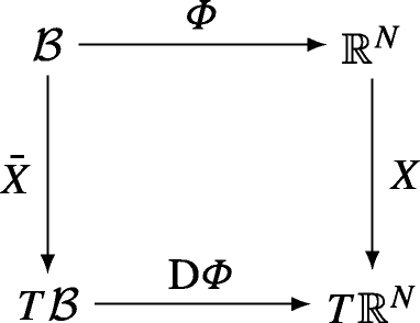
  In other words, $\bar X$ and X are related by the push-forward of $\bar X$ by Φ, that is ${{\varPhi }}_{*}(\bar X)=X$, in the sense $\text {D}{{\varPhi }}\circ \bar X=X\circ {{\varPhi }}$.⁵

• 3. Let $\mathcal {A}=\left \{ (K_{i},{{\varPhi }}_{i})\right \}$, with i = 1,…,M, be a smooth atlas of ${\mathscr{B}}$. This means that (K_i,Φ_i) is a chart of ${\mathscr{B}}$, the open sets K_i cover ${{\mathscr{B}}}$, and ${{\varPhi }}_{i}:K_{i}\subset {{\mathscr{B}}}\to {\mathbb {R}}^{N}$ is a diffeomorphism. Then, there are local vector fields $\bar X_{i}$ defined on K_i and given by $\bar X_{i}={\text {D}} {{\varPhi }}_{i}^{-1}\circ X\circ {{\varPhi }}_{i}$.

• 4. On each chart K_i, let us introduce a local controller $\bar u_{i}$, and define as $\bar X_{i}^{\text {cl}}:=\bar X_{i} + \bar u_{i}$ the local closed-loop vector field. Naturally, $\bar u_{i}$ is a local vector field on K_i.

• 5. Let $\bar \psi _{i}:K_{i}\to \mathbb {R}$ be a bump function with compact support $\bar {\mathcal {N}}_{i}\subset K_{i}$. We choose each $\bar {\mathcal {N}}_{i}$ such that if K_i ∩ K_j≠∅ then $\bar {\mathcal {N}}_{i}\cap \bar {\mathcal {N}}_{j}\neq \emptyset$ as well. Note that

  $$ \bar\varphi_{i}:=\frac{\bar\psi_{i}}{{\sum}_{i=1}^{M}\bar\psi_{i}} $$

  (91)

  is a partition of unity subordinate to the open cover $\left \{ K_{i}\right \}_{i=1}^{M}$.

• 6. The sum

  $$ \bar u:={\sum}_{1=1}^{M} \bar\varphi_{i} \bar u_{i} $$

  (92)

  is, by virtue of the partition of unity, well defined as a global controller on ${\mathscr{B}}$. Therefore, the global closed-loop vector field $\bar X^{\text {cl}}:=\bar X+\bar u$ is also well defined.

• 7. Let us now blow-down $\bar X^{\text {cl}}$. To be more precise, we now define the closed-loop vector field X^cl on $\mathbb {R}^{N}$ by ${{\varPhi }}_{*}(\bar X^{\text {cl}})=X^{\text {cl}}$. So, we have

  $$ X^{\text{cl}} = {{\varPhi}}_{*}(\bar X^{\text{cl}}) = {{\varPhi}}_{*}(\bar X+\bar u ) = {{\varPhi}}_{*}(\bar X) + {{\varPhi}}_{*}(\bar u)=X+ {{\varPhi}}_{*}(\bar u), $$

  (93)

  where we have used the fact that the push-forward is linear [45]. Next we define $u:={{\varPhi }}_{*}(\bar u)$ and compute

  $$ \begin{array}{ll} u={{\varPhi}}_{*}(\bar u) ={{\varPhi}}_{*}\left( {\sum}_{i=1}^{M}\bar\varphi_{i}\bar u_{i} \right)={\sum}_{i=1}^{M}{{\varPhi}}_{*}(\bar\varphi_{i}\bar u_{i})={\sum}_{i=1}^{M}({{\varPhi}}_{i})_{*}(\bar\varphi_{i}\bar u_{i})\\ ~~~~~~~~~~~~~~~~~={\sum}_{i=1}^{M} \varphi_{i}\cdot({{\varPhi}}_{i})_{*}(\bar u_{i}), \end{array} $$

  (94)

  where $\varphi _{i}:=\bar \varphi _{i}\circ {{\varPhi }}_{i}^{-1}$ for i = 1,…,M, and it is clear from its definition that $\left \{ \varphi _{i} \right \}$ is a partition of unity a neighborhood of the origin $0\in \mathbb {R}^{N}$ subordinate to the open cover $\left \{ {{\varPhi }}_{i}(K_{i}) \right \}$.

With the previous methodology, we define the controller that stabilizes canard cycles of the van der Pol oscillator as

$$ u=\frac{1}{2}\psi_{1}u_{1}+\frac{1}{2}\psi_{2}u_{2}, $$

(95)

where u₁ is as given by Lemma 4 and u₂ as in Theorem 1, and where ψ₁ is a bump function with support $\mathcal {N}_{1}$ containing the repelling branch ${\mathcal {S}}_{0}^{{\text {r}}}$ and ${\mathcal {N}}_{2}$ the parabola $\left \{ y=x^{2} \right \}$ around the origin. Although several choices for these neighbourhoods are possible, we recall an example given at the beginning of Section 4:

$$ \begin{array}{ll} \mathcal{N}_{1} = \left\{ (x,y)\in\mathbb{R}^{2} : |-y+x^{2}-\frac{1}{3}x^{3}|<\beta_{1}, 0<x<2, y_{\text{min}}<y<y_{h} \right\}\\ \mathcal{N}_{2} = \left\{ (x,y)\in\mathbb{R}^{2} : |-y+x^{2}|<\beta_{2}, -x_{\text{min}}<x<x_{\text{max}} \right\}, \end{array} $$

(96)

with suitably chosen positive constants β₁, β₂, x_min, x_max, y_min, $y_{h}<\frac {4}{3}$. We note that one must choose $0<y_{\min \limits }\in {\mathcal {O}}({\varepsilon })$ in order to ensure that the slow manifold ${\mathcal {S}}_{{\varepsilon }}^{{\text {r}}}$ is within distance ${\mathcal {O}}({\varepsilon })$ of the critical manifold ${\mathcal {S}}_{0}^{{\text {r}}}$. Here, y_h controls the height of the desired canard cycle, therefore $y_{h}<\frac {4}{3}$. The neighborhood ${\mathcal {N}}_{1}$ and ${\mathcal {N}}_{2}$ are sketched in Fig. 7.

With the controller as in Eq. 95, and given the analysis in Section 4.1, one has that orbits of Eq. 58 passing close to the origin follow closely the repelling branch of the slow manifold ${\mathcal {S}}_{{\varepsilon }}^{{\text {r}}}$ up to a height determined by y_h. Once orbits leave the neighborhood ${\mathcal {N}}_{1}\cup {\mathcal {N}}_{2}$, they are governed by the open-loop dynamics. Finally, the controller of Proposition 2 is indeed Eq. 95. We have just dropped the subscript of the constant $x_{1}^{*}$.

5 Conclusions and Outlook

In this paper, we have presented a methodology combining the blow-up method with Lyapunov-based control techniques to design a controller that stabilizes canard cycles. The main idea is to use a first integral in the blow-up space to regulate the canard cycle that the orbits are to follow. Later on, we have extended the previously developed method to control canard cycles in the van der Pol oscillator. Roughly speaking, this procedure follows two steps: first one needs a controller that stabilizes a folded maximal canard within a small neighborhood of the canard point. Next, one needs to stabilize the unstable branch of the open-loop slow manifold and to tune the position of the closed-loop orbits with respect to it. This is essential to determine whether the closed-loop canard has a head or not. Finally, one combines such controllers by means of a partition of unity. We have further shown that the proposed controller can be used to produce stable MMOs.

Several new questions and possible extensions arise from our work, and we would like to finish this paper by briefly mentioning a couple of ideas. First of all, it becomes interesting to adapt the controllers designed here to neuron models such as the FitzHugh-Nagumo, Morris-Lecar, or Hodgkin-Huxley models. Another relevant extension is to develop optimal controllers to control canards. Although from a theoretical point of view one would be interested in arbitrary cost functionals, some particular choices might be more suitable for applications. For instance, one may one want to design minimal energy controllers. It is also not completely clear whether the strategy of combining the blow-up method and control techniques still applies as the optimal controllers may be time-dependent. Finally, the notion of controlling MMOs definitely requires further investigation, as here we have just given a simple sample of the possibilities. Thus, for example, extending the ideas of this paper to higher-dimensional fast-slow systems with non-hyperbolic points is a direction to be pursued in the future.

References

Arnol’d VI, Varchenko AN, Gusein-Zade SM. Singularities of differentiable maps: Volume I : Classification of critical points, caustics and wave fronts. Berlin: Springer Science & Business Media; 2012.
Artstein Z. Asymptotic stability of singularly perturbed differential equations. J Diff Equ 2017;262(3):1603–16.
Artstein Z. Invariance principle in the singular perturbations limit. Discrete Contin Dynam Syst - B 2019;24:3653.
Artstein Z, Gaitsgory V. Tracking fast trajectories along a slow dynamics: a singular perturbations approach. SIAM J Control Optim 1997;35(5):1487–1507.
Artstein Z, Leizarowitz A. Singularly perturbed control systems with one-dimensional fast dynamics. SIAM J Control Optim 2002;41(2):641–58.
Banasiak J, Lachowicz M. Methods of small parameter in mathematical biology. Berlin: Springer; 2014.
Benoît E. Chasse au canard. Collectanea Math 1981;31-32(1-3): 37–119.
Benoît E. Canards et enlacements. Publications Mathématiques de l’Institut des Hautes É,tudes Scientifiques 1990;72(1):63–91.
Brøns M, Bar-Eli K. Canard explosion and excitation in a model of the belousov-zhabotinskii reaction. J Phys Chem 1991;95(22):8706–13.
Chow JH, Peponides G, Kokotovic PV, Avramovic B, Winkelman JR, Vol. 46. Time-scale modeling of dynamic networks with applications to power systems. Berlin: Springer; 1982.
Coppel WA, Vol. 629. Dichotomies in stability theory. Berlin: Springer; 2006.
Desroches M, Guckenheimer J, Krauskopf B, Kuehn C, Osinga HM, Wechselberger M. Mixed-mode oscillations with multiple time scales. SIAM Rev 2012;54(2):211–88.
Dmitriev MG, Kurina GA. Singular perturbations in control problems. Autom Remote Control 2006;67(1):1–43.
Dorfler F, Bullo F. Synchronization and transient stability in power networks and nonuniform kuramoto oscillators. SIAM J Control Optim 2012;50(3): 1616–42.
Dumortier F, Roussarie R, Vol. 577. Canard cycles and center manifolds. Rhode Island: American Mathematical Society; 1996.
Durham J, Moehlis J. Feedback control of canards. Chaos Interdiscipl J Nonlin Sci 2008;18(1):015110.
Eckhaus W, Vol. 6. Matched asymptotic expansions and singular perturbations. Amsterdam: Elsevier; 2011.
Ermentrout GB, Terman DH, Vol. 35. Mathematical foundations of neuroscience. Berlin: Springer Science & Business Media; 2010.
Fenichel N. Persistence and smoothness of invariant manifolds for flows. Ind Univ Math J 1971;21(3):193–226.
Fenichel N. Geometric singular perturbation theory for ordinary differential equations. J Diff Equ 1979;31(1):53–98.
FitzHugh R. 1969. Mathematical models of excitation and propagation in nerve. Biol Eng 1–85.
Fridman E. A descriptor system approach to nonlinear singularly perturbed optimal control problem. Automatica 2001;37:543–49.
Fridman E. 2001. State-feedback h control of nonlinear singularly perturbed systems.
Hairer E, Wanner G, Vol. 14. Solving ordinary differential equations II: stiff and differential-algebraic problems. Berlin: Springer; 2010.
Hek G. Geometric singular perturbation theory in biological practice. J Math Biol 2010;60(3):347–86.
Izhikevich EM. Dynamical systems in neuroscience. Cambridge: MIT Press; 2007.
Jardon-Kojakhmetov H, Kuehn C. 2019. A survey on the blow-up method for fast-slow systems. arXiv:1901.014021901.01402.
Jardón-Kojakhmetov H, Muñoz-Arias M, Scherpen JMA. Model reduction of a flexible-joint robot: a port-hamiltonian approach. IFAC-PapersOnLine 2016;49(18):832–37.
Jardón-Kojakhmetov H, Scherpen JMA. Model order reduction and composite control for a class of slow-fast systems around a non-hyperbolic point. IEEE Control Syst Lett 2017;1(1):68–73.
Jardón-Kojakhmetov H., Scherpen JMA, del Puerto-Flores D. Stabilization of a class of slow–fast control systems at non-hyperbolic points. Automatica 2019;99:13–21.
Jones CKRT. Geometric singular perturbation theory. In: Dynamical systems. Berlin: Springer; 1995. p. 44–118.
Kaper HG, Kaper TJ, Zagaris A. Geometry of the computational singular perturbation method. Mathematical Modelling of Natural Phenomena 2015; 10(3):16–30.
Kaper TJ. An introduction to geometric methods and dynamical systems theory for singular perturbation problems. Analyzing multiscale phenomena using singular perturbation methods. American Mathematical Soc; 1999. p. 85–131.
Kevorkian JK, Cole JD, Vol. 114. Multiple scale and singular perturbation methods. Berlin: Springer Science & Business Media; 2012.
Kokotović P., Khalil HK, O’Reilly J. 1999. Singular perturbation methods in control: analysis and design, vol. 25 SIAM.
Kokotović PV. Applications of singular perturbation techniques to control problems. SIAM Rev 1984;26(4):501–50.
Kokotović PV, Allemong JJ, Winkelman JR, Chow JH. Singular perturbation and iterative separation of time scales. Automatica 1980;16(1): 23–33.
Kokotović PV, O’Malley RE Jr, Sannuti P. Singular perturbations and order reduction in control theory—an overview. Automatica 1976;12(2): 123–32.
Krupa M, Szmolyan P. Extending geometric singular perturbation theory to nonhyperbolic points—fold and canard points in two dimensions. SIAM J Math Anal 2001;33(2):286–314.
Krupa M, Szmolyan P. Relaxation oscillation and canard explosion. J Diff Equ 2001;174(2):312–68.
Kuehn C, Vol. 191. Multiple time scale dynamics. Berlin: Springer; 2015.
Kunkel P, Mehrmann V, Vol. 2. Differential-algebraic equations: analysis and numerical solution. Europe: European Mathematical Society; 2006.
Kurina GA, Dmitriev MG, Naidu DS. Discrete singularly perturbed control problems (a survey). Dynamics of Continuous. Discrete Impuls Syst Series B Appl Algo 2017;24(5):335–70.
LaSalle J. Some extensions of Liapunov’s second method. IRE Trans Circ Theor 1960;7(4):520–27.
Lee JM. Smooth manifolds. Introduction to smooth manifolds. Berlin: Springer; 2013. p. 1–31.
Mishchenko EF, Rozov NK. Differential equations with small parameters and relaxation oscillations. Berlin: Springer; 1980.
Moehlis J. Canards in a surface oxidation reaction. J Nonlin Sci 2002; 12(4):319–45.
Nagumo J, Arimoto S, Yoshizawa S. An active pulse transmission line simulating nerve axon. Proc IRE 1962;50(10):2061–70.
Naidu DS. Singular perturbations and time scales in control theory and applications: an overview. Dynam Cont Discrete Impuls Syst Ser B 2002;9:233–78.
Naidu DS, Calise AJ. Singular perturbations and time scales in guidance and control of aerospace systems: A survey. J Guid Control Dynam 2001;24(6): 1057–78.
O’Malley RE Jr. Singular perturbation methods for ordinary differential equations, volume 89 of Applied Mathematical Sciences. New York: Springer; 1991.
Sanders JA, Verhulst F, Murdock JA, Vol. 59. Averaging methods in nonlinear dynamical systems. Berlin: Springer; 2007.
Siciliano B, Book WJ. A singular perturbation approach to control of lightweight flexible manipulators. Int Robot Res 1988;7(4):79–90.
Spong MW. 1990. Control of flexible joint robots: a survey. Coordinated Science Laboratory Report no. UILU-ENG-90-2203 DC-116.
Takens F. Constrained equations; a study of implicit differential equations and their discontinuous solutions. Structural stability, the theory of catastrophes, and applications in the sciences. Springer; 1976. p. 143–234.
Verhulst F, Vol. 50. Methods and applications of singular perturbations: boundary layers and multiple timescale dynamics. Berlin: Springer Science & Business Media; 2005.
Wechselberger M. A propos de canards. Trans Am Math Soc 2012; 364(6):3289–09.
Funding
Open access funding provided by the University of Groningen. HJK gratefully acknowledges support by a fellowship of the Alexander-von-Humboldt Foundation. CK acknowledges partial support by the DFG via the SFB/TR109 Discretization in Geometry and Dynamics and support by a Lichtenberg Professorship of the VolkswagenFoundation.
Author information
Authors and Affiliations
Corresponding author
Additional information
Publisher’s Note
Springer Nature remains neutral with regard to jurisdictional claims in published maps and institutional affiliations.
Rights and permissions
Open Access This article is licensed under a Creative Commons Attribution 4.0 International License, which permits use, sharing, adaptation, distribution and reproduction in any medium or format, as long as you give appropriate credit to the original author(s) and the source, provide a link to the Creative Commons licence, and indicate if changes were made. The images or other third party material in this article are included in the article's Creative Commons licence, unless indicated otherwise in a credit line to the material. If material is not included in the article's Creative Commons licence and your intended use is not permitted by statutory regulation or exceeds the permitted use, you will need to obtain permission directly from the copyright holder. To view a copy of this licence, visit http://creativecommons.org/licenses/by/4.0/.
About this article
Cite this article
Jardón-Kojakhmetov, H., Kuehn, C. Controlling Canard Cycles. J Dyn Control Syst 28, 517–544 (2022). https://doi.org/10.1007/s10883-021-09553-2
Received:
Revised:
Accepted:
Published:
Issue Date:
DOI: https://doi.org/10.1007/s10883-021-09553-2