
Abstract
Elastic contact between a non-ideal Berkovich indenter and a half-space is investigated. The derived mathematical model of the contact allows for tangential displacements of the boundary points of the half-space. The tip of the blunted indenter is simulated as a smooth surface. The boundary element method is implemented in the model for numerical simulation of nanoindentation. The relative deviation function is introduced and calculated to quantify the influence of the tangential displacements on the load–displacement curves. A simple expression is derived for the impact of the tangential displacements on the values of the reduced Young’s modulus determined due to nanoindentation studies. The refined model was successfully applied to simulate the experimental load–displacement curves gained by elastic nanoindentations of flat LiF and KCl samples. Such values of the indenter bluntness (the varying parameter) were found that the simulated load–displacement curves coincided with those of the experimental data at displacements higher than 7.5 nm. The model neglecting tangential displacements gives slightly differing values for the parameter of the indenter bluntness.


Abbreviations
- O, x1, x2, x3 :
-
Cartesian coordinate system
- M, N :
-
Points on the plane x3 = 0
- R MN :
-
Distance between points M(x1, x2) and N(ξ, η)
- r :
-
Distance between point M and the origin O, \( r = \sqrt {x_{1}^{2} + x_{2}^{2} } \)
- h :
-
Displacement of the indenter
- f(x1, x2):
-
Gap between the indenter and the specimen before deformation
- γ:
-
Angle between Ox3 and O′E, depends on the position of M (see Fig. 1)
Fig. 1 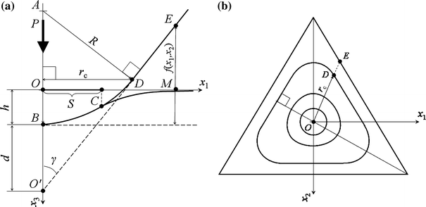
a Geometry of the simulated blunted indenter, BCDE, and of the ideal Berkovich indenter, O′DE. The segment BD is the arc of the circle with the centre A and radius R; d is the bluntness of the indenter tip. OB is the displacement of the indenter, which causes the contact BC with the sample. b Cross-section of the simulated blunted indenter. The contour lines correspond to various positions of D
- R :
-
Radius describing the shape of the blunted indenter tip, depends on the position of M
- β:
-
Indenter parameter, β = cot 65.3° = 0.46
- d :
-
Bluntness of the indenter tip
- r c :
-
Distance between the origin O and the contour of the orthogonal projection of the bluntness to the plane x3 = 0
- S :
-
Orthogonal projection of the contact region on the plane x3 = 0 after deformation
- Ω:
-
An arbitrary area in the plane x3 = 0 containing the contact region
- \( v(M),\;M \in \Upomega \) :
-
Unknown function in the integral boundary equation
- P :
-
Force applied to the indenter in the direction normal to the flat surface of the specimen
- P0(h):
-
Dimensionless compression force
- \( E_{\text{i}} ,\;\upsilon_{\text{i}} \) :
-
Young’s modulus and Poisson’s ratio respectively of the diamond indenter
- \( E_{\text{s}} ,\;\upsilon_{\text{s}} \) :
-
Young’s modulus and Poisson’s ratio respectively of the sample
- K(M, N):
-
Kernel of the integral operator
- ε:
-
\( \varepsilon = \frac{1}{2} \cdot \frac{{1 - 2\upsilon_{s} }}{{1 - \upsilon_{s} }} \)

References
Hertz H (1882) J Reine Angew Math 92:156
Galanov BA (1982) Dokl Akad Nauk Ukr SSR 7:36
Galanov BA, Grigor’ev ON (1986) Strength Mater 18:1330
Brock LM (1979) Int J Eng Sci 17:365
Georgiadis HG (1998) Comput Mech 21:347
Soldatenkov IA (1994) Mekh Tverd Tela 4:51
Soldatenkov IA (1996) J Appl Math Mech 60:261
Galanov BA (1983) Mekh Tverd Tela 6:56
Argatov II (2004) J Appl Mech Tech Phys 45:118
Argatov II (2004) Dokl Phys 49:222
Herrmann K, Jennett NM, Wegener W et al (2000) Thin Solid Films 377:394
Borodich FM, Keer LM, Korach CS (2003) Nanotechnology 14:803
Galanov BA (1993) J Math Sci 66:2414
Galanov BA (1985) J Appl Math Mech 49:634
Borodich FM, Keer LM (2004) Int J Solids Struct 41:2479
Kindrachuk VM, Galanov BA, Kartuzov VV et al (2006) Nanotechnology 17:1104
Johnson KL (1985) Contact mechanics. Cambridge University Press, Cambridge
Vlassak JJ, Nix WD (1994) J Mech Phys Solids 42:1223
Vlassak JJ, Ciavarella M, Barber JR et al (2003) J Mech Phys Solids 51:1701
Pharr GM, Oliver WC, Brotzen FR (1992) J Mater Res 7:613
Mencik J (2007) Meccanica 42:19
Oliver WC, Pharr GM (2004) J Mater Res 19:3
Khan MK, Hainsworth SV, Fitzpatrick ME et al (2009) J Mater Sci 44:1006. doi:https://doi.org/10.1007/s10853-008-3222-9
Landau LD, Lifshitz EM (1986) Theory of elasticity. Pergamon Press, New York
Author information
Authors and Affiliations
Corresponding author
Appendices
Appendix A
Accordingly to [8] the nonlinear boundary integral equation of the contact problem accounting for tangential displacements is:
Here u(M) and w(M) are the tangential displacements in point M in the directions Ox1 and Ox2 respectively, v +(M) is the contact pressure. We assume that these displacements are small compared to the dimensions of the contact region. In this case the function \( f(x_{1} + u(M),\,x_{2} + w(M)) \) from Eq. 13 can be approximated by:
where f(M) is defined in (5). We denote further R(M) as R.
The tangential displacements induced by the surface of the bluntness can be introduced as [24]:
Therefore,
and Eq (13) allowing for the tangential displacements can be written as
In the present formulation of the contact problem the magnitude of the radius R depends on the position of the point M.
Appendix B
Let us formulate the problem (2) in a dimensionless coordinate system \( x_{\text{i}} = \sqrt {2hd} x_{{0{\text{i}}}} \) and also introduce the dimensionless unknown function \( U(x_{01} ,x_{02} ) = \lambda \cdot \sqrt {{{2d} \mathord{\left/ {\vphantom {{2d} h}} \right. \kern-\nulldelimiterspace} h}} \cdot v(x_{1} ,x_{2} ). \) We then write the NBIEs (2) in the following dimensionless form:
where M0 and N0 are the points on the plane x03 = 0 with the coordinates (x01, x02) and \( (\xi_{0} ,\eta_{0} ) \) respectively. P0(h) is the dimensionless compression force. The square \( \Upomega_{0} = \left\{ {M_{0}{:}\;\left| {x_{01} } \right| \le 6,\;\left| {x_{02} } \right| \le 6} \right\} \) is an image of the square Ω after changing variables. The value 6 is chosen in order that the square Ω0 includes the contact region \( S_{0} = \left\{ {M_{0} :\;U(M_{0} ) \ge 0} \right\} \subseteq \Upomega_{0} . \) Similarly, the dimensionless tangential displacements are given by:
The final formula for constructing the P(h) diagram for the approach of the indenter and the sample can be obtained by substituting the second equation in (15) into the second equation in (2)
The collocation method is used for the discretization of (15). The integrals are approximated by the rectangle formula. To solve the discretized equation the generalized Newton’s method is applied.
The region Ω0 is divided into 1024 equal pieces (i.e. 1089 nodes). Numerical simulations show that the generalized Newton’s method converges to the exact solution of the discretized form of the first equation in (15) usually after five iterations at the discrepancy for each node of 1 × 10⁻⁵.
Before starting the numerical simulations, the solution of the NBIEs (15) was compared with that one of the Hertzian problem. For this purpose we assume \( s(x_{1} ,x_{2} ) = {\text{const}} = 1 \) and υs = 0.5. In this case:
holds for the compressive force P (see (17)). The solution of the dimensionless NBIEs (15) yields \( P_{0} (h) = {\text{const}} = 0.3 \pm 2 \cdot 10^{ - 4} . \) Let us compare with the Hertzian problem [17, 24]:
where \( \frac{2\sqrt 2 }{3\pi } \approx 0.30011. \)
Rights and permissions
About this article
Cite this article
Kindrachuk, V.M., Galanov, B.A., Kartuzov, V.V. et al. Refined model of elastic nanoindentation of a half-space by the blunted Berkovich indenter accounting for tangential displacements on the contact surface. J Mater Sci 44, 2599–2609 (2009). https://doi.org/10.1007/s10853-009-3340-z
Received:
Accepted:
Published:
Issue Date:
DOI: https://doi.org/10.1007/s10853-009-3340-z