A component-based design approach for energy flexibility in cyber-physical manufacturing systems

Abstract

Energy flexibility of manufacturing systems helps to meet sustainable manufacturing requirements and is getting significant importance with rising energy prices and noticeable climate changes. Considering the need to proactively enable energy flexibility in modern manufacturing systems, this work presents a component-based design approach that aims to embed energy flexibility in the design of cyber-physical production systems. To this end, energy management using Industry 4.0 technologies (e.g., Internet of Things and Cyber-physical Systems) is compared to the literature on energy flexibility in order to evaluate to what extent the energy flexibility practice takes advantage of Industry 4.0 technologies. Another dimension is the coverage of the life cycle of the manufacturing system which guarantees its sustainable design and the ability to achieve energy flexibility by configuring the energy consumption behaviour. A data-based design approach of the energy-flexible components is proposed in the spirit of the Reference Architectural Model Industrie 4.0 (RAMI 4.0), and then it is exemplified using an electric drive (as a component) in order to show the practical applicability of the approach. The energy consumption behaviour of the component is modelled using machine learning techniques. The digital twin of the studied component is developed using Visual Components virtual engineering environment, then its energy consumption behaviour is included in the model allowing the system integrator/decision-maker to configure the component based on the energy availability/price. Finally, external services in terms of an optimisation module and a deep learning module are connected to the digital twin.

Introduction

Fig. 1

The components development position in the manufacturing system life cycle (Based on (Konstantinov et al., 2022))

The United Nations Organisation (UN) issued in 2015 an agenda titled “Transforming our world: the 2030 Agenda for Sustainable Development” which determined the Sustainable Development Goals. Among these goals are: “affordable and clean energy” (goal 7) (UN, 2015a), “industry innovation and infrastructure” (goal 9) (UN, 2015b). The former targets to double the improvement of energy efficiency by 2030, and the latter aims to upgrade industries so that they become sustainable in terms of increased resource-use efficiency and environmentally sound technologies and industrial processes. On the customers’ side, there is a trending lifestyle that is oriented towards care for the environment as a result of the awareness of the scarcity of resources, and many companies are adopting the concept of cleaner production to satisfy customer demands (Hojnik et al., 2019). In addition, In the same vein, it has been reported that customer behaviour is changing from being price-sensitive to being carbon emission-sensitive (Jiang & Chen, 2016).

Although the use of renewable energy is becoming a “green solution” for decarbonised power supply, it presents challenges on both the supply and demand sides. On the supply side (the grid), the dynamics, control and automation of power systems constitute a real challenge due to the volatility and variability of power generation by renewable plants (Sajadi et al., 2018). Regarding the demand side, it is widely recognised that production rates respond to market requirements, which are inherently unstable and influenced by many variables.

The concept of energy flexibility (EF) has gained increased importance due to the growing reliance on renewable energy resources. In production systems, it is defined as “the capability to react quickly and cost-efficiently to alternating energy availability” (Popp et al., 2017; Graßl et al., 2014). On the organisational level, energy flexibility can be understood as the ability to schedule manufacturing processes depending on the energy features (Popp et al., 2017). Technically, at the component level, prioritising energy availability in the real-time adaption of the energy demand can be expressed in terms of its energy flexibility (Popp et al., 2017).

The emerge of the Fourth Industrial Revolution holds great potential for sustainable manufacturing and promises to improve the sustainable use of resources. In the body of this work, the Internet of Things (IoT), cloud computing, and Cyber-Physical Systems (CPS) are considered as Industry 4.0 technologies. Thanks to IoT technologies and cloud computing, monitoring of global $\hbox {CO}_2$ emissions is possible, and many major economies (e.g., China, UK and Germany) can achieve their sustainable energy use targets. Although this thinking model has not fully permeated, some early implementations provide a glimpse of the expected outcomes.

Therefore, considering the freshness and the necessity of the energy flexibility concept, this work aims to embed energy flexibility in the design of cyber-physical production systems (CPPS). In particular, from a manufacturing system life cycle perspective (Fig. 1), the focus is on the design of the “components” that will collectively form the manufacturing cells. An Industry 4.0-inspired design approach is constructed, and Industry 4.0 technologies are harnessed.

The remainder of this paper is as follows: Sect. “Literature review” reviews the literature related to the energy flexibility of manufacturing and the support of Industry 4.0 to energy management. Sect. “A component-based approach for embedding energy flexibility” presents the methodology proposed to support the foundation of the intended design approach. A case study is exemplified in Sect. “An Empirical evaluation of the proposed approach” to clarify the possible implementation means, followed by a discussion in Sect. “Discussion”. Finally, Sect. “Conclusion and future work” concludes the paper.

Literature review

The following literature review aims, first and for most, at investigating the recent energy management practices inspired by Industry 4.0, and, subsequently, the status of the energy flexibility of manufacturing systems. Next, the research gap is analysed, and research questions are derived.

Energy management under Industry 4.0

Tao et al. (2014) put forward a method for energy saving and emission reduction based on IoT and Bill of Material (BoM). In this method, the concept of Big BoM combines the data existing in each stage, the related energy consumption, the environmental impact, in addition to the basic data. Big BoM relies heavily on big data and IoT to be established. Wang et al. (2016) present an IoT-based product life cycle energy management (PLEM). In their proposal, in the ‘production’ phase of the product life cycle, they highlight the fact that IoT may help to reduce idle time and define energy consumption as a function of a certain configuration. Through interviews with some technology/solution providers, Shrouf and Miragliotta (2015) attempted to show the influence of IoT on energy management in manufacturing. As a result, it is shown that IoT-enabled solutions can support various functions of energy efficiency and production management decision-making.

To monitor and manage machine tool energy consumption, Chen et al. (2018) believe that there are two approaches: monitoring the process route including cutting parameters, and benchmarking the energy consumption of the machining task to decrease standby energy consumption. As a result, the implemented IoT-based system could switch off unnecessary machine tools and choose energy-efficient machining routes by comparing the records. At the production planning and control level, particularly scheduling, Wang et al. (2018) aim to optimise real-time energy efficiency by adopting IoT technology. To achieve this, production planning relies on the data obtained from the shop floor. Thus, a scheduling/rescheduling plan is created based on energy data. Pelzer et al. (2016) developed a ‘cross energy data model’ as a part of an energy management system. The model objects include classes that describe the properties of power storage, power plants, manufacturing processes, and their scheduling. Foumani and Smith-Miles (2019) believe that responding to the carbon reduction policies implies the improvement of green flowshop scheduling models. Additionally, they take into account the involvement of sustainability managers by offering them a tool that realises both the sustainability and productivity of the operations. Touching on the productivity and profitability under government carbon tax and carbon quota policies as well, Zhu et al. (2023) identify three green manufacturing modes that the manufacturer should be able to switch between so that more profit is acquired.

Looking at the use of CPS and digital twin (DT) for the shop-floor, Zhang et al. (2020) include energy consumption rules in the behavioural description of the shop-floor DT. In pursuit of dynamically scheduling the production on a machine tool shop floor, Feng et al. (2018) established a Wireless Sensor Network (WSN) to collect data, then a tool aging model is built and utilised together with the geometry information to schedule the production and increase the energy efficiency. A Genetic Algorithm is used to optimise manufacturing energy consumption. Max-plus Algebra is used by Wang et al. (2019) to make decisions about machine states (active/idle) after incorporating it as a service in the digital space. In this approach, the DT has an event-driven energy-saving decision model which outputs the suitable decision relying on the data received from the physical system. A cyber-physical toolset for plant energy prediction and optimisation is introduced by Pease et al. (2018). The developed toolset could monitor, predict and control the power consumption of a CNC machine for different processes. To overcome the heterogeneity of the involved devices, a variety of IoT protocols were used in a four-layer architecture. Pei et al. (2018) explored the “elastic” segments of energy production, conversion and consumption, then modelled them in a mathematical model in order to ensure the fulfilment of production tasks under economic and energy constraints. The application is exemplified in a lithium battery manufacturing plant in cyber-physical environments.

The control systems’ view of the production facility decomposes it into hierarchical levels. The interactions between the elements of a certain level impact those at the higher level, including, their energy consumption Diaz C. and Ocampo-Martinez (2019). Targeting energy efficiency improvement implies possessing sufficient knowledge of every level, its elements and the possible interactions. Focusing on the machine process level, Mawson and Hughes (2019) utilised the Discrete Event Simulation (DES) with the collected energy data to improve the system’s energy consumption performance.

Referring to digital twin-driven product design, Tao et al. (2018) believe that following such an approach increases efficiency, sustainability and the design of the product, its manufacturing and service. A web-based platform for knowledge sharing is introduced by Kannan and Arunachalam (2019), where a digital twin for the grinding wheel is created. By using a DT, energy consumption could be reduced by 14.4% compared to the conventional methods. Rocca et al. (2020) consider that digital technologies can support the circular economy at the factory level. Therefore, they developed an energy management application for disassembly processes. This application monitors an energy consumption indicator by means of the disassembly’s DT.

A framework for data-driven sustainable intelligent manufacturing based on demand response (DR) for energy-intensive industries is proposed by Ma et al. (2020). On a cloud platform, a variety of applications are built including an energy monitoring application, a parameter optimisation application, and an energy warning application. Katchasuwanmanee et al. (2016) constructed an architecture of an energy-smart production management system. Big data used here include weather forecasts, production schedules and machines’ energy consumption. Consequently, correlation analysis is created by understanding the relationship between energy flow and workflow. Zhang et al. (2020) develop a method to detect hybrid data association (i.e., production data and energy consumption). Also, a big data-driven analysis is conducted by means of Deep Belief Networks in order to detect production anomalies. Neural Networks were used by Yu et al. (2017) to search for power-saving opportunities by analysing big data associated with semiconductor production. By identifying the relationship between the input parameters and the power consumption per toolset move, the best setup can be chosen.

Energy flexibility in manufacturing

Roth et al. (2021) seek to optimise the difference between the cost of energy bought from the grid and the energy fed by the energy storage system. The implementation of this approach took place at a medium-sized company that has photovoltaics for energy generation and production processes whose loads can be shifted. System parameters (e.g., buffer capacity and system utilisation) in addition to scheduling the processes are proposed by Beier et al. (2017). The aim here is to maintain the production system throughput while receiving electrical energy feed from on-site variable renewable energy (VRE) sources. In the food industry and under the smart manufacturing theme, Angizeh et al. (2020) developed an optimisation model that harmonises the optimal assignments of product and labour with the production line schedule under the constraints of electricity prices and product demand. Further, a sensitivity analysis is performed to understand the effect of various scenarios on the optimal targets. Also in Angizeh and Parvania (2019), a two-stage optimisation model is introduced where, an objective function based on electricity cost is optimised taking into account the uncertainty of solar energy. In the first stage, this considers flexible load rescheduling along with energy storage and on-site solar generation. In the second stage, the decision of whether to purchase energy or to sell the extra is made.

In machine tools, Popp et al. (2017) evaluated the potential of energy demand reduction in energy-flexible machine tool components, with the aim of maintaining productivity while balancing the residual loads. Materi et al. Materi et al. (2020) discussed the influence of supply energy on the machine tool operation parameters e.g., cutting speed. Thus, they built a numerical model to correlate productivity (represented by cutting speed) with the available energy obtained from renewables. The demand is calculated from a discrete uniform distribution, and the buffer is the remainder from the previous day. For other types of machines (e.g., thermoforming), Brugger et al. (2017) propose to analyse the process step and rely on the control programme to analyse energy-flexible process steps. Besides, a forecast model of each component is necessary to optimally use energy flexibility options. Although significant effort is put into using scheduling techniques to improve energy sustainability, neither an indication of the corresponding control is made, nor an explanation of the expected approach is provided. Regarding control particularly, Ivanov et al. (2021) state that currently, the way control methods can be applied to formulate scheduling accurately is not clear enough. As a result, the same problem can be expected to happen when scheduling manufacturing activities for increased energy flexibility.

Aiming to integrate energy flexibility in manufacturing system and product life cycles, Rödger et al. (2020) consider that manufacturing simulation can cover both, therefore, the processes’ energy demand is modelled by means of their states (e.g., on, off), where energy consumption is either fixed or variable. To validate this approach, 14 scenarios that include energy feed from volatile sources were tested. An IT platform to support the synchronisation between the company side and the market is introduced by Bauer et al. (2017). The proposed architecture relies on a Service-Oriented Architecture and provides Life Cycle management as one of the base services. Although a variety of simulation methods have been attempted to integrate energy flexibility in manufacturing systems, no solution to be classified as ‘universal’ exists (Köberlein et al., 2022).

Research gaps analysis

Looking at energy as a resource, it can be managed similar to other manufacturing resources (e.g., materials). In principle, all the approaches that are valid for energy management can be harnessed for further application of energy flexibility. As shown earlier, energy management under Industry 4.0 relied significantly on Cyber-Physical Systems, IoT, and Big Data technologies. On the other hand, the research on the energy flexibility of manufacturing systems covered various aspects such as scheduling, production planning and control and technical building services. The involvement of digital technologies is still limited, and their full advantage is not fully harnessed. DT, as a major component of the CPS, has been efficiently utilised for energy management under Industry 4.0, with the possibility of establishing connectivity to the web. However, its utilisation for improving energy flexibility is still poor.

A significant part of the aforementioned energy flexibility research approaches utilised production buffers and manipulated their capacity. In a typical discrete manufacturing industrial scenario, this is enabled by varying the processes’ time and speed. Thus, certain “influential” machine component settings are changed. If such changes are to take place in the hardware, they will take considerable time. In addition, the new settings era is supposed to be valid for a reasonable period of time. For software changes, the effect relies on the control programme structure and its built-in capabilities to be flexible enough. As a result, the planned changes should target the software side and the system should be designed to adapt to such changes. Energy flexibility literature did not exhibit any of the aforementioned approaches, rather, it still suffers scattering in terms of being case-specific and in the early phase, laying out its theoretical foundation. In addition, the reviewed literature exhibits a strong emphasis on the relationship between energy management and life cycle management towards more sustainable manufacturing, in general. As the manufacturing system should actively respond to external changes, taking into account energy flexibility, a proactive approach to enabling such a capability has to be constructed.

Following the arguments above, it becomes logical to search for the most suitable “building unit” that enables the system to interact positively with changes. On one hand, this requires understanding the behaviour of the building unit through energy consumption modelling in order to guarantee that energy flexibility management can be achieved across life cycle stages. In other words, there should be a system engineering approach in which the prototyping of energy flexibility is tested during the design phase. Thus, the main research questions to be investigated in this work are:

• $RQ_1$ How to proactively include energy flexibility starting from the design phase?

• $RQ_2$ What is the design approach to be considered when building an energy-flexible manufacturing system taking into account its life cycle, and in accordance with Industry 4.0?

A component-based approach for embedding energy flexibility

Design perspectives of building modern manufacturing systems

The emerge of Industry 4.0 gave sustainable manufacturing new horizons into creating innovative methods of adding value sustainably. As explained by Stock and Seliger (2016), the ‘Smart Factory’ will be transformed into an energy supplier in addition to being an energy consumer at the same time. Thus, supported by the smart grid, its energy management system should be capable of managing such resultant energy dynamics. Simultaneously, the embedded CPS will be customised to control value creation factors. The term “Energy Management 4.0” is coming to life now, and is a subject of continuous improvement and innovation by investigating the very fine granularity of energy data (Nienke et al., 2017).

There is no unified approach/methodology for building modern manufacturing systems in general, and those that consider the sustainability of energy particularly. For example, Medojevic et al. (2018) consider that there are two prominent types of approaches: model-based approaches and data-driven approaches. Model-based approaches can be very accurate and flexible when configuring input data, however, the non-linearity and stochastic characteristics of industrial systems may complicate building those models. For data-driven approaches, they rely on understanding the trends of behaviour by means of various methods such as regression analysis and neural networks. In this vein, IoT solutions support data-driven approaches by monitoring real-time system conditions. On the other hand, according to Saldivar et al. (2015), two technologies are realised when aiming at fostering the productivity of CPS: component-based design and model-based design, where CPS supports the capabilities of virtualisation, interoperability and decentralisation. In a model and component-based design flow, the starting point for building a system’s model is component models with the guidance of architectural specifications that include system scope, content, and composition (Harrison et al., 2016).

In this paper, looking analytically at the manufacturing systems, it is continuously perceived and broken down into smaller units. The better these units are defined in terms of their properties descriptions, the easier it is for systems designers/integrators to configure/reconfigure the system in general, and its sustainability performance, in particular. Digital representations in the Industry 4.0 era are used to collect and analyse data supporting the process of monitoring and reporting performance. Transferring from this ‘analytical’ understanding to a ‘synthetic’ one, where the focus is on the life cycle of the system, unless energy consumption properties are not stored in the digital representation of the system, harnessing its energy flexibility potential would not reach its maximum. Therefore, building an energy-flexible system requires the definition of the following aspects:

• The component: as a unit/entity to be used for building the system, which consumes energy and can be controlled.

• The digital representation: a transferrable digital asset that can be utilised by systems designers/integrators.

• The life cycle of the system: in terms of the phases in which the system’s behaviour is to be monitored so that the required standards of productivity and sustainability are adhered to.

• A method for embedding energy flexibility that results in an interaction with the digital representation in terms of controlling the parameters that affect energy consumption across the life cycle phases.

Component-based design using virtual engineering

A component is “an autonomous unit consisting of the automation device (i.e., actuator, sensor) with its own computing hardware (processor, memory, communication interface electronic interface to the automation device) and control software (application programmes, operating system and communication protocol) (Lee et al., 2004). Alkan and Harrison (2019) define component-based automation system (CBAD) as a “constellation of basic components which can be represented in various design domains, such as mechanical, electrical, pneumatic, control, etc.”. Under Industry 4.0, an “Industry 4.0 component” is a “worldwide identifiable participant able to communicate consisting of Asset Administration Shell (AAS) and Asset including a digital connection” (Wagner et al., 2017). AAS is a “virtual digital and active representation of an Industry 4.0 Component in an Industry 4.0 System” (Wagner et al., 2017). In other words, AAS is the logical unit responsible for the virtual representation, the interaction with the system and resource management (Moghaddam et al., 2018). As a result, the essential characteristic of the Industry 4.0 component is the combination of both physical and virtual worlds with the aim of providing certain functionalities within them. Figure 2 shows an example of the possible representations an AAS may contain.

Fig. 2

Asset Administration Shell (AAS) of an Industry 4.0 Component (image credit: ZVEI)

The life cycle of manufacturing systems goes through the following stages (Assad et al., 2021; Schneider et al., 2019):

• Engineering Requirements: The goal(s) of building the manufacturing system and functionalities intended by creating it.

• Specification: Defining the stages of production, and manufacturing processes by which sustainable value creation takes place.

• Physical build: The physical build of the system’s units and subsystems.

• Commissioning: Interfacing and integrating the subsystems and establishing the data communication channels.

• Operation and maintenance: Running the system and identifying faulty components and inefficient processes.

While going through the early design phases (prior to the operation), it is aimed to embed energy flexibility in the design of the components in the form of their virtual models, which eventually evolve into digital twins and constitute the cyber element of the CPS. As shown in Assad et al. (2021), virtual engineering tools can provide crucial support to sustainability in terms of reusing virtual models and reducing the time needed to reconfigure/redesign them. In addition to the aforementioned benefits, energy flexibility can be added in the design phase (or the early phases) at the component level to contribute to the system’s ability to respond to the change in energy demand.

The design of energy-flexible components

For manufacturing systems builders, there are numerous functions to be verified while building the system. Current simulation tools typically allow the creation of separate models of the system’s /process’s control logic, structure, etc. The ideal representation of all these functions can be obtained by building the digital twin. According to the Industrial Internet Consortium (IIC), the digital twin is “Information that represents attributes and behaviours of an entity”. In other words, “a formal digital representation of an entity, with attributes and optionally computational, geometrical, visualisation and other models, offering a service interface for interacting with it, adequate for communication, storage, interpretation, process and analysis of data pertaining to the entity in order to monitor and predict its states and behaviours within a certain context” (Boss et al., 2020).

The digital twin can include 3D virtual geometry models, 2D plane layout models, 3D layout models, equipment state (normal use, maintenance and operation, energy consumption, etc.), real-time physical operational parameters (speed, wear, force, temperature, etc.), in addition to other logical relation elements (Wang & Luo, 2021). As a result, the digital twin of a unit may possess all the necessary information that enables decision-making in relation to energy consumption control (as inputs). However, the necessary algorithms have to be built inside it or to be fed by the orders/signals to trigger the required actions.

To this end, to enable embedding energy flexibility in the system’s building units, the designer/builder has to equip the digital twin with two main elements:

• Energy consumption behaviour model: including the ability to predict energy consumption.

• Decision-making algorithm that can identify the best setting of the unit to meet the required amount of energy consumption.

Implementing dynamic behaviour and timely decision-making relies on real-time data provided within a smart manufacturing environment. The timeliness of the decision can be improved if cloud applications are involved and full advantage of its computational capabilities is taken. A procedure for building energy-flexible components in a virtual engineering environment is proposed and shown in Fig. 3.

Fig. 3

The procedure of developing energy-flexible component

Virtual Engineering (VE) models are characterised by the visualisation element in the form of 3D simulation which allows the user further insight into the process sequence. Therefore, the initial step is to create the CAD model of the component. As the component is a part of a system/subsystem, it is necessary to identify component connections, especially those the component will exchange data with. The Programmable Logical Controller (PLC) is of particular importance as it is not only the source of control signals, but also the node that data pass through to be communicated to the desired destinations. To be ready for potential future changes in the process, the designer should identify the task constraints so that they can be linked to the parameters influencing energy consumption, and thus also energy flexibility.

Fig. 4

RAMI4.0 and the architecture of I4.0 component (Plattform Industrie 4.0, 2018)

To make the best of the built model, the designer has to create an energy consumption model. The model can be analytical in cases where the relationship between the process parameters and the energy consumption is obtainable, or it can be in the form of a machine learning algorithm. Due to the complexity and variability of the manufacturing process, the former is not always implementable. Consequently, the latter option is often more applicable. Furthermore, the abundance of data in smart manufacturing environments makes it a viable choice. The next step is to establish a way to integrate the energy model into the VE model. Although the scientific literature exhibits many successful attempts to utilise machine learning algorithms in the digital twin, there is no standard approach to achieving this. However, a major requirement is to ensure that the virtual model (DT later) receives the necessary inputs.

To reach the optimal goal of automating the process, a decision-making and optimisation algorithm has to be programmed. Such an algorithm can either be internal, on the digital twin platform, or external, on a cloud application for example. The choice depends on the sophistication of the models, the number of the involved parameters, the quality of the solution, and the time-window the outcome has to be obtained within. The outcome of the decision-making algorithm becomes useful once it is translated into a control signal that triggers an action or a series of actions. Hence, the designer has to identify activation parameters in the PLC programme.

Creating energy-flexible components is aimed to align with the Reference Architectural Model Industrie 4.0 (RAMI 4.0) and its corresponding I4.0 component architecture (Fig. 4). As the chosen component is an electrical drive, it represents a ‘Field Device’ on the Hierarchy Levels axis of RAMI 4.0, and the motion controller/drive with the PLC act as ‘Control Devices’. For the Layers, the transition from the ‘Real’ to ‘Digital World’ takes place as the ‘Communication’ is established. After representing the component in a digital format, the ‘Integration’ involves providing computer-aided control of the technical operation and events generation from the asset. A uniform data format will be used to direct data to the ‘Information’ layer achieving a successful ‘Communication’. In the ‘Information’ layer, a runtime environment and an execution of event-related rules are provided.

An Empirical evaluation of the proposed approach

Electric drives energy consumption

A bottom-up approach is followed by studying an electrical drive as a manufacturing system component. Then, the procedure proposed in Fig. 3 is implemented in three phases. Phase I concerns energy consumption modelling and prediction (the work is focused on the physical aspect), whereas Phase II is concerned with building the virtual model (the cyber aspect). Phase III looks into connecting external services.

Electric drives are essential components of modern manufacturing systems commonly found in robots, CNC machines and various motion control applications (Assad et al., 2018). As the automation of manufacturing continues to grow, the energy consumption of electric drives should be taken into account. According to Javied et al. (2016), around 70% of the electricity required in the German industry is consumed by electric drives. Once engaged in energy flexibility, a variety of their applications can be harnessed. Literature works have explored and analysed ED’s energy consumption across their applications over the last two decades using mostly analytical methods. By implementing different trajectory planning techniques, it is possible to reduce the energy consumption of electric drives, ranging from simple manipulators to robots with multiple degrees of freedom (DOF). For example, in the case of a single-axis system (one degree of freedom) Carabin and Scalera (2020) successfully improved the energy efficiency of a legacy Cartesian manipulator by employing an analytical model of energy consumption, which was later validated through experimental results. On a larger scale, Li et al. (2023) utilised Sequential Quadratic Programming to minimise the energy consumption of a 6-DOF system, achieving a significant reduction of 13.95%.

Data-driven methods have also gained prominence due to advancements in information and communication technologies. These methods have been increasingly adopted in the quest for optimizing the energy consumption of electric drives. One significant motivation for the adoption of data-driven methods is the restricted access to trajectory scheduling strategies imposed by manufacturers, primarily to safeguard their intellectual property. Additionally, another driving factor is the inherent challenges associated with modelling complex systems. Attempting to model such systems often leads to notable inaccuracies, mainly due to simplifications made in the model. These simplifications might overlook important factors like friction losses and Permanent Magnet Synchronous losses, further emphasizing the value of data-driven approaches. (Zhang & Yan, 2021).

The studied part is a component of an assembly station used for battery module assembly, which is composed of five moving axes, operated by five electric drives. The experimental work reported here is a part of the work on building an energy-flexible assembly machine.

Phase I: experimental set-up

Figure 5 shows both a schematic representation (Fig. 5a) and an actual image of the experiment’s elements (Fig. 5b). In the subsequent paragraphs, a concise description of each of them is provided:

Fig. 5

The physical components of the experiment

Festo electric drive: a combination of an electric drive (motor controller), a motor, and an axis from Festo are connected together as a component. Festo Handling and Positioning Profile (FHPP) is a data profile developed by Festo for positioning applications. With FHPP, motor controllers can be configured using a Fieldbus interface via standardised control and status bytes. The drive is integrated with a Festo motion controller via a built-in interface. The drive controls a brushless, permanently excited synchronous servo motor that is compatible with it. A toothed belt axis is actuated by the motor to perform the linear motion of the actuator within a distance range (0–450 mm).

Siemens S7-1500 PLC: The SIMATIC S7-1500 is the modular control system for numerous automation applications in discrete automation¹. In the context of this experiment, PLC works as a hub that controls the on/off states of the component, and facilitates the communication of motion parameters/controls, acting as a data collection point. The PLC communicates with the drive via Profinet (Process Field Net) and uses FHPP protocols.

Fig. 6

Exemplary function blocks

Fig. 7

Sending FHPP+ data from the drive to the PLC

KEPServerEX: This is a leading industry connectivity platform that provides a single source of automation data to a great variety of applications.² Using KEPServerEX, data are provided for client applications, IoT, and Big Data analytics software, via OPC. Reference Architectural Model for Industrie 4.0 (RAMI 4.0) lists the IEC 62541 standard OPC Unified Architecture (OPC UA) as a recommended solution for implementing the communication layer (ZWEI, 2015).

SQL Server: It is a relational database management system, developed and marketed by Microsoft. The server is built in support of the standard Structured Query Language (SQL) programming language. It contains a database engine and SQL Operating System (SQLOS). The database engine consists of a relational engine that processes queries and a storage engine that manages database files.³

PPA5500: A power analyser device PPA5500 is used to measure power consumption at the drive input.

To have the elements of the experiment ready to perform motion tasks, and data ready to be collected and then processed, a number of configurations have to be implemented. This includes establishing the communication channels and setting up the databases where collected data will be stored. The messages (data) to be exchanged with the PLC are also specified using the data profile FHPP mentioned earlier. Please note that the implemented configurations, whether for the PLC or the drive, are briefly described here.

The hardware configuration of the PLC involves creating a PLC project on Totally Integrated Automation portal (TIA portal) software (for Siemens PLCs) which is downloaded later to the PLC’s memory. After assigning the devices’ IPs, the drive’s General Station Description (GSD) file is added to the project. This file contains the configuration information of the device in addition to its parameters and modules when using the Profinet protocol. By the end of hardware configuration, the PLC can recognise the drive and can communicate with it but a further configuration is needed to achieve data interoperability.

For the software configuration, the drive’s motion library consistent with the PLC has to be added, and the data profile FHPP has to be defined. Furthermore, the parametrisation capability called (FHPP+) should be added as well so that the internal parameters of the drive (e.g., current, velocity) can be accessed. The function blocks necessary for motion are added to the PLC programme, then hardware identifiers are modified. These function blocks accomplish the tasks of Reading (RD), Controlling (CTRL) and Writing (WR) to the drive. Figure 6 shows example function blocks that accomplish the control and write functions. Along with creating these function blocks, the necessary data types have to be added according to the manual instructions and depending on the device type. If the setting of FHPP is successful, the basic tasks of the drive such as homing, jogging and moving to a specific point can be achieved. For setting up FHPP+, hence, reading the internal parameters, the activation block should be added to the drive’s programme, and loaded on the PLC programme accordingly as shown in Fig .7.

FHPP+ offers the possibility of reading a variety of parameters. However, a limited number (depending on the parameters memory size) can be sent to the PLC. The left side of Fig .7 shows the specified parameters on the drive to be sent to the PLC, whereas the right side of Fig .7 shows the function block that receives them in the PLC programme.

Phase I: data collection, storage, and preparation

It is well known in industrial practice that PLCs are often limited in terms of available storage memory. Furthermore, storing data in a PLC’s data block and then extracting them into Microsoft Excel files or Access, for example, is not straightforward. Here, a great capability is offered by KEPServerEX OPC UA which acts as an IoT protocol. By using KEPServerEX, data can be transferred in real-time and stored in various formats. To take advantage of this opportunity, the tags corresponding to FHPP+ parameters are identified in KEPServerEX. The scanning rate is chosen to be 100 ms, as 100 ms or less was found to be the best rate with regard to data quality.

KEPServerEX contains a Data Logger that can be customised to store certain features of the assigned tags, such as their quality and sampling rate, not only their values. In addition, some tags can be specified as ‘triggers’ for the logging process. To store the data imported to KEPServerEX, a connection between an SQL server and KEPServerEX has to be established. It should be noted that Data Logger can store captured data in formats such as Microsoft Excel, however, the accuracy of time samples will be lost as the minimum time stamp resolution in Excel is in seconds not milliseconds. Therefore, SQL server has to be utilised.

The databases, used to save data obtained via KEPServerEX Data Logger, contain multiple features for each tag such as the Numeric ID, timestamp and quality. In order to remove unnecessary logged data (to reduce the data volume), suitable SQL queries are written in the standard SQL programming language. After removing the unnecessary data columns, the SQL database content is imported via Excel, where it can be easily converted into other formats (e.g., CSV) or read by other programming languages (e.g., Matlab, Python).

Fig. 8

An illustration of the drive’s trajectory

For energy consumption data, the drive operates at a nominal voltage of 230 Volts and a nominal current of 2–3 Amperes (single phase). Therefore, as per the power analyser documentation, the wiring plan is implemented so that power consumption at the drive input can be measured. PPA5500 was set to measure power data with a timestamp resolution of 100 ms. The outputted data logs can be in the CSV format or standard Excel file format. Measurement controls, including the measured quantities and sampling rate, could be set via a graphical user interface with the possibility of saving various measurement configurations. However, the connection used to transfer data is an Ethernet one which imposes limitations on the sampling rate.

Phase I: data analysis

Analysis of drive trajectory and energy consumption

A sample of the trajectory implemented in the studied Festo drive is shown in Fig. 8. The drive position is of a high accuracy that is 0.1 mm (in the context of the intended pick and place application). Observing the reference values for both velocity and acceleration, it is apparent that the reference trajectory is an s-curve. The configuration tool offers the possibility of smoothing the profile, however, this would increase the motion time. Smoothing takes place by increasing the acceleration rise time. Increasing the acceleration’s rise time limits the jerk, which is desirable for managing machine vibration reduction/elimination. The trajectory depicted in Fig. 8 is with 0% smoothness, i.e., the shortest motion time, which usually contributes to increasing productivity.

To design the experimental test inputs, the trajectory needs to be analysed. The manufacturer of the drive does not offer a formula for calculating motion time, but only the formula of the acceleration’s rise time ($T_{acc}$) and fall time ($T_{dece}$) as a function of the maximum velocity ($V_m$) and the maximum acceleration ($A_m$), which is:

$$\begin{aligned} T_{acc}=T_{dece}= \dfrac{V_{max}}{A_{max}} \end{aligned}$$

To calculate motion time, it is aimed to find $T_{ct}$ where (Fig. 8):

$$\begin{aligned} T_{ct}= T_{acc}+T_{vel}+T_{dece} \end{aligned}$$

(1)

The motion equation that governs $T_{acc}$ period is:

$$\begin{aligned} a(t)= & {} A_{max} \\ v(t)= & {} A_{max}t+v_0 \\ s(t)= & {} \frac{1}{2} A_{max}t^2+v_0 t+s_0 \end{aligned}$$

Assuming that the distances crossed in the periods $T_{acc}$, $T_{vel}$, $T_{dece}$ are $s_{acc}$, $s_{vel}$, $s_{dece}$ respectively, the initial conditions are $s_0=0$, $v_0=0$ and the targeted position is $S_f$:

$$\begin{aligned} s_{acc}=\frac{1}{2}A_{max} T_{acc}^2 \end{aligned}$$

Then, if $T_{acc}=T_{dece}$, it yields:

$$\begin{aligned} s_{acc}= & {} s_{dece} \\ s_{vel}= & {} S_f-(s_{acc}+s_{dece}) \end{aligned}$$

The motion equation that governs $T_{vel}$ period is:

$$\begin{aligned} v(t)= & {} V_{max} \\ s(t)= & {} V_{max} t+s_0 \end{aligned}$$

Thus:

$$\begin{aligned} s_{vel}= & {} V_{max}T_{vel} \\ T_{vel}= & {} \frac{s_{vel}}{V_{max}} \end{aligned}$$

Substituting the terms $T_{vel}$,$T_{acc}$, $T_{dece}$ in equation (1) gives:

$$\begin{aligned} T_{ct} = \frac{V_{max}^2+A_{max} S_f}{A_{max} V_{max}} \end{aligned}$$

(2)

Using equation 2, it is possible to calculate the motion time based on the input set points when there is no required smoothness (highest productivity), and for a symmetrical motion profile which is most commonly used.

The drive is doing mechanical work that is the motion (whether loaded or unloaded). Attempting to calculate the mechanical work involves including energy losses due to friction between the moving part and its rail, in addition to other losses due to motion transmission parts. On the other hand, the drive varies the electrical current value while maintaining the voltage at a certain value in order to achieve the required motion. Thus, the resultant torque is controlled in order to obtain the targeted set points of velocity or acceleration by controlling the frequency of the motor shaft’s, i.e., its rotational velocity which in turn implies the change of the associated linear velocity. Once the drive’s input current is received, it has to pass through a rectifier, DC bus and an inverter. The rectifier converts current from AC to DC. Next, the DC bus capacitor smooths the voltage by filtering ripples. Then, the inverter controls the direction and frequency of the output. These operations all involve some loss of energy.

From an applied sciences perspective, it would be possible to study the mechanical and electrical losses by modelling both the mechanical and electrical systems. However, for manufacturing system design, performing this for every component is effortful. The key argument to emphasise here is that tracing the velocity and acceleration (in addition to other in-process parameters) of the drive should give a reliable indication of energy consumption and power usage. Therefore, a machine learning approach that depends on the collected data is proposed to identify the resultant energy consumption.

The prediction of drive’s energy consumption

Machine Learning (ML) has the following types (Mattmann, 2020):

• Supervised learning: labelled data are used as a training dataset to develop the model. Thus, a cost function describes the difference between the predicted and actual values, and the cost is minimised in order to increase the accuracy of the model. Regression and Classification are both supervised learning algorithms where the former deals with continuous values (e.g., salary and age), while the latter deals with discrete values (e.g., male/female and true/false).

• Unsupervised learning: it is the process of modelling unlabelled data in order to find patterns or structures. Clustering and Dimensionality Reduction are the most effective methods to obtain inferences from data alone.

• Reinforcement learning: in this type of ML, the learning system receives feedback on its actions from the environment. It uses this feedback to learn and make decisions aimed at achieving the most favourable outcomes.

• Meta-learning: a relatively recent area of ML in which the procedure of conducting ML is automated. As a result, an automatic system performs the steps of picking the model, training it and evaluating its outcome.

In smart manufacturing environments, where manufacturing data are abundant, the captured data can aid the modelling process once secured properly. For this purpose, data of energy consumption due to the drive’s motion was further analysed in order to produce the corresponding model by using ML supervised learning. When conducting supervised learning, it is recommended to use the rule 70–30 where 70% of the data are used to train the model and 30% are used to test it. However, in this work, a 50–50 principle is considered for further credibility of the implementation. The number of samples used for the model is 500. The vector X for a sample n contains the input parameters, whereas the vector y is the value of consumed energy (the corresponding output).

Fig. 9

The data included in one sample

The components of the vectors X , y are shown for one sample in Fig. 9, where:

$$\begin{aligned} X_n= & {} [S_{f(n)} \,\, V_{max(n)} \,\, A_{max(n)} \,\, T_{ct(n)}] \end{aligned}$$

(3)

$$\begin{aligned} y_n= & {} E_n= \int _{t_0}^{t_f}{(p_n)\, dt} \end{aligned}$$

(4)

where $S_{f}$ is the distance, $V_{max}$ is the maximum velocity, $A_{max}$ is the maximum acceleration, $T_{ct}$ is the motion time, p is the measured electrical power, and E is the consumed energy. The value of energy is calculated using the numerical integration (trapezoidal rule function) of the detected electrical power values over sampling time data points. To compare the predicted energy values ($E_{pr}$) to the experimental ones ($E_{ex}$), the difference as a percentage of the original values ($\epsilon$) is calculated using the formula:

$$\begin{aligned} \epsilon = \frac{|E_{pr}-E_{ex}|}{E_{ex}}*100 \end{aligned}$$

Two machine learning algorithms were applied to produce an energy consumption model of the studied drive: Multiple Linear Regression (MLR) and Deep Learning (DL). ML is meant to be implemented on the virtual engineering software so that it can be embedded in the component’s virtual model. Visual Component’s software version in hand operates Python 2.7, which can not handle recent Python machine learning libraries. Therefore, MLR was chosen due to its mathematical simplicity, so it can be embedded as a Python script in the virtual model. On the other hand, DL has been recently used for a variety of manufacturing applications with significant success. However, its libraries can be run only on Python3 platforms, thus it does not run on the current virtual model. Alternatively, OPC UA is utilised using Node-Red to harness DL capabilities by running the script on Node-Red.

In the following, the creation of test samples is presented, then MLR and DL’s mathematical foundation is explained.

• Test samples formulation Input variables were randomised using a procedure programmed as a Matlab algorithm as follows (Fig. 10):

  • Input the number of required samples (N) and the maximum values of position, velocity and acceleration.

  • Generate a random position value in the range [0, $S_{max}$] mm, which is the stroke of the drive.

  • Generate a random velocity value in the range of [0, $V_{max}$] mm/s, where the maximum velocity for the application is 200 mm/s.

  • Generate a random acceleration value in the range [0, $A_{max}$], where the maximum acceleration is 0.2 m/s.

  • Calculate the motion time: the sampling rate is 100 ms, and the consumed energy is calculated using numerical integration. Therefore, at least 10 points were chosen for the numerical integration.

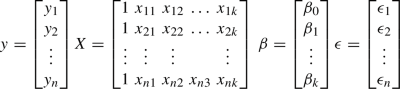
• Multiple Linear Regression (MLR) The general model of linear regression with k regressor variables after number n of observations where i=1,2,...,n is (Montgomery & Runger, 2010):

  $$\begin{aligned} y_i=\beta _0+\beta _1x_{i1}+\beta _1x_{i2}+...+\beta _kx_{ik}+\epsilon i=1,2,\ldots ,n \end{aligned}$$

  (5)

  $\epsilon$ refers to the random errors. The model can be written in the matrix form as:

  $$\begin{aligned} y=X\beta +\epsilon \end{aligned}$$

  (6)

  where:

  

  To minimise the error $\epsilon$ using the least square as stated in Montgomery and Runger (2010), the loss function L is:

  $$\begin{aligned} L=\sum _{i=1}^n \epsilon _i^2=(y-X\beta )^T (y-X\beta ) \end{aligned}$$

  To find the least square estimator ${\hat{\beta }}$:

  $$\begin{aligned} \frac{\partial {L}}{\partial {\beta }}=0 \end{aligned}$$

  and this yields:

  $$\begin{aligned} {\hat{\beta }}=(X^TX)^{-1} X^Ty \end{aligned}$$

  Next, the predicted output $\hat{y_i}$ is calculated using the equation:

  $$\begin{aligned} \hat{y_i}=\hat{\beta _0}+\sum _{j=1}^{k}\hat{\beta _j}x_{ij}\;\;\;\; i=1,2,\ldots ,n \end{aligned}$$

  (7)

  or in its equivalent matrix form:

  $$\begin{aligned} {\hat{y}}=X{\hat{\beta }} \end{aligned}$$

  (8)

  Figure 11 shows the results in terms of the predicted values compared to the actual experimental ones. In addition, some of the numerical values are shown in Table 1. After performing the MLR algorithm, around 79% of the predictions have an error that is less than 5%, whereas only less than 1% have an error over 20%.

Fig. 10

A flow chart of the test input data generation procedure

• Deep Learning (DL) A deep learning neural networks model has the exemplary illustrated in Fig. 12 which comprises: an input layer, hidden layers and an output layer. Each layer comprises a number of neurons (units) that are activated/deactivated using an activation function. Thus, by varying the number of layers, the number of neurons in each layer, or the activation function, solution quality can be improved. There are many functions that can be used as activation functions such as the step function, Sigmoid function, tanh function and Rectified Linear Unit (ReLU).

The same data used in MLR are used to train and evaluate the created deep learning model. The model was built in Python and a variety of libraries were utilised:

• Building deep learning model: Tensorflow and Keras.

• Manipulating data and splitting them into testing and training groups: Sklearn, Numpy, Pandas.

• Data visualisation Matplotlib.

The next step is to import data (in the form of a CSV file) and extract it to suit the accepted format of the model’s inputs. Then, the model is constructed of one input layer, two hidden layers (the first has 1024 neurons, and the second has 256 neurons) and the output layer. Further specifications of the model have to be configured and are shown in Table 2.

Fig. 11

Predicted energy consumption values using MLR vs. experimental values

Table 1 Exemplary results of MLR outcome

The selection of these specifications is based on multiple trials to improve the performance of the model in terms of solution quality (reduced error) and time efficiency (less calculation time). The calculation is performed using a computer whose Central Processing Unit (CPU) is Intel® Core TM i5-6500 CPU @ 3.20 GHz and with an installed Random Access Memory (RAM) of 8.00 GB. The elapsed calculation time in Python is 5.39 s.

In the implementation, data were divided into testing and training data (50% each, similar to the implementation of MLR. The results of the data fitting are shown in Fig. 13. It can be noticed that both MLR and DL could fit data properly, thus, the created models can predict drive’s energy consumption with a good level of credibility.

In relation to this, a further comparison of the outcome of both Deep Learning and MLR methods is presented in Table 3. It can be noticed that the accuracy is improved by using Deep Learning where the error $\epsilon$ decreases as shown by pie charts and the calculated values in Table 3. In general, good predictions are obtained, however, the computation cost, time and implementation effort are more when using Deep Learning.

To evaluate the results of both MLR and DL, the confidence level of 95% (significance level $\alpha =0.05$) is considered. Following the calculation of the standard error of the mean and the Z-score for a 95% confidence interval, the confidence interval is obtained (Fig. 14).

In the following, these results will be further invested in building an optimisation algorithm, then a virtual engineering model for the purpose of improving energy flexibility.

Phase II: virtual engineering and energy-flexible component

To build the digital twin of the studied component, it is necessary to (Tao et al., 2019): build a virtual representation of the physical counterpart using CAD or 3D modelling, simulate and test the physical system in a virtual environment, and establish real-time bi-directional secure connections between the physical and the cyber system. To achieve this, in addition to the elements of the experiment elements mentioned earlier in 4.2, additional tools are necessary for building the digital twin and potential tools of decision-making which are Visual Components^TM and Node-RED.

Node-RED is a programming tool originally developed by IBM based on Node.js which is an open-source JavaScript runtime environment. Node-RED provides a browser-based editor for creating flows of the programming instructions in addition to certain function blocks which accept Java codes, whereas some accept Python as well but are less developed. The flows created in Node-RED can be stored using JSON (JavaScript Object Notation), imported easily and exported for sharing with other users. Node-RED is regarded as an invaluable tool for developing IoT solutions as it enables solution developers to control and visualise the workflows of data.⁴ Another advantage of using Node-RED is the possibility of creating Graphical User Interfaces (GUIs) with dashboard elements, which enables the visualisation of parameters’ behaviour.

Visual Components, as described on the product’s homepage, is 3D manufacturing simulation software that aids machine builders, manufacturers and system integrators in developing cost-effective, simple and quick solutions. Visual Components helps to build the virtual model of the layout, work cell or the components involved in manufacturing (e.g., robots) (Mikhail et al., 2020). Moreover, it supports recording controls and the running of Python scripts to perform certain user commands. This tool’s main benefit, in relation to this work, is its ability to create the virtual model of the component, in addition to the necessary connection channels with the PLC, external server, and external software services. Furthermore, Visual Components can support the ‘reuse’ of components in future designs, making the design process more sustainable (Assad et al., 2021).

Phase II: modelling in visual components

The 3D representations of both the axis and its driving motor were provided from the manufacturer’s website (Festo). Then, they were added to a blank virtual model in the Visual Components environment as depicted in Fig. 15.

The next step is modelling both the kinematics and the controls. Visual Components defines each component with a group of behaviours and properties (Fig. 15). Control signals are stored under the behaviours in addition to the necessary codes (Python scripts) added by the user.

Component properties encompass numerical and logical values that can impact programmed behaviours, and can be mapped to the values in the physical model. For example, one of the studied axis properties is the maximum distance.

After setting the geometry, the physical behaviour of the component has to be modelled. Therefore, a translation joint is defined as $j_1$ (Fig. 15). Next, the properties of the joint such as the minimum and maximum limits, and the motion’s positive direction are entered. Once the translational joint is created, corresponding control ports are automatically generated by the software.

Fig. 12

Neural networks model

To define the “control logic”, the created translational joint has to be connected to a “Servo Controller” element. Once this controller is added, a “DriveLogic” script which contains the basic code instructions (in the form of Python functions) is created. It can be noticed that behaviour signals are linked to the component properties using the code in “DriveLogic”.

The final step in control configuration is to create signals corresponding to the ones in the PLC programme (e.g., “GetReady”, “DoHoming”), where the former enables the servo motor, and the latter instructs the motion controller to drive the joint to its zero point.

Table 2 A summary of the specifications used in deep learning model

To obtain an energy-flexible component, the ability to predict energy consumption should be added when the component is being designed as an element of the manufacturing system. Then, it has to be callable by the virtual model (which evolves into a digital twin). Furthermore, the obtained component should be adaptive, i.e., capable of reconfiguring the parameters that influence energy consumption. For the previous argument to become a reality, a collaboration between simulation capabilities, information processing means, and communication channels has to be established. Two methods of predicting energy consumption were introduced earlier, namely, MLR and Deep Learning. Taking advantage of the mathematical simplicity of MLR, and Visual Components’ behaviour scripting feature, coding MLR in a Visual Components Python script could be implemented.

Figure 16 shows that the MLR prediction method was added to the component’s behaviour, then once the simulation is run, the console output of Visual Components displays the calculated prediction of energy consumption. In this script, Eqs. 3 and 4 are executed, where the vector X is obtained from designer inputs and $\beta$ is already stored based on the findings of 4.4.2. Hence, predicted energy consumption is the scalar product of those two vectors.

Fig. 13

Predicted energy consumption values using Deep Learning vs. the actual experimental values

Deep Learning integration was not possible in Visual Components environment as it requires external Python libraries that cannot be added to the software (e.g., TensorFlow and Numpy), and also because of the complexity of the DL prediction model compared to MLR. The output of the DL model is represented by a (.h5) format, which cannot be read by Visual Components. Nevertheless, a DL method was developed using Node-RED, and will be explained later in Phase III.

Phase II: establishing connectivity to the physical model

For the developed virtual model to become a “digital twin”, successful communication with the physical model has to be established with the ability to exchange data and to report changes. A map of the communications established between the virtual model, physical model (PLC basically), KEPServerEX and Node-RED is shown in Fig. 17.

In this architecture, Node-RED serves as a platform to run and communicate with external services, e.g., Python scripts and the GUI interface. Meanwhile, KEPServerEX acts as a communication agent, ensuring the connection between the physical and cyber component’s parts to Node-RED. It should be noted that Node-RED could not be connected to Virtual Components, seemingly for security reasons. To overcome this problem, the KEPServerEX is utilised as a data exchange medium.

Using the “Connectivity” tab offered in the Visual Components environment, and using the OPC UA communication protocol, mapping of the necessary PLC code signals could be established. A major factor in simplifying this process is Siemens S7 1500 PLC OPC UA connection capability. Otherwise, KEPServerEX has to be used in addition to PLC Sim Siemens software.

Figure 18 illustrates the successful exchange of signals (real and logical) between the virtual model and PLC in two paths: “Simulation to server” and “Server to simulation”. As a result, once these signals are changed in either PLC or virtual model, the changed signal is reported to the other counterpart. In relation to energy consumption prediction, the values inputted into the virtual model and their predicted energy consumption are calculated, which can be transferred into PLC code as new industrial process parameters.

With the completion of this phase, it can be said that the digital twin of the component is born. Depending on the estimated energy consumption, the speed of the component can be changed to suit the available amount of energy or to accommodate momentary energy prices.

Table 3 A comparison between the outcomes of Deep Learning and MLR

Phase III: connecting external services to the digital twin

To increase the benefits of the developed digital twin, further external “services” will be integrated so that the system designer can query the outcome of certain design parameters. It was mentioned earlier that energy consumption prediction using DL was inapplicable in the Visual Components environment. Therefore, it will be demonstrated here how to implement DL as an external service. Furthermore, Particle Swarm Optimisation (PSO), is connected to the digital twin. An essential condition for the successful running of the external services is the communication between the digital twin and KEPServerEX, where OPC UA is utilised in a way similar to that used when connecting to the PLC. Figure 19 displays the graphical code written using Node-RED. Although the coding style is graphical, it includes some functions that are written with JavaScript and other blocks that run external Python scripts.

Fig. 14

DL and MLR data confidence intervals and the predictions

Fig. 15

Creating the virtual model of the studied component

Fig. 16

Prediction of component’s energy consumption in Visual Components environment

Fig. 17

Connectivity map of the entities involved in this work

Fig. 18

Data exchange between the digital twin and KEPServerEX

Fig. 19

External services on Node-RED

The algorithm of the graphical code is as follows:

• 1. Once there are new parameters of operation, they are passed from the digital twin to KEPServerEX.

• 2. New parameters are read from KEPServerEX then collected to form the prediction input vector.

• 3. Python DL prediction script is run with the provided input.

• 4. Prediction output is collected and sent to KEPServerEX.

• 5. Prediction output is received on the digital twin.

Similar to the way prediction using DL was integrated, PSO was programmed in a Python script and integrated (Fig. 19). The objective function can be evaluated using the energy value predicted using MLR or DL with the latter being more complex. PSO was chosen due to the following reasons (Assad et al., 2018):

• The ability to be used in multi-dimension, discontinuous and non-linear problems.

• Low computational cost.

• Its underlying concepts are simple and easy to code

• The number of parameters to adjust is fewer compared to other methods.

• It remembers the good solutions resulting from previous iterations.

• The fast convergence of the objective function.

• The final solution is not highly affected by the initial population.

The mathematical problem can be formulated as follows:

$$\begin{aligned} Minimise \ E=&f(S_f,A_{max},V_{max},CT) \nonumber \\ subjected \ to: CT&< CT_{lim} \nonumber \\ A_{max}&<A_{lim}\nonumber \\ V_{max}&<V_{lim}\nonumber \\ where\ CT>0,\&A_{max}>0, V_{max}>0 \end{aligned}$$

(9)

$CT_{lim}$ is the maximum allowed motion time, and $A_{lim},V_{lim}$ are motion constraints. E is the value of available energy so that the outcome of PSO can suit energy flexibility requirements. PSO as a service can be run by the system integrator/designer while integrating the component in a system, or by the digital twin in case of the full automation of decision-making. As Node-RED is successfully connected to the PLC, the corresponding parameters can be easily updated, leading to a new behaviour of energy consumption.

By the end of this phase, the component designed in Visual Components is exported as an independent entity with the ability to communicate with external services, and perform energy consumption prediction. Thus, component “reusability” is achieved with an Asset Administration Shell (AAS) giving the possibility for future “Plug-and-Produce”.

Bridging the gap and the response to research questions

RQ1 calls for the proactive inclusion of energy flexibility in the design of the manufacturing system. Typically, systems designers will work on modelling the components of the mechanical, electrical and control systems prior to the Testing and Commissioning phase as shown in Fig. 1. The literature on energy flexibility focuses on achieving energy flexibility for existing systems. In our approach, “proactiveness” is interpreted in the attempt to achieve this while building the components of the system. In ‘Phase I’, the component’s (electric drive) behaviour is analysed before this component is used in constructing a manufacturing station/cell. The potential of energy flexibility cannot be triggered unless the energy consumption behaviour is linked to the process’s control parameters, which is also accomplished in ‘Phase II’ by linking PLC function blocks with variables programmed in the virtual model. In the later phases of the system’s life cycle, data transfer channels established in Phases II and III continue to enable energy consumption control making the system energy flexible.

RQ2 aims at acquiring a design approach for building energy-flexible manufacturing systems. The foundation of the proposed approach is rooted in RAMI 4.0 as shown in 3.3. In Phases II and III, the engagement with the digital aspect is achieved. Thus, the aspects explained in 3, i.e., the component, the digital representation, the life cycle and the energy flexibility embedding method are realised. The asset exported by the end of Phase III is a digital presentation equipped with an IoT communication capability and contributes to achieving energy flexibility by having the energy consumption model (generated in Phase I) embedded in and the capability to access control parameters in the PLC programme, and from there to the component.

Discussion

Hands-on deliverables

Manufacturing system designers have to address the requirements of sustainability and sustainable manufacturing right from the early design phase of the life cycle. Furthermore, the designed system should leverage smart manufacturing capabilities and comply with modern design paradigms. To rise to this challenge, and with a focus on energy flexibility in manufacturing automation systems, two research questions and a sequence of the envisioned solution were suggested as a methodological approach.

From a manufacturing systems characterisation perspective, reconfigurability and flexibility were intensively discussed in the literature. Currently, Industry 4.0 inherited the characteristics of RMS. However, energy flexibility did not receive sufficient attention. The presented work contributes to the growing field of sustainable manufacturing generally, and energy flexibility particularly, by proactively employing Industry 4.0 technologies to make more flexible components, and thus more flexible manufacturing processes.

It has been shown empirically that it is feasible to mathematically describe the component’s energy consumption behaviour, and then predict it. The components developed using the suggested approach can interact with the control system (PLC in particular), whilst being digital models and when becoming digital twins. In addition, as data exchange is successfully accomplished, some signals in the PLC code can be modified flexibly. Another significant interaction is with external services. The framework developed in this work can handle further functions once coded as scripts and their inputs are provided and correctly formatted.

In the bigger picture, when components are connected to form a manufacturing cell or an assembly station, the total energy consumption can be predicted by aggregating the individual predicted energy consumptions for each of them. Therefore, energy management is achieved by quantifying the energy demand. Another dimension of energy management is to assess the component’s performance based on predefined key performance indicators (KPIs). Then, discrete event simulation can be run to evaluate a certain set of parameters against the proposed KPIs.

For energy flexibility, the proposed approach embeds energy flexibility in components starting from the design phase, unlike the approaches in the literature, which were case-specific. Moreover, the developed components represent cyber-physical components equipped with data processing and communication capabilities. Such mini-scale units can aid strategic planning and decision-making when the larger-scale system is built, thus supporting the model-based design by utilising the component-based design. Nevertheless, the realisation of such a larger-scale system will require further investment in IoT, big data and cloud applications.

Referring to the AAS Industry 4.0, and comparing it to the representation shown in Fig. 2, it can be noted that the component created using the proposed approach contains the basic elements of AAS, and align with the vision of the Industry 4.0 component.

On the design tools development side, for virtual engineering specifically, it is shown that the virtual engineering tool Visual Components could partially support energy consumption prediction. However, with the advancements in information technology, VE tools should be equipped with further computational capabilities. The solution proposed in this work relied on linking external services in order to obtain more accurate predictions. However, relying on one consistent tool to fulfil most of the design requirements can greatly aid system designers and integrators.

Although there are energy monitoring tools in the market, the solution proposed in this paper does not utilise any hardware/software from external commercial vendors; thus, there is no extra cost associated with its implementation.

Considering the transferability and scalability of the proposed approach, the tools used to build an energy-flexible component are representative of their main technologies, and not the only possible choices. For example, Node-RED and KepServerEX are possible tools for utilising the OPC UA communication protocol. Similarly, DL and MLR are commonly used and open-source Python libraries for machine learning which have alternatives in Matlab and Java, etc. With the flexibility provided by Node-RED, modules/codes from other software tools can be connected to the virtual models allowing the designer/decision-maker to take advantage of their available tools.

A focal point for the successful implementation of the proposed approach is the modelling of energy consumption. Performing this is not strictly limited to machine learning as it has been conducted in this work. Analytical and physical models can replace the ML model as long as their outcome is transferable to the virtual model. For example, the output of an analytical model written in Matlab can be sent to the IoT platform using Matlab’s OPC UA library. However, Matlab does not provide any free toolboxes. It should be noted that the content of the machine learning box on Node-Red can be filled with another ML algorithm such as Random Forest or k-Nearest Neighbours.

The electric drive is an example of the “component” within the wider broader context which can be a hydraulic or a pneumatic component. Afterwards, once its energy consumption is modelled, energy flexibility is managed by the algorithms that coordinate data transfer between the virtual model and its counterpart, and can change control parameters on the PLC.

Based on the aforementioned arguments, and to answer the research questions put forward earlier, embedding the energy consumption behaviour of manufacturing systems’ components starting from the design phase is the pillar of a proactive energy flexibility design. The technical implementation of this vision is through creating the corresponding energy consumption models at the design phase. The contribution of Industry 4.0, specifically IoT, is enabling the quick acquisition of the component’s related data (the physical aspect), and the ability to transfer it to the cyber counterpart and the cyber entities/services connected to it (RQ1). Considering that the modern manufacturing systems will comply with Industry 4.0, the design approach of energy-flexible components has to be harmonised with I4.0 components, so that they can be successfully integrated and utilised to construct an energy-flexible system (RQ2).

Limitations

During the course of this research, several challenges were encountered that should be acknowledged and considered:

• The sampling rate of power analyser and KEPServerEX: for measuring power, and eventually energy, a power analyser was used. However, it was not possible to obtain acceptable data quality with a sampling rate of less than 100 ms.

• The fixed load for the component: when collecting data to quantify the energy consumption of the studied component (electric drive, motor and axis), the load on the component was fixed. For future studies, the load can be varied and added as a variable in the energy consumption prediction method.

• The complexity of the communications in the proposed approach: a map of the communication network utilised in this work was presented earlier (Fig. 17). However, it is not always easy to connect a variety of servers, clients, services and simulators. Therefore, this communication network has to be simplified in the future in order to reduce the resultant complexity.

• Resource and skills requirements: in order to successfully create an energy-flexible component, a procedure has been developed and a variety of tools were invested (e.g. virtual engineering, database management and PLC programming). Additionally, various programming and communication skills were required. Consequently, in industrial practice, users may not possess all the skills needed to follow the procedure in full.

Conclusion and future work

As the concerns about climate change grow, and energy prices rise, the urge to develop sustainable manufacturing becomes prevalent. Solutions developed to contribute to sustainable manufacturing enhancement have to take full advantage of the available technologies. Delivering sustainability has always been closely tied to the anatomy of the manufacturing system. Therefore, there is a strong link between the architecture of the manufacturing system and its underlying sustainability potential. Although research on energy management continues to embrace Industry 4.0 technologies, using those technologies towards energy flexibility is still limited. Based on these facts, the current work targets achieving energy flexibility from a cyber-physical systems perspective and in line with the Industry 4.0 paradigm.

The approach presented in this work addresses this issue starting from the design phase with the vision of covering the life cycle of the manufacturing system. It aims to provide a comprehensive understanding of how lower-level components respond to energy demands. Thus, a component-based design consistent with Industry 4.0 component design is suggested. A procedure is developed in order to model the energy consumption behaviour of the component, then to create the virtual model that evolves into a digital twin once data communication channels are successfully established. When doing so, full advantage of data is taken thanks to IoT technology.

In the conducted three-phase implementation, an electric drive serves as an exemplar of a manufacturing component, where its energy consumption is modelled using machine learning techniques, namely Multiple Linear Regression and Deep Learning (Phase I). In Phase II, the virtual model of the drive is created, and the energy consumption behaviour is integrated into it. Then, the digital twin is built using suitable IoT and virtual engineering tools. In Phase III, external services (e.g., Particle Swarm Optimisation, and Deep Learning) are connected to the digital twin in order to support both the design and real-time operation. Furthermore, the developed components are designed to be reusable contributing to design sustainability, and configurable in order to respond to changes in energy provision/prices, thus enhancing energy flexibility.

With the widespread use of IoT and its integration into various domestic and industrial applications, its sensors, communication devices and software tools are becoming less expensive than before. Simultaneously, the digitalisation of manufacturing systems is on the rise, and including sustainability in design is gaining significant importance. Accordingly, using the proposed approach in an industrial environment is now practically applicable. Although the implementation takes place on an electrical drive, other types of components can be similarly modelled.

For manufacturing systems designed using the proposed approach, it is beneficial to extend the current work by examining the interaction with higher control levels such as Energy Resources Planning (ERP) and Production Planning and Control (PPC) for improved energy flexibility. Thus, predictive models for higher levels can be created. Also, in relation to the above-mentioned interaction with the energy provision system, further planning scenarios can be explored.

In another future research direction, the increased engagement of IoT devices and data storage introduces greater complexity to the manufacturing system. Therefore, it is necessary to investigate the impact of adding energy-related modules and explore methods to mitigate the resulting complexity.

References

Alkan, B., & Harrison, R. (2019). A virtual engineering based approach to verify structural complexity of component-based automation systems in early design phase. Journal of Manufacturing Systems, 53, 18–31. https://doi.org/10.1016/j.jmsy.2019.09.001
Angizeh, F., Montero, H., Vedpathak, A., & Parvania, M. (2020). Optimal production scheduling for smart manufacturers with application to food production planning. Computers & Electrical Engineering, 84, 106609. https://doi.org/10.1016/j.compeleceng.2020.106609
Angizeh, F., & Parvania, M. (2019). Stochastic risk-based flexibility scheduling for large customers with onsite solar generation. IET Renewable Power Generation, 13(14), 2705–2714. https://doi.org/10.1049/iet-rpg.2019.0233
Assad, F., Rushforth, E., Ahmad, B., Harrison, R., et al. (2018). An approach of optimising s-curve trajectory for a better energy consumption. In: 2018 IEEE 14th International Conference on Automation Science and Engineering (CASE), pp. 98–103. https://doi.org/10.1109/COASE.2018.8560587. IEEE
Assad, F., Konstantinov, S., Rushforth, E. J., Vera, D. A., & Harrison, R. (2021). Virtual engineering in the support of sustainable assembly systems. Procedia CIRP, 97, 367–372. https://doi.org/10.1016/j.procir.2020.05.252
Bauer, D., Abele, E., Ahrens, R., Bauernhansl, T., Fridgen, G., Jarke, M., Keller, F., Keller, R., Pullmann, J., Reiners, R., et al. (2017). Flexible it-platform to synchronize energy demands with volatile markets. Procedia CIRP, 63, 318–323. https://doi.org/10.1016/j.procir.2017.03.088
Beier, J., Thiede, S., & Herrmann, C. (2017). Energy flexibility of manufacturing systems for variable renewable energy supply integration: Real-time control method and simulation. Journal of Cleaner Production, 141, 648–661. https://doi.org/10.1016/j.jclepro.2016.09.040
Boss, B., Malakuti, S., Lin, S., Usländer, T., Clauer, E., Hoffmeister, M. & Stojanovic, L. (2020). Digital twin and asset administration shell concepts and application in the industrial internet and industrie 4.0. https://www.plattform-i40.de/IP/Redaktion/EN/Downloads/Publikation/Digital-Twin-and-Asset-Administration-Shell-Concepts.pdf?__blob=publicationFile &v=9. Accessed: 03/02/2022
Brugger, M., Götz, G., Richter, C., & Reinhart, G. (2017). Study on energy efficiency and flexibility in machinery and production. Applied Mechanics and Materials, 871, 103–114. https://doi.org/10.4028/www.scientific.net/AMM.871.103
Carabin, G., & Scalera, L. (2020). On the trajectory planning for energy efficiency in industrial robotic systems. Robotics, 9(4), 1–13. https://doi.org/10.3390/robotics9040089
Chen, X., Li, C., Tang, Y., & Xiao, Q. (2018). An internet of things based energy efficiency monitoring and management system for machining workshop. Journal of Cleaner Production, 199, 957–968. https://doi.org/10.1016/j.jclepro.2018.07.211
Diaz, J. L. C., & Ocampo-Martinez, C. (2019). Energy efficiency in discrete-manufacturing systems: Insights, trends, and control strategies. Journal of Manufacturing Systems, 52, 131–145. https://doi.org/10.1016/j.jmsy.2019.05.002
Feng, Y., Wang, Q., Gao, Y., Cheng, J., & Tan, J. (2018). Energy-efficient job-shop dynamic scheduling system based on the cyber-physical energy-monitoring system. IEEE Access, 6, 52238–52247. https://doi.org/10.1109/ACCESS.2018.2869048
Foumani, M., & Smith-Miles, K. (2019). The impact of various carbon reduction policies on green flowshop scheduling. Applied Energy, 249, 300–315. https://doi.org/10.1016/j.apenergy.2019.04.155
Graßl, M., Vikdahl, E. & Reinhart, G. (2014). A petri-net based approach for evaluating energy flexibility of production machines. In: Enabling Manufacturing Competitiveness and Economic Sustainability, pp. 303–308. Springer. https://doi.org/10.1007/978-3-319-02054-9_51
Harrison, R., Vera, D., & Ahmad, B. (2016). Engineering methods and tools for cyber-physical automation systems. Proceedings of the IEEE, 104(5), 973–985. https://doi.org/10.1109/JPROC.2015.2510665
Hojnik, J., Ruzzier, M., & Ruzzier, M. K. (2019). Transition towards sustainability: Adoption of eco-products among consumers. Sustainability (Switzerland). https://doi.org/10.3390/su11164308
Ivanov, D., Sokolov, B., Chen, W., Dolgui, A., Werner, F., & Potryasaev, S. (2021). A control approach to scheduling flexibly configurable jobs with dynamic structural-logical constraints. IISE Transactions, 53(1), 21–38. https://doi.org/10.1080/24725854.2020.1739787
Javied, T., Rackow, T., Stankalla, R., Sterk, C., & Franke, J. (2016). A study on electric energy consumption of manufacturing companies in the german industry with the focus on electric drives. Procedia CIRP, 41, 318–322. https://doi.org/10.1016/j.procir.2015.10.006
Jiang, W., & Chen, X. (2016). Optimal strategies for manufacturer with strategic customer behavior under carbon emissions-sensitive random demand. Industrial Management & Data Systems, 116(4), 759–776. https://doi.org/10.1108/IMDS-08-2015-0321
Kannan, K., & Arunachalam, N. (2019). A digital twin for grinding wheel: an information sharing platform for sustainable grinding process. Journal of Manufacturing Science and Engineering, 10(1115/1), 4042076.
Katchasuwanmanee, K., Bateman, R., & Cheng, K. (2016). Development of the energy-smart production management system (e-proman): A big data driven approach, analysis and optimisation. Proceedings of the Institution of Mechanical Engineers, Part B: Journal of Engineering Manufacture, 230(5), 972–978. https://doi.org/10.1177/0954405415586711
Köberlein, J., Bank, L., Roth, S., Köse, E., Kuhlmann, T., Prell, B., Stange, M., Münnich, M., Flum, D., Moog, D., et al. (2022). Simulation modeling for energy-flexible manufacturing: Pitfalls and how to avoid them. Energies, 15(10), 3593. https://doi.org/10.3390/en15103593
Konstantinov, S., Assad, F., Ahmad, B., Vera, D. A., & Harrison, R. (2022). Virtual engineering and commissioning to support the lifecycle of a manufacturing assembly system. Machines, 10(10), 939. https://doi.org/10.3390/machines10100939
Lee, S.-M., Harrison, R. & West, A.A. (2004). A component-based distributed control system for assembly automation. In: 2nd IEEE International Conference on Industrial Informatics, 2004. INDIN’04. 2004, pp. 33–38. https://doi.org/10.1109/INDIN.2004.1417298 . IEEE
Li, Y., Wang, Z., Yang, H., Zhang, H., & Wei, Y. (2023). Energy-optimal planning of robot trajectory based on dynamics. Arabian Journal for Science and Engineering, 48(3), 3523–3536. https://doi.org/10.1007/s13369-022-07185-7
Materi, S., D’Angola, A., & Renna, P. (2020). A dynamic decision model for energy-efficient scheduling of manufacturing system with renewable energy supply. Journal of Cleaner Production, 270, 122028. https://doi.org/10.1016/j.jclepro.2020.122028
Mattmann, C.A. (2020). Machine Learning with TensorFlow. Manning. Available from https://www.manning.com/books/machine-learning-with-tensorflow-second-edition
Mawson, V. J., & Hughes, B. R. (2019). The development of modelling tools to improve energy efficiency in manufacturing processes and systems. Journal of Manufacturing Systems, 51, 95–105. https://doi.org/10.1016/j.jmsy.2019.04.008
Ma, S., Zhang, Y., Liu, Y., Yang, H., Lv, J., & Ren, S. (2020). Data-driven sustainable intelligent manufacturing based on demand response for energy-intensive industries. Journal of Cleaner Production, 274, 123155. https://doi.org/10.1016/j.jclepro.2020.123155
Medojevic, M., Villar, P. D., Cosic, I., Rikalovic, A., Sremcev, N., & Lazarevic, M. (2018). Energy management in Industry 4.0 ecosystem: A review on possibilities and concerns. Annals of DAAAM & Proceedings,29. https://doi.org/10.2507/29th.daaam.proceedings.097
Mikhail, M., Bharti, S. & Alavizadeh, A. (2020). Incorporating visual components simulation software with the programming industrial robots course. ASEE. Available from https://www.asee.org/public/conferences/172/papers/28790/view
Moghaddam, M., Cadavid, M. N., Kenley, C. R., & Deshmukh, A. V. (2018). Reference architectures for smart manufacturing: A critical review. Journal of Manufacturing Systems, 49, 215–225. https://doi.org/10.1016/j.jmsy.2018.10.006
Montgomery, D. C., & Runger, G. C. (2010). Applied Statistics and Probability for Engineers (pp. 456–457). John Wiley & Sons.
Nienke, S., Frölian, H., Zeller, V. & Schuh, G. (2017). Energy-management 4.0: roadmap towards the self-optimising production of the future. In: Proceedings of the 6th International Conference on Informatics, Environment, Energy and Applications, pp. 6–10. https://doi.org/10.1145/3070617.3070621
Pease, S. G., Trueman, R., Davies, C., Grosberg, J., Yau, K. H., Kaur, N., Conway, P., & West, A. (2018). An intelligent real-time cyber-physical toolset for energy and process prediction and optimisation in the future industrial internet of things. Future Generation Computer Systems, 79, 815–829. https://doi.org/10.1016/j.future.2017.09.026
Pei, W., Ma, X., Deng, W., Chen, X., Sun, H., & Li, D. (2018). Industrial multi-energy and production management scheme in cyber-physical environments: a case study in a battery manufacturing plant. IET Cyber-Physical Systems: Theory & Applications, 4(1), 13–21. https://doi.org/10.1049/iet-cps.2018.5029
Pelzer, A., Lombardi, P., Arendarski, B., & Komarnicki, P. (2016). An innovative energy management system for the integration of volatile energy into industrial processes. International Journal of Energy Production and Management, 1(4), 339–348. https://doi.org/10.2495/EQ-V1-N4-339-348
Plattform Industrie 4.0: RAMI4.0 – a reference framework for digitalisation. https://www.plattform-i40.de/PI40/Redaktion/EN/Downloads/Publikation/rami40-an-introduction.pdf?__blob=publicationFile &v=7. Accessed: 06/03/2021 (2018)
Popp, R.S.-H., Liebl, C., & Zaeh, M. F. (2017). Evaluation of the energy flexible operation of machine tool components. Procedia CIRP, 63, 76–81. https://doi.org/10.1016/j.procir.2017.02.037
Rocca, R., Rosa, P., Sassanelli, C., Fumagalli, L., & Terzi, S. (2020). Integrating virtual reality and digital twin in circular economy practices: a laboratory application case. Sustainability, 12(6), 2286. https://doi.org/10.3390/su12062286
Rödger, J.-M., Beier, J., Schönemann, M., Schulze, C., Thiede, S., Bey, N., Herrmann, C., & Hauschild, M. Z. (2020). Combining life cycle assessment and manufacturing system simulation: Evaluating dynamic impacts from renewable energy supply on product-specific environmental footprints. International Journal of Precision Engineering and Manufacturing-Green Technology. https://doi.org/10.1007/s40684-020-00229-z
Roth, S., Kalchschmid, V., & Reinhart, G. (2021). Development and evaluation of risk treatment paths within energy-oriented production planning and control. Production Engineering. https://doi.org/10.1007/s11740-021-01043-5
Sajadi, A., Strezoski, L., Strezoski, V., Prica, M., & Loparo, K. A. (2018). Integration of renewable energy systems and challenges for dynamics, control, and automation of electrical power systems. Wiley Interdisciplinary Reviews Energy and Environment. https://doi.org/10.1002/wene.321
Saldivar, A.A.F., Li, Y., Chen, W.-n., Zhan, Z.-h., Zhang, J. & Chen, L.Y. (2015). Industry 4.0 with cyber-physical integration: A design and manufacture perspective. In: 2015 21st International Conference on Automation and Computing (ICAC), pp. 1–6. https://doi.org/10.1109/IConAC.2015.7313954 . IEEE
Schneider, G. F., Wicaksono, H., & Ovtcharova, J. (2019). Virtual engineering of cyber-physical automation systems: The case of control logic. Advanced Engineering Informatics, 39, 127–143. https://doi.org/10.1016/j.aei.2018.11.009
Shrouf, F., & Miragliotta, G. (2015). Energy management based on Internet of Things: practices and framework for adoption in production management. Journal of Cleaner Production, 100, 235–246. https://doi.org/10.1016/j.jclepro.2015.03.055
Stock, T., & Seliger, G. (2016). Opportunities of sustainable manufacturing in industry 4.0. Procedia Cirp, 40, 536–541. https://doi.org/10.1016/j.procir.2016.01.129
Tao, F., Cheng, J., Qi, Q., Zhang, M., Zhang, H., & Sui, F. (2018). Digital twin-driven product design, manufacturing and service with big data. The International Journal of Advanced Manufacturing Technology, 94(9), 3563–3576. https://doi.org/10.1007/s00170-017-0233-1
Tao, F., Sui, F., Liu, A., Qi, Q., Zhang, M., Song, B., Guo, Z., Lu, S.C.-Y., & Nee, A. (2019). Digital twin-driven product design framework. International Journal of Production Research, 57(12), 3935–3953. https://doi.org/10.1080/00207543.2018.1443229
Tao, F., Zuo, Y., Da Xu, L., Lv, L., & Zhang, L. (2014). Internet of things and bom-based life cycle assessment of energy-saving and emission-reduction of products. IEEE Transactions on Industrial Informatics, 10(2), 1252–1261. https://doi.org/10.1109/TII.2014.2306771
UN: Sustainable Development Goals, 7 Affordable and clean energy. https://www.un.org/sustainabledevelopment/energy/. Accessed: 21/11/2018 (2015)
UN: Sustainable Development Goals, 9 Industry, innovation, and infrastructure. https://www.un.org/sustainabledevelopment/infrastructure-industrialization/. Accessed: 21/11/2018 (2015)
Wagner, C., Grothoff, J., Epple, U., Drath, R., Malakuti, S., Grüner, S., Hoffmeister, M. & Zimermann, P. (2017). The role of the Industry 4.0 asset administration shell and the digital twin during the life cycle of a plant. In: 2017 22nd IEEE International Conference on Emerging Technologies and Factory Automation (ETFA), pp. 1–8. https://doi.org/10.1109/ETFA.2017.8247583 . IEEE
Wang, Y., Zhang, M. & Zuo, Y. (2016). Potential applications of IoT-based product lifecycle energy management. In: 2016 IEEE 11th Conference on Industrial Electronics and Applications (ICIEA), pp. 1999–2002. https://doi.org/10.1109/ICIEA.2016.7603917 . IEEE
Wang, J., Huang, Y., Chang, Q., & Li, S. (2019). Event-driven online machine state decision for energy-efficient manufacturing system based on digital twin using max-plus algebra. Sustainability, 11(18), 5036. https://doi.org/10.3390/su11185036
Wang, P., & Luo, M. (2021). A digital twin-based big data virtual and real fusion learning reference framework supported by industrial internet towards smart manufacturing. Journal of Manufacturing Systems, 58, 16–32. https://doi.org/10.1016/j.jmsy.2020.11.012
Wang, W., Yang, H., Zhang, Y., & Xu, J. (2018). IoT-enabled real-time energy efficiency optimisation method for energy-intensive manufacturing enterprises. International Journal of Computer Integrated Manufacturing, 31(4–5), 362–379. https://doi.org/10.1080/0951192X.2017.1337929
Yu, C.-M., Chien, C.-F., & Kuo, C.-J. (2017). Exploit the value of production data to discover opportunities for saving power consumption of production tools. IEEE Transactions on Semiconductor Manufacturing, 30(4), 345–350. https://doi.org/10.1109/TSM.2017.2750712
Zhang, C., Wang, Z., Ding, K., Chan, F. T., & Ji, W. (2020). An energy-aware cyber physical system for energy big data analysis and recessive production anomalies detection in discrete manufacturing workshops. International Journal of Production Research, 58(23), 7059–7077. https://doi.org/10.1080/00207543.2020.1748904
Zhang, M., & Yan, J. (2021). A data-driven method for optimizing the energy consumption of industrial robots. Journal of Cleaner Production, 285, 124862.
Zhang, H., Yan, Q., & Wen, Z. (2020). Information modeling for cyber-physical production system based on digital twin and automationml. The International Journal of Advanced Manufacturing Technology. https://doi.org/10.1007/s00170-020-05056-9
Zhu, J., Lu, Y., Song, Z., Shao, X., & Yue, X.-G. (2023). The choice of green manufacturing modes under carbon tax and carbon quota. Journal of Cleaner Production, 384, 135336. https://doi.org/10.1016/j.jclepro.2022.135336
ZWEI: Status Report: The Reference Architectural Modal Industrie 4.0 (RAMI 4.0). https://www.zvei.org/fileadmin/user_upload/Themen/Industrie_4.0/Das_Referenzarchitekturmodell_RAMI_4.0_und_die_Industrie_4.0-Komponente/pdf/5305_Publikation_GMA_Status_Report_ZVEI_Reference_Architecture_Model.pdf. Accessed: 09/06/2021 (2015)
Acknowledgements
The authors acknowledge the support of the Doctoral College at the University of Warwick, United Kingdom for funding this work. The authors sincerely thank Dr. Tony Salloom for his valuable help.
Author information
Authors and Affiliations
Corresponding author
Ethics declarations
Competing interest
The authors declare that they have no known competing financial interests or personal relationships that could have appeared to influence the work reported in this paper.
Additional information
Publisher's Note
Springer Nature remains neutral with regard to jurisdictional claims in published maps and institutional affiliations.
Rights and permissions
Open Access This article is licensed under a Creative Commons Attribution 4.0 International License, which permits use, sharing, adaptation, distribution and reproduction in any medium or format, as long as you give appropriate credit to the original author(s) and the source, provide a link to the Creative Commons licence, and indicate if changes were made. The images or other third party material in this article are included in the article’s Creative Commons licence, unless indicated otherwise in a credit line to the material. If material is not included in the article’s Creative Commons licence and your intended use is not permitted by statutory regulation or exceeds the permitted use, you will need to obtain permission directly from the copyright holder. To view a copy of this licence, visit http://creativecommons.org/licenses/by/4.0/.
About this article
Cite this article
Assad, F., Rushforth, E.J. & Harrison, R. A component-based design approach for energy flexibility in cyber-physical manufacturing systems. J Intell Manuf (2023). https://doi.org/10.1007/s10845-023-02280-4
Received:
Accepted:
Published:
DOI: https://doi.org/10.1007/s10845-023-02280-4