OVI-3: A NoSQL visual query system supporting efficient anti-joins

Abstract

The aim of this work was to develop a technique to speed up complex joins in an incremental visual query system. When designing a visual, highly interactive interface for ad-hoc (read-only) queries, fast response times are of paramount importance. While a column-oriented DBMS reduces the inherent latency found in relational DBMS, there is still the question of how to index the data, especially so as to support complex joins. Equi-joins that involve a many-to-many relationship are an example of complex joins that arise frequently and whose efficient processing is essential for fast query processing. We present OVI-3, a NoSQL visual query system based on incremental querying that uses a simple directory-based indexing scheme for faster processing of such complex joins. The system has been piloted using real data from a student database at Aalto University. The results demonstrated that for certain complex joins the presented indexing scheme outperforms SQL queries from a data server, especially for queries involving anti-joins (negation), where OVI-3 provided an orders of magnitude speed improvement.

1 Introduction

Besides being intuitive and easy to use, a VQS must also provide fast response times. This is especially true when using incremental query formulation, a paradigm made popular back in the 1990’s (Ahlberg & Shneiderman, 1994; Tanin et al., 1996). Incremental querying is based on interactively browsing the contents of a database (Larson, 1986) through filters. Interactive browsing is a user-friendly approach whereby the user simply modifies any of the existing query constraints by further restricting or relaxing them, thereby immediately producing a new answer set. In Tanin et al. (1996), the authors proposed that the term ‘immediately’ should refer to a delay of no more than one second, the time period that a user can afford to wait at each step for the new data (corresponding to the modified constraints) to appear. Later studies (Liu and Heer, 2014; Eichmann et al., 2020) have halved this threshold latency to 0.5s.

Incremental querying assumes a continuous display (Ahlberg & Shneiderman, 1994), whereby the user starts with a subset of the data considered to be relevant by the developer and then, incrementally, zooms in/out by placing further restrictions or relaxing some of the existing ones. Users thus explore, through visual elements, a subset of the database, the active subset (Derthick et al., 1999), and keep refining the query step-by-step until the active subset holds all the data the user is looking for and nothing else. When that is the case, the active subset becomes the final result set and the query can be considered to have successfully completed.

A key factor that can dramatically enhance response times for read-only queries is the data layout or the data arrangement architecture. This architecture can either be the traditional row-based arrangement found in relational databases or it can be column-based, as typically used in NoSQL approaches (Gessert et al., 2017). A column-based architecture stores each column separately on disk to speed up queries that only retrieve a few attributes from each relation. Even if the data layout is column-based, the result set must still be returned to the user in a row-based format, at which point the columns need to be assembled into a set of rows, known as tuple reconstruction (Abadi et al., 2008; Idreos et al., 2009).

Joins occur frequently in queries and remain a costly operation both in row-based (Mishra & Eich, 1992; Li & Ross, 1999) and column-based architectures (Idreos et al., 2009). Joins are a known bottleneck for query times, especially when the query involves a many-to-many, or M:N relationship. An M:N relationship arises when the relationship between two entities R and S is such that a tuple or row from one relation R can be joined to several tuples from another relation S and vice versa (Blasgen & Eswaran, 1977). Semantically, for instance, the relationship between students and courses at a university is M:N because a student can take several courses, and any given course in turn is taken by several students. For brevity, when there is an M:N relationship between two entities R and S, we refer to the join (assumed to be an equi-join) between the involved relations as an M:N join.

This article is about developing a VQS based on incremental querying that provides efficient support for complex joins that arise in M:N relationships. We use a technique of directory-based indexing or briefly DBI, presented in detail in Section 3.7. Based on this DBI approach, we have developed a prototype VQS that supports incremental querying, named OVI-3 (for “Offline Visual Incremental querying”). OVI-3 has been used in a pilot project to monitor students’ academic progress at Aalto University.

OVI-3 is the culmination of some new ideas to improve on a previous VQS, OVI-2, short for Oodi’s Visual Interface (El-Mahgary & Soisalon-Soininen, 2015) that was successfully used for several years by academic counsellors to perform ad-hoc queries on Aalto University’s student database, known as Oodi. The ‘2’ in the name OVI-2 is not a version number (there never was an OVI-1) but rather denotes the fact that OVI-2 used a two-stage querying. The first stage would return the user a superset of the required data, the result set of which was re-arranged into a more user-friendly temporary database created from scratch. The second stage then allowed the user to perform fast in-depth querying on the just created smaller dataset that was stored locally.

As to the ‘3’ in the name OVI-3, it signifies the additional step required to regularly transfer data from the university database server to OVI-3 and build a new dataset using the DBI technique. The data transfer is handled through a separate batch application as described in Section 3.7.2. OVI-3 users thus never connect to the university database server. As we shall see in Section 4.6, the DBI approach can dramatically improve the performance of M:N joins, and is especially useful in queries that involve anti-joins, commonly known as negations. The present article is not a comprehensive treatment on the OVI-3 system, but rather focuses on techniques that support the implementation of fast joins and anti-joins in M:N relationships.

Regarding the arrangement of this article, Section 2 presents a minimal student database together with a review of Datalog and a look at the concept of negation. Datalog is a convenient tool for discussing joins and negations in queries, especially since the queries in our VQS are not handled through SQL. Section 3 briefly discusses some of the main concepts behind modern VQS together with their fundamental characteristics. Implementation issues are briefly dealt with in Section 3.7. Section 4 presents the visual querying aspects of OVI-3 through an example query and then contrasts the query results when using OVI-3 with an equivalent query that is run on the actual university’s relational database server. Finally, conclusions are drawn in Section 5.

2 Concepts and terminology related to M:N joins

This section presents some important terminology and concepts related to M:N joins.

2.1 A simple toy database schema

Consider a basic toy database for managing courses taken by university students. For now we focus on just two tables, namely Students (Table 1), Courses (not shown) and CoursesTaken (Table 2). There is an M:N (many-to-many) relationship between tables Students and Courses, because a student can take several courses, and any given course can be taken by several students. In this case the table CoursesTaken, which contains column StudentID as a foreign key, is known as the join table or the bridge table (Ahmed et al., 2013).

Table 1 Three students in the toy table Students along with their four attributes. Note the lack of any capitals in the table entries, which are reserved for Datalog variables

Table 2 Table CoursesTaken contains five course instances taken by the students

The OVI-3 approach essentially re-organizes the data into a column-based format where the keys that take part in an M:N join are stored separately using the DBI technique. As this article is about the efficient implementation of such joins (i.e., M:N joins and M:N anti-joins), we refer to the join between tables Students and CoursesTaken as a primal join.

A primal join thus always derives from an M:N relationship. Analogously, we refer to the anti-join between tables Students and CoursesTaken as a primal anti-join. Both of these join concepts are defined with the help of an example in Section 2.3.

2.2 The concept of viewpoints and the value store

We postulate that one of the tables in a primal join is crucial with respect to the query, as it identifies the semantic entity or (principal) concept (Soylu et al., 2016) in which the user is interested. This principal concept is similar to what Benzi et al. (1996) refer to as a viewpoint, to which we will return shortly. We call the table in the primal join that represents the principal concept the primal tableT_prim,¹ while the other table is called the M:N foreign key table, denoted T_frgn.

Now consider a query that finds students who took course ‘MECH-1001’ and that displays, for such students, the courses they took. In such a case the query’s principal concept, or viewpoint, is students, T_prim refers to the table Students and T_frgn refers to the table CoursesTaken. Information on courses will be treated as nested results (Bakke and Karger, 2016), that is, the courses taken by a student are considered an extended property of each individual student in the result set.

Our notion of a viewpoint is similar to the ‘anchor table’ in Stonebraker et al. (2005), and in our case determines the choice of T_prim. The use of viewpoints is what brings intelligence to OVI-3, for given a viewpoint, T_prim is immediately known, and from this T_frgn is deduced. This lays the foundation for efficiently performing certain types of joins and anti-joins, as will be shown in Section 2.4. For a given VQS, the programmer only needs to create a limited number of viewpoints depending on the users’ needs. A user normally selects a viewpoint just after starting the VQS, thereby determining the set of restrictions available and thus also changing the look of the VQS. With OVI-3, only two viewpoints are needed in our toy example: (i) a ‘Students’ viewpoint to retrieve students along with the courses they have taken and (ii) an ‘Instructors’ viewpoint for retrieving instructors along with the courses they have taught.

Because OVI-3 is geared towards a column-based data layout, a relation or table is actually implemented as a value store and hence we consider the three terms relation, table, and value store as synonyms. Since in our case a value store contains several attributes for each key, it is not a key-value store, nor is it exactly a wide-column store as there is only one level of indexing (keys) (Gessert et al., 2017). A value store can be considered a table, since it is equipped with a primary key and may contain foreign keys that are part of its compound primary key. However, unlike a table, a value store is normally accessed only via its primary key and not via joins. Moreover, normalization rules for normal forms 2NF and above are relaxed for a value store.

2.3 A review of Datalog and its relation to present work

This section provides a brief review of the Datalog query language, which is attractive for our purposes due to its lack of keywords and its close ties to relational databases. We also discuss the relationship of Datalog to some key concepts of this article.

Like SQL, Datalog is a declarative language. Unlike SQL, however, Datalog is based on logic programming and a program contains a set of one or more predicates. A predicate is made up of its name, followed by a fixed number of arguments (variables or constants) listed within parentheses, and evaluates to a Boolean value (Molina et al., 2009). The combination of a predicate followed by its arguments is known as an atom (Greco and Molinaro, 2016) and is the equivalent of a functional call in traditional programming languages (Molina et al., 2009).

Predicates are in Datalog the building blocks of rules. The common syntax for a rule is the head part, followed by the symbol ‘:-’ (which can be read as ‘if’) and a body part that follows. A rule may consist of a single atom, with an empty body part (and no preceding ‘:-’ symbol). In case its arguments are all constants, the rule is reduced to a grounded fact, known simply as a fact (Ceri et al., 1989; Greco & Molinaro, 2016). Using the notation from Sippu and Soisalon-Soininen (1996) and assuming arguments are represented as vectors ($\bar {X}$), an example of a rule R with predicate p at its head and a body made up of predicates p₁...p_n would be

$$R : p(\bar{X}) \text{:-} p_{1}(\bar{X_{1}}),\dots,p_{n}(\bar{X_{n}}).$$

(1)

All predicates in the body of a rule R must evaluate to true for the rule’s head predicate p itself to evaluate to true, which is why the body is known as a conjunction (Greco & Molinaro, 2016). A rule where the head predicate p evaluates to true in case just any single predicate among $p_{1},\dots ,p_{n}$ in the body evaluates to true would be a disjunction. Datalog however does not have direct support for disjunctions, so representing a disjunction of n body atoms requires n rules, where each rule R_i, $i = 1,\dots ,n$, consists of the head atom $p(\bar {X})$ and a single atom $p_{i}(\bar {X_{i}})$ in its body.

Each row or tuple i in a relational table T can be viewed as a fact $F_{T_{i}}$ in Datalog. For instance, referring to the toy relation Students in Table 1, we could represent its first row as the fact students(22,taneli,huiskanen,mech_eng). Because facts actually exist in the database, a predicate associated directly with facts is considered an extensional database predicate (Ceri et al., 1989), and such a predicate together with its arguments is known as an extensional atom (Greco & Molinaro, 2016).

As we are not interested in recursive queries, we omit the possibility of recursion in Datalog, and consider a Datalog program as a collection of rules that are grounded in a dataset comprised of facts. A simple example of a Datalog program is presented in Listing 1 below, where the dataset (not shown) is assumed to be derived directly from Tables 1 and 2.

Listing 1

A Datalog program consisting of a single rule or query to retrieve the student IDs of students who have taken a given course as specified by the user-assigned variable CourseID

We continue with the relation Students and the predicate students, but instead of constants, we now use variables for all the arguments in the predicate. We thus obtain the atom students(StudentID, FirstName, LastName, Major), which represents the whole Students relation, encompassing the full dataset comprising three rows and their four attributes. Because this formula physically corresponds to a relation in the database schema, it also is an example of an extensional atom.

Extensional predicates cannot by their nature appear in the head of rules, and predicates serving in that role are called intensional predicates, or if their arguments are included, derived atoms (Greco & Molinaro, 2016). A derived atom does not have a direct correlate in the relational database and it is precisely derived atoms such as $p(\bar {X})$ in rule R in (1) that allow inference, or query rules consisting of a head and a body to be constructed.

Before looking closer into the design of rules, a few notes on variables. In Datalog, variable names start with a capital first letter, while predicate names and constants are written fully in lowercase. In some cases the value for a variable is provided as a parameter by the user at the start of a program and remains unchanged throughout the program’s execution. To distinguish between such user-assigned (parameter) variables and other (free) variables, we use the caret (ˆ) suffix notation to indicate the former condition. A user-assigned variable with name VarName will thus be written as VarNameˆ.

In the execution of a Datalog program, new facts are derived from known ones through the application of rules and the instantiation of variables. In instantiation, the variables in a predicate are substituted by the values of corresponding constants from a matching fact i.e., a fact whose name and arity match those of the predicate. (For details, see Greco and Molinaro (2016).)

Consider Listing 1 where the program consists of a single rule. At the head of the rule is the derived atom studentstookcourse with its two arguments, free variable StudentID and user-assigned variable CourseID. The value of variable CourseID remains constant for the duration of the session that the program is running whereas variable StudentID gets its value through evaluation of the two predicates in the body of the rule, coursestaken and students. These extensional predicates coursestaken and students correspond to Tables 1 and 2 respectively.

It is no coincidence that the free variable StudentID that appears in the head of the rule also appears in the body of the rule; this is due to a safety condition that stipulates that any variable in the head of a rule must also appear in the body of the rule (Ceri et al., 1989) so as to be instantiated with a proper value. The rule or query is evaluated by starting from predicate coursestaken, whose CourseID variable has been instantiated with a user-provided constant value. This in turn allows the instantiation of variable StudentID in the same predicate and also in predicate students to each student who took the course CourseID. These instantiated values for StudentID will then be passed on to the corresponding first argument of the derived atom in the head of the rule and returned to the user.

The latter instantiation with respect to relation Students is in fact an example of a primal join. A primal join arises when the following two conditions are met: (i) the two relations (here CoursesTaken and Students) are related via an M:N join and (ii) one of the tables in the join is the primal table associated with the principal concept or viewpoint. The query in Listing 1 always returns information on students, which is its principal concept. Formally speaking, the query in Listing 1 has as its viewpoint the students, denoted V_STUDENTS, as its primal table T_prim the relation Students, and as its foreign key table T_frgn the relation CoursesTaken.

2.3.1 Datalog and negation

Although pure Datalog does not contain negation as such (Ceri et al., 1989), we can easily augment the formalism with a form of weak negation that derives from a closed world assumption (CWA). With a CWA, a given fact is false unless it is listed in the database as true. An example of weak negation is safe negation, which requires that each variable appearing in a negated predicate must also appear in some unnegated predicate (Gutiérrez-Basulto et al., 2015).

Let us now design a Datalog query that finds those students (student IDs, first and last names) in our toy database who have not taken a course with a given course ID. The query in Listing 2 satisfies the conditions of a safe negation, since the variable StudentID contained in the negated predicate not studentstookcourse also appears in another unnegated predicate, students. The safety conditions do not concern the parameter variable CourseID, because its value remains constant during the time the program is run.

Listing 2

A Datalog query that finds students (their student IDs and names) who have not taken any course with the ID as specified in the user-assigned variable CourseID^

When all the variables that appear in a negated predicate also all appear together in some unnegated single predicate, the negation is known as a guarded negation (Bárány et al., 2012; Gutiérrez-Basulto et al., 2015). This requirement is also clearly met in the query of Listing 2.

Finally, the negation induces a primal anti-join between the relations CoursesTaken and Students. A primal anti-join is admissible in Datalog when the following three conditions are met: (i) there is an M:N relationship between the entities, (ii) one of the tables involved is the primal table (here Students) and (iii) the negation is a guarded negation. Because guarded negation ensures that the query in Listing 2 returns only students who appear in relation Students, it can be efficiently implemented via the familiar set difference operation (Bárány et al., 2012).

Let us denote the foreign key in table T_frgn that is semantically equivalent to the primary key α_prim using $\hat {\phi }_{\textit {frgn}}$. For the query in Listing 2, this implies that $\hat {\phi }_{\textit {frgn}}$ refers to attribute StudentID in relation CoursesTaken, clearly distinct from ϕ_frgn (attribute CourseID in the same table). Assuming user-given ϕ_frgn (attribute CourseID) is ‘mech_1001’, then the values for $\hat {\phi }_{\textit {frgn}}$ would consist of the set {22,34} (i.e., the student IDs of students who took course ‘mech_1001’). Subtracting from the set of all values for primary key α_prim (table T_prim which is Students) the set of values for $\hat {\phi }_{\textit {frgn}}$, we obtain: {22,34,35}−{22,34} = {35}. This singleton is the student ID of the one student (‘delia’) who did not take course ‘mech_1001’.

2.4 Problem definition

In the simple query in Listing 1, the user provides one or more values for a foreign key (column CourseID) in table T_frgn (CoursesTaken) that is semantically distinct from the primary key (column StudentID) of table T_prim (Students). Let ϕ_frgn denote the set of these user-provided foreign key values and let α_prim denote the set of primal key values in T_prim. The problem can then be stated as follows:

Assuming the values for ϕ_frgn (foreign key in table T_frgn that is semantically distinct from the primary key α_prim in table T_prim) are given by the user, how do we efficiently retrieve the corresponding values for α_prim (the primary key for table T_prim) that are needed for the primal join?

Since finding the set α_prim is equivalent to evaluating the primal join, the corresponding anti-join² can then also be solved. Such queries are quite common in the real world, and assuming an appropriate database schema with an M:N join, examples would be ‘What students have taken the following courses?’, ‘What instructors have not taught the following courses?’ and ‘What authors have published in the following journals?’. As pointed out in Goodman (1980), multi-table queries often contain an additional restriction besides the join. We take this observation further by assuming that this additional restriction specifies a set of user-provided values, ϕ_frgn, which refer to table T_frgn.

2.5 The mapping relation for fast joins and negation

A solution to the problem just described, that is, how to efficiently determine the set α_prim when given the foreign key set ϕ_frgn, can actually be found in Listing 1. In that listing on line no 1, predicate studentstookcourse is in the role of a mapping relation where each user-provided value of the attribute CourseIDˆ (the foreign key) gets mapped to one or more corresponding value(s) of the attribute StudentID (the primary key α_prim of table T_prim). Variables other than StudentID (such as TakenID, DateTaken, InstructorID) do not appear in the head of the rule and do not thus affect the final outcome.

We note that the contents of the mapping relation are set and implemented when designing the VQS and its viewpoints. The implementation of the mapping relation is deferred until Section 3.7.1, but an example is in Listing 3, which shows that when given a set of values for ϕ_frgn, the whole set of corresponding values α_prim immediately becomes known.

Listing 3

The contents of mapping relation studentstookcourse allows for finding the values of α_prim given ϕ_frgn. If ϕ_frgn = {‘MECH-1001’} then α_prim = {22,34}

In passing, we point out the analogy between the mapping relation and the vertically partitioned fact table found in data warehouses with the star schema (Bellatreche and Boukhalfa, 2005). A mapping relation’s foreign key maps to the primary key of the T_prim in much the same way as the fact table gets joined to a dimension table. Moreover, both the mapping relation and the fact table are expected to grow at a rate faster than other tables (not involved in M:N relationships) in the schema.

2.5.1 Implementing negation

We implement anti-joins using guarded negation, which provides for the following guidelines, which are put to use in Section 3.7.1.

• 1. When querying for students who did not take a certain course, the VQS should check that the given course indeed exists. Using an SQL query for students who did not take course ‘MECH-1001’ would yield a very costly, useless query, should course ‘MECH-001’ not exist in the database.

• 2. Guarded negation in a primal anti-join is implemented via the set difference operation as shown in Section 2.3.1. In general, given a user-assigned value for ϕ_frgn in table T_frgn, we find, from the same table, the corresponding values for the other foreign key $\hat {\phi }_{\textit {frgn}}$ (that semantically matches the primary key α_prim in table T_prim) and subtract these values from the set of values for the primary key α_prim.

• 3. The actual (primal) join is implemented separately via a mapping relation (Listing 3) involving only the primary key α_prim from T_prim and the foreign key ϕ_frgn from T_frgn.

• 4. Assuming that the primary keys α_prim are kept in memory throughout the session, and that the corresponding foreign keys ϕ_frgn can be quickly retrieved from disk, the previously mentioned set difference can be implemented efficiently.

3 OVI-3 in the light of five fundamental aspects of modern VQSs

Despite its support for complex queries and its overall fast response, our previous VQS, OVI-2, was deemed a bit sluggish when it came to querying anti-joins (i.e., finding students who have not taken a given set courses) as it used a row-based data layout. In light of this, when developing OVI-3, we avoided a row-based architecture in favor of better query performance. We therefore developed a separate batch application to transfer the row-wise data from the relational database server into an offline column-based data store.

The underlying ideas used in OVI-3 will now be described in the light of five properties that characterize many modern VQSs, namely: (1) visual appearance, (2) the data layout, (3) the query paradigm used, (4) the expressive power of the VQS and (5) the way joins are handled.

3.1 The visual aspect

In their comprehensive work, Catarci et al. (1997) classify VQSs into four different categories based on their visual appearance. We use a slightly modified VQS classification with only three categories (El-Mahgary and Soisalon-Soininen, 2015), namely: (1) tabular or form-based, (2) diagrammatic/schema-based and (3) custom-based. When the VQS uses a traditional interface that takes the shape of a table or form, it is part of the first category (1). A VQS that arranges its visual appearance mainly according to its data schema belongs to category (2). Finally, approaches that implement a custom look that is beyond categories (1) and (2) are classified into a separate, third category, known as custom-based. The OVI-3 look, as presented in Section 4.3, is based on a visual form (complemented with checkboxes and radio-buttons) and therefore best classified into category (1).

3.2 The data layout

The data layout, as previously mentioned, is generally either column or row-based, with the latter usually implying that the VQS uses an SQL-server to query a relational database, with the SQL-statement typically generated behind the scenes. A well-known VQS using the column-based approach is Polaris (Stolte et al., 2002), better known under its commercial name Tableau.

Since it is column-based, OVI-3 does not use SQL at all. Instead, to evaluate a query, it uses the mapping relation to handle the primal join (by determining the primary key values α_prim from the M:N foreign key ϕ_frgn provided via the user) and uses value stores to retrieve the remaining required attributes. These implementation issues are postponed to Section 3.7.

3.3 The query paradigm and the use of viewpoints

The query paradigm is about how the VQS assists the user in defining the query and can be based either on the previously mentioned incremental query approach used by OVI-3 (similar to the progressive query model mentioned in Catarci et al. (1997)) or on the single declarative query (Nandi and Jagadish, 2011) model.

With the more common single declarative query model, the user generally sees the query results only after having fully built the query and requested that the VQS process the query (for instance by clicking on a button that runs the query). If the query results are not what the user had in mind, the user will need to determine what parts of the query require modification, then modify the query appropriately, and finally re-process the query.

OVI-3 uses viewpoints and the set of available viewpoints is decided before building the VQS, as it depends on the query needs of the users. For many VQSs, a few viewpoints will suffice. For OVI-3, only two viewpoints and thus two basic types of queries were deemed enough: (I) queries that retrieve students along with the courses they took and (II) queries to retrieve instructors along with the courses they taught.

3.4 The handling of joins

Although joins are an important part of a flexible query (Lo et al., 2010), the basic techniques for processing joins date from the late 1970s (Blasgen & Eswaran, 1977); these techniques also apply to the column-based model. As aptly put in Ilyas et al. (2004), a join between two tables is challenging since the tables’ whole Cartesian product space is a source of potential matching rows. Moreover, a join is the only relational operation that may require several scans over the same relation (Goodman, 1980). We can assume from Section 2.4 that when solving a primal join (and hence an anti-join too), the user provides values for the foreign key in table T_frgn. Hence, the DBI approach uses those foreign key values to locate the file containing all the values for the primary key in table T_prim. We recall that the use of viewpoints contributes to determining T_prim (and hence T_frgn) and that incremental query implies that a primal anti-join can never be constructed without first defining the corresponding (non-negated) primal join. Since we implement an anti-join through a set difference,³ the set of foreign key values is most likely to be found in the cache, as it is the immediately preceding operation before the anti-join. As for the set of primary key values related to T_prim, that set is always kept in memory in our VQS.

3.4.1 Very late materialization

When tuple reconstruction with a column-based dataset is performed in query processing as soon as the primary key is determined, the process is referred to as early materialization; at any later stage, the reconstruction is considered as late materialization (Abadi et al., 2008). For late materialization, we make a slight distinction in that whenever tuple reconstruction is delayed until the very last step where the results are presented to the user, it is known as very late materialization or VLM. With VLM, when the query is processed incrementally, the result set is made up of just the set of values in the primary key of T_prim. This is possible since selecting a viewpoint determines table T_prim. Tuple reconstruction occurs therefore within the results grid, at the answer set stage, whereby the missing attributes are retrieved in a separate call from the primary value store as the user scrolls through the results grid. This is further illustrated using the example query in Section 4.4.

3.5 The expressive power of a VQS

The expressive power of a VQS is intentionally less expressive than a formal language (Soylu et al., 2016) and may be considered adequate when it meets the needs of its users. Select-project-join queries, which possess the same expressive power as conjunctive queries (Schweikardt et al., 2010), play an important role in most queries. Extending a conjunctive query with union yields a select-project-join-union query or SPJU query, considered as the most widely used query type (Atserias et al., 2006). When SPJU queries are further augmented with guarded negation, the expressive power is significantly increased, and this is the expressive power of OVI-3.

3.6 The OVI-3 event-response model

Table 3 depicts how OVI-3 responds to two basic types of user-placed restrictions following the selection of the viewpoint V_STUDENTS, an event of type 0 generated by the user. Events of type (1) are used to restrict various students’ properties (attendance status, year admitted, major, etc.) and are handled by using the values of α_prim of the active set (kept in memory) as keys to the primal table, i.e., the primary value store T_prim. Actions of type (2) involve restrictions on the courses taken and are implemented via the DBI. When displaying results on the grid, very late materialization means it is a set of values of α_prim that are written on the grid, and that the missing attributes are retrieved from the primary value store as needed (when scrolling for instance).

Table 3 An event-response table to illustrate how OVI-3 responds to user-generated events

3.7 Some OVI-3 implementation issues

The OVI-3 data layout is divided into two parts, the first part contains the DBI data used for joins, while the second part contains the value stores that correspond to relations. The primal joins (with an M:N join) are implemented via the mapping relation as described in Section 3.7.1.

As for the value stores, we used an open source framework known as mORMot (Bouchez, 2018), which offers an efficient storage and retrieval mechanism through its ‘Big Table’ unit capable of interacting with various database servers, including Oracle. The mORMot framework is available for use with Delphi (Embarcadero Technologies, 2018), an enhanced Object-Pascal language which rivals C++ performance-wise, or through the open source version Free Pascal (Lazarus, 2018). We selected Delphi, as it was available to us.

The viewpoint V_STUDENTS was implemented using just two different value stores, one for storing information on students (named ‘Students.bin’, about 23MB in size) and another, about 460MB in size, for storing all the courses taken by all students. The primary value store ‘Students.bin’ uses StudentID as its key to store various student properties; it contains all the required basic information about a student (e.g., a student’s name, gender, date of admittance, major, degree status, GPA, total credits completed, registration status, degree being pursued (or completed), email) along with computed attributes such as SemLastTookCourse (the semester in which the student passed her/his last course). This primary value store thus helps in narrowing down the set of matching students after a user has placed a restriction relating to the student’s aforementioned properties. The primary value store is also used when implementing very late materialization (Section 3.4.1). Value stores (presented in Section 2.2) are implemented as binary files (mORMot’s key-multiple value object) that use a single artificial integer as their index, with support for up to 59 columns per primary key and built-in support for secondary indexes. The Big Table allows for a value store to hold up to 2GB of data in memory.⁴

3.7.1 Implementation of the mapping relation

The mapping relation that is used with a DBI depends on the selected viewpoint, and as pointed out earlier, is implemented at design time. The following steps describe how DBI is implemented in general; in parenthesis we give the specific case for OVI-3 which assumes a viewpoint of V_STUDENTS.

• 1. For each distinct value i of ϕ_frgn (CourseID) in table T_frgn (CoursesTaken), create a unique directory D_i.

• 2. Under each such D_i, generate a file F_i, known as the key fragment file, for table T_prim (Students).

• 3. For each T_prim key fragment F_i, store the set of those α_prim primary key values (column StudentID) from T_prim which are associated (joined) to the value i of the foreign key (CourseID) in table T_frgn.

3.7.2 The batch application creates the DBI layout

New data for OVI-3 is obtained by regularly running a separate batch application nightly that extracts the required information from the university’s relational database and arranges it into a column format specifically tailored for rapid, read-only queries.

For brevity, throughout we only focus on the data structures needed when the user has selected V_STUDENTS as the viewpoint, which implies that queries return answer sets based on students. For the steps in Section 3.7.1 we assume a main folder named ‘Courses’, under which the batch application implements the mapping relation by creating a folder D_i for each course C offered. Moreover, under each such folder D_i, the batch application generates a file F_i, the key fragment for T_prim that contains the set α_prim, that is, the StudentID values for the students who have completed course C.

4 Results on querying with OVI-3

4.1 The hardware for the OVI-3 DBI queries and the SQL queries

All the equivalent SQL queries were tested on an Oracle server that houses the university database. Though our simplified SQL query (Listing 4) assumes that the data is contained in just four tables, it nevertheless contains the table CoursesTaken, which is at the heart of the real complex queries and M:N joins that were run on the Oracle server. Table CoursesTaken was the largest of all tables in the SQL database, containing some 1.25 million rows, while the table Students numbered at slightly less than 130000 rows. The Oracle database server was made up of the very same set of students and courses that were used in the DBI layout for running the OVI-3 queries. Both the OVI-3 queries and the equivalent SQL queries were run from the same hardware, which was a 64-bit Windows Server 2012 running as a virtual machine, consisting of two cores running at 2.5GHz each, with a rather modest 16GB of RAM memory and 250 GB of disk space. This virtual machine not only stored the OVI-3 data DBI layout and the values stores but also acted as a client when running the tested SQL queries by connecting to the Oracle server.

Listing 4

The OVI-3 example query that is run in five steps 1 − 5 (Table 4) is equivalent to the following SQL query:

4.2 Querying with OVI-3

When OVI-3 is first launched, the viewpoint by default is V_STUDENTS, so at start-up, the user is presented with a grid that displays a subset of the students together with their various attributes from the primary value store Students. This subset of student IDs is by default set to include only students who belong to what is known as the home school. Aalto University is divided into six different schools and the home school can be set via the user to one of six schools. Currently, it is set to ‘ENG’, the School of Engineering. Figure 1a shows OVI-3 after startup, displaying those (13338) students who belong to the ‘ENG’ school, who were admitted during or after Fall semester 1984, who have completed at least one unit of credit and who are currently in attendance. These requirements are the result of default settings at startup.

Fig. 1

The query defined in Section 4.3 is being run incrementally in OVI-3. (All names and dates are fictitious). a The query interface showing the result set in the grid just after the user has specified the first restriction: only students who are currently in attendance. OVI-3 has automatically applied a default admission interval restriction and restricted the school to ‘ENG’. b The user has specified part of the course requirements: either course ‘MECH 1001’ or ‘MECH-1002’ needs to have been taken. A second, empty course requirement box (bottom right) has appeared automatically, should the user wish to enter further course restrictions that will form a conjunction, i.e., be ‘ANDed’, with the leftmost course restriction box

The basic student information is made up of various student properties stored in the value store ‘Students.bin’ (Section 3.7). In short, it includes all the data of interest related to a student, except for the student transcript (the list of all courses taken by the student) which is displayed separately. Depending on the screen size and resolution, the display grid might show at a given time (without scrolling) from a few rows to over a hundred rows. As the user scrolls down the grid and a different StudentID value is encountered, the application automatically reads the missing basic student information from a separate primary value store. This is the very late materialization as discussed in Section 3.4.1.

Besides being able to scroll the set of students displayed in the grid, the user can now start incremental querying through four different types of query restrictions: (i) restricting/relaxing the time frame (the semesters during which a student was admitted), (ii) placing a restriction on the student’s degree status, (iii) restricting the student’s attendance status and (iv) placing a constraint on the courses that must be taken (events of type 2 in Table 3). Due to the choice of the viewpoint, any query generated by the user will always return data from the viewpoint of a student. The result set may of course also draw information from other relations, but the primary key of each row in the result set will remain StudentId.

4.3 An example OVI-3 query involving conjunctions, disjunctions and negation

We ran several queries with OVI-3 and tested them against the underlying SQL database. We examine these queries in more detail in Table 5 in Section 4.6. For now, we go through a full step-by-step example showing how OVI-3 is used to build a complex query that involves both a disjunction as well as negation. The query’s implementation will be examined through the algorithm that is summarized in Algorithm 1.

The query is stated as follows:

Find out the set of students from the ‘ENG’ school who are currently in attendance, who have taken either course ‘MECH-1001’ or ‘MECH-1002’ (or both) and who have taken course ‘MECH-1004’ but who have not taken course ‘MECH-1003’.

Listing 4 displays a heavily simplified equivalent SQL query of our example query. The simplification is due to the complexity of the university’s database schema; the actual SQL queries that were ran referred to about ten tables. The SQL environment where the queries were ran is discussed in Section 4.1.

Algorithm 1

Basic algorithm corresponding to the query in Listing 4 with symbol σ denoting a restriction and II denoting the projection of a column

4.4 Steps 0-3 of the query

In the following steps, the query is set up from scratch to the point of containing a simple disjunction.

• Step 0 of the query: start-up routines When OVI-3 is first started and the user has determined the viewpoint, a startup routine is fired up. This routine fetches some files, the latest value stores, from a common directory and copies them to the user’s private directory. As part of the startup-routine, the primary value store under the main folder ‘Students’ is also read into memory for speed. As this is an initialization step in the startup routine, it is denoted as step 0 in Table 4.

  Table 4 The initial step (step 0) and the five proper steps (1-5) needed to run the OVI-3 query in Section 4.3

• Step 1 of the query: initial result set Once the StudentID values of all students in the ‘ENG’ school (setup as the home school) have been identified, they are stored in memory as set S₀ as shown in step 1 in Algorithm 1. All sets (S₀, S₁ and S₂) in the algorithm are implemented as indexed string collection classes. The set S₀ remains a superset of all the sets maintained during a session. Its value will change only in case the user removes the default checkmark next to the home school (top left in Fig. 1a). Following step 1, the user is presented with an initial dataset (step 2 in Algorithm 1).

  OVI-3 completed this step in 0.603s (step1 in Table 4). We note again that with very late materialization, when writing the result set to the display grid, only the primary key values get written, with the rest of the attributes retrieved from the primary value store as needed.

• Step 2 of the query: students currently in attendance This step restricts students to those currently in attendance, achieved by placing a checkmark in the section ‘Attendance status’ next to the text ‘In attendance’, as shown in the top right of Fig. 1a. Implementation-wise, a new set of student IDs gets created, set S₁, which is a subset of set S₀ and obtained by taking the contents of set S₀ and further restricting it to students who are in attendance (step 3 in Algorithm 1).

  The set S₁ gets modified anytime the user changes query restrictions that are not related to courses. The user is then presented with a restricted set of students (Step no 4 in Algorithm 1). OVI-3 required 0.354s (Table 4) in order to complete this step 2.

• Step 3 of the query: students who have taken course ‘MECH-1001’ or ‘MECH-1002’ The user now adds the requirement that at least course ‘MECH-1001’ or course ‘MECH-1002’ needs to have been taken by typing part of the course code in the empty input course box (lower left in Fig. 1a) and selecting the appropriate courses. The two courses then appear in the course restriction box as shown in Fig. 1b. Course restrictions placed in the same box therefore have an implicit disjunction among them.

  As this new restriction is course related, a third set, S₂, independent of the set S₁, gets generated. S₂ will contain the student IDs of all students who meet the current course restrictions as explained next.

  Whenever the user enters a restriction for CourseID denoted C, OVI-3 examines the folder dir(C) under it, from which it reads a single file, the key fragment of T_prim residing under that folder. OVI-3 will then have at its disposal a set of all the students (a key fragment file contains only the StudentID values) who have taken course C; this can be stored temporarily if necessary ⁵.

  Returning to our example query, two key fragment files for table T_prim are read, one for course ‘MECH-1001’ (read from under dir(‘MECH-1001’)) and the other for course ‘MECH-1002’ (read under dir(‘MECH-1001’)). These files together generate a set S₂ of students who took one (or both) of theses two courses as seen in Algorithm 1, Step 5. Finally, the result set is obtained by taking the intersection of set S₁ with set S₂ (Algorithm 1, Step 6) using the set intersection algorithm described in Section 4.5. It took OVI-3 84ms (Table 4) to complete this step 3.

4.5 Steps 4 and 5 of the query

In the following final steps, the query is transformed into its final form with the negation.

• Step 4 of the query: students who have also taken either course ‘MECH-1003’ or course ‘MECH-1004’ OVI-3 deals with negation by first defining the negated restriction as a normal restriction, and then switching it to a negation in a separate step as shown next. We thus first add the requirement that besides the earlier course requirements, either course ‘MECH-1003’ or course ‘MECH-1004’ (or both) also needs to have been taken.

  As this new requirement builds on the previous course requirements, it gets placed in a separate, adjacent course box. Course restrictions that reside in adjacent course boxes thus have an implicit conjunction between them. The query in Fig. 2 still differs from our example query, which stipulated that course ‘MECH-1003’ must not have been taken.

  Fig. 2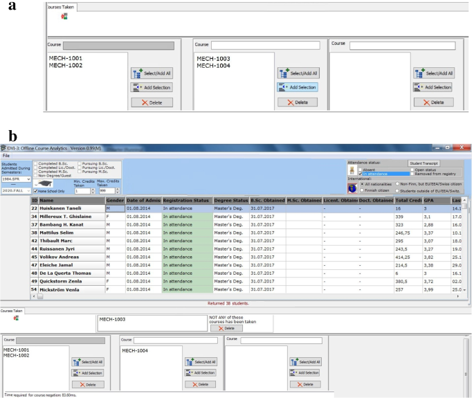

  

  The final incremental steps for the OVI-3 query in Section 4.3. (All names and dates are fictitious). a A query that specifies that either course ‘MECH-A1001’ or ‘MECH-1002’ needs to have been taken in addition to course ‘MECH-1003’ or ‘MECH-1004’. A third, empty course requirement box has appeared in case the user would like to enter further course restrictions to form a conjunction (be ‘ANDed’) with the two leftmost course restriction boxes. b The user has, through a right mouse button click, changed the status of course ‘MECH-1003’ to not-taken. The query therefore stipulates that in addition to course ‘MECH-1004’, students must have passed either course ‘MECH-1001’ or ‘MECH-1002’ and must not have taken course ‘MECH-1003’

  Set S₂ is now updated to students (or rather their student IDs) who took either course ‘MECH-1001’ or ‘MECH-1002’ (or both) and who took either course ‘MECH-1003’ or ‘MECH-1004’ (or both), as shown in Steps 8 and 9 in Algorithm 1. This is achieved by first taking the set of students who took either ‘MECH-1003’ or ‘MECH-1004’ and then taking its intersection with the previous set S₂. We note that when there are three or more course boxes involved, we can compute the S₂ set in steps through binary set intersections or in a single operation that involves all sets (Culpepper and Moffat, 2007). OVI-3 uses the latter approach, and assuming a case with three adjacent course boxes defined, OVI-3 will determine the course box with the least number of elements (i.e., the smallest number of course IDs), say C_j, and then proceed to build the set S₂ by including only those students in course box C_j who also appear in the other key fragment files containing values for α_prim related to the other two course boxes. The restriction for step 4 was completed in just 53.9ms (Table 4).

• Step 5 of the query: placing the negation In the final step (which required 80.4ms as indicated in Table 4), the restriction for course ‘MECH-1003’ is changed from being taken to not being taken by selecting course restriction ‘MECH-1003’, and then pressing the right-mouse button, upon which restriction ‘MECH-1003’ moves into a separate negation area. The final query is shown in Fig. 2b.

  The set S₂ now gets updated to contain only students who have not taken course ‘MECH-1003’ by subtracting from set S₂ those students’ IDs who took course ‘MECH-1003’. These are Steps 10 and 11 in Algorithm 1.

  There is a clear benefit in requiring the user to define a negated restriction by first specifying it in a positive (non-negated) format. This way, when the restriction gets changed into a negation, it is highly likely that the key fragment file associated with the restriction (i.e., values for α_prim, or the student IDs in this case) is going to be found in the cache. Reading the data from cache rather than from slower main memory naturally reduces the query retrieval time (Morfonios & Ioannidis, 2008).

4.6 A comparison of running queries using OVI-3 and an SQL-database

We now compare the performance of the SQL query in Listing 4 to its equivalent OVI-3 query in Section 4.3, which is actually query Q₅ in Table 5. In addition, several other queries (denoted Q₁ to Q₄ and Q₆) tested using both OVI-3 and an equivalent SQL query are shown in Table 5. Note how query Q₃, which only contains a negation, is orders of magnitude faster when using DBI.

Table 5 The total times required to run seven different queries operating on the same data via an SQL query and the equivalent OVI-3 approach

4.6.1 Cost comparison for an anti-join

We next compute the theoretical cost of an anti-join query using the OVI-3 approach and an equivalent SQL-based query. The hypothetical query finds those students who have not taken course ‘MECH-1001’, with the assumption that 256 students have taken that course. It involves two tables, of which R, the larger (1024000 rows), stands for CoursesTaken, while the smaller table S (124000 rows), stands for Students. We denote those 256 students who took course ‘MECH-1001’ through the set $S^{\prime }$, so that $R-S^{\prime }$ is the query’s answer set. We neglect the cost of writing the final answer set to disk and assume a blocking factor of 64 rows per data page.

For the database server side, we assume a text-book approach as in Molina et al. (2009) with a two pass set difference, requiring two block accesses for partitioning and one for the actual set difference, amounting to a query cost $C[_{\text {SQL}}] = 3B(R) + 3B(S^{\prime })$. Substituting, we get B(R) = 1024000/64 = 16000 and $B(S^{\prime })=(124000-256)/64 = 1994$, so the query cost C[_SQL] = 48000 + 5982 = 53982 I/O blocks. Assuming an average access disk time of 8ms per block, 53982 ∗8ms≈ 432s. Little wonder then, that when a similar query (with a much larger number of tables and attributes as the one described here) was run in the Oracle SQL-server, it took about 1h to complete (Query Q₃ in Table 5).

$$\begin{array}{@{}rcl@{}} C_{\text{{OVI-3}}} = h_{R} + {F}_{dir(\text{`MECH-1001'})} + {antijoin}_{\text{(InMemory)}} \end{array}$$

(2)

As for OVI-3, we assume that the DBI technique is implemented via a file management system that uses the B⁺-tree (used with Windows ReFs or NTFS). We allow for 1 billion entries in the disk volume used in the DBI, so a B⁺-tree with height h_R = 5 suffices. The cost for the OVI-3 approach, (2) is the sum of three parts, namely, (1) using DBI to locate the folder corresponding to course ‘MECH-1001’, (2) reading from that folder the contents of the key fragment file F containing values for α_prim (the set $S^{\prime }$), and finally (3), obtaining the result set by subtracting from the primary value store the set $S^{\prime }$. This last step is a memory operation that is assumed never to exceed 0.2s.

The size of file F is assumed to be 1kB (256 ∗4B) where 4B is the key size. Being clearly less than the block size 4kB, the key fragment file can thus be read with a single disk access. Again using an access time of 8ms and assuming 200ms for the memory operation, the cost C_OVI-3 is the sum of the previous parts (1) and (2): (5 + 1) ∗ 8ms + 200ms which translates to 248ms. The measured time for a similar query Q₃ in Table 5, is 2.67s and clearly much larger, due to the fact that negation in OVI-3 occurs in parts (preceded by a non-negated part).

When using OVI-3 to express a negation not A, it will always be immediately preceded by its non-negated restriction A. Thus when computing the negation, the non-negated part A can be assumed to be in memory while the set of all primary keys α_prim always resides in memory. The cost of a negated expression for OVI-3 with respect to its corresponding non-negated expression is thus merely an additional memory access rather than disk access. Computing the ratio for the SQL query costs (measured time over computed time) gives 3604s/ 432s ≈ 8.3 while the similar ratio for the OVI-3-query costs (measured over computed) yields 2.67s / 0.248s ≈ 10.8. This rather minor discrepancy between these two ratios (8.3 and 10.8) supports the notion that the computed costs for both the SQL and the OVI-3 approach are valid.

5 Conclusions

The four presented approaches used with OVI-3, namely (1) DBI, (2) viewpoints, (3) incremental querying and (4) very late materialization are certainly not revolutionary, but when used together, they do allow for efficient handling of primal joins and anti-joins. Incremental querying helps in avoiding unnecessary complex joins, since a new result set gets evaluated as soon as there is a change in the query definition.

Since most OLAP queries can be considered to be essentially ad-hoc, introducing incremental querying into the OVI-3 VQS proved very helpful. The incremental query technique does not fit well into a database server with SQL queries. For instance in VQS SIEUFERD (Bakke and Karger, 2016), the authors provided users with an impression of incremental querying rather than an actual implementation of it.

We did not use a data warehousing approach since the original data for OVI-3 already resided in a relational database. The option of configuring and setting up a big data platform such as SQL-on-Hadoop System (Alavi et al., 2014) was deemed too costly, and querying in the cloud was not an option due to university policy on sensitive data. Moreover, big data platforms are not without their challenges, often providing indexes only for the primary key (Agrawal et al., 2018).

Although OVI-3 is a novel query application that was in test use by three academic counsellors for under a year, it handled their analytical query needs at impressive speeds. The DBI scheme, together with the incremental query approach, truly encourages users to explore data, since each query will, in most cases, terminate well within one second.

References

Abadi, D.J., Madden, S.R., & Hachem, N. (2008). Column-stores vs. row-stores: How different are they really? . In Proceedings of the 2008 ACM SIGMOD International Conference on Management of Data (pp. 967–980). ACM.
Agrawal, D., Chawla, S., Contreras-Rojas, B., & et al. (2018). RHEEM: Enabling Cross-platform data processing: May the big data be with you!. Proceedings of the VLDB Endowment, 11(11), 1414–1427. https://doi.org/10.14778/3236187.3236195.
Ahlberg, C., & Shneiderman, B. (1994). Visual information seeking: Tight coupling of dynamic query filters with starfield displays. In Proceedings of the SIGCHI Conference on Human Factors in Computing Systems (pp. 313–317). ACM.
Ahmed, T., Pedersen, T.B., & Lu, H. (2013). A data warehouse solution for analyzing RFID-based baggage tracking data. In Proceedings of the 2013 IEEE 14th International Conference on Mobile Data Management (pp. 283–292). Washington, DC: IEEE Computer Society.
Alavi, Z., Zhou, L., Powers, J., & et al. (2014). RASP-QS: Efficient And confidential query services in the cloud. Proceedings of the VLDB Endowment, 7(13), 1685–1688.
Atserias, A., Dawar, A., & Kolaitis, P.G. (2006). On preservation under homomorphisms and unions of conjunctive queries. Journal of the ACM, 53(2), 208–237. https://doi.org/10.1145/1131342.1131344.
Bakke, E., & Karger, D.R. (2016). Expressive query construction through direct manipulation of nested relational results. In Proceedings of the 2016 International Conference on Management of Data (pp. 1377–1392). ACM.
Bárány, V, ten Cate, B., & Otto, M. (2012). Queries with guarded negation. Proceedings of the VLDB Endowment, 5(11), 1328–1339. https://doi.org/10.14778/2350229.2350250.
Bellatreche, L., & Boukhalfa, K. (2005). An evolutionary approach to schema partitioning selection in a data warehouse. In Proceedings of the 7th International Conference on Data Warehousing and Knowledge Discovery (pp. 115–125). Springer. https://doi.org/10.1007/11546849_12
Benzi, F., Maio, D., & Rizzi, S. (1996). Visionary: A visual query language based on the user viewpoint approach. In J. Kennedy P. Barclay (Eds.) Proceedings of the 3rd International Workshop on Interfaces to Databases, 8-10 July 1996 (pp. 6–1–6–13). Edinburgh, IDS-3: Springer, Napier University.
Blasgen, M.W., & Eswaran, K.P. (1977). Storage and access in relational data bases. IBM Systems Journal, 16(4), 363–377.
Bouchez, A. (2010). mORMot Open Source Benchmarks. https://synopse.info/forum/viewtopic.php?pid=1011, [Online; accessed 09-May-2022].
Bouchez, A. (2018). Synopse mORMot Framework v.1.18. https://synopse.info/files/html/Synopse18.html, [Online; accessed 7-Jan-2018].
Catarci, T., Costabile, M.F., Levialdi, S., & et al. (1997). Visual query systems for databases: a survey. Journal of Visual Languages and Computing, 8, 215–260.
Ceri, S., Gottlob, G., & Tanca, L. (1989). What you always wanted to know about datalog (and never dared to ask). IEEE Transactions on Knowledge and Data Engineering, 1(1), 146–166. https://doi.org/10.1109/69.43410.
Culpepper, J.S., & Moffat, A. (2007). Compact set representation for information retrieval. In Proceedings of the 14th International Conference on String Processing and Information Retrieval (pp. 137–148). Springer. https://doi.org/10.1007/978-3-540-75530-2_13
Derthick, M., Harrison, J., Moore, A., & et al. (1999). Efficient multi-object dynamic query histograms. In Proceedings of the 1999 IEEE Symposium on Information Visualization (pp. 84–91). IEEE.
Eichmann, P., Zgraggen, E., Binnig, C., & et al. (2020). Idebench: A benchmark for interactive data exploration. In Proceedings of the 2020 ACM SIGMOD International Conference on Management of Data (pp. 1555–1569).
El-Mahgary, S., & Soisalon-Soininen, E. (2015). A form-based query interface for complex queries. Journal of Visual Languages and Computing, 29(C), 15–53.
Embarcadero Technologies. (2018). Delphi Homepage. https://www.embarcadero.com/products/delphi, [Online; accessed 4-Jan-2018].
Gessert, F., Wingerath, W., Friedrich, S., & et al. (2017). NoSQL database systems: a survey and decision guidance. Computer Science - Research and Development, 32, 353–365. https://doi.org/10.1007/s00450-016-0334-3.
Goodman, J.R. (1980). An investigation of multiprocessor structures and algorithms for data base management. PhD thesis, University of California, Berkeley.
Greco, S., & Molinaro, C. (2016). In Z. Meral Özsoyoğlu (Ed.) Datalog and Logic Databases. Synthesis Lectures on Data Management. https://doi.org/10.2200/S00648ED1V01Y201505DTM041. Morgan & Claypool Publishers.
Gutiérrez-Basulto, V, Ibáñez-garcía, Y., Kontchakovc, R., & et al. (2015). Queries with negation and inequalities over lightweight ontologies. Journal of Web Semantics, 35, 184–202.
Hamdi, M., Yu, F., Alswedani, S., & et al. (2017). An efficient data structure for fast join query processing. In IEEE Technically sponsored future technologies conference (FTC) 2017 (pp. 483–492).
Idreos, S., Kersten, M.L., & Manegold, S. (2009). Self-organizing tuple reconstruction in column-stores. In Proceedings of the 2009 ACM SIGMOD International Conference on Management of Data (pp. 297–308). ACM.
Ilyas, I.F., Aref, W.G., & Elmagarmid, A.K. (2004). Supporting top-k join queries in relational databases. The VLDB Journal, 13(3), 207–221.
Larson, J.A. (1986). A visual approach to browsing in a database environment. Computer, 19(6), 62–71. https://doi.org/10.1109/MC.1986.1663255.
Lazarus. (2018). Lazarus homepage. https://www.lazarus-ide.org/.
Li, Z., & Ross, K.A. (1999). Fast joins using join indices. The VLDB Journal, 8(1), 1–24. https://doi.org/10.1007/s007780050071.
Liu, Z., & Heer, J. (2014). The effects of interactive latency on exploratory visual analysis. IEEE Transactions on Visualization and Computer Graphics, 20 (12), 2122–2131. https://doi.org/10.1109/TVCG.2014.2346452.
Lo, A., Özyer, T., Kianmehr, K., & et al. (2010). VIREX and VRXQuery: Interactive approach for visual querying of relational databases to produce XML. Journal of Intelligent Information Systems, 35(1), 21–49. https://doi.org/10.1007/s10844-009-0087-6.
Minock, M. (2003). Knowledge representation using schema tuple queries. In Proc. of KRDB 2003, Hamburg, Germany, September 15-16, 2003, Vol. 79. IEEE Computer Society Press.
Mishra, P., & Eich, M.H. (1992). Join processing in relational databases. ACM Computing Surveys, 24(1), 63–113. https://doi.org/10.1145/128762.128764.
Molina, H.G., Ullman, J.D., & Widom, J. (2009). Database Systems, 2nd edn. Pearson Prentice Hall.
Morfonios, K., & Ioannidis, Y. (2008). Supporting the data cube lifecycle: the power of ROLAP. The VLDB Journal, 17(4), 729–764.
Nandi, A., & Jagadish, H.V. (2011). Guided interaction: Rethinking the query-result paradigm. PVLDB, 4(12), 1466–1469.
Schweikardt, N., Schwentick, T., & Segoufin, L. (2010). Database Theory: Query Languages, 2nd edn., CRC Press, pp 1–48.
Sippu, S., & Soisalon-Soininen, E. (1996). An analysis of magic sets and related optimization strategies for logic queries. Journal of the ACM, 43(6), 1046–1088. https://doi.org/10.1145/235809.235814.
Soylu, A., Giese, M., Jiménez-Ruiz, E., & et al. (2016). Experiencing optiquevqs: A multi-paradigm and ontology-based visual query system for end users. Universal Access in the Information Society, 15, 129–152.
Stolte, C., Tang, D., & Hanrahan, P. (2002). Polaris: A system for query, analysis, and visualization of multidimensional relational databases. IEEE Transactions on Visualization and Computer Graphics, 8(1), 52–65.
Stonebraker, M., Abadi, D.J., Batkin, A., & et al. (2005). C-store: A column-oriented DBMS. In Proceedings of the 31st International Conference on Very Large Data Bases. VLDB Endowment (pp. 553–564).
Tanin, E., Beigel, R., & Shneiderman, B. (1996). Incremental data structures and algorithms for dynamic query interfaces. SIGMOD Rec, 25(4), 21–24.
Acknowledgements
We are grateful for Academy of Finland’s grants as listed below in Funding. Besides the academic counsellors who tested OVI-3, we also gratefully acknowledge the following key people at Aalto University’s School of Engineering for their kind support for OVI-3Footnote 6: Ms. Soile Koukkari (Development Manager), Mr. Harri Långstedt (Coordinator) and Dr. Kirsi Virrantaus (Vice-Dean).
Funding
Open Access funding provided by Aalto University. Academy of Finland, grants no 295908 (Techniques for efficient processing of big data), no 272195 (CoE-LaSR) and no 293389 (Combat).
Author information
Authors and Affiliations
Contributions
S.E. developed the system and wrote most of the paper. E.S-S., P.O. and P.R made substantial contributions towards the clarity of the paper’s presentation. Authors P.R and H.H contributed towards the design of the VQS’s interface. All authors reviewed and commented on the manuscript.
Corresponding author
Ethics declarations
Human and animal Ethics
Not Applicable.
Ethics approval and consent to participate
The included screenshots refer to imaginary students. There are no references to real life persons or to their opinions.
Consent for publication
There are no references or identifiable details to any participants in this work.
Competing interests
The authors have no conflicts of interest to declare that are relevant to the content of this article.
Additional information
Publisher’s note
Springer Nature remains neutral with regard to jurisdictional claims in published maps and institutional affiliations.
Rights and permissions
Open Access This article is licensed under a Creative Commons Attribution 4.0 International License, which permits use, sharing, adaptation, distribution and reproduction in any medium or format, as long as you give appropriate credit to the original author(s) and the source, provide a link to the Creative Commons licence, and indicate if changes were made. The images or other third party material in this article are included in the article's Creative Commons licence, unless indicated otherwise in a credit line to the material. If material is not included in the article's Creative Commons licence and your intended use is not permitted by statutory regulation or exceeds the permitted use, you will need to obtain permission directly from the copyright holder. To view a copy of this licence, visit http://creativecommons.org/licenses/by/4.0/.
About this article
Cite this article
El-Mahgary, S., Soisalon-Soininen, E., Orponen, P. et al. OVI-3: A NoSQL visual query system supporting efficient anti-joins. J Intell Inf Syst 60, 777–801 (2023). https://doi.org/10.1007/s10844-022-00742-4
Received:
Revised:
Accepted:
Published:
Issue Date:
DOI: https://doi.org/10.1007/s10844-022-00742-4