
Abstract
This paper investigates the relationship between State aid measures, as defined by Article 107 of the Treaty on the Functioning of the European Union (TFEU), and firm performance in terms of total factor productivity (TFP). Under imperfect capital markets, firms might encounter difficulties in accessing sufficient resources to fund their optimal investment plans. The main focus of this paper lies in establishing whether State aid alleviates a firm from such constraints, and thereby enhances its productivity. To this end, we include all State aid cases that were active in Belgian manufacturing between 2003 and 2012. To determine the effects of State aid and financing constraints on performance, we first estimate TFP and classify firms according to their financial health in the absence of aid. The main results confirm the hypothesis, but when allowing for firm heterogeneity, a mitigating role for State aid is only present for initially well-performing firms.
1 Introduction
Although the Modigliani-Miller theorem tells us that the financial structure of firms and financial policy are irrelevant for a firm’s investment decisions (Modigliani and Miller 1958), investment can be substantially hampered by the existence of financial constraints. Capital markets might fail to efficiently allocate resources for the firm to develop optimally. Due to informational asymmetries and/or a lack of substantial tangible collateral, a firm can experience difficulties in obtaining external funding for its projects. Under innovational rivalry, investment will be slowed down and projects can be abandoned when a firm needs to rely on insufficient availability of internal fundingFootnote 1 (Kamien and Schwartz 1978).
Alongside market failures due to the positive externalities of R&D investment resulting in suboptimal investment levels, financial constraints resulting from imperfect capital markets are justifications for government intervention. A large body of literature evaluates public R&D policies in light of the former type of market failures.Footnote 2 The link between financial constraints and public intervention in the form of State aid, however, seems to be less emphasized, with the notable exceptions of Czarnitzki (2006) and Hyytinen and Toivanen (2005). They find evidence in support of governmental intervention alleviating the constraints resulting from capital market imperfections. This paper differs from these studies in that we include all firms rather than focusing on small and medium-sized enterprises (SMEs).
The purpose of the present paper is to establish the relationship between State aid and firm performance and particularly, the role of the firm’s financial health status therein. This paper differs from previous studies as we do not focus on R&D subsidies per se, but the effects of financial constraints and State aid regardless of the goal of the measure. As a measure of R&D investment is not included in our dataset, we concentrate on performance in terms of total factor productivity. To this end, we use all Belgian State aid cases in manufacturing that were active between 2003 and 2012 and link them to firm-level financial data. As it is of particular interest whether aid measures help firms overcome some of their financing constraints, we require a measure of financial constraints in the absence of aid. To overcome this missing data problem, firms are classified according to their financial health status using nearest neighbor predictive discriminant analysis. The predictors of this model include firm characteristics such as age and size as well as sector and regional indicators. As a final step in the analysis, we estimate the joint effects of State aid and financing constraints on the performance of the firm.
Our results show that State aid is more effective in terms of productivity gain when granted to financially constrained firms. This suggests that State aid can relieve a firm of its financial burden and induce investment that would otherwise not have taken place. When allowing for firm heterogeneity, this beneficial effect is only present when the firm was already performing well. In addition, we find that small firms benefit relatively more from State aid than larger firms. However, we find no evidence that age matters.
The next section gives a brief overview of the relevant literature. Sections 3 and 4 describe the data and the estimation strategy, as well as some key summary statistics. The results are presented in section 5 and section 6 provides some robustness checks. The last section contains the conclusions and some suggestions for future research possibilities.
2 Brief Overview of the Literature
There exists a wide consensus on the devastating effect of financial constraints on investment and innovation, as these have been shown to have an important impact on a firm’s investment decisions. For a firm to conduct the necessary investment towards innovation, it must have access to a source of financing, either internal through its current profits and accumulated funds or external through capital markets. However, due to a lack of tangible collateral and informational asymmetries with external investors, a firm might face a binding cash constraint when it is not able to finance its projects with its own resources. In a seminal work, Kamien and Schwartz (1978) show that such a binding constraint can not only slow down the pace of development, but also reduce the acceptability of R&D projects all together.
A large body of empirical literature thereafter examines the existence of financial constraints and their relationship with investment, which is considered one of the main driving forces behind innovation and ultimately firm performance. In their survey on financial constraints, Carreira and Silva (2010) summarize and discuss the main findings resulting from these studies with several stylized facts. As an extensive treatment of this literature is beyond the scope of this paper, we highlight three of their main findings. Firm dynamics are altered in the absence of sufficient internal funding, both in terms of efficient entry of firms (see e.g. Aghion et al. (2007)), and in terms of firm survival (see e.g. Musso and Schiavo (2008)). Several studies show that the likelihood of innovation decreases as the firm faces financial constraints (e.g. Savignac (2008)).
As the emergence of financial constraints is mainly due to market failures such as information asymmetries and moral hazard issues,Footnote 3 there is scope for government intervention to increase the market’s efficiency. In fact, one of the main objectives of European State aid policy consists of enhancing growth and innovation by designing it in such a way as to sustain competitive markets. Improving the functioning of some markets may improve competitive dynamics, thereby inducing economic growth (Kleiner 2005). The general principle for assessing the compatibility of a particular State aid case consists of a balancing test which considers the trade-off between the positive and negative effects of the measure (such as distortion of competition, direct cost of the subsidy, and the deadweight loss arising from the distortive effect of taxation) (Friederiszick et al. 2006).
As one of the primary objectives of European State aid control is to prevent any distortion of competition or trade between the Member States, part of the literature on State aid policy focuses on the effect on market competition.Footnote 4 Buts and Jegers (2013) show that State aid results in higher market shares for the aid-receiving firms, as well as an increase in market concentration, using Belgian firm-level data between 2005 and 2008. Aghion et al. (2015) include the growth objective in their analysis on industrial policy and competition and find evidence that sectoral policy instruments are associated with higher total factor productivity in a more competitive-friendly environment. By distorting the natural order of the competitive environment, the risk arises that low productive firms are kept in the market at the expense of better performing ones. In a recent line of research, it is shown that the existence of so-called “zombie” firmsFootnote 5 reduces the profits for healthy firms, discouraging their entry and investment through congestion of the market (see e.g. Caballero et al. (2008) on Japan, and Tan et al. (2016) on China). Within the OECD, the prevalence of and resources sunk into zombie firms have risen since the mid-2000s, leading to a decline in potential output growth (McGowan et al. 2017).
Ex-post evaluation of different types of State aid schemes is used to determine the effectiveness of the measures. In a cross-country analysis, Gual and Jódar-Rosell (2006) study the impact of vertical industrial policiesFootnote 6 on Multifactor Productivity Growth in the manufacturing sectors. Although these types of measures are considered the most distortive in terms of competition, vertical State aid measures contribute positively to productivity growth. In light of the financial crisis in Europe, Grigolon et al. (2016) show that scrapping schemesFootnote 7 in the car industry contributed to the stabilization of total car sales and generated environmental benefits due to the substitution of more fuel efficient cars. More recently, Heim et al. (2017) find that Rescue and Restructuring aidFootnote 8 increases firms’ probability of survival and improves their financial viability. A large part of the literature on public support, however, is concerned with the impact on R&D and investment as these are considered the building blocks of economic growth.
The impact of public policies on R&D has been reviewed by Becker (2015). She concludes that public R&D policies succeed in stimulating private R&D, irrespective of the instrument used (tax credit, subsidies…). Small firms tend to benefit more from these policies and are more likely to start investing in R&D as they are more likely to be constrained. However, as stated in Hall (2002) not many studies take into account the financial constraints argument as a justification for public policies. In particular, Czarnitzki (2006) compares the impact of financial constraints on German SMEs using the differences in public policy between East and West Germany. He finds that firms are not only sensitive to both internal and external funding constraints, but their R&D expenditure is raised by public support. Interestingly, this result does not hold for East German firms that benefit on a more structural basis from public support. Hyytinen and Toivanen (2005) show that public support disproportionally helps Finnish SMEs in sectors that are dependent on external funding.
Although the ex-post evaluation of different types of State aid has been most frequently visited in the light of R&D public policies, it is interesting to see whether State aid, irrespective of its goal, would still generate a positive impact on firms’ productivity through the alleviation of financing constraints. As far as we are aware, this is the first paper to look at a more general link between European State aid, financing constraints, and total factor productivity.
3 Data and Variable Definitions
3.1 Data Description
To examine whether State aid can boost a firm’s productivity by alleviating an existing financial constraint, we extract information from 3 sources. Our primary data source is Belfirst, a commercial database published by Bureau Van Dijk, which contains the income statements for all Belgian companies. We retrieve information on all Belgian firms active in manufacturing for which information is available on value added, employment, material costs, employment costs, tangible fixed assets, and total assets during the time period 2003 to 2012. To avoid outliers driving the results, the bottom and top percentile observations are dropped. After data cleaning, we are left with 9255 firms that are primarily active in manufacturing. Almost half of these firms (4389) are multiproduct firms, measured at the 5-digit NACE code level.
Secondly, we use a comprehensive database of State aid cases that have been the object of a Commission decision from 2000 onwards, which is freely available from the European Commission. We focus on all cases that apply to manufacturing firms and that were “active” between 2003 and 2012. In order to identify these cases, we complement this database with information published in the Official Journal of the European Union (OJEU). In the final dataset we identified 114 State aid cases, of which 51 cases can be directly linked to 88 receiving firms. The remaining 63 cases have information on either the sectorFootnote 9 (NACE Rev.2) or the region levelFootnote 10 (indicated by NUTS) or a combination. Unfortunately, 23 additional cases are rather general measures for which is not clear which firms can benefit from them. Note that a State aid case can be applicable to multiple sectors and/or regions. For the empirical analysis, we only include the State aid cases for which at least 4-digit sector level information is available.
Although State aid is generally prohibited in the European Union,Footnote 11 Member States are allowed to intervene in the market, by e.g. providing subsidies, if the aid is justified by reasons of general economic interest. Before they can implement the desired measure, Member States are obliged to notify the European Commission who will decide whether or not the aid is compatible with the internal market following the exemptions stipulated in the TFEU.Footnote 12 The number of cases initiated varies greatly by year, as well as across sectors and regions. Figure 1 shows the evolution by the year of notification between 1999 and 2013. We can distinguish two clear waves, in the years 2003 and 2004 and at the start of the financial crisis in 2008. Note, however, that the low numbers of cases in 1999 and the latest years are due to the selection of cases that were active within our sample of firm-level data. Table 1 provides an overview of the number of cases in relation to the number of firms in each sector.
As all State aid, by definition, provides an economic (and potentially financial) advantage to the recipient, we include all cases irrespective of the goal (objectives) and the instrument of the measure. The objectives form the legal basis for the Member States to grant State aid. Table 2 gives the number (percentage) of cases by objective and by instrument. On average, a State aid measure lasts for approximately 3.5 years, although most cases are “one-shot” direct grants. Panel A of Table 3 presents summary statistics on some key variables, i.e. size of the firm (in terms of total assets and employment), age of the firm, and the productivity level. The differences between State aid and Non-State aid firms are negligible. From the distribution of all State aid firms across the quintiles of the initial values of the same variables in Panel B, we learn that large, old, and more productive firms attract more State aid. Note, however, that under the De Minimis Regulation, small amounts of aid do not need to be notified to the European Commission.
3.2 Variable Definitions
The goal of this paper is to establish whether State aid can enhance the performance of a firm through the relief of some financial barrier(s). In order to do so, we need measures of both firms’ performance and financing constraints in the absence of State aid. Our independent variable will be obtained by estimation of total factor productivity (TFP) using Wooldrigde (2009)’s adaptation of the Levinsohn and Petrin (2003) estimator. To classify the firms according to their financial health, we rely on nearest neighbor predictive discriminant analysis.
3.2.1 Dependent Variable: Total Factor Productivity
To account for the well-known selection and simultaneity problem when estimating production functions, we rely on the insights provided by Olley and Pakes (1996) and Levinsohn and Petrin (2003), hereafter referred to as OP and LP, respectively. To cover the Ackerberg et al. (2006) critique, we follow Wooldrigde (2009) by using a one-step GMM version of LP estimator. This methodology has the additional advantage that it does not require bootstrapping to retrieve robust standard errors. The estimation procedure is repeated for every sector, measured at the 2-digit NACE level. To account for price changes, all variables are deflated using appropriate deflators obtained from the OECD. All estimations include year dummies.
We consider a value added Cobb-Douglas production function \( {Y}_{it}=\left({K}_{it}^{\alpha_K}{L}_{it}^{\alpha_L}\right){e}^{\omega_{it}+{\eta}_{it}} \) where Yit, Kit, Lit respectively represent value added, capital input, and labor. The error term ηit is usually thought of as shocks to production or productivity unobservable by firms and thereby uncorrelated to input decisions such as deviations from expected breakdown or measurement error in the output variable. For our analysis, the variable of interest in this equation is ωit which is usually referred to as total factor productivity or “unobserved productivity”. It represents shocks that are observed or predictable for the firm when making input choices but that are unknown to the econometrician. The estimating equation for a single product firm is given by (in logs):
where the lower-case letters indicate the logarithms of the respective upper-case variables. We assume that the productivity process evolves according to a first order Markov process given by \( p\left({\omega}_{i t+1}|{\left\{{\omega}_{i\tau}\right\}}_{\tau =0}^t,{I}_{i t}\right)=p\left({\omega}_{i t+1}|{\omega}_{i t}\right) \) where Iit is the firm’s entire information set at time t.
The estimation procedure consists of two stages, where the first stage separates the unobserved productivity term, ωit from the error term, ηit. We use the firm’s choice of intermediate inputs (materials) to proxy for unobserved productivity. Under the assumption that a firm’s material input demand function is monotonically increasing in ωit, we can rewrite the estimating equation as follows:
where ϕt(kit, lit, mit) = βllit + βkkit + ht(kit, lit, mit) in which the last term is the inverse material demand function. The productivity process is given by a law of motion represented by ωit = g(ωit − 1) + ξit, where g is some function and ξit is usually interpreted as innovation in the production process that is unexpected to the firm. By construction, this innovation term is uncorrelated with kit and lit − 1 as both are contained in the firm’s information set at time t.Footnote 13 This leads to the second stage equation:
where lit − 1 is used as an instrument for lit. As noted before, both stages are estimated in a one-step GMM procedure known as the Wooldridge-Levinsohn-Petrin estimator.
Multisector, −Segment, and -Product Firms
Our data has the special feature that we know all sectors in which a firm is active.Footnote 14 There are 862 firms that produce products which are categorized in different sectors within manufacturing. The financial data are, however, known only at the firm level. As we do not know how much of the input choices are attributed to each sector, we apply a proportionality principle based on the number of products produced by the firm. Denote the total number of products for a firm i by Ji and within a sector s and Jis. Adjust the dependent variable and the independent variables in the following manner:
where f = {k, l, mc}.
In addition, we wish to account for the presence of multiproduct firms, measured at the 5-digit NACE code level. Under the standard assumption of identical production functions across products produced, controlling for the number of products suffices to introduce multiproduct firms within this framework. All estimations also include segment dummies, accounting for differences between all segments within the sector, and include the information on firms that are active in more than one segment (De Loecker 2011).
The results of this estimation procedure are presented in Table 4. For the subsequent analysis, we use the coefficient estimates from Column (d). An estimated measure for TFP is then obtained by
3.2.2 Classification Method
In order to classify firms according to their financial status, we require some adequate measure of financial constraints which has proven to be a difficult task. We follow and adapt the methodology of Cleary (1999) by classifying firms into groups according to a financial constraint index. This index is determined by non-parametric predictive discriminant analysis, in particular using the nearest neighbor, i.e. the firm that is the most similar in terms of a number of characteristics which are associated with the existence of financial constraints. There are two main advantages to this methodology. Primarily, firm classification is allowed to change over time to reflect that a firm’s financial status can evolve over time. Secondly, this methodology takes into account an entire profile of characteristics instead of relying on a single proxy variable.
In this paper, we rely on the current ratio as a segmenting variable determining a firm’s financial health and use predictive nearest neighbor discriminant analysis to classify all firms. The working capital ratio, also called the current ratio (CR), indicates whether a firm is able to fund its current liabilities with its current assets. Generally, a firm with a CR exceeding 1.2 is considered to be financially healthy. However, there may be substantial differences between sectors of what is considered good practice. Therefore, we define a firm to be financially constrained if the CRjt is below 60% of the median value in sector j (defined at the 2-digit level) at time t. For the moment, we disregard that a too high CR is not necessarily a sign of good investment management. To avoid outliers driving the results, the observations for which the CR exceeds 10 are excluded.
Table 5 provides the summary statistics of the current ratio by sector. There are large differences in the average value of the current ratio, with a range from 1.46 in Food Manufacturing to 2.003 in Manufacturing of Rubber and Plastics. These differences remain valid when examining the median.Footnote 15 Although the defined cut-off value is the lowest for Food Manufacturing (sector 10), almost 21% of the firms score below this value. The least constrained sector is “Machinery and Equipment” (sector 28). Over the entire sample, 14.6% of the firms are categorized as being financially constrained. Note that only the firms that did not receive State aid are included in this table. Our measure is rather conservative since the cut-off value is well below the “healthy” 1.2.
We divide all firms into three groups: (i) financially constrained firms that did not receive State aid (FC), (ii) firms with a high current ratio that did not receive State aid (NFC), (iii) firms that received State aid (SA). For the last group, there is a “missing data problem”, i.e. we cannot observe whether a firm would have experienced financial difficulties without the aid measure. These observations are therefore not used to determine the discriminant specification but are assigned to a group.
Panel A of Table 7 reports summary statistics for a group of variables that are usually associated with financial constraints. These variables can be roughly categorized in the following way: firm characteristics such as age and size of the firm,Footnote 16 demand indicators, liquidity availability, access to external funding, and market structure. In line with the literature, FC firms are younger and smaller. In the first group 14.4% of the firms are younger than 5 years whereas in group 2 only 6.44% are younger. On average, the State aid-receiving firm is older and about average in size. There are no big differences in the EBITDA measure but based on the profit margin NFC firms are more profitable, as expected. They also incur higher debt ratios and experience lower sales growth. Overall, firms have a 16% probability of being in a period of financial distress. The SA firms are at slightly higher risk with 18%. Panel B of Table 7 presents the number of firms for each year by group.
Discriminant analysis uses a number of variables that are likely to influence characterization of a firm in one of the two mutually exclusive groups of interest. The hypothesis is that these variables will enable us to predict whether firms are financially constrained. The nearest neighbor classification of Fix and Hodges (1951) is the earliest and most intuitive nonparametric classification method. In particular, an observation (firm-year) is represented by a vector of characteristics, xi. For each observation, nni is defined as the nearest neighbor if the squared Mahalanobis distance \( d\left(\boldsymbol{n}{\boldsymbol{n}}_i,\boldsymbol{x}\right)=\underset{j}{\min}\left\{d\left(\boldsymbol{n}{\boldsymbol{n}}_j,\boldsymbol{x}\right)\right\} \). The predicted class of an observation is set equal to the true class of the nearest observation. In addition, we like some measure of the probability of being constrained. For this purpose, we consider the k nearest neighbors and specify the posterior-probability to be constrained as
where k = kFC + kNFC and n = nFC + nNFC represent the number of neighbors considered and the number of observations in the sample, respectively.
As it is important that the predicted classification is not influenced by State aid, the predictors included should be unlikely to change (rapidly) with State aid. This leaves us with a small subset of potential predictors, namely the age and size of the firm, the number of products produced (as this measure remains stable over the sample), time, region, and sector. To account for differences between sectors, we estimate both the probabilities and group classification by sector and adapt the subset of predictors according to the predictive power. For the multisector firms, a firm is identified as being constrained if it is predicted as such in one of the sectors in which it is active.
4 Estimation Strategy
Our hypothesis states that if a firm experiences some sort of financial barrier, it will be less efficient due to underinvestment. Therefore, the model we want to estimate can be written in reduced form in the following way:
where SAit and FCit are dummy variables indicating, respectively, whether or not the firm was the beneficiary of a State aid measure or experienced some financial constraint. To estimate this model, we use a conditional difference-in-differences estimator. This estimator allows controlling for permanent differences between firms that received State aid or experienced some financial barrier in the time frame of the sample. To avoid severe bias to the estimates, we include controls for time, sector, and region of operation. Since we do not have a direct measure of financial constraints, we use the generated regressor obtained through the prediction method explained above. Although this does not affect consistency of the estimated coefficient under fairly standard assumptions, standard errors are usually invalid (Wooldridge 2002). Thus, standard errors are obtained through bootstrapping where we resample panels rather than observations to account for the longitudinal structure of the data.
The effect of State aid can differ greatly among firms. An important source of heterogeneity in the current setting involves their initial productivity levels. If there exists a natural order to e.g. exit or gain profits according to the potential of the firms, it is likely to be positively correlated with the access to financial means. Hence, β2 in Eq. 7 might overestimate the negative effects of financial constraints on performance. Moreover, in this way, financial constraints might be a “natural” mechanism to punish bad performers. If State aid distorts this natural order, we keep “losers” in the game at the expense of “winners.” A similar problem arises with the State aid variable. If a government’s industrial policy is mainly based on a “picking winners” strategy, the coefficient of State aid (β1) in Eq. 7 will be upwards biased.Footnote 17 To account and control for these differences in initial productivity and examine the potential different outcomes, we adapt the estimation equation as follows:
where lnTFPi0 is the logarithm of the total factor productivity estimate in the first period. We allow for the effect of State aid to be different for financially constrained and/or highly efficient firms.
The crisis years have been different in many perspectives. First of all, it is likely that more State aid measures were issued or differently assessed. Secondly, as the crisis hit suddenly and unexpectedly, firms were not prepared. To account for these different macro-economic circumstances, we repeat the above analysis on a split sample, i.e. before and after 2008.
5 Results
The baseline estimation results for Eq. 7 are presented in Table 8. The first three columns provide some insight on the expected productivity levels conditional on State aid and financing constraints. Indicator variables to control for inherent differences between supported and non-supported, and/or financially constrained and unconstrained firms are included. Column (1) shows that the estimated gross impact of State aid, i.e. the difference in performance between aid-receiving and non-receiving firms, conditional on their financial status, is positive and statistically significant. In line with expectations, financially constrained firms are associated with substantially lower productivity estimates. Of particular interest is β3, the coefficient of the interaction term, SAit ∗ FCit that is expected to be positive if State aid is able to mitigate the negative effects of financing difficulty. Indeed, we find that the beneficial effect of State aid is larger for firms that are in need of some financial assistance. All specifications include time-fixed effects to control for common changes through time. Starting from Column (3), we include additional controls for year-specific differences between SA and non-SA firms.
Column (4) introduces sector dummies whereas column (5) extends further with regional dummies. Productivity estimates can vary widely across sectors due to differences in efficiency potential as well as in propensities to receive State aid across sectors. Governments might be more willing to provide State aid in high-performing sectors leading to an upwards bias of the estimated coefficient β1. As State aid measures can be initiated from several government levels, the probability of receiving aid is likely to differ across geographical locations. We do not expect large differences in decision making over such a short time period but if there are, our estimates still contain some bias. The direction of such a bias, however, is less clear. Conditioning on sectoral and regional differences, we find no statistically significant effect on productivity from granting State aid to firms that have sufficient internal funding. This may be due to several factors, including liquidity hoarding, less efficient use of resources, “crowding-out” effects, and “too big to fail” strategies. However, when a firm has limited internal resources, State aid is associated with an increase in the productivity level completely offsetting the disadvantage resulting from their financing constraints.
As the resilience and dynamics of firms to overcome financial difficulty might substantially change according to macro-economic circumstances, we repeat the estimation for a split sample. Column (6) presents the results for the years 2003 to 2007, and Column (7) involves the estimation for the crisis years. Our conclusions do not alter from the first period to the next.
By estimating Eq. 8, we allow for heterogeneous effects of State aid and financial constraints according to their initial productivity levels. By simply conditioning on these initial levels, the gross impact of State aid becomes statistically insignificant. The same conclusion applies to the interaction term, SAit ∗ FCit. This, however, hides some substantial heterogeneity in the effects of State aid on productivity for firms that differ in their level of technological advances. We expect more productive firms to be more resilient with respect to negative (financial) shocks. If a firm experiences financial difficulty due to bad management, low past profits…, State aid might not be very effective in resolving these issues. However, if a temporary negative shock hits the economy, or a certain sector, State aid might mitigate these shocks for the most resilient firms. We expect firms operating at technological frontiers to be more likely to show that resilience. The same line of reasoning can apply in the case of high-risk investment. If the productivity in the firm is already high, past ideas/investment have already succeeded and the likelihood of success will also be higher. The results presented in the fourth column suggest even stronger implications: if the firm experiences some financial difficulty, the mitigating role of State aid is only present for highly performing firms. Columns (5) & (6) show the results for the split sample. We can confirm these results for the pre-crisis period (Table 9).
Throughout the literature the role of the firm’s size and age on the existence of financial constraints is emphasized. On average, small firms experience more difficulty in obtaining the necessary funds for investment. Large firms might enjoy more internal financing (“deep pockets”) and/or have better access to external sources of liquidity. They benefit from being well-known and having better relations with external investors or lenders (Cohen and Klepper 1996). Several studies show that financial development has disproportionally positive effects for small firms (Aghion et al. 2007; Beck et al. 2005; Rajan and Zingales 1998). Although younger and smaller firms are more likely to be unable to obtain external funding such as a bank loan (Levenson and Willard 2000; Canton et al. 2013), this does not imply the firm’s growth is hampered. In particular, small firms tend to remain small even under better financial conditions (Hurst and Pugsley 2011). Conditional on survival, young firms are usually associated with higher growth rates because they are still on a steep learning curve. In addition, they tend to undertake riskier innovation. The performance benefits from investment in R&D are larger if successful, but they also experience a larger decline in the case of failure (Coad et al. 2016).
To account for the potential different effects expected for small and young firms, we repeat the above analysis on subsamples of such firms. As can be seen from Fig. 3, a large majority of firms can be classified as a Small and Medium-Sized Enterprise (SME). Therefore, we focus on the Micro and Small enterprises with less than 50 employees and turnover below 10 million euro. The results are provided in Tables 10 and 11. Overall, we do not find a statistically significant effect of State aid on firm performance for small firms. For the pre-crisis period, State aid is mitigating the negative effects of financing constraints, but the effect is smaller and significant only at the 10% level. Allowing for firm heterogeneity in terms of initial TFP, we can confirm our previous conclusion, namely well-performing firms that encounter some financial barrier benefit disproportionally from State aid. These results were mainly driven by the pre-crisis period.

NUTS classification for Belgium (3-digit level). This figure presents all the Belgian regions at the NUTS 3-digit level. Source: Eurostat (http://ec.europa.eu/eurostat/documents/3859598/5916917/KS-RA-11-011-EN.PDF, p15-18)

Percentage of firms by size categories. This figure shows the percentage of firms by size categories. The categories are determined following the definitions set out by the European Commission (http://ec.europa.eu/growth/smes/business-friendly-environment/sme-definition_nl): 1. Micro firms (size 1): < 10 employees and < 2 million EUR turnover, 2. Small firms (size 2): < 50 employees and < 10 million EUR turnover, 3. Medium sized firms (size 3): < 250 employees and < 50 million EUR turnover, 4. Large firms (size 4): > 250 employees or > 50 million EUR turnover
Table 12 presents the main results for young firms. In this context, a firm is considered young if its age is below 10 years. The sample used in these regressions includes all firms that were young at the time of the first observation in the dataset. Correcting for common time shocks and permanent differences between supported and non-supported firms, being the beneficiary of a State aid measure is associated with 36.4% higher performance. Even if we control for sector, region, and time-dependent differences, this effect is still 20% and highly statistically significant (Column (6)). Most of the previous conclusions also hold for the group of young firms, although the effects seem to be somewhat larger. In contrast to the entire sample and the small firms, however, the results are now mainly driven by the post-crisis years. This is in line with the literature that suggests that young firms are more likely to be hit disproportionally by (common) negative shocks. Once controlled for initial performance levels, the significance of the State aid effect becomes insignificant (see Table 13). In contrast to the entire sample, this does not seem to hide heterogeneous effects between better and worse performers. This suggests either that State aid for these firms was granted to the “winners,” or that the purposes of State aid for young firms were focused on other goals such as employment or training.
6 Robustness Checks
This section presents several robustness checks in order to verify that the results above are not driven by mere chance. We discuss some concerns and consider various alternatives for our main variables used throughout the analysis.
6.1 Robustness Checks Concerning the Measure of Productivity.
To eliminate price effects, we followed the standard solution of using deflated firm-level added value by an industry-wide producer price index. However, the coefficients of the production function might still be biased if the price error (difference between the industry price index and a firm’s actual price) is correlated with a firm’s input choices (De Loecker 2011) which is known in the literature as omitted price bias. This may lead to an important identification problem regarding the relationship between financing constraints and productivity. Foster et al. (2008) show that small firms often appear to have lower revenue-based productivity simply because they charge lower prices than large firms. On the other hand, financially constrained firms charge lower prices because they produce low quality products (see Fan et al. 2015; Bernini et al. 2015). This, however, does not have to be problematic if quality differences are fully reflected in prices (Syverson 2011). In addition, it should equally be noted that welfare implications of State aid measures are therefore unattainable. In future research, it would be interesting to see whether results fully carry over when using TFPQ rather than TFPR.
To establish some robustness concerning the independent variable, i.e. total factor productivity it is interesting to see whether our results carry over to labor productivity. We define labor productivity as the log-ratio of value added on labor (number of employees):
where Yit and Lit denote, respectively, the real value added and labor of firm i at time t. To obtain the “heterogeneity” results, we include lnLPi0, the logarithm of labor productivity at the first observation. The results are presented in Table 14. All previous obtained results hold but the statistical significance of the coefficients is lower. State aid mitigates the negative effect of financial constraints for highly productive firms only in the first period of the sample (before the crisis), but it is only weakly significant with a p-value of 0.101.
In addition, the initial TFP measure is replaced by a relative measure as the opportunity/possibility for productivity improvements might differ substantially across sectors. We define the variable distanceit as the distance of firm i to the possibility frontier at time t. This frontier is determined by the best performing firm in the 2-digit sector over the entire sample. In other words, denote the sector by J and
When the potential productivity gain is taken into account, we find that financial constraints are detrimental for the firm’s performance and State aid will not help unless the firm is rather close to the frontier. In essence, the results obtained in Table 15 reflect the same conclusions as before.
6.2 Robustness Checks Concerning the Measure of Financial Constraints.
Given the intrinsic difficulty in determining a firm’s financial constraints, we propose several alternative definitions of the financial constraints variable. In particular, the sample is simply divided into financially healthy and unhealthy firms based on the classification of the first observation in the sample. The second alternative for the financing constraints dummy is the “original” segmenting variable used in the classification method. The earlier obtained conclusions still hold under these different definitions of the financing variable. The results for the main specification are presented in Column (1) of Tables 16 and 17. Under both alternatives, the results show that financial barriers are associated with significant lower performance levels. State aid is able to mitigate these negative results and hence, the previous obtained conclusions do not alter. We lose some statistical significance as the coefficient of interest falls in the case of the initial financing state due to the lack of variation over time. Conditioning on initial TFP levels, the conclusions on State aid remain the same (Columns (2)–(4)). However, these results seem primarily driven by the pre-crisis period as can be seen from columns (5) & (6).
To test whether the chosen predetermined cut-off value is the driving force of our results, we apply 4 other cut-off values following the same procedures as in the main analysis by applying predictive discriminant analysis to adjust for the “missing” data problem in the case of State aid-receiving firms. As before, all observations with CR values above 10 are excluded from the analysis. The different cut-off levels (con) are defined as:
Tables 17 and 18 contains cut-off values 3 & 4 for each sector and the percentage of firms that are defined as financially constrained under the different definitions. Tables 19, 20, 21, and 22 provide the results for these 4 alternatives. Column (1) confirms our previous obtained results when the cut-off value is determined with respect to the sector in which it is active. When the sector effects are taken into account by comparing the current ratio to the mean or the median of the sector, financial constraints show a highly negative effect on productivity, but this effect is mitigated by State aid. However, all results from the main tables are replicated. Our main results are robust under different definitions of the financial constraints variable concerning the cut-off value. That is, State aid increases productivity for non-constrained firms, but the negative effect of financial constraints is lowered when the initial productivity level of the firm was relatively high. This effect is mainly driven by the non-crisis period, i.e. before 2008. These results also hold when we consider the lag of our financial constraints dummy although they are somewhat less statistically significant (Table 23).
Another caveat w.r.t. measurement of financial constraints is the existence of the cash hoarding phenomenon. A high CR can suggest that the firm is hoarding cash and not using their resources efficiently. Equally, a high level of cash might be an indication that a firm is constrained and is holding cash for precautionary reasons. Including an additional hoarding dummy, that indicates a high CR level (above 1 or 2), does not alter our results.
6.3 Robustness Checks Concerning the Measure of State Aid
To test the validity of the State aid dummy, the estimations are repeated using a random indicator mimicking the State aid variable used. We should not expect to find any statistical significance as there is no underlying reality determining this variable. Table 24 presents the results and confirms that a random dummy does not generate significant results.
7 Conclusions
A significant amount of public spending goes out to firms to support their performance and mitigate negative effects of market failures. It is not only important to examine the effectiveness of State aid measures but to also be aware of potential side effects. Most recent literature on State aid discusses the distortive effect on the competition. This paper focuses on the productivity effects of State aid, in particular with respect to the financial health status of the firm. We find that lack of internal funding leads to underperformance and that State aid is able to alleviate firms from these liquidity constraints, irrespective of the goals of the measure or the instrument(s) used. Nevertheless, if such financing constraints result from bad performance, the results do not hold. Controlling for and allowing for firm heterogeneity in terms of initial performance shows that for an average firm, there are definite benefits in terms of total factor productivity. The more efficient firms were to begin with, the more efficiently these new resources are put to use.
An obvious policy implication therefore reads to particularly targeting “winners” that are somehow hampered in obtaining the necessary funds to invest optimally. A firm might experience financing constraints for a number of reasons that are not linked to their efficiency levels. If a firm wishes to engage in R&D investment and innovation, large amounts of resources should be available. Due to a lack of tangible assets, uncertain outcomes, and the reluctance of information disclosure, it can be difficult and even impossible to obtain sufficient funding for these investment plans. Small and young firms would be suffering from these constraints the most. More general market conditions can also worsen a firm’s financial health status, for example the existence of fierce international competition or operating in declining markets. In light of such difficulties, government intervention can bring some relief.
However, these implications must be interpreted with caution. As all State aid cases are included in this study, the objectives of the measures might be reached even at the expense of some loss in the firm’s productivity. It is nevertheless important to be aware of the potential detrimental side effects of each measure when granting state aid to ineffective and/or financially constrained firms. This is in line with current European policy, namely it is forbidden to grant State aid to ailing firms. Taking into account past performance and the financial strategy of the firm when examining proposed measures can prevent the emergence of so-called “zombie” firms.
Notes
The full explanation and intuition behind these arguments can be found in Hall and Lerner (2010).
A survey of this literature can be found in e.g. Klette et al. (2000).
E.g. In the case of R&D investment, moral hazard issues may refer to Akerlof’s market for lemons where investors charge a premium because they cannot distinguish between good and bad (“lemons”) projects. (see Hall (2002) for further elaboration on these issues).
See e.g. Nitsche and Heidhues (2006) on methodology standards on the competition effect.
Zombie firms are described as firms having persistent difficulties in meeting their interest payments or insolvent borrowers obtaining credit. State aid could be used to maintain such low-productivity firms for different reasons such as saving big employers and helping an industry in decline.
Vertical industrial policies consist of government support for specific firms or industries. These policies are measured by the amount of State aid to the Manufacturing sector as a percentage of value added.
Scrapping schemes are subsidies for vehicle owners to trade in their old vehicles for new ones.
Rescue and Restructuring aid is aid awarded to individual firms in difficulties (which are firms that will almost certainly go out of business in the short or medium term). Rescue aid provides the firm the time needed to work out a restructuring or liquidation plan. Restructuring aid needs to restore a firm’s long-term viability.
A sector is defined according to The Statistical Classification of Economic Activities in the European Community (NACE), a standard industry classification system used in the European Union. We use the current version, revision 2. Table 1 provides the description of each 2-digit sector.
The Region level follows the Classification of Territorial Units for Statistics (NUTS: Nomenclature des unités territoriales statistiques) as valid until 2014. For Belgium, the three levels of this geocode correspond to the 3 Regions (NUTS1), the 10 Provinces and Brussels (NUTS2), and the Arrondissements (NUTS3). Figure 2 maps the regional information at the 3-digit level.
Fig. 1 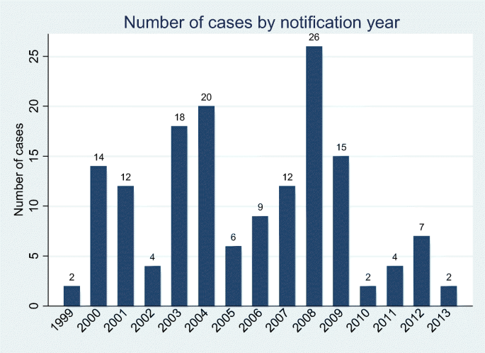
Number of state aid cases by notification year. This figure shows the evolution by year of the number of State aid cases that were notified to the European Commission by the Belgian government. Note that we only include cases that were “active” from 2003 to 2011, which explains the low number of cases notified before and after this period
Article 107 (1) of the Treaty on the Functioning of the European Union expresses this negative presumption on State aid and states that “any aid granted by a Member State or through State resources in any form whatsoever which distorts or threatens to distort competition by favouring certain undertakings or the production of certain goods shall, in so far it affects trade between Member States, be incompatible with the internal market.”
The rules on these exemptions and all other legislation regarding State aid (control) within the European union can be found at http://ec.europa.eu/competition/state_aid/legislation/legislation.html. Member States are required to notify their State aid plans before implementation to the European Commission. However, if the General Block Exemption Regulation or the De Minimis Regulation are applicable, this exempts numerous State aid measures from the notification obligation. Exempted aid is forwarded to the Commission following implementation.
If we assume that the capital used in the production process follows the law of motion kit = (1 − δ)kit − 1 + iit − 1 where δ is the depreciation rate and iit is the investment in capital, then kit is determined entirely by decisions made at time t − 1. Hence, kit is part of the firm’s information set at time t.
We only consider the primary sectors in which the firm is active.
We also examined the different values of the current ratio when conditioning on size, measured by ln(total assets) and by ln(employment). The big differences depend largely on firm size differences between the sectors which confirms that size is an important predictor of financial constraints (see Table 6)
Hadlock and Pierce (2010) point out that the size and the age of the firm are the most consistent predictors of financial constraints. They suggest a financial constraints-index based solely on these (relatively exogenous) firm characteristics.
For more information regarding issues with estimating the outcome of subsidies and state aid, see e.g. Klette et al. (2000). If the government is mainly interested in keeping companies alive (for instance because of employment of their workers), the coefficient of State aid will be downward biased.

References
Ackerberg D, Caves K, Frazer G (2006) Structural identification of production functions. Mimeo
Aghion P, Fally T, Scarpetta S (2007) Credit constraints as a barrier to he entry and post-entry growth of firms. Econ Policy 22(52):731–779
Aghion P, Cai J, Dewatripont M, Du L, Harrison A, Legros P (2015) Industrial Policy and Competition. Am Econ J Macroecon 7(4). https://doi.org/10.1257/max.20120103
Beck T, Demirgüç-Kunt A, Maksimovic V (2005) Financial and legal constraints to growth: does firms size matter? J Financ 60(1):137–177. https://doi.org/10.1111/j.1540-6261.2005.00727.x
Becker B (2015) Public R&D Policies and private R&D investment: a survey of the empirical evidence. J Econ Surv 29(5):917–942. https://doi.org/10.1111/joes.12074
Bernini M, Guillou S, Bellone F (2015) Financial leverage and export quality: Evidence from France. J Bank Financ:280–296. https://doi.org/10.1016/j.jbankfin.2015.06.014
Buts C, Jegers M (2013) The effect of 'State Aid' on market shares: an empirical investigation in an EU member state. J Ind Competition Trade 13(1):88–100
Caballero RJ, Hoshi T, Kashyap AK (2008) Zombie lending and depressed restructuring in Japan. Am Econ Rev 98(5):1943–1977. https://doi.org/10.1257/aer.98.5.1943
Canton E, Grilo I, Monteagudo J, van der Zwan (2013) Perceived credit constraints in the European Union. Small Bus Econ 41(3):701–715. https://doi.org/10.1007/s11187-012-9451-y
Carreira C, Silva F (2010) No deep pockets: some stylized empirical results on firms' financial constraints. J Econ Surv 24(4):731–753. https://doi.org/10.1111/j.1467-6419.2009.00619.x
Cleary S (1999) The relationship between firm investment and financial status. J Financ 54(2):673–692. https://doi.org/10.1111/0022-1082.00121
Coad A, Segarra A, Teruel M (2016) Innovation and firm growth : does firm age play a role? Res Policy 45(2):387–400. https://doi.org/10.1016/j.respol.2015.10.015
Cohen WM, Klepper S (1996) Firm size and the anture of innovation within industries: the case of process and product R&D. Rev Econ Stat 78:232–243. https://doi.org/10.2307/2109925
Czarnitzki D (2006) Research and Development in small and medium-sized enterprises: the role of financial constraints and public funding. Scott J Pol Econ 53(3):335–375. https://doi.org/10.1111/j.1467-9485.2006.00383.x
De Loecker J (2011) Product differentiation, multiproduct firms, and estimating the impact of trade liberalization on productivity. Econometrica 79(5):1407–1451
Fan H, Lai EL-C, Li YA (2015) Credit constraints, quality, and export prices: theory and evidence from China. J Comp Econ 43:390–416. https://doi.org/10.1016/j.jce.2015.02.007
Fix E, Hodges J (1951) Discriminatory analysis, nonparametric discrimination: consistency properties, technical report 4. USAF School of Aviation Medicine, Randolph Field, Texas
Foster L, Haltiwanger J, Syverson C (2008) Reallocation, firm turnover, and efficiency: selection on productivity or profitability. Am Econ Rev 98(1):394–425. https://doi.org/10.1257/aer.98.1.394
Friederiszick HW, Röller L-H, Verouden V (2006) European state aid control: an economic framework. Handbook of antritrust economics:625–669
Grigolon L, Leheyda N, Verboven F (2016) Scrapping schemes in the financial crisis – evidence from Europe. Int J Ind Organ 44:41–59. https://doi.org/10.1016/j.ijindorg.2015.10.004
Gual J, Jódar-Rosel S (2006) Vertical industrial policy in the EU: An empirical analysis of the effectiveness of state aid. "La Caixa" Economic Papers, No.1, https://doi.org/10.1111/j.1360-0443.2006.01518.x
Hadlock CJ, Pierce JR (2010) New evidence on measuring financial constraints: moving beyond the KZ index. Rev Financ Stud 23(5):1909–1940. https://doi.org/10.1093/rfs/hhq009
Hall B (2002) The financing of research and development. Oxf Rev Econ Policy 18(1):35–51. https://doi.org/10.1093/oxrep/18.1.35
Hall BH, Lerner J (2010) The financing of R&D and innovation. Handbook of the Economics of Innovation 1:609–639
Heim S, Hüschelrath K, Schmidt-Dengler P, Strazzeri M (2017) The impact of state aid on the survival and financial viability of aided firms. Eur Econ Rev:193–214
Hurst E, Pugsley B (2011) What do small businesses do? NBER Working Papers, No 17041
Hyytinen A, Toivanen O (2005) Do financial constraints hold back innovation and growth?: evidence on the role of public policy. Res Policy 34(9):1385–1403. https://doi.org/10.1016/j.respol.2005.06.004
Kamien MI, Schwartz NL (1978) Self-financing of an R and D project. Am Econ Rev:252–261
Kleiner T (2005) Reforming state aid policy to best contribute to the Lisbon strategy for growth and jobs. Competition Policy Newsletter, Number 2
Klette TJ, Møen J, Griliches Z (2000) Do subsidies to commercial R&D reduce market failures? Microeconometric evaluation studies. Res Policy 29(4):471–495
Levenson AR, Willard KL (2000) Do firms get the financing they want? Measuring credit rationing experienced by small businesses in the US. Small Bus Econ 14(2):83–94. https://doi.org/10.1023/A:1008196002780
Levinsohn J, Petrin A (2003) Estimating production functions using inputs to control for unobservables. Rev Econ Stud 70(2):317–341. https://doi.org/10.1111/1467-937X.00246
McGowan MA, Andrews D, Millot V (2017) Zombie firms and Productivity Performance in OECD Countries. OECD Economics Department Working Papers, No.132
Modigliani F, Miller MH (1958) The cost of capital, corporation finance and the theory of investment. Am Econ Rev 48(3):261–297
Musso P, Schiavo S (2008) The impact of financial constraints on firm survival and growth. J Evol Econ 18(2):135–149. https://doi.org/10.1007/s00191-007-0087-z
Nitsche R, Heidhues P (2006) Study on methods to analyse the impact of State aid on competition (No. 244). Directorate General Economic and Financial Affairs (DG ECFIN), European Commission
Olley GS, Pakes A (1996) The dynamics of productivity in the telecommunications equipment industry. Econometrica 64(6):1263–1297. https://doi.org/10.2307/2171831
Rajan RG, Zingales L (1998) Which capitalism? Lessons from the east Asian crisis. J Appl Corp Financ 11(3):40–48. https://doi.org/10.1111/j.1745-6622.1998.tb00501.x
Savignac F (2008) Impact of financial constraints on innovation: what can be learned from a direct measure? Econ Innov New Techn 17(6):553–569. https://doi.org/10.1080/10438590701538432
Syverson C (2011) What determines productivity? J Econ Lit 49(2):326–365. https://doi.org/10.1257/jel.49.2.326
Tan Y, Huan Y, Woo WT (2016) Zombie firms and the crowding-out of private Investment in China. Asean Economic Papers 15(3):32–55
Wooldridge JM (2002) Econometric analysis of cross section and panel data. The MIT Press
Wooldrigde JM (2009) On estimating firm-level production functions using proxy variables to control for unobservables. Econ Lett 104(3):112–114. https://doi.org/10.1016/j.econlet.2009.04.026
Acknowledgments
The authors thank Jozef Konings, Dirk Czarnitzki, and Johannes Van Biesebroeck for contributing their insights on earlier versions of the paper as presented during informal seminars at the Department of Economics. The paper benefitted equally from comments by Otto Toivanen, Hans Friederiszick, and Caroline Buts, as well as other participants of the “State Aid Control: Where Law and Economics meet” conference, which was held in Brussels in September 2016. We also thank Louise Birrell for proofreading the article. This work was supported by the KU Leuven [Program Financing of the KU Leuven] & Methusalem [KU Leuven Research Fund Project DOE-C9724-METH/14/01].
Author information
Authors and Affiliations
Corresponding author
Rights and permissions
Open Access This article is distributed under the terms of the Creative Commons Attribution 4.0 International License (http://creativecommons.org/licenses/by/4.0/), which permits unrestricted use, distribution, and reproduction in any medium, provided you give appropriate credit to the original author(s) and the source, provide a link to the Creative Commons license, and indicate if changes were made.
About this article

Cite this article
Sergant, I., Van Cayseele, P. Financial Constraints: State Aid to the Rescue? Empirical Evidence from Belgian Firm-Level Data. J Ind Compet Trade 19, 33–67 (2019). https://doi.org/10.1007/s10842-018-0277-4
Received:
Revised:
Accepted:
Published:
Issue Date:
DOI: https://doi.org/10.1007/s10842-018-0277-4