Cyclic Hypersequent System for Transitive Closure Logic

Abstract

We propose a cut-free cyclic system for transitive closure logic (TCL) based on a form of hypersequents, suitable for automated reasoning via proof search. We show that previously proposed sequent systems are cut-free incomplete for basic validities from Kleene Algebra (KA) and propositional dynamic logic ($\text {PDL}$), over standard translations. On the other hand, our system faithfully simulates known cyclic systems for KA and $\text {PDL}$, thereby inheriting their completeness results. A peculiarity of our system is its richer correctness criterion, exhibiting ‘alternating traces’ and necessitating a more intricate soundness argument than for traditional cyclic proofs.

1 Introduction

Transitive closure logic ($\text {TCL}$) is the extension of first-order logic by an operator computing the transitive closure of definable binary relations. It has been studied by numerous authors, e.g. [15,16,17], and in particular has been proposed as a foundation for the mechanisation and automation of mathematics [18].

Recently, Cohen and Rowe have proposed non-wellfounded and cyclic systems for $\text {TCL}$ [8, 10]. These systems differ from usual ones by allowing proofs to be infinite (finitely branching) trees, rather than finite ones, under some appropriate global correctness condition (the ‘progressing criterion’). One particular feature of the cyclic approach to proof theory is the facilitation of automation, since complexity of inductive invariants is effectively traded off for a richer proof structure. In fact this trade off has recently been made formal, cf. [1, 11], and has led to successful applications to automated reasoning, e.g. [6, 7, 25, 28, 29].

In this work we investigate the capacity of cyclic systems to automate reasoning in $\text {TCL}$ (refer to Fig. 1 for a summary of our contributions). Our starting point is the demonstration of a key shortfall of Cohen and Rowe’s system: its cut-free fragment, here called $\textsf{TC}_G$, is unable to cyclically prove even standard theorems of relational algebra, e.g. $(a\cup b)^* = a^*(ba^*)^*$ and $(aa \cup aba)^+ \le a^+((ba^+)^+ \cup a)$) (Theorem 3.7). An immediate consequence of this is that cyclic proofs of $\textsf{TC}_G$ do not enjoy cut-admissibility (Corollary 3.14). On the other hand, these (in)equations are theorems of Kleene Algebra (KA) [19, 20], a decidable theory which admits automation-via-proof-search thanks to the recent cyclic system of Das and Pous [13].

Fig. 1

The diagram displays results from the literature together with our contributions, marked with . Double arrows represent soundness and completeness results, which for $\text {PDL}^+$ and the class of cyclic sequent proofs $\textsf{L}\textsf{PD}$ is known from [21] (cfr. Sect. 6.1). Hooked arrows represent simulations via translations: $\text {PDL}^+$ can be simulated by $\text {TCL}$, under the standard translation (cfr. Sect. 3.2). $\textsf{TC}_G$ is the class of cyclic sequent proofs for $\text {TCL}$, introduced in [10], that cannot simulate $\textsf{L}\textsf{PD}$ proofs (cfr. Sect. 3.3). Our contribution is the hypersequential and cyclic proof system $\mathsf H\textsf{TC}$, for which we prove soundness (Sect. 5) and completeness via simulation of $\textsf{L}\textsf{PD}$ (Sect. 6). These results can be extended to full $\text {PDL}$ and $\text {TCL}^=$ (with identity), indicated by the right components of each node (in blue)

What is more, $\text {TCL}$ is well-known to interpret Propositional Dynamic Logic ($\text {PDL}$), a modal logic whose modalities are just terms of KA, by a natural extension of the ‘standard translation’ from (multi)modal logic to first-order logic (see, e.g., [2, 3]). Incompleteness of cyclic-$\textsf{TC}_G$ for $\text {PDL}$ over this translation is inherited from its incompleteness for KA. This is in stark contrast to the situation for modal logics without fixed points: the standard translation from K (and, indeed, all logics in the ‘modal cube’) to first-order logic actually lifts to cut-free proofs for a wide range of modal logic systems, cf. [22, 23].

A closer inspection of the systems for KA and $\text {PDL}$ reveals the stumbling block to any simulation: these systems implicitly conduct a form of ‘deep inference’, by essentially reasoning underneath $\exists$ and . Inspired by this observation, we propose a form of hypersequents for predicate logic, with extra structure admitting the deep reasoning required. We present the cut-free system $\mathsf H\textsf{TC}$ and a novel notion of cyclic proof for these hypersequents. In particular, the incorporation of some deep inference at the level of the rules necessitates an ‘alternating’ trace condition corresponding to alternation in automata theory.

Our first main result is the Soundness Theorem (Theorem 5.1): non-wellfounded proofs of $\mathsf H\textsf{TC}$ are sound for standard semantics. The proof is rather more involved than usual soundness arguments in cyclic proof theory, due to the richer structure of hypersequents and the corresponding progress criterion. Our second main result is the Simulation Theorem (Theorem 6.1): $\mathsf H\textsf{TC}$ is complete for $\text {PDL}$ over the standard translation, by simulating a cut-free cyclic system for the latter. This result can be seen as a formal interpretation of cyclic modal proof theory within cyclic predicate proof theory, in the spirit of [22, 23]. To simplify the exposition, we shall mostly focus on equality-free $\text {TCL}$ and ‘identity-free’ $\text {PDL}$ during this paper, though we indeed present an extension to the general case (for $\text {TCL}$ with equality and $\text {PDL}$ with tests) towards the end of this paper in Sect. 7.

The paper is structured as follows. Section 2 introduces $\text {TCL}$, its semantics, and the cyclic sequent calculus for $\text {TCL}$ from Cohen and Rowe [10]. Section 3 introduces $\text {PDL}^+$, the identity-free version of $\text {PDL}$, and the standard translation, and shows that the cyclic system for $\text {TCL}$ by Cohen and Rowe is incomplete for $\text {PDL}^+$. Section 4 presents the cyclic hypersequent calculus for $\text {TCL}$, Sect. 5 shows that it is sound and Sect. 6 proves its completeness over $\text {PDL}^+$ with respect to the standard translation via a cyclic sequent calculus for $\text {PDL}^+$. Finally, Sect. 7 discusses the extension of our calculus to full $\text {TCL}$ and $\text {PDL}$, and Sect. 8 presents further insights and conclusions.

This paper is a full version of the conference paper [12] published at IJCAR ’22. It extends the conference version by providing full definitions, detailed proofs and additional examples.

2 Preliminaries

We shall work with a fixed first-order vocabulary consisting of a countable set $\textsf{Pr}$ of unary predicate symbols, written p, q,  etc., and of a countable set $\textsf{Rel}$ of binary relation symbols, written a, b,  etc. We build formulas from this language differently in the modal and predicate settings, but all our formulas may be formally evaluated within structures:

Definition 2.1

(Structures) A structure $\mathcal M$ consists of a set D, called the domain of $\mathcal M$, which we sometimes denote by $\mid \!\!\mathcal M\!\!\mid$; a subset $p^{\mathcal M} \subseteq D$ for each $p \in \textsf{Pr}$; and a subset $a^{\mathcal M} \subseteq D\times D$ for each $a \in \textsf{Rel}$.

As above, we shall generally distinguish the words ‘predicate’ (unary) and ‘relation’ (binary). We could include further relational symbols too, of higher arity, but choose not to in order to calibrate the semantics of both our modal and predicate settings.

2.1 Transitive Closure Logic

In addition to the language introduced at the beginning of this section, in the predicate setting we further make use of a countable set of function symbols, written $f^i,g^j,$ etc., where the superscripts $i,j \in \mathbb N$ indicate the arity of the function symbol and may be omitted when it is not ambiguous. Nullary function symbols (aka constant symbols), are written ${c}, {d}$ etc. We shall also make use of variables, written x, y,  etc., typically bound by quantifiers. Terms, written s, t,  etc., are generated as usual from variables and function symbols by function application. A term is closed if it has no variables.

We consider the usual syntax for first-order logic formulas over our language, with an additional operator for transitive closure (and its dual). Formally $\text {TCL}$ formulas, written A, B,  etc., are generated as follows:

When variables x, y are clear from context, we may write $TC ({A(x,y)})(s,t)$ or $TC ({A})(s,t)$ instead of $TC ({\lambda x,y.A})(s,t)$, as an abuse of notation, and similarly for $\overline{ TC }$. Without loss of generality, we assume that the same variable cannot occur free and bound within the scope of the quantifiers, $TC$- and $\overline{ TC }$-formulas. We write A[t/x] for the formula obtained from A by replacing every free occurrence of the variable x by the term t. The choice of allowing negation only on atomic proposition, and not including implication as a primitive operator in the language, is motivated by the fact that we will opt for a one-sided definition of sequents.

Remark 2.2

(Equality) Note that we do not include term equality among our atomic formulas at this stage. Later we shall indeed consider such extensions, for which the syntax and semantics are as usual for predicate logic.

Definition 2.3

(Duality) For a formula A we define its complement, $\bar{A}$, by:

We shall employ standard logical abbreviations, e.g. $A\rightarrow B$ for . We may evaluate formulas with respect to a structure, but we need additional data for interpreting function symbols:

Definition 2.4

(Interpreting function symbols) Let $\mathcal M$ be a structure with domain D. An interpretation is a map $\rho$ that assigns to each function symbol $f^n$ a function $D^n \rightarrow D$. We may extend any interpretation $\rho$ to an action on (closed) terms by setting recursively $\rho (f(t_1, \dots , t_n)) :=\rho (f)(\rho (t_1), \dots , \rho (t_n))$.

We only consider standard semantics in this work: $TC$ (and $\overline{ TC }$) is always interpreted as the real transitive closure (and its dual) in a structure, rather than being axiomatised by some induction (and coinduction) principle.

In order to facilitate the formal definition of satisfaction, namely for the quantifier and reflexive transitive closure cases, we shall adopt a standard convention of assuming among our constant symbols arbitrary parameters from the model $\mathcal M$. Formally this means that we construe each $v\in D$ as a constant symbol for which we shall always set $\rho (v) = v$.

Definition 2.5

(Semantics) Given a structure $\mathcal M$ with domain D and an interpretation $\rho$, the judgement $\mathcal M,\rho \models A$ is defined as follows:

• $\mathcal M, \rho \models p(t)$ if $\rho (t) \in p^{\mathcal M}$.

• $\mathcal M, \rho \models \bar{p}(t)$ if $\rho (t) \notin p^{\mathcal M}$.

• $\mathcal M, \rho \models a(s,t)$ if $(\rho (s), \rho (t)) \in a^{\mathcal M}$.

• $\mathcal M, \rho \models \bar{a}(s,t)$ if $(\rho (s),\rho (t)) \notin a^{\mathcal M}$.

• if $\mathcal M,\rho \models A$ and $\mathcal M,\rho \models B$.

• if $\mathcal M,\rho \models A$ or $\mathcal M,\rho \models B$.

• $\mathcal M,\rho \models \forall x A$ if, for every $v \in D$, we have $\mathcal M,\rho \models A[v/x]$.

• $\mathcal M,\rho \models \exists x A$ if, for some $v \in D$, we have $\mathcal M,\rho \models A[v/x]$.

• $\mathcal M,\rho \models TC ({A})(s,t)$ if there are $v_0, \dots , v_{n+1} \in D$ with $\rho (s) = v_0$, $\rho (t)=v_{n+1}$, such that for every $i\le n$ we have $\mathcal M,\rho \models A(v_i,v_{i+1})$.

• $\mathcal M, \rho \models \overline{ TC }({A})(s,t)$ if for all $v_0, \dots , v_{n+1} \in D$ with $\rho (s)=v_0$ and $\rho (t)=v_{n+1}$, there is some $i\le n$ such that $\mathcal M,\rho \models A(v_i,v_{i+1})$.

If $\mathcal M,\rho \models A$ for all $\mathcal M$ and $\rho$, we simply write $\models A$.

As expected, we have $\mathcal M, \rho \not \models TC ({A})(s,t)$ just if $\mathcal M,\rho \models \overline{ TC }({\bar{A}})(s,t)$, and so the two operators are semantically dual. The following statement, that easily follows from the semantics clauses defined above, demonstrates that $TC$ and $\overline{ TC }$ duly correspond to least and greatest fixed points.

Fact 2.6

($TC$ and $\overline{ TC }$ as least and greatest fixed points) The following hold, for arbitrary $\mathcal M$, $\rho$ and x:

We have included both $TC$ and $\overline{ TC }$ as primitive so that we can reduce negation to atomic formulas, allowing a one-sided formulation of proofs. Let us point out that our $\overline{ TC }$ operator is not the same as Cohen and Rowe’s transitive ‘co-closure’ operator $TC ^{ op }$ in [9]. As they already note there, $TC ^{ op }$ cannot be defined in terms of $TC$ (using negations), whereas $\overline{ TC }$ is the formal De Morgan dual of $TC$ and, in the presence of negation, are indeed interdefinable, cf. Definition 2.3.

2.2 Cohen–Rowe Cyclic System for $\text {TCL}$

Cohen and Rowe proposed in [8, 10] a non-wellfounded sequent system for $\text {TCL}$ (with equality) extending a standard sequent calculus $\textsf{L}\mathsf K^=$ for first-order logic with equality and substitution by rules for $TC$ inspired by its characterisation as a least fixed point, cf. Fact 2.6. A non-wellfounded proof system allows for infinitely long branches, provided that they satisfy a logic-specific progress condition. Here we present a one-sided variation of (the cut-free fragment of) their system, both with and without equality.

Fig. 2

Above: Sequent calculus $\textsf{TC}_G$. The first two lines of the Figure contain the rules of the Tait-style sequent system for first-order predicate logic, without equality. The constant symbol c in the $\forall$-rule and the $\overline{ TC }$-rule is called an eigenvariable. Below: The standard rules for equality. When added to $\textsf{TC}_G$, they give the sequent calculus $\textsf{TC}^=_G$. Colours define traces (see Remark 2.9)

Definition 2.7

(System) A sequent, written $\Gamma ,\Delta$ etc., is a set of formulas. The systems $\textsf{TC}_G$ and $\textsf{TC}^=_G$ are given in Fig. 2: $\textsf{TC}^=_G$ consists of all the rules displayed, while $\textsf{TC}_G$ does not include the $=$ or $\ne$ rules. $\textsf{TC}_G^{(=)}$-preproofs are possibly infinite trees of sequents generated by the rules of $\textsf{TC}_G^{(=)}$ (colours may be ignored for now). A preproof is regular if it has only finitely many distinct sub-preproofs.

In Fig. 2$\sigma$ is a map (“substitution”) from constants to terms and other function symbols to function symbols of the same arity, extended to terms, formulas and sequents in the natural way. The substitution rule is redundant for usual provability, but facilitates the definition of ‘regularity’ in predicate cyclic proof theory.

The notions of non-wellfounded and cyclic proofs for $\textsf{TC}_G^{(=)}$ are formulated similarly to those for first-order logic with (ordinary) inductive definitions [5]:

Definition 2.8

(Traces and proofs) Given a $\textsf{TC}_G^{(=)}$ preproof $\mathcal {D}$ and a branch $\mathcal B= (\mathsf r_i)_{i \in \omega }$ (where each $\mathsf r_i$ is an inference step), a trace is a sequence of formulas of the form $(\overline{ TC }({A})(s_i,t_i))_{i\ge k}$ such that for all $i\ge k$ either:

• 1. $\mathsf r_i$ is not a substitution step and $(s_{i+1}, t_{i+1}) = (s_i,t_i)$; or,

• 2. $\mathsf r_i$ is a $\overline{ TC }$ step with principal formula $\overline{ TC }({A})(s_i,t_i)$ and $(s_{i+1}, t_{i+1}) = ({c},t_i)$, where ${c}$ is the eigenvariable of $\mathsf r_i$; or,

• 3. $\mathsf r_i$ is a substitution step with respect to $\sigma$ and $(\sigma (s_{i+1}), \sigma (t_{i+1}) ) = (s_i,t_i)$.

We say that the trace is progressing if the case 2 above happens infinitely often along it. A $\textsf{TC}_G^{(=)}$-preproof $\mathcal {D}$ is a proof if each of its infinite branches has a progressing trace. If $\mathcal {D}$ is regular we call it a cyclic proof. We write $\textsf{TC}_G^{(=)} \vdash _ cyc A$ if there is a cyclic proof in $\textsf{TC}_G^{(=)}$ of A.

Remark 2.9

(Traces via colours) Fig. 2 codes the notion of trace by means of colours: along any infinite branch a trace is a monochromatic sequence of formulas (with inference steps as displayed in Fig. 2); if the trace hits a formula in the context ${\Gamma }$ in the conclusion of an inference step, it must hit the same formula in the premiss it follows.

Proposition 2.10

(Soundness, [8, 10]) If $\textsf{TC}_G^{(=)} \vdash _ cyc A$ then $\models A$.

In fact (the equality-free version of) this result is subsumed by our main soundness result for $\mathsf H\textsf{TC}$ (Theorem 5.1) and its simulation of $\textsf{TC}_G$ (Theorem 4.11). A partial converse of Proposition 2.10 is available in the presence of a cut rule:

Namely, cyclic $\textsf{TC}_G^{(=)}$ proofs are ‘Henkin complete’, i.e. complete for all models of a particular axiomatisation of $\text {TCL}$ (with or withour equality, resp.) based on (co)induction principles [8, 10]. However, the counterexample we present in the next section implies that cut is not eliminable (Corollary 3.14).

2.3 Differences to [8, 10]

Our formulation of $\textsf{TC}_G^{(=)}$ differs slightly from the original presentation in [8, 10], but in no essential way. Nonetheless, let us survey these differences now.

2.3.1 One-Sided vs. Two-Sided

Cohen and Rowe employ a two-sided calculus as opposed to our one-sided one, but the difference is purely cosmetic. Sequents in their calculus are written $A_1, \dots , A_m \Rightarrow B_1, \dots , B_n$, which may be duly interpreted in our calculus as $\bar{A}_1, \dots , \bar{A}_m, B_1, \dots , B_n$. Indeed we may write sequents in this two-sided notation at times in order to facilitate the reading of a sequent and to distinguish left and right formulas. For this reason, Cohen and Rowe do not include a $\overline{ TC }$ operator in their calculus, but are able to recover it thanks to a formal negation symbol, cf. Definition 2.3.

2.3.2 TC vs. RTC

Cohen and Rowe’s system is originally called $\mathsf R \textsf{TC}_G$, rather using a ‘reflexive’ version $RTC$ of the $TC$ operator. As they mention, this makes no difference in the presence of equality. Semantically we have , but this encoding does not lift to proofs, i.e. the $RTC$ rules of [8] are not locally derived in $\textsf{TC}^=_G$ modulo this encoding. However, the encoding suffices for this purpose.

2.3.3 Alternative Rules and Fixed Point Characterisations

Cohen and Rowe use a slightly different fixed point formula to induce rules for $RTC$ and $\overline{ RTC }$ (i.e. $RTC$ on the left) based on the fixed point characterisation,

(1)

decomposing paths ‘from the right’ rather than the left. These alternative rules induce analogous notions of trace and progress for preproofs such that progressing preproofs enjoy a similar soundness theorem, cf. Proposition 2.10. The reason we employ a slight variation of Cohen and Rowe’s system is to remain consistent with how the rules of $\textsf{L}\textsf{PD}^+$ (or $\textsf{L}\textsf{PD}$) and $\mathsf H\textsf{TC}$ (or $\mathsf H\textsf{TC}^=$) are devised later. To the extent that we prove things about $\textsf{TC}_G^{(=)}$, namely its (cut-free) regular incompleteness in Theorem 3.7, the particular choice of rules turns out to be unimportant. The counterexample we present there is robust: it applies to systems with any (and indeed all) of the above rules.

3 Interlude: Motivation from PDL

Given the $\text {TCL}$ sequent system proposed by Cohen and Rowe, why do we propose a hypersequential system? Our main argument is that proof search in $\textsf{TC}_G^{(=)}$ is rather weak, to the extent that cut-free cyclic proofs are unable to simulate a basic (cut-free) system for modal logic $\text {PDL}$ (regardless of proof search strategy). At least one motivation here is to ‘lift’ the standard translation from cut-free cyclic proofs for $\text {PDL}$ to cut-free cyclic proofs in an adequate system for $\text {TCL}$ (with equality).

3.1 Identity-Free PDL

Identity-free propositional dynamic logic ($\text {PDL}^+$) is a version of the modal logic $\text {PDL}$ without tests or identity, thereby admitting an ‘equality-free’ standard translation into predicate logic. Formally, $\text {PDL}^+$ formulas, written A, B,  etc., and programs, written $\alpha , \beta ,$ etc., are generated by the following grammars:

Remark 3.1

(Formula metavariables) We are using the same metavariables A, B,  etc. to vary over both $\text {PDL}^+$ and $\text {TCL}$ formulas. This should never cause confusion due to the context in which they appear. Moreover, this coincidence is suggestive, since many notions we consider, such as duality and satisfaction, are defined in a way that is compatible with both notions of formula.

Definition 3.2

(Duality) For a formula A we define its complement, $\bar{A}$, by:

We evaluate $\text {PDL}^+$ formulas using the traditional relational semantics of modal logic, by associating each program with a binary relation in a structure. Again, we only consider ‘standard’ semantics:

Definition 3.3

(Semantics) Fix a structure $\mathcal M$ with domain D. For elements $v \in D$ and programs $\alpha$ we define $\alpha ^{\mathcal M}\subseteq D\times D$ by:

• ($a^{\mathcal M}$ is already given in the specification of $\mathcal M$, cf. Definition 2.1).

• $(\alpha \beta )^{\mathcal M}:= \{ (u,v): \text {there is } w\in D \text { s.t.\ } (u,w) \in \alpha ^{\mathcal M}\text { and } (w,v) \in \beta ^{\mathcal M}\}$.

• $(\alpha \cup \beta )^{\mathcal M}:= \{ (u,v): (u,v) \in \alpha ^{\mathcal M}\text { or } (u,v) \in \beta ^{\mathcal M}\}$.

• $(\alpha ^+)^{\mathcal M}:= \{ (u,v): \text {there are } w_0, \dots , w_{n+1} \in D \text { s.t.\ } u = w_0, v = w_{n+1} \text { and } \text {for }$ $\text {every } i\le n \text { we have } (w_i,w_{i+1}) \in \alpha ^{\mathcal M}\}$.

For elements $v\in D$ and formulas A we also define the judgement $\mathcal M, v \models A$ by:

• $\mathcal M,v \models p$ if $v \in p^{\mathcal M}$.

• $\mathcal M,v \models \overline{p}$ if $v \notin p^{\mathcal M}$.

• if $\mathcal M, v \models A$ and $\mathcal M, v \models B$.

• if $\mathcal M, v \models A$ or $\mathcal M, v \models B$.

• $\mathcal M, v \models [\alpha ] A$ if for every $(v,w) \in \alpha ^{\mathcal M}$ we have $\mathcal M, w \models A$.

• $\mathcal M, v \models \langle \alpha \rangle A$ if there exists $(v,w) \in \alpha ^{\mathcal M}$ with $\mathcal M,w \models A$.

If $\mathcal M,v \models A$ for all $\mathcal M$ and $v\in D$, then we write $\models A$.

Note that we are overloading the satisfaction symbol $\models$ here, for both $\text {PDL}^+$ and $\text {TCL}$. This should never cause confusion, in particular since the two notions of satisfaction are ‘compatible’, given that we employ the same underlying language and structures. In fact such overloading is convenient for relating the two logics, as we shall now see.

3.2 The Standard Translation

The so-called “standard translation” of modal logic into predicate logic is induced by reading the semantics of modal logic as first-order formulas. We now give a natural extension of this that interprets $\text {PDL}^+$ into $\text {TCL}$. At the logical level our translation coincides with the usual one for basic modal logic; our translation of programs, as expected, requires the $TC$ operator to interpret the $+$ of $\text {PDL}^+$.

Definition 3.4

For a $\text {PDL}^+$ formula A and program $\alpha$, we define the standard translations $\textsf{ST}(A)({x})$ and $\textsf{ST}(\alpha )({x,y})$ as $\text {TCL}$-formulas with free variables x and x, y, resp., inductively as follows,

where we have written simply $TC (\textsf{ST}(\alpha ))$ instead of $TC (\lambda x,y.\textsf{ST}(\alpha )({x,y}))$.

Example 3.5

By means of example, consider the following formulas:

It is routine to show that $\overline{\textsf{ST}(A)({x})} = \textsf{ST}(\bar{A})({x})$, by structural induction on A, justifying our overloading of the notation $\bar{A}$, in both $\text {TCL}$ and $\text {PDL}^+$. Yet another advantage of using the same underlying language for both the modal and predicate settings is that we can state the following (expected) result without the need for encodings, following by a routine structural induction (see, e.g., [3]):

Theorem 3.6

For $\text {PDL}^+$ formulas A, we have $\mathcal M,v \models A$ iff $\mathcal M \models \textsf{ST}(A)({v})$.

3.3 Cohen–Rowe System is Not Complete for $\text {PDL}^+$

$\text {PDL}^+$ admits a standard cut-free cyclic proof system $\textsf{L}\textsf{PD}^+$ (see Sect. 6.1) which is both sound and complete (cf. Theorem 6.4). However, a shortfall of $\textsf{TC}_G$ is that it is unable to cut-free simulate $\textsf{L}\textsf{PD}^+$. In fact, we can say something stronger:

Theorem 3.7

(Incompleteness) There exist a $\text {PDL}^+$ formula A such that $\models A$ but $\textsf{TC}_G\not \vdash _ cyc \textsf{ST}(A)({x})$ (in the absence of cut).

This means not only that $\textsf{TC}_G$ is unable to locally cut-free simulate the rules of $\textsf{L}\textsf{PD}^+$, but also that there are some validities for which there are no cut-free cyclic proofs at all in $\textsf{TC}_G$. One example of such a formula is:

$$\begin{aligned} \langle (aa\cup aba)^+\rangle p \rightarrow \langle a^+((ba^+)^+ \cup a)\rangle p. \end{aligned}$$

(2)

This formula is derived from the well-known $\text {PDL}$ validity $\langle (a\cup b)^*\rangle p \rightarrow \langle a^*(ba^*)^*\rangle p$ by identity-elimination. This in turn is essentially a theorem of relational algebra, namely $(a\cup b)^* \le a^*(ba^*)^*$, which is often used to eliminate $\cup$ in (sums of) regular expressions. The same equation was (one of those) used by Das and Pous in [13] to show that the sequent system $\textsf{LKA}$ for Kleene Algebra is cut-free cyclic incomplete.

In the remainder of this subsection, we shall give a proof of Theorem 3.7. The argument is much more involved than the one from [13], due to the fact we are working in predicate logic, but the underlying basic idea is similar. At a very high level, the right-hand side of (2) (viewed as a relational inequality) is translated to an existential formula that, along some branch (namely the one that always chooses aa when decomposing the LHS of (2)) can never be instantiated while remaining valid. This branch witnesses the non-regularity of any proof.

3.3.1 Some Closure Properties for Cyclic Proofs

Demonstrating that certain formulas do not have (cut-free) cyclic proofs is a delicate task, made more so by the lack of a suitable model-theoretic account (indeed, cf. Corollary 3.14). In order to do so formally, we first develop some closure properties of cut-free cyclic provability.

Proposition 3.8

(Inversions) We have the following:

• 1. If then $\textsf{TC}_G\vdash _ cyc \Gamma , A,B$.

• 2. If then $\textsf{TC}_G\vdash _ cyc \Gamma , A$ and $\textsf{TC}_G\vdash _ cyc \Gamma , B$.

• 3. If $\textsf{TC}_G\vdash _ cyc \Gamma , \forall x A(x)$ then $\textsf{TC}_G\vdash _ cyc \Gamma , A({c})$, as long as ${c}$ is fresh.

Proof Sketch

All three statements are proved similarly.

For item 1, replace every direct ancestor of with A, B. The only critical steps are when is principal, in which case we delete the step, or is weakened, in which case we apply two weakenings, one on A and one on B. If the starting proof had only finitely many distinct subproofs (up to substitution), say n, then the one obtained by this procedure has at most 2n distinct subproofs (up to substitution), since we simulate a weakening on by two weakenings.

For item 2, replace every direct ancestor of with A or B, respectively. The only critical steps are when is principal, in which case we delete the step and take the left or right subproof, respectively, or is weakened, in which case we simply apply a weakening on A or B, respectively. The proof we obtain has at most the same number of distinct subproofs (up to substitution) as the original one.

For item 3, replace every direct ancestor of $\forall x A(x)$ with $A({c})$. The only critical steps are when $\forall x A(x)$ is principal, in which case we delete the step and rename the eigenvariable in the remaining subproof everywhere with ${c}$, or is weakened, in which case we simply apply a weakening on $A({c})$. The proof we obtain has at most the same number of distinct subproofs (up to substitution) as the original one.

Proposition 3.9

(Predicate admissibility) Suppose $\textsf{TC}_G\vdash _ cyc \Gamma , p(t)$ or $\textsf{TC}_G\vdash _ cyc \Gamma , \bar{p}(t)$, where $\bar{p}$ or p (respectively) does not occur in $\Gamma$. Then it holds that $\textsf{TC}_G\vdash _ cyc \Gamma$.

Proof sketch

Delete every ancestor of p(t) or $\bar{p}(t)$, respectively. The only critical case is when one of the formulas is weakened, in which case we omit the step. Note that there cannot be any identity on p, due to the assumption on $\Gamma$, and by the subformula property.

3.3.2 Reducing to a Relational Tautology

Here, and for the remainder of this subsection, we shall simply construe $\text {PDL}^+$ programs $\alpha$ and formulas A as $\text {TCL}$ formulas with two free variables and one free variable, respectively, by identifying them with their standard translations $\textsf{ST}(\alpha )({x,y})$ and $\textsf{ST}(A)({x})$, respectively. This modest abuse of notation will help suppress much of the notation in what follows.

Lemma 3.10

If $\textsf{TC}_G\vdash _ cyc ({\langle (aa \cup aba)^+\rangle p \rightarrow \langle a^+((ba^+)^+\cup a)\rangle p})(c)$ then also $\textsf{TC}_G\vdash _ cyc {(aa \cup aba)^+}(c,d) \rightarrow ({a^+((ba^+)^+\cup a)})(c,d)$.

Proof sketch

Suppose $\textsf{TC}_G\vdash _ cyc ({\langle (aa \cup aba)^+\rangle p \rightarrow \langle a^+((ba^+)^+\cup a)\rangle p})(c)$ so, by unwinding the definition of $\textsf{ST}$ and since duality commutes with the standard translation, cf. Sect. 3.2, we have that . By -inversion (Proposition 3.8.1) we have:

$$\begin{aligned} \textsf{TC}_G\vdash _ cyc ({[(aa \cup aba)^+]\bar{p}})(c), ({\langle a^+((ba^+)^+\cup a)\rangle p})(c). \end{aligned}$$

Again unwinding the definition of $\textsf{ST}$, and by the definition of duality, we thus have:

Now, by $\forall$-inversion and -inversion, Prop. 3.8, we have:

Without loss of generality we may instantiate the $\exists y$ by d and so by -inversion, Prop. 3.8.2, we have:

$$\begin{aligned} \textsf{TC}_G\vdash _ cyc \overline{(aa \cup aba)^+}(c,d), \bar{p}(d), a^+((ba^+)^+ \cup a) (c,d). \end{aligned}$$

Since there is no occurrence of p above, by Prop. 3.9 we conclude

$$\begin{aligned} \textsf{TC}_G\vdash _ cyc \overline{(aa \cup aba)^+}(c,d), a^+((ba^+)^+ \cup a) (c,d), \end{aligned}$$

as required.

3.3.3 Irregularity via an Adversarial Model

In the previous subsubsection we reduced the incompleteness of cut-free cyclic sequent proofs for $\text {TCL}$ over the image of the standard translation on $\text {PDL}^+$ to the non-regular cut-free provability of a particular relational validity. Unwinding this a little, the sequent that we shall show has no (cut-free) cyclic proof in $\textsf{TC}_G$ can be written in ‘two-sided notation’ (cf. Sect. 2.3) as follows:

(3)

This two-sided presentation is simply a notational variant that allows us to more easily reason about the proof search space (e.g. referring to ‘LHS’ and ‘RHS’). Formally:

Convention 3.11

(Two-sided notation) We may write $\Gamma \Rightarrow \Delta$ as shorthand for the sequent $\bar{\Gamma },\Delta$, where $\bar{\Gamma }= \{ \bar{A}: A \in \Gamma \}$. References to the ‘left-hand side (LHS)’ and ‘right-hand side (RHS)’ have the obvious meaning, always with respect to the delimiter $\Rightarrow$.

To facilitate our argument, we shall only distinguish sequents ‘modulo substitution’ rather than allowing explicit substitution steps when reasoning about (ir)regularity of a proof.

We shall design a family of ‘adversarial’ models, and instantiate proof search to just these models. In this way, we shall show that any non-wellfounded $\textsf{TC}_G$ proof of the sequent (3) must have arbitrarily long branches without a repetition (up to substitution). Since $\textsf{TC}_G$ is finitely branching, by König’s Lemma this means that any non-wellfounded $\textsf{TC}_G$ proof of (3) has an infinite branch with no repetitions (up to substitution), as required.

Fig. 3

The adversarial model from Definition 3.12. Solid arrows represent $a^{\mathcal A_{n}}$-relations, dashed arrows $b^{\mathcal A_{n}}$-relations

Definition 3.12

(An adversarial model) For $n\in \mathbb N$, define the structure $\mathcal A_{n}$ by:

• The domain of $\mathcal A_{n}$ is $\{u_0,u_0', \dots , u_{n-1}, u_{n-1}',u_n, v \}$.

• $a^{\mathcal A_{n}} = \{(u_i, u_{i}'),(u_{i}',u_{i+1}) \}_{i<n}$.

• $b^{\mathcal A_{n}} = \{(u_n,v) \}$.

Note that, since the sequent (3) that we are considering is purely relational, it does not matter what sets $\mathcal A_{n}$ assigns to the predicate symbols, so we refrain from specifying such data.

Lemma 3.13

Let $n\in \mathbb N$. Any $\textsf{TC}_G$ proof $\mathcal {D}$ of (3) has a branch with no repetitions (up to substitutions) among its first n sequents.

Proof

Set $c_0=c$. Consider some (possibly finite, but maximal) branch $\mathcal B= (\mathsf r_i)_{i\le \nu }$ (with $\nu \le \omega$) of $\mathcal {D}$ satisfying:

• whenever $TC$ on the LHS is principal (formally speaking, for a $\overline{ TC }$ step), the right premiss is followed; and,

• whenever is principal for any s and t on the LHS (formally speaking, for a step) the left premiss (corresponding to (aa)(s, t)) is followed.

Let $k \le n$ be maximal such that, for each $i\le k$, $\mathsf r_i$ has principal formula on the LHS. Now:

• 1. For $i\le k$, each $\mathsf r_i$ has conclusion with LHS of the form:

  

  (4)

  for some $l\le i$ and distinct $c_0, \dots , c_{l}$ and where each $\Gamma _j(c_{j-1},c_j)$ has the form $a(c_{j-1}, c_{j-1}'),a(c_{j-1}',c_j)$ or or $(aa)(c_{j-1},c_{j})$ or . To see this, proceed by induction on $i\le k$:

  • The base case is immediate, by setting $l=0$.

  • For the inductive step, note that the principal formula of $\mathsf r_i$ must be on the LHS, since $i\le k$. Thus by the inductive hypothesis the principal formula of $\mathsf r_i$ must have the form:

    • , in which case the premiss of $\mathsf r_i$ (which is a step) replaces it by $a(c_{j-1}, c_{j-1}'),a(c_{j-1}',c_j)$; or,

    • $(aa)(c_{j-1},c_j)$, in which case the premiss of $\mathsf r_i$ (which is a $\forall$ step) replaces it by , for $c_{j-1}'$ a fresh symbol; or,

    • , in which case, by definition of $\mathcal B$, the $\mathcal B$-premiss of $\mathsf r_i$ (which is a left- step) replaces this formula by some $a(c_{j-1},c_j)$; or,

    • for some $l\le i$, in which case, by definition of $\mathcal B$, the $\mathcal B$-premiss of $\mathsf r_i$ (which is a left-$TC$ step) replaces it by the cedent .

• 2. Moreover, for $i<i'\le k$, the conclusion of $\mathsf r_i$ and $\mathsf r_{i'}$ are not equal (up to substitution). To see this, note that any rule principal on an LHS of form (4) either decreases the size of some $\Gamma _j(c_{j-1},c_j)$ (when it is a or step) or increases the number of eigenvariables in the sequent (when it is a left $TC$ step), in particular the index l of .

• 3. Since proofs must be sound for all models (by soundness), we shall work in $\mathcal A_{n}$ with respect to an interpretation $\rho _n$ satisfying $c_i \mapsto u_i$ for $i\le n$ and $c_i'\mapsto u_i'$ for $i<n$ and $d \mapsto v$. It follows by inspection of (4) that, for $i\le k$, each formula on the LHS of the conclusion of $\mathsf r_i$ is true in $(\mathcal A_{n}, \rho _n)$.

• 4. Along $\mathcal B$, the RHS cannot be principal unless $l\ge n$ in (4), so in particular $k\ge n$. To see this:

  • Recall that the interpretation $\rho _n$ assigns to $c_0,c_0', \dots , c_{n-1}',c_n$ the worlds $u_0, u_0', \dots , u_{n-1}',u_n$ respectively.

  • If the existential formula on the RHS is instantiated by some $c_i$ or $c_i'$ with $i<n$ then the resulting sequent is false in $(\mathcal A_{n},\rho _n)$ (recall that, by Item 3, every formula on the LHS is true, so we require the RHS to be true too). To see this, note that the RHS in particular would imply $(ba^+)^+(c_i,d)$ or $a(c_i,d)$ or $(ba^+)^+(c_i',d)$ or $a(c_i',d)$. However when $i<n$ none of these formulas are true with respect to $(\mathcal A_{n},\rho _n)$.

  • If the existential formula on the RHS is instantiated by d then the resulting sequent is again false, by the same analysis as above.

By Item 4, we have that $k\ge n$ and so, since we assumed $k\le n$ at the start, indeed $k=n$. Thus, by Item 1 and Item 2, there are no repeated sequents (up to substitution) in $(\mathsf r_i)_{i\le n}$, as required.

3.3.4 Putting It All Together

We are now ready to give the proof of the main result of this section.

Proof of Theorem 3.7, Sketch

Since the choice of n in Lemma 3.13 was arbitrary, any $\textsf{TC}_G$ proof $\mathcal {D}$ of (3) must have branches with arbitrarily long initial segments without any repetition (up to substitution). Since the system is finitely branching, by König’s Lemma we have that there is an infinite branch through $\mathcal {D}$ without any repetition (up to substitution), and thus $\mathcal {D}$ is not regular. Thus $\textsf{TC}_G\not \vdash _ cyc$ (3). Finally, by contraposition of Lemma 3.10, we have, as required:

$$\begin{aligned} \textsf{TC}_G\not \vdash _ cyc ({\langle (aa \cup aba)^+\rangle p \rightarrow \langle a^+((ba^+)^+\cup a)\rangle p})(c). \end{aligned}$$

An immediate consequence of Theorem 3.7 and Henkin-completeness of $\textsf{TC}_G$ with cut [8, 10] is:

Corollary 3.14

The class of cyclic proofs of $\textsf{TC}_G$ does not enjoy cut-admissibility.

4 Hypersequent Calculus for $\text {TCL}$

In light of the preceding subsection, let us take a moment to examine how a ‘local’ simulation of $\textsf{L}\textsf{PD}^+$ by $\textsf{TC}_G$ fails, in order to motivate the main system that we shall present. The program rules, in particular the $\langle \, \rangle$-rules, require a form of deep inference to be correctly simulated, over the standard translation. For instance, let us consider the action of the standard translation on two rules we shall see later in $\textsf{L}\textsf{PD}^+$ (cf. Sect. 6.1):

The first case above suggests that any system to which the standard translation lifts must be able to reason underneath $\exists$ and , so that the inference indicated in blue is ‘accessible’ to the prover. The second case above suggests that the existential-conjunctive meta-structure necessitated by the first case should admit basic equivalences, in particular certain prenexing. This section is devoted to the incorporation of these ideas (and necessities) into a bona fide proof system.

4.1 Annotated Hypersequents

An annotated cedent, or simply cedent, written $S,S'$ etc., is an expression $\{ \Gamma \}^{{\textbf {x}}}$, where $\Gamma$ is a set of formulas and the annotation ${\textbf {x}}$ is a set of variables. We sometimes construe annotations as lists rather than sets when it is convenient, e.g. when taking them as inputs to a function. Each cedent may be intuitively read as a $\text {TCL}$ formula, under the following interpretation:

$$\begin{aligned} fm (\{ \Gamma \}^{x_1, \dots , x_n}) \ :=\ \exists x_1 \dots \exists x_n \bigwedge \Gamma . \end{aligned}$$

When ${\textbf {x}}= \varnothing$ then there are no existential quantifiers above, and when $\Gamma = \varnothing$ we simply identify $\bigwedge \Gamma$ with $\top$. We also sometimes write simply A for the annotated cedent $\{ A\}^{\varnothing }$.

A (annotated) hypersequent, written ${\varvec{S}},{\varvec{S}}'$ etc., is a set of annotated cedents. Each hypersequent may be intuitively read as the disjunction of its cedents. Namely we set: With a slight abuse of notation, we sometimes identify ${\varvec{S}}$ and $fm ({\varvec{S}})$.

4.2 Non-wellfounded Hypersequent Proofs

We now present our hypersequential system for $\text {TCL}$ and its corresponding notion of ‘non-wellfounded proof’.

Definition 4.1

(System) The rules of $\mathsf H\textsf{TC}$ are given in Fig. 4 (the colours may be ignored for now). A $\mathsf H\textsf{TC}$ preproof is a possibly infinite tree of sequents generated by the rules of $\mathsf H\textsf{TC}$. A preproof is regular if it has only finitely many distinct subproofs.

Fig. 4

Hypersequent calculus $\mathsf H\textsf{TC}$, where $\sigma$ is a substitution map from constants to terms and a renaming of other function symbols and variables, extended to terms, formulas, cedents and hypersequents in the natural way. For $\Gamma$ set of formulas, $\textsf{fv}(\Gamma )$ denotes the set of free variables occurring in formulas in $\Gamma$. Colours define ancestry (see Remark 4.4)

The substitution rule $\sigma$ is needed to guarantee regularity of non-wellfounded branches. While we have included an explicit substitution rule we shall, as in earlier sections, often work ‘modulo substitution’ when writing down cyclic preproofs. Propositional rules, as well as $\textsf{init}$, are standard, recalling the formula interpretation of hypersequents defined in the previous section. The $\cup$ rule is the only branching rule of the system, while rule $\textsf{id}$ allows us to eliminate (bottom-up) a closed formula A from one of the cedents (thus from a conjunction, wrt the formula interpretation) provided that the dual of A occurs in a singleton cedent with empty annotation. The usual sequent rule for the existential quantifier is factored into two $\mathsf H\textsf{TC}$ rules: $\exists$, which introduces a fresh variable in the annotation of a cedent, and $\textsf{inst}$, which instantiates a variable in the annotation with a term. Similarly the usual sequent rule for is factored in $\mathsf H\textsf{TC}$ by the rules and $\cup$. The rules for $TC$ and $\overline{ TC }$ are induced by the characterisation of $TC$ as a least fixed point in (1). Note that the rules $\overline{ TC }$ and $\forall$ introduce, bottom-up, the fresh function symbol f, which plays the role of the Herbrand function of the corresponding $\forall$ quantifier: just as $\forall {\textbf {x}}\exists x A( x)$ is equisatisfiable with $\forall {\textbf {x}}A( f({\textbf {x}}))$, when f is fresh, by Skolemisation, by duality $\exists {\textbf {x}}\forall x A(x)$ is equivalid with $\exists {\textbf {x}}A(f({\textbf {x}}))$, when f is fresh, by Herbrandisation. Note that the usual $\forall$ rule of the sequent calculus is just a special case of this, when ${\textbf {x}} = \varnothing$, and so f is a constant symbol.

Our notion of ancestry, as compared to traditional sequent systems, must account for the richer structure of hypersequents. Specifically, since formulas now occur within cedents, tracing ancestry only for formulas no longer suffices. Instead, we define a notion of ancestry for cedents, and then trace formulas within cedent-paths. In line with the formula interpretation, our notion of ‘progress’ needs to take into account all infinite traces occurring within such cedent-paths.

Definition 4.2

(Ancestry for cedents) Fix an inference step $\mathsf r$, as typeset in Fig. 4. We say that a cedent $S$ in a premiss of $\mathsf r$ is an immediate ancestor of a cedent $S'$ in the conclusion of $\mathsf r$ if either:

• 1. $\mathsf r\ne \sigma$ and $S= S' \in {\varvec{S}}$, i.e. $S$ and $S'$ are identical ‘side’ cedents of $\mathsf r$; or,

• 2. $\mathsf r= \sigma$ and $S' = \sigma (S)$.

• 3. $\mathsf r\ne \textsf{id}, \mathsf r\ne \sigma$, and $S'$ is the (unique) cedent distinguished in the conclusion of $\mathsf r$, and $S$ is a cedent indicated in a premiss of $\mathsf r$; or,

• 4. $\mathsf r= \textsf{id}$ and $S$ is the (unique) cedent distinguished in the premiss of $\textsf{id}$ and $S'$ is the cedent $\{ \Gamma ,A\}^{{\textbf {x}}}$ dsitinguished in the conclusion of $\textsf{id}$.

Note in particular that in $\textsf{id}$, as typeset in Fig. 4, $\{ \Gamma \}^{{\textbf {x}}}$ is not an immediate ancestor of $\{ \bar{A}\}^{\varnothing }$.

Definition 4.3

(Ancestry for formulas) Fix an inference step $\mathsf r$, as typeset in Fig. 4. We say that a formula F in a premiss of $\mathsf r$ is an immediate ancestor of a formula $F'$ in the conclusion of $\mathsf r$ if either:

• (a) $\mathsf r\ne \sigma$ and $F = F'$ occur in some cedent $S \in {\varvec{S}}$; or,

• (b) $\mathsf r= \sigma$ and $F' =\sigma (F)$ occurs in some $S'=\sigma (S)$ where F occurs in $S\in {\varvec{S}}$; or,

• (c) $\mathsf r= \cup$ and $F = F' \in \Gamma$ or $F=F' \in \Delta$; or,

• (d) F is one of the formulas explicitly distinguished in the premiss of $\mathsf r$ and $F'$ is the (unique) formula explicitly distinguished in the conclusion of $\mathsf r$.

Remark 4.4

(Ancestry via colours) Again we may understand cedent ancestry and formula ancestry by the colouring in Fig. 4. A formula C in the premiss is an immediate ancestor of a formula $C'$ in the conclusion if they have the same colour; if $C,C' \in {\Gamma }$ then we further require $C=C'$, and if $C,C'$ occur in ${{\varvec{S}}}$ then $C=C'$ occur in the same cedent. A cedent S in the premiss is an immediate ancestor of a cedent $S'$ in the conclusion if some formula in S is an immediate ancestor of some formula in $S'$.

Immediate ancestry on both formulas and cedents is a binary relation, inducing a directed graph whose paths form the basis of our correctness condition:

Definition 4.5

((Hyper)traces) A hypertrace is a maximal path in the graph of immediate ancestry on cedents. A trace is a maximal path in the graph of immediate ancestry on formulas.

Thus, in the $\textsf{id}$ rule, as typeset in Fig. 4, no (infinite) trace can include the distinguished A or $\bar{A}$. From the above definitions it follows that whenever a cedent S in the premiss of a rule $\mathsf r$ is an immediate ancestor of a cedent $S'$ in the conclusion, then some formula in S is an immediate ancestor of some formula in $S'$. Thus, for a hypertrace $(S_i)_{i < \omega }$, there is at least one trace $(F_i)_{i< \omega }$ which lies ‘within’ or ‘along’ the hypertrace, i.e., such that $F_i \in S_i$ for all i.

Definition 4.6

(Progress and proofs) Fix a preproof $\mathcal {D}$. A (infinite) trace $(F_i)_{i \in \omega }$ is progressing if there is k such that, for all $i>k$, $F_i$ has the form $\overline{ TC }({A})(s_i,t_i)$ and is infinitely often principal.¹ A (infinite) hypertrace $\mathcal H$ is progressing if every infinite trace along it is progressing. A (infinite) branch is progressing if it has a progressing hypertrace. $\mathcal {D}$ is a proof if every infinite branch is progressing. If, furthermore, $\mathcal {D}$ is regular, we call it a cyclic proof.

We write $\mathsf H\textsf{TC}\vdash _ nwf {\varvec{S}}$ (or $\mathsf H\textsf{TC}\vdash _ cyc {\varvec{S}}$) if there is a proof (or cyclic proof, respectively) in $\mathsf H\textsf{TC}$ of the hypersequent ${\varvec{S}}$.

4.3 Some Examples

Let us consider some examples of cyclic proofs in $\mathsf H\textsf{TC}$ and compare the system to $\textsf{TC}_G$. As mentioned in Sect. 4.2, for convenience we here write cyclic (pre)proofs modulo substitution.

Example 4.7

(Fixed point identity) Here is a cyclic proof in $\textsf{TC}_G$ that reduces the identity $\overline{ TC }({a})(c,d), TC ({\bar{a}})(c,d)$ to simpler identities,

where we have indicated roots of identical subproofs with $\bullet$, and an infinite progressing trace along the (unique) infinite branch in blue.

There is not much choice in the construction of this cyclic proof, bottom-up: we must apply $\overline{ TC }$ first and branch before applying $TC$ differently on each branch. This cyclic proof is naturally simulated by the following $\mathsf H\textsf{TC}$ one, where the progressing hypertrace (along the unique infinite branch) is marked in blue:

Due to the granularity of the inference rules of $\mathsf H\textsf{TC}$, we actually have some liberty in how we implement such a derivation. Example, the $\mathsf H\textsf{TC}$-proof below applies $TC$ rules below $\overline{ TC }$ ones, and delays branching until the ‘end’ of proof search, which is impossible in $\textsf{TC}_G$. The only infinite branch, looping on $\bullet$, is progressing by the blue hypertrace.

This is an example of the more general ‘rule permutations’ available in $\mathsf H\textsf{TC}$, hinting at a more flexible proof theory (we discuss this further in Sect. 8).

Let us now consider a more complex example whose relevance will become significant shortly:

Example 4.8

We give a cyclic $\mathsf H\textsf{TC}$ proof $\mathcal {D}$ of the following hypersequent:

where ${\alpha (c,d)} = \textsf{ST}(a a \cup a b a)({c, d})$ and $\gamma (c,d) = \textsf{ST}(b a^+)({c, d})$.

where:

We do not show the finite derivations of hypersequents ${\textbf {Q}}_1$ and ${\textbf {Q}}_2$, but here is the subproof of ${\textbf {Q}}_3$:

Note the multiple occurrences of the ‘backpointer’ $\circ$ (we have omitted explicit substitution steps here), resulting in uncountably many infinite branches. Specifically, the preproof contains two non-wellfounded branches: ${\textbf {Q}}_3$ and the branch displayed in $\mathcal {D}$. Both branches are regular, as they are identical (modulo substitution) to the sequent generated in the last-but-one bottom sequent in $\mathcal {D}$. Since ${\textbf {Q}}_3$ is generated by the branch displayed in $\mathcal {D}$, and this latter is repeated infinitely often, the preproof contains uncountably many infinite branches. In all cases, the cedents marked in red induce progressing hypertraces along any infinite branch.

Finally, it is pertinent to revisit the ‘counterexample’ (2) from Sect. 3.3 that witnessed incompleteness of $\textsf{TC}_G$ for $\text {PDL}^+$. The following result is, in fact, already implied by our later completeness result, Theorem 6.1, but it is useful to give it explicitly nonetheless:

Proposition 4.9

$\mathsf H\textsf{TC}\vdash _ cyc \textsf{ST}((aa \cup aba)^+)({c,d}) \rightarrow \textsf{ST}(a^+((ba^+)^+\cup a))({c,d})$.

Proof

Using the abbreviations ${\alpha (c,d)} = \textsf{ST}(a a \cup a b a)({c, d})$ and ${\beta (c,d)} = \textsf{ST}((b a^+)^+ \cup a)({c, d})$, we give the following cyclic proof, where $\bullet$ marks roots of identical subproofs (we omit explicit substitution steps),

where the only infinite branch displayed has progressing hypertrace indicated in blue. ${\textbf {R}}, {\textbf {R}}'$ and ${\textbf { P }}$ above are the following hypersequents:

${\textbf { R}},{\textbf { R}}'$ have finitary proofs, while ${\textbf {P}}$ has a cyclic proof, shown below, which makes use of Example 4.8 above. We use the following abbreviations:

4.4 On Cyclic-Proof Checking

In usual cyclic systems, checking that a regular preproof is progressing is decidable by straightforward reduction to the universality of nondeterministic $\omega$-word-automata, with runs ‘guessing’ a progressing thread along an infinite branch. Our notion of progress exhibits an extra quantifier alternation: we must guess an infinite hypertrace in which every trace is progressing. Nonetheless, by appealing to determinisation or alternation, we can still decide our progressing condition:

Proposition 4.10

Checking whether a cyclic $\mathsf H\textsf{TC}$ preproof is a proof is decidable.

Proof Sketch

The result is proved using using automata-theoretic techniques. Fix a cyclic $\mathsf H\textsf{TC}$ preproof $\mathcal {D}$. First, using standard methods from cyclic proof theory, it is routine to construct a nondeterministic Büchi automaton recognising non-progressing hypertraces of $\mathcal {D}$. The construction is similar to that recognising progressing branches in cyclic sequent calculi, e.g. as found in [11, 14, 26], since we are asking that there exists a non-progressing trace within a hypertrace. By Büchi’s complementation theorem and McNaughton’s determinisation theorem (see, e.g., [30] for details), we can thus construct a deterministic parity automaton $\mathcal P_H$ recognising progressing hypertraces.²

Now we can construct a nondeterministic parity automaton $\mathcal P$ recognising progressing branches of $\mathcal {D}$ similarly to the previous construction, but further keeping track of states in $\mathcal P_H$:

• $\mathcal P$ essentially guesses a progressing hypertrace along the branch input;

• at the same time, $\mathcal P$ runs the hypertrace-in-construction along $\mathcal P_H$ and keeps track of the state therein;

• acceptance for $\mathcal P$ is inherited directly from $\mathcal P_H$, i.e. a run is accepting just if the hypertrace guessed along it is accepted by $\mathcal P_H$.

Now it is clear that $\mathcal P$ accepts a branch of $\mathcal {D}$ if and only if it is progressing. Assuming that $\mathcal P$ also accepts any $\omega$-words over the underlying alphabet that are not branches of $\mathcal {D}$ (by adding junk states), we have that $\mathcal {D}$ is a proof (i.e. each of its infinite branches is progressing) if and only if $\mathcal P$ is universal. For additional material and results on infinite word automata refer to [4, 30].

4.5 Simulating Cohen–Rowe

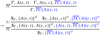
As we mentioned earlier, cyclic proofs of $\mathsf H\textsf{TC}$ indeed are at least as expressive as those of Cohen and Rowe’s system by a routine local simulation of rules:

Theorem 4.11

If $\textsf{TC}_G\vdash _ cyc A$ then $\mathsf H\textsf{TC}\vdash _ cyc A$.

Proof Sketch

Let $\mathcal {D}$ be a $\textsf{TC}_G$ cyclic proof. We can convert it to a $\mathsf H\textsf{TC}$ cyclic proof by simply replacing each sequent $A_1, \dots , A_n$ by the hypersequent $\{ A_1\}^{\varnothing },\dots , \{ A_n\}^{\varnothing }$ and applying some local corrections. In what follows, if $\Gamma = A_1, \dots , A_n$, let us simply write ${\varvec{S}}_\Gamma$ for $\{ A_1\}^{\varnothing }, \dots , \{ A_n\}^{\varnothing }$.

• Any $\textsf{id}$ step of $\mathcal {D}$ must be amended as follows:

  

• Any step of $\mathcal {D}$ becomes a correct step of $\mathsf H\textsf{TC}$ or $\mathsf H\textsf{TC}^=$.

• Any step of $\mathcal {D}$ must be amended as follows:

  

• Any $\exists$ step of $\mathcal {D}$ must be amended as follows:

  

• Any $\forall$ step of $\mathcal {D}$ becomes a correct $\forall$ step of $\mathsf H\textsf{TC}$ or $\mathsf H\textsf{TC}^=$.

• Any $TC _0$ step of $\mathcal {D}$ becomes a correct $TC _0$ step of $\mathsf H\textsf{TC}$.

• Any $TC _1$ step of $\mathcal {D}$ must be amended as follows:

  

• Any $\overline{ TC }$ step of $\mathcal {D}$ must be amended as follows:

  

Particular inspection of the $\overline{ TC }$ case shows that progressing traces of $\textsf{TC}_G$ induce progressing hypertraces of $\mathsf H\textsf{TC}$. Also, since each of the cases above maps an inference step of $\textsf{TC}_G$ to a fixed finite gadget in $\mathsf H\textsf{TC}$, regularity is preserved too.

5 Soundness of $\mathsf H\textsf{TC}$

This section is devoted to the proof of the first of our main results:

Theorem 5.1

(Soundness) If $\mathsf H\textsf{TC}\vdash _ nwf$ S then $\models$ S.

The argument is quite technical due to the alternating nature of our progress condition. In particular the treatment of traces within hypertraces requires a more fine grained argument than usual, bespoke to our hypersequential structure.

5.1 Some Conventions on (Pre)proofs and Semantics

First, we work with proofs without substitution, in order to control the various symbols occurring in a proof.

Throughout this section, we shall fix a HTC preproof D of a hypersequent S. We start by introducing some additional definitions and propositions.

Proposition 5.2

If $\mathsf H\textsf{TC}\vdash _ nwf {\varvec{S}}$ then there is also a $\mathsf H\textsf{TC}$ proof of ${\varvec{S}}$ that does not use the substitution rule.

Proof Sketch

We appeal to a coinductive argument, applying a meta-level substitution operation on proofs to admit each substitution step. Productivity of the translation is guaranteed by the progressing condition: each infinite branch must, at the very least, have infinitely many $\overline{ TC }$ steps.

The utility of this is that we can now carefully control the occurrences of eigenfunctions in a proof so that, bottom-up, they are never ‘re-introduced’, thus facilitating the definition of interpretations on them.

Throughout this section, we shall allow interpretations to be only partially defined, i.e. they are now partial maps from the set of function symbols of our language to appropriately typed functions in the structure at hand. Typically our interpretations will indeed interpret the function symbols in the context in which they appear, but as we consider further function symbols it will be convenient to extend an interpretation ‘on the fly’. This idea is formalised in the following definition:

Definition 5.3

(Interpretation extension) Let $\mathcal {M}$ be a structure and $\rho$, $\rho '$ be two (partial) interpretations over $\mid \!\!\mathcal {M}\!\!\mid$. We say that $\rho '$ is an extension of $\rho$, written $\rho \subseteq \rho '$, if $\rho '(f) = \rho (f)$, for all f in the domain of $\rho$.

Finally, we assume that the free and bound variables occurring in a hypersequent at the root a (pre)proof are all pairwise distinct, and that whenever we apply rule $\exists$ or rule $TC$ (resp. rule $\forall$ or rule $\overline{ TC }$) to a hypersequent ${\varvec{S}}$ occurring in a branch, the rule introduces in the premiss a variable (resp. a function symbol) that does not appear in any hypersequent in the branch from the root up to ${\varvec{S}}$, included. This strong freshness requirement guarantees that each function and variable symbol is uniquely interpreted in the countermodel that we are going to construct.

5.2 Constructing a ‘Countermodel’ Branch

Recall that we have fixed at the beginning of this section a $\mathsf H\textsf{TC}$ preproof $\mathcal {D}$ of a hypersequent ${\varvec{S}}$. Let us fix some structure $\mathcal {M}^\times$ and an interpretation $\rho _0$ such that $\rho _0 \not \models {\varvec{S}}$ (within $\mathcal {M}^\times$). As we shall prove in the following Lemma, since each rule is locally sound, by contraposition we can continually choose ‘false premisses’ to construct an infinite ‘false branch’:

Lemma 5.4

(Countermodel branch) There is a branch $\mathcal {B}^\times = ({\varvec{S}}_i)_{i < \omega }$ of $\mathcal {D}$ and an interpretation $\rho ^\times$ such that, with respect to $\mathcal {M}^\times$:

• 1. $\rho ^\times \not \models {\varvec{S}}_i$, for all $i<\omega$;

• 2. Suppose that ${\varvec{S}}_i$ concludes a $\overline{ TC }$ step, as typeset in Fig. 4, and $\rho ^\times \models TC ({\bar{A}})(s,t) \, [{\textbf {d}}/{\textbf {x}}]$. If n is minimal such that $\rho ^\times \models \bar{A}(d_i,d_{i+1})$ for all $i< n$, $\rho ^\times (s)=d_0$ and $\rho ^\times (t)=d_n$, and $n>1$, then $\rho ^\times (f)({\textbf {d}}) = d_1$,³ so that $\rho ^\times \models \bar{A}(s,f({\textbf {x}})) [{\textbf {d}}/{\textbf {x}}]$, and $\rho ^\times \models TC ({\bar{A}})(f({\textbf {x}}),t) [{\textbf {d}}/{\textbf {x}}]$.

Intuitively, our interpretation $\rho ^\times$ is going to be defined as the limit of a chain of ‘partial’ interpretations $(\rho _i)_{i<\omega }$, with each $\rho _i \not \models {\varvec{S}}_i$ (with respect to $\mathcal {M}^\times$). Referring to Item 2, whenever some $\overline{ TC }$-formula is principal, we shall always choose $\rho _{i+1}$ to assign to it a falsifying path of minimal length (if one exists at all), with respect to an assignment ${\textbf {d}}$ to variables ${\textbf {x}}$ in the annotation of its cedent. It is crucial at this point that our definition of $\rho ^\times$ is parametrised by such assignments.

Proof of Lemma 5.4

We construct $\mathcal {B}^\times$ and $\rho ^\times$ simultaneously. In fact we shall define a chain of interpretations $\rho _0 \subseteq \rho _1\subseteq \rho _2 \subseteq \cdots$ such that, for each i, $\mathcal {M}^\times , \rho _i \models {\varvec{S}}_i$. We will define $\rho ^\times$ as the limit of this chain. We distinguish cases according to the rule $\mathsf r_i$ that ${\varvec{S}}_i$ concludes. For the case of weakening, ${\varvec{S}}_{i+1}$ is the unique premiss of the rule, and $\rho _{i+1} = \rho _i$. We now give all the other cases:

$\triangleright$ Case $(\cup )$

By assumption, $\rho _i \not \models {\textbf {Q}}$ and . Set $\rho _{i+1} = \rho _i$. By the truth condition for $\forall$, we have that for all m-tuples ${\textbf {d}}_1 \in \mid \!\!\mathcal {M}^\times \!\!\mid$ and n-tuples ${\textbf {d}}_2 \in \mid \!\!\mathcal {M}^\times \!\!\mid$, for $n = \mid \!{\textbf {x}}_1 \! \mid$, $m = \mid \!{\textbf {x}}_2 \! \mid$:

By the truth condition associated to we can conclude that, for all ${\textbf {d}}_1$, ${\textbf {d}}_2$, either:

$$\begin{aligned} \rho _{i+1} \models \bigvee \overline{\Gamma }_1 \quad [{\textbf {d}}_1 / {\textbf {x}}_1][{\textbf {d}}_2 / {\textbf {x}}_2] \quad \text { or } \quad \rho _{i+1} \models \bigvee \overline{\Gamma }_2\quad [{\textbf {d}}_1 / V_1][{\textbf {d}}_2 / V_2]. \end{aligned}$$

Since ${\textbf {x}}_1 \cap \textsf{fv}(\Gamma _2) = \varnothing$ and ${\textbf {x}}_2 \cap \textsf{fv}(\Gamma _1)=\varnothing$, the above is equivalent to:

$$\begin{aligned} \rho _{i+1} \models \bigvee \overline{\Gamma }_1 \quad [{\textbf {d}}_1 / {\textbf {x}}_1] \quad \text { or } \quad \rho _{i+1} \models \bigvee \overline{\Gamma }_2\quad [{\textbf {d}}_2 / {\textbf {x}}_2]. \end{aligned}$$

And, since this holds for all choices of ${\textbf {d}}_1$ and ${\textbf {d}}_2$, we can conclude that:

$$\begin{aligned} \rho _{i+1}\models \forall {\textbf {x}}_1( \bigvee \overline{\Gamma }_1) \quad \text { or } \quad \rho _{i+1} \models \forall {\textbf {x}}_2( \bigvee \overline{\Gamma }_2). \end{aligned}$$

Take ${\varvec{S}}_{i+1}$ to be the ${\varvec{S}}^k$ such that $\rho _{i+1} \models \forall {\textbf {x}}_k( \bigvee \overline{\Gamma }_k)$, for $k = \{1,2\}$.

For all the remaining cases, ${\varvec{S}}_{i+1}$ is the unique premiss of the rule $\mathsf r_i$. Moreover, for ${\textbf {x}}$ the unique (possibly empty) annotation explicitly indicated in the remaining rules, let $n = \mid \!{\textbf {x}} \! \mid$ and ${\textbf {d}}\in \mid \!\!\mathcal {M}^\times \!\!\mid ^n$.

$\triangleright$ Cases , , $(\exists )$, $(\textsf{id})$ and $( TC )$

For all these cases set $\rho _{i+1} = \rho _i$. The formula interpretation of the conclusion logically implies the formula interpretation of the premiss. Thus, from $\mathcal {M}^\times , \rho _{i} \not \models {\varvec{S}}_i$ we have that $\mathcal {M}^\times , \rho _{i+1} \not \models {\varvec{S}}_{i+1}$. Let us justify this explicitly for the cases $(\exists )$, $(\textsf{id})$ and $( TC )$. $(\exists )$ By assumption, $\rho _i\not \models {\textbf {Q}}$ and . We have $\rho _{i+1}\not \models {\textbf {Q}}$.

By prenexing the quantifier and variable renaming we obtain .

$(\textsf{id})$ By assumption, $\rho _i\not \models {\textbf {Q}}$ and and $\rho _i \models A$. By the truth condition for $\forall$ we have that, for all choices of ${\textbf {d}}$, it holds that:

By the truth condition for , for every choice of ${\textbf {d}}$:

$$\begin{aligned} \rho _{i+1} \models \bigvee \overline{\Gamma } \quad [{\textbf {d}}/ {\textbf {x}}]\quad \text { or } \quad \rho _{i+1} \models \overline{A} \quad [{\textbf {d}}/ {\textbf {x}}]. \end{aligned}$$

Since $\textsf{fv}(A) \cap {\textbf {x}}= \varnothing$, the above is equivalent to:

$$\begin{aligned} \rho _{i+1} \models \bigvee \overline{\Gamma } \quad [{\textbf {d}}/ {\textbf {x}}] \quad \text { or } \quad \rho _{i+1} \models \overline{A}. \end{aligned}$$

By assumption, $\rho _{i+1} \models A$. Thus, the second disjunct cannot hold, and we have that $\rho _{i+1} \models \bigvee \overline{\Gamma } \quad [{\textbf {d}}/ {\textbf {x}}]$. Since this holds for all choices of ${\textbf {d}}$, we conclude that $\rho _{i+1} \models \forall {\textbf {x}}(\bigvee \overline{\Gamma } )$.

$( TC )$ By assumption, $\rho _i\not \models {\textbf {Q}}$ and . Recall that $\overline{ TC ({A})(s,t))} :=\overline{ TC }({\overline{A}})(s,t)$. We reason as follows:

In the above, step $(\star )$ follows from the inductive definition of $\overline{ TC }$, and step $(*)$ is obtained by distributing $\forall$ over , i.e., by means of the classical theorem . The other steps are either standard theorems or follow from the truth conditions of the logical operators.

For the three remaining cases of $(\textsf{inst})$, $(\forall )$ and $(\overline{ TC })$, $\rho _{i+1}$ extends $\rho _i$ by adequately interpreting the new function symbols introduced, bottom-up:

$\triangleright$ Case $(\textsf{inst})$

By assumption, $\rho _i\not \models {\textbf {Q}}$ and $\rho _i \models \forall {\textbf {x}}\, \forall x( \bigvee \overline{\Gamma }(x))$. Thus, for all choices of ${\textbf {d}}$, we have that $\rho _{i} \models \forall x (\bigvee \overline{\Gamma }(x)) \, [{\textbf {d}}/ {\textbf {x}}]$. By the truth condition for $\forall$, this means that, for all $d \in \mid \!\!\mathcal {M}^\times \!\!\mid$, $\rho _{i} \models \bigvee \overline{\Gamma }(x) \, [{\textbf {d}}/ {\textbf {x}}] [d / x]$. Take $\rho _{i+1}$ to be any extension of $\rho _i$ that is defined on the language of ${\varvec{S}}_{i+1}$. That is, if f is a function symbol in t to which $\rho _{i}$ already assigns a map, then $\rho _{i+1}$ assigns to it that same map. Otherwise, $\rho _{i+1}$ assigns an arbitrary map to f.

It follows that $\rho _{i+1}\not \models fm ({\textbf {Q}})$ and $\rho _{i+1} \models \bigvee \overline{\Gamma }(t) [{\textbf {d}}/ {\textbf {x}}]$ and, since this holds for all ${\textbf {d}}$, we have that $\rho _{i+1} \models \forall {\textbf {x}}( \bigvee \overline{\Gamma }(t))$. Thus $\rho _{i+1} \not \models {\varvec{S}}_{i+1}$.

$\triangleright$ Case $(\forall )$

By assumption, $\rho _i\not \models {\textbf {Q}}$ and . By the truth condition for $\forall$ and , for all choices of ${\textbf {d}}$ we have:

$$\begin{aligned} \rho _i \models \bigvee \overline{\Gamma } \quad [{\textbf {d}}/ {\textbf {x}}] \quad \text { or } \quad \rho _i \models \exists x(\overline{A}(x)) \quad [{\textbf {d}}/ {\textbf {x}}]. \end{aligned}$$

We define $\rho _{i+1}$ to extend $\rho _i$ by defining $\rho _{i+1}(f)$ as follows. Let ${\textbf {d}} \subseteq \mid \!\!\mathcal {M}^\times \!\!\mid$. If $\rho _{i} \models \bigvee \overline{\Gamma } \, [{\textbf {d}}/ {\textbf {x}}]$ then we may set $\rho _{i+1}(f)({\textbf {d}})$ to be arbitrary. We still have $\rho _{i+1} \models \bigvee \overline{\Gamma } \, [{\textbf {d}}/{\textbf {x}}]$, as required. Otherwise $\rho _i \models \exists x(\overline{A}(x)) \, [{\textbf {d}}/ {\textbf {x}}]$. By the truth condition for $\exists$, there is a $d \in \mid \!\!\mathcal {M}^\times \!\!\mid$ such that $\rho _i \models \overline{A}(x) \, [{\textbf {d}}/ {\textbf {x}}][d / x]$. In this case, we define $\rho _{i+1}(f) ({\textbf {d}}) =d$, so that $\rho _{i+1} \models \overline{A}(f({\textbf {x}})) \, [{\textbf {d}}/ {\textbf {x}}]$. So, for all ${\textbf {d}}$, we have that , and so . Thus, $\rho _{i+1} \not \models {\varvec{S}}_{i+1}$, as required.

$\triangleright$ Case $(\overline{ TC })$

By assumption, $\rho _i\not \models {\textbf {Q}}$ and which, by definition of duality, means . By the truth conditions for we have, for all ${\textbf {d}}$:

$$\begin{aligned} 1) \quad \rho _{i} \models \bigvee \overline{\Gamma } \, [{\textbf {d}}/ {\textbf {x}}] \quad \text { or } \quad 2) \quad \rho _i \models TC ({\bar{A}})(s,t) \, [{\textbf {d}}/{\textbf {x}}]. \end{aligned}$$

We define $\rho _{i+1}$ to extend $\rho _{i}$ by defining $\rho _{i+1}(f)$ as follows. Let ${\textbf {d}}\subseteq \mathcal {M}^\times$. If 1) holds, then we may set $\rho _{i+1}(f)({\textbf {d}})$ to be an arbitrary element of $\mid \!\!\mathcal {M}^\times \!\!\mid$. Otherwise, 2) must hold, so by the truth conditions for $TC$ there is a $\overline{A}$-path between $\rho _{i}(s)$ and $\rho _{i}(t)$ of length greater or equal than 1, i.e. there are elements $d_0, \dots , d_{n}$, with $n>0$ and $\rho _i(s)=d_0$ and $\rho _i(t)=d_{n}$, such that $\rho _i \models \bar{A}(d_i,d_{i+1})$ for all $i< n$. We select a shortest such path, i.e. one with smallest possible $n>0$. There are two cases:

• (i) if $n=1$, then already $\rho _i \models \bar{A}(s,t) [{\textbf {d}}/{\textbf {x}}]$, so we may set $\rho _{i+1}(f)({\textbf {d}})$ to be arbitrary;

• (ii) otherwise $n>1$ and we set $\rho _{i+1}(f)({\textbf {d}}) = d_1$, so that $\rho _{i+1} \models \bar{A}(s,f({\textbf {x}})) [{\textbf {d}}/{\textbf {x}}]$ and $\rho _{i+1} \models TC ({\bar{A}})(f({\textbf {x}}),t) [{\textbf {d}}/{\textbf {x}}]$.

We have considered all the rules, so the construction of $\mathcal {B}^\times$ and the all $\rho _i$’s is complete. From here, note that we have $\rho _i \subseteq \rho _{i+1}$, for all $i<\omega$. Thus we can construct the limit $\rho ^\times = \bigcup _{i<\omega } \rho _i$.

5.3 Canonical Assignments Along Countermodel Branches

Let us now fix $\mathcal {B}^\times$ and $\rho ^\times$ as provided by Lemma 5.4 above. Moreover, let us henceforth assume that $\mathcal {D}$ is a proof, i.e. it is progressing, and fix a progressing hypertrace $\mathcal {H}= (\{ \Gamma _i\}^{{\textbf {x}}_i})_{i< \omega }$ along $\mathcal {B}^\times$. In order to carry out an infinite descent argument, we will need to define a particular trace along this hypertrace that ‘preserves’ falsity, bottom-up. This is delicate since the truth values of formulas in a trace depend on the assignment of elements to variables in the annotations. A particular issue here is the instantiation rule $\textsf{inst}$, which requires us to ‘revise’ whatever assignment of y we may have defined until that point. Thankfully, our earlier convention on substitution-freeness and freshness of the variables introduced by quantifiers and transitive closure rules in $\mathcal {D}$ facilitates the convergence of this process to a canonical such assignment:

Definition 5.5

(Assignment) We define $\delta _\mathcal {H}: \bigcup \limits _{i<\omega }{\textbf {x}}_i \rightarrow \mid \!\!\mathcal {M}^\times \!\!\mid$ by $\delta _\mathcal {H}(x) :=\rho (t)$ if x is instantiated by t in $\mathcal {H}$; otherwise $\delta _\mathcal {H}(x)$ is some arbitrary $d\in \mid \!\!\mathcal {M}^\times \!\!\mid$.

Note that $\delta _\mathcal {H}$ is indeed well-defined, thanks to the convention that each quantifier and transitive closure rule introduces only variables that do not appear in previous sequents in the derivation branch. In particular we have that each variable x is instantiated at most once along a hypertrace. Henceforth we shall simply write $\rho ,\delta _\mathcal {H}\models A({\textbf {x}})$ instead of $\rho \models A(\delta _\mathcal {H}({\textbf {x}}))$. Working with such an assignment ensures that false formulas along $\mathcal {H}$ always have a false immediate ancestor:

Lemma 5.6

(Falsity through $\mathcal {H}$) If $\rho ^\times , \delta _\mathcal {H}\not \models F$ for some $F\in \Gamma _i$, then F has an immediate ancestor $F'\in \Gamma _{i+1}$ with $\rho ^\times ,\delta _\mathcal {H}\not \models F'$.

Proof

Suppose that F is a formula occurring in some cedent $\{ \Gamma _i\}^{{\textbf {x}}_i}$ in ${\varvec{S}}_i$, such that $\rho ^\times , \delta _\mathcal {H}\not \models F$. We show how to choose a $F'$ satisfying the conditions of the Lemma. We distinguish cases according to the rule $\mathsf r_i$ that $\{ \Gamma _i\}^{{\textbf {x}}_i}$ concludes. Propositional cases are routine as well as $\cup$, since the failed branch has been chosen during the construction of $\mathcal {B}^\times$. For the weakening rule, observe that we could not have chosen a hypertrace going through the structure which gets weakened, as by assumption the hypertrace is infinite. We show the remaining cases. It can be easily checked that, given a formula F such that $\rho ^\times , \delta _\mathcal {H}\not \models F$, the formula $F'$ is an immediate ancestor of F.

$\triangleright$ Case $(\exists )$. Suppose $\{ \Gamma _i\}^{{\textbf {x}}_i} = \{ \Gamma , \exists x (A(x))\}^{{\textbf {x}}}$ and $\{ \Gamma _{i+1}\}^{{\textbf {x}}_{i+1}} = \{ \Gamma ,A(y)\}^{{\textbf {x}},y}$. By assumption, . By the truth condition for $\forall$ we obtain that, for all n-tuples ${\textbf {d}}$ of elements of $\mid \!\!\mathcal {M}^\times \!\!\mid$, for $n = \mid \!{\textbf {x}} \! \mid$, it holds that:

(5)

By definition, $\delta _\mathcal {H}$ assigns a value in the domain to all the variables occurring in annotations along $\mathcal {H}$. From (5) and the truth condition for it follows that:

$$\begin{aligned} \rho ^\times , \delta _\mathcal {H}\models \bigvee \overline{\Gamma } \quad \text { or } \quad \rho ^\times , \delta _\mathcal {H}\models \forall x (\overline{A}(x)). \end{aligned}$$

If $F \in \Gamma$, by hypothesis we have that $\rho ^\times , \delta _\mathcal {H}\models \overline{F}$ and we set $F' = F$. Otherwise, $F = \exists x (A(x))$ and $\rho ^\times , \delta _\mathcal {H}\models \forall x (\overline{A}(x))$. By the truth condition for $\forall$ we have $\rho ^\times , \delta _\mathcal {H}\models \overline{A}(y)$, so we set $F' = A(y)$.

$\triangleright$ Case $(\textsf{inst})$. Suppose $\{ \Gamma _i\}^{{\textbf {x}}_i} = \{ \Gamma (y)\}^{{\textbf {x}},y}$ and $\{ \Gamma _{i+1}\}^{{\textbf {x}}_{i+1}} = \{ \Gamma (t)\}^{{\textbf {x}}}$. By construction, $\rho ^\times \models \forall {\textbf {x}}\, \forall y( \bigvee \overline{\Gamma }(y))$. Reasoning as in the previous case, from the truth condition for $\forall$ it follows that $\rho ^\times , \delta _\mathcal {H}\models \bigvee \overline{\Gamma }(y)$. If F does not contain y, then $\rho ^\times , \delta _\mathcal {H}\models \overline{F}$, and we set $F' = F$. Otherwise, if F contains y, then $\rho ^\times , \delta _\mathcal {H}\models \overline{F}(y)$. By Lemma 5.4, $\rho ^\times$ assigns a value to t, and by Definition 5.5, since y is instantiated with t along $\mathcal {H}$, $\delta _\mathcal {H}(y) = \rho ^\times (t)$. Therefore we have $\rho ^\times , \delta _\mathcal {H}\models \overline{F}(t)$ so we set $F' = F(t)$.

$\triangleright$ Case $(\textsf{id})$. Suppose $\{ \Gamma _i\}^{{\textbf {x}}_i} = \{ \Gamma , A\}^{{\textbf {x}}}$ and $\{ \Gamma _{i+1}\}^{{\textbf {x}}_{i+1}} = \{ \Gamma \}^{{\textbf {x}}}$. Observe that the hypertrace $\mathcal {H}$ could not have gone through the structure occurring in the conclusion of the rule, because by assumption $\mathcal {H}$ is infinite. Moreover, by construction the formula interpretation of all the cedents along $\mathcal {B}^\times$ is not valid, and thus . This implies that $\rho ^\times \models A$ and so:

$$\begin{aligned} \rho ^\times , \delta _\mathcal {H}\models \bigvee \overline{\Gamma }. \end{aligned}$$

So we have that $F\in \Gamma$ and $\rho ^\times , \delta _\mathcal {H}\models \overline{F}$. Set $F' = F$.

$\triangleright$ Case $( TC )$. Suppose $\{ \Gamma _i\}^{{\textbf {x}}_i} = \{ \Gamma , TC ({A})(s,t)\}^{{\textbf {x}}}$. By assumption, . Thus, we have that:

$$\begin{aligned} \rho ^\times , \delta _\mathcal {H}\models \bigvee \overline{\Gamma } \, \text { or } \, \rho ^\times , \delta _\mathcal {H}\models \overline{ TC }({\overline{A}})(s,t). \end{aligned}$$

From the inductive definition of $\overline{ TC }$ and the truth condition for , the second disjunct is equivalent to:

(6)

There are two cases to consider, since the premiss of the rule has two cedents that the hypertrace $\mathcal {H}$ could follow:

• (i) $\{ \Gamma _{i+1}\}^{{\textbf {x}}_{i+1}} = \{ \Gamma , A(s,t)\}^{{\textbf {x}}}$. By construction, , and thus . If $F \in \Gamma$, then $\rho ^\times , \delta _\mathcal {H}\models \overline{F}$. Set $F = F'$. Otherwise, $F = TC ({A})(s,t)$ and $\rho ^\times , \delta _\mathcal {H}\models \overline{F}$. By (6) we have that $\rho ^\times , \delta _\mathcal {H}\models \overline{A}(s,t)$. Set $F' = A(s,t)$.

• (ii) $\{ \Gamma _{i+1}\}^{{\textbf {x}}_{i+1}} = \{ \Gamma , A(s,z), TC ({A})(z,t)\}^{{\textbf {x}},z}$. By construction, we have that . Since z does not occur free in $\Gamma$, this is equivalent to . If $F \in \Gamma$ and $\rho ^\times , \delta _\mathcal {H}\models \overline{F}$, set $F' = F$. Suppose $F = TC ({A})(s,t)$ and $\rho ^\times , \delta _\mathcal {H}\models \overline{F}$. From (6) we have:

  

  If $\rho ^\times , \delta _\mathcal {H}\models \overline{A}(s,z)$, set $F' = A(s,z)$. Otherwise, if $\rho ^\times , \delta _\mathcal {H}\models \overline{ TC }({A})(z,t)$, set $F'= TC ({A})(z,t)$.

$\triangleright$ Case $(\forall )$. Suppose $\{ \Gamma _i\}^{{\textbf {x}}_i} = \{ \Gamma , \forall x (A(x))\}^{{\textbf {x}}}$ and $\{ \Gamma _{i+1}\}^{{\textbf {x}}_{i+1}} = \{ \Gamma ,A(f({\textbf {x}}))\}^{{\textbf {x}}}$. By assumption, and, from the truth conditions for $\forall$ and :

$$\begin{aligned} \rho ^\times , \delta _\mathcal {H}\models \bigvee \overline{\Gamma } \quad \text { or } \quad \rho ^\times , \delta _\mathcal {H}\models \exists x (\overline{A}(x)). \end{aligned}$$

If $F \in \Gamma$ and $\rho ^\times , \delta _\mathcal {H}\models \overline{F}$, set $F' = F$, since x does not occur in $\Gamma$. Otherwise, $F = \forall x(A (x))$ and $\rho ^\times , \delta _\mathcal {H}\models \exists x (\overline{A}(x))$. By definition of $\rho ^\times$ and $\delta _\mathcal {H}$ we have $\rho ^\times , \delta _\mathcal {H}\models \overline{ A}(f({\textbf {x}}))$, so we set $F' = A(f({\textbf {x}}))$.

$\triangleright$ Case $(\overline{ TC })$. Suppose $\{ \Gamma _i\}^{{\textbf {x}}_i} = \{ \Gamma , \overline{ TC }({A})(s,t)\}^{{\textbf {x}}}$. By assumption, , that is, . Thus, we have that:

$$\begin{aligned} \rho ^\times , \delta _\mathcal {H}\models \bigvee \overline{\Gamma } \quad \text { or } \quad \rho ^\times , \delta _\mathcal {H}\models TC ({\overline{A}})(s,t). \end{aligned}$$

We need to consider two cases, depending on which cedent the hypertrace $\mathcal {H}$ follows:

• (i) $\{ \Gamma _{i+1}\}^{{\textbf {x}}_{i+1}} = \{ \Gamma , A(s,t), A(s, f({\textbf {x}})) \}^{{\textbf {x}}}$. If $F \in \Gamma$ set $F = F'$. By assumption it follows that $\rho ^\times , \delta _\mathcal {H}\models \overline{F}$. Otherwise, $F = \overline{ TC }({ A})(s,t)$ and by assumption $\rho ^\times , \delta _\mathcal {H}\models TC ({\overline{A}})(s,t)$. By the inductive definition of $TC$ and the truth condition for , this is equivalent to:

  

  If $\rho ^\times , \delta _\mathcal {H}\models \overline{A}(s,t)$, set $F' = A(s,t)$. Otherwise, . Let $\delta _\mathcal {H}({\textbf {x}}) = {\textbf {d}}$. According to the definition of $\rho ^\times$ at the $(\overline{ TC })$ step, since $\rho ^\times , \delta _\mathcal {H}\not \models \bigvee \overline{\Gamma }$ and $\rho ^\times , \delta _\mathcal {H}\not \models \overline{A}(s,t)$, then $\rho ^\times (f)({\textbf {d}})$ is defined as in case 2), subcase (ii). Thus, $\rho ^\times (f)({\textbf {d}})$ is an element $d \in \mid \!\!\mathcal {M}^\times \!\!\mid$ such that $\rho ^\times , \delta _\mathcal {H}\models \overline{A}(s,f({\textbf {x}}))$ and $\rho ^\times , \delta _\mathcal {H}\models TC ({\overline{A}})(f({\textbf {x}}),t)$. Set $F' = A(s,f({\textbf {x}}))$.

• (ii) $\{ \Gamma _{i+1}\}^{{\textbf {x}}_{i+1}} = \{ \Gamma , A(s,t), \overline{ TC }({A})(f({\textbf {x}}),t)\}^{{\textbf {x}}}$. The proof proceeds exactly as in the previous case except for the very last step, where $F'$ is set to be $\overline{ TC }({A})(f({\textbf {x}}),t)$.

5.4 Putting It All Together

Note how rule $\textsf{inst}$ of Fig. 4 is handled in the proof above: if $F \in \Gamma (y)$ then we can choose $F' = F[t/y]$ which, by definition of $\delta _\mathcal {H}$, has the same truth value. By repeatedly applying Lemma 5.6 we obtain:

Proposition 5.7

(False trace) There exists an infinite trace $\tau ^\times = (F_i)_{i<\omega }$ through $\mathcal {H}$ such that, for all i, it holds that $\mathcal {M}^\times , \rho ^\times , \delta _\mathcal {H}\not \models F_i$.

Proof Sketch

We inductively define $\tau ^\times$ as follows. By assumption, $\mathcal {M}^\times , \rho ^\times \not \models {\varvec{S}}_0$, and thus in particular $\rho ^\times \models \forall {\textbf {x}}_0 (\bigvee \overline{\Gamma }_0)$. Thus, for all n-tuples ${\textbf {d}}$ of elements of $\mid \!\!\mathcal {M}^\times \!\!\mid$, for $n = \mid \!{\textbf {x}}_0 \! \mid$, we have that $\rho ^\times \models \bigvee \overline{\Gamma }_0 \, [{\textbf {d}}/ {\textbf {x}}_0]$. Since $\delta _\mathcal {H}$ assigns a value to all variables occurring in annotations of cedents in $\mathcal {H}$, $\rho ^\times , \delta _\mathcal {H}\models \bigvee \overline{\Gamma }_0$. Take $F_0 \in \Gamma _0$ such that $\mathcal {M}^\times , \rho ^\times , \delta _\mathcal {H}\not \models \overline{F}_0$. From here we define each successive $F_i$ by appealing repeatedly to Lemma 5.6 above.

We are now ready to prove our main soundness result.

Proof of Theorem 5.1

Fix the infinite trace $\tau ^\times = (F_i)_{i<\omega }$ through $\mathcal {H}$ obtained by Proposition 5.7. Since $\tau ^\times$ is infinite, by definition of $\mathsf H\textsf{TC}$ proofs, it needs to be progressing, i.e., it is infinitely often $\overline{ TC }$-principal and there is some $k\in \mathbb N$ s.t. for $i>k$ we have that $F_i = \overline{ TC }({A})(s_i,t_i)$ for some terms $s_i,t_i$.

To each $F_i$, for $i>k$, we associate the natural number $n_i$ measuring the ‘$\bar{A}$-distance between $s_i$ and $t_i$’. Formally, $n_i\in \mathbb N$ is least s.t. there are $d_0, \dots , d_{n_i} \in \mid \!\!\mathcal {M}^\times \!\!\mid$ with $\rho ^\times (s_i) = d_0, \rho ^\times (t_i) = d_{n_i}$ and, for all $i<n_i$, $\rho ^\times ,\delta _\mathcal {H}\models \bar{A}(d_i,d_{i+1})$. Our aim is to show that $(n_i)_{i > k}$ has no minimal element, contradicting wellfoundness of $\mathbb N$. For this, we establish the following two local properties:

• 1. $(n_i)_{i> k}$ is monotone decreasing, i.e., for all $i > k$, we have $n_{i+1}\le n_i$;

• 2. Whenever $F_i$ is principal, we have $n_{i+1} < n_i$.

We prove item 1 and item 2 by inspection on $\mathsf H\textsf{TC}$ rules. We start with item 2. Suppose $F_i = \overline{ TC }({A})(s,t)$ is the principal formula in an occurrence of $\overline{\textsf{tc}}$ so $F_{i+1} = \overline{ TC }({A})(f({\textbf {x}}),t)$, for some ${\textbf {x}}$. Moreover, by construction $\rho ^\times , \delta _\mathcal {H}\models TC ({\overline{A}})(s,t)$ and $\rho ^\times , \delta _\mathcal {H}\models TC ({\overline{A}})(f({\textbf {x}}),t)$. We have to show that $n_i$, the $\overline{A}$-distance between $f({\textbf {x}})$ and t, is strictly smaller than $n_{i+1}$, the $\overline{A}$-distance between s and t, wrt. $\rho ^\times$ and $\delta _\mathcal {H}$.

Let $\delta _\mathcal {H}({\textbf {x}}) = {\textbf {d}}$. By case $(\overline{ TC })$ of Lemma 5.4, and since $\rho ^\times , \delta _\mathcal {H}\models TC ({\overline{A}})(f({\textbf {x}}),t)$, there is a shortest $\overline{A}$-path between $\rho ^\times (s)$ and $\rho ^\times (t)$, composed of $n > 1$ elements $d_0, \dots , d_n$, with $\rho ^\times (s) = d_0$ and $\rho ^\times (t) = d_n$, and $\rho ^\times (f)({\textbf {d}}) = d_1$. Consequently, it holds that $\rho ^\times , \delta _\mathcal {H}\models \overline{A}(s, f({\textbf {x}}))$ and $\rho ^\times , \delta _\mathcal {H}\models TC ({\overline{A}})( f({\textbf {x}}),t)$. Thus, there is an $\overline{A}$-edge between $\rho ^\times (s)$ and $\rho ^\times (f)({\textbf {d}})$, and $\rho ^\times (f)({\textbf {d}})$ is one edge closer to $\rho ^\times (t)$ in one of the shortest $\overline{A}$-paths between $\rho ^\times (s)$ and $\rho ^\times (t)$. We conclude that $n_{i+1}$ is exactly $n_i -1$, and $n_{i+1} < n_i$.

To prove item 1, suppose that $F_i$ is not principal in the occurrence $r_i$ of a $\mathsf H\textsf{TC}$ rule. Suppose $\mathsf r_i$ is $\textsf{inst}$, $F_i = \overline{ TC }({A})(s,x)$, $F_{i+1} = \overline{ TC }({A})(s,t)$, and x gets instantiated with t by $\textsf{inst}$. By construction, $\rho ^\times , \delta _\mathcal {H}\models TC ({\overline{A}})(s,x)$. Let $n_i$ be the distance between $\rho ^\times (s)$ and $\delta _\mathcal {H}(x)$. By definition, $\delta _\mathcal {H}(x) = \rho ^\times (t)$. Thus, the distance between $\rho ^\times (s)$ and $\rho ^\times (t)$ is $n_{i+1} = n_i$. In all the other cases, $F_i = \overline{ TC }({A})(s,t) = F_{i+1}$, and thus $n_{i+1} = n_i$.

So $(n_i)_{i > k}$ is monotone decreasing by item 1 but cannot converge by item 2, and by definition of progressing trace. Thus $(n_i)_{k <i}$ has no minimal element, yielding the required contradiction.

6 Completeness for $\text {PDL}^+$, Over the Standard Translation

In this section we give our next main result:

Theorem 6.1

(Completeness for $\text {PDL}^+$) For a $\text {PDL}^+$ formula A, if $\models A$ then $\mathsf H\textsf{TC}\vdash _ cyc \textsf{ST}(A)({c})$.

The proof is by a direct simulation of a cut-free cyclic system for $\text {PDL}^+$ that is complete. We shall briefly sketch this system below.

6.1 Cyclic System for $\text {PDL}^+$

The system $\textsf{L}\textsf{PD}^+$, shown in Fig. 5, is the natural extension of the usual sequent calculus for basic multimodal logic K by rules for programs. In Fig. 5, $\Gamma ,\Delta$ etc. range over sets of $\text {PDL}^+$ formulas, and we write $\langle a\rangle \Gamma$ as a shorthand for $\{\langle a\rangle B: B \in \Gamma \}$. (Regular) preproofs for this system are defined just like for $\mathsf H\textsf{TC}$ or $\textsf{TC}_G$.

Fig. 5

Rules of $\textsf{L}\textsf{PD}^+$

The notion of ancestry for formulas is colour-coded in Fig. 5 as before: a formula C in a premiss is an immediate ancestor of a formula $C'$ in the conclusion if they have the same colour; if $C,C'\in \Gamma$ then we furthermore require $C=C'$. More formally (and without relying on colours):

Definition 6.2

(Immediate ancestry) Fix a preproof $\mathcal {D}$. We say that a formula occurrence C is an immediate ancestor of a formula occurrence D in $\mathcal {D}$ if C and D occur in a premiss and the conclusion, respectively, of an inference step $\mathsf r$ of $\mathcal {D}$ and:

• If $\mathsf r$ is a $k_a$ step then, as typeset in Fig. 5:

  • D is $\langle a\rangle B$ for some $B\in \Gamma$ and C is B; or,

  • D is $[a] A$ and C is A.

• If $\mathsf r$ is not a k-step then:

  • C and D are occurrences of the same formula; or,

  • D is principal and C is auxiliary in $\mathsf r$, i.e. as typeset in Fig. 5, C and D are the (uniquely) distinguished formulas in a premiss and conclusion, respectively;

Definition 6.3

(Non-wellfounded proofs) Fix a preproof $\mathcal {D}$ of a sequent $\Gamma$. A thread is a maximal path in its graph of immediate ancestry. We say a thread is progressing if it has a smallest infinitely often principal formula of the form $[\alpha ^+]A$.

$\mathcal {D}$ is a proof if every infinite branch has a progressing thread. If $\mathcal {D}$ is regular, we call it a cyclic proof and we may write $\textsf{L}\textsf{PD}^+\vdash _ cyc \Gamma$.

Soundness of cyclic-$\textsf{L}\textsf{PD}^+$ is established by a standard infinite descent argument, but is also implied by the soundness of cyclic-$\mathsf H\textsf{TC}$ (Theorem 5.1) and the simulation we are about to give (Theorem 6.1), though this is somewhat overkill. Completeness may be established by the game theoretic approach of Niwinskí and Walukiewicz [24], as carried out by Lange in [21], or by the purely proof theoretic techniques of Studer [27]. Either way, both results follow immediately by a standard embedding of $\text {PDL}^+$ into the (guarded) $\mu$-calculus and its known completeness results [24, 27], by way of a standard ‘proof reflection’ argument: $\mu$-calculus proofs of the embedding are ‘just’ step-wise embeddings of $\textsf{L}\textsf{PD}^+$ proofs.

Theorem 6.4

(Soundness and completeness, essentially from [21]) Let A be a $\text {PDL}^+$ formula. $\models A$ iff $\textsf{L}\textsf{PD}^+\vdash _ cyc A$.

6.2 Examples of Cyclic Proofs in $\textsf{L}\textsf{PD}^+$

Before giving our main simulation result, let us first see some examples of proofs in $\textsf{L}\textsf{PD}^+$, in particular addressing the ‘counterexample’ from Sect. 3.3.

Example 6.5

Below is a cyclic $\textsf{L}\textsf{PD}^+$ proof of the $\textsf{L}\textsf{PD}^+$ sequent:

$$\begin{aligned}{}[(aa\cup aba)^+] \overline{p}, \langle a^+ \rangle p, \langle (ba^+)^+ \rangle p, \langle a^+\rangle \langle (ba^+)^+ \rangle p. \end{aligned}$$

We use the following abbreviations: $\alpha =(aa\cup aba)^+$ and $\beta = (ba^+)^+$. Moreover, we sometimes use rule $\langle +\rangle$, which is derivable from rules $\langle +\rangle _0$ and $\langle +\rangle _1$, keeping in mind that $\textsf{L}\textsf{PD}^+$ sequents are sets of formulas:

Similarly for rule . There are uncountably many infinite branches, but each such branch is supported by the infinite thread induced by the blue-coloured formulas. $\Gamma$ is sequent $[aa \cup aba] \overline{p}, \langle a^+ \rangle p, \langle \beta \rangle p, \langle a^+\rangle \langle \beta \rangle p$, derivable by means of a finite derivation (which we do not show).

Example 6.6

Below we give a cyclic $\textsf{L}\textsf{PD}^+$ proof of formula (2), which witnesses the incompleteness of $\textsf{TC}_G$ without cut:

$$\begin{aligned} \langle (aa\cup aba)^+\rangle p \, \rightarrow \, \langle a^+((ba^+)^+ \cup a)\rangle p. \end{aligned}$$

We employ the same shorthands as in the previous example, i.e., $\alpha =(aa\cup aba)^+$ and $\beta = (ba^+)^+$. The progressing thread along the unique infinite branch displayed (not including those from Example 6.5), looping on $\bullet$, is coloured blue.

Here $\Gamma '$ is the sequent $[aa \cup aba] \overline{p}, \langle a^+\rangle \langle \beta \cup a\rangle p$, which has a finite derivation:

6.3 A ‘Local’ Simulation of $\textsf{L}\textsf{PD}^+$ by $\mathsf H\textsf{TC}$

In this subsection we show that $\textsf{L}\textsf{PD}^+$-preproofs can be stepwise transformed into $\mathsf H\textsf{TC}$-preproofs, with respect to the standard translation. In order to produce our local simulation, we need a refined version of the standard translation, incorporating the structural elements of hypersequents.

In the definitions below we are often using arbitrarily chosen variables (e.g. “fresh variables”) and constant symbols. We assume these choices do not break our previous assumptions on variables and constants occurring in hypersequents (refer to Sect. 5.1).

Definition 6.7

(Hypersequent translation for formulas) For x a variable and A a $\text {PDL}^+$ formula, we define the hypersequent translation of A, denoted by $\textsf{HT}(A)({c})$, by induction on the complexity of A as follows, for , with d always a fresh constant symbol and y always a fresh variable:

where the cedent translation $\textsf{CT}(B)(t)$ and ${\textbf {x}}_{B}$ are defined as follows:

• if $B = p$ or $B = C \circ D$ or $B = [\beta ]C$, then:

  

• if $B = \langle \beta \rangle C$ then, for z a fresh variable:

  $$\begin{aligned} \textsf{CT}(B)(y) \, :=\, \textsf{ST}(\beta )({y, z}), \textsf{CT}(C)(z) \quad \text {and} \quad {\textbf {x}}_{B} = {\textbf {x}}_{C}, z. \end{aligned}$$

Proposition 6.8

For ${\varvec{S}}$ a hypersequent, and A a $\text {PDL}^+$ formula:

• 1. There is a finite $\mathsf H\textsf{TC}$-derivation from ${\varvec{S}}, \textsf{HT}(A)({c})$ to ${\varvec{S}}, \{ \textsf{CT}(A)(c)\}^{{\textbf {x}}_{A}}$; and,

• 2. There is a finite $\mathsf H\textsf{TC}$-derivation from ${\varvec{S}}, \{ \textsf{CT}(A)(c)\}^{{\textbf {x}}_{A}}$ to .

Proof

By induction on the complexity of A. If A is atomic, a conjunction or a disjunction, then . If $A= [\alpha ] B$, then . If $A = \langle \alpha _1\rangle \dots \langle \alpha _n\rangle B$, for $1 \le n$, then $\{ \textsf{CT}(A)(y)\}^{{\textbf {x}}_{A}} = \textsf{HT}(A)(c)$, and ${\textbf {x}}_{A} = \{y_1, \dots , y_n\}$, for $y_1, \dots , y_n$ variables that do not occur in B. The remaining cases are shown below. The double line in the derivation below denotes $n -1$ occurrences of rules , and $\textsf{IH}$ indicates appeal to the inductive hypothesis.

Definition 6.9

($\textsf{HT}$-translation) Let $\mathcal {D}$ be a $\text {PDL}^+$ preproof. We shall define a $\mathsf H\textsf{TC}$ preproof $\textsf{HT}(\mathcal {D})(c)$ of the hypersequent $\textsf{HT}(A)({c})$ by a local translation of inference steps. Formally speaking, the well-definedness of $\textsf{HT}(\mathcal {D})(c)$ is guaranteed by coinduction: each rule of $\mathcal {D}$ is translated into a (nonempty) derivation.

where (omitted) left-premisses of $\cup$ steps are simply proved by $\textsf{wk},\textsf{id},\textsf{init}$.

where $\mathcal E,\mathcal E'$ derive $\textsf{HT}(\Gamma )({c}), \textsf{HT}([\alpha ]A)({c})$ using $\textsf{wk}$-steps.

By applying the above translation to each rule of a $\text {PDL}^+$ cyclic proof $\mathcal {D}$ of A, we obtain a preproof $\textsf{HT}(\mathcal {D})({c})$ of $\textsf{HT}(A)({c})$. The last step, from $\textsf{HT}(A)({c})$ to $\textsf{ST}(A)({{c}})$, follows from Prop. 6.8.

Remark 6.10

(Deeper inference) Observe that $\mathsf H\textsf{TC}$ can also simulate ‘deeper’ program rules than are available in $\textsf{L}\textsf{PD}^+$.

For example a rule may be simulated too (similarly for $[\, ]$). Thus $\langle a^+\rangle \langle b\rangle p \rightarrow \langle a^+\rangle \langle b\cup c \rangle p$ admits a finite proof in $\mathsf H\textsf{TC}$ (under $\textsf{ST}$), rather than a necessarily infinite (but cyclic) one in $\textsf{L}\textsf{PD}^+$.

6.4 Justifying Regularity and Progress

Proposition 6.11

If $\mathcal {D}$ is regular, then so is $\textsf{HT}(\mathcal {D})(c)$.

Proof sketch

Notice that each step in $\mathcal {D}$ is translated to a finite derivation in $\textsf{HT}(\mathcal {D})(c)$. Thus, if $\mathcal {D}$ has only finitely many distinct subproofs, then also $\textsf{HT}(\mathcal {D})({c})$ has only finitely many distinct subproofs, modulo applications of the substitution rule.

Proposition 6.12

If $\mathcal {D}$ is progressing, then so is $\textsf{HT}(\mathcal {D})(c)$.

Proof sketch

We need to show that every infinite branch of $\textsf{HT}(\mathcal {D})({c})$ has a progressing hypertrace. Since the $\textsf{HT}$ translation is defined stepwise on the individual steps of $\mathcal {D}$, we can associate to each infinite branch $\mathcal B$ of $\textsf{HT}(\mathcal {D})({c})$ a unique infinite branch $\mathcal B'$ of $\mathcal {D}$. Since $\mathcal {D}$ is progressing, let $\tau = (F_i)_{i < \omega }$ be a progressing thread along $\mathcal B'$. By inspecting the rules of $\textsf{L}\textsf{PD}^+$ (and by definition of progressing thread), for some $k\in \mathbb N$, each $F_i$ for $i>k$ has the form: $[\alpha _{i,1}]\cdots [\alpha _{i,n_i}] [\alpha ^+]A,$ for some $n_i \ge 0$. So, for $i>k$, $\textsf{HT}(F_i)(d_i)$ has the form:

By inspection of the $\textsf{HT}$-translation (Definition 6.9) whenever $F_{i+1}$ is an immediate ancestor of $F_i$ in $\mathcal B'$, there is a path from the cedent to the cedent in the graph of immediate ancestry along $\mathcal B$. Thus, since $\tau =(F_i)_{i<\omega }$ is a trace along $\mathcal B'$, we have a (infinite) hypertrace of the form along $\mathcal B$.

By construction $\Delta _i = \varnothing$ for infinitely many $i>k'$, and so $\mathcal H_\tau$ has just one infinite trace. Moreover, by inspection of the $[+]$ step in Definition 6.9, this trace progresses in $\mathcal B$ every time $\tau$ does in $\mathcal B'$, and so progresses infinitely often. Thus, $\mathcal H$ is a progressing hypertrace. Since the choice of the branch $\mathcal B$ of $\mathcal {D}$ was arbitrary, we are done.

6.5 Putting It All Together

We can now finally conclude our main simulation theorem:

Proof of Theorem 6.1

Let A be a $\text {PDL}^+$ formula s.t. $\models A$. By the completeness result for $\textsf{L}\textsf{PD}^+$, Theorem 6.4, we have that $\textsf{L}\textsf{PD}^+\vdash _ cyc A$, say by a cyclic proof $\mathcal {D}$. From here we construct the $\mathsf H\textsf{TC}$ preproof $\textsf{HT}(\mathcal {D})(c)$ which, by Propositions 6.11 and 6.12, is in fact a cyclic proof of $\textsf{HT}(A)(c)$. Finally, we apply Proposition 6.8 to obtain a cyclic $\mathsf H\textsf{TC}$ proof of $\textsf{ST}(A)({c})$.

7 Extension by Equality: Simulating Full $\text {PDL}$

We now briefly explain how our main results are extended to the ‘reflexive’ version of $\text {TCL}$, which we denote by $\text {TCL}^=$, whose language extends that of $\text {TCL}$ by adding atomic formulas of the form $s =t$ and $s \ne t$.

7.1 Hypersequential System with Equality

The calculus $\mathsf H\textsf{TC}^=$ extends $\mathsf H\textsf{TC}$ by the rules:

(7)

The notion of immediate ancestry for formulas and cedents is colour-coded in (7) just as we did for $\mathsf H\textsf{TC}$ in Sect. 4.2. Formally:

Definition 7.1

(Ancestry for cedents, $\mathsf H\textsf{TC}^=$) Let $\mathsf r$ be a $\mathsf H\textsf{TC}^=$ inference step, as typeset in Fig. 4 or (7). We say that a cedent $S$ in a premiss of $\mathsf r$ is an immediate ancestor of a cedent $S'$ in the conclusion of $\mathsf r$ if any of the conditions in Definition 4.2 applies (where in 3. we further ask that $\mathsf r$ is not $\ne$), or the following holds:

• 5. $\mathsf r$ is $\ne$ and $S$ is the (unique) cedent distinguished in the premiss of $\ne$ and $S'$ is the cedent $\{ \Gamma (s), s \ne t\}^{{\textbf {x}}}$ distinguished in the conclusion of $\ne$.

Definition 7.2

(Ancestry for formulas, $\mathsf H\textsf{TC}^=$) Let $\mathsf r$ be a $\mathsf H\textsf{TC}^=$ inference step, as typeset in Fig. 4 or (7). We say that a formula F in a premiss of $\mathsf r$ is an immediate ancestor of a formula $F'$ in the conclusion of $\mathsf r$ if any of the conditions from Definition 4.3 applies, or the following holds:

• (e) $\mathsf r$ is $\ne$ and $F \in \Delta (s)$ and $F'$ is $s \ne t$.

The resulting notions of (pre)proof, (hyper)trace and progress are as in Definition 4.6. Specifically, we have that in rule $=$ as typeset in (7), no infinite trace can include formula $t = t$. Moreover, in rule $\ne$ no infinite trace can include formulas in $\Delta (t)$, while all formulas occurring in $\Delta (s)$ belong to a trace where $s \ne t$ belongs.

Remark 7.3

The simulation of $\textsf{TC}_G$ by $\mathsf H\textsf{TC}$ also extends to their reflexive system $\mathsf R \textsf{TC}_G$, in the presence of equality. For this we must define their operator $RTC ({\lambda x,y.A}) (s,t)$ $:=$ . Semantically, it is correct to set $RTC ({A}) (s,t)$ to be , but this encoding does not lift to the Cohen-Rowe rules for $RTC$.

7.2 Extending the Soundness Argument

Understanding that structures interpret $=$ as true equality, a modular adaptation of the soundness argument for $\mathsf H\textsf{TC}$, cf. Sect. 5, yields:

Theorem 7.4

(Soundness of $\mathsf H\textsf{TC}^=$) If $\mathsf H\textsf{TC}^=\vdash _ nwf {\varvec{S}}$ then $\models {\varvec{S}}$.

Proof Sketch

In the soundness argument for $\mathsf H\textsf{TC}$, in Lemma 5.4, we must further consider cases for equality as follows:

$\triangleright$ Case $(=)$

By assumption, $\rho _{i} \not \models {\textbf {Q}}$ and $\rho _{i} \not \models \{ \Gamma , t = t\}^{{\textbf {x}}}$, i.e., . Since , this is equivalent to $\rho _{i} \models \forall {\textbf {x}}(\bigvee \overline{\Gamma })$. We set $\rho _{i+1} = \rho _{i}$ and conclude that $\rho _{i+1} \not \models \{ \Gamma \}^{{\textbf {x}}}$.

$\triangleright$ Case $(\ne )$

By assumption, $\rho _{i} \not \models {\textbf {Q}}$ and $\rho _{i} \not \models \{ \Gamma (s), s \ne t\}^{{\textbf {x}}}$ and $\rho _{i} \not \models \{ \Delta (t)\}^{{\textbf {x}}}$. Thus,

Set $\rho _{i+1} = \rho _{i}$. If $\rho _{i} \models \forall {\textbf {x}}(\bigvee \overline{\Gamma }(s))$, then , and thus . Otherwise, if $\rho _{i} \models \forall {\textbf {x}}(s = t)$, we can safely substitute term t with term s in the second conjunct, obtaining $\rho _{i+1} \models \forall {\textbf {x}}(\bigvee \overline{\Delta } (s))$. Thus, , and .

For the construction of the ‘false trace’ in Lemma 5.6 we add the following cases for equality:

$\triangleright$ Case $(=)$. Suppose $\{ \Gamma _i\}^{{\textbf {x}}_i} = \{ t = t, \Gamma \}^{{\textbf {x}}}$. By assumption, and thus $\rho ^\times , \delta _\mathcal {H}\models t \ne t$ or $\rho ^\times , \delta _\mathcal {H}\models \bigvee \overline{\Gamma }$. Since the first disjunct cannot hold, the trace cannot follow the formula $t =t$. Thus, if $F = C$ for some C occurring in $\Gamma$ and $\rho ^\times , \delta _\mathcal {H}\models \overline{C}$, set $F' = F$ and conclude that $\rho ^\times , \delta _\mathcal {H}\models \overline{C}$.

$\triangleright$ Case $(\ne )$. The hypertrace $\mathcal {H}$ cannot go through the structure $\{ \Delta (t)\}^{{\textbf {x}}}$, because by hypothesis $\mathcal {H}$ is infinite. Thus, $\{ \Gamma _{i}\}^{{\textbf {x}}_{i}} = \{ \Gamma (s), s \ne t\}^{{\textbf {x}}}$. By assumption, we have that either:

$$\begin{aligned} \rho ^\times , \delta _{\mathcal {H}} \models \bigvee \overline{\Gamma (s)} \quad \text { or } \quad \rho ^\times , \delta _{\mathcal {H}} \models s = t. \end{aligned}$$

If $F = C(s)$ for some C(s) in $\Gamma (s)$ and $\rho ^\times , \delta _{\mathcal {H}} \models \overline{F}$, set $F' = F$. Otherwise, if $\rho ^\times , \delta _{\mathcal {H}} \not \models \bigvee \overline{\Gamma (s)}$, then $\rho ^\times , \delta _{\mathcal {H}} \models s = t$ and F is $s\ne t$. At every occurrence of rule $\ne$ all the formulas occurring in $\Delta (s)$ are immediate ancestors of $s\ne t$. Moreover, by assumption $\rho ^\times \models \forall {\textbf {x}}( \bigvee \overline{\Delta }(t))$. By the truth condition associated to $\forall$ and since ${\textbf {x}}$ is contained in the domain of $\delta _{\mathcal {H}}$, we have that $\rho ^\times , \delta _\mathcal {H}\models \bigvee \Delta (t)$. Since $\rho ^\times , \delta _{\mathcal {H}} \models s = t$, we conclude that $\rho ^\times , \delta _\mathcal {H}\models \bigvee \Delta (s)$. Thus, there exists a $D(s) \in \Delta (s)$ such that $\rho ^\times , \delta _\mathcal {H}\models \bigvee D(s)$. Set $F' = D(s)$.

7.3 Completeness for $\text {PDL}$ (with Tests)

Turning to the modal setting, $\text {PDL}$ may be defined as the extension of $\text {PDL}^+$ by including a program A? for each formula A. Semantically, we have $A?^{\mathcal M} = \{ (v,v): \mathcal M,v\models A \}$. From here we may define $\varepsilon :=\top ?$ and $\alpha ^* :=(\varepsilon \cup \alpha )^+$. Again, while it is semantically correct to set $\alpha ^* = \varepsilon \cup \alpha ^+$, this encoding does not lift to the standard sequent rules for $*$.

The system $\textsf{L}\textsf{PD}$ is obtained from $\textsf{L}\textsf{PD}^+$ by including the rules:

The notion of ancestry for formulas is defined as for $\textsf{L}\textsf{PD}^+$ (Definition 6.2) and colour-coded in the rules. The resulting notions of (pre)proof, thread and progress are as in Definition 6.3. We write $\textsf{L}\textsf{PD}\vdash _ cyc A$ if there is a cyclic proof of A in $\textsf{L}\textsf{PD}$. Just like for $\textsf{L}\textsf{PD}^+$, a standard encoding of $\textsf{L}\textsf{PD}$ into the $\mu$-calculus yields its soundness and completeness, thanks to known sequent systems for the latter, cf. [21, 24, 27].

Theorem 7.5

(Soundness and completeness, essentially from [21]) Let A be a $\text {PDL}$ formula. $\models A$ iff $\textsf{L}\textsf{PD}\vdash _ cyc A$.

Again, a modular adaptation of the simulation of $\textsf{L}\textsf{PD}^+$ by $\mathsf H\textsf{TC}$, cf. Sect. 6, yields:

Theorem 7.6

(Completeness for $\text {PDL}$) Let A be a $\text {PDL}$ formula. If $\models A$ then $\mathsf H\textsf{TC}^=\vdash _ cyc \textsf{ST}(A)({c})$.

Proof sketch

To show completeness, we must add the the cases for the test rules to Definition 6.9:

8 Conclusions

In this work we proposed a novel cyclic system $\mathsf H\textsf{TC}$ for Transitive Closure Logic ($\text {TCL}$) based on a form of hypersequents. We showed a soundness theorem for standard semantics, requiring an argument bespoke to our hypersequents. Our system is cut-free, rendering it suitable for automated reasoning via proof search. We showcased its expressivity by demonstrating completeness for $\text {PDL}$, over the standard translation. In particular, we demonstrated formally that such expressivity is not available in the previously proposed system $\textsf{TC}_G$ of Cohen and Rowe (Theorem 3.7). Our system $\mathsf H\textsf{TC}$ locally simulates $\textsf{TC}_G$ too (Theorem 4.11).

As far as we know, $\mathsf H\textsf{TC}$ is the first cyclic system employing a form of deep inference resembling alternation in automata theory, e.g. wrt. proof checking, cf. Proposition 4.10. It would be interesting to investigate the structural proof theory that emerges from our notion of hypersequent. As hinted at in Example 4.7, $\mathsf H\textsf{TC}$ exhibits more liberal rule permutations than usual sequents, so we expect their focussing and cut-elimination behaviours to similarly be richer, cf. [22, 23].

Finally, our work bridges the cyclic proof theories of (identity-free) $\text {PDL}$ and (reflexive) $\text {TCL}$. With increasing interest in both modal and predicate cyclic proof theory, it would be interesting to further develop such correspondences.

References

Berardi, S., Tatsuta, M.: Classical system of Martin-Lof’s inductive definitions is not equivalent to cyclic proofs. CoRR. http://arXiv.org/abs/1712.09603 (2017)
Blackburn, P., van Benthem, J.: Modal logic: a semantic perspective. In: Blackburn, P., van Benthem, J.F.A.K., Wolter, F. (eds.) Handbook of Modal Logic. Studies in Logic and Practical Reasoning, vol. 3, pp. 1–84. North-Holland, Amsterdam (2007)
Blackburn, P., De Rijke, M., Venema, Y.: Modal Logic, vol. 53. Cambridge University Press, Cambridge (2002)
Bojańczyk, M., Czerwiński, W.: An Automata Toolbox. Lecture Notes. https://www.mimuw.edu.pl/bojan/paper/automata-toolbox-book (2018)
Brotherston, J., Simpson, A.: Sequent calculi for induction and infinite descent. J. Log. Comput. 21(6), 1177–1216 (2011)
Brotherston, J., Distefano, D., Petersen, R.L.: Automated cyclic entailment proofs in separation logic. In: Bjørner, N., Sofronie-Stokkermans, V. (eds.) Automated Deduction—CADE-23—23rd International Conference on Automated Deduction, Wroclaw, Poland, July 31–August 5, 2011. Proceedings. Lecture Notes in Computer Science, Vol. 6803, pp. 131–146. Springer, Berlin (2011). https://doi.org/10.1007/978-3-642-22438-6_12
Brotherston, J., Gorogiannis, N., Petersen, R.L.: A generic cyclic theorem prover. In: Jhala, R., Igarashi, A. (eds.) Programming Languages and Systems—10th Asian Symposium, APLAS 2012, Kyoto, Japan, December 11–13, 2012. Proceedings. Lecture Notes in Computer Science, Vol. 7705, pp. 350–367. Springer, Berlin (2012). https://doi.org/10.1007/978-3-642-35182-2_25
Cohen, L., Rowe, R.N.S.: Uniform inductive reasoning in transitive closure logic via infinite descent. In: Ghica, D.R., Jung, A. (eds.) 27th EACSL Annual Conference on Computer Science Logic, CSL 2018, September 4–7, 2018, Birmingham, UK. LIPIcs, Vol. 119, pp. 17–11716. Schloss Dagstuhl, Leibniz-Zentrum für Informatik (2018). https://doi.org/10.4230/LIPIcs.CSL.2018.17
Cohen, L., Rowe, R.N.S.: Integrating induction and coinduction via closure operators and proof cycles. In: Peltier, N., Sofronie-Stokkermans, V. (eds.) Automated Reasoning—10th International Joint Conference, IJCAR 2020, Paris, France, July 1–4, 2020, Proceedings, Part I. Lecture Notes in Computer Science, Vol. 12166, pp. 375–394. Springer, Berlin (2020). https://doi.org/10.1007/978-3-030-51074-9_21
Cohen, L., Rowe, R.N.: Non-well-founded proof theory of transitive closure logic. ACM Trans. Comput. Logic 21(4), 1–31 (2020)
Das, A.: On the logical complexity of cyclic arithmetic. Log. Methods Comput. Sci. 16, 1 (2020). https://doi.org/10.23638/LMCS-16(1:1)2020
Das, A., Girlando, M.: Cyclic proofs, hypersequents, and transitive closure logic. In: Blanchette, J., Kovács, L., Pattinson, D. (eds.) Automated Reasoning, pp. 509–528. Springer, Cham (2022)
Das, A., Pous, D.: A cut-free cyclic proof system for kleene algebra. In: Automated Reasoning with Analytic Tableaux and Related Methods: 26th International Conference, TABLEAUX 2017, Brasília, Brazil, September 25–28, 2017, Proceedings, pp. 261–277. Springer (2017)
Dax, C., Hofmann, M., Lange, M.: A Proof System for the Linear Time \(\mu \)-Calculus. vol. 4337, pp. 273–284 (2006). https://doi.org/10.1007/11944836_26
Grädel, E.: On transitive closure logic. In: Börger, E., Jäger, G., Büning, H.K., Richter, M.M. (eds.) Computer Science Logic, 5th Workshop, CSL ’91, Berne, Switzerland, October 7–11, 1991, Proceedings. Lecture Notes in Computer Science, vol. 626, pp. 149–163. Springer, Berlin (1991). https://doi.org/10.1007/BFb0023764
Gurevich, Y.: Logic and the Challenge of Computer Science, pp. 1–57. Computer Science Press, Rockville (1988)
Immerman, N.: Languages that capture complexity classes. SIAM J. Comput. 16(4), 760–778 (1987). https://doi.org/10.1137/0216051
Kamareddine, F.D. (ed.): Transitive Closure and the Mechanization of Mathematics, pp. 149–171. Springer, Dordrecht (2003)
Kozen, D.: A completeness theorem for kleene algebras and the algebra of regular events. In: Proceedings of the Sixth Annual Symposium on Logic in Computer Science (LICS ’91), Amsterdam, The Netherlands, July 15–18, 1991, pp. 214–225. IEEE Computer Society, Washington, DC (1991)
Krob, D.: Complete systems of b-rational identities. Theor. Comput. Sci. 89(2), 207–343 (1991). https://doi.org/10.1016/0304-3975(91)90395-I
Lange, M.: Games for modal and temporal logics. PhD thesis (2003)
Marin, S., Miller, D., Volpe, M.: A focused framework for emulating modal proof systems. In: Beklemishev, L.D., Demri, S., Maté, A. (eds.) Advances in Modal Logic 11, Proceedings of the 11th Conference on "Advances in Modal Logic," Held in Budapest, Hungary, August 30–September 2, 2016, pp. 469–488. College Publications, England and Wales. http://www.aiml.net/volumes/volume11/Marin-Miller-Volpe.pdf (2016)
Miller, D., Volpe, M.: Focused labeled proof systems for modal logic. In: Logic for Programming, Artificial Intelligence, and Reasoning, pp. 266–280. Springer (2015)
Niwiński, D., Walukiewicz, I.: Games for the mu-calculus. Theoret. Comput. Sci. 163(1), 99–116 (1996). https://doi.org/10.1016/0304-3975(95)00136-0
Rowe, R.N.S., Brotherston, J.: Automatic cyclic termination proofs for recursive procedures in separation logic. In: Bertot, Y., Vafeiadis, V. (eds.) Proceedings of the 6th ACM SIGPLAN Conference on Certified Programs and Proofs, CPP 2017, Paris, France, January 16–17, 2017, pp. 53–65. ACM, New York (2017). https://doi.org/10.1145/3018610.3018623
Simpson, A.: Cyclic arithmetic is equivalent to peano arithmetic. In: Esparza, J., Murawski, A.S. (eds.) Foundations of Software Science and Computation Structures—20th International Conference, FOSSACS 2017, Held as Part of the European Joint Conferences on Theory and Practice of Software, ETAPS 2017, Uppsala, Sweden, April 22–29, 2017, Proceedings. Lecture Notes in Computer Science, vol. 10203, pp. 283–300 (2017). https://doi.org/10.1007/978-3-662-54458-7_17
Studer, T.: On the proof theory of the modal mu-calculus. Stud. Logica. 89(3), 343–363 (2008)
Tellez, G., Brotherston, J.: Automatically verifying temporal properties of pointer programs with cyclic proof. In: de Moura, L. (ed.) Automated Deduction—CADE 26—26th International Conference on Automated Deduction, Gothenburg, Sweden, August 6–11, 2017, Proceedings. Lecture Notes in Computer Science, vol. 10395, pp. 491–508. Springer, Berlin (2017). https://doi.org/10.1007/978-3-319-63046-5_30
Tellez, G., Brotherston, J.: Automatically verifying temporal properties of pointer programs with cyclic proof. J. Autom. Reason. 64(3), 555–578 (2020)
Thomas, W.: Languages, automata, and logic. In: Rozenberg, G., Salomaa, A. (eds.) Handbook of Formal Languages, pp. 389–455. Springer, Berlin (1997)
Acknowledgements
This work was supported by a UKRI Future Leaders Fellowship, ‘Structure vs Invariants in Proofs’, project reference MR/S035540/1, and by the HORIZON-MSCA-2021-PF-01-01 project ‘CYclic DErivations for Recursive operators’, project ID 101064105.
Author information
Authors and Affiliations
Corresponding author
Additional information
Publisher's Note
Springer Nature remains neutral with regard to jurisdictional claims in published maps and institutional affiliations.
Rights and permissions
Open Access This article is licensed under a Creative Commons Attribution 4.0 International License, which permits use, sharing, adaptation, distribution and reproduction in any medium or format, as long as you give appropriate credit to the original author(s) and the source, provide a link to the Creative Commons licence, and indicate if changes were made. The images or other third party material in this article are included in the article’s Creative Commons licence, unless indicated otherwise in a credit line to the material. If material is not included in the article’s Creative Commons licence and your intended use is not permitted by statutory regulation or exceeds the permitted use, you will need to obtain permission directly from the copyright holder. To view a copy of this licence, visit http://creativecommons.org/licenses/by/4.0/.
About this article
Cite this article
Das, A., Girlando, M. Cyclic Hypersequent System for Transitive Closure Logic. J Autom Reasoning 67, 27 (2023). https://doi.org/10.1007/s10817-023-09675-1
Received:
Accepted:
Published:
DOI: https://doi.org/10.1007/s10817-023-09675-1