$L^2$-Betti numbers arising from the lamplighter group

Abstract

We apply a construction developed in a previous paper by the authors in order to obtain a formula which enables us to compute $\ell ^2$-Betti numbers coming from a family of group algebras representable as crossed product algebras. As an application, we obtain a whole family of irrational $\ell ^2$-Betti numbers arising from the lamplighter group algebra ${\mathbb Q}[{\mathbb Z}_2 \wr {\mathbb Z}]$. This procedure is constructive, in the sense that one has an explicit description of the elements realizing such irrational numbers. This extends the work made by Grabowski, who first computed irrational $\ell ^2$-Betti numbers from the algebras ${\mathbb Q}[{\mathbb Z}_n \wr {\mathbb Z}]$, where $n \ge 2$ is a natural number. We also apply the techniques developed to the generalized odometer algebra ${\mathcal {O}}({\overline{n}})$, where ${\overline{n}}$ is a supernatural number. We compute its $*$-regular closure, and this allows us to fully characterize the set of ${\mathcal {O}}({\overline{n}})$-Betti numbers.

1 Introduction and the Atiyah problem

In [5], Atiyah (in collaboration with Singer) extended the Atiyah–Singer index theorem [6] to the non-compact setting and more concretely to the arena of non-compact manifolds M equipped with a free cocompact action of a discrete group $G \curvearrowright M$ (i.e., with M/G compact). In this situation, the space of solutions of the equation $Df = 0$, where D is an elliptic differential operator, becomes an infinite-dimensional Hilbert space ${\mathcal {H}}_D$, and the concept of analytic index is extended by using the theory of von Neumann algebras. This theory provides a well-defined notion of dimension for ${\mathcal {H}}_D$, called the von Neumann dimension of ${\mathcal {H}}_D$. This new framework led Atiyah to define the so-called $\ell ^2$-Betti numbers as von Neumann dimensions of $\ell ^2$-cohomology Hilbert modules [33].

In his paper [5], Atiyah observed that, in case G is a finite group, the $\ell ^2$-Betti numbers coincide, modulo rescaling by |G|, with the previously known Betti numbers. Thus, in this situation, they are in fact rational numbers, and indeed Atiyah posed the following question, which is nowadays commonly known as the Atiyah Conjecture.

Question

(Atiyah) Is it possible to obtain irrational values of $\ell ^2$-Betti numbers?

Although they were defined analytically, $\ell ^2$-Betti numbers can be defined in an algebraic setting, purely in terms of the group G and without explicit mention of the manifold M (see Sect. 2.2 for a detailed explanation). In this line, a real positive number r is said to be an $\ell ^2$-Betti number arising from G, with coefficients in a fixed subfield $K \subseteq {\mathbb C}$ closed under complex conjugation, whenever there exists a matrix operator $T \in M_n(KG)$ such that the von Neumann dimension of $\ker \, T$ is equal to r. Following this algebraic point of view, stronger questions—in relation to the original Atiyah question—were formulated over the years. One of its strongest versions is the so-called strong Atiyah conjecture, considered by Schick in [38, Definition 1].

Strong Atiyah conjecture (SAC)

The set of $\ell ^2$-Betti numbers arising from G with coefficients in K is contained in the subgroup $\sum _H \frac{1}{|H|}{\mathbb Z}$ of $\mathbb {Q}$, where H ranges over the finite subgroups of G.

The lamplighter is precisely the first counterexample to the SAC, as proved by R. I. Grigorchuk and A. Żuk [19, 20], see also [13] for a more elementary proof. More recently, the original Atiyah’s question has been solved in the negative, and some authors including Austin [7], Grabowski [17, 18] and Pichot, Schick and Żuk [36] have found examples of groups having irrational values of $\ell ^2$-Betti numbers. In particular, Grabowski shows in [18] that there are transcendental numbers that appear as $\ell ^2$-Betti numbers of the lamplighter group. Nevertheless, the following version of the SAC is still open.

Strong Atiyah conjecture, bounded case (BSAC)

Suppose that there exists an upper bound for the orders of the finite subgroups of G. Then the SAC holds for G.

In particular, it is open for torsion-free groups, which gives a generalization of the famous Kaplansky’s zero divisor conjecture. For an extensive study of Atiyah’s original question and strong versions of it, see [14, 21,22,23, 27,28,29,30,31,32,33,34].

During the last 40 years, the importance of both the SAC and BSAC has increased due to the wide variety of their consequences in several branches of mathematics. For instance, in differential geometry and topology the SAC has connections with the Hopf conjecture on the possible sign of the Euler characteristic of a Riemannian manifold ([12], see also [33, Chapters 10 and 11]). In group theory, the SAC has implications relating group-theoretic properties of a group and its homological dimension. In particular, it is known that if a group has homological dimension one and satisfies the SAC, then it must be locally free [25].

One of the main problems (following these lines) is to actually compute the whole set ${\mathcal {C}}(G,K)$ of $\ell ^2$-Betti numbers arising from G with coefficients in K. In this paper, we uncover a portion of this set for the lamplighter group $\varGamma$ with coefficients in ${\mathbb Q}$. The group $\varGamma$ is defined to be the semidirect product of ${\mathbb Z}$ copies of the finite group ${\mathbb Z}_2$ by ${\mathbb Z}$, i.e.,

$$\begin{aligned} \varGamma = \big ( \bigoplus _{i \in {\mathbb Z}} {\mathbb Z}_2 \big ) \rtimes _{\rho } {\mathbb Z}, \end{aligned}$$

whose automorphism $\rho$ implementing the semidirect product is the well-known Bernoulli shift. A precursor of our work here can be found in the paper [4] by Ara and Goodearl. In that article, the authors attack this problem algebraically, by trying to uncover the structure of what is called the $*$-regular closure ${\mathcal {R}}_{K \varGamma }$ of the lamplighter group algebra $K \varGamma$ inside ${\mathcal {U}}(\varGamma )$, the algebra of unbounded operators affiliated to the group von Neumann algebra ${\mathcal {N}}(\varGamma )$ or, more algebraically, the classical ring of quotients of ${\mathcal {N}}(\varGamma )$. The precise connection between the $*$-regular closure ${\mathcal {R}}_{K\varGamma }$ and the set ${\mathcal {C}}(\varGamma ,K)$ has been provided recently by a result of Jaikin-Zapirain [22], which states that the rank function on ${\mathcal {R}}_{K\varGamma }$, obtained by restricting the canonical rank function on ${\mathcal {U}}(\varGamma )$, is completely determined by its values on matrices over $K\varGamma$. Since ${\mathcal {R}}_{K\varGamma }$ is $*$-regular, this can be rephrased in the form

$$\begin{aligned} \phi (K_0({\mathcal {R}}_{K\varGamma })) = {\mathcal {G}}(\varGamma ,K), \end{aligned}$$

where $\phi$ is the state on $K_0({\mathcal {R}}_{K\varGamma })$ induced by the restriction of the rank function on $K\varGamma$, and ${\mathcal {G}}(\varGamma ,K)$ is the subgroup of ${\mathbb R}$ generated by ${\mathcal {C}}(\varGamma ,K)$ [3, Proposition 4.1] (see, e.g., [37] for the definition of the $K_0$-group of a ring). The algebra ${\mathcal {R}}_{K\varGamma }$, together with tight connections with ${\mathcal {C}}(\varGamma ,K)$, has been recently studied by the authors in [3].

A key observation in light of the development of the work presented in this paper is to realize the lamplighter group algebra as a ${\mathbb Z}$-crossed product $*$-algebra

$$\begin{aligned} K\varGamma \cong C_K(X) \rtimes _T {\mathbb Z}\end{aligned}$$

through the Fourier transform. This method was first (somewhat implicitly) used in [13], and very explicitly in [7]. Here $X = \{0,1\}^{{\mathbb Z}}$ is the Pontryagin dual of the group $\bigoplus _{i \in {\mathbb Z}} {\mathbb Z}_2$, topologically identified with the Cantor set, $C_K(X)$ is the set of locally constant functions $f : X \rightarrow K$, and $T : X \rightarrow X$ is the homeomorphism of X implemented by the Bernoulli shift. There is a natural measure $\mu$ on X, namely the usual product measure, having taken the $\big (\frac{1}{2},\frac{1}{2}\big )$-measure on each component $\{0,1\}$. This measure is ergodic, full and T-invariant, so we can apply the techniques developed in [2] to study the ${\mathbb Z}$-crossed product algebra ${\mathcal {A}}:= C_K(X) \rtimes _T {\mathbb Z}$ by giving ‘$\mu$-approximations’ of the space X, which at the level of the algebra ${\mathcal {A}}$ correspond to certain ‘approximating’ $*$-subalgebras ${\mathcal {A}}_n \subseteq {\mathcal {A}}$ (see [2, Section 4.1], also [3, Section 6]). By using [2, Theorem 4.7 and Proposition 4.8], we obtain a canonical faithful Sylvester matrix rank function ${\text {rk}}_{{\mathcal {A}}}$ on ${\mathcal {A}}$ which coincides, in case K is a subfield of ${\mathbb C}$ closed under complex conjugation, with the rank function ${\text {rk}}_{K\varGamma }$ on the group algebra $K\varGamma$ naturally inherited from the canonical rank function in the $*$-regular ring ${\mathcal {U}}(\varGamma )$ [3, Proposition 5.10]. In light of this, one can define ‘generalized’ $\ell ^2$-Betti numbers in this more general setting, that is, arising from the ${\mathbb Z}$-crossed product algebra ${\mathcal {A}}= C_K(X) \rtimes _T {\mathbb Z}$, for K an arbitrary field and T an arbitrary homeomorphism on a Cantor set X.

Turning back to the lamplighter group algebra $K\varGamma$, Graboswki has shown in a recent paper [18] the existence of irrational (in fact transcendental) $\ell ^2$-Betti numbers arising from $\varGamma$, exhibiting a concrete example in [18, Theorem 2]. With this result, the lamplighter group has become the simplest known example which gives rise to irrational $\ell ^2$-Betti numbers. Very roughly, his idea is to compute $\ell ^2$-Betti numbers by means of decomposing them as an infinite sum of (normalized) dimensions of kernels of finite-dimensional operators (i.e., matrices). He then realizes these matrices as adjacency-labeled matrices of certain graphs in order to determine the global behavior of the dimensions of their kernels. We use these ideas in this work, but applied to our construction. Our main result is the following:

Theorem 1.1

(Theorem 4.5) Let $\varGamma$ be the lamplighter group. Then for any family of natural numbers $\{d_i \mid 1 \le i \le n\}$, and any family of polynomials $\{p_i(x) \mid 0 \le i \le n\}$ of positive degrees and nonnegative integer coefficients, such that the linear coefficient of $p_0(x)$ is nonzero, there exists a matrix operator A over ${\mathbb Q}\varGamma$ such that

$$\begin{aligned} b^{(2)}(A) = q_0 + q_1 \sum _{k \ge 1} \frac{1}{2^{p_0(k) + p_1(k)d_1^k + \cdots + p_n(k)d_n^k}} \end{aligned}$$

for some nonzero rational numbers $q_0,q_1$. If moreover the constant coefficient of $p_0(x)$ is 0, then

$$\begin{aligned} \sum _{k \ge 1} \frac{1}{2^{p_0(k) + p_1(k)d_1^k + \cdots + p_n(k)d_n^k}} \in {\mathcal {G}}(\varGamma ,{\mathbb Q}). \end{aligned}$$

Here $b^{(2)}(A)$ stands for the $\ell ^2$-Betti number of A (see Definition 2.2). Thus, we obtain a whole family of irrational and even transcendental $\ell ^2$-Betti numbers arising from $\varGamma$. Another source of irrational $\ell ^2$-Betti numbers arising from $\varGamma$ comes from the fact that the $*$-regular closure ${\mathcal {R}}_{K\varGamma }$ contains a copy of the algebra of non-commutative rational power series $K_{\text {rat}}\langle {\mathscr {X}}\rangle$ in infinitely many indeterminates, see [3, Subsection 6.2] and Sect. 4.3. Using this, we show that ${\mathcal {G}}(\varGamma ,{\mathbb Q})$ contains for instance the irrational algebraic number $\frac{1}{4}\sqrt{\frac{2}{7}}$ (Theorem 4.13).

We also apply our machinery to study a particular crossed product algebra known as the odometer algebra. It is defined as the ${\mathbb Z}$-crossed product algebra ${\mathcal {O}}:= C_K(X) \rtimes _T {\mathbb Z}$ where $X = \{0,1\}^{{\mathbb N}}$ is the one-sided shift space, and the automorphism $T : X \rightarrow X$ implementing the crossed product is given by addition of the element $(1,0,0,\dots )$ with carry over. Although it is not possible to realize the odometer algebra as a group algebra, this example is interesting in its own right because we are able to fully determine the structure of its $*$-regular closure ${\mathcal {R}}_{{\mathcal {O}}}$ (see Theorem 5.4), thus giving a complete description of the set of ${\mathcal {O}}$-Betti numbers (Theorem 5.6). The algebra ${\mathcal {O}}$ has also been studied by Elek in [15], although the author does not exactly compute the $*$-regular closure ${\mathcal {R}}_{{\mathcal {O}}}$; instead, the author computes its rank completion, showing that it must be isomorphic to the von Neumann continuous factor ${\mathcal {M}}_K$, which is by definition the rank completion of $\varinjlim _i M_{2^i}(K)$ with respect to its unique rank metric (cf. [3, Proposition 4.2]). In fact, we study a general version of the classical odometer algebra, namely the dynamical system generated by ‘addition of 1’ for arbitrary profinite completions of ${\mathbb Z}$.

This work is structured as follows. In Sect. 2, we provide essential background and preliminary concepts about Sylvester matrix rank functions and $\ell ^2$-Betti numbers for general group algebras. We summarize, in Sect. 3, a general approximation construction for ${\mathbb Z}$-crossed product algebras using measure-theoretic tools, which enables us to construct a canonical Sylvester matrix rank function over the crossed product algebra. Using this construction, we derive a formula for computing generalized $\ell ^2$-Betti numbers (see Definition 3.3) over this large class of algebras (Formula (3.4)). In Sect. 4, we focus on the particular case of the lamplighter group algebra. We explicitly realize it as a ${\mathbb Z}$-crossed product algebra, thus enabling us to apply the whole theory developed in [2, 3]. Our main result (Theorem 4.5) provides a vast family of irrational, and even transcendental, $\ell ^2$-Betti numbers arising from the lamplighter group.

We also explore another method to find $\ell ^2$-Betti numbers arising from the lamplighter group, using the algebra of non-commutative rational series. In this direction, we obtain in Theorem 4.13 that the irrational algebraic number $\frac{1}{4}\sqrt{\frac{2}{7}}$ belongs to ${\mathcal {G}}(\varGamma , {\mathbb Q})$.

Finally we study, in Sect. 5, the generalized odometer algebra ${\mathcal {O}}(\overline{n})$ in great detail, and we are able to completely determine the algebraic structure of its $*$-regular closure (Theorem 5.4). We use this characterization in Theorem 5.6, where we explicitly compute the whole set of ${\mathcal {O}}(\overline{n})$-Betti numbers.

2 Preliminaries

2.1 $*$-Regular rings and rank functions

A $*$-regular ring is a regular ring R endowed with a proper involution $*$, that is, $x^*x = 0$ if and only if $x = 0$. In a $*$-regular ring R, for every $x \in R$ there exist unique projections $e, f \in R$ such that $xR = eR$ and $Rx = Rf$. It is common to denote them by $e = \mathrm {LP}(x)$ and $f = \mathrm {RP}(x)$, and are termed the left and right projections of x, respectively. We refer the reader to [1, 8] for further information on $*$-regular rings.

For any subset $S \subseteq R$ of a unital $*$-regular ring, there exists a smallest unital $*$-regular subring of R containing S ([4, Proposition 6.2], see also [32, Proposition 3.1] and [22, Proposition 3.4]). This $*$-regular ring is denoted by ${\mathcal {R}}(S,R)$, and called the $*$-regular closure of S in R.

Let us denote by M(R) the set of finite matrices over R of arbitrary size, i.e., $\bigcup _{n \ge 1} M_n(R)$.

Definition 2.1

A Sylvester matrix rank function on a unital ring R is a map ${\text {rk}}: M(R) \rightarrow {\mathbb R}^+$ satisfying the following conditions:

• (a) $\mathrm{rk} (0)= 0$ and $\mathrm{rk}(1)= 1$;

• (b) $\mathrm{rk} (M_1M_2) \le \min \{\mathrm{rk}(M_1), \mathrm{rk}(M_2)\}$ for any matrices $M_1$ and $M_2$ of appropriate sizes;

• (c) $\mathrm{rk} \begin{pmatrix} M_1 &{}\quad 0 \\ 0 &{}\quad M_2 \end{pmatrix} = \mathrm{rk} (M_1) + \mathrm{rk}(M_2)$ for any matrices $M_1$ and $M_2$;

• (d) $\mathrm{rk} \begin{pmatrix} M_1 &{}\quad M_3 \\ 0 &{}\quad M_2 \end{pmatrix} \ge \mathrm{rk}(M_1) + \mathrm{rk}(M_2)$ for any matrices $M_1$, $M_2$ and $M_3$ of appropriate sizes.

The notion of Sylvester matrix rank function was first introduced by Malcolmson in [35] on a question of characterizing homomorphisms from a fixed ring to division rings. Equivalent definitions exist, introduced by Malcolmson itself and Schofield [39]. For more theory and properties about Sylvester matrix rank functions, we refer the reader to [22] and [39, Part I, Chapter 7].

In a regular ring R, any Sylvester matrix rank function ${\text {rk}}$ is uniquely determined by its values on elements of R, see, e.g., [16, Corollary 16.10]. This is no longer true if R is not regular.

Any Sylvester matrix rank function ${\text {rk}}$ on a unital ring R defines a pseudo-metric by the rule $d(x,y) = {\text {rk}}(x-y)$. The rank function is called faithful if the only element with zero rank is the zero element. In this case, d becomes a metric on R. The ring operations are continuous with respect to d, and ${\text {rk}}$ extends uniquely to a Sylvester matrix rank function $\overline{{\text {rk}}}$ on the completion $\overline{R}$ of R with respect to d.

For a $*$-subring S of a $*$-regular ring R, there are tight connections between the structure of projections of the $*$-regular closure ${\mathcal {R}}(S,R)$ and possible values of a Sylvester matrix rank function defined on R, see for instance [3, 22].

2.2 $\ell ^2$-Betti numbers for group algebras

In this subsection, we define $\ell ^2$-Betti numbers arising from a group G with coefficients in a subfield $K \subseteq {\mathbb C}$ closed under complex conjugation.

Let G be a discrete, countable group. For any subring $R \subseteq {\mathbb C}$ closed under complex conjugation, let RG denote the group $*$-algebra of G with coefficients in R, consisting of formal finite sums $\sum _{\gamma \in G} a_{\gamma } \gamma$ with $a_{\gamma } \in R$. The sum operation is defined pointwise, the product is induced by the group product and the $*$-operation is defined by linearity and according to the rule $(a_{\gamma }\gamma )^* = \overline{a_{\gamma }} \gamma ^{-1}$, for $a_{\gamma } \in R$ and $\gamma \in G$. Let also $\ell ^2(G)$ denote the Hilbert space of all square-summable functions $f : G \rightarrow {\mathbb C}$ with obvious addition and scalar multiplication, and inner product defined by

$$\begin{aligned} \langle f,g \rangle _{\ell ^2(G)} = \sum _{\gamma \in G} f(\gamma ) \overline{g(\gamma )} \quad \text { for } f,g \in \ell ^2(G). \end{aligned}$$

The space $\ell ^2(G)$ has an orthonormal basis, naturally identified with G, consisting of indicator functions $\xi _{\gamma } \in \ell ^2(G)$ for each $\gamma \in G$. Here $\xi _{\gamma }$ is defined to be 1 over the element $\gamma$ and 0 otherwise.

Observe that G acts faithfully on $\ell ^2(G)$ by left (resp. right) multiplication $\lambda : G \rightarrow {\mathcal {B}}(\ell ^2(G))$ (resp. $\rho : G \rightarrow {\mathcal {B}}(\ell ^2(G))$), defined by

$$\begin{aligned} \lambda _{\gamma }(f)(\delta ) = f(\gamma ^{-1}\delta ) \quad \text { and } \quad \rho _{\gamma }(f)(\delta ) = f(\delta \gamma ) \end{aligned}$$

for $f \in \ell ^2(G)$ and $\gamma ,\delta \in G$. Either $\lambda$ or $\rho$ extend R-linearly to actions $RG \curvearrowright \ell ^2(G)$ by bounded operators, preserving the $*$-operation. We will identify RG with the image of $\lambda$ inside ${\mathcal {B}}(\ell ^2(G))$.

We denote by ${\mathcal {N}}(G)$ the weak completion of ${\mathbb C}G \subseteq {\mathcal {B}}(\ell ^2(G))$, which is commonly known as the group von Neumann algebra of G. An equivalent algebraic definition can be given: It consists exactly of those bounded operators $T : \ell ^2(G) \rightarrow \ell ^2(G)$ that are G-equivariant, i.e., the relation $\rho _{\gamma } \circ T = T \circ \rho _{\gamma }$ is satisfied for every $\gamma \in G$. The algebra ${\mathcal {N}}(G)$ is endowed with a normal, positive and faithful trace, defined as

$$\begin{aligned} {\text {tr}}_{{\mathcal {N}}(G)}(T) := \langle T(\xi _e),\xi _e \rangle _{\ell ^2(G)} \quad \text {for } T \in {\mathcal {N}}(G). \end{aligned}$$

Note that for an element $T = \sum _{\gamma \in G} a_{\gamma } \gamma \in {\mathbb C}G$, its trace is simply the coefficient $a_e$.

All the above constructions can be extended to $k \times k$ matrices: The ring $M_k(RG)$ acts faithfully on $\ell ^2(G)^k$ by left (resp. right) multiplication. We denote the extended actions by $\lambda _k$ and $\rho _k$, respectively. We identify $M_k(RG)$ with its image $M_k(RG) \subseteq {\mathcal {B}}(\ell ^2(G)^k)$ under $\lambda _k$. We denote by ${\mathcal {N}}_k (G)$ the weak completion of $M_k({\mathbb C}G)$ inside ${\mathcal {B}}(\ell ^2(G)^k)$, which is easily seen to be equal to $M_k({\mathcal {N}}(G))$. The previous trace can be extended to an unnormalized trace over $M_k({\mathcal {N}}(G))$ by setting, for a matrix $T = (T_{ij}) \in M_k({\mathcal {N}}(G))$,

$$\begin{aligned} {\text {Tr}}_{{\mathcal {N}}_k (G)}(T) := \sum _{i=1}^k {\text {tr}}_{{\mathcal {N}}(G)}(T_{ii}). \end{aligned}$$

A finitely generated Hilbert (right) G-module is any closed subspace V of $\ell ^2(G)^k$, invariant with respect to the right action $\rho ^{\oplus k} := \rho \oplus {\mathop {\cdots }\limits ^{k}} \oplus \rho$. For $V \le \ell ^2(G)^k$ a finitely generated Hilbert G-module, the corresponding orthogonal projection operator $p_V : \ell ^2(G)^k \rightarrow \ell ^2(G)^k$ onto V belongs to ${\mathcal {N}}_k(G)$. One then defines the von Neumann dimension of V as the trace of $p_V$:

$$\begin{aligned} \dim _{{\mathcal {N}}(G)}(V) := {\text {Tr}}_{{\mathcal {N}}_k (G)}(p_V). \end{aligned}$$

In the particular case of matrix group rings $M_k(KG)$, being $K \subseteq {\mathbb C}$ a subfield closed under complex conjugation, every matrix operator $A \in M_k(KG)$ gives rise to an $\ell ^2$-Betti number, in the following way. Consider A as an operator $A : \ell ^2(G)^k \rightarrow \ell ^2(G)^k$ acting on the left, and take $p_A \in {\mathcal {N}}_k (G)$ to be the projection onto $\ker \, A$, which is a finitely generated Hilbert G-module. One can then consider the von Neumann dimension of $\ker \, A$, which is simply the trace of the projection $p_A$.

Definition 2.2

Let A be a matrix operator in $M_k(KG)$ for some integer $k \ge 1$. We define the $\ell ^2$-Betti number of A by

$$\begin{aligned} b^{(2)}(A) := \dim _{{\mathcal {N}}(G)}(\ker \, A) = {\text {Tr}}_{{\mathcal {N}}_k (G)}(p_A). \end{aligned}$$

The set of all $\ell ^2$-Betti numbers of operators $A \in M_k(KG)$ will be denoted by ${\mathcal {C}}(G,K)$, and will be referred to as the set of all $\ell ^2$-Betti numbers arising from G with coefficients in K. It should be noted that this set is always a subsemigroup of $({\mathbb R}^+,+)$. We also write ${\mathcal {G}}(G,K)$ for the subgroup of $({\mathbb R},+)$ generated by ${\mathcal {C}}(G,K)$.

It is also possible to define the von Neumann dimension by means of a Sylvester matrix rank function, as follows. Let ${\mathcal {U}}(G)$ be the algebra of unbounded operators affiliated to ${\mathcal {N}}(G)$; equivalently, the classical ring of quotients of ${\mathcal {N}}(G)$. It is a $*$-regular ring possessing a Sylvester matrix rank function ${\text {rk}}_{{\mathcal {U}}(G)}$ defined by

$$\begin{aligned} {\text {rk}}_{{\mathcal {U}}(G)}(U) := {\text {Tr}}_{{\mathcal {N}}_k(G)}(\text {LP}(U)) = {\text {Tr}}_{{\mathcal {N}}_k(G)}(\text {RP}(U)) \end{aligned}$$

for any matrix $U \in M_k({\mathcal {U}}(G))$, where $\text {LP}(U)$ and $\text {RP}(U)$ are the left and right projections of U inside the $*$-regular algebra $M_k({\mathcal {U}}(G))$, respectively. Notice that these projections actually belong to ${\mathcal {N}}_k(G)$. In particular, we obtain by restriction a Sylvester matrix rank function ${\text {rk}}_{KG}$ over KG. So for a matrix operator $A \in M_k(KG)$ we have $p_A=1_k-\text {RP}(A)$ and we get the equality

$$\begin{aligned} b^{(2)}(A) = k - {\text {rk}}_{KG}(A). \end{aligned}$$

(2.1)

Here $1_k$ stands for the identity matrix in k dimensions.

3 Approximating crossed product algebras through a dynamical perspective

We recall the general construction used in [2] on approximating ${\mathbb Z}$-crossed product algebras.

Let $T : X \rightarrow X$ be a homeomorphism of a totally disconnected, compact metrizable space X, which we also assume to be infinite (e.g., one can take X to be the Cantor space). Let also K be an arbitrary field endowed with a positive definite involution, that is, an involution $*$ such that for all $n\ge 1$ and $a_1,\dots , a_n\in K$, we have $\sum _{i=1}^n a_i^*a_i= 0 \implies a_i=0$ for each $i=1,\dots ,n$.

The algebras of interest are ${\mathbb Z}$-crossed product algebras of the form

$$\begin{aligned} {\mathcal {A}}:= C_K(X) \rtimes _T {\mathbb Z}, \end{aligned}$$

where $C_K(X)$ denotes the algebra of locally constant functions $f : X \rightarrow K$; equivalently, the algebra of continuous functions $f : X \rightarrow K$ when K is endowed with the discrete topology. For the approximation process, we choose a T-invariant, ergodic and full probability measure $\mu$ on X. We refer the reader to [2, Section 3] for a detailed exposition of the construction.

For any clopen subset $\emptyset \ne E \subseteq X$ and any (finite) partition ${\mathcal {P}}$ of the complement $X \backslash E$ into clopen subsets, let ${\mathcal {B}}$ be the unital $*$-subalgebra of ${\mathcal {A}}$ generated by the partial isometries $\{\chi _Z t \mid Z \in {\mathcal {P}}\}$. Here t denotes the generator of the copy of ${\mathbb Z}$ inside ${\mathcal {A}}$, and $\chi _A$ denotes the characteristic function of the set A. There exists a quasi-partition of X (i.e., a countable family of non-empty, pairwise disjoint clopen subsets whose union has full measure) given by the T-translates of clopen subsets W of the form

$$\begin{aligned} W = E \cap T^{-1}(Z_1) \cap \cdots \cap T^{-k+1}(Z_{k-1}) \cap T^{-k}(E) \end{aligned}$$

(3.1)

for $k \ge 1$ and $Z_i \in {\mathcal {P}}$, whenever these are non-empty. In fact, if we write $|W| := k$ (the length of W) and ${\mathbb V}:= \{W \ne \emptyset \text { as above}\}$, then for a fixed $W \in {\mathbb V}$ and $0 \le i < |W|$ the element $\chi _{T^i(W)}$ belongs to ${\mathcal {B}}$, and moreover, the set of elements

$$\begin{aligned} e_{ij}(W) = (\chi _{X \backslash E}t)^i \chi _W (t^{-1} \chi _{X \backslash E})^j, \quad 0 \le i,j < |W|, \end{aligned}$$

forms a set of $|W| \times |W|$ matrix units in ${\mathcal {B}}$ (that is, they satisfy $e_{ik}(W) e_{lj}(W) = \delta _{k,l} e_{ij}(W)$ for all indices $0 \le i,j,k,l < |W|$). In addition, by [2, Proposition 3.11] the element $h_W := e_{00}(W) + \cdots + e_{|W|-1,|W|-1}(W)$ is central in ${\mathcal {B}}$ and we have a $*$-isomorphism

$$\begin{aligned} h_W {\mathcal {B}}\cong M_{|W|}(K). \end{aligned}$$

In this way, one obtains an injective $*$-representation $\pi : {\mathcal {B}}\hookrightarrow \prod _{W \in {\mathbb V}} M_{|W|}(K) =: {\mathfrak R}_{{\mathcal {B}}}$ defined by $\pi (a) = (h_W \cdot a)_W$ [2, Proposition 3.13].

From now on, the $*$-algebra ${\mathcal {B}}$ corresponding to $(E,{\mathcal {P}})$ as above will be denoted by ${\mathcal {A}}(E,{\mathcal {P}})$.

Take now $\{E_n\}_{n \ge 1}$ to be a decreasing sequence of clopen sets of X together with a family $\{{\mathcal {P}}_n\}_{n \ge 1}$ consisting of (finite) partitions into clopen sets of the corresponding complements $X \backslash E_n$, satisfying:

• (a) the intersection of all the $E_n$ consists of a single point $y \in X$;

• (b) ${\mathcal {P}}_{n+1} \cup \{E_{n+1}\}$ is a partition of X finer than ${\mathcal {P}}_n \cup \{E_n\}$;

• (c) $\bigcup _{n \ge 1} ({\mathcal {P}}_n \cup \{E_n\})$ generates the topology of X.

By writing ${\mathbb V}_n$ for the set of all the non-empty subsets W of the form (3.1) corresponding to the pair $(E_n,{\mathcal {P}}_n)$, and setting ${\mathcal {A}}_n := {\mathcal {A}}(E_n,{\mathcal {P}}_n)$ and ${\mathfrak R}_n := \prod _{W \in {\mathbb V}_n} M_{|W|}(K)$, we get injective $*$-representations $\pi _n : {\mathcal {A}}_n \hookrightarrow {\mathfrak R}_n$, in such a way that the diagrams

commute. Here $\iota _n$ is the natural embedding $\iota _n(\chi _Z t) = \sum _{Z'} \chi _{Z'}t$ where the sum is taken with respect to all the $Z' \in {\mathcal {P}}_{n+1}$ satisfying $Z' \subseteq Z$, the maps $j_n : {\mathfrak R}_n \hookrightarrow {\mathfrak R}_{n+1}$ are the embeddings given in [2, Proposition 4.2], and ${\mathcal {A}}_{\infty }, {\mathfrak R}_{\infty }$ are the inductive limits of the direct systems $({\mathcal {A}}_n,\iota _n), ({\mathfrak R}_n,j_n)$, respectively.

Remark 3.1

The algebra ${\mathcal {A}}_{\infty }$ can be explicitly described in terms of the crossed product, as follows. For $U \subseteq X$ an open set, denote by $C_{c,K}(U)$ the ideal of $C_K(X)$ generated by the characteristic functions $\chi _V$, where V ranges over the clopen subsets $V \subseteq X$ contained in U. By [2, Lemma 4.3], ${\mathcal {A}}_{\infty }$ coincides with the $*$-subalgebra of ${\mathcal {A}}= C_K(X) \rtimes _T {\mathbb Z}$ generated by $C_K(X)$ and $C_{c,K}(X \backslash \{y\}) t$. (Recall from a) above that $\{ y \}= \bigcap _{n\ge 1} E_n$.)

One can define a Sylvester matrix rank function on each ${\mathfrak R}_n$ by the rule

$$\begin{aligned} {\text {rk}}_n(M) = \sum _{W \in {\mathbb V}_n} \mu (W) {\text {Rk}}(M_W) \quad \text { for } M = (M_W)_W \in {\mathfrak R}_n, \end{aligned}$$

(3.2)

being ${\text {Rk}}$ the usual rank of matrices. These Sylvester matrix rank functions are compatible with respect to the embeddings $j_n$, so they give rise to a well-defined Sylvester matrix rank function ${\text {rk}}_{\infty }$ on ${\mathfrak R}_{\infty }$.

Theorem 3.2

[2, Theorem 4.7 and Proposition 4.8] Following the above notation, if ${\mathfrak R}_{{\text {rk}}} := \overline{{\mathfrak R}_{\infty }}$ denotes the rank completion of ${\mathfrak R}_{\infty }$ with respect to its Sylvester matrix rank function ${\text {rk}}_{\infty }$ (see Sect. 2.1), then there exists an injective $*$-homomorphism $\pi _{{\text {rk}}} : {\mathcal {A}}\rightarrow {\mathfrak R}_{{\text {rk}}}$ making the diagram

commutative, and sending the element t to $\pi _{{\text {rk}}}(t) = \lim _n \pi _n(\chi _{X \backslash E_n}t)$. Moreover, we obtain a Sylvester matrix rank function ${\text {rk}}_{{\mathcal {A}}}$ on ${\mathcal {A}}$ by restriction of $\overline{{\text {rk}}_{\infty }}$ (the extension of ${\text {rk}}_{\infty }$ to ${\mathfrak R}_{{\text {rk}}}$) on ${\mathcal {A}}$, which is extremal and unique with respect to the following property:

$$\begin{aligned} {\text {rk}}_{{\mathcal {A}}}(\chi _U) = \mu (U) \quad \text { for every clopen subset } U \subseteq X. \end{aligned}$$

(3.3)

Finally, the rank completion of ${\mathcal {A}}$ with respect to ${\text {rk}}_{{\mathcal {A}}}$ gives back ${\mathfrak R}_{{\text {rk}}}$, that is $\overline{{\mathcal {A}}} = {\mathfrak R}_{{\text {rk}}}$.

In particular, since ${\mathfrak R}_{{\text {rk}}}$ has the structure of a $*$-regular algebra, we can consider the $*$-regular closure of ${\mathcal {A}}$ inside ${\mathfrak R}_{{\text {rk}}}$, which we denote by ${\mathcal {R}}_{{\mathcal {A}}} := {\mathcal {R}}({\mathcal {A}},{\mathfrak R}_{{\text {rk}}})$, see [3] for more details. The $*$-regular closure ${\mathcal {R}}_{{\mathcal {A}}}$ is extensively studied in [3]. For our purposes, it will become important when computing ${\mathcal {O}}(\overline{n})$-Betti numbers arising from the generalized odometer algebra ${\mathcal {O}}(\overline{n})$ in Sect. 5, and also in Sect. 4.3.

3.1 A formula for computing ${\mathcal {A}}$-Betti numbers inside ${\mathcal {B}}$

In this subsection, we give a formula for computing ${\mathcal {A}}$-Betti numbers of elements from matrix algebras over the approximation algebra ${\mathcal {B}}= {\mathcal {A}}(E,{\mathcal {P}})$. We will use ideas from [18], although applied to our construction.

By Theorem 3.2, the algebra ${\mathcal {A}}= C_K(X) \rtimes _T {\mathbb Z}$ possesses a ‘canonical’ Sylvester matrix rank function ${\text {rk}}_{{\mathcal {A}}}$, unique with respect to Property (3.3). It is then natural to ask which is the set of positive real numbers reached by such a Sylvester matrix rank function.

Definition 3.3

Let $A \in M_k({\mathcal {A}})$. We define the ${\mathcal {A}}$-Betti number of A by (cf. Definition 2.2, see also Eq. (2.1))

$$\begin{aligned} b^{{\mathcal {A}}}(A) := k - {\text {rk}}_{{\mathcal {A}}}(A). \end{aligned}$$

The set consisting of all ${\mathcal {A}}$-Betti numbers of elements $A \in M_k({\mathcal {A}})$ will be denoted by ${\mathcal {C}}({\mathcal {A}})$. This set has the structure of a semigroup of $({\mathbb R}^+,+)$ (cf. Definition 2.2). The subgroup of $({\mathbb R},+)$ generated by ${\mathcal {C}}({\mathcal {A}})$ will be denoted by ${\mathcal {G}}({\mathcal {A}})$. It is shown in Sect. 4 that the definition of ${\mathcal {A}}$-Betti number coincides with Definition (2.2) in case ${\mathcal {A}}$ is the lamplighter group algebra $\varGamma$, and thus, ${\mathcal {C}}({\mathcal {A}}) = {\mathcal {C}}(\varGamma ,K)$.

We now focus on the approximation algebra ${\mathcal {B}}= {\mathcal {A}}(E,{\mathcal {P}})$, where recall that E is any non-empty clopen subset of X, and ${\mathcal {P}}$ a (finite) partition of the complement $X \backslash E$ into clopen subsets. Let $\pi : {\mathcal {B}}\rightarrow {\mathfrak R}_{{\mathcal {B}}}$ be the faithful $*$-representation on ${\mathfrak R}_{{\mathcal {B}}} = \prod _{W \in {\mathbb V}} M_{|W|}(K)$ given by $\pi (a) = (h_W \cdot a)_W$. We extend $\pi$ to a faithful $*$-representation, also denoted by $\pi$, over matrix algebras

$$\begin{aligned} \pi : M_k({\mathcal {B}}) \rightarrow M_k({\mathfrak R}_{{\mathcal {B}}}) \cong \prod _{W \in {\mathbb V}} M_k(K) \otimes M_{|W|}(K) \end{aligned}$$

in a canonical way. Hence, ${\text {rk}}_{{\mathcal {A}}}$ can be computed over elements $A \in M_k({\mathcal {B}})$ by means of the formula (recall (3.2))

$$\begin{aligned} {\text {rk}}_{{\mathcal {A}}}(A) = \sum _{W \in {\mathbb V}} \mu (W) {\text {Rk}}(\pi (A)_W), \end{aligned}$$

where ${\text {Rk}}$ is the usual rank of matrices. Note that $\pi (A)_W \in M_k(K) \otimes M_{|W|}(K) = M_{k|W|}(K)$. We thus obtain the following proposition.

Proposition 3.4

With the above notation, for a given element $A \in M_k({\mathcal {B}})$ we have the formula

$$\begin{aligned} b^{{\mathcal {A}}}(A) = \sum _{W \in {\mathbb V}} \mu (W) dim _K(\ker \, \pi (A)_W). \end{aligned}$$

Here $dim _K(\cdot )$ denotes the usual K-dimension of finite-dimensional K-vector spaces.

Proof

It is just a matter of computation, using that ${\text {Rk}}(M) = m - \text {dim}_K(\ker \, M)$ for any matrix $M \in M_m(K)$ and that ${\mathbb V}$ forms a quasi-partition of X, so $\sum _{W \in {\mathbb V}} \mu (W) |W| = 1$. $\square$

Fix now $\{e_{ij} \mid 0 \le i,j < k \}$ a complete system of matrix units for $M_k(K)$. For a fixed $W \in {\mathbb V}$, the family $\{e_{ij} \otimes e_{i'j'}(W) \mid 0 \le i,j< k;\, 0 \le i',j' < |W| \}$ is a complete system of matrix units for $M_k(K) \otimes M_{|W|}(K)$, where the $e_{i'j'}(W)$ are the matrix units for $h_W{\mathcal {B}}= M_{|W|}(K)$ introduced in Sect. 3. In particular, $\pi (e_{ij} \otimes 1)_W = e_{ij} \otimes h_W$. Let now $M_k(K) \otimes M_{|W|}(K)$ act on the K-vector space $K^k \otimes K^{|W|}$, with K-basis ${\mathscr {B}}= \{e_i \otimes e_{i'}(W) \mid 0 \le i< k;\, 0 \le i' < |W| \}$, by left matrix multiplication:

$$\begin{aligned} (e_{ij} \otimes e_{i'j'}(W)) \cdot (e_a \otimes e_{a'}(W)) = \delta _{j,a} \delta _{j',a'} \text { } e_i \otimes e_{i'}(W). \end{aligned}$$

Let $\langle \cdot , \cdot \rangle$ be the scalar product on $K^k \otimes K^{|W|}$ rendering the basis ${\mathscr {B}}$ orthonormal. Then for an element $A \in M_k({\mathcal {B}})$, the entry of the matrix $\pi (A)_W$ corresponding to the $e_{ij} \otimes e_{i'j'}(W)$ component is given by

$$\begin{aligned} \langle \pi (A)_W \cdot (e_j \otimes e_{j'}(W)), e_i \otimes e_{i'}(W) \rangle . \end{aligned}$$

One can think of the matrix $\pi (A)_W$ as the adjacency-labeled matrix of an edge-labeled graph $E_A(W)$ defined as follows:

• (a) The vertices are the pairs $(e_i, e_{i'}(W))$, for $0 \le i < k$, $0 \le i' < |W|$.

• (b) We have an arrow from $(e_j, e_{j'}(W))$ to $(e_i, e_{i'}(W))$ if and only if

  $$\begin{aligned} \langle \pi (A)_W \cdot (e_j \otimes e_{j'}(W)), e_i \otimes e_{i'}(W) \rangle \ne 0. \end{aligned}$$

  In this case, we label the arrow as $d_{(j,j'),(i,i')} := \langle \pi (A)_W \cdot (e_j \otimes e_{j'}(W)), e_i \otimes e_{i'}(W) \rangle$.

Here adjacency-labeled matrix means that the coefficient of $\pi (A)_W$ corresponding to the $e_{ij} \otimes e_{i'j'}(W)$ component is exactly $d_{(j,j'),(i,i')}$. There is an example of such a graph in Fig. 1, corresponding to the matrix

$$\begin{aligned} \pi (A)_W= & {} d_1 \cdot e_{11} \otimes e_{21}(W) + d_2 \cdot e_{k-2,k-2} \otimes e_{21}(W) \\&+ d_3 \cdot e_{k-1,k-2} \otimes e_{22}(W) + d_4 \cdot e_{11} \otimes e_{|W|-2,|W|-2}(W). \end{aligned}$$

Fig. 1

An example of a graph $E_A(W)$

If we denote by ${\mathcal {G}}\text {r}_A(W)$ the set consisting of the connected components of the graph $E_A(W)$ and by $A_C$, for $C \in {\mathcal {G}}\text {r}_A(W)$, the adjacency-labeled matrix of the corresponding connected component C, then the matrix $\pi (A)_W$ is similar to the block-diagonal matrix $\text {diag}(A_{C_1},A_{C_2},\dots ,A_{C_r})$, being ${\mathcal {G}}\text {r}_A(W) = \{C_1,\dots ,C_r\}$. As a consequence, and by using Proposition 3.4, we obtain the formula

$$\begin{aligned} \text {dim}_{{\mathcal {A}}}(\ker \, A) = \sum _{W \in {\mathbb V}} \sum _{C \in {\mathcal {G}}\text {r}_A(W)} \mu (W) \text {dim}_K(\ker \, A_C), \end{aligned}$$

(3.4)

which will be used in Sect. 4 for explicit computations of $\ell ^2$-Betti numbers.

The following lemma, whose proof is trivial, is an adaptation of [18, Lemma 20] in our notation, and provides a graphical way for computing dimensions of kernels of finite matrices.

Lemma 3.5

(Flow lemma at $(e_i, e_{i'}(W))$) An element $\alpha = \sum _{j,j'} \lambda _{(j,j')} e_j \otimes e_{j'}(W) \in K^k \otimes K^{|W|}$ belongs to the kernel of the matrix $\pi (A)_W$ if and only if, for every vertex $(e_i, e_{i'}(W))$,

$$\begin{aligned} \sum _{j,j'} \lambda _{(j,j')} d_{(j,j'),(i,i')} = 0. \end{aligned}$$

One can think of this system of equations in a graphical way: If we think of the variable $\lambda _{(i,i')}$ as the label of the vertex $(e_i, e_{i'}(W))$, then the flow lemma at this vertex is telling us that

$$\begin{aligned} \sum _{\begin{array}{c} \text {all arrows having} \\ \text {range } (i,i') \end{array}} (\text {label of the arrow}) \cdot (\text {label of the source of the arrow}) = 0. \end{aligned}$$

To see how exactly the flow lemma works explicitly, we refer the reader to the appendix given in [18], where some applications of it in concrete examples are described.

4 The lamplighter group algebra

In this section, we apply the construction given in Sect. 3 to the lamplighter group algebra. This algebra is of great relevance because, among other things, it gave the first counterexample to the strong Atiyah conjecture (SAC), see for example [13, 19]. We refer the reader to [3, Section 5], where a further application of the construction from Sect. 3 to a wider class of group algebras is given.

Definition 4.1

The lamplighter group $\varGamma$ is defined to be the wreath product of the finite group of two elements, ${\mathbb Z}_2$, by ${\mathbb Z}$. In other words,

$$\begin{aligned} \varGamma = {\mathbb Z}_2 \wr {\mathbb Z}= \Big ( \bigoplus _{i \in {\mathbb Z}} {\mathbb Z}_2 \Big ) \rtimes _{\sigma } {\mathbb Z}, \end{aligned}$$

where the action implementing the semidirect product is the well-known Bernoulli shift $\sigma$ defined by

$$\begin{aligned} \sigma _n(x)_i = x_{i+n} \quad \text { for }x = (x_i) \in \bigoplus _{i \in {\mathbb Z}} {\mathbb Z}_2. \end{aligned}$$

If we denote by t the generator corresponding to ${\mathbb Z}$ and by $a_i$ the generator corresponding to the $i^{\text {th}}$ copy of ${\mathbb Z}_2$, we have the following presentation for $\varGamma$:

$$\begin{aligned} \varGamma = \langle t,\{a_i\}_{i \in {\mathbb Z}} \mid a_i^2 , a_ia_ja_ia_j, ta_it^{-1}a_{i-1} \text { for } i,j \in {\mathbb Z}\rangle . \end{aligned}$$

Let now $K \subseteq {\mathbb C}$ be a subfield of ${\mathbb C}$ closed under complex conjugation, which will be the involution on K. As in [3, Section 6], the Fourier transform ${\mathscr {F}}$ gives a $*$-isomorphism $K\varGamma \cong C_K(X) \rtimes _T {\mathbb Z}=: {\mathcal {A}}$ through the identifications

$$\begin{aligned} 1 \mapsto \chi _X, \quad e_i := \frac{1 + a_i}{2} \mapsto \chi _{U_i}, \quad t \mapsto t, \end{aligned}$$

where $X = \{0,1\}^{{\mathbb Z}}$ is the Cantor set, T the shift map defined by $T(x)_i = x_{i+1}$ for $x = (x_i) \in X$, and $U_i$ is the clopen set consisting of all points $x \in X$ having a 0 at the $i^{\text {th}}$ component.

Given $\epsilon _{-k},\dots ,\epsilon _l \in \{0,1\}$, the cylinder set $\{ x=(x_i) \in X \mid x_{-k} = \epsilon _{-k},\dots ,x_l = \epsilon _l \}$ will be throughout denoted by $[\epsilon _{-k} \cdots \underline{\epsilon _0} \cdots \epsilon _l]$. The collection of all the cylinder sets constitutes a basis for the topology of X.

We take $\mu$ to be the product measure on X, where the $\big ( \frac{1}{2}, \frac{1}{2} \big )$-measure on each component $\{0,1\}$ is considered. It is well known (see, e.g., [24, Example 3.1]) that $\mu$ is an ergodic, full and shift-invariant probability measure on X. Therefore, by Theorem 3.2 we can construct a Sylvester matrix rank function ${\text {rk}}_{{\mathcal {A}}}$ on ${\mathcal {A}}= C_K(X) \rtimes _T {\mathbb Z}$, as exposed in Sect. 3.

Proposition 4.2

As in Sect. 2.2, let ${\text {rk}}_{K\varGamma }$ be the Sylvester matrix rank function on $K\varGamma$ inherited from ${\mathcal {U}}(\varGamma )$. Then ${\text {rk}}_{K\varGamma }$ and ${\text {rk}}_{{\mathcal {A}}}$ coincide through the Fourier transform ${\mathscr {F}}: K\varGamma \cong {\mathcal {A}}$. As a consequence, the $\ell ^2$-Betti number of a matrix operator $A \in M_k(K\varGamma )$ equals its ${\mathcal {A}}$-Betti number, that is,

$$\begin{aligned} b^{(2)}(A) = b^{{\mathcal {A}}}({\mathscr {F}}(A)). \end{aligned}$$

(4.1)

Hence, ${\mathcal {C}}({\mathcal {A}}) = {\mathcal {C}}(\varGamma ,K)$ and ${\mathcal {G}}({\mathcal {A}}) = {\mathcal {G}}(\varGamma ,K)$.

Proof

Both ${\text {rk}}_{K\varGamma }$ and ${\text {rk}}_{{\mathcal {A}}}$ coincide by Theorem 3.2, as observed in [3, Subsection 6.1]. The result follows from Formula (2.1). $\square$

4.1 The approximating algebras ${\mathcal {A}}_n$ for the lamplighter group algebra

In this subsection, we summarize the contents of [3, Subsection 6.1] in relation to the approximating algebras ${\mathcal {A}}_n$ in the particular case of the lamplighter group algebra. We identify $K\varGamma = C_K(X) \rtimes _T {\mathbb Z}$ under the Fourier transform.

We take $E_n = [1 \cdots {\underline{1}} \cdots 1]$ (with $2n+1$ one’s) for the sequence of clopen sets, whose intersection gives the point $y = (\dots ,1,{\underline{1}},1,\dots ) \in X$. We also take the partitions ${\mathcal {P}}_n$ of the complements $X \backslash E_n$ to be

$$\begin{aligned} {\mathcal {P}}_n = \{[0 0 \cdots {\underline{0}} \cdots 0 0], [0 0 \cdots {\underline{0}} \cdots 0 1], \dots , [0 1 \cdots {\underline{1}} \cdots 1 1]\}. \end{aligned}$$

Let ${\mathcal {A}}_n := {\mathcal {A}}(E_n, {\mathcal {P}}_n)$ be the unital $*$-subalgebra of ${\mathcal {A}}= C_K(X) \rtimes _T {\mathbb Z}$ generated by the partial isometries $\{\chi _Z t \mid Z \in {\mathcal {P}}_n\}$. The set ${\mathbb V}_n$ consists of the non-empty W of the following types:

• (a) $W_0 = [1 1 \cdots {\underline{1}} \cdots 1 1 1]$ of length 1 (there are $2n+2$ ones);

• (b) $W_1 = [1 1 \cdots {\underline{1}} \cdots 1 1 0 1 1 \dots 1 \cdots 1 1]$ of length $2n+2$ (there are $4n+2$ ones, and a zero);

• (c) $W(\epsilon _1,\dots ,\epsilon _l) = [1 1 \cdots {\underline{1}} \cdots 1 1 0 \epsilon _1 \cdots \epsilon _l 0 1 1 \cdots 1 \cdots 1 1]$ of length $(2n+3)+l$,

where in the last type $l \ge 0$, and each $\epsilon _i \in \{0,1\}$, but with at most 2n consecutive ones in the sequence $(\epsilon _1,\dots ,\epsilon _l)$. We understand $l = 0$ as having no $\epsilon _i$, so there are only 2 zeros in the middle of the corresponding W.

We now recall the definition of the m-step Fibonacci sequence, as in [3, Definition 6.2].

Definition 4.3

Fix an integer $m \ge 2$. For $k \in {\mathbb Z}^+$, we define the $k^{\text {th}}$ m-acci number, denoted by $\text {Fib}_m(k)$, recursively by setting

$$\begin{aligned} \text {Fib}_m(0) = 0, \quad \text {Fib}_m(1) = 1 \quad \text { and } \quad \text {Fib}_m(l) = 2^{l-2} \text { for } 2 \le l \le m-1, \end{aligned}$$

and for $r \in {\mathbb Z}^+$,

$$\begin{aligned} \text {Fib}_m(r+m) = \text {Fib}_m(r+m-1) + \cdots + \text {Fib}_m(r). \end{aligned}$$

Lemma 4.4

(Lemma 6.3 of [3]) For integers $k,m \ge 2$, $Fib _m(k)$ is exactly the number of possible sequences $(\epsilon _1,\dots ,\epsilon _l)$ of length $l = k-2$ that one can construct with zeroes and ones, but having at most $m-1$ consecutive one’s.

We thus have injective $*$-representations $\pi _n : {\mathcal {A}}_n \hookrightarrow {\mathfrak R}_n$ defined by the rule $\pi _n(x) = (h_W \cdot x)_W$, where we have the concrete realization ${\mathfrak R}_n = K \times \prod _{k \ge 1}M_{2n+1+k}(K)^{\text {Fib}_{2n+1}(k)}$. We will use the sequence $\{{\mathcal {A}}_n\}_{n \ge 0}$ in the next subsection for computing rational values of $\ell ^2$-Betti numbers arising from $\varGamma$.

4.2 Some computations of $\ell ^2$-Betti numbers for the lamplighter group algebra

Although it does not appear in our approximating sequence, we now introduce the algebra ${\mathcal {A}}_{1/2}$, which gives the first non-trivial approximating algebra exhibiting irrational behavior of $\ell ^2$-Betti numbers. Throughout this subsection, K will be any subfield of ${\mathbb C}$ closed under complex conjugation, which will be the involution on K.

We take as a non-empty clopen subset $E_{1/2} = [1 {\underline{1}}]$, and the partition ${\mathcal {P}}_{1/2} = \{[0{\underline{0}}],[0{\underline{1}}],[1{\underline{0}}]\}$ of the complement $X \backslash E_{1/2}$. The algebra ${\mathcal {A}}_{1/2} := {\mathcal {A}}(E_{1/2},{\mathcal {P}}_{1/2})$ is then the unital $*$-subalgebra of ${\mathcal {A}}= C_K(X) \rtimes _T {\mathbb Z}$ generated by the partial isometries $\{\chi _{[0{\underline{0}}]}t, \chi _{[0{\underline{1}}]}t, \chi _{[1{\underline{0}}]}t\}$; equivalently, it is the unital $*$-subalgebra generated by $s_{-1} = e_{-1}t$ and $s_0 = e_0t$.

The set ${\mathbb V}_{1/2}$ consists of the non-empty W of the form:

• (a) either $W = [1 {\underline{1}}1]$ of length 1, or

• (b) $W = [1{\underline{1}}0^{k_1}10^{k_2}1 \cdots 0^{k_r}11]$ of length $k = k_1 + \cdots + k_r + (r+1)$, with $r,k_i \ge 1$,

where $0^{k_i}$ denotes $0 {\mathop {\cdots }\limits ^{k_i}} 0$. It is easily checked that

$$\begin{aligned} \sum _{W \in {\mathbb V}_{1/2}} |W| \mu (W)&= \frac{1}{2^3} + \sum _{r \ge 1} \sum _{k_1,\dots ,k_r \ge 1} \frac{k_1 + \cdots + k_r + (r+1)}{2^{k_1 + \cdots + k_r + (r+3)}} \\&= \frac{1}{2^3} + \sum _{r \ge 1} \frac{3r+1}{2^{r+3}} = 1, \end{aligned}$$

so indeed the T-translates of the $W \in {\mathbb V}_{1/2}$ form a quasi-partition of X.

We are now ready to give examples of matrix operators with coefficients in ${\mathbb Q}$, i.e., $A \in M({\mathbb Q}\varGamma )$, with irrational $\ell ^2$-Betti number by using part (i) of Proposition 4.2, together with Formula (3.4). Our main result is the following.

Theorem 4.5

Fix n a nonnegative integer. For $0 \le l \le n$, take

$$\begin{aligned} p_l(x) = a_{0,l} + a_{1,l} x + \cdots + a_{m_l,l}x^{m_l} \end{aligned}$$

polynomials of degrees $m_l \ge 1$ with nonnegative integer coefficients, and we require that $a_{1,0} \ge 1$. Take also $d_1,\dots ,d_n \ge 2$ natural numbers.

There exists then an element A inside some matrix algebra over ${\mathcal {A}}_{1/2}$ with rational coefficients such that

$$\begin{aligned} b^{(2)}(A) = q_0 + q_1 \sum _{k \ge 1} \frac{1}{2^{p_0(k) + p_1(k)d_1^k + \cdots + p_n(k)d_n^k}} \in {\mathcal {C}}(\varGamma ,{\mathbb Q}), \end{aligned}$$

(4.2)

where $q_0, q_1$ are nonzero rational numbers which can be explicitly computed. Therefore, we get a collection of irrational and even transcendental $\ell ^2$-Betti numbers arising from the lamplighter group $\varGamma$. If moreover $a_{0,0} = 0$, then

$$\begin{aligned} \sum _{k \ge 1} \frac{1}{2^{p_0(k) + p_1(k)d_1^k + \cdots + p_n(k)d_n^k}} \in {\mathcal {G}}(\varGamma ,{\mathbb Q}). \end{aligned}$$

Proof

Since the proof of the theorem is quite technical, we will start by giving some examples of elements whose $\ell ^2$-Betti number behave as stated, first by just considering a single polynomial p(k) and then by considering $p(k) d^k$. After that, we will present an explicit element having $\ell ^2$-Betti number as in (4.2).

We start by giving a concrete example, $p(x) = 2 + x + x^2$. Consider the element from $M_{11}({\mathcal {A}}_{1/2})$ given by

$$\begin{aligned} \begin{aligned} A =&- \chi _{[{\underline{0}}0]} t^{-1} \cdot e_{1,1} - \chi _{[{\underline{0}}]} \cdot e_{2,1} - \chi _{[{\underline{0}}0]} t^{-1} \cdot e_{2,2} \\&- \chi _{[1{\underline{0}}]} \cdot e_{3,2} - \chi _{[0 {\underline{0}}]} t \cdot e_{3,3} - \chi _{[{\underline{0}}1]} \cdot e_{4,3} \\&- \chi _{[{\underline{0}}0]} t^{-1} \cdot e_{4,4} - \chi _{[{\underline{0}}]} \cdot e_{5,4} - \chi _{[{\underline{0}}0]} t^{-1} \cdot e_{5,5} \\&- \chi _{[1{\underline{0}}]} \cdot e_{6,5} - \chi _{[0{\underline{0}}]} t \cdot e_{6,6} - \chi _{[{\underline{0}}1]} \cdot e_{0,6} \\&- \chi _{[01{\underline{0}}]} t^2 \cdot e_{8,1} - \chi _{[0{\underline{0}}]}t \cdot e_{8,8} + \chi _{[{\underline{0}}]} \cdot e_{9,8} \\&- \chi _{[0{\underline{0}}]}t \cdot e_{9,9} - \chi _{[{\underline{0}}1]} \cdot e_{10,9} \\&- \chi _{[01{\underline{0}}]}t \cdot e_{9,7} + \chi _{[{\underline{0}}10]}t^{-1} \cdot e_{0,7} \\&+ \chi _{[{\underline{0}}]} \cdot ( \text {Id}_{11} - e_{0,0} - e_{7,7} - e_{10,10} ) - \chi _{[{\underline{0}}1]} \cdot e_{1,1} \in M_{11}({\mathbb Q}\varGamma ), \end{aligned} \end{aligned}$$

being the family $\{e_{i,j} \mid 0 \le i,j < 11 \}$ a complete system of matrix units for $M_{11}({\mathbb Q})$.¹ If we take $W = [1{\underline{1}}1]$, we observe that $\pi (A)_W$ equals the zero $11 \times 11$ matrix, so its kernel has dimension 11. Figure 2 gives the prototypical graph $E_A(W)$ that appears in case one takes a W of the second form $[1{\underline{1}}0^{k_1}10^{k_2}1 \cdots 0^{k_r}11]$ with length $k = k_1 + \cdots + k_r + (r+1)$. By having in mind Formula (3.4), we study the different types of connected components of the graph $E_A(W)$. From now on, in the diagrams each straight line should be labeled with a $+1$, and each dotted line with a $-1$. Nevertheless, we will explicitly write down some of the labels when necessary in the diagrams, and we will use straight lines in such cases.

Fig. 2

Graph $E_A(W)$ for a $W = [1{\underline{1}}0^{k_1}10^{k_2}1 \cdots 0^{k_r}11]$ of length k. Each straight line should be labeled with a $+1$, and each dotted line with a $-1$

In this concrete example, we have four different types of connected components C for the graph, namely:

• (a) $C_1$, given by the graphs with only one vertex $\bullet$. Note that in this case $\text {dim}_{{\mathbb Q}}(\ker \, A_{C_1}) = 1$, and we have $12 + 8r + 3(k_1+\cdots + k_r)$ connected components of this kind.

• (b) $C_2$, given by the graph

  

  Let us apply the flow lemma to compute $\text {dim}_{{\mathbb Q}}(\ker \, A_{C_2})$. We write $\lambda _{(i,j)}$ to denote the labels of the vertices of the $i^{\text {th}}$ row, for $1 \le i \le 3$ and $1 \le j \le k_1$. Here $k_1$ corresponds to the number of columns of the graph. We analyze the case where $k_1 \ge 2$, being the case $k_1=1$ completely analogous, and giving the same final result. Note that for $i = 3$ we only have the vertex corresponding to $j=k_1$. The flow lemma gives the following set of equations for the vertices:

  $$\begin{aligned} {\left\{ \begin{array}{ll} \lambda _{(1,1)} = 0, \\ \lambda _{(2,1)} + \lambda _{(1,1)} = 0, \\ \text {for } 1 \le j \le k_1-1, \\ {\left\{ \begin{array}{ll} \lambda _{(1,j+1)} - \lambda _{(1,j)} = 0, \\ \lambda _{(2,j+1)} + \lambda _{(1,j+1)} - \lambda _{(2,j)} = 0, \end{array}\right. } \\ - \lambda _{(2,k_1)} = 0. \end{array}\right. } \end{aligned}$$

  The solution of this system of equations is $\lambda _{(1,j)} = \lambda _{(2,j)} = 0$ for all $1 \le j \le k_1$, giving one degree of freedom, namely $\lambda _{(3,k_1)}$. Therefore, $\text {dim}_{{\mathbb Q}}(\ker \, A_{C_2}) = 1$. We only have one connected component of this kind.

• (c) $C_3$, given by the graph

  

  Let us apply again the flow lemma to compute $\text {dim}_{{\mathbb Q}}(\ker \, A_{C_3})$. The labels of the vertices of the $i^{\text {th}}$ row will again be denoted by $\lambda _{(i,j)}$, for $1 \le i \le 7$ and $1 \le j \le k_r$. We restrict ourselves to the case where $k_r \ge 2$ (the case $k_r=1$ gives the same result for $\text {dim}_{{\mathbb Q}}(\ker \, A_{C_3})$). Note that for $i = 1$ we only have the vertex corresponding to $j=k_r$. The flow lemma gives the following set of equations for the vertices:

  $$\begin{aligned} {\left\{ \begin{array}{ll} \text {for } 1 \le j \le k_r-1, \\ {\left\{ \begin{array}{ll} \lambda _{(2,j)} - \lambda _{(2,j+1)} = 0, \\ \lambda _{(4,j+1)} - \lambda _{(4,j)} = 0, \\ \lambda _{(5,j)} - \lambda _{(5,j+1)} = 0, \\ \lambda _{(7,j+1)} - \lambda _{(7,j)} = 0, \end{array}\right. } \end{array}\right. } {\left\{ \begin{array}{ll} \lambda _{(3,k_r)} - \lambda _{(2,k_r)} = 0, \\ \lambda _{(4,1)} - \lambda _{(3,1)} = 0, \\ \lambda _{(5,k_r)} - \lambda _{(4,k_r)} = 0, \\ \lambda _{(6,k_r)} - \lambda _{(5,k_r)} = 0, \\ \lambda _{(7,1)} - \lambda _{(6,1)} = 0, \\ - \lambda _{(7,k_r)} = 0, \end{array}\right. } {\left\{ \begin{array}{ll} \text {for } 1 \le j \le k_r-1, \\ {\left\{ \begin{array}{ll} \lambda _{(3,j)} - \lambda _{(2,j)} - \lambda _{(3,j+1)} = 0, \\ \lambda _{(6,j)} - \lambda _{(5,j)} - \lambda _{(6,j+1)} = 0, \end{array}\right. } \end{array}\right. } \end{aligned}$$

  The first set of equations gives $\lambda _{(2,j)} = \lambda _{(2,1)}, \lambda _{(4,j)} = \lambda _{(4,1)}, \lambda _{(5,j)} = \lambda _{(5,1)}$, and $\lambda _{(7,j)} = \lambda _{(7,1)}$ for all $1 \le j \le k_r$. Analogously, the third set of equations gives $\lambda _{(3,j)} = \lambda _{(3,1)} - (j-1)\lambda _{(2,1)}$, and $\lambda _{(6,j)} = \lambda _{(6,1)} - (j-1)\lambda _{(5,1)}$ for all $2 \le j \le k_r$. For now, we are left with $\lambda _{(1,k_r)}$, and $\lambda _{(i,1)}$ for all $2 \le i \le 7$ as possible degrees of freedom. But the second set of equations then implies $\lambda _{(2,1)} = \lambda _{(3,1)} - (k_r-1)\lambda _{(2,1)}, \lambda _{(3,1)} = \lambda _{(4,1)} = \lambda _{(5,1)}, \lambda _{(5,1)} = -(k_r-1)\lambda _{(5,1)}$ and $\lambda _{(6,1)} = \lambda _{(7,1)} = 0$. Solving this gives $\lambda _{(i,1)} = 0$ for all $2 \le i \le 7$. The conclusion is that we have only one degree of freedom, namely $\lambda _{(1,k_r)}$, and so $\text {dim}_{{\mathbb Q}}(\ker \, A_{C_3}) = 1$. We only have one connected component of this kind.

• (d) Finally $C_4$, given by the graphs

  

  These connected components are the essential part of the whole graph since they give rise to the irrationality of $b^{(2)}(A)$. Note that we have $r-1$ connected components of this kind, and we fix one of them, corresponding to the lengths $k_l$ and $k_{l+1}$ respectively, for $1 \le l \le r-1$. Note that $k_l$ coincides with the number of columns of the top left graph, and $k_{l+1}$ coincides with the number of columns of the bottom right graph. Once more, we apply the flow lemma to compute $\text {dim}_{{\mathbb Q}}(\ker \, A_{C_4})$. We write $\lambda _{(i,j)}$ to denote the labels of the vertices of the top left graph, where $1 \le i \le 7$ are the rows, and $1 \le j \le k_l$ are the columns. Note that for $i=1$ we only have the vertex corresponding to $j=k_l$. Similarly, $\mu _{(i,j)}$ will denote the labels of the vertices of the bottom right graph, where now $1 \le i \le 3$ and $1 \le j \le k_{l+1}$. As before, note that for $i=3$ we only have the vertex corresponding to $j=k_{l+1}$. We use $\rho$ to denote the label of the isolated vertex being in the middle of the graph. We have the following set of equations:

  $$\begin{aligned}&{\left\{ \begin{array}{ll} \text {for } 1 \le j \le k_l-1, \\ {\left\{ \begin{array}{ll} \lambda _{(2,j)} - \lambda _{(2,j+1)} = 0, \\ \lambda _{(4,j+1)} - \lambda _{(4,j)} = 0, \\ \lambda _{(5,j)} - \lambda _{(5,j+1)} = 0, \\ \lambda _{(7,j+1)} - \lambda _{(7,j)} = 0, \end{array}\right. } \end{array}\right. } {\left\{ \begin{array}{ll} \lambda _{(3,k_l)} - \lambda _{(2,k_l)} = 0, \\ \lambda _{(4,1)} - \lambda _{(3,1)} = 0, \\ \lambda _{(5,k_l)} - \lambda _{(4,k_l)} = 0, \\ \lambda _{(6,k_l)} - \lambda _{(5,k_l)} = 0, \\ \lambda _{(7,1)} - \lambda _{(6,1)} = 0, \\ \rho - \lambda _{(7,k_l)} = 0, \end{array}\right. } {\left\{ \begin{array}{ll} \text {for } 1 \le j \le k_l-1, \\ {\left\{ \begin{array}{ll} \lambda _{(3,j)} - \lambda _{(2,j)} - \lambda _{(3,j+1)} = 0, \\ \lambda _{(6,j)} - \lambda _{(5,j)} - \lambda _{(6,j+1)} = 0, \end{array}\right. } \end{array}\right. }\\&{\left\{ \begin{array}{ll} \mu _{(1,1)} - \lambda _{(2,k_l)} = 0, \\ \mu _{(2,1)} + \mu _{(1,1)} - \rho = 0, \\ \text {for } 1 \le j \le k_{l+1}-1, \\ {\left\{ \begin{array}{ll} \mu _{(1,j+1)} - \mu _{(1,j)} = 0, \\ \mu _{(2,j+1)} + \mu _{(1,j+1)} - \mu _{(2,j)} = 0, \end{array}\right. } \\ - \mu _{(2,k_{l+1})} = 0. \end{array}\right. } \end{aligned}$$

  The first set of equations gives $\lambda _{(2,j)} = \lambda _{(2,1)}, \lambda _{(4,j)} = \lambda _{(4,1)}, \lambda _{(5,j)} = \lambda _{(5,1)}$, and $\lambda _{(7,j)} = \lambda _{(7,1)}$ for all $1 \le j \le k_l$. Analogously, the third set of equations gives $\lambda _{(3,j)} = \lambda _{(3,1)} - (j-1)\lambda _{(2,1)}$, and $\lambda _{(6,j)} = \lambda _{(6,1)} - (j-1)\lambda _{(5,1)}$ for all $2 \le j \le k_l$. Now the fourth set of equations gives $\mu _{(1,j)} = \mu _{(1,1)}$, and $\mu _{(2,j)} = \mu _{(2,1)} - (j-1) \mu _{(1,1)}$ for all $2 \le j \le k_{l+1}$, together with $\mu _{(1,1)} = \lambda _{(2,k_l)} = \lambda _{(2,1)}$, $\mu _{(2,1)} + \mu _{(1,1)} = \rho$ and $\mu _{(2,k_{l+1})} = 0$. For now, the possible degrees of freedom reduces to $\lambda _{(1,k_l)}$, $\lambda _{(i,1)}$ for all $2 \le i \le 7$, $\rho$, and $\mu _{(3,k_{l+1})}$. But imposing the restrictions coming from the second set of equations gives $\rho = \lambda _{(7,1)} = \lambda _{(6,1)} = k_l \lambda _{(5,1)} = k_l \lambda _{(4,1)} = k_l \lambda _{(3,1)} = k_l^2 \lambda _{(2,1)}$, with the condition $(k_l^2 - k_{l+1})\lambda _{(2,1)} = 0$. This implies that the possible degrees of freedom are now $\lambda _{(1,k_l)}$, $\lambda _{(2,1)}$, and $\mu _{(3,k_{l+1})}$, together with the restriction $(k_l^2-k_{l+1}) \lambda _{(2,1)} = 0$. The conclusion is that, depending on whether $k_l^2 = k_{l+1}$ or not, we have either three degrees of freedom or two, respectively. Thus, we get

  $$\begin{aligned} \text {dim}_{{\mathbb Q}}(\ker \, A_{C_4}) = \left\{ \begin{array}{lr} 3 &{} \text { if } k_{l+1} = k_l^2 \\ 2 &{} \text { otherwise} \end{array}\right\} = 2 + \delta _{k_{l+1},k_l^2}. \end{aligned}$$

  As commented, we have $r-1$ connected components of this kind.

We can now compute the $l^2$-Betti number of A using Proposition 3.4 and Formula (3.4):

$$\begin{aligned} b^{(2)}(A)&= \sum _{W \in {\mathbb V}_{1/2}} \mu (W) \text {dim}_{{\mathbb Q}}(\ker \, \pi (A)_W) \\&= \mu ([1\underline{1}1]) \text {dim}_{{\mathbb Q}}(\ker \, \pi (A)_{[1\underline{1}1]}) \\&\quad + \sum _{r \ge 1} \sum _{k_1,\dots ,k_r \ge 1} \mu ([1\underline{1}0^{k_1}10^{k_2} \cdots 10^{k_r}11]) \Big ( \sum _{i=1}^4 \dim _{{\mathbb Q}}(\ker \, A_{C_i}) \Big ) \\&= \frac{11}{2^3} + \sum _{r \ge 1} \sum _{k_1,\dots ,k_r \ge 1} \frac{1}{2^{k_1+\cdots +k_r+(r+3)}} \Big [(12+8r+3(k_1+\cdots +k_r))\\&\quad +1+1+\sum _{l=1}^{r-1}(2 + \delta _{k_{l+1},k_l^2}) \Big ] \\&= \frac{11}{8} + \frac{1}{8} \sum _{r \ge 1} \frac{1}{2^r} \Big [ \sum _{k_1,\dots ,k_r \ge 1} \frac{12+10r}{2^{k_1} \cdots 2^{k_r}} \\&\quad + 3 \sum _{k_1,\dots ,k_r \ge 1} \frac{k_1 + \cdots + k_r}{2^{k_1} \cdots 2^{k_r}} + \sum _{k_1,\dots ,k_r \ge 1} \sum _{l=1}^{r-1} \frac{\delta _{k_{l+1},k_l^2}}{2^{k_1} \cdots 2^{k_r}} \Big ] \\&= \frac{11}{8} + \frac{1}{8} \sum _{r \ge 1} \frac{1}{2^r} \Big [ (12+10r) \Big (\sum _{k \ge 1} \frac{1}{2^k} \Big )^r \\&\quad + 3r \Big ( \sum _{k \ge 1} \frac{k}{2^k} \Big )\Big (\sum _{k \ge 1} \frac{1}{2^k}\Big )^{r-1} \\&\quad + (r-1)\Big ( \sum _{k \ge 1} \frac{1}{2^{k^2+k}} \Big ) \Big ( \sum _{k \ge 1} \frac{1}{2^k} \Big )^{r-2} \Big ] \\&= \frac{11}{8} + \frac{1}{8} \sum _{r \ge 1}\frac{12+16r}{2^r} + \frac{1}{8}\Big ( \sum _{r \ge 1} \frac{r-1}{2^r} \Big ) \Big ( \sum _{k \ge 1}\frac{1}{2^{k^2+k}}\Big ) \\&= \frac{55}{8} + \frac{1}{2} \sum _{k \ge 1} \frac{1}{2^{k^2+k+2}} \approx 6.9082337619\dots \end{aligned}$$

which is an irrational number. (Its binary expansion is clearly non-periodic.)

With this example in mind, we now construct an element whose $\ell ^2$-Betti number equals

$$\begin{aligned} \frac{12n+31}{8} + \frac{2^{a_0}}{8} \sum _{k \ge 1}\frac{1}{2^{p(k)}}, \end{aligned}$$

being $p(x) = a_0 + a_1x + \cdots + a_nx^n$ a polynomial of degree $n \ge 2$ with nonnegative integer coefficients, whose linear coefficient satisfies $a_1 \ge 1$. We consider the element from $M_{3n+5}({\mathcal {A}}_{1/2})$ given by

$$\begin{aligned} \begin{aligned} A =&- \chi _{[{\underline{0}}0]} t^{-1} \cdot e_{1,1} - \chi _{[{\underline{0}}]} \cdot e_{2,1} - \chi _{[{\underline{0}}0]} t^{-1} \cdot e_{2,2} \\&- \chi _{[1{\underline{0}}]} \cdot e_{3,2} - \chi _{[0 {\underline{0}}]} t \cdot e_{3,3} - \chi _{[{\underline{0}}1]} \cdot e_{4,3} - (a_1 - 1) \chi _{[{\underline{0}}1]} \cdot e_{0,3} \\&+ \sum _{i=1}^{n-2} \Big ( - \chi _{[{\underline{0}}0]} t^{-1} \cdot e_{3i+1,3i+1} - \chi _{[{\underline{0}}]} \cdot e_{3i+2,3i+1} - \chi _{[{\underline{0}} 0]} t^{-1} \cdot e_{3i+2,3i+2} \\&- \chi _{[1{\underline{0}}]} \cdot e_{3i+3,3i+2} - \chi _{[0 {\underline{0}}]} t \cdot e_{3i+3,3i+3} - \chi _{[{\underline{0}}1]} \cdot e_{3i+4,3i+3} - a_{i+1} \chi _{[{\underline{0}}1]} \cdot e_{0,3i+3} \Big ) \\&- \chi _{[{\underline{0}} 0]} t^{-1} \cdot e_{3n-2,3n-2} - \chi _{[{\underline{0}}]} \cdot e_{3n-1,3n-2} - \chi _{[{\underline{0}} 0]} t^{-1} \cdot e_{3n-1,3n-1} \\&- \chi _{[1{\underline{0}}]} \cdot e_{3n,3n-1} - \chi _{[0 {\underline{0}}]} t \cdot e_{3n,3n} - a_n \chi _{[{\underline{0}}1]} \cdot e_{0,3n} \\&- \chi _{[01{\underline{0}}]} t^2 \cdot e_{3n+2,1} - \chi _{[0 {\underline{0}}]}t \cdot e_{3n+2,3n+2} + \chi _{[{\underline{0}}]} \cdot e_{3n+3,3n+2} \\&- \chi _{[0 {\underline{0}}]}t \cdot e_{3n+3,3n+3} - \chi _{[{\underline{0}}1]} \cdot e_{3n+4,3n+3} - \chi _{[01{\underline{0}}]}t \cdot e_{3n+3,3n+1} + \chi _{[{\underline{0}}10]}t^{-1} \cdot e_{0,3n+1} \\&+ \chi _{[{\underline{0}}]} \cdot \left( \text {Id}_{3n+5} - e_{0,0} - e_{3n+1,3n+1} - e_{3n+4,3n+4} \right) - \chi _{[{\underline{0}}1]} \cdot e_{1,1} \in M_{3n+5}({\mathbb Q}\varGamma ). \end{aligned} \end{aligned}$$

Again, $\pi (A)_W$ gives the zero $(3n+5) \times (3n+5)$ matrix for $W = [1 {\underline{1}}1]$, so its kernel has dimension $3n+5$. For a $W = [1{\underline{1}}0^{k_1}10^{k_2}1 \cdots 0^{k_r}11]$ of length $k = k_1 + \cdots + k_r + (r+1)$, its graph $E_A(W)$ has four different types of connected components C, namely:

• (a) $C_1$, given by the graphs with only one vertex $\bullet$. Here $\text {dim}_{{\mathbb Q}}(\ker \, A_{C_1}) = 1$, and we have $(3n+6)+(3n+2)r + 3(k_1+\cdots + k_r)$ connected components of this kind.

• (b) $C_2$, given by the graph

  

  The flow lemma gives $\text {dim}_{{\mathbb Q}}(\ker \, A_{C_2}) = 1$. We only have one connected component of this kind.

• (c) $C_3$, given by the graph

  

  We get $\text {dim}_{{\mathbb Q}}(\ker \, A_{C_3}) = 1$. We only have one connected component of this type.

• (d) Finally $C_4$, given by the graphs

  

  Here

  $$\begin{aligned} \text {dim}_{{\mathbb Q}}(\ker \, A_{C_4}) = \left\{ \begin{array}{lr} 3 &{} \text { if } k_{i+1} = p(k_i) - k_i - a_0 \\ 2 &{} \text { otherwise} \end{array}\right\} = 2 + \delta _{k_{i+1},p(k_i) - k_i - a_0}. \end{aligned}$$

  We have $r-1$ connected components of this kind.

Putting everything together, we compute

$$\begin{aligned} b^{(2)}(A)= & {} \mu ([1\underline{1}1]) \text {dim}_{{\mathbb Q}}(\ker \, \pi (A)_{[1\underline{1}1]}) \\&+ \sum _{r \ge 1} \sum _{k_1,\dots ,k_r \ge 1} \mu ([1\underline{1}0^{k_1}10^{k_2} \cdots 10^{k_r}11]) \Big ( \sum _{i=1}^4 \dim _{{\mathbb Q}}(\ker \, A_{C_i}) \Big ) \\= & {} \frac{3n+5}{2^3} + \sum _{r \ge 1} \sum _{k_1,\dots ,k_r \ge 1} \frac{1}{2^{k_1+ \cdots +k_r + (r+3)}} \Big [ (3n+6) \\&+ (3n+4)r + 3(k_1 + \cdots + k_r) \Big ] \\&+ \sum _{r \ge 1} \sum _{k_1,\dots ,k_r \ge 1} \frac{1}{2^{k_1+ \cdots +k_r + (r+3)}} \Big [ \sum _{i=1}^{r-1} \delta _{k_{i+1},p(k_i) - k_i - a_0} \Big ] \\= & {} \frac{3n+5}{8} + \frac{1}{8} \sum _{r \ge 1} \frac{(3n+6)+(3n+10)r}{2^r} \\&+ \frac{2^{a_0}}{8} \Big (\sum _{r \ge 1} \frac{r-1}{2^r}\Big ) \Big ( \sum _{k \ge 1} \frac{1}{2^{p(k)}} \Big ) \\= & {} \frac{12n+31}{8} + \frac{2^{a_0}}{8} \sum _{k \ge 1} \frac{1}{2^{p(k)}}, \end{aligned}$$

which is an irrational number since the degree of the polynomial is at least 2. Note that, in the special case $a_0 = 0$, we obtain a number of the form $q_0 + \frac{1}{2^m} \alpha$, being $\alpha = \sum _{k \ge 1} \frac{1}{2^{p(k)}}$.

Let us do a step further: we now construct an element with $\ell ^2$-Betti number exactly

$$\begin{aligned} \frac{12n+35}{8} + \frac{1}{8} \sum _{k \ge 1} \frac{1}{2^{k+p(k)d^k}}, \end{aligned}$$

with p(x) a polynomial of degree at least 1 with nonnegative integer coefficients, and $d \ge 2$ a natural number. We consider the element from $M_{3n+6}({\mathcal {A}}_{1/2})$ given by

$$\begin{aligned} \begin{aligned} A =&- d \chi _{[1{\underline{0}}]} \cdot e_{1,2} - \chi _{[0 {\underline{0}}]} t \cdot e_{1,1} - a_0 \chi _{[{\underline{0}}1]} \cdot e_{0,1} \\&- d \chi _{[{\underline{0}} 0]} t^{-1} \cdot e_{2,2} - \chi _{[{\underline{0}}]} \cdot e_{3,2} - d \chi _{[{\underline{0}} 0]} t^{-1} \cdot e_{3,3} \\&- d \chi _{[1{\underline{0}}]} \cdot e_{4,3} - \chi _{[0 {\underline{0}}]} t \cdot e_{4,4} - \chi _{[{\underline{0}}1]} \cdot e_{5,4} - a_1 \chi _{[{\underline{0}}1]} \cdot e_{0,4} \\&+ \sum _{i=1}^{n-2} \Big ( - \chi _{[{\underline{0}} 0]} t^{-1} \cdot e_{3i+2,3i+2} - \chi _{[{\underline{0}}]} \cdot e_{3i+3,3i+2} - \chi _{[{\underline{0}} 0]} t^{-1} \cdot e_{3i+3,3i+3} \\&- \chi _{[1{\underline{0}}]} \cdot e_{3i+4,3i+3} - \chi _{[0 {\underline{0}}]} t \cdot e_{3i+4,3i+4} - \chi _{[{\underline{0}}1]} \cdot e_{3i+5,3i+4} - a_{i+1} \chi _{[{\underline{0}}1]} \cdot e_{0,3i+4} \Big ) \\&- \chi _{[{\underline{0}} 0]} t^{-1} \cdot e_{3n-1,3n-1} - \chi _{[{\underline{0}}]} \cdot e_{3n,3n-1} - \chi _{[{\underline{0}} 0]} t^{-1} \cdot e_{3n,3n} \\&- \chi _{[1{\underline{0}}]} \cdot e_{3n+1,3n} - \chi _{[0 {\underline{0}}]} t \cdot e_{3n+1,3n+1} - a_n \chi _{[{\underline{0}}1]} \cdot e_{0,3n+1} \\&- \chi _{[01{\underline{0}}]} t^2 \cdot e_{3n+3,2} - \chi _{[0 {\underline{0}}]}t \cdot e_{3n+3,3n+3} + \chi _{[{\underline{0}}]} \cdot e_{3n+4,3n+3} \\&- \chi _{[0 {\underline{0}}]} t \cdot e_{3n+4,3n+4} - \chi _{[{\underline{0}}1]} \cdot e_{3n+5,3n+4} - \chi _{[01{\underline{0}}]} t \cdot e_{3n+4,3n+2} + \chi _{[{\underline{0}}10]} t^{-1} \cdot e_{0,3n+2} \\&+ \chi _{[{\underline{0}}]} \cdot \left( \text {Id}_{3n+6} - e_{0,0} - e_{3n+2,3n+2} - e_{3n+5,3n+5} \right) - \chi _{[{\underline{0}}1]} \cdot e_{2,2} \in M_{3n+6}({\mathbb Q}\varGamma ). \end{aligned} \end{aligned}$$

For $W = [1 {\underline{1}}1]$, $\pi (A)_W$ gives the zero $(3n+6) \times (3n+6)$ matrix, so its kernel has dimension $3n+6$. For a $W = [1{\underline{1}}0^{k_1}10^{k_2}1 \cdots 0^{k_r}11]$ of length $k = k_1 + \cdots + k_r + (r+1)$, its graph $E_A(W)$ has four different types of connected components C, namely:

• (a) $C_1$, given by the graphs with only one vertex $\bullet$. Here $\text {dim}_{{\mathbb Q}}(\ker \, A_{C_1}) = 1$, and we have $(3n+7) + (3n+3)r + 3(k_1+\cdots + k_r)$ connected components of this type.

• (b) $C_2$, given by the graph

  

  We compute $\text {dim}_{{\mathbb Q}}(\ker \, A_{C_2}) = 1$. We only have one connected component of this type.

• (c) $C_3$, given by the graph

  

  We get $\text {dim}_{{\mathbb Q}}(\ker \, A_{C_3}) = 1$. We only have one connected component of this type.

• (d) Finally $C_4$, given by the graphs

  

  Here

  $$\begin{aligned} \text {dim}_{{\mathbb Q}}(\ker \, A_{C_4}) = \left\{ \begin{array}{lr} 3 &{} \text { if } k_{i+1} = p(k_i)d^{k_i} \\ 2 &{} \text { otherwise} \end{array}\right\} = 2 + \delta _{k_{i+1},p(k_i)d^{k_i}}. \end{aligned}$$

  We have $r-1$ connected components of this kind.

In this case, we compute

$$\begin{aligned} b^{(2)}(A)= & {} \mu ([1\underline{1}1]) \text {dim}_{{\mathbb Q}}(\ker \, \pi (A)_{[1\underline{1}1]}) \\&+ \sum _{r \ge 1} \sum _{k_1,\dots ,k_r \ge 1} \mu ([1\underline{1}0^{k_1}10^{k_2} \cdots 10^{k_r}11]) \Big ( \sum _{i=1}^4 \dim _{{\mathbb Q}}(\ker \, A_{C_i}) \Big ) \\= & {} \frac{3n+6}{2^3} + \sum _{r \ge 1} \sum _{k_1,\dots ,k_r \ge 1} \frac{1}{2^{k_1+ \cdots +k_r + (r+3)}} \Big [ (3n+7) \\&+ (3n+5)r + 3(k_1 + \cdots + k_r) \Big ] \\&+ \sum _{r \ge 1} \sum _{k_1,\dots ,k_r \ge 1} \frac{1}{2^{k_1+ \cdots +k_r + (r+3)}} \Big [ \sum _{i=1}^{r-1} \delta _{k_{i+1},p(k_i)d^{k_i}} \Big ] \\= & {} \frac{3n+6}{8} + \frac{1}{8} \sum _{r \ge 1} \frac{(3n+7)+(3n+11)r}{2^r} \\&+ \frac{1}{8} \Big ( \sum _{r \ge 1} \frac{r-1}{2^r} \Big ) \Big ( \sum _{k \ge 1} \frac{1}{2^{k + p(k)d^k}} \Big ) \\= & {} \frac{12n+35}{8} + \frac{1}{8} \sum _{k \ge 1} \frac{1}{2^{k+p(k)d^k}} \end{aligned}$$

which is again an irrational number, and even transcendental (see, e.g., [40]). Just as before, the rational number accompanying $\alpha = \sum _{k \ge 1} \frac{1}{2^{k+p(k)d^k}}$ is of the form $\frac{1}{2^m}$.

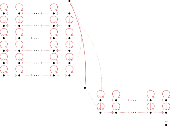
After these examples, one can derive the pattern in order to obtain an exponent of the form $p_0(k) + p_1(k)d_1^k + \cdots + p_n(k) d_n^k$ by simply adding more levels, i.e., by considering matrices of higher dimension, and gluing the corresponding graphs in an appropriate way. We write down the corresponding element that gives rise to such a pattern. If we let $N = m_0 + \cdots + m_n$ to be the sum of the degrees of the polynomials $p_0,\dots ,p_n$ respectively, with $p_i(x)=\sum _{j=0}^{m_i} a_{j,i}x^j$ for $0 \le i \le n$, then the element realizing the preceding pattern belongs to $M_{3N+n+5}({\mathcal {A}}_{1/2})$, and is given explicitly by

The elements in between connect the different polynomials $p_i$, and the contributions (monomials) of the polynomials (that is, the sum $p_0(k) + p_1(k)d_1^k + \cdots + p_n(k)d_n^k$) are accumulated in the $\chi _{[{\underline{0}}1]} \cdot e_{0,0}$ component. A simplified schematic of a prototypical graph appearing here is as follows.

Using the same procedure as before, a straightforward (but quite tedious) computation allows us to conclude the proof. We only write down the contribution corresponding to the components $C_4$ of the graph $E_A(W)$ where W is of the second type, which are the ones that contribute to the irrationality of the $\ell ^2$-Betti number. We get

$$\begin{aligned} \text {dim}_{{\mathbb Q}}(\ker \, A_{C_4}) = 2 + \delta _{k_{i+1},p_0(k_i) - k_i - a_{0,0} + p_1(k_i)d_1^{k_i} + \cdots + p_n(k_i)d_n^{k_i}}. \end{aligned}$$

We have $r-1$ connected components of this kind. Thus, the contribution to $b^{(2)}(A)$ coming from these graphs is

$$\begin{aligned}&\sum _{r \ge 1} \sum _{k_1,\dots ,k_r \ge 1} \frac{1}{2^{k_1 + \cdots + k_r + (r+3)}}\Big [ 2(r-1) + \sum _{i=1}^{r-1} \delta _{k_{i+1},p_0(k_i) - k_i - a_{0,0} + p_1(k_i)d_1^{k_i} + \cdots + p_n(k_i)d_n^{k_i}} \Big ] \\&\quad = \frac{2}{8} \sum _{r \ge 1}\frac{r-1}{2^r} + \frac{2^{a_{0,0}}}{8}\Big ( \sum _{r \ge 1} \frac{r-1}{2^r} \Big ) \Big ( \sum _{k \ge 1} \frac{1}{2^{p_0(k) + p_1(k)d_1^{k} + \cdots + p_n(k)d_n^{k}}} \Big ) \\&\quad = \frac{1}{4} + \frac{2^{a_{0,0}}}{8} \sum _{k \ge 1} \frac{1}{2^{p_0(k) + p_1(k)d_1^{k} + \cdots + p_n(k)d_n^{k}}}. \end{aligned}$$

We leave the rest of the details to the reader. Note, again, that in the special case $a_{0,0} = 0$ the irrational number $\alpha = \sum _{k \ge 1} \frac{1}{2^{p_0(k) + p_1(k)d_1^{k} + \cdots + p_n(k)d_n^{k}}}$ is accompanied by a rational number of the form $\frac{1}{2^m}$.

For the second part of the theorem, note that under the assumption $a_{0,0} = 0$ we have always obtained irrational numbers of the form $q_0 + q_1 \alpha$, being $\alpha$ the irrational number

$$\begin{aligned} \alpha = \sum _{k \ge 1} \frac{1}{2^{p_0(k) + p_1(k)d_1^{k} + \cdots + p_n(k)d_n^{k}}}, \end{aligned}$$

and $q_0,q_1$ nonzero rational numbers with $q_1$ of the form $\frac{1}{2^m}$ for some $m \ge 1$. In particular, $q_0 + q_1 \alpha$ belongs to ${\mathcal {G}}(\varGamma ,{\mathbb Q})$. By a result of Ara and Goodearl [4, Corollary 6.14], the group ${\mathcal {G}}(\varGamma ,{\mathbb Q})$ contains the rational numbers, and hence, the element $q_1 \alpha$ belongs to ${\mathcal {G}}(\varGamma ,{\mathbb Q})$ too. Since $q_1 = \frac{1}{2^m}$, we get

$$\begin{aligned} \alpha = q_1 \alpha + {\mathop {\cdots }\limits ^{2^m}} + q_1 \alpha \in {\mathcal {G}}(\varGamma ,{\mathbb Q}). \end{aligned}$$

This completes the proof of the theorem. $\square$

Remark 4.6

By making use of the ideas and techniques developed in Theorem 4.5, one can construct elements whose associated $\ell ^2$-Betti number has a binary expansion following different kinds of exotic patterns. For example, by gluing in an appropriate way two graphs corresponding to different polynomials $p_1(x)$ and $p_2(x)$, that is, by constructing graphs of the form $C_3$ but substituting the bottom right graph (the one contributing to $k_{i+1}$) by another graph corresponding to the polynomial $p_2(x)$, we can obtain terms in the computation of the associated $\ell ^2$-Betti number of the form

$$\begin{aligned} \sum _{k_1,k_2 \ge 1} \frac{\delta _{p_1(k_1),p_2(k_2)}}{2^{k_1+k_2}}, \end{aligned}$$

and more generally of the form

$$\begin{aligned} \sum _{k_1,k_2 \ge 1} \frac{\delta _{p_0(k_1) + p_1(k_1)d_1^{k_1} + \cdots + p_n(k_1) d_n^{k_1},q_0(k_2) + q_1(k_2)l_1^{k_2} + \cdots + q_m(k_2) l_m^{k_2}}}{2^{k_1+k_2}}, \end{aligned}$$

being $p_i(x),q_j(x)$ polynomials satisfying the hypotheses of the theorem, and $d_i,l_j \ge 2$ integers.

To conclude this section, it may be instructive to compute some rational values of $\ell ^2$-Betti numbers. In [19] (cf. [4, 13, 17]) the authors compute the $\ell ^2$-Betti number of the element $a_0 = e_0t + t^{-1} e_0 = \chi _{X \backslash E_0} t + t^{-1} \chi _{X \backslash E_0}$, which belongs to the first of our approximating algebras, ${\mathcal {A}}_0$. We will compute, in general, the $\ell ^2$-Betti number of the element $a_n = \chi _{X \backslash E_n} t + t^{-1} \chi _{X \backslash E_n} \in {\mathbb Q}\varGamma$ belonging to the $*$-subalgebra ${\mathcal {A}}_n$. Under $\pi _n$—and recalling that ${\mathfrak R}_n = {\mathbb Q}\times \prod _{k \ge 1} M_{m+k}({\mathbb Q})^{\text {Fib}_m(k)}$ with $m = 2n+1$—it gives

$$\begin{aligned} \pi _n(a_n) = ( 0, ( t_{m+k} + t_{m+k}^* , {\mathop {\dots }\limits ^{\text {Fib}_m(k)}}, t_{m+k} + t_{m+k}^*)_{k \ge 1}), \end{aligned}$$

where $t_r$ is the $r \times r$ lower triangular matrix given by

$$\begin{aligned} t_r = \left( \begin{array}{@{}c@{}} \begin{matrix} 0 &{}\quad &{}\quad &{}\quad &{}\quad \text{0 }\\ 1 &{}\quad 0 &{}\quad &{}\quad &{}\quad \\ &{} \quad \ddots &{}\quad \ddots &{}\quad &{}\quad \\ &{}\quad &{}\quad \ddots &{}\quad 0 &{}\quad \\ \text{0 }&{}\quad &{}\quad &{}\quad 1 &{}\quad 0 \end{matrix} \end{array} \right) . \end{aligned}$$

It is then straightforward to show that

$$\begin{aligned} \text {dim}_{{\mathbb Q}}(\ker \, (t_{m+k} + t_{m+k}^*)) = {\left\{ \begin{array}{ll} 1 &{} \text { if } k \text { is even} \\ 0 &{} \text { otherwise} \end{array}\right. } \end{aligned}$$

so

$$\begin{aligned} b^{(2)}(a_n) = \frac{1}{2^{m+1}} + \sum _{k \ge 1} \frac{\text {Fib}_m(2k)}{2^{2m+2k}}. \end{aligned}$$

This sum can be computed by using the summation rule

$$\begin{aligned} \sum _{k \ge 1} \frac{\text {Fib}_m(2k)}{2^{2k}} = 2^{m-1} \frac{2^{m+1}-1}{2^{m+2}+1}, \end{aligned}$$

whose proof can be found in [10, Lemma 3.2.11]. We then have

$$\begin{aligned} b^{(2)}(a_n) = \frac{3}{1+2^{2n+3}}. \end{aligned}$$

Note that $b^{(2)}(a_0) = \frac{1}{3}$, and we recover the result from [13, 19]. Also, as $n \rightarrow \infty$, this value tends to zero, as expected since $a_n \rightarrow t + t^{-1}$ in rank, which is invertible inside ${\mathfrak R}_{{\text {rk}}}$.

4.3 Rational series and $\ell ^2$-Betti numbers

In this section, we let again $K \subseteq {\mathbb C}$ be any field closed under complex conjugation. A more algebraic perspective to attack the problem of computing values from ${\mathcal {G}}({\mathcal {A}}_{1/2}) \subseteq {\mathcal {G}}(\varGamma ,K)$ is through the determination of the $*$-regular closure ${\mathcal {R}}_{1/2}$ of the algebra ${\mathcal {A}}_{1/2}$ seen inside ${\mathfrak R}_{1/2} = K \times \prod _{k \ge 1} M_{k+2}(K)^{\text {Fib}_2(k)}$ through the embedding $\pi _{1/2} : {\mathcal {A}}_{1/2} \hookrightarrow {\mathfrak R}_{1/2}$, and taking advantage of [3, Proposition 4.1] which states that the values of ranks of elements from ${\mathcal {R}}_{1/2}$ are all included in ${\mathcal {G}}(\varGamma ,K)$.

In order to clarify the exact relationship of this approach with Atiyah’s problem, it is convenient to introduce the following definitions for a general unital ring.

Definition 4.7

Let R be a unital ring and let ${\text {rk}}$ be a Sylvester matrix rank function on R. We denote by ${\mathcal {C}}_{{\text {rk}}} (R)$ the set of real numbers of the form $k- {\text {rk}}(A)$ for $A\in M_k(R)$, $k\ge 1$. We denote by ${\mathcal {C}}'_{{\text {rk}}}(R)$ the set of real numbers of the form ${\text {rk}}(A)$ for $A\in M_k(R)$, $k\ge 1$. Both ${\mathcal {C}}_{{\text {rk}}}(R)$ and ${\mathcal {C}}_{{\text {rk}}}'(R)$ are subsemigroups of $({\mathbb R}^+,+)$. We denote by ${\mathcal {G}}_{{\text {rk}}}(R)$ the subgroup of ${\mathbb R}$ generated by ${\mathcal {C}}_{{\text {rk}}}(R)$. Clearly

$$\begin{aligned} {\mathcal {G}}_{{\text {rk}}}(R)= {\mathcal {C}}_{{\text {rk}}}(R) - {\mathcal {C}}_{{\text {rk}}}(R) = {\mathcal {C}}_{{\text {rk}}}'(R) - {\mathcal {C}}_{{\text {rk}}}'(R). \end{aligned}$$

Remark 4.8

With this notation, [22, Corollary 6.2] says that, if ${\mathcal {U}}$ is a $*$-regular ring and R is a $*$-subring of ${\mathcal {U}}$ such that ${\mathcal {U}}$ is the $*$-regular closure of R in ${\mathcal {U}}$, then we have

$$\begin{aligned} {\mathcal {G}}_{{\text {rk}}} (R) = {\mathcal {G}}_{{\text {rk}}}({\mathcal {U}}) \end{aligned}$$

for every Sylvester matrix rank function ${\text {rk}}$ on ${\mathcal {U}}$. Thus, the main object of study within this approach is the group ${\mathcal {G}}_{{\text {rk}}}(R)$. Of course, ${\mathcal {C}}(G,K) = {\mathcal {C}}_{{\text {rk}}}(KG)$ for any discrete group G, where ${\text {rk}}$ is the canonical rank. It would be interesting to know conditions under which ${\mathcal {C}}_{{\text {rk}}}(R)= {\mathcal {C}}_{{\text {rk}}}'(R)$ and under which ${\mathcal {C}}_{{\text {rk}}}(R)= {\mathcal {G}}_{{\text {rk}}}(R)\cap {\mathbb R}^+$, or ${\mathcal {C}}_{{\text {rk}}}'(R)= {\mathcal {G}}_{{\text {rk}}}(R)\cap {\mathbb R}^+$. Note that

$$\begin{aligned} \forall g\in {\mathcal {G}}_{{\text {rk}}}(R)\, \exists t\in {\mathbb Z}^+ : g+t\in {\mathcal {C}}_{{\text {rk}}}(R) \iff \forall g\in {\mathcal {G}}_{{\text {rk}}}(R)\, \exists t\in {\mathbb Z}^+ : g+t\in {\mathcal {C}}_{{\text {rk}}}'(R). \end{aligned}$$

In case R is von Neumann regular, we have that ${\mathcal {C}}_{{\text {rk}}}(R) = {\mathcal {C}}_{{\text {rk}}}'(R)$ and the above equivalent conditions hold automatically, for every Sylvester matrix rank function ${\text {rk}}$.

We briefly remind some concepts from [3]. Write ${\mathcal {A}}_{1/2} = \bigoplus _{i\in {\mathbb Z}} {\mathcal {A}}_{1/2,i}t^i$, where ${\mathcal {A}}_{1/2,0}= {\mathcal {A}}_{1/2}\cap C_K(X)$ and

$$\begin{aligned} {\mathcal {A}}_{1/2,i}= & {} \chi _{X \setminus (E_{1/2} \cup T(E_{1/2}) \cup \cdots \cup T^{i-1}(E_{1/2}))} {\mathcal {A}}_{1/2,0} \quad \text {and} \\ {\mathcal {A}}_{1/2,-i}= & {} \chi _{X \setminus (T^{-1}(E_{1/2}) \cup \cdots \cup T^{-i}(E_{1/2}))} {\mathcal {A}}_{1/2,0} \end{aligned}$$

for $i > 0$. Following [3, Subsection 4.2], we consider a skew partial power series ring ${\mathcal {A}}_{1/2,0}[[t;T]]$ by taking infinite formal sums

$$\begin{aligned} \sum _{i \ge 0} b_i (\chi _{X \backslash E_{1/2}} t)^i = \sum _{i \ge 0} b_i t^i , \text { where } b_i \in {\mathcal {A}}_{1/2,i} \text { for all } i \ge 0. \end{aligned}$$

Specializing [3, Definition 4.17] to our situation, we see that a special term of positive degree i is a monomial $b_it^i$ in ${\mathcal {A}}_{1/2,i}$, where $b_i = \chi _S$ with

$$\begin{aligned} S = [10^{i_1}10^{i_2}1\cdots 10^{i_r}\underline{1}],\quad \text { where } r\ge 1, i_1,\dots ,i_r\ge 1 \text { and } i= i_1+\cdots +i_r +r. \end{aligned}$$

Moreover, since $E_{1/2}\cap T^{-1}(E_{1/2})\ne \emptyset$ and $S_0= T^{-1}(S_1)= [\underline{1}]$, we get from [3, Definition 4.7(c)] that the unique special term of degree 0 is $\chi _{[\underline{1}]}$.

Next, consider the subset ${\mathcal {S}}_{1/2}[[t;T]]$ of ${\mathcal {A}}_{1/2,0}[[t;T]]$ consisting of those elements

$$\begin{aligned} \sum _{i \ge 0} b_i (\chi _{X \backslash E_{1/2}}t)^i = \sum _{i \ge 0} b_i t^i \end{aligned}$$

such that each $b_it^i \in {\mathcal {A}}_{1/2,i}t^i$ belongs to the K-linear span of the special terms of degree i. We denote by ${\mathcal {S}}_{1/2} [t;T]$ the subspace of ${\mathcal {S}}_{1/2} [[t;T]]$ consisting of elements with finite support.

Let ${\mathscr {X}}=\{x_1,x_2,\dots \}$ be an infinite countable set, and consider the algebras $K\langle {\mathscr {X}}\rangle$ and $K\langle \langle {\mathscr {X}}\rangle \rangle$ of non-commutative polynomials and non-commutative formal power series, respectively, with coefficients in K. We consider the degree in $K\langle {\mathscr {X}}\rangle$ given by $d(x_i) = i+1$ for all $i\ge 1$ and $d(1)=0$. With this degree function, $K\langle {\mathscr {X}}\rangle$ is a graded K-algebra, where K has the trivial degree.

The following result is shown in [3, Lemma 6.5 and Proposition 6.6]. Note that [3, Propositions 6.6 and 6.7] are stated only for $n\ge 1$, but they hold, with the same proof, for $n=1/2$.

Proposition 4.9

The linear subspaces ${\mathcal {S}}_{1/2}[t;T]$ and ${\mathcal {S}}_{1/2}[[t;T]]$ are indeed subalgebras of ${\mathcal {A}}_{1/2}[[t;T]]$. There is an isomorphism of unital graded algebras $K\langle {\mathscr {X}}\rangle \cong {\mathcal {S}}_{1/2} [t; T]$ sending the element $x_{i_r}\cdots x_{i_1}$ to $\chi _{[10^{i_1}10^{i_2}1\cdots 10^{i_r}\underline{1}]}t^{i}$, where $i=i_1+\cdots + i_r+r$, and 1 to $\chi _{[\underline{1}]}$. This isomorphism extends naturally to an isomorphism between $K\langle \langle {\mathscr {X}}\rangle \rangle$ and ${\mathcal {S}}_{1/2}[[t;T]]$.

The special terms of the form $\chi _{[10^i\underline{1}]}t^{i+1}$, for $i\ge 1$, which are the algebra generators of ${\mathcal {S}}_{1/2}[t;T]$, are called pure special terms, see the proof of [3, Proposition 6.6].

Let ${\mathscr {X}}^*$ denote the free monoid on ${\mathscr {X}}$. We now recall the concept of the Hadamard product $\odot$ on $K\langle \langle {\mathscr {X}}\rangle \rangle$, see [9] for more details. If $a= \sum _{w\in {\mathscr {X}}^*}a_ww$ and $b= \sum _{w\in {\mathscr {X}}^*} b_ww$ are elements in $K\langle \langle {\mathscr {X}}\rangle \rangle$, set

$$\begin{aligned} a\odot b = \Big (\sum _{w\in {\mathscr {X}}^*}a_ww\Big )\odot \Big (\sum _{w\in {\mathscr {X}}^*} b_ww\Big ) = \sum _{w\in {\mathscr {X}}^*} (a_wb_w)w \in K\langle \langle {\mathscr {X}}\rangle \rangle . \end{aligned}$$

We will denote by $K\langle \langle {\mathscr {X}}\rangle \rangle ^{\circ }$ the algebra of non-commutative formal power series endowed with the Hadamard product. Note that $K\langle \langle {\mathscr {X}}\rangle \rangle ^{\circ }$ is a $*$-regular ring with respect to the involution given by $\overline{\sum _{w\in {\mathscr {X}}^*}a_ww}= \sum _{w\in {\mathscr {X}}^*} \overline{a_w}w$. The algebra of non-commutative rational series, denoted by $K_{\text {rat}}\langle {\mathscr {X}}\rangle$ is defined as the division closure of $K\langle {\mathscr {X}}\rangle$ in $K\langle \langle {\mathscr {X}}\rangle \rangle$, that is, $K_{\text {rat}}\langle {\mathscr {X}}\rangle$ is the smallest subalgebra of $K\langle \langle {\mathscr {X}}\rangle \rangle$ containing $K\langle {\mathscr {X}}\rangle$ and closed under inversion, see [9] for details. It is well known that $K_{\text {rat}}\langle {\mathscr {X}}\rangle$ is closed under the Hadamard product [9, Theorems 1.5.5 and 1.7.1].

Let $p_{1/2} :=p_{E_{1/2}}= \pi _{1/2}(\chi _{E_{1/2}})$ be the projection in ${\mathfrak R}_{1/2}= \prod _{W\in \mathbb {V}_{1/2}} M_{|W|}(K) = K\times \prod _{k \ge 1} M_{k+2}(K)^{\text {Fib}_2(k)}$ which has a 1 in the left upper corner of each matrix factor $M_{|W|}(K)$, and $0's$ elsewhere, that is, $(p_{1/2})_W= e_{00}(W)$ for each $W\in \mathbb {V}_{1/2}$. Recall from the beginning of Sect. 4.2 that the elements of $\mathbb {V}_{1/2}$ are all the clopen sets of the form $[1\underline{1}0^{i_1}10^{i_2}1\cdots 10^{i_r}11]$, where $r\ge 0$ and $i_1,\dots i_r\ge 1$. (We interpret this term to be $[1\underline{1}1]$ if $r=0$.)

By [3, Proposition 4.20], there is a $*$-isomorphism from $({\mathcal {S}}_{1/2}[[t;T]],\odot ,-)$ onto $p_{1/2}{\mathfrak R}_{1/2} p_{1/2}$. Composing the isomorphism $K\langle \langle {\mathscr {X}}\rangle \rangle \cong {\mathcal {S}}_{1/2} [[t;T]]$ from Proposition 4.9 (which respects the respective Hadamard products and involutions) with this isomorphism, we obtain a $*$-isomorphism

$$\begin{aligned} \Delta :K\langle \langle {\mathscr {X}}\rangle \rangle ^{\circ } \overset{\cong }{\longrightarrow } p_{1/2}{\mathfrak R}_{1/2} p_{1/2} \end{aligned}$$

such that

$$\begin{aligned} \Delta (f)_{[1\underline{1}0^{i_1}1\cdots 10^{i_r}11]} = (f, x_{i_r}\cdots x_{i_1})e_{00}([1\underline{1}0^{i_1}1\cdots 10^{i_r}11]) \qquad (f\in K\langle \langle {\mathscr {X}}\rangle \rangle ) \end{aligned}$$

for each $i_1,\dots ,i_r\ge 1$. Here, $(f, x_{i_r}\cdots x_{i_1})$ is the coefficient of f corresponding to the monomial $x_{i_r}\cdots x_{i_1}$.

For each $n\ge 1$, set ${\mathscr {X}}_n=\{ x_1,\dots , x_n\}$. Let L be a language over ${\mathscr {X}}_n$, i.e., a subset of the free monoid ${\mathscr {X}}_n^*$ on ${\mathscr {X}}_n$. We now give a formula for the rank of the element $\Delta (\underline{L})$, where

$$\begin{aligned} \underline{L} := \sum _{w\in L} w \in K\langle \langle {\mathscr {X}}_n \rangle \rangle \end{aligned}$$

is the characteristic series of L ( [9, p.8]). Note that, for $W=[1\underline{1}0^{i_1}10^{i_2}1\cdots 10^{i_r}11]\in \mathbb {V}_{1/2}$, we have

$$\begin{aligned} \Delta (\underline{L})_W= {\left\{ \begin{array}{ll} e_{00}(W) &{} \text { if } x_{i_r}\cdots x_{i_2}x_{i_1}\in L \\ 0 &{} \text { if } x_{i_r}\cdots x_{i_2}x_{i_1}\notin L\end{array}\right. }. \end{aligned}$$

Moreover, we have $\mu (W)= 2^{-(i_1+\cdots +i_r+r+3)}= 2^{-3}2^{-d(w)}$, where $w=x_{i_r}\cdots x_{i_2}x_{i_1}$. Let $s(L)= \sum _{j\ge 0} \alpha _j x^j$ be the series in ${\mathbb Z}^+[[x]]$ such that $\alpha _j$ is the number of words $w\in L$ such that $d(w)= j$. Then we have

$$\begin{aligned} {\text {rk}}(\Delta (\underline{L})) = \sum _{W \in {\mathbb V}_{1/2}} \mu (W) {\text {Rk}}(\Delta (\underline{L})_W) = \frac{1}{2^3}\sum _{w\in L} \frac{1}{2^{d(w)}} = \frac{1}{8}s(L)\Big (\frac{1}{2}\Big ). \end{aligned}$$

(4.3)

Here we make use of (3.2) for the first equality, of the above observations for the second, and of the definition of s(L) for the third. We say that $s(L) \in {\mathbb Z}^+[[x]]$ is the generating function of L with respect to d, and we denote by $\alpha _L$ the real number ${\text {rk}}(\Delta (\underline{L}))$ described in (4.3).

We now recall the notion of a rational language (see [9, Chapter 3]).

Definition 4.10

The set of rational languages over a finite set F is the smallest set of subsets of the free monoid $F^*$ containing all the finite subsets of $F^*$ and closed under the following operations:

• (a) union $L_1\cup L_2$;

• (b) product $L_1L_2 := \{w_1 w_2 \in F^* \mid w_1 \in L_1, w_2 \in L_2\}$;

• (c) $*$-product $L^* := \bigcup _{k \ge 0} L^k$.

A characterization of the rational languages is the following ([9, Lemma 3.1.4]): a language over a finite alphabet F is rational if and only if it is the support of some rational series $z \in {\mathbb Z}^+ \langle \langle F \rangle \rangle$. In fact, if L is a rational language over F, its characteristic series $\underline{L} = \sum _{w \in L}w$ belongs to $R_{\mathrm {rat}}\langle F \rangle ^{\circ }$ for any semiring R ([9, Proposition 3.2.1]).

It turns out that the set of rational languages over F, which we will denote by ${\mathfrak L}(F)$, forms a Boolean subalgebra of $P (F^*)$, the power set of $F^*$ ([9, Corollary 3.1.5]). However, the converse may not be true. Indeed, for a subfield K of ${\mathbb C}$ closed under complex conjugation, given a rational series $z = \sum _{w \in F^*} \lambda _w w \in K_{\mathrm {rat}}\langle F \rangle$ it may be the case that its support $L = \text {supp}(z)$ is not a rational language. We put

$$\begin{aligned} \mathfrak K(F) := \{ \text {supp}(z) \mid z \in K_{\mathrm {rat}}\langle F \rangle ^{\circ }\} \subseteq P(F^*), \end{aligned}$$

and we let $\mathbf{B }_{\text {rat}}^K(F)$ be the Boolean algebra of subsets of $F^*$ generated by $\mathfrak K (F)$. Then by [3, Proposition 6.10] the $*$-regular closure of $K_{\text {rat}}\langle F\rangle ^{\circ }$ in $K\langle \langle F\rangle \rangle ^{\circ }$ is contained in the set of formal power series whose support belongs to $\mathbf{B }_{\mathrm {rat}}^K(F)$, and for each set $L\in \mathbf{B }_{\mathrm {rat}}^K(F)$, the characteristic series $\underline{L}$ belongs to the $*$-regular closure.

We gather some of these facts in the following.

Proposition 4.11

Let $n\ge 1$ and let ${\mathscr {X}}_n=\{x_1,\dots , x_n\}$, endowed with the degree function $d(x_i)= i+1$. With the above notation, we have ${\mathfrak L}({\mathscr {X}}_n) \subseteq \mathfrak K ({\mathscr {X}}_n) \subseteq {\varvec{{B}}}_{\mathrm {rat}}^K({\mathscr {X}}_n)$. The sets ${\mathfrak L}({\mathscr {X}}_n)$ and ${\varvec{{B}}}_{\mathrm {rat}}^K({\mathscr {X}}_n)$ are Boolean subalgebras of $P({\mathscr {X}}_n^*)$, but this is not the case in general for $\mathfrak K ({\mathscr {X}}_n)$. Moreover, if $L\in \mathbf{B }_{\mathrm {rat}}^K({\mathscr {X}}_n)$, then $\alpha _L\in {\mathcal {G}}(\varGamma , K)$.

Proof

See [9, Chapter 3]. The fact that $\alpha _L\in {\mathcal {G}}(\varGamma , K)$ for $L\in \mathbf{B }_{\mathrm {rat}}^K({\mathscr {X}}_n)$ follows from [3, Propositions 4.1, 4.26, 6.7 and 6.10]. $\square$

We now show that rational languages give rise to rational $\ell ^2$-Betti numbers.

Lemma 4.12

If a series $\sum _{j \ge 0} \alpha _j x^j \in {\mathbb Z}^+[[x]]$ is the generating function of a rational language $L \in {\mathfrak L}({\mathscr {X}}_n)$ with respect to d, then it is a rational series with constant term either 0 or 1. Consequently, $\alpha _L \in {\mathbb Q}$.

Proof

Suppose $\alpha _j = \#(L \cap d^{-1}(\{j\}))$, being $L \in {\mathfrak L}({\mathscr {X}}_n)$ a rational language. In particular the series $\underline{L}= \sum _{w \in L}w$ is rational. Define a map $\rho : {\mathscr {X}}_n \rightarrow {\mathbb Z}^+[[x]]$ by setting $\rho (b) = x^{d(b)}$. By [9, Proposition 1.4.2], the map $\rho$ extends uniquely to a morphism $\rho : {\mathbb Z}^+\langle \langle {\mathscr {X}}_n \rangle \rangle \rightarrow {\mathbb Z}^+[[x]]$ which induces the identity on ${\mathbb Z}^+$ and, moreover, preserves rationality. Then

$$\begin{aligned} \rho \Big ( \sum _{w \in L}w \Big ) = \sum _{w \in L}x^{d(w)} = \sum _{j \ge 0} \alpha _j x^j \end{aligned}$$

is rational in ${\mathbb Z}^+[[x]]$, and clearly its constant term is either 0 or 1.

By [9, Proposition 6.1.1], there exist polynomials $p(x),q(x) \in {\mathbb Z}[x]$ such that the series $\sum _{j \ge 0}\alpha _j x^j$ is the power series expansion of the rational function $\frac{p(x)}{1-xq(x)}$, that is,

$$\begin{aligned} s(L) = \sum _{j \ge 0}\alpha _j x^j = \frac{p(x)}{1-xq(x)} = p(x) \Big [1 + \sum _{j \ge 0}(xq(x))^j\Big ]. \end{aligned}$$

Consequently, if $L \in {\mathfrak L}({\mathscr {X}}_n)$, then $\alpha _L = \frac{1}{8}s(L)\big (\frac{1}{2}\big ) \in {\mathbb Q}$. $\square$

We obtain now a concrete irrational algebraic number of the form $\alpha _L$ for a suitable $L\in \mathbf{B }_{\text {rat}}^{{\mathbb Q}}({\mathscr {X}}_2)$.

Theorem 4.13

There is $L\in \mathbf{B }_{\mathrm{rat}}^{{\mathbb Q}}({\mathscr {X}}_2)$ such that $\alpha _L=\frac{1}{4}\sqrt{\frac{2}{7}}$. In particular, $\frac{1}{4}\sqrt{\frac{2}{7}}\in {\mathcal {G}}(\varGamma , \mathbb {Q})$.

Proof

Let L be the language on ${\mathscr {X}}_2=\{x_1,x_2\}$ given by

$$\begin{aligned} L= \{ w\in {\mathscr {X}}_2^* \mid |w|_{x_1} =|w|_{x_2} \}. \end{aligned}$$

Here $|w|_{x_i}$ is the number of appearances of $x_i$ in w, for $i=1,2$. Then by [9, Example 3.4.1], $L\in \mathbf{B }_{\text {rat}}^{{\mathbb Q}}({\mathscr {X}}_2)$ (although L is not a rational language). If $w\in L$, then since $d(x_1)= 2$ and $d(x_2)=3$, we get that $d(w)=5l$, where $l=|w|_{x_1}=|w|_{x_2}$. Therefore, we get from Proposition 4.11 that

$$\begin{aligned} \alpha _L = \frac{1}{8} \sum _{j \ge 0} \frac{\alpha _j}{2^j} = \frac{1}{8} \sum _{l\ge 0} \left( {\begin{array}{c}2l\\ l\end{array}}\right) \frac{1}{2^{5l}} \in {\mathcal {G}}(\varGamma , {\mathbb Q}). \end{aligned}$$

Since

$$\begin{aligned} \sum _{l\ge 0} \left( {\begin{array}{c}2l\\ l\end{array}}\right) x^l = \frac{1}{\sqrt{1-4x}} \quad \text { for } |x| < \frac{1}{4}, \end{aligned}$$

we obtain $\alpha _L = \frac{1}{4}\sqrt{\frac{2}{7}} \in {\mathcal {G}}(\varGamma , {\mathbb Q})$. $\square$

Taking different choices of variables $x_r,x_s$, with $r\ne s$, we indeed obtain that ${\mathcal {G}}(\varGamma , {\mathbb Q})$ contains all the algebraic numbers

$$\begin{aligned} \frac{1}{8}\sqrt{\frac{2^t}{2^t-1}}, \quad \text { for } t \ge 3. \end{aligned}$$

Similar formulas can be obtained to compute the ranks of elements coming from the copy of the algebra ${\mathbb Q}_{\text {rat}}\langle {\mathscr {X}}\rangle$ in the $*$-regular closure ${\mathcal {R}}_n$ of ${\mathcal {A}}_n$ in $\mathfrak R_n$, where ${\mathcal {A}}_n$ are the approximations of ${\mathbb Q}\varGamma$ described in Sect. 4.1. The only differences are that we have different degree functions on ${\mathscr {X}}$, depending on n, and that the factor 1/8 must be substituted by the factor $2^{-2n-2}$.

Remark 4.14

By Theorem 4.13, $\frac{1}{4}\sqrt{\frac{2}{7}}$ is a ‘virtual’ $\ell ^2$-Betti number arising from the lamplighter group $\varGamma$. This means that there are two $\ell ^2$-Betti numbers arising from $\varGamma$, $\alpha _1$ and $\alpha _2$, such that $\frac{1}{4}\sqrt{\frac{2}{7}} = \alpha _1 - \alpha _2$. It would be interesting to know whether $\frac{1}{4}\sqrt{\frac{2}{7}}$ is itself an $\ell ^2$-Betti number, and in that case, to determine a concrete matrix over $\mathbb {Q} \varGamma$ witnessing this fact. In particular, this would solve a question posed by Grabowski in [17, p. 32], see also [18, Question 3]. We do not know any example of a group G for which ${\mathcal {C}}(G,\mathbb {Q}) \ne {\mathcal {G}}(G,\mathbb {Q})\cap \mathbb {R}^+$.

We close this section with the following problem:

Question 4.15

With the notation established before, is $\alpha _L$ always an algebraic number when $L \in \mathbf{B }_{\mathrm{rat}}^{{\mathbb Q}}({\mathscr {X}}_n)$?

5 The odometer algebra

In this last section, we focus on computing the whole set of values that the Sylvester matrix rank function constructed from Theorem 3.2 can achieve in the case of the generalized odometer algebra. We first recall its definition.

Fix a sequence of natural numbers $\overline{n} = (n_i)_{i \in {\mathbb N}}$ with $n_i \ge 2$ for all $i \in {\mathbb N}$, and consider $X_i$ to be the finite space $\{0,1,\dots ,n_i-1\}$ endowed with the discrete topology. From these we form the topological space $X = \prod _{i \in {\mathbb N}}X_i$ endowed with the product topology, which is in fact a Cantor space. Let T be the homeomorphism on X given by the odometer, namely for $x = (x_i) \in X$, T is given by

$$\begin{aligned} T(x) = {\left\{ \begin{array}{ll} (x_1+1,x_2,x_3,\dots ) &{} \text { if } x_1 \ne n_1-1, \\ (0,\dots ,0,x_{m+1} + 1,x_{m+2},\dots ) &{} \text { if } x_j = n_j-1 \text { for } 1 \le j \le m \text { and } x_{m+1} \ne n_m-1, \\ (0,0,\dots ) &{} \text { if } x_i = n_i-1 \text { for all }i \in {\mathbb N}. \end{array}\right. } \end{aligned}$$

Note that the odometer action is just addition of $(1,0,\dots )$ by carryover.

Let $(K,-)$ be any field with a positive definite involution −. The generalized odometer algebra is defined as the crossed product $*$-algebra ${\mathcal {O}}(\overline{n}) := C_K(X) \rtimes _T {\mathbb Z}$. We obtain a measure $\mu$ on X by taking the usual product measure, where we consider the measure on each component $X_i$ which assigns mass $\frac{1}{n_i}$ on each point in $X_i$. It is well known (e.g., [11, Section VIII.4]) that $\mu$ is an ergodic, full and T-invariant probability measure on X, which in turn coincides with the Haar measure $\widehat{\mu }$ on X if one considers X as an abelian group with addition by carryover. We denote by ${\text {rk}}_{{\mathcal {O}}(\overline{n})}$ the Sylvester matrix rank function on ${\mathcal {O}}(\overline{n})$ given by Theorem 3.2.

5.1 Characterizing the $*$-regular closure ${\mathcal {R}}_{{\mathcal {O}}(\overline{n})}$

We explicitly compute the $*$-regular closure ${\mathcal {R}}_{{\mathcal {O}}(\overline{n})}$ of the odometer algebra. Recall that it is defined as the $*$-regular closure of ${\mathcal {O}}(\overline{n})$ inside ${\mathfrak R}_{{\text {rk}}}$ through the embedding ${\mathcal {O}}(\overline{n}) \hookrightarrow {\mathfrak R}_{{\text {rk}}}$ given by Theorem 3.2. We will use the notation $[a_1a_2 \dots a_r]$ for the cylinder sets $\{ (x_j)_{j\in {\mathbb N}}\mid x_i=a_i, 1 \le i \le r\}$, where $0\le a_i < n_i$, $1 \le i \le r$.

Define new integers $p_m := n_1 \cdots n_m$ for $m \in {\mathbb N}$. At each level $m \ge 1$, we take $E_m = [0 0 \cdots 0]$ (with m zeroes) for the sequence of clopen sets, whose intersection gives the point $y = (0,0,\dots ) \in X$. We take the partition ${\mathcal {P}}_m$ of the complement $X \backslash E_m$ to be the obvious one, namely

$$\begin{aligned} {\mathcal {P}}_m = \{[{1} 0 \cdots 0], \dots , [{(n_1-1)} 0 \cdots 0],\dots , [{(n_1-1)} (n_2-1) \cdots (n_m-1)]\}. \end{aligned}$$

We denote by ${\mathcal {O}}(\overline{n})_m$ the unital $*$-subalgebra of ${\mathcal {O}}(\overline{n})$ generated by the partial isometries $\{\chi _Z t \mid Z \in {\mathcal {P}}_m\}$. The quasi-partition $\overline{{\mathcal {P}}}_m$ is really simple in this case: write $Z_{m,l} = T^l(E_m)$ for $1 \le l < p_m$. Note that these clopen sets form exactly the partition ${\mathcal {P}}_m$, and that $T(Z_{m,p_m-1}) = E_m$. Therefore, there is only one possible $W \in {\mathbb V}_m$, which has length $p_m$ and is given by

$$\begin{aligned} W = E_m \cap T^{-1}(Z_{m,1}) \cap T^{-2}(Z_{m,2}) \cap \cdots \cap T^{-p_m+1}(Z_{m,p_m-1}) \cap T^{-p_m}(E_m) = E_m. \end{aligned}$$

The representations $\pi _m : {\mathcal {O}}(\overline{n})_m \rightarrow {\mathfrak R}_m, x \mapsto (h_W \cdot x)_W$ become $*$-isomorphisms, where ${\mathfrak R}_m = M_{p_m}(K)$. Under this identification, the embeddings $\iota _m : {\mathcal {O}}(\overline{n})_m \hookrightarrow {\mathcal {O}}(\overline{n})_{m+1}$ become the block-diagonal embeddings

$$\begin{aligned} M_{p_m}(K) \hookrightarrow M_{p_{m+1}}(K), \quad x \mapsto \text {diag}(x,{\mathop {\dots }\limits ^{n_{m+1}}},x), \end{aligned}$$

so that ${\mathcal {O}}(\overline{n})_{\infty } := \varinjlim _m {\mathcal {O}}(\overline{n})_m \cong \varinjlim _m M_{p_m}(K)$. Note that ${\mathcal {O}}(\overline{n})_{\infty }$ is already $*$-regular, but it does not contain ${\mathcal {O}}(\overline{n})$: in fact, it is contained in ${\mathcal {O}}(\overline{n})$. Intuitively, in order to get containment of the whole algebra ${\mathcal {O}}(\overline{n})$ we need to adjoin to ${\mathcal {O}}(\overline{n})_{\infty }$ the element t.

Definition 5.1

For every $m \ge 1$, we denote by ${\mathcal {O}}(\overline{n})^t_m$ the unital $*$-subalgebra of ${\mathcal {O}}(\overline{n})$ generated by ${\mathcal {O}}(\overline{n})_m$ and t.

We can completely characterize these $*$-subalgebras.

Lemma 5.2

There exists a $*$-isomorphism ${\mathcal {O}}(\overline{n})^t_m \cong M_{p_m}(K[t^{p_m}, t^{-p_m}])$.

Proof

For $0 \le i,j < p_m$, the elements $e_{ij}^{(m)} := e_{ij}(E_m)$ form a complete system of matrix units inside ${\mathcal {O}}(\overline{n})^t_m$, so there is an isomorphism ${\mathcal {O}}(\overline{n})^t_m \cong M_{p_m}(T)$ with T being the centralizer of the family $\{e_{ij}^{(m)} \mid 0 \le i,j < p_m\}$ in ${\mathcal {O}}(\overline{n})^t_m$. The isomorphism is given explicitly by

$$\begin{aligned} a \mapsto \sum _{i,j=0}^{p_m-1} a_{ij} e_{ij}^{(m)}, \quad \text { with } a_{ij} = \sum _{k=0}^{p_m-1} e_{ki}^{(m)} \cdot a \cdot e_{jk}^{(m)} \in T, \end{aligned}$$

which is also a $*$-isomorphism. Since $t^{p_m} e_{ij}^{(m)} t^{-p_m} = e_{ij}^{(m)}$ and

$$\begin{aligned} t = \sum _{i=0}^{p_m-1} t e_{ii}^{(m)} = \sum _{i=0}^{p_m-2} e_{i+1,i}^{(m)} + t^{p_m} e_{0,p_m-1}^{(m)} \in M_{p_m}(K[t^{p_m},t^{-p_m}]), \end{aligned}$$

we deduce that $T = K[t^{p_m},t^{-p_m}]$, as desired. $\square$

The inclusion ${\mathcal {O}}(\overline{n})^t_m \subseteq {\mathcal {O}}(\overline{n})^t_{m+1}$ translates to an embedding from $M_{p_m}(K[t^{p_m},t^{-p_m}])$ to $M_{p_{m+1}}(K[t^{p_{m+1}},t^{-p_{m+1}}])$ that extends the previous one $M_{p_m}(K) \hookrightarrow M_{p_{m+1}}(K)$, and sends the element $t^{p_m} \cdot \text {Id}_{p^m}$ to the element

Lemma 5.3

${\mathcal {O}}(\overline{n})$ is $*$-isomorphic to the direct limit $\varinjlim _m M_{p_m}(K[t^{p_m},t^{-p_m}])$ with respect to the previous embeddings.

Proof

By Remark 3.1, the algebra ${\mathcal {O}}(\overline{n})_{\infty }$ contains $C_K(X)$; hence, the $*$-subalgebra of ${\mathcal {O}}(\overline{n})$ generated by t and ${\mathcal {O}}(\overline{n})_{\infty }$ is ${\mathcal {O}}(\overline{n})$ itself. Now each ${\mathcal {O}}(\overline{n})_m$ sits inside ${\mathcal {O}}(\overline{n})^t_m$; hence, ${\mathcal {O}}(\overline{n})_{\infty } = \varinjlim _m {\mathcal {O}}(\overline{n})_m \subseteq \varinjlim _m {\mathcal {O}}(\overline{n})^t_m$. But $t \in \varinjlim _m {\mathcal {O}}(\overline{n})^t_m$ already, so ${\mathcal {O}}(\overline{n}) = \varinjlim _m {\mathcal {O}}(\overline{n})^t_m \cong \varinjlim _m M_{p_m}(K[t^{p_m},t^{-p_m}])$ by Lemma 5.2. $\square$

We are now ready to compute ${\mathcal {R}}_{{\mathcal {O}}(\overline{n})}$.

Theorem 5.4

There is a $*$-isomorphism ${\mathcal {R}}_{{\mathcal {O}}(\overline{n})} \cong \varinjlim _m M_{p_m}(K(t^{p_m}))$, where the maps $M_{p_m}(K(t^{p_m})) \hookrightarrow M_{p_{m+1}}(K(t^{p_{m+1}}))$ are induced by the inclusions of matrices over Laurent polynomial rings.

Proof

We have embeddings ${\mathcal {O}}(\overline{n})^t_m \hookrightarrow {\mathcal {O}}(\overline{n}) \hookrightarrow {\mathcal {R}}_{{\mathcal {O}}(\overline{n})} \hookrightarrow {\mathfrak R}_{{\text {rk}}}$. By [3, Lemma 4.4], the rational function field $K(t^{p_m})$ sits inside ${\mathcal {R}}_{{\mathcal {O}}(\overline{n})}$. Hence, there is, for each $m \ge 1$, a commutative diagram

It is straightforward to prove that for any nonzero element $q(t) \in K[t^{p_m},t^{-p_m}]$, the corresponding matrix in $M_{p_{m+1}}(K[t^{p_{m+1}}, t^{-p_{m+1}}])$ becomes invertible in $M_{p_{m+1}}(K(t^{p_{m+1}}))$. Therefore, the embedding ${\mathcal {O}}(\overline{n})^t_m \hookrightarrow {\mathcal {O}}(\overline{n})^t_{m+1}$ extends uniquely to an embedding $M_{p_m}(K(t^{p_m})) \hookrightarrow M_{p_{m+1}}(K(t^{p_{m+1}}))$, and the previous commutative diagrams give embeddings

$$\begin{aligned} {\mathcal {O}}(\overline{n}) \cong \varinjlim _m {\mathcal {O}}(\overline{n})^t_m \hookrightarrow \varinjlim _m M_{p_m}(K(t^{p_m})) \hookrightarrow {\mathcal {R}}_{{\mathcal {O}}(\overline{n})}. \end{aligned}$$

But $\varinjlim _m M_{p_m}(K(t^{p_m}))$ is already $*$-regular and contains ${\mathcal {O}}(\overline{n})$, so necessarily ${\mathcal {R}}_{{\mathcal {O}}(\overline{n})} \cong \varinjlim _m M_{p_m}(K(t^{p_m}))$, as required. $\square$

In particular, since $\varinjlim _m M_{p_m}(K(t^{p_m}))$ has a unique Sylvester matrix rank function, it coincides with the one given by Theorem 3.2 under the previous $*$-isomorphism.

5.2 Characterizing the set ${\mathcal {C}}'({\mathcal {O}}(\overline{n}))$

We characterize the set ${\mathcal {C}}'({\mathcal {O}}(\overline{n}))$ of all positive real values that the Sylvester matrix rank function ${\text {rk}}_{{\mathcal {O}}(\overline{n})}$ can achieve, and the subgroup ${\mathcal {G}}({\mathcal {O}}(\overline{n}))$ it generates. First, let

$$\begin{aligned} {\mathcal {C}}'({\mathcal {R}}_{{\mathcal {O}}(\overline{n})}) := {\text {rk}}_{{\mathcal {R}}_{{\mathcal {O}}(\overline{n})}}\Big ( \bigcup _{k \ge 1} M_k({\mathcal {R}}_{{\mathcal {O}}(\overline{n})}) \Big ) \subseteq {\mathbb R}^+ \end{aligned}$$

and note that ${\mathcal {C}}'({\mathcal {O}}(\overline{n})) \subseteq {\mathcal {C}}'({\mathcal {R}}_{{\mathcal {O}}(\overline{n})})= {\mathcal {C}}({\mathcal {R}}_{{\mathcal {O}}(\overline{n})})$ (see Definition 4.7 and Remark 4.8). The following definition will be essential.

Definition 5.5

For each sequence $\overline{n} = (n_1,n_2,\dots )$ of positive integers $n_i \ge 2$, one may associate with it the supernatural number

$$\begin{aligned} n = \prod _{i \in {\mathbb N}} n_i = \prod _{q \in \P }q^{\varepsilon _q(n)}, \end{aligned}$$

where $\P$ is the set of prime numbers ordered with respect to the natural ordering, and each $\varepsilon _q(n) \in \{0\} \cup {\mathbb N}\cup \{\infty \}$. In more detail, if $n_i = \prod _{q \in \P }q^{\varepsilon _q(n_i)}$ is the prime decomposition of $n_i$, then, for each $q\in \P$, $\varepsilon _q (n)$ is defined by $\varepsilon _q (n) = \sum _{i=1}^{\infty } \varepsilon _q (n_i) \in \{0\} \cup {\mathbb N}\cup \{\infty \}$, and n is defined as the formal product $\prod _{q \in \P }q^{\varepsilon _q(n)}$.

As in [26, Definition 7.4.2], from any supernatural number n one can construct an additive subgroup of ${\mathbb Q}$ containing 1, denoted by ${\mathbb Z}(n)$, consisting of those fractions $\frac{a}{b}$ with $a \in {\mathbb Z}$, and $b \in {\mathbb Z}\backslash \{0\}$ being of the form

$$\begin{aligned} b = \prod _{q \in \P } q^{\varepsilon _q(b)}, \end{aligned}$$

where $\varepsilon _q(b) \le \varepsilon _q(n)$ for all $q \in \P$, and $\varepsilon _q(b) = 0$ for all but finitely many q’s. If n comes from a sequence $\overline{n} = (n_1,n_2,\dots )$ as above, ${\mathbb Z}(n)$ is exactly the additive subgroup of ${\mathbb Q}$ consisting of those fractions of the form

$$\begin{aligned} \frac{a}{n_1 \cdots n_r}, \quad \text { with } a \in {\mathbb Z}\text { and } r \ge 1. \end{aligned}$$

Each group ${\mathbb Z}(n)$ gives rise to a subgroup $\mathbb {G} (n)={\mathbb Z}(n)/{\mathbb Z}$ of the group ${\mathbb Q}/{\mathbb Z}$. Indeed the groups $\mathbb {G} (n)$ describe all the subgroups of ${\mathbb Q}/{\mathbb Z}$. These groups are called Prüfer groups.

Theorem 5.6

We have ${\mathcal {C}}'({\mathcal {O}}(\overline{n})) = {\mathcal {C}}({\mathcal {O}}(\overline{n})) = {\mathcal {C}}'({\mathcal {R}}_{{\mathcal {O}}(\overline{n})}) = {\mathbb Z}(n)^+$. In particular, ${\mathcal {G}}({\mathcal {O}}(\overline{n})) = {\mathbb Z}(n)$.

Proof

The argument is similar to the one given in the proof of [3, Proposition 4.1]. Since ${\mathcal {R}}_{{\mathcal {O}}(\overline{n})}$ is a $*$-regular ring with positive definite involution, each matrix algebra $M_k({\mathcal {R}}_{{\mathcal {O}}(\overline{n})})$ is also $*$-regular. Hence, for each $A \in M_k({\mathcal {R}}_{{\mathcal {O}}(\overline{n})})$ there exists a projection $P \in M_k({\mathcal {R}}_{{\mathcal {O}}(\overline{n})})$ such that ${\text {rk}}_{{\mathcal {R}}_{{\mathcal {O}}(\overline{n})}}(A) = {\text {rk}}_{{\mathcal {R}}_{{\mathcal {O}}(\overline{n})}}(P)$. We conclude that ${\mathcal {C}}'({\mathcal {R}}_{{\mathcal {O}}(\overline{n})})$ equals the set of positive real numbers of the form ${\text {rk}}_{{\mathcal {R}}_{{\mathcal {O}}(\overline{n})}}(P)$, where P ranges over matrix projections with coefficients in ${\mathcal {R}}_{{\mathcal {O}}(\overline{n})}$. Now each such projection P is equivalent to a diagonal projection [16, Proposition 2.10], that is of the form $\text {diag}(p_1,p_2,\dots ,p_r)$ for some projections $p_1,\dots ,p_r \in {\mathcal {R}}_{{\mathcal {O}}(\overline{n})}$, so that ${\text {rk}}_{{\mathcal {R}}_{{\mathcal {O}}(\overline{n})}}(P) = {\text {rk}}_{{\mathcal {R}}_{{\mathcal {O}}(\overline{n})}}(p_1) + \cdots + {\text {rk}}_{{\mathcal {R}}_{{\mathcal {O}}(\overline{n})}}(p_r)$. But since ${\mathcal {R}}_{{\mathcal {O}}(\overline{n})} \cong \varinjlim _m M_{p_m}(K(t^{p_m}))$ by Theorem 5.4, the set of ranks of elements in ${\mathcal {R}}_{{\mathcal {O}}(\overline{n})}$ is contained in ${\mathbb Z}(n)^+ \cap [0,1]$. Therefore, ${\text {rk}}_{{\mathcal {R}}_{{\mathcal {O}}(\overline{n})}}(P) \in {\mathbb Z}(n)^+$. This proves the inclusion ${\mathcal {C}}'({\mathcal {R}}_{{\mathcal {O}}(\overline{n})}) \subseteq {\mathbb Z}(n)^+$. The inclusion ${\mathbb Z}(n)^+ \subseteq {\mathcal {C}}'({\mathcal {O}}(\overline{n}))$ is straightforward, since for $0 \le i < p_m$ we have ${\text {rk}}_{{\mathcal {O}}(\overline{n})}(e_{ii}^{(m)}) = \frac{1}{p_m}$. The equality ${\mathcal {C}}({\mathcal {O}}(\overline{n}))= {\mathbb Z}(n)^+$ also follows from the above.

The last part of the theorem is immediate. $\square$

In a sense, Theorem 5.6 confirms the SAC for a class of crossed product algebras, as follows:

Remark 5.7

Let n be a supernatural number and let $n= \prod _{i\in {\mathbb N}} n_i$ a decomposition of n, as above. Consider the presentation of $\mathbb {G} (n)$ given by generators $\{g_m \}_{m\in {\mathbb N}}$ and relations $g_1^{n_1}= 1$ and $g_{m+1}^{n_{m+1}} = g_m$ for all $m\ge 1$. The topological group $X(n)=\prod _{i\in {\mathbb N}} X_i$ is naturally isomorphic with the Pontryagin dual $\widehat{\mathbb {G} (n)}$ of the Prüfer group $\mathbb {G} (n)$. Indeed, let $\xi _{p_m}$ denote the canonical primitive $p_m$-root of unity in ${\mathbb C}$, where $p_m= n_1\cdots n_m$, and observe that $\xi _{p_{m+1}}^{m_{n+1}}= \xi _{p_m}$ for each $m\in {\mathbb N}$. The map $\phi :X(n)\rightarrow \widehat{\mathbb {G} (n)}$ defined by

$$\begin{aligned} \phi _x (g_m)= \xi _{p_m}^{a_1+a_2n_1+\cdots + a_mn_{m-1}}, \end{aligned}$$

where $x= (a_1,a_2,\dots )\in X(n)$, is a group isomorphism and a homeomorphism. Therefore, if K is a subfield of ${\mathbb C}$ closed under complex conjugation containing all $p_m^{\text {th}}$ roots of unity, Fourier transform defines an isomorphism

$$\begin{aligned} \mathscr {F} :K[\mathbb {G}(n)] \longrightarrow C_K(X(n)) , \end{aligned}$$

and we can pull back the automorphism induced by T on $C_K(X(n))$ to an automorphism $\rho$ on $K[\mathbb {G} (n)]$ (which is not induced by an automorphism of $\mathbb {G} (n)$). Note that $\rho (g_m)= \xi _{p_m} g_m\in K\cdot \mathbb {G} (n)$ for all $m\ge 1$. Therefore, we can interpret Theorem 5.6 as giving a positive answer to the SAC for the crossed product ${\mathcal {A}}= K[\mathbb {G} (n)]\rtimes _{\rho }{\mathbb Z}\cong {\mathcal {O}}(n)$: the set of ${\mathcal {A}}$-Betti numbers is exactly the semigroup ${\mathbb Z}(n)^+$ generated by the inverses of the orders of the elements of $\mathbb {G} (n)$. Note finally that the groups X(n), n a supernatural, give all the profinite completions of ${\mathbb Z}$. With this view, the dynamical system considered on X(n) is generated by addition by 1.

References

Ara, P.: Matrix rings over *-regular rings and pseudo-rank functions. Pacif. J. Math. 129, 209–241 (1987)
Ara, P., Claramunt, J.: Sylvester matrix rank functions on crossed products. Ergodic Theory Dynam. Systems 40, 2913–2946 (2020)
Ara, P., Claramunt, J.: Approximating the group algebra of the lamplighter by infinite matrix products. arXiv:2005.12374v1 [math.RA]
Ara, P., Goodearl, K.R.: The realization problem for some wild monoids and the Atiyah problem. Trans. Amer. Math. Soc. 369, 5665–5710 (2017)
Atiyah, M.F.: Elliptic operators, discrete groups and von Neumann algebras. In: Colloque “Analyse et Topologi” en l’Honneur de Henri Cartan (Orsay, 1974), vol. 32–33, pp. 43–72. Société Mathématique de France, Paris (1976)
Atiyah, M.F., Singer, I.M.: The index of elliptic operators on compact manifolds. Bull. Amer. Math. Soc. 69, 422–433 (1963)
Austin, T.: Rational group ring elements with kernels having irrational dimension. Proc. Lond. Math. Soc. 107, 1424–1448 (2013)
Berberian, S.K.: Baer \(*\)-Rings. Die Grundlehren der mathematischen Wissenschaften, Band, vol. 195. Springer, New York, Berlin (1972)
Berstel, J., Reutenauer, C.: Noncommutative Rational Series with Applications, Encyclopedia of Mathematics and Its Applications, vol. 137. Cambridge University Press, Cambridge (2011)
Claramunt, J.: Sylvester matrix rank functions on crossed products and the Atiyah problem, Ph.D. Thesis, Universitat Autònoma de Barcelona (2018)
Davidson, K.R.: \(C^*\)-Algebras by Example, Fields Institute Monographs. American Mathematical Society, Providence (1996)
Davis, M.W.: The Hopf conjecture and the Singer conjecture. Enseign. Math. 54, 76–78 (2008)
Dicks, W., Schick, T.: The spectral measure of certain elements of the complex group ring of a wreath product. Geom. Dedicata 93, 121–137 (2002)
Dodziuk, J., Linnell, P., Mathai, V., Schick, T., Yates, S.: Approximating \(L^2\)-invariants and the Atiyah conjecture. Comm. Pure Appl. Math. 56, 839–873 (2003)
Elek, G.: Lamplighter groups and von Neumann continuous regular rings. Proc. Amer. Math. Soc. 144, 2871–2883 (2016)
Goodearl, K. R.: Von Neumann Regular Rings. Pitman, London (1979); Second Edition, Krieger, Malabar (1991)
Grabowski, L.: On Turing dynamical systems and the Atiyah problem. Invent. Math. 198, 27–69 (2014)
Grabowski, L.: Irrational \(\ell ^2\)-invariants arising from the lamplighter group. Groups Geom. Dyn. 10, 795–817 (2016)
Grigorchuk, R.I., Żuk, A.: The Lamplighter group as a group generated by a \(2\)-state automaton, and its spectrum. Geom. Dedicata 87, 209–244 (2001)
Grigorchuk, R.I., Linnell, P.A., Schick, T., Żuk, A.: On a conjecture of Atiyah. C.R. Acad. Sci. Paris 331, 663–668 (2000)
Jaikin-Zapirain, A.: \(L^2\)-Betti numbers and their analogues in positive characteristic. In: Groups St. Andrews 2017 in Birmingham, London Math. Soc. Lecture Note Ser. vol. 455, pp. 346–405. Cambridge University Press, Cambridge (2019)
Jaikin-Zapirain, A.: The base change in the Atiyah and the Lück approximation conjectures. Geom. Funct. Anal. 29, 464–538 (2019)
Jaikin-Zapirain, A., López-Álvarez, D.: The strong Atiyah conjecture for one-relator groups. Math. Ann. 376, 1741–1793 (2020)
Kechris, A.S., Miller, B.D.: Topics in Orbit Equivalence. Lecture Notes in Mathematics, vol. 1852. Springer, Berlin (2004)
Kropholler, P., Linnell, P., Lück, W.: Groups of small homological dimension and the Atiyah conjecture. In: Proceedings of the Symposium “Geometry and Cohomology in Group Theory”, Durham (2003), London Mathematical Society, Lecture Note Series, vol. 358, pp. 272–277. Cambridge University Press, Cambridge (2009)
Larsen, F., Laustsen, N., Rørdam, M.: An Introduction to \(K\)-Theory for \(C^*\)-Algebras, London Mathematical Society Student Texts. Cambridge University Press, Cambridge (2000)
Linnell, P.A.: Zero divisors and group von Neumann algebras. Pacif. J. Math. 149, 349–363 (1991)
Linnell, P.A.: Division rings and group von Neumann algebras. Forum Math. 5, 561–576 (1993)
Linnell, P.A.: Embedding group algebras into finite von Neumann regular rings. In: Brzeziński, T., Gómez Pardo, J.L., Shestakov, I., Smith, P.F. (eds.) Modules and Comodules. Trends in Mathematics, pp. 295–300. Birkhauser, Basel (2008)
Linnell, P.A., Lück, W., Schick, T.: The Ore condition, affiliated operators, and the lamplighter group. In: Proceedings of ICTP Trieste Conference on High Dimensional Manifold Topology, pp. 315–321 (2001)
Linnell, P.A., Schick, T.: Finite group extensions and the Atiyah conjecture. J. Amer. Math. Soc. 20, 1003–1051 (2007)
Linnell, P.A., Schick, T.: The Atiyah conjecture and Artinian rings. Pure Appl. Math. 8, 313–327 (2012)
Lück, W.: \(L^2\)-Invariants. Theory and Applications to Geometry and \(K\)-Theory: A Series of Modern Surveys in Matematics, vol. 44. Springer, Berlin (2002)
Lück, W., Linnell, P.A.: Localization, Whitehead groups and the Atiyah conjecture. Ann. K-Theory 3, 33–53 (2018)
Malcolmson, P.: Determining homomorphisms to skew fields. J. Algebra 64, 399–413 (1980)
Pichot, M., Schick, T., Żuk, A.: Closed manifolds with transcendental \(L^2\)-Betti numbers. J. Lond. Math. Soc. 92, 371–392 (2015)
Rosenberg, J.: Algebraic \(K\)-Theory and Its Applications. Graduate Texts in Mathematics, vol. 147. Springer, New York (1994)
Schick, T.: Integrality of \(L^2\)-Betti numbers. Math. Ann. 317, 727–750 (2000)
Schofield, A.H.: Representation of Rings over Skew Fields. London Mathematical Society, Lecture Note in Series, vol. 92. Cambridge University Press, Cambridge (1985)
Tanaka, T.: Transcendence of the values of certain series with Hadamard’s gaps. Arch. Math. (Basel) 78, 202–209 (2002)
Acknowledgements
The authors would like to thank the anonymous referees for their very careful reading of the manuscript and for their many suggestions, which have improved the exposition of the paper.
Author information
Authors and Affiliations
Corresponding author
Additional information
Publisher's Note
Springer Nature remains neutral with regard to jurisdictional claims in published maps and institutional affiliations.
Both authors were partially supported by DGI-MINECO-FEDER through the Grants MTM2014-53644-P and MTM2017-83487-P, and by the Generalitat de Catalunya through the Grant 2017-SGR-1725. The second named author was also partially supported by DGI-MINECO-FEDER through the Grant BES-2015-071439 and by the research funding Brazilian agency CAPES and by the ERC Starting Grant “Limits of Structures in Algebra and Combinatorics” No. 805495.
Rights and permissions
Open Access This article is licensed under a Creative Commons Attribution 4.0 International License, which permits use, sharing, adaptation, distribution and reproduction in any medium or format, as long as you give appropriate credit to the original author(s) and the source, provide a link to the Creative Commons licence, and indicate if changes were made. The images or other third party material in this article are included in the article’s Creative Commons licence, unless indicated otherwise in a credit line to the material. If material is not included in the article’s Creative Commons licence and your intended use is not permitted by statutory regulation or exceeds the permitted use, you will need to obtain permission directly from the copyright holder. To view a copy of this licence, visit http://creativecommons.org/licenses/by/4.0/.
About this article
Cite this article
Ara, P., Claramunt, J. \(L^2\)-Betti numbers arising from the lamplighter group. J Algebr Comb 54, 1201–1245 (2021). https://doi.org/10.1007/s10801-021-01044-8
Received:
Accepted:
Published:
Issue Date:
DOI: https://doi.org/10.1007/s10801-021-01044-8