Evaluation of Curve Fitting Techniques in Deriving p–y Curves for Laterally Loaded Piles

Abstract

The p–y method is one of the most popular methods for the analysis and design of laterally loaded piles. The mathematical relationship it provides between the bending moment, which can be easily measured at strain gauges along the pile, and the soil resistance and lateral pile displacement, facilitates the construction of p–y curves. Numerical techniques are required to fit smooth continuous curves to the discrete bending moment data in order to improve the accuracy of subsequent differentiation and integration operations. Due to the lack of guidance on the optimum positioning of strain gauges and the reliability and accuracy of curve fitting methods, a unifying study, inclusive of small (0.61 m) and large (3.8 and 7.5 m) diameter piles in clay, was carried out using 18 strain gauge layouts and cubic spline, cubic to quintic B-spline and 3rd to 10th degree global polynomial techniques. Bending moment data was obtained using 3D finite element analysis. Through a comprehensive evaluation, the cubic and cubic B-spline methods were found to be consistently accurate in deriving p–y curves for both the small and large diameter piles.

Introduction

The p–y method, which is a subgrade reaction technique that describes the non-linear relationship between the mobilised soil resistance, p, and the lateral deflection of the pile, y, is widely used for designing laterally loaded piles. A plot of the variables $p$ and $y$ at a discrete soil depth constitutes a p–y curve at that depth.

In its current form, the p–y method was developed in the 1970s for the offshore oil & gas industry to better understand the behaviour of long slender laterally loaded piles required for offshore installations. As a result, it is based on experimental research conducted on small diameter piles that ranged between 0.254 and 0.610 m in diameter (Matlock 1970; Reese et al. 1974, 1975; Reese and Welch 1975). During these field tests on instrumented piles, the bending moments along the length of the pile, $M$, for an incremental set of lateral loads were obtained from bending strains measured using strain gauges fitted at discrete locations along the pile. Double differentiation and integration of bending moment, the mathematical relationship of which is given in Eqs. (1) and (2), provided an indirect estimate of p and y respectively.

$$p = \frac{{d^{2} }}{{dz^{2} }}M$$

(1)

$$y = {\iint }\frac{M}{{E_{p} I_{p} }}dzdz$$

(2)

where $E_{p} I_{p}$ is the flexural rigidity of the pile and $z$ is the pile depth below the mudline.

Due to the relative ease of determining $M$, coupled with the difficulty of measuring $p$ and $y$ experimentally, this derivation procedure has continued to be adhered to in centrifuge modelling, 1g physical modelling and full-scale field testing.

Since the bending moment is usually measured at a limited number of discrete strain gauges along the pile, it is common practice to fit to the data a smooth continuous curve, which is digitised to generate additional bending moment values between the data points. This facilitates the numerical differentiation and integration of the fitted curve. A review of centrifuge modelling research on laterally loaded piles (research undertaken via 1g physical models and full-scale field tests could not be included due to prototype scaling issues and inadequate details on pile instrumentation respectively), listed in Table 1, indicated the following:

Table 1 Centrifuge modelling research on laterally loaded piles

• The number of strain gauges used along the embedded length of the pile, $L$, varied widely between 6 and 20. Strain gauges are usually fixed to the outside of the pile as their installation on the inside is relatively complicated. To avoid being damaged during pile installation, the strain gauges are attached to recesses within the pile wall and coated with an epoxy resin. Therefore, it is necessary to have an optimum number of strain gauges along the pile that would provide sufficient bending moment data yet cause minimal alteration to the sectional and surface properties of the pile.

• Amongst the various mathematical techniques available for curve fitting, global polynomial approximation, piecewise polynomial approximation, cubic spline interpolation and quintic spline approximation, were the most commonly used. Although piecewise polynomials and splines are frequently referred to interchangeably, the continuity of their derivatives distinguishes the two. A piecewise polynomial need only be once continuously differentiable whereas a spline of degree $k$ is ($k - 1$) continuously differentiable. To mathematically define the polynomial correctly, it is vital to distinguish between the order and degree of a polynomial. The former refers to the total number of terms in a polynomial, including the constant, whereas the latter refers to the largest exponent in a polynomial. However, in the literature reviewed, the term order was frequently used to imply the degree of a polynomial. Hence, wherever possible, the polynomial structure was verified to ensure that the interpretation of the literature review was consistent.

• Of the 16 publications reviewed, 13 were related to small diameter piles thus highlighting the absence of adequate curve fitting precedents for large diameter monopiles for offshore wind turbines, whose diameter, D, ranges between 3.8 and 7.5 m. Inconsistencies in the selection of the curve fitting method and strain gauge configuration were also obvious.

King (1994) and Yang and Liang (2006) compared the accuracy of curve fitting methods for laterally loaded piles. Through the analysis of centrifuge test results of a small diameter pile, King (1994) concluded that double integration of the bending moment curves was relatively accurate irrespective of whether global polynomials or splines were used. However, the double differentiation operation was found to be error-prone with the 7th degree polynomial producing the smoothest soil resistance profile. On the other hand, based on results of full-scale tests on small diameter piles and hypothetical numerical simulations, Yang and Liang (2006) deduced that approximation using the cubic piecewise polynomial was more accurate relative to the ‘modified’ 5th degree global polynomial (an exponent of 2.5, instead of 2, was used for the quadratic term), weighted residuals and smoothed weighted residuals. However, the omission of splines diluted the findings of this study.

This indicates the need for detailed guidance on the application of curve fitting techniques in the derivation of p–y curves for the general spectrum of laterally loaded piles, including small and large diameter piles, to obviate uncertainties with respect to reliability and accuracy.

Methodology

The relative accuracy of curve fitting techniques and strain gauge layouts was investigated using results from the following 3D finite element analyses (FEA) undertaken using Abaqus/Standard Version 6.11-1 (Dassault Systèmes 2011) and Version 6.12-2 (Dassault Systèmes 2012):

• Analysis, using Model 1, shown in Fig. 1a, of a 0.61 m diameter steel pile embedded 35 m in homogenous lightly over-consolidated stiff clay with $s_{u}$ of 100 kPa. A lateral load, $H$, of 0.06 MN and overturning moment, $M_{\text{a}}$, of 2.32 MNm were applied to the pile in 100 equally spaced increments. The total stress approach was used with the clay assumed to be undrained and simulated by the Tresca constitutive model.

  Fig. 1

  

  FEA model cross-sections. a Model 1, b Model 2, c Model 3

• Simulation, using Model 2, illustrated in Fig. 1b, of centrifuge test CT (Lau 2015), involving a 3.8 m diameter aluminium monopile embedded 20 m in heavily over-consolidated Speswhite Kaolin clay with $s_{u}$ ranging from 3 kPa at mudline to 33.25 kPa at the pile tip. A lateral displacement, $y_{\text{a}}$, of 6 m was applied to the pile head in 60 equally spaced increments. The poroelastoplastic approach was used with the clay assumed to be draining and represented by the Modified Drucker–Prager constitutive model. As shown in Fig. 2, good agreement was obtained between the centrifuge test and FEA results (Haiderali 2015).

  Fig. 2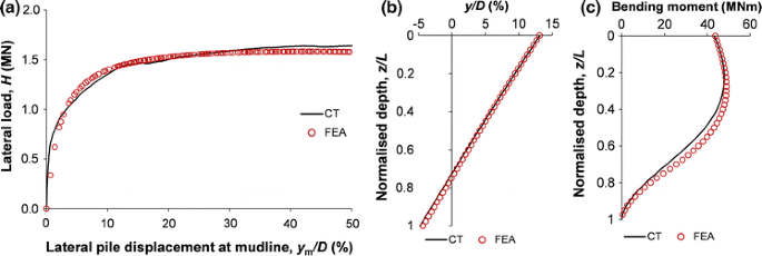

  

  Model verification. a Lateral load-displacement curve, b lateral pile displacement profile at $y_{\text{a}}$ = 1.61 m, c pile bending moment profile at $y_{\text{a}}$ = 1.61 m

• Analysis, using Model 3, illustrated in Fig. 1c, of a 7.5 m diameter steel monopile embedded 30 m in soft normally consolidated clay with $s_{u}$ ranging from 5 kPa at mudline to 67.6 kPa at the pile tip. $H$ and $M_{\text{a}}$ of 7.2 MN and 259.2 MNm respectively were applied to the pile in 100 equally spaced increments. The total stress approach was utilised with the clay assumed to be undrained and modelled by the Tresca yield criterion.

In these analyses, the clays were assumed to be linear elastic and their stiffness was correlated to the corresponding undrained shear strength using the Duncan and Buchignani (1976) procedure, which was calibrated using the simulation of centrifuge test CT by Model 2. The pile material was modelled as elastic-perfectly plastic; however, it remained elastic throughout the analysis as the stresses did not exceed the yield strength.

Although pile driving would lead to soil disturbance, it was assumed that this would be limited to a relatively thin region of soil around the pile in comparison to the much thicker zone of soil that would be subject to an increase in stress due to lateral loading. Therefore, pile installation was not modelled in these analyses.

Models with varying clay properties, element types, loading conditions and soil constitutive models were selected to ensure unbiased findings. Quadratic elements were not used as they brought about a negligible increase in solution accuracy that was offset by greater computational cost (Haiderali 2015). A fine mesh of between 27,072 and 255,936 elements, verified to be sufficiently accurate via a mesh sensitivity study (Haiderali 2015), was used. Finite sliding surface-to-surface contact pair formulation was used to accurately model the pile-soil interaction necessary for the computation of the soil resistance. In the normal direction, no contact stress was transmitted unless the pile nodes came into contact with the soil surface whilst in the tangential direction, the contact shear stress was related to the normal stress by the interface friction coefficient, $\mu$ (Coulomb friction law).

Pile bending moment profiles obtained via finite element analyses were truncated at a discrete number of locations to simulate strain-gauged piles. To determine optimum strain gauge positioning, 8, 4 and 6 distinct idealised strain gauge layouts corresponding to the 0.61, 3.8 and 7.5 m diameter piles, illustrated in Figs. 3, 4 and 5 respectively, were designed. These strain gauge layouts are referred to using their abbreviated notation, e.g. 6-SG denotes a layout with 6 strain gauges. The following rationale was applied in their design:

Fig. 3

Strain gauge layouts for the 0.61 m diameter pile. a 6-SG, b 7-SG, c 9-SG, d 11-SG, e 12-SG, f 12B-SG, g 15-SG, h 18-SG (not to scale)

Fig. 4

Strain gauge layouts for the 3.8 m diameter monopile. a Instrumented centrifuge model pile with six pairs of strain gauges (Lau 2015). b 6-SG identical to the model pile. c 7-SG, d 10-SG, e 11-SG (not to scale)

Fig. 5

Strain gauge layouts for the 7.5 m diameter monopile. a 6-SG, b 7-SG, c 10-SG, d 11-SG, e 15-SG, f 16-SG (not to scale)

• To ensure that the sectional properties of the piles used in experimental research would not be adversely affected, the maximum number of idealised strain gauges was limited to 18, 11 and 16 for the 0.61, 3.8 and 7.5 m diameter piles respectively, in proportion to their corresponding embedded lengths.

• Strain gauges were positioned to be roughly equidistant along the pile for the 3.8 and 7.5 m diameter piles, and for layouts 6, 9 and 12-SG for the 0.61 m diameter pile (Fig. 3a, c, e respectively). Since the deformation of the 0.61 m diameter pile was found by Haiderali and Madabhushi (2012) to be confined to its upper portion, layouts 11, 15 and 18-SG, shown in Fig. 3d, g, h, were designed to have a higher concentration of strain gauges within this segment of the pile.

• Layout 6-SG for the 3.8 m diameter monopile reproduced, at prototype scale, the strain gauge layout used for the centrifuge model monopile, shown in Fig. 4a, to enable the impact of curve fitting errors on p–y curves derived using centrifuge test results to be assessed.

• Based on the conventional assumption that the bending moment at the pile tip, $M_{\text{tip}}$, is zero, a dummy data point prescribed with this condition at the pile tip was included in all the strain gauge layouts for the 0.61 m diameter pile, the 6 and 10-SG layouts for the 3.8 m diameter pile (Fig. 4b, d respectively), and the 6, 10 and 15-SG layouts for the 7.5 m diameter pile (Fig. 5a, c, e respectively). However, it was found by Haiderali (2015) that large diameter piles have non-zero $M_{\text{tip}}$ due to the restraint provided by the soil. The effect of the zero $M_{\text{tip}}$ assumption on curve-fitting accuracy for the 3.8 and 7.5 m diameter piles was therefore assessed by not employing a dummy point with this condition at the pile tip but by instead including an additional strain gauge at the pile tip in the 7 and 11-SG layouts for the 3.8 m diameter pile (Fig. 4c, e respectively) and the 7, 11 and 16-SG layouts for the 7.5 m diameter pile (Fig. 5b, d, f respectively). It is assumed that strain gauges at the pile tip can be calibrated experimentally.

• Considering the bending moment in the lower half of the 0.61 m diameter pile tends to be negligible (Haiderali and Madabhushi 2012), layouts 7-SG and 12B-SG, illustrated in Fig. 3b, f respectively, were each designed to have 4 dummy points, between a depth of 20 and 35 m, at which the bending moment was specified to be zero.

Scripts were developed using MATLAB (2014) to automate curve fitting and numerical differentiation and integration operations at 100 load increments for the 0.61 and 0.75 m diameter piles, and 60 for the 3.8 m diameter pile. It is to be noted that the effect of strain gauge measurement errors on the accuracy of p–y curves is not covered in this study.

Curve Fitting Methods

In the context of this paper, curve fitting methods refer to both approximation and interpolation techniques. They were implemented using readily available software and are reproducible.

Given a bending moment data set having ($n + 1$) data points, ($z_{\text{i}}$, $M_{\text{i}}$), where no two $z_{\text{i}}$ are the same, there is a single (global) and unique $n$th degree interpolating polynomial, $f\left( z \right)$, that passes exactly through each of these data points. Mathematically, this is represented as

$$f\left( z \right) = a_{n} z^{n} + a_{n - 1} z^{n - 1} + \cdots + a_{2} z^{2} + a_{1} z + a_{0}$$

(3)

$$f\left( {z_{i} } \right) = M_{i} ,\quad i = 0, \ldots ,n$$

(4)

where $a_{0} , a_{1} , \ldots ,a_{n}$ are polynomial coefficients.

Due to the exactness of $f\left( z \right)$ at each data point, at high values of $n$, the interpolating polynomial manifests Runge’s phenomenon, which is defined as the oscillatory behaviour of the polynomial between the data points, especially towards the edges of the interval. To mitigate this, least squares approximation is undertaken to fit ($n + 1$) data points with a global polynomial of degree less than $n$. For this study, as detailed in Table 2, 3rd to 10th degree global polynomials were fitted by least squares approximation using the function polyfit. However, it is to be noted that where an $n$th degree polynomial was used to fit ($n + 1$) data points, polyfit generated an interpolating polynomial.

Table 2 Global polynomials analysed

An alternative approach is to apply a piecewise interpolating 3rd degree polynomial, known as a cubic spline, to each sub-interval, $\left[ {z_{i} , z_{i + 1} } \right]$, between the ($n + 1$) data points, for $i = 0, 1, \ldots ,n - 1$. The cubic spline function, ${\text{s}}_{i} \left( z \right)$, is computed for each sub-interval and represented mathematically as

$$s_{i} \left( z \right) = a_{i} + b_{i} \left( {z - z_{i} } \right) + c_{i} \left( {z - z_{i} } \right)^{2} + d_{i} \left( {z - z_{i} } \right)^{3}$$

(5)

where $a_{i}$, $b_{i}$, $c_{i}$ and $d_{i}$ are coefficients of the cubic spline function.

The cubic spline segments interconnect at the ($n + 1$) data points, also referred to as knots. The cubic spline function provides interpolation, slope (first derivative) and curvature (second derivative) continuity, as defined by Eqs. (6) to (8) respectively. A cubic spline has breaks at the data points.

$$s_{i} \left( {z_{i} } \right) = y_{i} ,\quad s_{i} \left( {z_{i + 1} } \right) = M_{i + 1} \quad {\text{for}}\;\;i = 0, \ldots ,n - 1$$

(6)

$$s_{i}^{{\prime }} \left( {z_{i + 1} } \right) = s_{i + 1}^{{\prime }} \left( {z_{i + 1} } \right)\quad {\text{for}}\;\;i = 0, \ldots ,n - 2$$

(7)

$$s_{i}^{{\prime \prime }} \left( {z_{i + 1} } \right) = s_{i + 1}^{{\prime \prime }} \left( {z_{i + 1} } \right)\quad {\text{for}}\;\;i = 0, \ldots ,n - 2$$

(8)

The interp1: spline function was used to interpolate the data with cubic splines having the ‘Not-a-knot’ boundary condition in which, as defined in Eq. (9), the third derivative was constrained to be continuous at the second and penultimate knots.

$$s_{0}^{{{\prime \prime \prime }}} (z_{1} ) = s_{1}^{{{\prime \prime \prime }}} (z_{1} ),\quad s_{n - 2}^{{{\prime \prime \prime }}} (z_{n - 1} ) = s_{n - 1}^{{{\prime \prime \prime }}} (z_{n - 1} )$$

(9)

Cubic splines eliminate oscillations associated with Runge’s phenomenon and being of a lower degree lead to a reduction in round-off errors as well.

Continuity between adjacent spline segments can also be obtained using Basis Splines, commonly known as B-splines. B-splines, which can be used for either approximation or interpolation, provide improved shape control and smoother derivatives in comparison to cubic splines as they satisfy the convex hull property. For a data set with n + 1 control points ($i = 0, \ldots ,n$), a B-spline of degree ($k - 1$) can be defined by Eq. (10):

$$s\left( z \right) = \mathop \sum \limits_{i = 0}^{n} N_{i,k} \left( z \right)P_{i}$$

(10)

where $s\left( z \right)$ is the B-spline function, $P_{i}$ is the knot vector, and $N_{i,k} \left( z \right)$ is the ith basis function of order $k$.

Interpolation with cubic, quartic (4th degree) and quintic (5th degree) B-splines was undertaken using the spapi function. A non-decreasing uniformly-spaced knot vector was specified using the aptknt (acceptable knot) algorithm. These B-splines, together with the cubic spline, were analysed at all the strain gauge layouts considered in this study.

The fitted bending moment curve was numerically double differentiated using the divided difference function diff to estimate the soil resistance profile, and double integrated using the trapezoidal integration function cumtrapz to obtain the lateral pile displacement profile. The solution of the two unknown integration constants required the prescription of two boundary conditions. Knowing that the deflection of the 0.61 m diameter pile is restricted to the upper part of its embedded length (Haiderali and Madabhushi 2012), its lateral displacement and slope (first integral of the bending moment) were specified to be zero at the pile tip. However, these boundary conditions were not appropriate for large diameter piles, which behave as rigid piles with a single but variable zero deflection point at which the soil resistance is also zero (Haiderali 2015). Hence, for the 3.8 and 7.5 m diameter piles, the lateral pile displacement was

• specified to be zero at the pile depth at which the soil resistance was interpolated to be zero, and

• at mudline, was equated to the FEA-derived value, since it could be measured during an experiment.

Curve Fitting Accuracy

The relative accuracy of the curve fitting techniques and strain gauge layouts was assessed using a combination of quantitative and qualitative measures. Quantitatively, the accuracy of the bending moment, lateral pile displacement and soil resistance profiles was evaluated by computing the normalised root mean square error (NRMSE),

$${\text{NRMSE}}\left( {\text{\% }} \right) = \left( {\sqrt {\frac{1}{{\left( {m \times n} \right)}}\mathop \sum \limits_{i = 1}^{m} \mathop \sum \limits_{i = 1}^{n} \left( {\zeta_{i} - \hat{\zeta }_{i} } \right)^{2} } \Big/\left( {\zeta_{ \hbox{max} } - \zeta_{ \hbox{min} } } \right)} \right) \times 100$$

(11)

where $m$ is the number of load increments: 100 for the 0.61 and 7.5 m diameter piles and 60 for the 3.8 m diameter monopile, $n$ is the number of locations along the pile at which comparisons between curve fitted and FEA-derived variables were performed: 36, 41 and 61 for the 0.61, 3.8 and 7.5 m diameter piles respectively (dependent on the vertical dimension of the elements), $\hat{\zeta }_{i}$ is the curve fitted variable ($\hat{M}_{i}$, $\hat{p}_{i}$ and $\hat{y}_{i}$), $\zeta_{i}$ is the FEA-derived variable ($M_{i}$, $p_{i}$ and $y_{i}$), and $\zeta_{ \hbox{max} }$ and $\zeta_{ \hbox{min} }$ are the maximum and minimum values of the FEA-derived variable for the entire sample.

Slight differences in the depth of the pivot point computed using FEA and derived via curve fitting exacerbated NRMSE at those locations. Although these errors could have been classified as ‘outliers’ and discarded from the sample, they were retained to ensure the error analysis was unbiased.

Qualitatively, the curve-fitted profiles were compared to equivalent FEA-derived profiles to examine the closeness of fit and identify variations in the displayed trend. Since every profile could not be visually examined, the root mean square error for all $n$ at a given load increment, ${\text{RMSE}}_{\text{Load}}$, defined in Eq. (12), was computed to enable profiles with the maximum, minimum and average error to be identified and inspected. Since the difference between $\zeta_{ \hbox{max} }$ and $\zeta_{ \hbox{min} }$ generally increased with loading, NRMSE was unsuitable for this purpose as it skewed the error.

$${\text{RMSE}}_{\text{Load}} = \sqrt {\frac{1}{n}\mathop \sum \limits_{i = 1}^{n} \left( {\zeta_{i} - \hat{\zeta }_{i} } \right)^{2} }$$

(12)

The relative accuracy of the curve fitting methods/strain gauge layouts in deriving p–y curves was judged by calculating the cumulative NRMSE for $p$ and $y$.

Digitisation of Curve-Fitted Bending Moment Curves

As stated in Sect. 1, after the bending moment data has been fitted using a particular function, the fitted curve is digitised to generate additional intermediate values on the curve to enhance the accuracy of subsequent numerical differentiation and integration. To determine the optimum number of digital data points required, a parametric study was undertaken using the cubic spline method and the 7-SG layout for the 7.5 m diameter pile. Listed in Table 3, an increase in the number of digital points from 601 to 14,401 resulted in a negligible increase in accuracy of $M$, $p$ and $y$. Additionally, even though double precision was used, severe errors in $y$, attributed to truncation, resulted when higher degree (8th to 10th) global polynomials were used with 9601 points. Consequently, 1201 digital points were considered optimum for the 7.5 m diameter pile. For the 0.61 and 3.8 m diameter piles, the number was adjusted to 1401 and 801 respectively to be proportionate to their embedded length.

Table 3 Parametric study undertaken to optimise the number of digital points

Results and Discussion

Small Diameter Pile

The trend displayed by the FEA-derived bending moment profiles was generally replicated by all the curve fitting methods. However, on closer inspection of the curve-fitted profiles, the following became evident:

• Across the methods, there was significant variance within the upper 6–7 m of the pile, especially between 0–2 and 5–7 m, at which sharp changes in the slope of the bending moment curve occurred.

• Global polynomials, at all the strain gauge layouts, exhibited considerable oscillation in comparison to the cubic spline and B-splines. This is illustrated in Fig. 6a for 6-SG 3rd degree and 11-SG 6th degree polynomials. The only exceptions were the curve-fitted profiles for 12-SG 8th to 10th degree polynomials, in which the fluctuation was not as significant. However, as the degree of the polynomial increased, incidence of Runge’s phenomenon, as shown in Fig. 6b for the 18-SG 10th degree polynomial, was manifested through large oscillations at the edge of the profiles.

  Fig. 6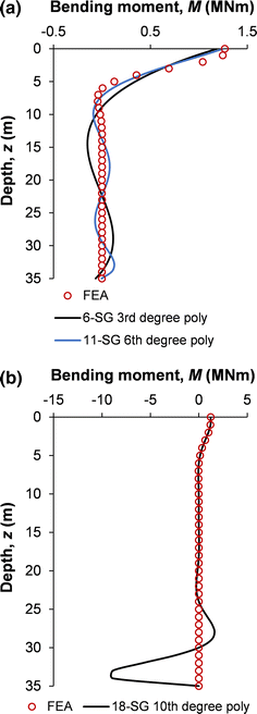

  

  Oscillation in fitted bending moment profiles for the 0.61 m diameter pile. a 6-SG 3rd degree and 11-SG 6th degree polynomials, b 18-SG 10th degree polynomial

• The accuracy of cubic spline and B-spline methods at 6-SG, illustrated in Fig. 7a, was relatively low with NRMSE of 5–6 % in its fitted profiles in comparison to the other strain gauge layouts in which NRMSE did not exceed 1.9 %. It can therefore be inferred that the use of six strain gauges is not sufficient to accurately interpolate the bending moment profile of a small diameter pile of this embedded length.

  Fig. 7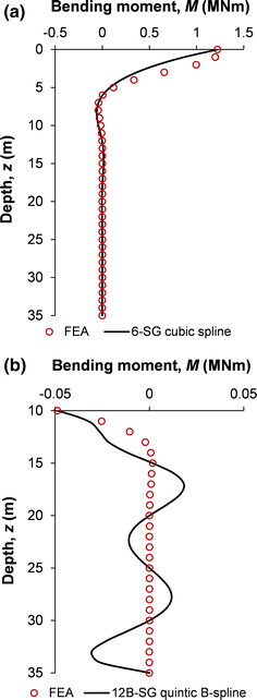

  

  Inaccuracies in fitted bending moment profiles for the 0.61 m diameter pile. a 6-SG cubic spline, b 12B-SG quintic B-spline

• The use of B-splines did not lead to the expected improvement in accuracy relative to cubic splines. On the contrary, as the degree of the B-spline increased, the accuracy became slightly diminished. As shown in Fig. 7b, oscillatory behaviour albeit slight was detected in the lower portion of the profile curve-fitted with the 12B-SG quintic B-spline.

• The most accurate profiles, with NRMSE less than 0.04 %, were obtained using cubic splines, cubic B-splines and quartic B-splines with the 12B-SG, 15-SG and 18-SG strain gauge layouts. Illustrated in Fig. 8 for the 12B-SG cubic spline and 18-SG quartic B-spline, the entire curve was accurately represented by these methods. Furthermore, the increase in accuracy between 12B-SG and 18-SG was trivial indicating the superiority of 12B-SG in which fewer strain gauges, concentrated along the upper part of the pile, were used in conjunction with multiple dummy points along the lower portion of the pile at which the bending moment was specified to be zero.

  Fig. 8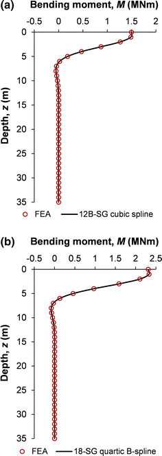

  

  Accurate bending moment profiles for the 0.61 m diameter pile. a 12B-SG cubic spline, b 18-SG quartic B-spline

Shown in Fig. 9a, oscillations in bending moment caused by the global polynomials resulted in their lateral pile displacement profiles having large errors. In particular, NRMSE was extremely high, in the range between 208 and 4973 % for the 8th to 10th degree polynomials at 15 and 18-SG layouts, due to over-fitting of the bending moment data. However, profiles derived using 5th to 10th degree polynomials displayed improved accuracy at the equidistant strain gauge layouts 6-SG, 9-SG and 12-SG, with NRMSE ranging between 3.8 and 11.9 %. This is illustrated in Fig. 9b for 12-SG 7th, 8th and 10th degree polynomials.

Fig. 9

Lateral pile displacement profiles for the 0.61 m diameter pile derived using global polynomials. a Highly inaccurate with 7-SG 3rd, 12B-SG 5th and 18-SG 6th degree polynomials, b improved accuracy with 12-SG 7th, 8th and 10th degree polynomials

In contrast, lateral pile displacement profiles derived using the splines were much more accurate with NRMSE varying between 1.8 and 8.4 %. Similar to the earlier findings, 12B-SG proved to be just as accurate as layouts with a higher number of strain gauges. Interestingly though, as shown in Fig. 10a, relatively accurate profiles were also obtained with the 6-SG layout whose bending moment profiles had exhibited slightly larger errors in comparison to the other strain gauge layouts. In addition, the spline accuracy with the 9 and 12-SG layouts was higher than expected and was not reflective of the errors in their corresponding bending moment profiles. Hence, it can be conjectured that the trapezoidal integration procedure is oblivious to small errors in the bending moment profile and that its accuracy is enhanced when strain gauges are positioned to be near-equidistant. Although the use of quartic B-splines resulted in only a slight reduction in accuracy of the lateral displacement profiles relative to cubic B-splines, the loss of accuracy was considerable with quintic B-splines (Fig. 10b).

Fig. 10

Lateral pile displacement profiles for the 0.61 m diameter pile derived using splines. a 6-SG and 12B-SG cubic splines, b 7-SG and 18-SG quintic B-splines

In comparison, numerical differentiation of the bending moment curves was highly susceptible to errors resulting in significant differences in the soil resistance profiles derived using the curve fitting methods and those predicted by FEA. The global polynomials, as expected, performed poorly with their soil resistance profiles deviating significantly from the required trend (Fig. 11a). As a result, their NRMSE was between 13.1 and 117.9 % for the 3rd to 9th degree polynomials and in excess of 900 % for the 10th degree polynomial. However, the closeness of fit for the 7th to 10th degree polynomials at 12-SG was much better, as shown in Fig. 11b, thus resulting in NRMSE in the range of 8.3–31.3 %, with the lower and higher bound values corresponding to the 7th and 10th degree polynomials.

Fig. 11

Soil resistance profiles for the 0.61 m diameter pile. a 18-SG 3rd, 5th and 8th degree polynomials, b 12-SG 7th, 8th and 10th degree polynomials, c 12B, 15 and 18-SG cubic splines, d 12B, 15 and 18-SG cubic B-splines

Soil resistance profiles derived using splines were of considerably higher accuracy, with NRMSE of 4.7-17.6 %. Cubic splines and cubic B-splines at 12B, 15 and 18-SG were the most accurate whereas all the splines at 6-SG were the least accurate. However, as shown in Fig. 11c, d, even the most accurate methods failed to capture the local maxima close to the soil surface. Finally, higher degree B-splines, especially quintic B-splines, were found liable to inaccuracies.

Assimilating these findings, cubic and cubic B-splines with 12B-SG, 15-SG and 18-SG strain gauge layouts, with cumulative NRMSE of 8.6 %, were determined to be the most accurate methods for deriving p–y curves. They were followed by 9-SG quartic B-spline (10.2 %), 9-SG quintic B-spline (12.1 %), 12-SG 7th degree polynomial (12.8 %), 15-SG quintic B-spline (14.1 %) and 12-SG 8th degree polynomial (16.8 %). A comparison of FEA-derived p–y curves and those obtained via the 12B, 15 and 18-SG cubic spline methods, at depths of 1 and 5 m, is provided in Fig. 12.

Fig. 12

Comparison of p–y curves derived for the 0.61 m diameter pile using FEA and 12B, 15 and 18-SG cubic spline methods. a $z$ = 1 m, b $z$ = 5 m (p–y curves derived using the cubic B-spline method have been omitted for clarity)

Large Diameter Piles

Owing to the smoothness of the bending moment profiles for the 3.8 and 7.5 m diameter piles, all the methods yielded very accurate profiles that replicated the trend depicted by FEA. Oscillation between data points was not observed for the global polynomials, including the high degree ones. The following was deduced upon closer examination:

• Illustrated in Fig. 13a, b, the most accurate methods for the 3.8 m diameter pile were the 11-SG cubic spline and cubic B-spline with NRMSE of 0.04 % whereas those for the 7.5 m diameter pile were the 16-SG quintic B-spline and 10th degree polynomial with NRMSE of 0.02 %.

  Fig. 13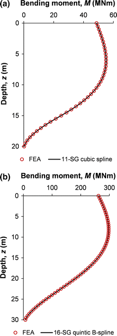

  

  Accurate bending moment profiles. a 11-SG cubic spline for the 3.8 m diameter pile, b 16-SG quintic B-spline for the 7.5 m diameter pile

• For both piles, the 3rd and 4th degree polynomials were the least accurate with NRMSE of between 1.1 and 3.4 % (Fig. 14a).

  Fig. 14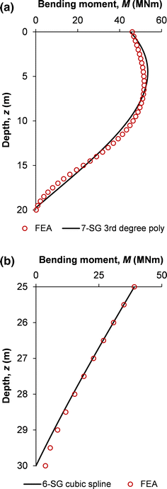

  

  Inaccuracies in bending moment profiles. a 7-SG 3rd degree polynomial for the 3.8 m diameter pile, b 6-SG cubic spline for the 7.5 m diameter pile

• As shown in Fig. 14b, the inaccuracy arising from the assumption of zero ${\text{M}}_{\text{tip}}$ in the 7.5 m diameter pile was not limited to the pile tip but extended up to a depth of 28 m.

Similarly, a majority of the methods predicted lateral pile displacement profiles with relatively high accuracy. Best performing methods for the 3.8 m diameter pile were the 11-SG 8th degree polynomial, 7-SG cubic B-spline and the 11-SG quintic B-spline with corresponding NRMSE of 0.08, 0.10 and 0.11 % (Fig. 15a). The least accurate were the 3rd and 4th degree polynomials with NRMSE of 6.33–146.86 % (Fig. 15b). With the exception of the 3rd degree polynomials, which were relatively inaccurate with NRMSE of 2.44–3.06 % (Fig. 15c), lateral pile displacement profiles for the 7.5 m diameter pile were derived to be consistently accurate. NRMSE varied between 0.27 % for the 16-SG 6th degree polynomial (Fig. 15d) and 0.65 % for the 7-SG cubic and cubic B-splines. The reduction in accuracy due to the use of the zero ${\text{M}}_{\text{tip}}$ dummy point, when averaged across all the methods, was 0.1 % for both piles. This confirms the hypothesis that the numerical integration procedure is insensitive to slight errors in the bending moment curve.

Fig. 15

Lateral pile displacement profiles. a $D$ = 3.8 m, 11-SG 8th degree polynomial, b $D$ = 3.8 m, 11-SG 4th degree polynomial, c $D$ = 7.5 m, 7-SG 3rd degree polynomial, d $D$ = 7.5 m, 16-SG 6th degree polynomial

Analogous to the findings for the 0.61 m diameter pile, the numerical differentiation procedure was found to be error-prone resulting in inaccuracies in the soil resistance profiles for the large diameter piles. A comprehensive examination indicated the following:

• The variance between profiles derived using these methods and FEA was mainly in the upper 2–3 m and the lower 3-5 m of the pile. With most of the methods, a distinction could not be made along the rest of the pile.

• The most accurate methods for the 3.8 m diameter pile were the 7-SG cubic and cubic B-splines with NRMSE of 3.8 and 4 % respectively. The accuracy of profiles derived using the 6-SG cubic and cubic B-splines was also similar indicating the effect of assuming zero bending moment at the pile tip to be insignificant (Fig. 16a). This was not entirely unexpected considering the magnitude of $M_{\text{tip}}$ was quite small for this monopile.

  Fig. 16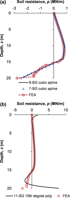

  

  Soil resistance profiles for the 3.8 m diameter pile. a 6 and 7-SG cubic splines, b 11-SG 10th degree polynomial

Interestingly, there was no gain in accuracy by increasing the number of strain gauges to 10/11.

The least accurate methods were the 10 and 11-SG 10th degree polynomials with NRMSE in excess of 40 % (Fig. 16b). It was also noted that the use of 4th and 5th degree B-splines aggravated these inaccuracies.

• For the 7.5 m diameter pile, illustrated in Fig. 17, the 16-SG 10th degree polynomial and the 3rd degree polynomial at all three strain gauge layouts (7, 11 and 16-SG) were the most and least accurate respectively with corresponding NRMSE of 3.1 and 8.1 %. However, the overall margin of error was quite low with the rest of the methods having NRMSE of between 3.2 and 4.7 %.

  Fig. 17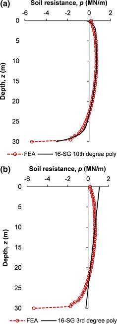

  

  Soil resistance profiles for the 7.5 m diameter pile. a 16-SG 10th degree polynomial, b 16-SG 3rd degree polynomial

Unlike the 3.8 m diameter pile, the use of a dummy point with zero $M_{\text{tip}}$ had a more profound effect on the accuracy of the soil resistance profiles. For instance, as shown in Fig. 18a, the 15-SG cubic spline predicted soil resistance at the pile tip that was completely opposite to the FEA-depicted trend. Hence, use of a strain gauge at the pile tip is recommended for the 7.5 m diameter monopile.

Fig. 18

a Inaccuracies in the soil resistance profile when ${\text{M}}_{\text{tip}}$ is assumed to be zero using 15-SG cubic spline, b verification of FEA soil resistance output

• The sharp increase in soil resistance at the tip of the 7.5 m diameter pile was not accurately depicted by any of the methods used. To confirm that this was not due to an over-estimation in FEA, the analysis was repeated using the augmented Lagrangian contact enforcement algorithm, which is considered to be more accurate than the penalty stiffness method used in the current analyses. However, as shown in Fig. 18b, the soil resistance curves derived from these analyses were identical. Therefore, it is concluded that the inability to predict this phenomenon is not due to deficiencies in the curve fitting methods but rather exposes the underlying limitations of the p–y method in modelling extremely large diameter monopiles.

Incorporating these findings, the most accurate methods for deriving p–y curves for the 3.8 m diameter pile were the 6/7-SG cubic B-splines and cubic splines with cumulative NRMSE of 3.8 and 4.1 % respectively. They were closely followed by the 10/11-SG cubic B-splines and cubic splines with cumulative NRMSE of 5.3 %. Therefore, the 6-SG layout used by Lau (2015) in the centrifuge test is considered optimum for this monopile. Regarding the 7.5 m diameter pile, all methods except the 3rd degree polynomials yielded relatively accurate p–y curves with cumulative NRMSE not exceeding 5.5 %. The top-ranked methods, listed in Table 4, point to the 16-SG layout as being the optimum layout. Figure 19 shows p–y curves, at depths of 5 and 10 m, for the 3.8 and 7.5 m diameter monopiles.

Table 4 Ranking of most accurate methods for the 7.5 m diameter monopile

Fig. 19

p–y curves. a $D$ = 3.8 m, $z$ = 5 m, b $D$ = 3.8 m, $z$ = 10 m, c $D$ = 7.5 m, $z$ = 5 m, d $D$ = 7.5 m, $z$ = 10 m

Although the optimum strain gauge layout would vary depending on pile characteristics, on the basis of this study, the cubic spline and cubic B-spline methods were found to be consistently accurate for the full range of laterally loaded piles. This is particularly important for piles that are difficult to categorise prior to an experiment, for instance, hybrid monopiles, piles in novel geomaterials, etc.

Conclusions

Derivation of p–y curves from experimental research is reliant on curve fitting techniques whose accuracy and reliability is subject to uncertainties. To provide guidance on the optimum positioning of strain gauges and the choice of curve fitting methods for deriving p–y curves for laterally loaded piles in clay, a comparison was carried out between 3D FEA results and cubic spline, cubic to quintic B-spline and 3rd to 10th degree global polynomial techniques at 18 strain gauge layouts. Its key findings were:

• Fitting bending moment data for the small diameter pile was more challenging due to sharp changes in the slope of the bending moment profile. As a result, global polynomials generally performed poorly. In contrast, due to the bending moment curve of the large diameter piles being fairly smooth, all the methods considered, including the high degree polynomials, were relatively accurate.

• For both pile categories, the numerical integration procedure was found to be insensitive to small errors in the fitted bending moment curve. On the other hand, the numerical differentiation procedure was error-prone resulting in the amplification of slight errors in the bending moment profile. Hence, soil resistance profiles for the small diameter pile had significantly larger errors that those for the large diameter piles.

• Irrespective of the method or strain gauge layout used, the sharp increase in soil resistance at the tip of the 7.5 m diameter pile could not be derived. This was attributed to the failure of the p–y method in modelling the development of shear at the pile tip and the consequent increase in soil resistance.

• For monopiles greater than 3.8 m in diameter, it is advisable to include a strain gauge at the pile tip as inaccuracies were noticeable when the bending moment there was assumed to be zero. However, for the 3.8 m diameter pile, this assumption had no accuracy implications.

• For the small diameter pile, a strain gauge layout with a higher concentration of strain gauges within the upper third of the pile coupled with multiple dummy points with zero bending moment along the rest of the pile was found to be optimum. Such a strain gauge layout would also require fewer strain gauges and therefore minimise adverse effects on the sectional and surface properties of the pile.

• An increase in the number of strain gauges for the large diameter piles did not lead to a significant increase in accuracy.

• Across the full range of laterally loaded piles, cubic and cubic B-splines were found to be most consistent.

References

Barton YO (1982) Laterally loaded model piles in sand. PhD Dissertation, University of Cambridge
Bouafia A, Bouguerra A (2006) Single piles under lateral loads—centrifuge modelling of some particular aspects. In: Proceedings of the international conference on physical modelling in geotechnics, Hong Kong, pp 915–920
Bouafia A, Garnier J (1991) Experimental study of p–y curves for piles in sand. In: Ko H, McLean FG (eds) Centrifuge 91. Balkema, Rotterdam, pp 261–268
Choo YW, Kim D (2015) Experimental development of the p–y relationship for large-diameter offshore monopiles in sands: centrifuge tests. J Geotech Geoenviron Eng 04015058:1–12
Dassault Systèmes (2011) “Abaqus/standard version 6.11-1.” Computer program. Dassault Systèmes Simulia Corp, Providence
Dassault Systèmes (2012) “Abaqus/Standard Version 6.12-2.” Computer program. Dassault Systèmes Simulia Corp, Providence
Duncan JM, Buchignani AL (1976) An engineering manual for settlement studies. Report, Berkeley
Dyson GJ, Randolph MF (1998) “Installation effects on lateral load-transfer curves in calcareous sands. In: Kimura T, Kusakabe O, Takemura J (eds) Centrifuge 98, vol 1. Balkema, Rotterdam, pp 545–550
Ellis EA (1997) Soil-structure interaction for full-height piled bridge abutments constructed on soft clay. PhD Dissertation, University of Cambridge
Haiderali AE (2015) Numerical modelling of monopiles for offshore wind farms. PhD Dissertation, University of Cambridge
Haiderali AE, Madabhushi SPG (2012) Three-dimensional finite element modelling of monopiles for offshore wind turbines. In: Proceedings of the world congress on advances in civil, environmental, and materials research, Seoul, pp 3277–3295
Ilyas T, Leung CF, Chow YK, Budi SS (2004) Centrifuge model study of laterally loaded pile groups in clay. J Geotech Geoenviron Eng 130(3):274–283
Jeanjean P (2009) Re-assessment of p–y curves for soft clays from centrifuge testing and finite element modelling (OTC-20158-MS). In: Offshore technology conference, Houston
King GJW (1994) “The interpretation of data from tests on laterally loaded piles. In: Leung CF, Lee FH, Tan ETS (eds) Centrifuge 94. Balkema, Rotterdam, pp 515–520
Kitazume M, Miyajima S (1994) Lateral resistance of a long pile in soft clay. In: Leung CF, Lee FH, Tan ETS (eds) Centrifuge 94. Balkema, Rotterdam, pp 485–490
Klinkvort RT (2012) Centrifuge modelling of drained lateral pile–soil response: application for offshore wind turbine support structures. PhD Dissertation, Technical University of Denmark
Kong LG, Zhang LM (2007) Rate-controlled lateral-load pile tests using a robotic manipulator in centrifuge. Geotech Test J 30(3):1–10
Lau BH (2015) Cyclic behaviour of monopile foundations for offshore wind turbines in clay. PhD Dissertation, University of Cambridge
MATLAB (2014) MATLAB Version 2014b. Computer Program. The MathWorks Inc., Natick
Matlock H (1970) Correlations for design of laterally loaded piles in soft clay (OTC 1204). In: Offshore technology conference, pp 577–594
Mezazigh S, Levacher D (1998) Laterally loaded piles in sand: slope effect on p–y reaction curves. Can Geotech J 35(3):433–441
Reese LC, Welch RC (1975) Lateral loading of deep foundations in stiff clay. J Geotech Eng Div 101(GT7):633–649
Reese LC, Cox WR, Koop FD (1974) Analysis of laterally loaded piles in sand (OTC 2080). In: Offshore technology conference, Dallas, pp 473–483
Reese LC, Cox WR, Koop FD (1975) Field testing and analysis of laterally loaded piles in stiff clay (OTC 2321). In: Offshore technology conference, Houston, pp 671–690
Remaud D, Garnier J, Frank R (1998) “Laterally loaded piles in dense sand: group effects. In: Kimura T, Kusakabe O, Takemura J (eds) Centrifuge 98, vol 1. Balkema, Rotterdam, pp 533–538
Springman SM (1989) Lateral loading on piles due to simulated embankment construction. PhD Dissertation, University of Cambridge
Yang K, Liang R (2006) Methods for deriving p–y curves from instrumented lateral load tests. Geotech Test J 30(1):1–8
Acknowledgments
The first author is grateful to University of Cambridge and the Engineering and Physical Sciences Research Council for the doctoral scholarship.
Author information
Authors and Affiliations
Corresponding author
Rights and permissions
Open Access This article is distributed under the terms of the Creative Commons Attribution 4.0 International License (http://creativecommons.org/licenses/by/4.0/), which permits unrestricted use, distribution, and reproduction in any medium, provided you give appropriate credit to the original author(s) and the source, provide a link to the Creative Commons license, and indicate if changes were made.
About this article
Cite this article
Haiderali, A.E., Madabhushi, G. Evaluation of Curve Fitting Techniques in Deriving p–y Curves for Laterally Loaded Piles. Geotech Geol Eng 34, 1453–1473 (2016). https://doi.org/10.1007/s10706-016-0054-2
Received:
Accepted:
Published:
Issue Date:
DOI: https://doi.org/10.1007/s10706-016-0054-2