
Abstract
Cloud computing platforms have been continuously evolving. Features such as the Elastic Fabric Adapter (EFA) in the Amazon Web Services (AWS) platform have brought yet another revolution in the High Performance Computing (HPC) world, further accelerating the convergence of HPC and cloud computing. Other public clouds also support similar features further fueling this change. In this paper, we show how and why the performance of a large-scale computational fluid dynamics (CFD) HPC application on AWS competes very closely with the one on Beskow—a Cray XC40 supercomputer at the PDC Center for High-Performance Computing - in terms of cost-efficiency with strong scaling up to 2304 processes. We perform an extensive set of micro and macro benchmarks in both environments and conduct a comparative analysis. Until as recently as 2020 these benchmarks have notoriously yielded unsatisfactory results for the cloud platforms compared with on-premise infrastructures. Our aim is to access the HPC capabilities of the cloud, and in general to demonstrate how researchers can scale and evaluate the performance of their application in the cloud.
1 Introduction
Cloud computing has revolutionized the way computational resources are delivered by making them available on-demand and at a low cost. Consistent with the democratization of technology in this era of globalization, it has made computing power and data storage more affordable and accessible than ever before [1]. The existence of hundreds of cloud providers today attests to the massive success of cloud computing.
Small companies and individuals can now get access to the IT infrastructure they need without any investment in hardware and maintenance. It has considerably cut down the cost of IT and enabled companies to scale up with little effort compared with before. Naturally, the potential of using cloud service providers has widely attracted researchers’ attention, some of whom have conducted feasibility studies of moving their research in the cloud ([2,3,4] among the first). When it comes to large-scale high-performance computing applications, which is the topic of this paper, the question becomes the following. Can the performance of HPC applications in the cloud match the one in on-premises infrastructures?
In this paper, we pursue the idea of moving HPC in the cloud and provide a thorough performance analysis making use of the latest advances of AWS in the direction of HPC. However, the general procedure we outline to evaluate the performance of the application and the trends we describe could serve as blueprint for any comparative study of this type regardless of the cloud platform or on-premise infrastructure.
2 Literature review
According to the taxonomy of efforts in HPC presented by Netto et al. [5], the contribution of this paper is in the category of HPC in the cloud or specifically, viability studies of moving HPC to cloud environments. Early explorations have been initiated as early as in 2008. Studies from this early period of cloud computing such as the ones performed by Walker [2], Napper et al. [3] and Ostermann et al. [4] categorically concluded that the cloud is not yet mature for tightly coupled HPC applications.
In 2010, Amazon EC2 introduced the first generation of HPC infrastructure. However, various studies from 2010 [6,7,8,9], and more importantly 2011, still indicated that while the cloud is cost effective and delivers satisfactory performance for “low communication-intensive applications such as embarrassingly parallel and tree-structured computations” [10], it is still not mature enough for HPC applications. Zhai et al. [11] and the Magellan Report [12] both concluded that the lack of of a high performance network severely limits the execution of tightly-coupled HPC applications.
Numerous studies [13,14,15,16,17] from the period between 2012 and 2015 indicate that while cloud computing is not yet mature for HPC, the performance is becoming comparable. In particular, Mehrotra et al. in their “Performance evaluation of amazon EC2 for NASA HPC applications” [13], state that although the HPC performance in the AWS lags behind the one on their reference supercomputer due to the network technology and virtualization overhead, it is quickly catching up.
Starting from 2016 to 2018, feasibility studies [18, 19] suggest that a hybrid approach would make the most of the two environments, cloud and on-premise clusters, given that the network latency is still higher in the cloud [20, 21]. Despite this, Bartosz et al. [21] find that the elastic cloud can provide a better turnaround time, “reducing the time to science”. A comparative paper by Mohammadi also claims that “the performance on public cloud can be comparable to modern traditional supercomputing systems” [22]. In short, the outlook for HPC in the cloud brightens.
For a more complete literature review of feasibility studies in the cloud until 2018 we refer the readers to [5].
The needs of researchers regarding HPC have been heard and taken into account by cloud providers. In the case of Amazon, the result is the announcement of the RDMA/ EFA (Elastic Fabric Adapter) networking interface with up to 100 Gbps bandwidth, in 2019. Breuer et al. [23] show promising results for Seismic Simulations in the cloud and state that this new development, once released, is expected to further improve the strong scalability of their applications. Other promising studies include NASA’s evaluation of Azure cloud for HPC [24], Maliszewski’s study of interconnection in Azure Cloud [25, 26] and Guidi’s et al. [27] summary/survey on cloud perfomrance over the last ten years.
Finally, with the release of EFA, Zhuang et al. [28] show that Amazon EC2 achieves comparable performance to local supercomputing clusters for their GEOS-Chem atmospheric chemistry simulations, due to recent developments in the network performance and reduction of virtualization overhead. They dispute the validity of the paradigm that the cloud is not mature for HPC applications EFA is an effort in the direction of long-term cooperation with the industry, as highlighted by the MVAPICH project [29]. Fernandez [30] conducts the HPCG benchmark in five cloud platforms, highlighting among others the scalability of the C5n.18xlarge instances. The computational fluid dynamics (CFD) package, Ansys Fluent [31], also showcases the performance results for a benchmark on AWS EC2 of the external flow over a Formula-1 Race car with 140 million hex-core cells using the Finite Volume Metod (FVM). Similarly, Turner et al. [32] showcase the performance of a Reynolds Averaged Navier–Stokes (RANS) simulation of a full aircraft on Amazon EC2 c5n.18xlarge instances. In contrast, our application uses the Finite Element Method on tetrahedral meshes of a F1 Perrinn model, which is a conceptually different method to be compared directly. We also conduct thorough benchmarking in conjunction with the performance of the application.
Today practically all major public cloud providers offer HPC capabilities [33,34,35]. It is already a competitive established market that caters to a notable number of private companies (aerospace, automotive, biochemistry among many). In comparison, in literature one finds very few studies performed in academia showcase the performance of HPC applications since the introduced changes.
The largest bottleneck identified for running HPC applications right now in the cloud is the networking by large consensus [5, 12, 13, 23,24,25, 28, 36, 37]. Different clouds have addressed this problem to different degrees in reference to each other and internally based on the choice of node. De et al. [37] provide a very detailed study of the network performance using MPI benchmarks for various public clouds. The important takeaway relevant here is the fact that network noise for HPC nodes i.e. with at least 100 Gbps bandwidth is comparable to the one on-premise, further supporting the results we are about to present.
3 Goals and contributions
Networking, compute power and storage speed are the most important factors that impact the performance of scientific applications. Firstly, we benchmark these factors separately. Compute power and networking are the most relevant ones for our application. We then evaluate their impact on the performance of our massively parallel CFD application. Typically, applications are categorized into four main categories: compute-intensive, memory-intensive, data-intensive, and high-throughput. We should note that the application we selected is partly compute-intensive, partly memory-intensive. Therefore, networking and compute power have an especially strong impact on the performance. Researchers can use a wide range of tools to characterize their own applications (for example VTune Profiler [38]).
In this paper we report the results from benchmarking and examining the performance of HPC applications on Amazon EC2, using the open-source tool developed by AWS, ParallelCluster (released in November 2018 [39]). Relatively recent technological advancement such as the AWS Nitro Hyperviso, a very light hypervisor that removes a large part of the virtualization overhead, was introduced in 2017. The Elastic Fabric Adapter (EFA) feature is available in ParallelCluster as of April 2019 [40]. These technologies have largely made possible the results presented in the subsequent sections.
The contributions of this work are:
-
I
Thorough benchmarking using the OSU micro benchmarks and the NASA macro benchmarks. The results can be used as indicators to make predictions about the performance of HPC applications by other researchers who might want to migrate their research to the cloud.
-
II
Performance analysis of an HPC application consisting of strong scaling and profiling. This application represents a large class of problems that involve solving a system of non-linear PDEs, using the Newton method, solving a linear system of equations in each iteration. It generalizes to many scientific applications in different fields, discretized with the Finite Element method, with sparse systems of equations. In conjunction with I), we identify the underlying factors that lead to improved performance.
Both I) and II) are conducted in Amazon EC2 and on Beskow, a Cray XC40 supercomputer, followed by a comparative analysis. Throughout the process, we explain and highlight general trends that are relevant for these types of feasibility studies.
4 Configuration
Table 1 shows a summary of the hardware specifications of both environments discussed in this section, in terms of node compute power, memory configuration and networking.
In conjunction, we describe in detail the configuration of the two environments in which we have run both the benchmarks (micro and macro) and the HPC application. Simultaneously, we outline how to create an AWS EC2 cluster and which tools to use.
4.1 Amazon EC2 and AWS ParallelCluster
Amazon EC2 stands for Amazon Elastic Compute Cloud. It is one of the Amazon Web Services which offers users access to computational resources physically distributed in data centers across the globe.
ParallelCluster is an open-source, command-line tool developed by Amazon that enables a quick way to set up and manage a cluster in Amazon EC2 from a configuration file. It consists of various groups of configuration options or sections. Table 2 details a configuration that yields satisfactory performance for an initial exploration of the cloud’s capabilities with ParallelCluster v2. The latest version at the time of writing, v3, offers an interactive setup using either CLI or UI interface for the same options. For a full list of options, see the documentation for AWS ParallelCluster [41].
The C5n instances in Amazon’s Compute Optimized family are fit for computationally intensive workloads due to their Enhanced Network Bandwidth support for high-speed communication between nodes, taking advantage of the Nitro System and the Elastic Fabric Adapter (EFA) to deliver network bandwidth of 100 Gbps [40]. The EFA feature was introduced in 2019 [42], at which point the C5n instances were state-of-the-art. They remained so at the time of conducting this study and until the end of 2020 when new instances have been added to the Compute Optimized family i.e C6a, C6i, C6in, C6g, C6gn, and C7g [43]. AWS has also created a new HPC family that includes hpc6a and hpc6id, introduced at the end of 2021 and 2022 accordingly [44]. Since our reference cluster runs on Intel processors, in this study our aim was to get to as even baseline as possible as a first step, using machines with same bandwidth (100 Gbps) and type of processor (Intel). Next step would be to incrementally introduce extra layers of complexity by extending the study to Graviton and AMD architectures with same network bandwidth as the C5n nodes i.e. C6gn, and hpc6a respectively. The only candidates with network bandwidth not inferior or equal to 100 Gbps are C6in, C6id, and C7gn, all of them introduced at the end of 2022 with the optimized version of the EFA, that open new interesting possibilities to explore.
The C5n.x18large instances are equipped with two sockets x 18 Intel(R) Xeon(R) Platinum 8124 M CPU @ 3.00GHz (Skylake), a total of 72 vCPUs with Simultaneous Multithreading and 192 GiB of memory. Our configuration consists of up to 40 compute nodes, C5n.x18large type (max_queue_size setting). For the master node responsible for coordinating compute nodes, compiling code, and interacting with the job scheduler, we balance cost and performance by opting for a C5n.4xlarge instance. We utilize Ubuntu 18.04 as the base_os (see Table 2).
Amazon uses its proprietary Nitro System to create and manage virtual machines in the cloud. This system includes the light-weight Nitro Hypervisor, offloading hypervisor workload to dedicated components: Nitro Cards, and Nitro Security Chip. This reduces virtualization overhead - one of the major bottlenecks in the past, and improves performance [45].
The job scheduler handles job initiation, scheduling, and monitoring. The latest version of ParallelCluster provides several options for cluster schedulers, including Son of Grid Engine, Slurm Workload Manager, Torque Resource Manager, and AWS Batch. In the specific configuration mentioned in Table 2, Slurm is chosen as the scheduler, same as the reference supercomputer.
The HPC application we focus on in this paper makes use of the standardized Message Passing Interface (MPI). The choice of MPI implementation can impact the performance of your application dramatically. It is noteworthy to mention that alternatives to using MPI implementations, such as Chapel, UPC, UPC++, Spark, and others, might be worth looking into as well. Techniques such as multilevel parallelism [46] can further improve performance or algorithms that employ non-blocking MPI routines especially for Graviton and AMD based nodes with more compute power such as Hpc6a, C6gn, etc [47].
We have tested two MPI implementations on our cluster: Open MPI and Intel MPI. Both of them wrap around the open-source GNU compiler. The IntelMPI version available through AWS is the open-source version of the Intel MPI wrapper that wraps around the GNU compiler.
The placement of the nodes within a chosen time zone is also crucial. To minimize the distance between the nodes and achieve a low-latency network performance, we can use the placement group options available (placement_group in Table 2).
For storage, we utilize a 6000 GB gp2 SSD volume, providing a maximum of 16000 IOPS and a Max Throughput/Volume of 250 MB/s. This mid-range option offers both competitive pricing and performance, making it suitable for a diverse range of workloads.
The Nitro card for VPC supports several network acceleration features, such as EFA (it optimizes for latency between 2 instances, scaling elasticity). You can enable the EFA (a network device) option through the enable_efa flag in the configuration Table 2. RDMA (Remote Direct Memory Access) is a network protocol used to side-step the processor and exchange data between two main memories directly, bypassing the OS. We observed a significant impact using this feature in our results, which prompted us to write this paper.
Last but not least, the advances in load balancing, task scheduling, resource allocation, and distributed computing algorithms for network communication also play a significant role in the overall performance in the cloud. They facilitate the ability to have a reliable low communication latency between the nodes in a worldwide distributed system, a crucial factor in getting a good performance.
On the software side, we use the open-source Spack manager to manage the packages in a modular way [48, 49]. It allows for a quick installation of core dependencies we need to run our software, enabling different versions to coexist without any issue - an essential requirement in supercomputing environments.
4.2 Beskow—Cray XC40 supercomputer
Beskow [50], a Cray XC40 supercomputer, located at the PDC Center for High-Performance Computing in Stockholm, consists of 11 cabinets with a total of 2060 compute nodes and 67,456 cores. Each node contains 2 Intel CPUs:
-
9 cabinets with Xeon E5-2698v3 Haswell 2.3 GHz (16 cores/CPU)
-
2 cabinets with Xeon E5-2695v4 Broadwell 2.1 GHz(18 cores/CPU)
We have run the benchmarks and the simulations on the Xeon E5-2698v3 Haswell 2.3 GHz nodes. The nodes interconnect with a High-speed network Cray Aries (Dragonfly topology) that also supports RDMA operations.
The Haswell nodes have 64 GB of RAM, and the Broadwell nodes have 128GB. Beskow has in its disposal a 5 Petabyte Lustre file system.
Beskow achieves a peak performance of 2.438 Petaflops (\(10^{15}\) floating-point operations per second). The Linpack benchmark has a long-standing history as a criterion for ranking the top supercomputers. This benchmark solves dense systems of linear equations and naturally is not a reference for the performance of all kinds of applications. Beskow lists a Linpack performance of 1.80 Petaflops. Based on the type of application, we need a representative benchmark to obtain an accurate estimate of its performance.
Beskow also relies on Slurm as a scheduler. The results reported in this study have been obtained with the native Cray MPI implementation, the most optimized one for the underlying hardware.
5 Benchmarks
The microbenchmarks are small pieces of code that have the purpose of quantifying the basic building blocks of a program separately. The macro-benchmarks, on the other hand, consist of a more complex code that should be representative of the class of problems for which we try to extract conclusions. In this case, we are looking at a scientific application that requires the discretization and solution of a system of time-dependent partial differential equations. We run the benchmarks in the order of increasing specificity.
In this study we run all the OSU micro-benchmark configurations for each message size and number of processes 3000 times skipping the initial 100 runs (i.e. warmup iterations which aim to avoid fluctuations in the runtime) on the same set of nodes (two nodes for the point to point MPI benchmarks and up to 4 nodes for the collective MPI and NASA benchmarks). The configurations of the NAS Parallel Benchmarks were run 5 times each. In the plots we show the mean value and the standard deviation of the results.
5.1 OSU Micro-Benchmarks
The OSU Micro-benchmarks [51] measure the performance of a comprehensive set of MPI routines. The amount of time spent in communication between the processes should stay within a reasonable limit. As we scale our application up to a larger number of cores, it can become a bottleneck that will affect the performance severely. Different MPI implementations deploy various strategies and algorithms, which results in differing performance. In this paper, we report the results from the following two categories: Point-to-Point MPI and Collective MPI.
5.1.1 Point-To-Point MPI benchmarks
The Point-To-Point MPI communication refers to the MPI send-and-receive routines that send and receive a message from one process to another. Using these routines, we can derive some fundamental performance indicators, such as the latency and the bandwidth between two nodes in a system (a supercomputing environment or a distributed one such as the AWS EC2 one). The latency benchmark consists of a ping-pong exchange of messages between two processes, obtaining an average one-way latency value. The bandwidth benchmark aims to determine the maximum data rate possible by sending multiple messages without waiting for an acknowledgment by the receiver.
AWS ParallelCluster offers support for setting up an HPC cluster with pre-installed Intel MPI and Open MPI. If EFA is enabled (enable_efa option in Table 2), ParallelCluster sets up the following software stack. It starts with the EFA Kernel Module on the bottom, a Libfabric Network Stack in the middle, and the MPI implementations on the top. The alternative to using EFA is using the Transmission Control Protocol (TCP). TCP results in longer latencies and is less fit for tightly-coupled applications than RDMA.
The results from the OSU latency benchmarks, shown in Fig. 1, compare the latency between two processes on two nodes using EFA-enabled Intel MPI and Open MPI on the AWS EC2 cluster and Beskow using Cray MPI. For smaller message sizes, up to 4KiB (1 Kibibyte is 1024 Bytes), Beskow exhibits significantly lower latencies than the AWS cluster. For larger message sizes, up to 256 KiB (Fig. 1), the gap between the supercomputer and the cloud closes. For messages larger than 256 KiB, the discrepancy arises again, and Beskow records lower latencies. Intel MPI and Open MPI on AWS behave similarly on a broad range of message sizes from 1 B to 1 MiB, with fractionally higher latencies for Open MPI. We find that when running the same benchmark on one node, the latencies for Open MPI are abnormally high, due to a confirmed issue at the time of running the study (see [52]) with the Libfabric provider for EFA not detecting a local process. Given the issue and that their internode latencies are slightly better for Intel MPI, we have chosen to run the rest of the benchmarks and the final application using Intel MPI.

Latency between 2 nodes on AWS with Intel and Open MPI, and on Beskow with Cray MPI
The results from the bandwidth benchmark shown in Fig. 2 follow a similar pattern, however in favor of AWS. For smaller message sizes, up to 1024B (Fig. 2a) both environments achieve similar results. For more than 1024 B, up to 256 KiB (Fig. 2b), AWS shows higher to equalized bandwidth. Beskow shows slightly better results in the rest, up to 1 MiB.

Bandwidth between 2 nodes on AWS with Intel and Open MPI, and on Beskow with Cray MPI
These findings are indicators of the shift that has taken place because numerous viability studies for moving HPC to the cloud since 2008 (see Section 2) list the lack of a fast network suitable for HPC applications as an impediment. The latency and the bandwidth are now comparable to the reference supercomputer for a wide range of message sizes, most notably for the bandwidth, rather than the latency in the window of message size we are examining.
MPI implementations offer the possibility of tuning them for our needs (for example tuning transport protocol algorithms and parameters), either through runtime parameters or configuration files. The very low latencies on Beskow for very small and very large message sizes are the result of the tuning of the Cray MPI implementation, the underlying transport and routing protocols (proprietary in the case of AWS) and last level cache cache misses [37]. Similarly, so is the high bandwidth of close to 6000 MB/s for small message sizes on AWS (Fig. 2a). This is discussed in more detail in the discussion.
5.1.2 Collective MPI benchmarks
The Collective MPI functions communicate information between a group of processes. In this section, we present the results from benchmarking the collectives that take most of the time spent in communication between processes for our HPC application. Additionally, we have run all the blocking and non-blocking collective MPI benchmarks for up to 128 cores and a message size of 1MiB.
Figure 5 shows the results for MPI Allreduce, MPI Allgather, MPI Reduce, MPI Alltoall, MPI Alltoallv, and MPI Allgatherv. The overall latency for AWS becomes distinctly lower as the number of processes increases for each of the functions. As a general observation, we can conclude that for larger message size, the AWS EC2 cluster exhibits good scalability (as evidenced by other recent studies [30, 37]). It performs better or comparable to Beskow, for most of the blocking MPI calls. In some cases, such as Fig. 3a 4, 5b

Benchmarking of the MPI Allreduce and Allgather Collective routines
, 5b AWS performs considerably better with much higher latencies for Beskow, as the message size increases.

Benchmarking of the MPI Reduce and AlltoAll Collective routines

Benchmarking of the MPI Alltoallv and Allgatherv Collective routines
The reason behind the efficiency and low performance variability of the collectives on AWS are the advances in the underlying distributed computing algorithms, resource allocation, hypervisor technology, MPI tuning of the algorithms behind the implementation of the collectives, the proprietary transport protocol and EFA adapter.
We find that the benchmarks for MPI Broadcast (broadcast a message from one process to all others) and MPI Barrier (synchronize all the tasks) stand out from the rest. Figure 6a shows that MPI Broadcast exhibits up to two times higher latencies than Beskow for 128 processes and, Fig. 6b shows that MPI Barrier exhibits up to 8 times higher latencies than Beskow for 128 processes. It is expected that one of the reasons is that Beskow (Cray XC40) offloads Barrier to hardware to accelerate it.

Results from the OSU benchmarks for MPI Broadcast and Barrier up to 256 processes
In our code, these latencies do not pose a problem since Barrier and Broadcast constitute a negligible portion of the total MPI communication time (Fig. 9 in Sect. 6.3).
5.2 NAS parallel benchmarks
The NAS benchmarks have been created by the National Aeronautics and Space Administration agency (NASA) to evaluate the suitability of new architectures [53]. The package has become representative of a wide range of categories of scientific applications, although it initially aimed to estimate the performance of computational fluid dynamics applications. In particular, we are interested in the high throughput or tightly-coupled applications. We also hope to be able to contribute in a more general sense with the results from these benchmarks. Readers who are interested in porting their application to the cloud may find these findings relevant.
The plots in this section show the results from the original eight benchmarks that consist of the following: Integer Sort (IS), Embarrassingly Parallel (EP), Conjugate Gradient (CG), Multi-Grid (MG), 3D fast Fourier Transform (FT), a Block Tri-diagonal solver (BT), Scalar Penta-diagonal solver (SP), and a Lower-Upper Gauss-Seidel solver (LU).
5.2.1 OpenMP benchmarks
Figure 7 shows the elapsed time from running the NAS benchmarks using OpenMP in shared-memory on one node with 32 threads and 64 threads on both Beskow and the AWS EC2 cluster. On Beskow, the code is compiled with Cray Clang and on AWS with the GNU compiler. In both cases, for all benchmarks, AWS yields better performance than Beskow. For 32 threads, it achieves a mean speedup of 1.7 and for 64 of 1.37.

Results from the NAS benchmarks using OpenMP, problem class C
5.2.2 MPI benchmarks
Figure 8 visualizes the performance from running the benchmarks with MPI on two nodes (problem size CFootnote 1) and eight nodes (problem size D) in elapsed time. On Beskow, the code is compiled with Cray MPICH and on AWS with Intel MPI wrapped around the GNU compiler. Again, AWS prevails with less time than Beskow in both cases, for all benchmarks. On 2 nodes AWS achieves a mean of 1.4 times more bandwidth than on Beskow and on 8 nodes it records a similar value of 1.45 times.

Results from the NAS benchmarks using MPI, problem class C and D
6 Massively parallel FEniCS-HPC application
FEniCS-HPC [54] is a platform written in C++ that consists of Dolfin-HPC, a highly parallel FEM (Finite Element Method) library for solving general partial differential equations, and UNICORN, a continuum mechanics solver built up on top of Dolfin-HPC.
The advantages that it gives over other solvers lie in:
-
The automation of discretization and assembly - generation of a wide gallery of finite element types, arbitrary polynomial order, and finite element spaces. The whole process is based on the weak formulation obtained from the strong form by integration by parts in the case of second or higher-order derivatives (similar to the analytical process of solving a PDE on paper). It allows the users to rather focus on the problem.
-
The automation of discrete solutions - at the heart lies the solution of a linear system of equations using a variety of methods available through the external linear algebra backend, PETSc, such as AMG, iterative, and direct methods.
-
The automation of error control - based on a measure of choice or an error indicator, that can be obtained from the dual problem.
6.1 CFD Model
The Direct Finite Element Method (Direct FEM) refers to a turbulence model (described in more detail in [55, 56], and [57]), implemented within Unicorn. It uses the the piece wise linear General Galerkin (G2) method and belongs to the category of stabilized space-time methods.
Equation (1) shows the weak form of the Euler equations with Least Squared Stabilization.
where \({\hat{U}}^n = \frac{U^n + U^{n-1}}{2}\) for all (v,q) \(\in\) \(V_h\) x \(Q_h\), and \(V_h \in [W^n]^3\) and \(Q_h \in [W^n]\) are finite element approximation spaces, \(V_h\) being a vector finite element space. \(\delta _1 = \kappa _1 (k^{-2}_n + \Vert U^{n-1}\Vert ^2 h_n^{-2})^{-1/2}\) and \(\delta _2 = \kappa _2 h_n\) are the stabilization parameters with constants \(\kappa _1\) and \(\kappa _2\).
In order to solve the non-linear system of equations, we use the Newton method, with the Conjugate Gradient linear solver with a Block Jacobi preconditioner for the continuity and the Biconjugate gradient stabilized method with a Block Jacobi preconditioner for the momentum.
6.2 Aerodynamics simulation of a Perrinn F1 car
We will now analyze the performance of a CFD (Computational fluid dynamics) application implemented in FEniCS-HPC. We present the results for an incompressible CFD simulation around a F1 car (Perrinn model with 25 million cells). We chose this particular simulation as a showcase because it is one of the most challenging CFD simulations, and it is representative of the other CFD simulations we run with FEniCS-HPC, as well as other FEM applications that involve the solution of non-linear PDEs and sparse solvers. This application is developed on top of the latest development branch of Unicorn at the time of writing, using the Direct FEM. The solver is completely parallelized with MPI and MPI I/O.
6.3 MPI profiling
We have profiled the HPC application with Integrated Performance Monitor (IPM) [58]. The information we aim to extract from the reports is the most time-consuming MPI routines in our application and statistics about the message sizes. Figure 9 shows the results from the profiling of our application with 256 processes distributed between 8 nodes.

IPM profiling results with 256 processes
Figure 9a displays a pie plot of the most consuming MPI routines. For all the functions except MPI_Irecv, MPI does not collect the message size for a message with status MPI_ STATUS_IGNORE, which affects receiving, probing, and waiting functions. Consequently, it is safe to only take into account MPI send and the MPI collectives. Excluding these functions, we have shown the results from the OSU micro-benchmarks for the top six time-consuming MPI collectives (see Section 5.1.2).
Figure 9b shows the communication balance sorted by task ID. There is more work done in the beginning due to the initialization, and afterward, it starts to equalize. We can see how much time each rank (or process ID) spends in each communication routine. Having a good load balance is crucial for the performance of HPC applications.
From Fig. 9c and Fig. 9d, ignoring the receive, probe, and wait-like functions, we can see that the message size ranges from 4 Bytes to 1 MB. Both the number of calls and the elapsed time for each of the MPI routines represent non-decreasing functions of the message size. Most of the messages fall in the range from 4 B to 256 KB. This trend holds for up to 1152 processes on 16 nodes. Given that the problem size is constant, the messages get smaller and barely exceed the 256 KiB mark. Therefore, in the analysis that follows, we focus on the benchmarks results with message size up to 256 KiB.
6.4 Results
We now show the results from the F1 car CFD simulation. It was expected that the performance would be at least similar to the one on Beskow, given that the latency, bandwidth, and most relevant MPI collectives results for our targeted message size range of 4 B to 256 KiB are competing, and the NAS benchmarks show favorable results for AWS. We verified that this is indeed the case.
The performance of the scientific application was measured similarly to the benchmarks, the mean of 10 runs, on the same set of nodes, for 200 iterations of the transient simulations.
6.4.1 Performance comparison
The largest part of the application runtime consists of:
-
Assembling the matrix (left-hand side of the system) and the vector (right-hand side of the system) to be solved. The majority of time in our application is spent in the assembly stage [59], as can be observed from the first two plots in Fig. 10.
Fig. 10 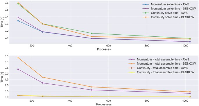
Performance comparison between AWS and Beskow by components, strong scaling
-
Solving the resulting non-linear systems of PDEs by iteratively solving a series of linear systems of PDEs that result from the momentum equation Eq. (1) line (1) and the continuity equation Eq.(1) line (2). The continuity equation requires considerably more iterations to solve, thereby taking more time than the momentum Fig. 10.

In the results below, we analyze these parts of the runtime separately and together to have a better overview. The first plot in Fig. 10 compares the elapsed time for solving the momentum and the continuity equation with 128, 256, 512, and 1024 processes on Beskow and the AWS EC2 cluster.
The second plot in Fig. 10 compares the elapsed time for assembling both the left-hand side and the right-hand side in both environments. The time is plotted on a log scale to be able to represent both functions of different orders in one plot.
The first and second plot in Fig. 11 show the total elapsed time and speedup from 128 to 1024 processes (with one core per processor). The third plot in Fig. 11 shows the relative speedup of the two major components of the runtime, associated with the momentum and the continuity in both environments (with the first datum taken as a reference).

Performance comparison between AWS and Beskow, strong scaling
Table 3 shows the ratio \(\frac{\text {speedup AWS}}{\text {speedup Beskow}}\). In terms of strong scaling, relative to the first datum in Fig. 10 ( for 128 processors), Beskow exhibits slightly better scaling than AWS given that the ratios are less than 100% (Table 3, and the second plot in Fig. 11).
Table 4 quantifies the plots shown in Fig. 10. From it, we can conclude that we get a considerable speedup on the AWS EC2 cluster for the assembly of the system compared to Beskow (see line 2 and line 4 in Table 4). For the momentum, it is up to 1.4 times faster, and for the continuity, it is up to 1.2 times faster on the AWS EC2 cluster. Solving the systems of PDEs using the Stabilized version of BiConjugate Gradient for the momentum and Conjugate Gradient for the continuity (in combination with successive over-relaxation (SOR) preconditioning) results in a very similar performance in both environments. Moreover, we can see that for the momentum, we get a slightly better speedup on AWS, while overall Beskow shows slightly better speedup for the whole application (second plot in Fig. 10). In terms of elapsed time, the CFD application better performance on the AWS EC2 cluster than on Beskow (see Table 4, values over 100% are in favor of AWS).
6.4.2 Strong scaling on AWS EC2 cloud
The application shows very satisfactory scaling on the AWS EC2 cluster for up to 2304 processes with 72 processes per node Fig. 12. Since the size of the problem is more suitable for a smaller number of nodes, we observe an even better scaling for up to 1024 processes with 32 processes per node Fig.

AWS Performance, strong scaling, 72 processes per node

AWS Performance, strong scaling, 32 processes per node
13.
6.4.3 Compute cost comparison
In this section we only look at the cost of the compute time. We highlight that depending on the type of EBS volume chosen, the cost of EBS can add considerably to the total cost.
AWS offers three alternatives for the cluster type that affect the cost of the compute time (see cluster_type in Table 2): on-demand (most reliable, with reservation), spot (use unused EC2 instances for a lower price), dedicated (serving a single customer), and mixed strategies.
Figure 14 shows the fluctuations of the price per hour for the C5n.18xlarge instances in the past year in the us-east region, and all its zones. We have run calculations in the us-east-1a zone - the most stable region. We note that the most volatile zone is us-east-1d with minimum and maximum price of 1.3157$ and 1.5803$ per hour, respectively. Figure 15 shows the savings of on-demand over spot on the 18th of February 2022, with savings from 61.41% to 69.86% for the us-east-1a zone.

Spot pricing for the us-east region for c5n.18xlarge instances in the period March 2021 to March 2022

Current On-demand and Spot pricing for the us-east region for c5n.18xlarge instances
Cost-wise, we observe that the prices for the spot instances are comparable: 0.024€/core-hour on Beskow (a flat rate set by the PDC Center for High-Performance Computing), 0.030€/core-hour for C5n.18xlarge spot instances (based on the average price for zone us-east-1a shown in Fig. 14), and 0.047€/core-hour for dedicated C5n.18xlarge instances, with the exchange rates defined by the European Central Bank (ECB) on the 18th of February 2022. Using this data as reference, the savings over on-demand for the past year for the zone us-east-1a range from 69.8% to 70%.
We report the results from running on the spot nodes. The difference between the spot nodes and the on-demand nodes is in the availability. The spot nodes might become unavailable and interrupt the execution of the program. The availability depends on the current demand and the data center/time zone that we are using. In the reported results, 100% of the runs have been uninterrupted and in fact the frequency of interruption is less than 5% of the time with 70% and up savings over on-demand. For the C5n family, the billing is per hour and choosing between spot and on-demand does not make a difference in the performance because the access to the node does not vary and since it is the largest in the family, in both cases, we were the only tenants (a tenant is a guest on the host machine, a virtual machine) on the node, with exclusive access to all its resources. We chose to use the C5n.x18large instance in the C5n family because it is the largest in the family, which means that whenever we get an allocation we are not sharing with other users. The only difference is that there is a chance that the computation will be interrupted by another tenants if the demand is high when using the spot instances.
Additionally, we have taken all the precautions for ensuring that we are not taking into account any results from interrupted instances by setting up interrupt notices, defining the interruption behavior, using the AWS console tools for finding interrupted instances, checking the billing and finally verification of the validity of the results. Given that we do not run critical applications, we deem that the spot instances are a cost-effective solution for our needs.
Since we look at the price per core hour as the main parameter for optimization, it means, slightly more work is done per hour on AWS than on Beskow (despite the fact that is scales slightly worse than Beskow).
7 Discussion and limitations
The purpose of this paper is to show that there are strong indicators that one can get the very similar performance of HPC applications for the same money on both the supercomputer and the cloud. It is a result of very recent trends and technologies and there is scarce evidence showing this conclusion for tightly-coupled HPC applications.
The final performance depends on a number of factors, which, while we can analyze separately, we have no way of quantifying completely how much they will affect the performance. Therefore we opt not to do an adjustment of the kind of scaling the strong scaling results by the ratio of the compute power of the machines (frequency for example). There are other factors apart from compute power, such as network speed, the impact of RAM memory, storage speed, MPI implementation details and algorithms, MPI tuning, message size, instruction set, types of instructions, turbo boost mode, and other architecture specific characteristics of the hardware, which cannot be directly accounted for with two largely different architectures. The MPI implementation differences, algorithm tuning, and underlying network can potentially have significant impact on the performance. For example, as it can be seen from the MPI benchmarks, the collective algorithms behind the Intel MPI implementation on AWS yield decidedly better performance for the window of message sizes characteristic for our application, while the latency between two processes does not.
Therefore we rely on benchmarks relevant for what we want to test, i.e. run the same code on the machine and look at the effective performance. In this case we incrementally increased the specificity of the benchmarks and finally we ran our application.
7.1 Compute power
The performance of benchmarks such as the NAS EP (Embarrassingly Parallel) benchmark, largely depend on the compute power. The frequency in general does not necessarily scale the same way as performance, because it depends on other factors such as architecture, instructions set, theoretical and sustained number of instructions/sec, theoretical and sustained FLOPS, dynamic frequency, compiler settings, and system processes running in the background. In order to assume this approximation, we have to make a lot of assumptions, for the compute related parameters, as well as otherwise. Given the many differences in the architectures, we opted for relying on benchmarks to examine the most influential indicators of the performance, and finally optimize for cost per hour and maintainability.
7.2 Network
The network performance is one of the most important factors alongside compute power in the HPC world. As the architectures grow more complex, so is the technology improved and occasionally reinvented. However, the fact is that network technology lags behind compute performance advances by large in both on-premise architectures and in cloud environments [37].
The InfiniBand interconnect is one of the most popular ones among supercomputers. The Infinibanch technology stretches from the data layer to the transport layer in the The Open Systems Interconnection model (OSI model [60]). The latency is very low, the bandwidth is very high up to 200Gb/s with HDR links and 100Gb/s with EDR links in the case of Beskow. This interconnect is universal for all traffic types (such as communication between nodes, storage etc). This is made possible by offloading a significant amount of work previously performed in software to hardware, such as the one done by the transport protocol. It also supports bypassing the OS completely to get directly to the physical layer when sending messages across the network, with zero copy, from the application space. This RDMA feature is crucial for capitalizing on the large interconnect bandwidth, given that repeatedly copying the message to be sent incurs time delays due to the limited memory bandwidth. Memory latency and bandwidth improvements have been stretched to a limit in the last years, and innovative technology, such as 3D-stacked DRAM, is on the rise.
The Elastic Fabric Adapter (EFA) is a network device that similarly to the InfiniBand’s RDMA features has the power to bypass the OS to send communications to other instances in the same subnet. The compute nodes in the AWS cluster we have created are placed in the same subnet. The user can configure MPI with the Libfabric framework, the interface between the user space and the kernel space. This framework provides access to the drivers of the EFA network device, making it possible to bypass the OS. AWS has also developed a new transport protocol for their needs, the scalable reliable datagram (SRD) [61]. The SRD focuses on minimizing the traffic congestion and therefore latency for large messages, as well as combating load imbalance (crucial for HPC applications). It sends packages out of order, on various paths with relatively low traffic, to achieve a bandwidth of 100Gb/s. SRD is therefore faster for larger messages, with a high bandwidth overall, and a decidedly improved performance of collective MPI calls. This is in accordance with the findings in the Section 5. Similarly to the transport protocol in InfiniBand, the workings of SRD are offloaded to hardware, the in-house Nitro networking card of AWS.
Cloud providers that offer HPC capabilities use different network and routing protocols, however most of the ones that deliver network bandwidth larger than 100 Gbps rely on RDMA or RDMA-like technologies, omnipresent in on-premise infrastructures [37].
In summary, Beskow has notably lower ping-pong latency for smaller message sizes, however, as the message size increases, in the middle range up to 256 KiB, AWS is on par with Beskow. For the larger message sizes, Beskow is again on top in terms of latency. Both environments have a theoretical bandwidth of 100Gb/s and from the bandwidth benchmarks, we can conclude that the effective bandwidth of AWS exceeds the one of Beskow up to 256KiB. For larger messages sizes, up to 1MiB, Beskow has an edge over AWS. In the 256KiB window of message sizes relevant for our application, Beskow has lower latency, however AWS exhibits higher bandwidth.
7.3 Software maintenance
Comments on cost of maintenance: Spack greatly simplifies the process of deployment in our case. It is an easy way of handling dependencies, and allows for a separate environment, minimizing conflicts with other versions and packages. Installing the FEniCS-HPC stack on a new cluster in general is time-consuming because of the multitude of dependencies and external libraries it makes use of. However, with Spack, the process has been considerably accelerated.
7.4 Overall performance
In terms of compute power, AWS is superior to Beskow, given the more powerful processor and the larger number of cores (Table 1). We have confirmed this with the Open MPI and MPI results for the EP benchmark, part of the NAS Parallel Benchmarks suite. Our application is balanced between compute and memory intensive. Therefore, whereas Beskow has better networking, lower latency for most of the relevant window of message sizes and comparable and superior bandwidth for medium and large message sizes correspondingly, AWS has more compute power.
On the other hand, the MPI communication makes up a large percentage of the application runtime, especially as the number of processes increases. From the benchmarks Section 5, we can clearly see that the elapsed time increases with the number of processors and message size. In the profiling case in Subsection 6.3 with 256 processes on 8 nodes, the MPI communications takes 14% of the runtime. From the profiling and the results of the OSU benchmarks for the most time-consuming MPI functions, we can conclude that on the AWS platform, we get an edge over Beskow, when it comes to MPI communications.
Through the profiling and benchmarking, we have been able to gain an insight into the impact of key factors on the overall performance, as well as the performance of separate components, such as MPI communication, assembly, and solving the resulting systems of equations. Finally, we observe that it is possible to obtain a slightly better performance on the cloud in terms of elapsed time.
8 Conclusion
In this paper, we have shown the results from running the OSU micro-benchmarks relevant for our target HPC application and the NAS Parallel macro-benchmarks in two environments: AWS EC2 cluster and Beskow supercomputer. We conducted a comparative analysis for a wide range of message sizes and processes of the full sets of benchmarks to conclude that our application is suitable to be run in the cloud. The final results show strong scaling up to 2304 cores in the cloud, and the performance is highly competitive with the one on Beskow.
Finally, we have successfully ported a large-scale HPC application to the cloud, providing further evidence of a shift that began in 2020, contrary to an abundance of prior feasibility studies. The performance competes with the one on the supercomputer. Additionally, we get a fully configurable and scalable environment we can tweak for our needs. As a conclusion, this study confirms that due to recent advances, most notably on the networking technologies front, the cloud is getting closer to the on-premise supercomputer, performance-wise, for HPC applications. The increased adoption of cloud within research and furthermore, the most recent advances in network technology by cloud service platforms (AWS, Azure making available network bandwidth of 200 Gbps [62,63,64]) are opening yet again new frontiers for further exploration of the future of HPC.
Data availability
The datasets generated during and/or analysed during the current study are not publicly available due to awaiting publication but are available from the corresponding author on reasonable request.
Notes
The problem sizes of the NAS Parallel Benchmarks from smallest to largest are categorized into classes S, W, A, B, C, D, E, and F. For the CG benchmark, the size of the problem ranges from 1.4K rows in the left-hand side matrix to 54 million rows. Class C packs 150K rows and size D packs 1.5 million rows for CG.
References
Birje, M.N., Challagidad, P.S., Goudar, R., Tapale, M.T.: Cloud computing review: concepts, technology, challenges and security. Int. J. Cloud Comput. 6(1), 32–57 (2017). https://doi.org/10.1504/IJCC.2017.083905
Walker, E.: Benchmarking amazon ec2 for hig-performance scientific computing. ; login:: the magazine of USENIX & SAGE 33(5), 18–23 (2008)
Napper, J., Bientinesi, P.: Can cloud computing reach the top500? In: Proceedings of the Combined Workshops on UnConventional High Performance Computing Workshop Plus Memory Access Workshop, pp. 17–20 (2009). https://doi.org/10.1145/1531666.1531671
Ostermann, S., Iosup, A., Yigitbasi, N., Prodan, R., Fahringer, T., Epema, D.: A performance analysis of ec2 cloud computing services for scientific computing. In: International Conference on Cloud Computing, pp. 115–131 (2009). https://doi.org/10.1007/978-3-642-12636-9_9. Springer
Netto, M.A., Calheiros, R.N., Rodrigues, E.R., Cunha, R.L., Buyya, R.: Hpc cloud for scientific and business applications: Taxonomy, vision, and research challenges. ACM Computing Surveys (CSUR) 51(1), 1–29 (2018). https://doi.org/10.1145/3150224
Arinze, B., Anandarajan, M.: Factors that determine the adoption of cloud computing: A global perspective. Int. J. Enterp. Inf. Syst. 6(4), 55–68 (2010). https://doi.org/10.4018/jeis.2010100104
He, Q., Zhou, S., Kobler, B., Duffy, D., McGlynn, T.: Case study for running hpc applications in public clouds. In: Proceedings of the 19th ACM International Symposium on High Performance Distributed Computing, pp. 395–401 (2010). https://doi.org/10.1145/1851476.1851535
Jackson, K.R., Ramakrishnan, L., Muriki, K., Canon, S., Cholia, S., Shalf, J., Wasserman, H.J., Wright, N.J.: Performance analysis of high performance computing applications on the amazon web services cloud. In: 2010 IEEE Second International Conference on Cloud Computing Technology and Science, pp. 159–168 (2010). https://doi.org/10.1109/CloudCom.2010.69. IEEE
Rehr, J.J., Vila, F.D., Gardner, J.P., Svec, L., Prange, M.: Scientific computing in the cloud. Comput. sci. Eng. 12(3), 34–43 (2010). https://doi.org/10.1109/MCSE.2010.70
Gupta, A., Milojicic, D.: Evaluation of hpc applications on cloud. In: 2011 Sixth Open Cirrus Summit, pp. 22–26 (2011). https://doi.org/10.1109/OCS.2011.10. IEEE
Zhai, Y., Liu, M., Zhai, J., Ma, X., Chen, W.: Cloud versus in-house cluster: evaluating amazon cluster compute instances for running mpi applications. In: State of the Practice Reports, pp. 1–10 (2011)
Coghlan, S.: The magellan final report on cloud computing. Technical report (dec 2011). https://doi.org/10.2172/1076794
Mehrotra, P., Djomehri, J., Heistand, S., Hood, R., Jin, H., Lazanoff, A., Saini, S., Biswas, R.: Performance evaluation of amazon ec2 for nasa hpc applications. In: Proceedings of the 3rd Workshop on Scientific Cloud Computing, pp. 41–50 (2012). https://doi.org/10.1145/2287036.2287045
Expósito, R.R., López Taboada, G., Pardo, X.C., Tourino, J., Doallo Biempica, R.: Running scientific codes on amazon ec2: A performance analysis of five high-end instances. J. Comput. Sci. Technol. 13(3), 153–159 (2013)
Expósito, R.R., Taboada, G.L., Ramos, S., Touriño, J., Doallo, R.: Performance analysis of hpc applications in the cloud. Futur. Gener. Comput. Syst. 29(1), 218–229 (2013). https://doi.org/10.1016/j.future.2012.06.009
Sadooghi, I., Martin, J.H., Li, T., Brandstatter, K., Maheshwari, K., de Lacerda Ruivo, T.P.P., Garzoglio, G., Timm, S., Zhao, Y., Raicu, I.: Understanding the performance and potential of cloud computing for scientific applications. IEEE Transactions on Cloud Computing 5(2), 358–371 (2015). https://doi.org/10.1109/TCC.2015.2404821
Rad, P., Chronopoulos, A., Lama, P., Madduri, P., Loader, C.: Benchmarking bare metal cloud servers for hpc applications. In: 2015 IEEE International Conference on Cloud Computing in Emerging Markets (CCEM), pp. 153–159 (2015). https://doi.org/10.1109/CCEM.2015.13. IEEE
Freniere, C., Pathak, A., Raessi, M., Khanna, G.: The feasibility of amazon’s cloud computing platform for parallel, gpu-accelerated, multiphase-flow simulations. Comput. Sci. Eng. 18(5), 68–77 (2016). https://doi.org/10.1109/MCSE.2016.94
Gupta, A., Faraboschi, P., Gioachin, F., Kale, L.V., Kaufmann, R., Lee, B.-S., March, V., Milojicic, D., Suen, C.H.: Evaluating and improving the performance and scheduling of HPC applications in cloud. IEEE Trans. Cloud Comput. 4(3), 307–321 (2016). https://doi.org/10.1109/TCC.2014.2339858
Ditter, A., Graf, G., Fey, D.: Fe2vcl2: from bare metal to high performance computing on virtual clusters and cloud infrastructure. In: Proceedings of the 4th Workshop on CrossCloud Infrastructures & Platforms, pp. 1–7 (2017)
Balis, B., Figiela, K., Jopek, K., Malawski, M., Pawlik, M.: Porting hpc applications to the cloud: A multi-frontal solver case study. J. Comput. Sci. 18, 106–116 (2017). https://doi.org/10.1016/j.jocs.2016.09.006
Mohammadi, M., Bazhirov, T.: Comparative benchmarking of cloud computing vendors with high performance linpack. In: Proceedings of the 2nd International Conference on High Performance Compilation, Computing and Communications, pp. 1–5 (2018). https://doi.org/10.1145/3195612.3195613
Breuer, A., Cui, Y., Heinecke, A.: Petaflop seismic simulations in the public cloud. In: International Conference on High Performance Computing, pp. 167–185 (2019). https://doi.org/10.1007/978-3-030-20656-7_9. Springer
NASA: NASA SC19 - High-Performance Computing in the Azure Cloud. NASA Technical Reports Server (2023)
Maliszewski, A.M.: Impact of network interconnection in cloud computing environments for high-performance computing applications (2021)
Maliszewski, A.M., Roloff, E., Carreño, E.D., Griebler, D., Gaspary, L.P., Navaux, P.O.A.: performance and cost-aware hpc in clouds: A network interconnection assessment. In: 2020 IEEE Symposium on Computers and Communications (ISCC), pp. 1–6 (2020). https://doi.org/10.1109/ISCC50000.2020.9219554
10 years later: Cloud computing is closing the performance gap. https://doi.org/10.1145/3447545.3451183
Zhuang, J., Jacob, D.J., Lin, H., Lundgren, E.W., Yantosca, R.M., Gaya, J.F., Sulprizio, M.P., Eastham, S.D.: Enabling high-performance cloud computing for earth science modeling on over a thousand cores: Application to the GEOS-chem atmospheric chemistry model. Journal of Advances in Modeling Earth Systems 12(5) (2020). https://doi.org/10.1029/2020ms002064
Panda, D.K., Subramoni, H., Chu, C.-H., Bayatpour, M.: The mvapich project: transforming research into high-performance mpi library for hpc community. J. Comput. Sci. 52, 101208 (2021). https://doi.org/10.1016/j.jocs.2020.101208
Fernandez, A.: Evaluation of the performance of tightly coupled parallel solvers and mpi communications in iaas from the public cloud. IEEE Trans. Cloud Comput. 10(4), 2613–2622 (2022). https://doi.org/10.1109/TCC.2021.3052844
White., Emma.: Running ANSYS Fluent on Amazon EC2 C5n with Elastic Fabric Adapter (EFA). AWS EC2 (2019). https://aws.amazon.com/es/blogs/compute/running-ansys-fluent-on-amazon-ec2-c5n-with-elastic-fabric-adapter-efa/
Appa, J., Turner, M., Ashton, N.: Performance of cpu and gpu hpc architectures for off-design aircraft simulations. In: AIAA Scitech 2021 Forum, p. 0141 (2021). https://doi.org/10.2514/6.2021-0141
Amazon Web Services: AWS HPC. Amazon Web Services (2023). https://aws.amazon.com/hpc/
Azure High-Performance Computing
Google: Google Cloud High-Performance Computing. Google (2023). https://cloud.google.com/solutions/hpc
Chang, Y.-T., Hood, R.T., Jin, H., Heistand, S.W., Cheung, S.H., Djomehri, M.J., Jost, G., Kokron, D.S.: Evaluating the suitability of commercial clouds for nasa’s high performance computing applications: A trade study. Technical report (2018)
De Sensi, D., De Matteis, T., Taranov, K., Di Girolamo, S., Rahn, T., Hoefler, T.: Noise in the clouds: Influence of network performance variability on application scalability. Proceedings of the ACM on Measurement and Analysis of Computing Systems 6(3), 1–27 (2022). https://doi.org/10.48550/arXiv.2210.15315
Intel: HPC Performance Characterization. Intel Corporation (2023). https://www.intel.com/content/www/us/en/docs/vtune-profiler/user-guide/2023-0/hpc-performance-characterization-view.html
Amazon Web Services: AWS Parallel Cluster. Amazon Web Services (2021). https://aws.amazon.com/hpc/parallelcluster/
Amazon Web Services: Elastic Fabric Adapter. Amazon Web Services (2021)
Amazon Web Services: AWS ParallelCluster Documentation. Amazon Web Services (2021). https://docs.aws.amazon.com/parallelcluster/
Barr., Jeff: Now Available - Elastic Fabric Adapter (EFA) for Tightly-Coupled HPC Workloads. Amazon Web Services (2019). https://aws.amazon.com/blogs/aws/now-available-elastic-fabric-adapter-efa-for-tightly-coupled-hpc- workloads/
Amazon Web Services: Amazon EC2 Compute Optimized Instances. Amazon Web Services (2023). https://docs.aws.amazon.com/AWSEC2/latest/UserGuide/compute-optimized-instances.html
Amazon Web Services: Amazon EC2 Instance Types. Amazon Web Services (2023). https://aws.amazon.com/ec2/instance-types/
Amazon Web Services: AWS Nitro System. Amazon Web Services (2021). https://aws.amazon.com/ec2/nitro/
impact of using multi-levels of parallelism on hpc applications performance hosted on azure cloud computing. https://doi.org/10.1504/IJHPCN.2019.098579
Ouro, P., Lopez-Novoa, U., Guest, M.F.: On the performance of a highly-scalable computational fluid dynamics code on amd, arm and intel processor-based hpc systems. Comput. Phys. Commun. 269, 108105 (2021). https://doi.org/10.1016/j.cpc.2021.108105
Gamblin, T., LeGendre, M., Collette, M.R., Lee, G.L., Moody, A., De Supinski, B.R., Futral, S.: The spack package manager: bringing order to hpc software chaos. In: Proceedings of the International Conference for High Performance Computing, Networking, Storage and Analysis, pp. 1–12 (2015). https://doi.org/10.1145/2807591.2807623
AWS: AWS Workshop. AWS (2023). https://catalog.us-east-1.prod.workshops.aws/workshops/dd0ffcb3-ffc1-4b58-8c4b-09f9846549c7/en-US
PDC Center for High Performance Computing: Beskow. PDC Center for High Performance Computing (2021)
Network-Based Computing (NBC) Laboratory, The Ohio State University: MVAPICH: MPI over InfiniBand, Omni-Path, Ethernet/iWARP, and RoCE. Network-Based Computing (NBC) Laboratory, The Ohio State University (2021). https://mvapich.cse.ohio-state.edu/benchmarks/
Lin, H.: Abnormal in-node latency with EFA enabled. Github, aws-parallelcluster (2019). https://github.com/aws/aws-parallelcluster/issues/1143
NASA Advanced Supercomputing (NAS) Division NASA Advanced Supercomputing (NAS) Division (2021). https://www.nas.nasa.gov/publications/npb.html
Hoffman, J., Jansson, J., Jansson, N.: Fenics-hpc: Automated predictive high-performance finite element computing with applications in aerodynamics. In: International Conference on Parallel Processing and Applied Mathematics, pp. 356–365 (2015). https://doi.org/10.1007/978-3-319-32149-3_34. Springer
Jansson, J., Krishnasamy, E., Leoni, M., Jansson, N., Hoffman, J.: Time-resolved adaptive direct fem simulation of high-lift aircraft configurations. In: Numerical Simulation of the Aerodynamics of High-Lift Configurations, pp. 67–92. Springer, ??? (2018). https://doi.org/10.1007/978-3-319-62136-4_5
Jansson, N., Hoffman, J., Nazarov, M.: Adaptive simulation of turbulent flow past a full car model. In: SC’11: Proceedings of 2011 International Conference for High Performance Computing, Networking, Storage and Analysis, pp. 1–8 (2011). IEEE
Hoffman, J., Jansson, J., de Abreu, R.V., Degirmenci, N.C., Jansson, N., Müller, K., Nazarov, M., Spühler, J.H.: Unicorn: parallel adaptive finite element simulation of turbulent flow and fluid-structure interaction for deforming domains and complex geometry. Comput. Fluids 80, 310–319 (2013)
Integrated Performance Monitor (IPM): Integrated Performance Monitor. Integrated Performance Monitor (IPM) (2021). http://ipm-hpc.sourceforge.net/
Jansson, N.: A hybrid mpi+pgas approach to improve strong scalability limits of finite element solvers. In: 2020 IEEE International Conference on Cluster Computing (CLUSTER), pp. 303–313 (2020). IEEE
Kumar, S., Dalal, S., Dixit, V.: The osi model: overview on the seven layers of computer networks. Int. J. Comput. Sci. Inf. Technol. Res. 2(3), 461–466 (2014)
Shalev, L., Ayoub, H., Bshara, N., Sabbag, E.: A cloud-optimized transport protocol for elastic and scalable hpc. IEEE Micro 40(6), 67–73 (2020). https://doi.org/10.1109/MM.2020.3016891
Amazon Web Services: AWS EC2 HPC6i Instance Types. Amazon Web Services (2022). https://aws.amazon.com/es/ec2/instance-types/hpc6i/
Amazon Web Services: New General Purpose, Compute Optimized, and Memory Optimized Amazon EC2 Instances with Higher Packet Processing Performance. Amazon Web Services. https://aws.amazon.com/blogs/aws/new-general-purpose-compute-optimized-and-memory-optimized-amazon-ec2-instances-with-higher-packet-processing-performance/
Azure HBv2-Series Virtual Machines. https://learn.microsoft.com/en-us/azure/virtual-machines/hbv2-series
Acknowledgements
The authors would like to thank Johan Jansson for initiating the idea of exploring the possibilities of the cloud, providing support in obtaining the resources, and the initial mesh for the CFD simulation. This project has received funding from the European Union’s Marie Skłodowska-Curie Actions (MSCA) Innovative Training Network (ITN) H2020-MSCA-ITN-2017 under grant agreement No. 764979.
Funding
Open Access funding provided thanks to the CRUE-CSIC agreement with Springer Nature. This work was supported by the European Union’s Marie Skłodowska-Curie Actions (MSCA) Innovative Training Network (ITN) H2020-MSCA-ITN-2017 under grant agreement No 764979. The authors declare that no funds, grants, or other support were received during the preparation of this manuscript.
Author information
Authors and Affiliations
Contributions
All authors contributed to the study conception and design. The computations and the data analysis were performed by TD. The first draft of the manuscript was written by TD and all authors commented on previous versions of the manuscript. All authors read and approved the final manuscript.
Corresponding author
Ethics declarations
Competing interest
The authors have not disclosed any competing interests.
Additional information
Publisher's Note
Springer Nature remains neutral with regard to jurisdictional claims in published maps and institutional affiliations.
Rights and permissions
Open Access This article is licensed under a Creative Commons Attribution 4.0 International License, which permits use, sharing, adaptation, distribution and reproduction in any medium or format, as long as you give appropriate credit to the original author(s) and the source, provide a link to the Creative Commons licence, and indicate if changes were made. The images or other third party material in this article are included in the article's Creative Commons licence, unless indicated otherwise in a credit line to the material. If material is not included in the article's Creative Commons licence and your intended use is not permitted by statutory regulation or exceeds the permitted use, you will need to obtain permission directly from the copyright holder. To view a copy of this licence, visit http://creativecommons.org/licenses/by/4.0/.
About this article

Cite this article
Dancheva, T., Alonso, U. & Barton, M. Cloud benchmarking and performance analysis of an HPC application in Amazon EC2. Cluster Comput 27, 2273–2290 (2024). https://doi.org/10.1007/s10586-023-04060-4
Received:
Revised:
Accepted:
Published:
Issue Date:
DOI: https://doi.org/10.1007/s10586-023-04060-4