
Abstract
A bespoke ground-motion model has been developed for the prediction of response spectral accelerations, peak ground velocity and significant duration due to induced earthquakes in the Groningen gas field in the Netherlands. For applications to the calculation of risk to the exposed building stock, extensions to the model are required. The use of the geometric mean horizontal component in the ground-motion predictions and the arbitrary horizontal component for the building fragility functions requires the addition of component-to-component variability. A model for this variability has been developed that both reflects the strong horizontal polarisation of motions observed in many Groningen records obtained at short distances and the fact that the strong polarisation is unlikely to persist at larger magnitudes. The other extension of the model is the spatial correlation of ground motions for the calculation of aggregated risk, which can be approximated through simple rules for sampling the variance within site response zones. Making use of ground-motion recordings from several networks in the field and the results of finite difference waveform simulations, a Groningen-specific spatial correlation model has been developed. The new model also combines results from traditional variogram fitting approaches with a new method to infer spatial correlation lengths from observed variance reduction. The development of the new spatial correlation model relaxes the need to approximate spatial correlation through the sampling of site response, although the results obtained herein suggest that similar results could be obtained using either approach. The preliminary consideration of the numerical waveform modelling results in this study paves the way for significant extensions to be made for the modelling of spatial correlations and the decomposition of apparent spatial variability into systematic and random components within a fully non-ergodic framework .
1 Introduction
Gas production in the Groningen field in the northern Netherlands is inducing earthquakes, the largest of which occurred in August 2012 near the village of Huizinge with a magnitude of ML 3.6. A key element in quantifying the consequent hazard and risk due to these induced earthquakes is a model for the estimation of the ground shaking at the surface (van Elk et al. 2017). The earthquakes initiate inside the gas-bearing Rotliegend sandstone layer encountered at a depth of about 3 km and the radiated energy then propagates through the overlying high-velocity Zechstein salt layer, which causes reflections and refractions of the waves (Kraaijpoel and Dost 2013). Overlying the Zechstein is a chalk layer and near the surface there are thick layers of soft soils, including clays, sands and peats, which can be expected to respond non-linearly under stronger levels of shaking.
In view of the unique characteristics of the Groningen earthquakes and the velocity profile between the reservoir and the ground surface, there is a clear need to derive a field-specific ground-motion model. The initial model was based on simulations using source, path and site parameters obtained from inversions of the Fourier amplitude spectra of the recorded motions (Bommer et al. 2016). In the simulations, alternative values of the Brune stress parameter were used in a logic-tree formulation in order to represent epistemic uncertainty associated with the extrapolations from the magnitude range of the data (ML 2.5–3.6) to the largest magnitudes consider in the hazard and risk modelling, which extends to an upper limit of ~ 7.5 (see Bommer and van Elk 2017). In passing we note that for magnitudes ≥ 2.5, moment and local magnitudes in the Groningen field are, on average, equivalent (Dost et al. 2018).
Subsequent developments of the Groningen ground-motion model (GMM) focused on incorporation of local site effects by predicting motions at a reference rock horizon (the base of the North Sea formation, which is at about 800 m depth) and combining these with non-linear frequency-dependent amplification factors (Bommer et al. 2017a). Using a field-wide shear-wave velocity model from the surface to 800 m depth (Kruiver et al. 2017), the field was divided into 160 zones each with non-linear amplification factors for spectral accelerations at 23 response periods and for peak ground velocity (Rodriguez-Marek et al. 2017). The linear portion of the amplification factors for short oscillator periods were found to depend on both magnitude and distance (Stafford et al. 2017). Another enhancement of the GMM development was to move from point-source to extended-rupture simulations (Bommer et al. 2017b; Edwards et al. 2018).
For generation of seismic hazard maps and uniform hazard spectra for the field, the model as described is sufficient. However, for the calculation of potential structural damage to the exposed Groningen building stock, and consequent injuries and fatalities, additional elements of the GMM are required. For some structural types, the fragility is defined not only as a function of spectral acceleration but also of duration (Crowley et al. 2017). Consequently, the GMM also predicts the significant duration of shaking (Bommer et al. 2017a, b) and the model of Bradley (2011) for the correlation of residuals of spectral acceleration and duration is adopted. Since multiple building typologies can be encountered within any of the grid squares in the risk modelling, and since several building types have different fundamental vibration periods in the two orthogonal axes, period-to-period correlations are also required, for which the model of Baker and Jayaram (2008) was adopted. The Groningen ground-motion database is not sufficient to allow the derivation of inter-intensity measure correlation models applicable across the magnitude range considered in the hazard and risk calculations, but local data was used to confirm the applicability of the adopted models.
In this paper, we address two other extensions to the GMM required for the risk calculations, namely the component-to-component variability and a model for the spatial correlation of ground motions. These are presented in the following sections of the paper, which concludes with a discussion of potential refinements of both of these elements within the framework of a transition to a fully non-ergodic model of spatially- and azimuthally-varying predictions of ground motions.
2 Ground-motion database
A large number of recording stations have been installed in the field as part of a series of different networks and recording campaigns in the years since the Huizinge earthquake. The overall database utilised in the present study contains records specifically from the following networks:
-
The KNMI B-network, which consists of 17 accelerographs located mainly, but not exclusively, in the north of the field (Dost et al. 2017).
-
The surface accelerographs only of the KNMI G-network, a network of ~ 80 borehole arrays with an accelerograph at surface level and four geophones at depth intervals of 50 metres; operation of the first stations started in early 2015 (Dost et al. 2017).
-
The TNO-operated household network, consisting of more than 350 accelerographs installed since 2014 within buildings, mainly private residences and a few public buildings. There are concerns that the records obtained from accelerographs of this network that are installed above ground level are contaminated with structural response. Therefore, only records from accelerographs located in basements and crawl spaces below the ground floor are being used until the ongoing investigation of this matter is completed. The accelerographs were installed with a triggering level of 0.1 cm/s PGV, which censored the datasets from earthquakes prior to 2016, when a system to bypass the threshold in case of an earthquake was introduced.
-
The NAM flexible network, a total of 450 geophones, used for passive monitoring since the beginning of 2017, and re-installed at a different location in the field every 2 months, remaining operational for 45 days each time. The flexible network was operational during the latest two earthquakes of ML ≥ 2.5 that occurred in May 2017 and January 2018 (Fig. 1). The geophones of the flexible network have a sampling rate of 250 Hz, identical to the accelerographs of the household network and higher than the accelerographs of the KNMI networks, whose sampling rate is 200 Hz. Their lowest usable frequency was found during signal processing to be in the range 0.5–0.9 Hz.
Fig. 1 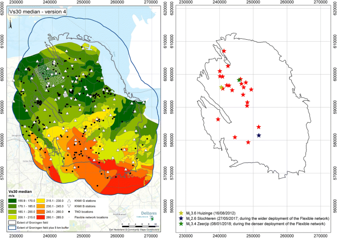
Left: Recording stations, site amplification zones and median VS30 values in the Groningen hazard and risk study region (field boundary plus 5 km buffer); Right: locations of the epicentres of the 24 earthquakes of ML 2.5–3.6 in the Groningen field, highlighting the largest event and the two events recorded on the flexible network array of geophones (grey dots in left-hand plot). Coordinates are in metres in the Dutch RD system

A fifth network is also operational in the field, consisting of the accelerographs installed in the NAM facilities as part of their safe shutdown system. The records it has produced have not been included in this database, as investigation of their usability for model development is still ongoing.
The locations of the epicentres, as well as the locations of the stations which generated these records, are shown in Fig. 1, along with the 160 site amplification zones of the field and the median VS30 value in each zone.
However, the datasets used for the development of the component-to-component variability model, and for the spatial correlation model differ through the use of different subsets of the data shown in Fig. 1. The use of different datasets reflects differences in the development history of these two models. The component-to-component model has been developed in parallel with the ground-motion model used for risk computations in the field to date and so has adopted the same empirical dataset (of just the B and G stations) used for the overall hazard and risk model (Bommer et al. 2018). The more recent availability of the Household and Flexible network records has since enabled consideration of a field-specific spatial correlation model and explains why the extended database is used for the spatial correlation model.
The ground-motion database used for the derivation of the spatial correlation model consists of 1546 records obtained during the 24 earthquakes of magnitudes (ML) between 2.5 and 3.6 that have occurred since 2006 in the Groningen field. For the component-to-component model, only the records from the KNMI B-stations (151 records) and KNMI G-stations (107 records) were used; these were obtained in 23 events since the model was derived before the most recent earthquake included in the spatial correlation database.
Figure 2 shows the accumulation of usable records over time. The installation of extensive networks after 2014, the removal of the PGV-trigger threshold in the household network instruments in 2016, and the deployment of the flexible network have all led to great increases in the number of records obtained from each earthquake. Some 75% of the current database were obtained during the two most recent earthquakes. Figure 3 shows the magnitude-distance distribution of the dataset.

Accumulation of ground-motion records included in this database with time and breakdown of records by network

Magnitude-distance distribution of the ground-motion database
3 Component-to-component variability
Consistent with most modern ground-motion prediction equations (GMPEs) the Groningen GMM predicts the geometric mean values of the horizontal components. However, the structural analyses performed for the derivation of the fragility functions for the exposed building stock make use of single horizontal components of recorded accelerograms. Consequently, the ground-motion predictions need to be converted from the geometric mean to the arbitrary horizontal component for the risk computations. The predicted median values of these two horizontal component definitions are equivalent, but the standard deviation of the geometric mean component needs to be increased to reflect the component-to-component variability (Baker and Cornell 2006).
Within the risk model we define the logarithmic motions at a given point on the surface as:
with \(\mu (\varvec{x},{\mathbf{M}})\) being the log-mean surface motion (which in Groningen is a log-mean reference motion at the base of the north sea formation, NS-B, for magnitude \({\mathbf{M}}\), plus the mean logarithmic site amplification for the given zone), \(\delta_{B}\) being the between-event residual (independent of position), and \(\delta_{{W_{es} }} (\varvec{x})\), \(\delta_{c2c} (\varvec{x})\) and \(\delta_{S2S} (\varvec{x})\) corresponding to the site and event corrected residual at NS-B, the component-to-component residual, and the site amplification residual, all of which can depend upon position \(\varvec{x}\). The variances of these position-dependent components are \(\phi_{SS}^{2}\), \(\sigma_{c2c}^{2}\) and \(\phi_{S2S}^{2}\). Note that this formulation assumes that the site response is linear, but that this assumption does not strongly influence the present treatment. In the present section our focus is upon the development of a model for \(\sigma_{c2c}^{2}\) that describes the variance between the logarithmic amplitudes of the two horizontal components, relative to the geometric mean amplitude.
Ground-motion recordings in Groningen are often seen to be strongly polarised, with inter-component spectral ratios of as much as three or higher across the entire frequency range (Fig. 4). Boore (2005) defined the component-to-component variance of a database as the arithmetic mean of the squares of the component-to-component residuals of the records of that database, as shown in Eq. (2), where N is the number of records and Yij is the ith component from the jth record.

Ordinates of the 5%-damped acceleration response spectrum of two horizontal components of a polarised recording from Groningen (the 2017 ML 2.6 Slochteren earthquake recorded at the G460 station); the solid black curve is the geometric mean of the two component ordinates
Consequently, values of component-to-component variability calculated from the Groningen ground-motion data are much higher than values typically presented for earthquake ground motion (e.g., Boore 2005; Campbell and Bozorgnia 2007). However, when only smaller (M < 6) earthquakes are considered and recordings are limited to short source-to-site distances, higher component-to-component variances are also found within tectonic databases, but the variability remains smaller than that found for Groningen (Bommer et al. 2017a). The more extensive database for Groningen now available shows that the component-to-component variance is distance-dependent, consistent with the observation that strongly polarised motions are generally recorded close to the earthquake epicentres. This distance- and magnitude-dependence is interpreted as indicating that the polarisation is due to the shear-wave radiation pattern from the shallow sources of the small-magnitude earthquakes in Groningen. At greater distances, the interaction of direct and indirect phases will diminish the polarisation. For larger earthquakes, the interaction of radiation patterns from adjacent segments of the fault rupture would break down the polarisation in a similar manner.
A model for the component-to-component variance has been constructed to reflect the observed distance dependence and inferred magnitude dependence. Firstly, a simple function is fit to the variance values to capture the dependence on distance, and this model is assumed to hold in the magnitude range of the data (ML 2.5–3.6). Secondly, it is assumed that at larger magnitudes the component-to-component variance would be comparable to that from tectonic models, for which we adopt Campbell and Bozorgnia (2007); a simple linear transition from Groningen-specific to typical tectonic values is assumed over two magnitude units (Fig. 5).

Magnitude- and distance-dependent model for component-to-component variability for the 0.1-s spectral acceleration together with the Groningen database component-to-component residuals, grouped by rupture distance: < 5.5 km (red), 5.5–15 km (blue) and > 15 km (green). The vertical axis shows \(\delta_{c2c}\) for individual records, and \(\sigma_{c2c}\) for the plotted model
The variance values at different periods are found to be well represented by a trilinear function with constant values below 0.1 and above 0.85 s. The model for the component-to-component variance of duration is constructed in a similar manner but converging at larger magnitudes to the values proposed by Bommer et al. (2009) for tectonic earthquakes.
The component-to-component variance in the model presented is defined by the following equations for different periods, rupture distances and magnitudes, T, R and M:
For periods in between 0.1 and 0.85 s, the following interpolation is used:
4 Model for spatial correlation
In response to regulatory requirements in the Netherlands, the primary metric in the Groningen risk calculations is Local Personal Risk, which is specific to individual locations (Crowley et al. 2017). For any spatially-aggregated risk metric, such as Group Risk, spatial correlation in the ground-motion field is necessary to avoid underestimation of the risk. The efforts to address this potential need are presented in this section, starting with a summary of how spatial correlation is currently approximated in the current risk calculations. The remainder of the section presents the derivation of a new Groningen-specific spatial correlation model, starting with a summary of the empirical data used and waveform simulations to model spatial correlation.
4.1 Simplified model in current risk calculations
The ground-motion model used for hazard and risk calculations in the Groningen field combines field-specific predictions of motions at a reference velocity horizon, approximately 800 m below the ground surface at the base of the North Sea formation (the NS-B horizon), with near surface site response effects. Within a Monte Carlo framework, reference motions are first generated for this horizon before these motions are modified to account for local site effects using zone-specific site amplification functions for each of the 160 zones. One of the ultimate goals of the project is to develop spatial correlation models that consistently account for correlations within the paths leading to the NS-B horizon, and to then appropriately reflect spatial correlations within the site response.
For the current risk calculations the overall field is discretised into spatial cells that are represented by a ‘grid point’. The typical spatial separation of these grid points is 500 m. The site response model for the field is also discretised into 160 separate ‘zones’. These zones were previously shown in Fig. 1 and while their geometries vary significantly, it is possible to determine a representative spatial scale for each zone \(z\) as follows:
That is, we compute the area, \(A_{z}\), of each zone and then compute a length scale corresponding to a circular area. Call this the effective zone radius \(r_{{{\text{eff}},z}}\). When these effective zone radii are computed for all zones we obtained the distribution shown in Fig. 6. As can be appreciated from the difference in the typical grid separation distance and the effective zone radii, many zones contain multiple grid points.

Distribution of effective zone radii, \(r_{{{\text{eff}},z}}\), for all 160 site amplification zones in the Groningen field. The total area covered by these site zones is 1409 km2
The overall spatial correlation should ideally be decomposed into components that reflect the partitioning of the overall variability shown in Eq. (1). If these correlation components existed, then the overall spatial correlation can be described by Eq. (6).
Currently, there is no way to constrain the various correlation components in Eq. 6, but a level of spatial correlation is implied by making assumptions about the various components.
Three different options were considered to approximately account for spatial correlation in the existing hazard and risk model. In all cases it is assumed that we have \(\rho_{S2S,ij} = 1\) for two points inside a given site amplification zone. This does not mean that the site response itself is identical throughout a zone because each zone may contain multiple grid points at which hazard calculations are made. Each grid point will therefore have a different source-to-site distance and nonlinear site effects will hence differ from grid point to grid point. However, the variability for grid points within the same zone is perfectly correlated. For grid points in different zones \(\rho_{S2S,ij} = 0\). The three variants that were then considered were:
-
1.
\(\rho_{SS} = 1\) and \(\rho_{c2c} = 1\) throughout a site amplification zone. Combined with the \(\rho_{S2S,ij} = 1\) assumption above, the overall correlation is 1.0 for all points within the same zone, and 0.0 otherwise.
-
2.
\(\rho_{SS} = 1\) and \(\rho_{c2c} = 1\) within any given grid cell, but \(\rho_{SS} = 0\) and \(\rho_{c2c} = 1\) for other grid points within the same site amplification zone.
-
3.
\(\rho_{SS} = 1\) and \(\rho_{c2c} = 0\) within any given grid cell, but \(\rho_{SS} = 0\) and \(\rho_{c2c} = 0\) for other grid points within the same site amplification zone.
The implied correlation for each of these options was compared with the predictions of the Jayaram and Baker (2009) model as well as preliminary regressions on the Groningen database used for the development of the V5 ground-motion model (Bommer et al. 2018). As the component-to-component variability is magnitude and distance dependent, the implied correlation varies with earthquake scenario. Additionally, as all variance components change with period the implied correlation is also period dependent. Figure 7 therefore shows just one example of the implied correlations for each of the three cases for one magnitude-distance scenario. For the purposes of this comparison, site amplification zones are conceptually thought of as being regular cells such that the distance from the centroid shown in Fig. 7 can be related to \(r_{{{\text{eff}},z}}\).

Implied spatial correlation associated with assumptions on the components of Eq. (3). Panels from left to right represent options (1)–(3) described in the text. Each thin grey line represents the correlation for a given site amplification zone. Red lines show variants of the Jayaram and Baker (2009) model—JB (2009). Results are shown for T = 0.01 s, M3, and Rrup = 10 km
From consideration of these implied correlations it was decided to utilise approach (i) of perfect correlation within each site amplification zone as an interim measure ahead of the current study that explicitly develops an initial Groningen-specific model. This approach consciously over-estimates the correlation for closely-spaced sites (over a length scale that depends upon the size of the site zone), but then has zero correlation among sites within adjacent zones.
4.2 Results from waveform simulations
While the empirical dataset compiled to date is very rich for some events, it is still too sparse to provide insights into how correlations are partitioned among the travel path and site response. However, as discussed by Edwards et al. (2018), a number of seismological simulations have been performed for the field. The primary objective of these simulations has been to constrain source and path scaling effects thus far, they can also provide insight into the decomposition of spatial correlation. One of the unique aspects of the Groningen region is the wealth of subsurface information that has been collected over 40 years of exploration and production. This information has allowed the development of a high-quality 3D velocity model for the region which potentially enables systematic path effects to be captured. By using elastic finite difference approaches and detailed 3D elastic models the wave-field can be simulated from the source to a reference rock horizon (Edwards et al. 2018). Such wave fields can then be inspected to understand how the local geology influences the path effects and, in turn, the spatial correlation. This type of modelling has the added advantage in that the wave field can be measured at any given location in the model domain and on a spatially dense grid of receivers.
A key challenge within deterministic modelling of ground motions is the lack of control over the source representation and accurately accounting for how the source complexity scales with magnitude. The kinematics of the source also influence the observed spatial correlations within the field, just as they can effect the component-to-component variability discussed earlier. For the purposes of this study the general slip characteristics, slip, dip and rake, are defined from pre-existing fault architecture and first motions of recorded earthquake data. However, no a priori knowledge of how the internal variability of the fault rupture is assumed, rather a stochastic approach is used to capture variability in the amount of slip, rise time, rupture velocity and direction (Graves and Pitarka 2016). This approach allows us to explore a range of possible fault slip scenarios, to isolate the components of spatial correlation that can be contributed by the systematic path and source effects.
The finite difference simulations used here make use of a detailed 3D elastic model that is derived from well information and high-resolution 3D reflection seismic surveys and was supplied by the field operator, Nederlandse Aardolie Maatschappij (NAM). To model the wave-field that incorporates frequencies of interest (< 30 Hz) and to avoid numerical dispersion the model is defined on a 6.25 m grid. The model dimensions are 40 km × 35 km × 5 km. Synthetic 3-component seismograms are output on a 25 m × 25 m grid. The synthetic receivers are located on a virtual bedrock surface just below the ground surface. Non-linear near surface effects associated with near surface soil conditions are not considered in this part of the study. Synthetic data are recorded for 13 s following event initiation and this enables the peak response at each location to be captured. Further details of these simulations can be found in Edwards et al. (2018).
Multiple rupture scenarios, ranging in magnitude from M 3 to 6, are tested. Examples of the spatial distribution of ground motions arising from these simulations are shown in the upper row of Fig. 8 in terms of logarithmic PGA. All the scenarios make use of non-uniform finite fault surface, where the rate of slip, amount of slip, rise time and rake are allowed to vary through a stochastic approach. Also tested are the impacts of fault aspect ratio and stress drop. Held constant is the fault plane defined by the strike, dip and rake of the rupture, these values are defined to the general trend that is observed in the field (a strike of 270°, dip of 70°, and a rake of 90°).

Examples of simulated peak ground accelerations used in this study as measured on a virtual bedrock surface for magnitudes from left-to-right of M 3, 5 and 6. Coordinates are kilometre versions of the Dutch RD system. The upper row shows logarithmic ground-motions, with warmer colours representing larger motions. The lower panel shows ground-motion residuals with blue and red representing negative and positive residuals. In the lower panel, white indicates the zero level
Figure 8 also shows the ground-motion residuals for the three simulation examples shown. In order to compute these residuals, it is first necessary to define the average attenuation of motions with distance over the simulated field. For this purpose, a trilinear (in log–log space) geometric spreading function was fitted to each set of simulations. For the three examples shown in Fig. 8, the corresponding distance decay is shown in Fig. 9 along with the fitted models in each case. For the small magnitude simulations there is a pronounced change in the geometric spreading that is evident in both Figs. 8 and 9, and this is a known local feature of the Groningen field. The distributions of residuals in the lower row of Fig. 8 shows clear spatial clustering, and an ongoing objective of this work is to understand the difference between systematic and random features of these spatial patterns.

Examples of the average distance dependence of simulated motions for each of the three examples shown in Fig. 8. The colour of each hexagon indicates the density of points at that location, with lighter colours denoting larger counts. The green lines are generalized additive models fit to identify local trends in the data, while the thick red linear are three-branch piecewise linear fits to the data in log–log space
To infer the spatial correlation from the residual fields shown in Fig. 8, semi-variograms are computed using the classical method of moments according to Eq. (7) (Cressie 1993).
In this equation, \(N_{h}\) represents the number of pairs of normalized residuals, \(\varepsilon_{W}\), that are separated by a distance \(h\) to within a tolerance defined by a bin of width \(\Delta h = 0.25\) km. The normalized residuals are computed as \(\varepsilon_{W} = \delta_{W} /\phi\), where \(\delta_{W}\) is the residual computed with respect to the fitted models in Fig. 9, and \(\phi\) is the overall standard deviation of the within-event residuals. Note that here when referring to within-event residuals, these are really within-simulation residuals.
The simulated ground-motion fields shown in Fig. 8 represent 169,015 spatial locations, which is far more than necessary to constrain a macro spatial correlation model. Therefore, for the purposes of computing the semi-variograms according to Eq. (7), a random sample of 10,000 points was first taken from each simulated field. While this is a significant reduction, it still leads to an average value of \(N_{h}\) of well over 300,000 across the considered separation distances and so the variance estimates are extremely well-constrained.
To develop the correlation model from the waveform simulations, 10 scenarios were used (2 at M3, and 4 at each of M5 and 6). The computed semi-variograms for each of these cases are shown in Fig. 10, along with fits to each simulation, and an average fit across all simulations at each magnitude level. To fit the semi-variograms, the loss function of Cressie (1985), as shown in Eq. (8), was minimised in an effort to optimise the fit of the correlation model to high-levels of correlation (low levels of semi-variance).

Variability in spatial correlation resulting from different source representations for three different magnitude ranges (left) M 3, (centre) M 5 and (right) M 6. The magnitude 3 scenario has two different realizations where the fault size and stress drop are held constant. The magnitude 5 event has 4 scenarios of source variability where the size of the rupture was held constant, but the stress drop was allowed to vary from 1.2 to 3.0 MPa. The magnitude 6 also had 4 realizations where the stress drop was held constant, but the aspect ratio of the fault surface was allowed to vary from 2:1 to 6:1. Black circles show the average semi-variance over the simulations, and the thick blue lines are the optimal fits to these averages
In Eq. (8), \(\widehat{\gamma }_{k}\) is the estimated semi-variance, from Eq. (7), in bin \(k\) (associated with separation distance \(h\)), \(n_{k}\) is the number residual pairs in this bin, and \(\gamma_{k} \left( \theta \right)\) is the model semivariogram. The scaling of the semi-variograms strongly suggest that an exponential correlation model is appropriate and so the corresponding model semi-variogram is:
From this formulation, the spatial correlation model can be defined by:
and we note that when normalised residuals are used such that \(\phi^{2} = 1\), the relation between the semi-variance and the correlation is simply \(\gamma \left( {h;\varvec{\theta}} \right) = 1 - \rho (h;r_{c} )\).
The goal of having multiple simulations for each magnitude level is to reduce the uncertainty in the defined spatial correlation that would result from variability in the source kinematics. Figure 10 illustrates the variability in spatial correlation that can be attributed to variability in rupture process while keeping the magnitude fixed for three different cases: M3, M5 and M6. These results illustrate that there is a slight magnitude dependence and a non-trivial contribution from fault rupture process (note that the correlation length, rather than the fluctuations in the semi-variance is the key feature of consideration in this context). The average of the variograms across the three magnitude levels leads to an overall semi-variance very close to the results for the M5 case. This is shown by plotting the actual correlation models obtained from the semi-variograms in Fig. 11.

Average correlation across all 10 simulations (black circles) along with the associated fit (blue thick line). Averages by magnitude are shown using the grey markers and lines. Red lines show the model of Jayaram and Baker (2009) for unclustered (solid) and clustered (dashed) sites
Although only the current results for PGA are shown here, further development of this work will look to test assumptions of isotropy and magnitude-dependence, among other things. For the current stage of development of the overall hazard model it remains necessary to rely primarily upon more conventional empirical approaches. Current efforts in this direction are discussed in the following section.
4.3 Groningen-specific spatial correlation model
The dataset described in Sect. 2 differs considerably from that used for the development of the V5 ground-motion model (Bommer et al. 2018) through the edition of the recordings from both the Flexible array and the Household network. As shown in Table 1 and Figs. 2 and 3, these additional records make a significant difference to the overall number of available records. However, the temporal and spatial distribution of these recordings also poses challenges for the development of a generic spatial correlation model for the field.
Spatial correlation models focus upon correlations among computed within-event residuals, \(\delta_{W} \left( \varvec{x} \right)\), where these residuals are computed with respect to some pre-existing ground motion model, \(\mu (\varvec{x},{\mathbf{M}})\), and an event-specific deviation from this generic model, \(\delta_{B}\) (the between event residual). This formulation is described by Eq. (11).
In the present case, the obvious candidate for the ground-motion model is the current V5 model developed for the Groningen field. However, this model is designed to predict motions for a very broad magnitude range and does not target optimal performance in the narrow magnitude range for which data exist. When the new Household and Flexible network observations are added to the database used within the derivation of the V5 model, it is expected that some bias, \(\beta\), should exist such that the event-specific prediction is really \(\mu \left( {\varvec{x},{\mathbf{M}}} \right) + \beta + \delta_{B}\) at each spatial location \(\varvec{x}\). The first step in the derivation of an empirical spatial correlation model is therefore to define this event-specific prediction and to determine the overall bias and the between-event residual (or random effect) for each earthquake.
In the present study, it is not appropriate to simply perform a random effects regression on the total residuals as is commonly done in other studies (e.g., Jayaram and Baker 2009; Foulser-Piggott and Stafford 2011). The primary reason for this is that the high-density spatial sampling of the Flexible network has a strong influence upon computed random effects. This can be appreciated in Fig. 12 in which random effects for each event are computed using the entire dataset available, just the KNMI-B and KNMI-G stations (used for the calibration of the current ground motion model), and all data with the exception of the Flexible network (FN in Fig. 12). Estimates of the random effects differ from earlier events that are not recorded by the Household or Flexible networks because these new records change the overall bias of the model in each case. What is most evident, however, are the large differences between random effects computed for the most recent events. For events 23 and 24 the random effects for the full dataset are close to zero and this simply reflects the strong weight that the 809 records from the Flexible network have on defining the overall model bias.

Influence of dataset used upon the estimate of between-event residuals (random effects). Errors bars represent the 95% confidence intervals in the estimates of the random effects
However, it is not simply the imbalance in the numbers of records that is problematic, the spatial distribution of the Flexible array also causes issues. When the Flexible network is excluded from the database, the mean inter-station spacing is 14.7 km (about three times the value of \(r_{C}\) for PGA implied by the waveform simulations). However, for the Flexible network the mean inter-station spacing for event 23 is 3.7 km and only 0.5 km for the dense deployment that recorded event 24. Given that we expect spatial correlation to exist in the data, the inclusion of the Flexible network records biases both the random effects and the overall variance, as correlated motions over some spatially-limited cell have lower variance than the overall variance of the field (Stafford 2012).
The process adopted for the development of the generic spatial correlation model for the Groningen field is therefore based upon the following steps:
-
Random effects for each event are computed by excluding the records from the Flexible network. As the mean inter-station spacing for this subset of the data is much larger than the correlation length implied from the waveform simulation results, as well as from previous empirical regression analyses, the random effects should not be strongly influenced by spatial correlation effects (Jayaram and Baker 2010; Stafford 2012).
-
Use the random effects from the previous step to compute within-event residuals for all records (both including and excluding the Flexible network).
-
Investigate the impact of the Flexible network upon the computed semi-variograms, and also constrain the final correlation model through consideration of the variance of within-event residuals over the Flexible array.
Regarding the final step, the high spatial density of the Flexible array, as well as its geometric layout, provides a unique opportunity to constrain spatial correlations in a new manner. Stafford (2012), building upon the work of Vanmarke (1983), explained that the variance of a correlated random field over some finite region, \(A\), is lower than the overall variance of the field. This is shown generically in Eq. (12):
where, \(\phi_{A}^{2}\) is the variance over the spatial region, \(\phi^{2}\) is the overall variance of the spatial field, and \(\psi (\varvec{x};r_{c} )\) is the variance reduction function that depends upon the nature of the spatial correlation within the field. This variance reduction function is defined by Eq. (10), and is equivalent to one minus the average correlation over the region in question:
Events 23 and 24 provide large numbers of observations from the Flexible array over small spatial regions (with different areas in each). These regions are represented by the vector of instrument locations \(\varvec{x}\). The ratio of the variance of \(\delta_{W} (\varvec{x})\) values over these regions to the overall within-event variance therefore gives an empirical estimate of \(\widehat{\psi }(\varvec{x};r_{c} )\) for each event. As the correlations within the field appear well represented by an exponential model of the form shown in Eq. (10), the value of \(r_{c}\) that best matches the computed \(\widehat{\psi }(\varvec{x};r_{c} )\) provides an estimate of the correlation model.
For each response period empirical variograms were computed and exponential correlation models (with and without nugget effects) were fitted to the variograms. Variograms may have nugget effects when the semi-variance for a separation distance of zero is not equal to the theoretically expected value of zero; they manifest as an ‘intercept’ for the variogram. Such effects are typically attributed to measurement uncertainty and could be reflected in the present study by different ground-motion levels for co-located (or very closely spaced) instruments. However, the nugget levels encountered are rather strong here and it is not currently clear what the precise cause of this effect is. That said, the dependence of the nugget strength on the dataset selected suggests that instrument effects are contributing. Figure 13 shows the results from a selection of such computations for a broad range of periods. Empirical and fitted variograms were obtained for different datasets (either including all of the available data, or otherwise excluding records within the Flexible network). The variograms were either fitted using the loss function of Eq. (8) (referred to as ‘Cressie’), or a simplified version of this expression that does not include the denominator of \(\gamma_{k} \left(\varvec{\theta}\right)\) (referred to as ‘npairs’). The exponential models were also fit with and without consideration of a nugget effect.

Comparison of empirical and fitted semi-variograms for different datasets and model fitting approaches. Line types indicate whether or not a nugget effect was considered. Colours represent combinations of datasets (either ‘All’ data being used, or ‘NF’ for ‘Not Flexible network’) and loss functions used for the fitting (either Cressie’s variance weighted fit, or fits weighted by numbers of pairs of observations at each separation distance)
Figure 13 shows that there is a significant difference between the empirical variograms obtained with and without consideration of the Flexible network data. In particular, when the Flexible network data is excluded the data exhibits a very strong nugget effect. Such nugget effects are typically associated with measurement uncertainty, but in this particular case it appears likely that at least part of this effect is reflecting differing levels of inherent variability among the types of instruments that have been deployed throughout the field. At this point, as can be seen from Table 1, there is too little overlap among sets of records obtained from each instrument type to resolve this issue. However, it is certainly a matter for further consideration.
Figure 14 summarises the correlation lengths that are implied by each combination of dataset and fit. There is a significant spread of correlation lengths depending upon the approach employed, and it should be noted that all results shown in Fig. 14 correspond to cases in which a nugget effect is included. The variation is even greater when the nugget is forced to zero (equivalent to having no nugget effect). In Fig. 14 the results obtained from optimising the variance reduction function of Eq. (10) are shown along with the more traditional variogram fitting methods. The results for Event 23 suggest significantly greater correlation lengths than is the case for Event 24. However, it is interesting to note that the Flexible network for Event 23 covered approximately 50 km2 and spanned multiple site amplification zones while Event 24 covered just 1 km2 and was contained entirely within a single zone. The solid and dashed lines in Fig. 14 represent the Jayaram and Baker (2009) correlation model for cases where site conditions exhibit clustering or otherwise. The variance reduction function results for the larger area are more consistent with the clustered site condition results from Jayaram and Baker (2009), while the Event 24 results are far more consistent with the unclustered case.

Correlation lengths implied by all considered combinations of dataset and fitting approach. The grey lines represent the model of Jayaram and Baker (2009) for clustered (dashed) and unclustered (solid) site conditions. Colours represent the dataset used (‘All’ is for the entire dataset, ‘NF’ is ‘Not Flexible network’ and ‘FN-EXX’ is the Flexible network data used for Event XX along with the variance reduction approach). Marker shapes denote fitting type with the approaches of Fig. 13 complimented here by the variance reduction approach as well
In Fig. 13 it is apparent for response periods of 0.3 and 0.5 s that the empirical variograms have not reached a stable plateau at 20 km separation distance. In the fitting process there is a trade-off between the sill, or partial sill, level and the correlation length, and around these intermediate response periods the relatively long correlation lengths shown in Fig. 14 are partially biased as a result of these total sill levels being too high. To generate Fig. 13 the within-event residuals have been normalised and so there is an expectation that the total sill should be very close to unity for large separation distances. For this dataset this expectation is not always realised. In order to develop the initial model for use in the Groningen field, a subset of the dataset and fitting method combinations was identified that appeared to give the most stable and internally consistent results.
Figure 15 shows a subset of the correlation lengths previously shown in Fig. 14, but also with a degree of filtering applied. Four combinations of data and fitting approach were considered: (1) the entire dataset when used with Cressie’s loss function; (2) the dataset excluding the Flexible network with Cressie’s loss function; (3) the dataset excluding the Flexible network with the number of pairs weighting in the loss function; and (4) the Flexible network data for Event 24 using the variance reduction function. In addition, only the correlation lengths for which the total sill from the fitted variogram was in the range [0.85,1.15] were retained. This filtering resulted in the removal of some points just to the right of the maxima shown in Fig. 15. The reason for favouring the variance reduction estimates from Event 24 is that as further refinements are made to the site zonation and site response modelling then any effects of apparent clustering that imply larger correlation lengths are likely to reduce. Therefore, the shorter correlation lengths are likely to be more representative as the model continues to evolve in the future.

Initial correlation model proposed for use in the Groningen field (thick blue line, the surrounding grey ribbon is the 95% confidence interval). Markers represent estimates of the correlation length from different datasets and fitting approaches, as explain in the text. The grey line shows the unclustered correlation length from Jayaram and Baker (2009)
Previously in Sect. 4.1, Fig. 7 compared the correlation functions from an earlier advanced regression analysis that was conducted for the Groningen field (without any of the Flexible or Household network data) and the model of Jayaram and Baker (2009) with the implied correlation that arises from making different assumptions about the correlations among difference components of variability in Eq. (6). The new model shown in Fig. 15 remains consistent with these previous results and suggests that the degree of spatial correlation being approximated with the current Groningen risk model is unlikely to change significantly following the introduction of the new model. However, the use of the new correlation model will remove abrupt changes in correlation at the boundaries of site amplification zones and will also predict weaker correlations of motions over any given site zone. This effect may be offset slightly by stronger correlations across site zones, but Fig. 7 already suggests that correlations at separation distances beyond about 3 km (that captures the vast majority of site zones, as shown in Fig. 6) are already relatively weak.
5 Discussion and conclusions
The model developed herein and presented in Fig. 15 acts to strengthen earlier assumptions and preliminary analyses that have been made with respect to the modelling of spatial correlations within the Groningen field. At face value, it appears that the incorporation of the new model is unlikely to lead to drastic changes in risk estimates that account for aggregated spatial effects, such as group risk or portfolio loss. However, a number of further areas for development and active investigation remain. In particular, all of the empirical data that has been used to develop the model to date come from small magnitude events (the maximum magnitude being ML 3.6). Correlations implied by the numerical waveform modelling for PGA are broadly consistent with those obtained from the empirical data. However, the numerical waveform modelling suggests that there may well be magnitude-dependence in the spatial correlation within the Groningen field. The initial results that have been presented for PGA in Fig. 11 suggest a decreasing correlation length with increasing magnitude. However, it is unlikely that this trend persists for larger magnitude events as we expect that variations over greater spatial scales at the source will manifest as stronger spatial correlations at the surface for intermediate and long response periods. These sorts of assumptions are readily tested using the numerical waveform modelling and will be investigated as part of the ongoing development of this work. The end goal of the spatial correlation work is to ensure robust representation of spatial fields over the entire magnitude range deemed of importance for the Groningen field.
The other key area of development of this work is understanding the origins of the apparent spatial correlation by making use of the numerical waveform simulations. The residual distributions shown in Fig. 8 undoubtedly represent both random and systematic features. Ultimately, within a fully non-ergodic ground-motion modelling framework, any such systematic features will be identified and explicitly modelled as explicit source-to-site path effects. It is rarely possible to constrain such patterns empirically, especially at some depth below the surface. However, the Groningen field includes a good number of borehole instruments (only the surface instruments have been used in the present work), and a very high-resolution 3D velocity model. These data, combined with significant computational resources, enable meaningful numerical simulations to be obtained over a very broad frequency range and to potentially constrain the components of Eq. (6).
Thus far all of the spatial variograms have been computed as omni-directional (or isotropic). The numerical waveform modelling suggests that the reality may be quite different to this and that directionality in path scaling should be accommodated within a fully non-ergodic model for the Groningen field. Systematic deviations from the average path scaling currently manifest as correlated within-event residuals and get mapped into apparent spatial correlation. Furthermore, these systematic deviations can also be responsible for variations in the total sill levels in the computed variograms as the separation distance changes. Under the assumption that the waveform simulation results are sufficiently realistic to be treated as ‘data’, the extremely high spatial-resolution of these simulations offers unique opportunities for refining the correlation models in the future.
Finally, the waveform simulations also have the potential to constrain the scaling of the component-to-component variability model presented herein. Currently it is assumed that the high component-to-component variability within the field linearly tapers down to typical tectonic levels over two units of magnitude. This assumption can also be tested in future developments using the waveform simulation results. Since the component-to-component variability over the small magnitude range is so large, it is important to try to understand the extent to which this high variability persists for larger events.
References
Baker JW, Cornell CA (2006) Which spectral acceleration are you using? Earthq Spectra 22(2):293–312
Baker JW, Jayaram N (2008) Correlation of spectral acceleration value from NGA ground motion models. Earthq Spectra 24(1):299–317
Bommer JJ, van Elk J (2017) Comment on “The maximum possible and maximum expected earthquake magnitude for production-induced earthquakes at the gas field in Groningen, The Netherlands” by Gert Zöller and Matthias Holschneider. Bull Seismol Soc Am 107(3):1564–1567
Bommer JJ, Stafford PJ, Alarcón JE (2009) Empirical equations for the prediction of the significant, bracketed and uniform duration of earthquake ground motion. Bull Seismol Soc Am 99(6):3217–3233
Bommer JJ, Dost B, Edwards B, Stafford PJ, van Elk J, Doornhof D, Ntinalexis M (2016) Developing an application-specific ground-motion model for induced seismicity. Bull Seismol Soc Am 106(1):158–173
Bommer JJ, Stafford PJ, Edwards B, Dost B, van Dedem E, Rodriguez-Marek A, Kruiver P, van Elk J, Doornhof D, Ntinalexis M (2017a) Framework for a ground-motion model for induced seismic hazard and risk analysis in the Groningen gas field, The Netherlands. Earthq Spectra 33(2):481–498
Bommer JJ, Dost B, Edwards B, Kruiver PP, Ntinalexis M, Rodriguez-Marek A, Stafford PJ, van Elk J (2017b) Developing a model for the prediction of ground motions due to earthquakes in the Groningen gas field. Neth J Geosci 96(5):s203–s213
Bommer JJ, Edwards B, Kruiver PP, Rodriguez-Marek A, Stafford PJ, Dost B, Ntinalexis M, Ruigrok E, Spetzler J (2018). V5 ground-motion model for Groningen field. Revision 1, 14 March 2018. https://nam-feitenencijfers.data-app.nl/download/rapport/52a1edec-6824-4ab3-8d92-3294c9cbec3a?open=true. Accessed 27 June 2018
Boore DM (2005) Erratum: equations for estimating horizontal response spectra and peak acceleration from western north American earthquakes: A summary of recent work, by D.M. Boore, W.B. Joyner and T.E. Fumal. Seismol Res Lett 76(3):368–369
Bradley BA (2011) Correlation of significant duration with amplitude and cumulative intensity measures and its use in ground motion selection. J Earthq Eng 15(6):809–832
Campbell KW, Bozorgnia Y (2007). Campbell-Bozorgnia NGA ground motion relations for the geometric mean horizontal component of peak and spectral ground motion parameters. PEER Report 2007/02, Pacific Earthquake Engineering Research Center, University of California at Berkeley, 240 pp
Cressie N (1985) Fitting variogram models by weighted least squares. J Int Assoc Math Geol 17(5):563–586
Cressie N (1993) Statistics for spatial data, Revised edn. Wiley, New York, p 900
Crowley H, Polidoro B, Pinho R, van Elk J (2017) Framework for developing fragility and consequence models for local personal risk. Earthq Spectra 33(4):1325–1345
Dost B, Ruigrok E, Spetzler S (2017) Development of seismicity and probabilistic hazard assessment for the Groningen gas field. Netherlands Journal of Geoscience 96(5):s235–s245
Dost B, Edwards B, Bommer JJ (2018) The relationship between M and ML—a review and application to induced seismicity in the Groningen gas field, the Netherlands. Seismol Res Lett 89(3):1062–1074
Edwards B, Zurek B, DeMartin B, van Dedem E, Stafford PJ, Oates S, Bommer JJ, van Elk J (2018) Earthquake ground-motion simulations in the Groningen gas field, The Netherlands. Bulletin of Earthquake Engineering, under review for this volume
Foulser-Piggott R, Stafford PJ (2011) A predictive model for Arias intensity at multiple sites and consideration of spatial correlations. Earthq Eng Struct Dyn 41:431–451
Graves R, Pitarka A (2016) Kinematic ground-motion simulations on rough faults including effects of 3D stochastic velocity perturbations. Bull Seismol Soc Am 106(5):2136–2153
Jayaram N, Baker JW (2009) Correlation model for spatially distributed ground motion intensities. Earthq Eng Struct Dyn 38(15):1687–1708
Jayaram N, Baker JW (2010) Considering spatial correlation in mixed-effects regression, and impact on ground motion models. Bull Seismol Soc Am 100(6):3295–3303
Kraaijpoel D, Dost B (2013) Implications of salt-related propagation and mode conversion effects on the analysis of induced seismicity. J Seismol 17(1):95–107
Kruiver PP, van Dedem E, Romijn R, de Lange G, Korff M, Stafleu J, Gunnink JL, Rodriguez-Marek A, Bommer JJ, van Elk J, Doornhof D (2017) An integrated shear-wave velocity model for the Groningen gas field, The Netherlands. Bull Earthq Eng 15(9):3555–3580
Rodriguez-Marek A, Kruiver PP, Meijers P, Bommer JJ, Dost B, van Elk J, Doornhof D (2017) A regional site-response model for the Groningen gas field. Bull Seismol Soc Am 107(5):2067–2077
Stafford PJ (2012) Evaluation of structural performance in the immediate aftermath of an earthquake: a case study of the 2011 Christchurch earthquake. Int J Forensic Eng 1:58–77
Stafford PJ, Rodriguez-Marek A, Edwards B, Kruiver PP, Bommer JJ (2017) Scenario dependence of linear site effect factors for short-period response spectral ordinates. Bull Seismol Soc Am 107(6):2859–2872
van Elk J, Doornhof D, Bommer D, Bourne SJ, Oates SJ, Pinho R, Crowley H (2017) Hazard and risk assessments for induced seismicity in Groningen. Neth J Geosci 96(5):s259–s269
Vanmarke E (1983) random fields: analysis and synthesis. MIT Press, Boston, p 382
Acknowledgements
We are grateful to NAM for permission to publish this work and in particular to Jan van Elk for his leadership of the seismic hazard and risk modelling effort in the Groningen field. For the ground-motion database, we thank Xander Campman and Remco Romijn for making available to us the records of the flexible network and for all information and assistance on the use of the records. We would also like to thank Jeroen Uilenreef for acquiring and providing the records and station information of the household network, and to Jitse Pruiksma, Erik Langius, Carine van Bentum and Sabine de Richemont of TNO for their assistance in all aspects concerning the household network and particularly for the detailed information on the installations of the accelerographs. We thank Pauline Kruiver for providing the VS30 values at all recording locations and the map in Fig. 1. We also offer our thanks to Guest Editors İhsan Bal and Eleni Smyrou for the opportunity to contribute to this Special Issue and to two anonymous reviewers who provided constructive comments and feedback that allowed us to improve the presentation of this work.
Author information
Authors and Affiliations
Corresponding author
Rights and permissions
Open Access This article is distributed under the terms of the Creative Commons Attribution 4.0 International License (http://creativecommons.org/licenses/by/4.0/), which permits unrestricted use, distribution, and reproduction in any medium, provided you give appropriate credit to the original author(s) and the source, provide a link to the Creative Commons license, and indicate if changes were made.
About this article

Cite this article
Stafford, P.J., Zurek, B.D., Ntinalexis, M. et al. Extensions to the Groningen ground-motion model for seismic risk calculations: component-to-component variability and spatial correlation. Bull Earthquake Eng 17, 4417–4439 (2019). https://doi.org/10.1007/s10518-018-0425-6
Received:
Accepted:
Published:
Issue Date:
DOI: https://doi.org/10.1007/s10518-018-0425-6