
Abstract
We present a construction of closed 7-manifolds of holonomy \(G_2\), which generalises Kovalev’s twisted connected sums by taking quotients of the pieces in the construction before gluing. This makes it possible to realise a wider range of topological types, and Crowley, Goette and the author use this to exhibit examples of closed 7-manifolds with disconnected moduli space of holonomy \(G_2\) metrics.
We’re sorry, something doesn't seem to be working properly.
Please try refreshing the page. If that doesn't work, please contact support so we can address the problem.
The twisted connected sum construction pioneered by Kovalev [1] is a way to construct closed 7-dimensional Riemannian 7-manifolds with holonomy \(G_2\) from algebraic geometric data. Corti, Haskins, Pacini and the author [2] employed the construction to exhibit many examples of \(G_2\)-manifolds whose topology can be understood in great detail. The aim of this paper is to present a variation of the twisted connected sum construction that removes some restrictions on the topology of the resulting 7-manifolds and \(G_2\)-structures. In particular, it is proved by Crowley, Goette and the author in [3] that this construction can be used to produce examples of 7-manifolds such that the moduli space of \(G_2\) metrics is disconnected.
Seven-dimensional manifolds with holonomy \(G_2\) appear as an exceptional case in Berger’s classification of possible holonomy groups of Riemannian manifolds [4]. The first complete examples of manifolds with holonomy \(G_2\) were found by Bryant and Salamon [5] and have large symmetry group. In contrast, closed \(G_2\)-manifolds can never have continuous symmetries, because \(G_2\)-metrics are always Ricci-flat. The first examples of holonomy \(G_2\) metrics on closed manifolds were found by Joyce [6], gluing together reducible pieces to resolve quotients of flat orbifolds.
The twisted connected sum construction developed later by Kovalev [1] works by gluing together two pieces, each of which is a product of a circle \(S^1\) and a complex 3-fold with an asymptotically cylindrical Calabi–Yau metric. Each piece thus has holonomy SU(3), a proper subgroup of \(G_2\). The asymptotically cylindrical Calabi–Yau 3-folds can be obtained from algebraic geometry data, e.g. starting from Fano 3-folds. The cross-section of the asymptotic cylinder is of the form \(S^1 \times \Sigma \) for a K3 surface \(\Sigma \). In the gluing, the asymptotic cylinders of the pieces—each with cross-section \(S^1 \times S^1 \times \Sigma \)—are identified by an isomorphism that swaps the \(S^1\) factors in order to produce a simply connected 7-manifold M, admitting metrics with holonomy exactly \(G_2\). This relies on finding a so-called hyper-Kähler rotation between the K3 factors in the cross-sections, see Definition 1.8.
Corti, Haskins, Pacini and the author [2, 7] extended the supply of algebraic geometric building blocks to which the twisted connected sum construction can be applied, and analysed the topology of millions of the resulting \(G_2\)-manifolds. While the \(G_2\)-manifolds constructed by Joyce typically have nonzero second Betti number \(b_2\), many twisted connected sums—indeed, the ones that can be constructed with the least effort—are 2-connected, making it possible to apply the classification theory of Wilkens [8, 9], Crowley [10] and Crowley and the author [11] (see Theorem 7.42) to completely determine the diffeomorphism type of the underlying 7-manifold.
Twisted connected sum \(G_2\)-manifolds M always have the following topological properties.
-
(i)
\(b_2(M) + b_3(M)\) is odd [1, (8.56)].
-
(ii)
The torsion subgroup \({{\,\textrm{Tor}\,}}H^4(M)\) equipped with the linking form splits as \(G \times {{\,\textrm{Hom}\,}}(G, {\mathbb {Q}}/{\mathbb {Z}})\) for some finite group G [12, Proposition 3.8]. In particular, the size of \({{\,\textrm{Tor}\,}}H^4(M)\) is a square integer.
-
(iii)
The invariant \(\nu \in {\mathbb {Z}}/48\) takes the value 24 [13, Theorem 1.7], and the refinement \({\bar{\nu }} \in {\mathbb {Z}}\) vanishes [3, Corollary 3].
Here \(\nu \) and \({\bar{\nu }}\) are invariants not of the 7-manifold, but of the \(G_2\)-metric. A metric with holonomy exactly \(G_2\) is equivalent to a torsion-free \(G_{2}\)-structure. A \(G_{2}\)-structure means a reduction of the structure group of the frame bundle from \(GL(7, {\mathbb {R}})\) to \(G_2\), but is simplest described in terms of a smooth pointwise stable 3-form \(\varphi \in \Omega ^3(M)\). The torsion-free condition corresponds to a first-order partial differential equation for the 3-form \(\varphi \).
Now, given a \(G_2\)-structure \(\varphi \) on any closed 7-manifold, we may define \(\nu (\varphi ) \in {\mathbb {Z}}/48\) in terms of a spin coboundary [13, Definition 3.1]. This is invariant under both diffeomorphisms and homotopies (continuous deformations of the \(G_{2}\)-structure, ignoring the torsion-free condition). Further, [3, Definition 1.4] introduces a refinement \({\bar{\nu }}(\varphi ) \in {\mathbb {Z}}\) in terms of eta invariants. It is a refinement in the sense that for \(G_{2}\)-structures of holonomy \(G_2\) metrics, \({\bar{\nu }}\) determines \(\nu \) by the relation \(\nu (\varphi ) \equiv {\bar{\nu }}(\varphi ) +24 \!\!\mod 48\). While \({\bar{\nu }}(\varphi )\) too is invariant under diffeomorphisms, it is not invariant under arbitrary homotopies of \(G_{2}\)-structures. However, \({\bar{\nu }}\) is invariant under deformations through torsion-free \(G_{2}\)-structures.
There is a parity constraint
where \(\chi _2(M)\) is the semi-characteristic \(\sum _{i=0}^3 b_i(M) \in {\mathbb {Z}}/2\). This reduces to \(1 + b_2(M) + b_3(M)\) for a simply connected 7-manifold. Thus, (iii) formally entails (i).
These invariants give a potential method to distinguish connected components of the \(G_2\) moduli space on a closed 7-manifold. However, even though there are many pairs of twisted connected sums whose underlying 7-manifolds can be shown to be diffeomorphic by the classification theory, (iii) means that \(\nu \) and \({\bar{\nu }}\) fail to distinguish their components in the moduli space in this case.
In this paper we modify the twisted connected sum construction by dividing either or both of the two pieces in the construction by an involution before gluing. This maintains many of the attractive features of the twisted connected sum construction: examples can be generated starting from algebraic geometry data, topological invariants can be computed from the algebraic inputs, and the resulting 7-manifolds are often 2-connected and simple enough to apply diffeomorphism classification theory. On the other hand, the topology of the result is less restrictive.
-
(i’)
There is no constraint on the parity of \(b_2(M) + b_3(M)\).
-
(ii’)
The size of \({{\,\textrm{Tor}\,}}H^4(M)\) need not be a square integer, and in particular the linking form need not split.
-
(iii’)
The values of \(\nu \) and \({\bar{\nu }}\) can vary.
The drawback compared with the ordinary twisted connected sum construction is that requiring an involution limits the range of algebraic building blocks to which the construction can be applied. Also, the topological computations are more involved.
We exhibit a selection of 50 explicit examples of 7-manifolds with holonomy \(G_2\) obtained from the new construction. All except Example 8.15 are 2-connected. Seven of those have odd \(b_3\) and torsion-free \(H^4(M)\), and 5 of those are diffeomorphic to some ordinary twisted connected sum. The \({\bar{\nu }}\)-invariant of extra-twisted connected sums is computed in [3, Corollary 2] (see Theorem 7.41) and used there to prove that these lead to examples of closed 7-manifolds with disconnected moduli space of holonomy \(G_2\) metrics.
Among the examples in this paper, we also find
-
A 7-manifold whose \(G_2\) moduli space has at least 3 components (see Examples 8.2 and 8.19, using the formula for \({\bar{\nu }}\) from [3]).
-
A pair of \(G_{2}\)-manifolds whose diffeomorphism types are distinguished only by the type of the torsion linking form (Examples 8.3 and 8.4).
-
A pair of \(G_{2}\)-manifolds with equal \({\bar{\nu }}\)-invariant, such that the underlying manifolds are diffeomorphic, but (due to order 3 torsion in \(H^4\)) only by an orientation-reversing diffeomorphism; thus, the fact that \({\bar{\nu }}\) changes sign under reversing orientation can be used to distinguish connected components of the \(G_2\) moduli space on this 7-manifold (Examples 8.11 and 8.12).
-
A \(G_{2}\)-manifold that illustrates a subtlety in the calculation of the number of smooth structures on 2-connected 7-manifolds with 8-torsion in \(H^4\): Wilkens [9, Conjecture p. 548] predicts that Example 8.14 has a unique smooth structure, but according to [11, Theorem 1.10] it has two.
1 Organisation
The paper consists of two strands. The first is to set up the general machinery of the extra-twisted connected sum construction. The procedure for gluing ACyl Calabi–Yau manifolds (possibly with involution) is made precise in Sect. 1, while Sect. 2 describes the closed Kähler 3-fold “building blocks” from which we obtain ACyl Calabi–Yau 3-folds, and what data of these blocks is important. The matching problem, i.e. how to find hyper-Kähler rotations between pairs of ACyl Calabi–Yau 3-folds, is addressed in Sect. 6, and Sect. 7 explains how to compute key invariants of the resulting \(G_{2}\)-manifolds.
The second strand is producing examples. Two methods of producing building blocks are provided in Sects. 3 and 5, starting from semi-Fano 3-folds and K3s with non-symplectic involution, respectively. In Sect. 8, we exhibit a number of examples of matchings of those blocks and compute the topology of the extra-twisted connected sums. In some cases, the matchings rely on understanding of which K3 surfaces appear in certain families of building blocks, which is studied in detail in Sect. 4.
Some of the machinery we set up—in particular the discussion of the matching problem in Sect. 6—works in the same way in a more general setting where one allows to divide by automorphisms of order greater than 2. This is studied further by Goette and the author in [14]. However, the topological calculations are less tractable there.
2 The basics of the construction
2.1 Reducible \(G_{2}\)-manifolds
For \(\zeta > 0\), let \(S^1_\zeta \) denote \({\mathbb {R}}/\zeta {\mathbb {Z}}\), and \(u\) its coordinate (with period \(\zeta \)); the parameter \(\zeta \) affects the geometric meaning of the coordinate expressions for metrics below.
Theorem 1.1
[15, Theorem D] Let Z be a compact Kähler 3-fold containing a smooth anti-canonical K3 surface \(\Sigma \) with trivial normal bundle. Let \(V:= Z {\setminus } \Sigma \), and consider it as a manifold with a cylindrical end of cross-section \(S^1_\zeta \times \Sigma \). Let I be the complex structure on \(\Sigma \) induced by Z, and let \((\omega ^I, \omega ^J, \omega ^K)\) be a hyper-Kähler K3 structure on \(\Sigma \) such that \(\omega ^J + i \omega ^K\) is (2,0) with respect to I while \([\omega ^I]\) is the restriction of some Kähler class  . For any \(\zeta > 0\) there is a unique ACyl Calabi–Yau structure \((\Omega , \omega )\) on V, with
  and asymptotic limit
(In this metric, the \(S^1_\zeta \) factor in the cross-section has circumference \(\zeta \).)
Given \(\xi > 0\), define a product \(G_{2}\)-structure \(\varphi \) on \(S^1_\xi \times V\) by
where \(v\) denotes the coordinate on the external circle factor \(S^1_\xi \) (whose circumference with respect to the induced metric is \(\xi \)). The asymptotic limit of \(\varphi \) is
Letting
we can rewrite the limit as
Note that \(\zeta \) and \(\xi \) are the side lengths of the rectangular \(T^2\) factor in the cross-section of \(S^1_\xi \times V\). If \(\partial _u, \partial _v\in {\mathbb {R}}^2\) is the orthonormal frame dual to \(du, dv\), then we can think of \(\zeta \partial _u\) and \(\xi \partial _v\) as the generators of the lattice defining the \(T^2\). Let \(\varphi ^{s0}\) be the \(G_{2}\)-structure obtained by setting \(\zeta = \xi =1\), as we do in the ordinary twisted connected sum construction; then, the \(T^2\) factor is simply the quotient of \({\mathbb {C}}\) by the unit square lattice as illustrated in Fig. 1. (Note that real axis \(\leftrightarrow \; u= 0\; \leftrightarrow \) external circle factor.)
Suppose now that there is a holomorphic involution \(\tau \) on Z such that \(\Sigma \) is a component of the fixed set; cf. Definition 2.7. Then, the restriction of \(\tau \) to V is asymptotic to the involution \(a \times Id \) on \(S^1_\zeta \times \Sigma \), where \(a: S^1_\zeta \rightarrow S^1_\zeta \) denotes the antipodal map \(v\mapsto v+ {\textstyle \frac{1}{2}}\zeta \). If we choose the Kähler class  in Theorem 1.1 to be \(\tau \)-invariant, then so is the resulting Calabi–Yau structure \((\Omega , \omega )\). The product \(G_{2}\)-structures above then descend to ones on the quotient
The cross-section is \(T^2 \times \Sigma \) for \(T^2:= S^1_\xi \times S^1_\zeta /a \times a\). Note that this \(T^2\) is still a flat 2-torus, but not a metric product of circles unless \(\xi = \zeta \). Let \(\varphi ^{s1}\), \(\varphi ^{h0}\) and \(\varphi ^{h1}\) be the \(G_{2}\)-structures on \(S^1_\xi \mathbin {\widetilde{\times }} V\) corresponding to \((\zeta ,\xi ) = (\sqrt{2}, \sqrt{2})\), \((\sqrt{3}, 1)\) and \((1, \sqrt{3})\), respectively. As illustrated in Fig. 1, the \(T^2\) factor in the cross-section is a unit square torus with respect to \(\varphi ^{s1}\), and a hexagonal torus with side length 1 with respect to \(\varphi ^{h0}\) and \(\varphi ^{h1}\).

Tori
2.2 Gluing
Let \((M_+, \varphi _+)\) and \((M_-, \varphi _-)\) be a pair of reducible ACyl \(G_{2}\)-manifolds, such that either each is of the form \((S^1_\xi \times V, \varphi ^{s0})\) or \((S^1_\xi \mathbin {\widetilde{\times }} V, \varphi ^{s1})\), or each is of the form \((S^1_\xi \mathbin {\widetilde{\times }} V, \varphi ^{h0})\) or \((S^1_\xi \mathbin {\widetilde{\times }} V, \varphi ^{h1})\) above. We strive to treat the cases as uniformly as possible and may use the shorthand \(\varphi ^{ab}\) for symbols \(a \in \{s, h\}\) and \(b \in \{0, 1\}\). Let \((\omega ^I_\pm , \omega ^J_\pm , \omega ^K_\pm )\) be the corresponding hyper-Kähler structures and define \(z_\pm \) by (1.2).
Let \(\vartheta \in {\mathbb {R}}\) such that the isometry \({\mathbb {C}}\rightarrow {\mathbb {C}}, \; z_+ \mapsto z_-:= e^{i\vartheta } {{\bar{z}}}_+\) descends to an isometry

of the torus factors in the cross-sections of
\(M_+\) and
\(M_-\). The condition that
 is well-defined on the quotient is equivalent to
for some
\(k\in \frac{1}{2}{\mathbb {Z}}\) with
\(k\equiv \frac{b_+ + b_-}{2} \mod {\mathbb {Z}}\). We call
\(\vartheta \) the gluing angle of
 .
.
Let
 be a diffeomorphism, and

From (1.3), we see that (1.6) is an isomorphism of the asymptotic limits of \(\varphi _\pm \) if and only if

Definition 1.8
Call
 a
\(\vartheta \)-hyper-Kähler rotation if (1.7) holds.
a
\(\vartheta \)-hyper-Kähler rotation if (1.7) holds.
We consider the problem of finding such hyper-Kähler rotations in Sect. 6. The special case of a \(\frac{\pi }{2}\)-hyper-Kähler rotation coincides with the notion of a hyper-Kähler rotation from previous work on twisted connected sums, e.g. [2, Definition 3.10].
In these terms, suppose we can find a pair of reducible ACyl
\(G_{2}\)-manifolds
\((M_\pm , \varphi _\pm )\) of the above form, with asymptotic cross-sections
\(T^2_\pm \times \Sigma _\pm \). Suppose further we can find an isometry
 as in (1.4), and a
\(\vartheta \)-hyper-Kähler rotation
as in (1.4), and a
\(\vartheta \)-hyper-Kähler rotation
 for
\(\vartheta \) the gluing angle of
for
\(\vartheta \) the gluing angle of
 .
.
Theorem 1.9
For
\(\ell \gg 0\), let
\(M_\pm [\ell ]\) be the truncation of
\(M_\pm \) at
\(t = \ell \), and form a closed 7-manifold M by gluing
\(M_+[\ell ]\) to
\(M_-[\ell ]\) along their boundaries by the diffeomorphism
 . Patch
\(\varphi _+\) and
\(\varphi _-\) to a closed
\(G_{2}\)-structure
\({\tilde{\varphi }}_\ell \) on M such that
\(\Vert {\tilde{\varphi }}_{\vert M_\pm [\ell ]} - \varphi _{\pm \vert M_\pm [\ell ]} \Vert = O(e^{-\delta \ell })\) by using a cut-off function. Then, there exists a unique torsion-free
\(G_{2}\)-structure
\(\varphi \) in the cohomology class of
\({\tilde{\varphi }}_\ell \) such that
\(\Vert \varphi - {\tilde{\varphi }} \Vert = O(e^{-\delta \ell })\).
. Patch
\(\varphi _+\) and
\(\varphi _-\) to a closed
\(G_{2}\)-structure
\({\tilde{\varphi }}_\ell \) on M such that
\(\Vert {\tilde{\varphi }}_{\vert M_\pm [\ell ]} - \varphi _{\pm \vert M_\pm [\ell ]} \Vert = O(e^{-\delta \ell })\) by using a cut-off function. Then, there exists a unique torsion-free
\(G_{2}\)-structure
\(\varphi \) in the cohomology class of
\({\tilde{\varphi }}_\ell \) such that
\(\Vert \varphi - {\tilde{\varphi }} \Vert = O(e^{-\delta \ell })\).
Proof
Analogous to [1, Theorem 5.34]. \(\square \)
Construction 1.10
We call the 7-manifold M from Theorem 1.9 a \(\vartheta \)-twisted connected sum.
When \(a = s\) and \(b_+ = b_- = 0\), setting \(\vartheta = \frac{\pi }{2}\) recovers the usual notion of a twisted connected sum (and \(\vartheta \in \pi {\mathbb {Z}}\) gives an “untwisted” connected sum, with \(b_1(M) = 1\) and holonomy not all of \(G_2\)).
2.3 Angles
Before we enumerate the possible combinations of
\((a, b_+, b_-, \vartheta )\) that make it possible to match
\(\varphi ^{ab_+}\) to
\(\varphi ^{ab_-}\) with a torus matching
 with gluing angle
\(\vartheta \), let us discuss briefly the geometric meaning of
\(\vartheta \). We can think of
\(\vartheta \) as the angle in
\(T^2\) between the external circle factors in
\(M_+\) and
\(M_-\), but that leaves an ambiguity of sign and complementary angles. However, because the definition of the
\(G_{2}\)-structures involves an orientation of the external circle factors the direction of the tangent vectors
\(\partial _{v_+}\) and \(\partial _{v_-}\) have some meaning, and the angle between them is \(\vartheta \vert \in (0, \pi )\). The sign can be described in terms of the complex structure on the cross-section induced by the \(G_{2}\)-structure on \(M_+\) (vector multiplication by \(\partial _t\)); because the \(T^2\) factor is a complex curve, it makes sense to consider the oriented angle from \(\partial _{v_+}\) to \(\partial _{v_-}\).
with gluing angle
\(\vartheta \), let us discuss briefly the geometric meaning of
\(\vartheta \). We can think of
\(\vartheta \) as the angle in
\(T^2\) between the external circle factors in
\(M_+\) and
\(M_-\), but that leaves an ambiguity of sign and complementary angles. However, because the definition of the
\(G_{2}\)-structures involves an orientation of the external circle factors the direction of the tangent vectors
\(\partial _{v_+}\) and \(\partial _{v_-}\) have some meaning, and the angle between them is \(\vartheta \vert \in (0, \pi )\). The sign can be described in terms of the complex structure on the cross-section induced by the \(G_{2}\)-structure on \(M_+\) (vector multiplication by \(\partial _t\)); because the \(T^2\) factor is a complex curve, it makes sense to consider the oriented angle from \(\partial _{v_+}\) to \(\partial _{v_-}\).
If we swap the roles of \(M_+\) and \(M_-\), then the complex structure on the cross-section is conjugated, so even though \(\partial _{v_+}\) and \(\partial _{v_-}\) are swapped the oriented angle \(\vartheta \) is unchanged. More formally, note that if  is a \(\vartheta \)-hyper-Kähler rotation, then so is
  . Let \((M', \varphi ')\) be the corresponding \(\vartheta \)-twisted connected sum of \(M_-\) and \(M_+\). Then, there is a tautological (oriented) diffeomorphism \(M \rightarrow M'\), and that pulls back \(\varphi '\) to \(\varphi \).
Here is another symmetry to bear in mind. We obtained the product \(G_{2}\)-structures \(\varphi _\pm \) on \(M_\pm \) from ACyl Calabi–Yau structures \((\Omega _\pm , \omega _\pm )\) on \(V_\pm \). Phase rotation by \(\pi \) gives an equally good Calabi–Yau structure \((-\Omega _\pm , \omega _\pm )\), and another product \(G_{2}\)-structure \(\varphi '_\pm \). The asymptotic limit of \(\varphi '_\pm \) is encoded by the hyper-Kähler structure \((\omega ^I_\pm , -\omega ^J_\pm , -\omega ^K_\pm )\). Inspecting (1.7) we see that a \(\vartheta \)-hyper-Kähler rotation for \(\varphi _+\) and \(\varphi _-\) is the same thing as a \((-\vartheta )\)-hyper-Kähler rotation for \(\varphi '_+\) and \(\varphi '_-\). Let \((M', \varphi ')\) be the resulting \((-\vartheta )\)-twisted connected sum. Now \((v_\pm , x) \mapsto (-v_\pm , x)\) defines an orientation-reversing diffeomorphism of \(M_\pm \), pulling back \(\varphi '_\pm \) to \(-\varphi _\pm \). These match up to define an orientation-reversing diffeomorphism \(M \rightarrow M'\) that pulls back \(\varphi '\) to \(-\varphi \).
Taking these symmetries into account, any extra-twisted connected sum will be isomorphic to one that has \(b_+ \ge b_-\) and \(\vartheta \in (0,\pi )\), and uses exactly the same (unordered) pair of building blocks.
In listing the possibilities, we therefore restrict our attention to such cases. We find below that there is essentially a single interesting type of \(\vartheta \)-twisted connected sum for each
Remark 1.12
Finally, one can also argue that every \(\vartheta \)-twisted connected sum is diffeomorphic to some \(\vartheta {+} \pi \)-twisted connected sum. Let \(V_+'\) be \(V_+\) with the orientation reversed, equipped with the ACyl Calabi–Yau structure \(({\bar{\Omega }}_+, -\omega _+)\). Then, a \(\vartheta \)-hyper-Kähler rotation for \(M_+\) and \(M_-\) is also a \(\vartheta {+} \pi \)-hyper-Kähler rotation for \(M'_+\) and \(M_-\). The orientation-preserving diffeomorphism \({S^1_{\xi _+} \times V_+ \rightarrow S^1_{\xi _+} \times V'_+,} \; (v_+, x) \mapsto (-v_+, x)\) descends to \(M_+ \rightarrow M'_+\), and pulls back \(\varphi '_+\) to \(\varphi _+\). It patches up with the identity map on \(M_-\) to define an isomorphism from M to the \(\vartheta {+} \pi \)-twisted connected sum of \(M'_+\) and \(M_-\).
Combined with the symmetries discussed above, this means that any extra-twisted connected sum is isometric to some extra-twisted connected sum with \(\vartheta \in (0, \frac{\pi }{2}]\), but not necessarily using the same (in an oriented sense) ACyl Calabi–Yau manifolds.

Right-angle matching
Now we list and describe the possible combinations of \((a, b_+, b_-, \vartheta )\) (equivalently the different kinds of torus isometries  ). In each case we illustrate the action on the \(T^2\) factor with a figure that shows the lattice corresponding to the two identified tori. The figure includes arrows indicating the “external” and “internal” circle factors on each side, e.g. the orthogonal arrows \(\zeta _+\partial _{u_+}\) and \(\xi _+\partial _{v_+}\) indicate the overlattice (of index 2 if it is not the whole lattice) corresponding to the metric product \(S^1_{\zeta _+} \times S^1_{\xi _+}\) that appears as the asymptotic cross-section in \(V_+ \times S^1_{\xi _+}\). The gluing angle can be seen as the angle between the arrows \(\xi _+\partial _{v_+}\) and \(\xi _-\partial _{v_-}\) corresponding to the two external circle factors.

Square matching

Symmetric hexagonal matching

Asymmetric hexagonal matching
-
Square, \(b_+ = b_- = 0\), \(\vartheta = \displaystyle \frac{\pi }{2}\). As already explained, this corresponds to the usual twisted connected sums. \(\vartheta = -\frac{\pi }{2}\) is the same up to orientation. See Fig. 2.
-
Square, \(b_+ = 1\), \(b_- = 0\), \(\vartheta = \displaystyle \frac{\pi }{4}\) or \(\displaystyle \frac{3\pi }{4}\). See Fig. 3. The figures also help us understand the fundamental group. Note that \(\sqrt{2}\partial _{u_+}\) and \(\partial _{u_-}\) generate \(\pi _1 T^2\). On the other hand, we can picture \(\pi _1 M_\pm \) as the projection of the lattice onto the line spanned by \(\partial _{v_\pm }\) (this uses that \(V_\pm \) is simply connected, which is a consequence of our definition of what it means for \(Z_\pm \) to be a building block, cf. Lemma 2.4(i)). Thus, we see that \(\sqrt{2}\partial _{u_+}\) is in the kernel of the push-forward to \(\pi _1 M_+\), while its image in \(\pi _1 M_-\) is a generator. Similarly, \(\partial _{u_-}\) is in the kernel of the push-forward to \(\pi _1 M_-\), while its image in \(\pi _1 M_+\) is a generator. Van Kampen implies that the resulting extra-twisted connected sums are simply connected.
-
Hexagonal, \(b_+ = b_- = 1\), \(\vartheta = \displaystyle \frac{\pi }{3}\) or \(\displaystyle \frac{2\pi }{3}\). See Fig. 4. The resulting extra-twisted connected sums are simply connected by the same reasoning as in the previous case.

Square matching with fundamental group \(\mathbb {Z}/2\)

Hexagonal matching with fundamental group \(\mathbb {Z}/3\)
-
Hexagonal, \(b_+ = 1\), \(b_- = 0\), \(\vartheta = \displaystyle \frac{\pi }{6}\) or \(\displaystyle \frac{5\pi }{6}\). See Fig. 5. Once more, the resulting extra-twisted connected sums are simply connected.
The remaining possibilities do not give simply connected extra-twisted connected sums and are in fact quotients of twisted connected sums of the types above. By a “\(\vartheta \)-twisted connected sum” for \(\vartheta \) as in (1.11), we will therefore usually mean one of the types above.
-
Square, \(b_+ = b_- = 1\), \(\vartheta = \displaystyle \frac{\pi }{2}\). The lattice in Fig. 6 has index 2 in the direct sum of the projections onto the \(\partial _{v_\pm }\) axes, so the fundamental group of the extra-twisted connected sum M is \({\mathbb {Z}}_2\). The universal cover is the ordinary twisted connected sum \(\overline{M}\) of \(S^1_{\!\sqrt{2}} \times V_+\) and \(S^1_{\!\sqrt{2}} \times V_-\) (where \(M_\pm = S^1_{\!\sqrt{2}} {\times } V_\pm / a {\times } \tau _\pm \)): the involutions \(a \times \tau _\pm \) patch up to an involution on \(\overline{M}\) with quotient M.
-
Hexagonal, \(b_+ = 1\), \(b_- = 0\), \(\vartheta = \frac{\pi }{2}\). See Fig. 6 . Clearly this configuration is essentially the same as the previous one, up to some squashing of the \(T^2\) factor.
-
Hexagonal, \(b_+ = b_- = 0\), \(\vartheta = \displaystyle \frac{\pi }{3}\) or \(\displaystyle \frac{2\pi }{3}\). See Fig. 7. Using \(\{ \partial _{v_+}, \partial _{v_-} \}\) as a basis for \(\pi _1 T^2\), and \( {\textstyle \frac{1}{2}}\partial _{v_\pm }\) as generators for \(\pi _1 M_\pm \), the push-forward \(\pi _1 T^2 \rightarrow \pi _1 M_+ \times \pi _1 M_-\) is represented by \(\left( {\begin{matrix} 2 &{} \pm 1 \\ \pm 1 &{} 2 \end{matrix}} \right) \). Since the determinant is 3, we find \(\pi _1 M \cong {\mathbb {Z}}_3\). Up to scale, the universal cover of M is a \(\vartheta \)-twisted connected sum \(\overline{M}\) of the form above, i.e. with \(b_+ = b_- = 1\). Note that \(M_\pm = S^1_{\!\sqrt{3}} {\times } V_\pm / a {\times } \tau _\pm \) has an innocuous order 3 automorphism \(\rho _\pm : (v_\pm , \, x) \mapsto (v_\pm {+} \frac{1}{\sqrt{3}}, \, x)\). The quotient \(M_\pm /\rho _\pm \) is diffeomorphic to \(M_\pm \), but the covering map pulls back product \(G_{2}\)-structures of the form \(\varphi ^{h1}_\pm \) to ones of the form \(\varphi ^{h0}_\pm \) (up to a scale factor \(\sqrt{3}\)). The automorphisms \(\rho _\pm \) patch up to an order 3 automorphism of the \(\vartheta \)-twisted connected sum \(\overline{M}\), whose quotient is M.
3 Building blocks
In Sect. 1, we started off by using Theorem 1.1 to produce ACyl Calabi–Yau 3-folds V from closed Kähler 3-folds Z. We now discuss how the topology of the ACyl Calabi–Yau 3-folds is related to the topology of these building blocks, especially in the presence of an involution. Further we discuss the second Chern class of the blocks, and the moduli space of K3s that appear as anticanonical divisors in the blocks, as these will also prove relevant for finding matchings and computing the topology of the resulting extra-twisted connected sums.
3.1 Ordinary building blocks
We begin by reviewing the results from [7, Section 5] in the absence of an involution. Like there, we incorporate into our notion of building block some conditions beyond those needed to apply Theorem 1.1, in order to simplify the topological calculations later.
Definition 2.1
A building block is a nonsingular algebraic 3-fold Z together with a projective morphism \(f:Z\rightarrow {\mathbb {P}}^1\) satisfying the following assumptions:
-
(i)
the anticanonical class \(-K_Z\in H^2(Z)\) is primitive.
-
(ii)
\(\Sigma =f^\star (\infty )\) is a nonsingular K3 surface and \(\Sigma \sim -K_Z\).
Identify \(H^2(\Sigma )\) with the K3 lattice L (i.e. choose a marking for \(\Sigma \)), and let N denote the image of \(H^2(Z) \rightarrow H^2(\Sigma )\).
-
(iii)
The inclusion \(N\hookrightarrow L\) is primitive, that is, L/N is torsion-free.
-
(iv)
The group \(H^3(Z)\)—and thus also \(H^4(Z)\)—is torsion-free.
Lemma 2.2
([7, Lemma 5-2], [2, Lemma 3.6]) If Z is a building block then
-
(i)
\(\pi _1(Z) = (0)\). In particular, \(H^*(Z)\) and \(H_*(Z)\) are torsion-free.
-
(ii)
\(H^{2,0}(Z) = 0\), so \(N \subseteq {{\,\textrm{Pic}\,}}\Sigma \).
We regard N as a lattice with the quadratic form inherited from L. In examples, N is almost never unimodular, so the natural inclusion \(N\hookrightarrow N^*\) is not an isomorphism. We write
(T stands for “transcendental”; in examples, N and T are the Picard and transcendental lattices of a lattice polarised K3 surface.) Using N primitive and L unimodular, we find \(L/T\simeq N^*\).
Let \(V=Z\setminus \Sigma \). Since the normal bundle of \(\Sigma \) in Z is trivial, there is an inclusion \(\iota : \Sigma \hookrightarrow V\) whose homotopy class does not depend on any choices. We let
It follows from (ii) of the following lemma that the image of \(\rho \) equals N.
Lemma 2.4
[7, Lemma 5-3] Let \(f:Z\rightarrow {\mathbb {P}}^1\) be a building block. Then:
-
(i)
\(\pi _1(V)=(0)\) and \(H^1(V)=(0)\);
-
(ii)
the class \([\Sigma ]\in H^2(Z)\) fits in a split exact sequence
$$\begin{aligned} (0)\rightarrow {\mathbb {Z}}\overset{[\Sigma ]}{\longrightarrow }\ H^2(Z)\rightarrow H^2(V)\rightarrow (0), \end{aligned}$$hence \(H^2(Z)\simeq {\mathbb {Z}}[\Sigma ]\oplus H^2(V)\), and the restriction homomorphism \(H^2(Z)\rightarrow L\) factors through \(\rho :H^2(V) \rightarrow L\);
-
(iii)
there is a split exact sequence
$$\begin{aligned} (0) \rightarrow H^3(Z) \rightarrow H^3(V) \rightarrow T \rightarrow (0), \end{aligned}$$hence \(H^3(V)\simeq H^3(Z)\oplus T\);
-
(iv)
there is a split exact sequence
$$\begin{aligned} (0) \rightarrow N^*\rightarrow H^4(Z)\rightarrow H^4(V)\rightarrow (0), \end{aligned}$$hence \(H^4(Z)\simeq H^4(V)\oplus N^*\);
-
(v)
\(H^5(V) = (0)\).
We can also use the triviality of the normal bundle of \(\Sigma \) in Z to get a natural inclusion \(\Sigma \times S^1_\zeta \subset V\) up to homotopy. Since we have not introduced any metric yet the notation \(S^1_\zeta \) does not carry much meaning beyond serving to distinguish this “internal” circle factor from the “external” one that will soon be introduced. Let \({\textbf{u}}\in H^1(S^1_\zeta )\) denote the integral generator (\({\textbf{u}}= \zeta ^{-1}[du]\) in terms of the coordinate u on \(S^1_\zeta \)).
Lemma 2.5
[7, Corollary 5-4] Let \(f:Z \rightarrow {\mathbb {P}}^1\) be a building block. The natural restriction homomorphisms:
are computed as follows:
-
(i)
\(\beta ^1 =0\);
-
(ii)
\(\beta ^2 :H^2(V) \rightarrow H^2(\Sigma \times S^1_\zeta )=H^2(\Sigma )\) is precisely the homomorphism \(\rho :H^2(V) \rightarrow L\);
-
(iii)
\(\beta ^3:H^3(V)\rightarrow H^3(\Sigma \times S^1_\zeta )={\textbf{u}}H^2(\Sigma )\) is the composition of the maps \(H^3(V) \twoheadrightarrow T \hookrightarrow L\);
-
(iv)
the natural surjective restriction homomorphism \(H^4(Z)\rightarrow H^4(\Sigma )={\mathbb {Z}}\) factors through \(\beta ^4:H^4(V)\rightarrow H^4(\Sigma \times S^1_\zeta )=H^4(\Sigma )={\mathbb {Z}}\), and there is a split exact sequence:
$$\begin{aligned} (0) \rightarrow K^*\rightarrow H^4(V)\overset{\beta ^4}{\longrightarrow } H^4(\Sigma )\rightarrow (0). \end{aligned}$$
When we use \(M:= S^1_\xi \times V\) in a gluing construction for a twisted connected sum, computing the cohomology of the result by Mayer–Vietoris requires understanding of the boundary maps from cohomology of M to its cross-section \(W:= S^1_\xi \times S^1_\zeta \times \Sigma \). These are trivial to write down in terms of the maps in Lemma 2.5. Letting \({\textbf{v}}\in H^1(S^1_\xi )\) denote the generator \(\xi ^{-1}[dv]\) of the “external” circle factor, we can write
Corollary 2.6
The homomorphisms \(\gamma ^m :H^m(M) \rightarrow H^m(W)\) are computed as follows:
-
(i)
\(H^1(M) = {\textbf{v}}H^0(V)\), \(H^1(W) = {\textbf{v}}H^0(\Sigma )\oplus {\textbf{u}}H^0(\Sigma )\), and
$$\begin{aligned} \gamma ^1= \begin{pmatrix} {\textbf{1}} \\ 0 \end{pmatrix} :H^0(V) \rightarrow H^0(\Sigma ) \oplus H^0(\Sigma ) \end{aligned}$$is the natural isomorphism.
-
(ii)
\(H^2(M) = H^2(V)\), \(H^2(W)= H^2(\Sigma ) \oplus {\textbf{u}}{\textbf{v}}H^0(\Sigma ) = L\oplus {\mathbb {Z}}[\Sigma ]\), and
$$\begin{aligned} \gamma ^2= \begin{pmatrix} \rho \\ 0 \end{pmatrix} :H^2(V) \rightarrow L\oplus {\mathbb {Z}}[\Sigma ]. \end{aligned}$$ -
(iii)
\(H^3(M) =H^3(V)\oplus {\textbf{v}}H^2(V)\), \(H^3(W)={\textbf{u}}H^2(\Sigma )\oplus {\textbf{v}}H^2(\Sigma )\), and
$$\begin{aligned} \gamma ^3= \begin{pmatrix} \beta ^3 &{} 0 \\ 0 &{} \rho \end{pmatrix} :H^3(V) \oplus H^2(V) \rightarrow L \oplus L; \end{aligned}$$ -
(iv)
\(H^4(M) = H^4(V)\oplus {\textbf{v}}H^3(V)\), \(H^4(W) = H^4(\Sigma )\oplus {\textbf{u}}{\textbf{v}}H^2(\Sigma )=H^4(\Sigma )\oplus L\), and
$$\begin{aligned} \gamma ^4= \begin{pmatrix} \beta ^4 &{} 0 \\ 0 &{} \beta ^3 \end{pmatrix} :H^4(V) \oplus H^3(V) \rightarrow H^4(\Sigma ) \oplus L. \end{aligned}$$
3.2 Building blocks with involution
Next we consider involutions of the type required in Sect. 1.1. Suppose \((Z, f, \Sigma )\) is a building block in the sense of Definition 2.1, and that \(\tau : Z \rightarrow Z\) is a holomorphic involution such that \(\Sigma \) is a connected component of the fixed set of \(\tau \). Because \(f \circ \tau : Z \rightarrow {\mathbb {P}}^1\) is a fibration with \(f^\star (\infty ) = \Sigma \), it must be equal to f. Thus, \(\tau \) covers an involution of \({\mathbb {P}}^1\), and WLOG that is \((z:w) \mapsto (z:-w)\). Thus, there is precisely one other fibre \(\Sigma ':= f^\star (0)\) mapped to itself by \(\tau \).
Definition 2.7
Call \((Z, f, \Sigma , \tau )\) a building block with involution, or more briefly an involution block, if \((Z,f,\Sigma )\) is a building block and \(\tau : Z \rightarrow Z\) is a holomorphic involution such that \(\Sigma \) is a connected component of the fixed set of \(\tau \), and the other fixed fibre \(\Sigma '\) is smooth too.
As before, let \(V:= Z \setminus \Sigma \). Let \(b_3^\pm (Z)\) and \(b_3^\pm (V)\) denote the rank of the \(\pm 1\)-eigenlattice of the action of \(\tau \) on \(H^3(Z)\) and \(H^3(V)\), respectively,
(which will not be confused with (anti-)self-dual parts since the degree is odd). Further, since the quotient by the sum of the invariant and anti-invariant subspaces is a 2-elementary group, we can let
(To see what s represents, it may be helpful to think about two different reflections on \({\mathbb {Z}}^2\): \((x,y) \mapsto (-x, y)\) has \(s = 0\), while \((x,y) \mapsto (y,x)\) has \(s = 1\).)
We call the involution block pleasant if \(K = 0\), i.e. the restriction map
is injective, and
When we describe examples of blocks with involution, the data we specify that relates to the involution is \(b_3^+(Z)\) and whether the block is pleasant. Since \(H^3(V) \cong H^3(Z) \oplus T\), so that \(H^3(V)^\tau \cong H^3(Z)^\tau \oplus T\) over \({\mathbb {Q}}\) we can then recover
We will see in Sect. 7 that the conditions (2.8) and (2.9) make it much easier to grasp the cohomology of the extra-twisted connected sums, and in Sects. 3 and 5 that the involution blocks we can most readily write down do in fact satisfy this pleasantness condition.
Clearly \(H^3(V) \subseteq {\textstyle \frac{1}{2}}H^3(V)^\tau \oplus {\textstyle \frac{1}{2}}H^3(V)^{-\tau }\). The projections onto the components induce injective maps \(H^3(V) / H^3(V)^\tau \oplus H^3(V)^{-\tau } \hookrightarrow \left( {\textstyle \frac{1}{2}}H^3(V)^{\pm \tau }\right) / H^3(V)^{\pm \tau }\), so
Alternatively, s can be described as the dimension of the image of \(Id + \tau ^*: H^3(V; {\mathbb {Z}}_2) \rightarrow H^3(V; {\mathbb {Z}}_2)\), and (2.11) as a consequence of the fact that \(Id + \tau ^*\) is 0 on \(H^3(V)^{\pm \tau } \otimes {\mathbb {Z}}_2\).
Note that it is not generally the case that \(H^3(V)^\tau \cong H^3(Z)^\tau \oplus T\) over \({\mathbb {Z}}\). In particular, s need not equal the \({\mathbb {Z}}_2\) rank of \(H^3(Z)/(H^3(Z)^\tau \oplus H^3(Z)^{-\tau })\).
Remark 2.12
The condition that the second fixed fibre \(\Sigma '\) is smooth is not crucial to the construction, but simplifies topological calculations. Since Z has a unique (up to scale) holomorphic 3-form with pole along \(\Sigma \), that must be preserved by \(\tau \). The action of \(\tau \) on \(\Sigma '\) must therefore be by a non-symplectic involution in the sense described in Sect. 5.1.
Other fibres of f, in particular \(\Sigma \), need not admit a non-symplectic involution (see Example 3.24).
The fixed set of \(\tau \) in \(\Sigma '\) is a smooth holomorphic curve C. The quotients \(Z^0:= Z/\tau \) and \(V^0:= V/\tau = Z^0 {\setminus } \Sigma \) have orbifold singularities along the image of C. On the other hand, according to the theory of non-symplectic involutions summarised in Sect. 5.1, \(Y:= \Sigma '/\tau \) is a smooth (in fact rational) surface; \(\Sigma ' \rightarrow Y\) is a double cover branched over C, and \(C \in \vert {-}2K_Y\vert \). In particular, because C is even in \(H_2(Y)\), the image of the restriction map \(H^2(Z^0; {\mathbb {Z}}_2) \rightarrow H^2(C; {\mathbb {Z}}_2)\) is contained in the kernel of the integration map \(H^2(C; {\mathbb {Z}}_2) \rightarrow {\mathbb {Z}}_2\). Thus, if we let
then \(m \le k\).
Lemma 2.13
If \(K = 0\) then
In particular, an involution block is pleasant if and only if \(K = 0\), \(H^3(Z^0)\) is torsion-free and \(m = k\).
Proof
Note that \(b_3^+(V) = b_3(V^0)\). If \(K=0\), then \(\tau \) acts trivially on \(H^4(V) \cong {\mathbb {Z}}\), so \(b_4(V^0) = 1\).
By Lee–Weintraub [16, Theorem 1] there exists a long exact sequence
where I is fibre-wise integration, and the connecting map \(H^k(V^0,C; {\mathbb {Z}}_2) \rightarrow H^{k+1}(V^0;{\mathbb {Z}}_2)\) is the cup product with \(w_1 \in H^1(V^0 \setminus C; {\mathbb {Z}}_2)\) of the double cover. (If C were empty, this would just be the Gysin sequence of the double cover \(\pi : V \rightarrow V^0\) regarded as the unit \(S^0\)-bundle in a real line bundle.)
First note \(H^5(V^0; {\mathbb {Z}}_2) \cong H^5(V^0, C; {\mathbb {Z}}_2) \cong H_1(V^0 {\setminus } C, S^1 \times \Sigma ; {\mathbb {Z}}_2)\) is isomorphic to the cokernel of the push-forward \(H_1(S^1 \times \Sigma ; {\mathbb {Z}}_2) \rightarrow H_1(V^0 {\setminus } C; {\mathbb {Z}}_2)\) of the inclusion of the \(S^1 \times \Sigma \) as the boundary of \(V^0\). Since \(\pi _1(S^1 \times \Sigma ) \rightarrow \pi _1(V^0 {\setminus } C)\) is surjective, we find that \(H^5(V^0; {\mathbb {Z}}_2)\) is trivial.
Now, since \(b_4(V^0) = 1\), the universal coefficients theorem implies that the rank of \(H^4(V^0;{\mathbb {Z}}_2) \cong H^4(V^0,C;{\mathbb {Z}}_2)\) is one more than that of \(T_2H^4(V^0)\). By the exactness of (2.14), we must have that in fact \(T_2H^4(V^0) = 0\), and \(I_4: H^4(V;{\mathbb {Z}}_2) \rightarrow H^4(V^0,C;{\mathbb {Z}}_2)\) is an isomorphism.
We proceed to argue that the composition of \(I_3\) with the push-forward \(p:\! H^3(V^0,C;{\mathbb {Z}}_2) \!\rightarrow H^3(V^0;{\mathbb {Z}}_2)\) is surjective. Since p is surjective, it suffices to prove that \(\cup w_1\) maps \(\ker p\) onto \(H^4(V^0;{\mathbb {Z}}_2)\). Equivalently, we need the composition of the snake map \(H^2(C;{\mathbb {Z}}_2) \rightarrow H^3(V^0,C;{\mathbb {Z}}_2)\) with \(\cup w_1\) to be non-trivial. The further composition with the restriction \(H^4(V^0;{\mathbb {Z}}_2) \rightarrow H^4(Y; {\mathbb {Z}}_2)\) must in fact be non-trivial because the snake map \(H^2(C; {\mathbb {Z}}_2) \rightarrow H^3(Y, C; {\mathbb {Z}}_2)\) and \(w_1\) both are. Hence, \(p \circ I_3\) is surjective as claimed.
Because \(\pi ^* \circ p \circ I= Id + \tau ^*\), it follows that \(H^3(V^0; {\mathbb {Z}}_2)\) has the same image under \(\pi ^*\) as under \(Id + \tau ^*\). Hence, \(s = {{\,\textrm{rk}\,}}\pi ^* = \dim \ker I_3\). The dimension of \(H^3(V^0,C;{\mathbb {Z}}_2)\) can be expressed as \(b_3(V^0) + (k+1-m) + \dim _{{\mathbb {Z}}_2} T_2H^3(Z^0)\), so
as desired. In particular, \(b_3^-(V) = s\) if and only if equality holds in \(k \ge m\) and \(T_2H^3(Z^0)\) is trivial. The latter condition is equivalent to \(H^3(Z^0)\) being torsion-free, since \(H^3(Z)\) being torsion-free implies that the only possible torsion in \(H^3(Z^0)\) is 2-torsion. \(\square \)
Remark 2.15
In this paper, we will only apply Lemma 2.13 in cases where C is connected, so the condition \(m = k\) is automatically satisfied (both are 0). As a consequence of this, the polarising lattice N of the resulting building blocks with involution will always be completely even, in the sense that the product of any two elements is even; this is because N embeds into the sublattice of \(H^2(\Sigma ')\) that is fixed by the non-symplectic involution, which is totally even when the fixed locus C is connected (see Lemma 5.1).
From now on, we assume (2.8). This implies in particular that \(\tau \) acts trivially on \(H^2(V) \cong N\) and \(H^4(V) \cong H^4(\Sigma ) \cong {\mathbb {Z}}\), so \(V^0\) has the same Betti numbers as V except in the middle degree. Since \(\pi : V \rightarrow V^0\) is a double cover branched over C, we find
from which we deduce
Similarly,
implies (using \(\chi (Z) = 4 + 2\rho - b_3(Z)\) etc) that
Now let
The rational cohomology of M is simply the \(\tau \)-invariant part of \(H^*(S^1_\xi \times V)\). We see from Lemma 2.4 and our description of \(\tau ^*\) that
We can also readily compute the integral cohomology of M from the Mayer–Vietoris sequence
Lemma 2.18
-
(i)
\({\mathbb {Z}}{\mathop {\rightarrow }\limits ^{\sim }}H^1(M)\)
-
(ii)
\(H^2(M) {\mathop {\rightarrow }\limits ^{\sim }}H^2(V) = N\)
-
(iii)
\(0 \rightarrow H^2(V) \rightarrow H^3(M) \rightarrow H^3(V)^\tau \rightarrow 0\)
-
(iv)
\(0 \rightarrow H^3(V)/(Id - \tau ^*)H^3(V) \rightarrow H^4(M) \rightarrow {\mathbb {Z}}\rightarrow 0\)
-
(v)
\({\mathbb {Z}}{\mathop {\rightarrow }\limits ^{\sim }}H^5(M)\)
-
(vi)
\(H^6(M) = 0\)
Note that the only torsion in \(H^*(M)\) is
thus \(H^*(M)\) is torsion-free when the involution block Z is pleasant.
We also need to understand the restriction map to the cross-section of the cylindrical end, \(H^*(M) \rightarrow H^*(T^2 \times \Sigma )\), where \(T^2:= S^1_\xi {\times } S^1_\zeta / a \times a\). In particular, we need to describe the image. Over \({\mathbb {Q}}\), the image is the same as for the maps in Corollary 2.6, e.g. \(H^3(M;{\mathbb {Q}}) \rightarrow H^3(T^2 \times \Sigma ; {\mathbb {Q}})\) has image \({\textbf{v}}N \oplus {\textbf{u}}T\), but working with integer coefficients is more complicated.
Notation 2.19
Here we are abuse notation slightly and denote classes in \(H^*(T^2)\) by their pull-backs to \(H^*(S^1_\xi {\times } S^1_\zeta )\); thus, \(2{\textbf{v}}\) and \(2{\textbf{u}}\in H^1(T^2)\) are primitive classes, but they generate a subgroup of index 2, and \(H^2(T^2)\) is generated by \(2{\textbf{v}}{\textbf{u}}\).
Lemma 2.20
-
(i)
\(H^2(M) \rightarrow H^2(T^2 \times \Sigma )\) is an isomorphism onto N.
-
(ii)
\(H^3(M) \rightarrow H^3(T^2 \times \Sigma )\) has image contained in
$$\begin{aligned} I^3:= \{{\textbf{v}}n + {\textbf{u}}t: \; n \in N, \, t \in T, \, n+t = 0 \mod 2L\}. \end{aligned}$$If \(s = b_3^-(V)\), then equality holds.
-
(iii)
\(H^4(M) \rightarrow H^4(T^2 \times \Sigma )\) has image \(2{\textbf{v}}{\textbf{u}}T \oplus H^4(\Sigma )\).
Proof
First part is obvious because \(H^2(M) \rightarrow H^2(V)\) is an isomorphism. Last part is obvious because the Mayer–Vietoris boundary map in the computation of \(H^*(T^2 \times \Sigma )\) maps \(H^k(S^1_\xi \times \Sigma ) \rightarrow H^{k+1}(T^2 \times \Sigma )\) by \(x \mapsto 2{\textbf{v}}x\).
\(I^3\) is precisely the set of integral classes in the rational image
so the image of \(H^3(M)\) is a finite index subgroup of \(I^3\). The long exact sequence of cohomology of M relative to \(T^2 \times \Sigma \) gives \(I^3/{{\,\textrm{Im}\,}}H^3(M) \hookrightarrow H^4_{cpt}(M) \cong H_3(M)\). Thus \(I^3/{{\,\textrm{Im}\,}}H^3(M) \hookrightarrow {{\,\textrm{Tor}\,}}H_3(M) \cong {{\,\textrm{Tor}\,}}H^4(M)\), which is trivial if \(s = b_3^-(V)\). \(\square \)
3.3 The second Chern class
When we compute characteristic classes of extra-twisted connected sums in Sect. 7.2, it will prove convenient to present the second Chern class of a building block with \(K = 0\) in the following form:
for some \({{\bar{c}}}_2(Z) \in N^*\) and \(h \in H^4(Z)\) such that the restriction of h to \(\Sigma \) is the positive generator of \(H^4(Z)\), where \(g: N^* \rightarrow H^4(Z)\) is dual to the restriction \(H^2(Z) \rightarrow N \subset H^2(\Sigma )\). Alternatively, we can describe g as follows: for \({{\bar{c}}} \in N^*\) and any preimage x of \({{\bar{c}}}\) under the duality map \(\flat : H^2(\Sigma ) \rightarrow N^*\) (which is surjective since \(H^2(\Sigma )\) is unimodular),
where \(\partial : H^3(S^1_\zeta \times \Sigma ) \rightarrow H^4_{cpt}(V)\) is the snake map in the long exact sequence of the cohomology of V relative to its boundary, and \(i_*: H^4_{cpt}(V) \rightarrow H^4(Z)\) is the push-forward of the inclusion \(V \hookrightarrow Z\).
For a building block with \(K = 0\), Lemma 2.4(iv) and 2.5(iv) give exactness of
Since the image of \(c_2(Z)\) in \(H^4(\Sigma )\) is \(\chi (\Sigma ) = 24\) times the generator, \(c_2(Z)\) can then always be written in the form (2.21). This presentation is not unique, but we will make convenient choices for \({{\bar{c}}}_2(Z)\) and h for each class of building blocks. (If \(K \not =0\), then we cannot in general write \(c_2(Z)\) in the form (2.21) and would need to make some further arbitrary choices to capture the components in a direct summand isomorphic to \(K^*\).)
In the case of a building block Z with involution \(\tau \), we describe the second Chern class in the same way, but in addition require the class h to be \(\tau ^*\)-invariant. In the examples we care about, we can in fact do more: we can essentially pick h to be represented by a \(\tau \)-invariant integral cochain.
Let us discuss more generally how to measure the failure of a \(\tau \)-invariant class \(h \in H^4(Z)\) to be represented by a \(\tau \)-invariant cochain. For any chain representative \(\alpha \), we can write \(\alpha - \tau ^*\alpha = d\beta \) for some 3-cochain \(\beta \). Then, \(\beta + \tau ^*\beta \) is closed, and the resulting class
depends on the choices only modulo the image of \(Id + \tau ^*\) on \(H^3(Z)\).
We can relate this to the cohomology of \(H^4(S^1_\xi \mathbin {\widetilde{\times }} Z)\). By the Mayer–Vietoris sequence analogous to (2.17), \(h \in H^4(Z)\) has a pre-image \({\tilde{h}} \in H^4(S^1_\xi \mathbin {\widetilde{\times }} Z)\), and such a pre-image can be pulled back by \(\pi : S^1 \times \Sigma \rightarrow S^1_\xi \mathbin {\widetilde{\times }} Z\). The \(H^4(Z)\) component of \(\pi ^*{\tilde{h}} \in H^4(S^1 \times \Sigma ) \cong H^4(Z) \oplus H^3(Z)\) is just h itself, while the \(H^3(Z)\)-component depends on the choice of \({\tilde{h}}\). By the Mayer–Vietoris sequence, the kernel of \(H^4(S^1_\xi \mathbin {\widetilde{\times }} Z) \rightarrow H^4(Z)\) is the image of the snake map \(\delta : H^3(Z) \rightarrow H^4(S^1_\xi \mathbin {\widetilde{\times }} Z)\), whose composition with \(\pi ^*\) equals \(Id + \tau ^*: H^3(Z) \rightarrow H^3(Z) \subset H^4(S^1 \times Z)\). Thus, the \(H^3(Z)\)-component of \(\pi ^* {\tilde{h}}\) depends on the choice of \({\tilde{h}}\) up to the image of \(Id + \tau ^*\), and in fact it equals B(h).
Remark 2.23
For any \(h = [\alpha ] \in H^4(Z)\), the \(\tau \)-invariant cochain \(\alpha + \tau ^*\alpha \) defines a class in \({\widetilde{2h}} \in H^4(S^1_\xi \mathbin {\widetilde{\times }} Z)\). This depends only on h (and since we assume \(H^4(Z)\) is torsion-free, in fact only on 2h), and is a pre-image of 2h such that \(\pi ^* \widetilde{2\,h} \in H^4(S^1 \times \Sigma )\) has no \(H^3(Z)\)-component (but if \(H^4(S^1_\xi \mathbin {\widetilde{\times }} Z)\) has 2-torsion, then it is not the unique such pre-image). However, even if h is \(\tau \)-invariant, \(\widetilde{2h}\) need not be even in \(H^4(S^1_\xi \mathbin {\widetilde{\times }} Z)\). Its parity is given by \(\partial B(h)\).
The fact that \(\Sigma \subset Z\) is fixed by \(\tau \) allows us to define a refinement of B(h) supported away from \(\Sigma \), which will also play a role in Sect. 7.2. We can always choose a cochain representative \(\alpha \) of h to be \(\tau \)-invariant in a neighbourhood of \(\Sigma \). Thus, \(\alpha - \tau ^*\alpha \), which is exact on Z, has compact support in V. Because \(H^4_{cpt}(V) \hookrightarrow H^4(Z)\) (since \(H^3(\Sigma ) = 0\)), we can write \(\alpha - \tau ^*\alpha = d\beta \) for a compactly supported cochain \(\beta \) on V, and consider
This is again defined up to the image of \(Id + \tau ^*\) on \(H^3_{cpt}(V)\), and we can again relate it to the mapping torus. For a pre-image \({\tilde{h}} \in H^4(S^1_\xi \mathbin {\widetilde{\times }} Z)\) of h, we can pick a cochain representative \({\tilde{\alpha }}\) that near \(S^1 \times \Sigma \) is a pull-back of a cochain on \(\Sigma \). If we pick a cochain representative \(\alpha \) of h that near \(\Sigma \) is a pull-back of that same cochain on \(\Sigma \), then the difference of the pull-backs of \({\tilde{\alpha }}\) and \(\alpha \) to \(S^1 \times \Sigma \) has compact support in \(S^1 \times V\). The \(H^3_{cpt}(V)\) component of the resulting class in \(H^4_{cpt}(S^1 \times V)\) corresponds to \(\widehat{B}(h)\).
If a \(\tau \)-invariant class h has a \(\tau \)-invariant cochain representative, then certainly \(B(h) = \widehat{B}(h) = 0\). For our examples of involution blocks, we will not be able to argue that we can choose a pre-image \(h \in H^4(Z)\) of the generator of \(H^4(\Sigma )\) to have a \(\tau \)-invariant cochain representative, but we will be able to pick it to be the Poincaré dual of a submanifold that is preserved by \(\tau \).
Lemma 2.25
Suppose \(h = PD(C)\) for a \(\tau \)-invariant submanifold \(C \subset \Sigma \). Then, \(B(h) = 0\).
If C is transverse to \(\Sigma \) then also \(\widehat{B}(h) = 0\).
Proof
The pre-image of C in \(S^1_\xi \mathbin {\widetilde{\times }} Z\) is simply \(S^1 \times C\). As a pre-image of h in \(H^4(S^1_\xi \mathbin {\widetilde{\times }} Z)\), we can take \({\tilde{h}} = PD(S^1 \times C)\). Then, certainly the pull-back of \({\tilde{h}}\) to \(S^1 \times Z\) has no \(H^3(Z)\) component, so \(B(h) = 0\).
For the last claim, take a \(\tau \)-invariant tubular neighbourhood \(U \subset Z\) of C, pick a cochain representative \({\tilde{\alpha }}\) of the above \({\tilde{h}}\) with support in \(S^1_\xi \mathbin {\widetilde{\times }} U\), and a cochain representative \(\alpha \) of h supported in U. Because C is transverse to \(\Sigma \), we can in addition take both cochains to be pull-backs of the same representative of \(PD(C \cap \Sigma )\) near \(\Sigma \), so that the difference \(\alpha '\) of the pull-backs to \(S^1 \times Z\) is supported in \(S^1 \times (U \cap V)\). Since the image of \([\alpha ']\) in \(H^4_{cpt}(S^1 \times U)\) is clearly zero and \(H^4_{cpt}(S^1 \times (U \cap V)) \rightarrow H^4_{cpt}(U)\) is injective, it follows that \([\alpha '] = 0\), and in particular the \(H^3_{cpt}(Z)\)-component \(\widehat{B}(h)\) of its image in \(H^4_{cpt}(S^1 \times Z)\) vanishes. \(\square \)
3.4 Moduli of lattice-polarised K3s
The final property of building blocks that we will wish to study concerns the relation to moduli spaces of K3s. Because a K3 surface \(\Sigma \) is simply connected, its Picard group \({{\,\textrm{Pic}\,}}\Sigma \) is isomorphic to \(H^2(\Sigma ;{\mathbb {Z}}) \cap H^{1,1}(\Sigma ;{\mathbb {C}})\). The Picard lattice is \({{\,\textrm{Pic}\,}}\Sigma \) equipped with the restriction of the intersection form of \(H^2(\Sigma ;{\mathbb {Z}})\).
Fix a non-singular lattice L of signature (3, 19). A marking of a K3 surface \(\Sigma \) is an isomorphism \(h: H^2(\Sigma ;{\mathbb {Z}}) \rightarrow L\). The Picard lattice of a marked K3 is thus identified with a (primitive) sublattice of L. Meanwhile, the period of the marked K3 is the image in \({\mathbb {P}}(L_{\mathbb {C}})\) of the 1-dimensional subspace \(H^{2,0}(\Sigma ;{\mathbb {C}}) \subset H^2(\Sigma ;{\mathbb {C}})\). It lies in the subset \(\{ \Pi \in {\mathbb {P}}(L_{\mathbb {C}}): \Pi ^2 = 0, \Pi {\overline{\Pi }} > 0\}\). By the Torelli theorem, the moduli space of marked K3s is (modulo some niceties about the choice of polarisations that do not concern us) isomorphic to an open subset of this period domain.
Crucially, the K3 surfaces \(\Sigma \) that appear in a building block Z always belong to a more restricted moduli space. According to Lemma 2.2(ii), the Picard lattice of \(\Sigma \) must contain the polarising lattice N of Z. Therefore the period \(\Pi \) of the marked K3 must be orthogonal to N. In this situation we say that \(\Sigma \) is “N-polarised”.
Equivalently, we can think of the period as the positive definite 2-plane \(\Pi \subset L_{\mathbb {R}}\) spanned by the images of real and imaginary parts of \(H^{2,0}(\Sigma ;{\mathbb {C}})\). If \(\Sigma \) is N-polarised, then \(\Pi \) belongs to the Griffiths domain
A principle that is valid for all building blocks we consider in this paper is that they come in families, such that a generic N-polarised K3 appears as an anticanonical divisor in some element of the family, and moreover, we have some control on the size of the ample cone (see Proposition 3.7). In Sect. 6 we find on the one hand that this genericity property is often enough for producing matchings between some elements of a pair of families. On the other hand, we find also that in some cases one needs to know that even generic elements of a more restricted moduli space of K3s (with a larger polarising lattice \(\Lambda \supset N\)) appear as anticanonical divisors. We capture these conditions in the following definition.
Definition 2.27
Let \(N \subset L\) be a primitive sublattice, \(\Lambda \subset L\) a primitive overlattice of N, and \({{\,\textrm{Amp}\,}}_{\mathcal {Z}}\) an open subcone of the positive cone in \(N_{\mathbb {R}}\). We say that a family of building blocks \({\mathcal {Z}}\) with polarising lattice N is \((\Lambda , {{\,\textrm{Amp}\,}}_{\mathcal {Z}})\)-generic if there is a subset \(U_{\mathcal {Z}}\) of the Griffiths domain \(D_\Lambda \) with complement a countable union of complex analytic submanifolds of positive codimension with the property that: for any \(\Pi \in U_{\mathcal {Z}}\) and  there is a building block \((Z,\Sigma ) \in {\mathcal {Z}}\) and a marking \(h: L \rightarrow H^2(\Sigma ; {\mathbb {Z}})\) such that \(h(\Pi ) = H^{2,0}(\Sigma )\), and
  is the image of the restriction to \(\Sigma \) of a Kähler class on Z.
3.5 Presentation of data
To finish the section, let us summarise what we consider to be the key pieces of data of a building block, which will be sufficient to compute the topological invariants of the resulting extra-twisted connected sums that we are interested in.
-
The kernel K of \(H^2(V) \rightarrow H^2(\Sigma )\) and (for involution blocks) whether the block is pleasant,
-
\(b_3(Z)\) and—in the case of blocks with involution—\(b_3^+(Z)\),
-
the form on the polarising lattice N,
-
an element \({{\bar{c}}}_2(Z) \in N^*\) encoding information about \(c_2(Z)\) as in (2.21), and \(\widehat{B}(h) \in H^4_{cpt}(V)\),
-
an open cone \({{\,\textrm{Amp}\,}}\subset N_{\mathbb {R}}\) such that the family of blocks is \((N, {{\,\textrm{Amp}\,}})\)-generic in the sense of Definition 2.27.
Tables 1, 2 and 3 will include this and some auxiliary data. In fact, all the ordinary blocks included in the tables will have \(K = 0\), and all the involution blocks will be pleasant, with \(\widehat{B}(h) = 0\).
We always use the same basis of N for describing the form on N, \({{\bar{c}}}_2(Z)\) and \({{\,\textrm{Amp}\,}}\). For all blocks we consider, it turns out to be possible to choose a basis for N that consists of the edges of \({{\,\textrm{Amp}\,}}\), and in the tables we always use such a basis.
Note that this means that the sign of \({{\bar{c}}}_2(Z)\) is meaningful. Multiplying all elements of the basis by \(-1\) preserves the intersection form, but reverses the signs of \({{\bar{c}}}_2(Z)\) and \({{\,\textrm{Amp}\,}}\) together. For instance, if N has rank 1, choosing \({{\,\textrm{Amp}\,}}\) amounts to designating one of the two generators of N to be positive. Whether \({{\bar{c}}}_2(Z)\) evaluates to, say, 2 or \(-2\) mod 24 on the positive generator then has an invariant meaning, and can affect the homeomorphism class of the extra-twisted connected sums built from the block.
Remark 2.28
If Z is a building block, then so is its complex conjugate \({\overline{Z}}\), i.e. the same smooth manifold, but with the complex structure J replaced by \(-J\). This reverses the orientation of Z, but preserves it on \(\Sigma \), so the sign of the dual map \(g: N^* \rightarrow H^4(Z)\) is reversed. At the same time, the Kähler cone of \(\Sigma \) is multiplied by \(-1\), so Z and \({\overline{Z}}\) are indistinguishable by our topological data. This is quite reasonable, since in many cases it is clearly possible to deform Z to a building block with a real structure and hence to its complex conjugate.
4 Building blocks from semi-Fano 3-folds
The main method we use in this paper for producing examples of building blocks is to blow up Fano 3-folds or semi-Fano 3-folds. Let us briefly recall some terminology. A projective 3-fold Y is weak Fano if the anticanonical bundle \(-K_Y\) is big and nef, i.e. if the sections of a sufficiently high power of \(-K_Y\) define a morphism \(\phi \) of Y to projective space, whose image X (the anticanonical model) is 3-dimensional. If \(\phi \) is an embedding, then Y is Fano, i.e. \(-K_Y\) is ample. In the terminology from [7, Definition 4.11], for Y to be semi-Fano means that the fibres of \(\phi \) have dimension at most 1.
4.1 Ordinary building blocks from Fano 3-folds
Let us first summarise the results from [7] concerning how to construct building blocks (without involution) from Fano or semi-Fano 3-folds, along with some previously studied examples of applying this to Fano 3-folds mainly of Picard rank 1 or 2.
Proposition 3.1
[7, Prop 4.24] Let Y be a closed Kähler 3-fold with an anticanonical pencil \(\vert \Sigma _0: \Sigma _1\vert \) with smooth base locus C. Let Z be the blow-up of Y along C, and let \(\Sigma \subset Z\) be the proper transform of \(\Sigma _0\). Then, the image N of \(H^2(Z) \rightarrow H^2(\Sigma )\) equals the image of \(H^2(Y) \rightarrow H^2(\Sigma _0)\), while the kernel of \(H^2(Z) \rightarrow H^2(\Sigma )\) is isomorphic to \({\mathbb {Z}}\oplus \ker (H^2(Y) \rightarrow H^2(\Sigma ))\). Further \({{\,\textrm{Tor}\,}}H^3(Z) \cong {{\,\textrm{Tor}\,}}H^3(Y)\), and the image of the Kähler cone of Z in \(H^{1,1}(\Sigma ; {\mathbb {R}})\) contains the image of the Kähler cone of Y.
Construction 3.2
Let Y be a closed Kähler 3-fold such that
-
(i)
\(H^3(Y)\) torsion-free,
-
(ii)
an anticanonical pencil \(\vert \Sigma _0: \Sigma _1\vert \) with smooth base locus C, and
-
(iii)
the image N of \(H^2(Y) \rightarrow H^2(\Sigma _0)\) is primitive.
Let Z be the blow-up of Y along C, and let \(\Sigma \subset Z\) be the proper transform of \(\Sigma _0\). Then, \((Z, \Sigma )\) is a building block, with polarising lattice N, and \(K \cong \ker H^2(Y) \rightarrow H^2(\Sigma _0)\).
Proposition 3.3
If Y is a semi-Fano 3-fold whose anti-canonical ring is generated in degree 1, then conditions (i) and (ii) in Construction 3.2 are satisfied, and \(K = 0\).
Proof
See [7, Remark 4.10 and Proposition 5.7]. \(\square \)
For the anticanonical ring of Y to be generated in degree 1 is equivalent to the anticanonical model X of Y to have very ample \(-K_X\). The only two classes of Fano 3-folds Y for which \(-K_Y\) fails to be very ample are number 1 in the Mori-Mukai list of rank 2 Fanos, and the product of \({\mathbb {P}}^1\) with a degree 1 del Pezzo surface. The possible singular anticanonical models X for which \(-K_X\) fails to be very ample are listed by Jahnke-Radloff [17, Theorem 1.1].
Meanwhile, all known examples of semi-Fano 3-folds Y have torsion-free \(H^3(Y)\). Thus, we can justifiably say that Construction 3.2 can be applied to produce a building block from almost any semi-Fano 3-fold.
Now let us proceed to explain how to obtain the other data listed in Sect. 2.5.
Lemma 3.4
[7, Lemma 5.6] \(b_3(Z) = b_3(Y) + b_1(C) = b_3(Y) - \chi (C) + 2 = b_3(Y) -K_Y^3 +2\).
Lemma 3.5
[7, Proposition 5.11] Let Z be a building block obtained from a closed Kähler 3-fold Y as in Construction 3.2, and let \(\pi : Z \rightarrow Y\) denote the blow-up map. Let \(h \in H^4(Z)\) be the Poincaré dual to a \({\mathbb {P}}^1\) fibre of \(\pi \), and let \(\pi _!: H^4(Z) \rightarrow H^4(Y)\), \(g: N^* \rightarrow H^4(Z)\) and \(g_Y: N^* \rightarrow H^4(Y)\) be the Poincaré dual to \(\pi ^*: H^2(Y) \rightarrow H^2(Z)\) and the restrictions \(H^2(Z) \rightarrow N\) and \(H^2(Y) \rightarrow N\), respectively. Then \(c_2(Z) = g({{\bar{c}}}_2(Z)) + 24h\), for
This description of \(c_2(Z)\) is convenient when coupled with the following claim.
Lemma 3.6
[7, (5-13)] If \(\pi : Z \rightarrow Y\) is the blow-up of some closed Kähler 3-fold Y along a curve C contained in an anticanonical divisor \(\Sigma \), then
Finally, for the matching problem it is an important principle that our blocks come in families, such that a generic N-polarised K3 surface appears as an anticanonical divisor in some element of the family.
Proposition 3.7
[7, Proposition 6-9] Let Y be a semi-Fano 3-fold with Picard lattice N (i.e. N is the image of \(H^2(Y) \rightarrow H^2(\Sigma )\) for an anticanonical \(\Sigma \subset Y\)), and let \({\mathcal {Y}}\) be the set of semi-Fano 3-folds in the deformation type of Y. Then, there is an open cone \({{\,\textrm{Amp}\,}}_{\mathcal {Y}}\subset N_{\mathbb {R}}\) such that \({\mathcal {Y}}\) is \((N, {{\,\textrm{Amp}\,}}_{\mathcal {Y}})\)-generic in the sense of Definition 2.27.
In particular, the set of building blocks produced from \({\mathcal {Y}}\) by Construction 3.2 is also \((N, {{\,\textrm{Amp}\,}}_{\mathcal {Y}})\)-generic.
Note, however, that Proposition 3.7 is limited in that it does not tell us what \({{\,\textrm{Amp}\,}}_{\mathcal {Y}}\) is. In the examples we can work it out from the explicit description of the semi-Fanos.
Example 3.8
Table 1 summarises the key data of Fano 3-folds of rank 1 and the resulting building blocks (cf. [7, Table 1]). Apart from the data highlighted in Sect. 2.5, we include in the table the index r (i.e. the largest integer such that \(-K_Y = rH\) for some \(H \in {{\,\textrm{Pic}\,}}Y\)), the anticanonical degree \(-K_Y^3\), and \(b_3(Y)\).
\(b_3(Z)\) is simply obtained from the preceding data by Lemma 3.4. In the rank 1 case, \({{\bar{c}}}\) is also easily determined as follows: For any Fano, one has \(c_2(Y)(-K_Y) = 24\), so if \(-K_Y = rH\) then
So Lemma 3.5 implies that with respect to the basis of \(H^4(Z)\) dual to H, \({{\bar{c}}}\) is represented by the coordinate \(\frac{24-K_Y^3}{r}\). The self-intersection of the generator of N (which is not mentioned in the table) is simply \(\frac{-K_Y^3}{r^2}\).
Will refer to these examples as 3.8\(^r_d\).
We now proceed with a selection of building blocks obtained from Fanos and semi-Fanos of rank 2 or 3. For later use, we prioritise ones with index 2. We collect in Table 2 the key data for these blocks highlighted in Sect. 2.5, along with the index r, the anticanonical degree \(-K_Y^3\) and the Betti number \(b_3(Y)\) of the (semi-)Fano Y used. (Table 2 also includes two blocks from Sect. 3.4 that result from applying Construction 3.2 to 3-folds that are not semi-Fano.)
Example 3.10
Construction 3.2 can be applied to all but the first of the 36 entries in the Mori-Mukai list of classes of rank 2 Fano 3-folds. We will refer to blocks resulting from the kth entry as Example 3.10\(_k\). The invariants of the resulting blocks can be found in [12, Table 3]. Let us briefly describe those classes that we will make use of later.
- \(k = 3\):
-
Double cover of \({\mathbb {P}}^3\) branched over a quartic, blown up in the pre-image of a line (which is an elliptic curve).
- \(k = 10\):
-
Complete intersection of two quadrics in \({\mathbb {P}}^5\), blown up in the intersection of two hyperplanes.
- \(k = 17\):
-
Blow-up of a smooth quadric in \({\mathbb {P}}^4\) along an elliptic curve of degree 5.
- \(k = 27\):
-
Blow-up of \({\mathbb {P}}^3\) along a twisted cubic.
- \(k = 32\):
-
A (1,1) divisor in \({\mathbb {P}}^2 \times {\mathbb {P}}^2\).
- \(k = 35\):
-
The blow-up of \({\mathbb {P}}^3\) in a point.
The last two cases (i.e. \(k = 32\) and 35) are the only rank 2 Fanos of index 2.
Example 3.11
The only rank 3 Fano 3-fold of index 2 is \(Y = {\mathbb {P}}^1 \times {\mathbb {P}}^1 \times {\mathbb {P}}^1\). It has
\(b_3(Z) = 50\) and \({{\bar{c}}}_2(Z) = \left( {\begin{matrix} 12&12&12 \end{matrix}} \right) \).
4.2 Semi-Fano 3-folds of rank 2
Smooth weak Fano 3-folds must have Picard rank at least 2, and there is a classification programme for Picard rank exactly 2, see e.g. Jahnke–Peternell [18], Blanc–Lamy [19], Arap–Cutrone–Marshburn [20], Cutrone–Marshburn [21] and Fukuoka [22]. We will not explore this fully, but focus on the cases that will prove most relevant later.
As seen in Examples 3.10\(_{17}\) and 3.10\(_{27}\), rank 2 Fano 3-folds are often obtained by blowing up curves of small genus and degree in \({\mathbb {P}}^3\). Blanc and Lamy study cases where the degree is a little larger relative to the genus and produce many semi-Fano 3-folds this way.
Example 3.12
Let Y be the blow-up of \({\mathbb {P}}^3\) in an elliptic curve of degree 7. Then, Y is semi-Fano—indeed, \(-K_Y\) is a small contraction according to Blanc-Lamy [19, Table 1]. In the basis formed by the pull-back of the hyperplane class from \({\mathbb {P}}^3\) and \(-K_Y\) (which also span the nef cone), the Picard lattice is
Compute as above that \(b_3(Y) = 2\) and \(b_3(Z) = 12\). Since Z can be viewed as the result of performing two blow-ups, we can apply Lemma 3.6 and (3.9) twice to find \({{\bar{c}}}_2(Z) = \left( {\begin{matrix} \!22&32\! \end{matrix}} \right) \).
We could produce blocks from 21 further cases in [19, Table 1] in a similar way, but let us instead restrict attention to the case of rank 2 “semi del Pezzo 3-folds” (i.e. semi-Fanos of index 2), where Jahnke-Peternell [18] have provided a complete classification.
Example 3.10\(_{35}\) produced a Fano 3-fold of index 2 by blowing up \({\mathbb {P}}^3\) at a point. It is true more generally that the canonical bundle being even is preserved by blowing up a point, but the Fano condition is not. However, for 4 of the 5 families of index 2 Fanos the blow-up has small anticanonical morphism. (The remaining case is considered in Sect. 3.4.)
Example 3.13
For \(2 \le d \le 5\), let \(X'\) be a Fano of rank 1, index 2 and degree d as in Example 3.25\(_d\). Blowing up \(X'\) at a generic point p yields a semi-Fano X [18, Theorem 3.7].
\(H':= \pi ^*(-{\textstyle \frac{1}{2}}K_{X'})\) clearly spans one edge of the nef cone of X (the corresponding morphism is just the blow-down \(X \rightarrow X'\)), and X being semi-Fano means that \(H:= -{\textstyle \frac{1}{2}}K_X = H' - E\) spans the other (where E is the class of the exceptional divisor). In the basis H, E the Picard form of X is simply \(\left( {\begin{matrix} 2d &{} 0 \\ 0 &{} -2 \end{matrix}} \right) \), so with respect to the basis \(H, H'\) for the nef cone we get
We see from (3.9) that \(c_2(X) + c_1(X)^2\) evaluates to \(24 + 8d-8\) on \(-K_X\). On the other hand, since \(-K_{X'}\) can be represented by a divisor that does not contain the blow-up point, [7, Lemma 5.15] gives \((c_2(X) + c_1(X)^2)\pi ^*(-K_{X'}) = (c_2(X') + c_1(X')^2)(-K_{X'}) = 24 -K_{X'}^3 = 24 + 8d\). Hence, \({{\bar{c}}}_2(Z) = c_2(X) + c_1(X)^2\) is represented by \(\left( {\begin{matrix} \!12+4d&8+4d\! \end{matrix}} \right) \) with respect to the basis of \(N^*\) dual to \(H, \, H'\).
By Jahnke-Peternell [18], the remaining classes of rank 2 weak del Pezzos with small anticanonical morphism fall into two categories: conic bundles over \({\mathbb {P}}^2\) and quadric bundles over \({\mathbb {P}}^1\).
Example 3.14
For \(2 \le d \le 5\), according to [18, Theorem 3.7] there are degree d weak del Pezzos with small anticanonical morphism of the form \(Y = {\mathbb {P}}(E)\), where \(E \rightarrow {\mathbb {P}}^2\) is a rank 2 holomorphic vector bundle with \(c_1(E) = -1\) and \(c_2(E) = 7-d\).
Then, \(-K_Y = \det E - 2T + 3F = 2(-T+F)\), where F is the pull-back of the hyperplane class from \({\mathbb {P}}^2\) and T is the tautological bundle of \({\mathbb {P}}(E)\). As basis for the Picard lattice, we take \(-T+F\) and F, which also span the nef cone. Note that \(T^2 = c_1(E)T - c_2(E) = -TF + (d-7)F^2\) and \(F^3 = 0\) to find that the Picard lattice is represented with respect to our chosen basis by
Patently \(b_3(Y) = 0\), so \(b_3(Z) = -K_Y^3 + 2 = 8d+2\).
To compute \(c_2(Y)\), note that TY is stably isomorphic to \((-T) \otimes E \oplus F^{\oplus 3}\). We have \(c_2((-T) \otimes E) = c_2(E) - Tc_1(E) + T^2 = 0\), so
Hence,
This evaluates to 18 on F and to \(4d+12\) on \(-T+F\), i.e. \({{\bar{c}}}_2(Z)\) is represented with respect to our chosen basis by the row vector \(\left( {\begin{matrix} \!4d+12&18\! \end{matrix}} \right) \).
We refer to the building blocks arising from these semi del Pezzos as Example 3.14\(_d\).
Example 3.15
For each \(1 \le d \le 5\), according to [18, Theorem 3.5] there are semi del Pezzo 3-folds Y of degree d that are divisors in the projectivisation of a rank 4 bundle E of \(c_1 = 2-d\) over \({\mathbb {P}}^1\). The class of the divisor Y is \(-2T + (4-d)F\), where F is the pull-back of the hyperplane class of the \({\mathbb {P}}^1\) base, and T is the class of the tautological bundle of \({\mathbb {P}}(E)\)—so the generic fibres of \(Y \rightarrow {\mathbb {P}}^1\) are quadric surfaces in \({\mathbb {P}}^3\).
The anticanonical class of Y is
\(-T\) and F form a basis for the Picard lattice. Noting that on \({\mathbb {P}}(E)\) we have \(F^2 = 0\) and \(T^4 = T^3c_1(E) = d-2\), we see that the intersection form is represented in this basis by
We compute the Chern classes of Y from the tangent bundle of \({\mathbb {P}}(E)\) being stably isomorphic to \((-T) \otimes E \oplus F \oplus F\) and hence find \(b_3(Z) = 12 + 6d\) and \({{\bar{c}}}_2(Z) = \left( {\begin{matrix} \!12+4d&12\! \end{matrix}} \right) \).
We refer to the building blocks arising from these semi del Pezzos as Example 3.15\(_d\).
Remark 3.16
In [18, Theorem 3.5], there are actually two different classes with \(d = 2\), corresponding to \(E = {\mathcal {O}}(-1, 0, 0, 1)\) or E being trivial over \({\mathbb {P}}^1\) (i.e. in the latter case Y is a (2,2)-divisor on \({\mathbb {P}}^1 \times {\mathbb {P}}^3\)). However, these bundles can be deformed to each other, and so can the semi del Pezzos, so as far as we are concerned they form a single family of building blocks, cf. [7, Example 6.11(i)].
Remark 3.17
Any rank 2 semi-Fano whose anticanonical morphism is a small contraction can be flopped, i.e. the anticanonical model has another small resolution that is also a rank 2 semi-Fano. In some cases, the flop is in the same class as the original semi-Fano, but in some cases it can belong to a different family.
Consider, for instance, Example 3.13\(_4\), the blow-up X of the complete intersection \(X'\) of two quadrics in \({\mathbb {P}}^5\) at a point \(p \in X'\). The morphism defined by \(-{\textstyle \frac{1}{2}}K_X\) can be interpreted as the projection from p to a hyperplane; it contracts the 4 lines passing through p, and the image (i.e. the anticanonical model) is a cubic hypersurface \(X''\) that contains a plane \(\Pi \). The pre-image of \(\Pi \) in X is the exceptional divisor of the blow-up \(X \rightarrow X'\), whose intersection number with the contracted lines in 1. We therefore find that X is the small resolution of \(X''\) obtained by blowing up a quadric surface in \(X''\) that intersects \(\Pi \) in the singularities of \(X''\).
If we instead resolve \(X''\) by blowing up \(\Pi \) itself, then we obtain a semi del Pezzo from the class in Example 3.15\(_3\). Indeed, we can see in Table 2 that Examples 3.13\(_4\) and 3.15\(_3\) have equal \(b_3(Y)\) and \(-K_Y^3\) and isometric polarising lattices. However, the nef cones and \({{\bar{c}}}_2(Z)\) are not identified by that lattice isometry, so these blocks will produce different extra-twisted connected sums (see Examples 8.19 and 8.20).
Similarly, Examples 3.14\(_4\) and 3.13\(_5\) are both small resolutions of a singular intersection of two quadrics in \({\mathbb {P}}^5\), while Examples 3.14\(_5\) and 3.15\(_5\) are both small resolutions of a singular del Pezzo 3-fold of degree 5.
4.3 Involution blocks from index 2 Fanos
We now wish to construct building blocks with involution, essentially by applying Construction 3.2 to Kähler 3-folds Y that already admit an involution. One situation where the involution on the resulting block has the features required in Definition 2.7 is when Y is a double cover of a smooth Kähler 3-fold X, branched over an anticanonical divisor. It is expedient for us to set up the construction starting from X.
Construction 3.18
Let X be a simply connected non-singular complex 3-fold with \(-K_X\) even, and suppose there are smooth divisors \(\Sigma \in \vert {-}K_X\vert \) and \(H \in \vert {-}{\textstyle \frac{1}{2}}K_X\vert \) with transverse intersection C.
Let Y be the double cover of X branched over \(\Sigma \), and Z the blow-up of Y in C. Because C is contained in the branch set of Y, we can lift the branch-switching involution \(\tau \) on Y to an involution on Z. The proper transform in Z of \(\Sigma \) is an anticanonical divisor. Note that \(H^*(Y)^{-\tau }\) has trivial image in \(H^*(\Sigma )\). In particular, \(H^2(Y)\) and \(H^2(X)\) have the same image N in \(H^2(\Sigma ) = L\).
Remark 3.19
Proposition 3.20 establishes conditions that ensure that \((Z,\tau )\) is a building block with involution. Similarly to Proposition 3.3, these conditions are satisfied for most semi-Fanos.
Lemma 5.2 can be used to prove that Y is Fano/semi-Fano if and only if X is. Note, however, that there are usually Fano deformations of Y that are not double covers. Example 3.24 is one case where there are not.
Proposition 3.20
If \(N \subset L\) is primitive and \(H^3(X)\) is torsion-free then \((Z,\tau )\) is an involution block in the sense of Definition 2.7. The image in \(H^{1,1}(\Sigma )\) of the \(\tau \)-invariant Kähler cone of Z contains the image of the Kähler cone of X.
Proof
That Z is a building block in the sense of Definition 2.1 follows from [7, Proposition 4.14], and the claim about Kähler cones is also analogous. The proper transform of \(\Sigma \) is a fixed component of \(\tau \). The other fibre \(\Sigma '\) preserved by \(\tau \) is the pre-image of H, which is a double cover of H branched over C, and thus smooth. Therefore Z is a building block with involution in the sense of Definition 2.7. \(\square \)
If Y is semi-Fano, then \(H^2(Y) \rightarrow L\) is injective. We already used in [7, Proposition 5.7] that this implies \(K = 0\), the first of the conditions for the involution block to be pleasant. Crucially, it implies the second condition (2.9) too. Let \(\rho := b_2(X) = {{\,\textrm{rk}\,}}N\).
Proposition 3.21
If, in addition to the hypotheses of Proposition 3.20, \(H^2(Y) \rightarrow L\) is injective then so is \(H^2(V) \rightarrow L\) (i.e. the building block Z has \(K = 0\)), and
-
(i)
\(b_2(Z) - 1 = b_2(V) = b_2(Y) = \rho \).
-
(ii)
\(b_3(Z) = b_1(C) + b_3(Y) = b_1(C) + 2b_3(X) + 22 - 2\rho \).
-
(iii)
\(b_3^+(Z) = b_1(C) + b_3(X)\).
-
(iv)
\(s = b_3^-(V)\).
In particular, Z is pleasant.
Proof
Since \(H^2(Y)\) and \(H^2(X)\) have the same image in L, assuming \(H^2(Y) \rightarrow L\) injective implies that \(H^2(X) \cong H^2(Y)\).
Let \(W:= Y {\setminus } \Sigma \) and \(U:= X {\setminus } \Sigma \). Then
Therefore \(\chi (W) = 2\chi (U)\) implies
\(b_3^+(Z) = b_3(Z^0)\), where \(Z^0\) is the singular quotient \(Z/\tau \). Let \(E \subset Z^0\) be the image of the exceptional divisor in Z, so that \(Z^0 {\setminus } E \cong X {\setminus } C\) and \(E \cong C \times {\mathbb {P}}^1\). Comparing the long exact sequences of X relative to C and \(Z^0\) relative to E gives an exact sequence \(0 \rightarrow H^3(X) \rightarrow H^3(Z^0) \rightarrow H^3(E) \rightarrow H^4(Z^0, E)\). The kernel of the last map is free of rank equal to \(b_3(E) = b_1(C)\), so \(b_3(Z^0) = b_3(X) + b_1(C)\). Moreover, this shows \(H^3(Z^0)\) to be torsion-free, so Z is pleasant by Lemma 2.13. \(\square \)
To compute the Chern class data, it is convenient to use that \(TY \oplus \pi ^*(-K_X) \cong \pi ^*(TX \oplus (-{\textstyle \frac{1}{2}}K_X))\) implies \(c_2(Y) = \pi ^*(c_2(X))\). If we have already computed \(c_2(X) + c_1(X)^2\), then we can use
to say that the building block Z constructed from Y has \(c_2(Z) = g({{\bar{c}}}_2(Y)) + h\) for \({{\bar{c}}}_2(Y) = 2{{\bar{c}}}_2(X) - 3\flat (-K_Y) \in N^*\), and \(h \in H^4(Z)\) the Poincaré dual of a \({\mathbb {P}}^1\) fibre over the blow-up curve as before.
Remark 3.23
Such a \({\mathbb {P}}^1\) fibre is \(\tau \)-invariant, so Lemma 2.25 implies the class \(\widehat{B}(h)\) from (2.24) can be taken to be zero.
We now apply Construction 3.18 to the various index 2 Fano 3-folds and semi-Fano 3-folds that we have already considered in Sects. 3.1–3.2. We collect the data for the resulting pleasant involution blocks in Table 3; for convenience the table also includes a few blocks from Sect. 5. The table displays the key data discussed in Sect. 2.5, along with the Euler characteristic of the fixed curve \(C \subset Z\) of the involution (corresponding to \(-K_Y^3\) for semi-Fano type blocks). Note that all the blocks in the table could equally well be used as ordinary blocks if we choose to forget about the involution (but then there is some redundancy with Table 1).
Example 3.24
Perhaps the simplest example does not in fact use an index two Fano, but rather the unique one of index 4. Take \(X = {\mathbb {P}}^3\), and let Y be the double cover branched over a smooth quartic \(\Sigma \). (In this case, all deformations of the Fano Y are in fact branched double covers of \({\mathbb {P}}^3\).)
\(\rho = 1\) and \(b_3(X) = 0\), and C is a degree 8 curve so has \(b_1(C) = 18\). Hence,
The Picard lattice of Y is \(N \cong \langle 4\rangle \). Because Y has index 2, \((-K_Y)^3 = 16\) and \({{\bar{c}}}_2(Z) = \frac{24+16}{2} = 20 \in N^* \cong {\mathbb {Z}}\) by (3.9). (Some of this simply recovers the data for Example 3.8\(^2_2\) in Table 1.)
Note that the the other preserved fibre of \(\tau \) on Z is a double cover of a quadric, branched over a bidegree (4, 4) curve in \({\mathbb {P}}^1 \times {\mathbb {P}}^1\), or equivalently a K3 with non-symplectic involution and Picard lattice \(\left( {\begin{matrix} 0 &{} 2 \\ 2 &{} 0 \end{matrix}} \right) \) (cf. Example 5.20). So the other preserved fibre is more special than \(\Sigma \).
Example 3.25
There are 5 families of Fano 3-folds X of rank 1 and index 2, and the computation of the invariants of a double cover Y branched over an anticanonical K3 divisor \(\Sigma \) and its blow-up Z in an anticanonical curve \(C \subset \Sigma \) follow the same pattern. We refer to the resulting building blocks as Example 3.25\(_d\), where \(d = 1, \ldots , 5\) is the degree of X. Let us provide some varying amounts of additional detail in the 5 cases.
-
(i)
X is a smooth sextic hypersurface in \({\mathbb {P}}^4(3, 2, 1, 1, 1)\), such that the anticanonical section \(\Sigma := \{X_1 = 0\}\) is smooth (where \(X_1\) is the weight 2 coordinate). The double cover Y of X branched over \(\Sigma \) is a sextic hypersurface in \({\mathbb {P}}^4(3, 1, 1, 1, 1)\); it is a double cover of \({\mathbb {P}}^3\) branched over a sextic surface. Let \(C \subset \Sigma \) be the intersection with a hyperplane (of weight 1, like \(\{X_2 = 0\}\)). C is a double cover of \({\mathbb {P}}^1\) branched over 6 points, so has \(b_1(C) = 4\). Let Z be the blow-up of Y at C. \(\rho = 1\) and \(b_3(X) = 42\), so
$$\begin{aligned} b_3(Z) = 108, \quad b_3^+(Z) = 46. \end{aligned}$$The Picard lattice of Y is \(N \cong \langle 2\rangle \), and \({{\bar{c}}}_2(Z) = 26\) by (3.9). The other fixed fibre is a double cover of a hyperplane section of X, which is a degree 1 del Pezzo surface; that fibre is therefore a K3 with non-symplectic involution and diagonal Picard lattice \(\langle 2\rangle \oplus \langle -2\rangle ^8\).
-
(ii)
X is a double cover of \({\mathbb {P}}^3\), as appeared in Example 3.24. In this case the branched double cover Y of X is isomorphic to a quartic 3-fold in \({\mathbb {P}}^4\). Note, however, that a generic quartic in \({\mathbb {P}}^4\) is not a double double cover of \({\mathbb {P}}^3\) (those in the form \(X_0^4 + X_0^2 Q_2(X_1, \ldots X_4) + Q_4(X_1, \ldots , X_4)\) up to projective equivalence are).
-
(iii)
Let \(X \subset {\mathbb {P}}^4\) be a smooth cubic (which has \(b_3(X) = 10\)) and \(\Sigma \subset X\) smooth section by a quadric. The double cover Y over X branched over \(\Sigma \) can be identified with the complete intersection of a cubic and a quadric in \({\mathbb {P}}^5\). Let C be a hyperplane section of \(\Sigma \) (a genus 4 curve), and Z the blow-up of Y in C. Then, \(b_3(Z) = 48\), \(b_3^+(Z) = 18\), \(N \cong \langle 6\rangle \) and \({{\bar{c}}}_2(Z) = 30\).
-
(iv)
Let \(X \subset {\mathbb {P}}^5\) be a complete intersection of two quadrics, \(\Sigma \subset X\) smooth section by another quadric. The double cover Y of X branched over \(\Sigma \) embeds as a complete intersection of 3 quadrics in \({\mathbb {P}}^6\). \(b_3(X) = 4\), \(b_1(C) = 10\), \(b_3(Y) = 28\), so \(b_3(Z) = 38\) and \(b_3^+(Z) = 14\). \(N \cong \langle 8\rangle \), and \({{\bar{c}}}_2(Z) = 32\).
-
(v)
X is a section of the Grassmannian \(Gr(2,5) \subset {\mathbb {P}}^9\) by a codimension 3 plane.
Example 3.26
In the Mori-Mukai list of rank 2 Fano 3-folds, two entries are double covers of index 2 Fanos.
- \(k = 6\):
-
A branched double cover of a (1,1) divisor \(X \subset {\mathbb {P}}^2 \times {\mathbb {P}}^2\) (cf. Example 3.10\(_{32}\))
- \(k = 8\):
-
A branched double cover of the blow-up of \({\mathbb {P}}^3\) in a point (cf. Example 3.10\(_{35}\)).
In both cases, we can read off the topological data from [12, Table 3].
Example 3.27
Let \(X = {\mathbb {P}}^1 \times {\mathbb {P}}^1 \times {\mathbb {P}}^1\). Then
\(b_3(Y) = 16\), \(b_1(C) = 14\), \(b_3(Z) = 30\), and \(b_3^+(Z) = 14\).
Example 3.28
Let Z be the building block obtained by applying Construction 3.18 to the blow-up of a degree d del Pezzo 3-fold of rank 1 (cf. 3.13\(_d\)). We work out \(b_3(Z)\) and \(b_3^+(Z)\) from \(b_3(X) = b_3(X')\) and \({b_1(C) = -K_Y^3 = 2d-2}\). By (3.22), \(c_2(Y) + c_1(Y)^2=\left( {\begin{matrix} \!24+8d&16+8d\! \end{matrix}} \right) -3\left( {\begin{matrix} \!2d&2d-2\! \end{matrix}} \right) = \left( {\begin{matrix} \!24+2d&22+2d\! \end{matrix}} \right) \).
We refer to these involution blocks as Example 3.28\(_d\).
Example 3.29
For \(2 \le d \le 5\), let Z be the building block resulting from applying Construction 3.18 to the conic-fibred semi del Pezzo 3-fold of degree d (cf. Example 3.14\(_d\)). (3.22) yields \({{\bar{c}}}_2(Z) = \left( {\begin{matrix} \!26 + 2d&18\! \end{matrix}} \right) \).
\(b_3(Z) = 20+2d\), \(b_3^+(Z) = 2 + 2d\).
Example 3.30
For \(1 \le d \le 5\), let Z be the building block resulting from applying Construction 3.18 to the quadric-fibred semi del Pezzo 3-fold of degree d (cf. Example 3.15\(_d\)). (3.22) yields \({{\bar{c}}}_2(Z) = \left( {\begin{matrix} \!24 + 2d&12\! \end{matrix}} \right) \).
\(b_3(Z) = 40-2d\), while \(b_3^+(Z) = 12\).
4.4 Ad hoc blocks
As we have seen, classes of semi-Fano 3-folds often come in sequences. Sometimes these will be part of a bigger sequence, where the borderline case fails to be semi-Fano, yet satisfies the hypotheses of Construction 3.2. However, not being able to apply Propositions 3.3 or 3.7 means it takes a bit more work to employ such blocks. We carry this out in two cases that lead to blocks with useful polarising lattices of rank 2—with unusually small and unusually large discriminants, respectively.
The first case comes from extrapolating the classes Example 3.13 consisting of one-point blow-ups of rank 1 del Pezzo 3-folds of degree \(d = 2, \ldots , 5\). This leads us to consider \(X'\) a rank 1 del Pezzo 3-fold of degree 1, i.e. a smooth sextic hypersurface in \({\mathbb {P}}^4(3, 2, 1, 1, 1)\) (this is the family appearing in Example 3.25\(_1\)), and let X be the blow-up of \(X'\) at a point p, say \(p = (0 {:} 0 {:} 0 {:} 0 {:} 1)\). Then, X fails to be weak Fano—in fact, generically \(-K_X\) does not even have any irreducible sections: \(H^0(-K_X)\) is spanned by \(X_2^2\), \(X_2X_3\) and \(X_3^2\).
We can, however, restrict attention to the case when \(X' \subset {\mathbb {P}}^4(3, 2, 1, 1, 1)\) is tangent to \(\{X_1 = 0\}\) at p. Then, the section \(\Sigma ':= \{X_1 = 0\} \cap X'\) has a double point at p; generically it is an ordinary double point, and the proper transform \(\Sigma \subset X\) is a smooth section of \(-K_X\). Now \(\vert {-}K_X\vert \) is spanned by \(X_1, X_2^2, X_2X_3\) and \(X_3^2\), and defines a morphism onto a quadric cone in \({\mathbb {P}}^3\) (mapping p to the vertex of the cone); it is defined everywhere because the conditions \(p \in X'\) and tangency with \(\{X_1 = 0\}\) at p imply that the defining polynomial of \(X'\) has no \(X_4^6\) or \(X_0X_4^3\) coefficients, so that p is the only point on \(X'\) with \(X_1 = X_2 = X_3 = 0\). (Geometrically, the morphism resolves the projection of \(X'\) onto \(\{X_0 = X_4 = 0\} \cong {\mathbb {P}}^2(2,1,1) \subset {\mathbb {P}}^4(3, 2, 1, 1, 1)\)).
Since \(-K_X\) is evidently not big, even this non-generic blow-up fails to be weak Fano. We can nevertheless apply Construction 3.2 to construct a building block from X, or Construction 3.18 to construct an involution block from the double cover Y of X branched over \(\Sigma \). However, it takes more work since we now have to check some properties, which are automatic if Y is semi-Fano, by hand:
-
In the description of the example that follows, we show that \(H^2(Y) \rightarrow L\) is injective with image N primitive. Then, the hypotheses of Propositions 3.20 and 3.21 hold, so that Z is a pleasant involution block.
-
In Lemma 4.4 we show that any generic N-polarised K3 appears as an anticanonical divisors in some member of the family of blocks.
Example 3.31
Note that there exist sections of \({\mathcal {O}}(-1)\) passing through p that meet \(X'\) transversely, defining smooth \(H' \in \vert {-}{\textstyle \frac{1}{2}}K_{X'}\vert \). The proper transform \(H \subset X\) of such a divisor is in \(\vert {-}{\textstyle \frac{1}{2}}K_X\vert \). Let \(C \subset \Sigma \) be the intersection with such a section. It is a double cover of \({\mathbb {P}}^2\) branched over 4 points, so C is an elliptic curve (and \(b_1(C) = 2\)). The nef cone of X is spanned by H and \(\pi ^*H' = H+E\), where E is the exceptional \({\mathbb {P}}^2\).
Let Y be the double cover of X branched over \(\Sigma \), and let Z be the blow-up of Y at C. The pre-image \({\tilde{H}} \subset Y\) of H is a smooth anticanonical divisor. The pencil \(\vert {\tilde{H}}:\Sigma \vert \subseteq \vert {-}K_Y\vert \) has base locus C, and yields an anticanonical fibration of Z.
\(\rho = 2\) and \(b_3(X) = 42\), so
The Picard lattice of Y is \(N \cong \left( {\begin{matrix} 2 &{} 0 \\ 0 &{} -2 \end{matrix}} \right) \) with respect to the basis \(\{{\tilde{H}} {+} {\tilde{E}}, {\tilde{E}}\}\), where \({\tilde{E}}\) is the exceptional \({\mathbb {P}}^1 \times {\mathbb {P}}^1 \subset Y\). Meanwhile the Picard group of \(\Sigma \) is generated by the hyperplane section and the exceptional \({\mathbb {P}}^1\). Thus, we see directly that \(H^2(Y) \rightarrow L\) is injective with primitive image.
The other fixed fibre \({\tilde{H}}\) has diagonal Picard lattice \(\langle 2\rangle \oplus \langle -2\rangle ^9\), since it is a branched double cover of H, which is a blow-up of a degree 1 del Pezzo \(H'\) at a point. The non-genericity of the choice of blow-up point \(p \in X'\) is reflected in the fact that H is the result of blowing up \(H'\) in the nodes of a sextic with 9 nodes rather than 9 generic points; \({\tilde{H}}\) is a K3 with non-symplectic involution whose fixed set is single elliptic curve (the proper transform of the nodal sextic) isomorphic to C, as appears in Remark 5.22.
In the basis for N given by the edges \({\tilde{H}} + {\tilde{E}}, {\tilde{H}}\) of the nef cone
Analogously to Example 3.28, we find that \({{\bar{c}}}_2(Z) = \left( {\begin{matrix} \!26&24\! \end{matrix}} \right) \) with respect to this basis.
Example 3.32
Without taking double cover, we get an ordinary block with \(b_3(Z) = b_3(X) + (-K_X)^3 +2 = 42 + 0 + 2 = 44\), and \({{\bar{c}}}_2(Z) = \left( {\begin{matrix} \!16&12\! \end{matrix}} \right) \).
(Now the blow-up curve is just a fibre of the morphism to the quadric cone—which is generically smooth as required.)
Most of our building blocks have been obtained by applying Construction 3.2 to semi-Fano 3-folds. In turn, many semi-Fano 3-folds Y are obtained by blowing up a curve C on simpler Fano 3-fold X. In a sense, for Y to be Fano or semi-Fano requires C to be contained in sufficiently many anticanonical divisors of X. But even if C lies on just a pencil of anticanonical divisors, Y may still satisfy the conditions for applying Construction 3.2, like in our second ad hoc example.
Example 3.33
Let Y be the blow-up of a complete intersection of quadrics \(X \subset {\mathbb {P}}^5\) along an elliptic curve of degree 8; that such X exist can be seen as a consequence of Lemma 4.10. The polarising lattice is spanned by the pull-back H of the hyperplane class and the exceptional divisor E. The nef cone is spanned by H and \(-K_Y = 2\,H-E\). With respect to that basis, the polarising lattice is represented by \(\left( {\begin{matrix} 8 &{} 8 \\ 8 &{} 0 \end{matrix}} \right) \), and (applying Lemma 3.6 and (3.9) twice) \({{\bar{c}}}_2(Z)\) by \(\left( {\begin{matrix} \!28&24\! \end{matrix}} \right) \).
\(b_3(Y) = 6\), and \(b_3(Z) = b_3(Y) -K_Y^3 + 2 = 8\).
5 Genericity results
In Sect. 8, we will exhibit examples of extra-twisted connected sums using blocks constructed in Sect. 3. To match pairs of blocks in the required way (i.e. to find hyper-Kähler rotations in the sense of Definition 1.8 between the K3 surface factors in their asymptotic cross-sections), we will apply Theorem 6.10. That relies on establishing that the families of blocks used have certain genericity properties in the sense of Definition 2.27. As explained in Sect. 6, precisely what genericity property is needed depends on what action on cohomology one tries to achieve for the hyper-Kähler rotation, and in some examples, what is needed is stronger than what Proposition 3.7 provides. We therefore collect here the genericity results that will prove necessary for our selected examples.
Given a family of building blocks \({\mathcal {Z}}\) with polarising lattice N, the problem is basically to establish sufficient conditions for an overlattice \(\Lambda \subset L\) of N that ensure that any K3 surface \(\Sigma \) with \({{\,\textrm{Pic}\,}}\Sigma \cong \Lambda \) embeds as an anticanonical divisor in some element of \({\mathcal {Z}}\). If the conclusion holds, then elements of \(N \subset \Lambda \) are given some geometric meaning, e.g. if elements of \({\mathcal {Z}}\) are described in terms of some embedding into projective space, then there is an element \(H \in N\) corresponding to the hyperplane class. The general strategy to reconstruct these embeddings into projective space from knowing that \({{\,\textrm{Pic}\,}}\Sigma \cong \Lambda \).
The first step is to recall that the positive cone of a complex K3 has a chamber structure, where walls are planes orthogonal to \((-2)\)-classes in \({{\,\textrm{Pic}\,}}\Sigma \), and the chambers are possible nef cones. Thus, for a marked K3 with \({{\,\textrm{Pic}\,}}\Sigma = \Lambda \) and \(H \in \Lambda \) such that has \(H^2 > 0\) and H is orthogonal to all \((-2)\)-classes in \(\Lambda \), we can always choose a different marking (composing the original choice with reflections in \((-2)\)-classes) to assume WLOG that H is a nef class for the marked K3.
Once we have a nef class H, we can try to apply results of Saint-Donat [23] to prove that H is very ample, i.e. that its sections define an embedding \(\Sigma \hookrightarrow {\mathbb {P}}(H^0(H)) \cong {\mathbb {P}}^{\frac{H^2}{2} + 1}\).
Lemma 4.1
(See Reid [24, Chapter 3]) Let \(\Sigma \) be a K3 surface, and \(H\in {{\,\textrm{Pic}\,}}\Sigma \) a nef class.
-
(a)
If \(H^2 \ge 4\), \(H\) is not twice an element of square 2, and
-
(i)
there is no \(v \in {{\,\textrm{Pic}\,}}\Sigma \) such that \(v.H = 2\) and \(v^2 = 0\) then \(\vert H\vert \) defines a birational morphism to \({\mathbb {P}}^{\frac{H^2}{2} + 1}\), which is an isomorphism away from a set of contracted \((-2)\)-curves. If in addition
-
(ii)
there is no \(v \in {{\,\textrm{Pic}\,}}\Sigma \) such that \(v.H = 0\) and \(v^2 = -2\)
then H is very ample.
-
(i)
-
(b)
If \(H^2 = 2\) and (ii) holds, then \(\vert H\vert \) defines a double cover of \({\mathbb {P}}^2\), branched over a sextic curve. ((ii) implies (i) in this case.) If we instead of (ii) assume that there is no \(v \in {{\,\textrm{Pic}\,}}\Sigma \) such that \(v.H = 1\) and \(v^2 = 1\), then \(\vert H\vert \) is basepoint-free and defines a generically 2-to-1 map \(\Sigma \rightarrow {\mathbb {P}}^2\), but may contract some \((-2)\)-curves.
Using such a map to projective space, one can then proceed to try to “build an element of \({\mathcal {Z}}\) around \(\Sigma \)”, but the details depend on \({\mathcal {Z}}\). These problems are studied more systematically by Wallis [25, Section 7.7], but here we are content to note a handful of consequences of Lemma 4.1 that suffice for the examples in Sect. 8.
5.1 Hyper-elliptic K3s
Proposition 4.2
Let \(\Lambda \subset L\) be a primitive lattice, with \(H \in \Lambda \) such that \(H^2 = 2\). Suppose that there is no \(v \in \Lambda \) such that
-
(i)
\(v.H = 2\) and \(v^2 = 0\), or
-
(ii)
\(v.H = 0\) and \(v^2 = -2\),
Then, for any K3 with Picard lattice exactly \(\Lambda \), we can choose a marking such that the linear system \(\vert H\vert \) defines a double cover \(\Sigma \rightarrow {\mathbb {P}}^2\), branched over a smooth sextic curve.
In particular, the families of blocks from Examples 3.8\(^2_1\) and 3.25\(_1\) (essentially the same as 3.8\(^1_2\)) are \((\Lambda , H{\mathbb {R}}^{+})\)-generic.
Proof
That \(\Sigma \) is branched over a smooth sextic is just a restatement of Lemma 4.1(b).
Now let F be the polynomial defining the sextic curve. Then for a generic homogeneous quadric Q and quartic C in three variables, the sextic hypersurface
is a smooth degree 1 del Pezzo 3-fold, with \(\{X_1 = 0\} \cong \Sigma \) as anticanonical divisor. Blowing up a curve on X yields an building block in the family of Example 3.8\(^2_1\). Taking a double cover Y of X branched over \(\Sigma \) and then blowing up yields an element of the family Example 3.25\(_1\).
Thus, a generic \(\Lambda \)-polarised K3 embeds as an anticanonical divisor in Examples 3.8\(^2_1\) and 3.25\(_1\) as required. \(\square \)
Lemma 4.4
[12, Lemma 7.7] Let \(N \subset L\) be a primitive rank 2 lattice, with quadratic form represented with respect to a basis G, H by \(\left( {\begin{matrix} 0 &{} 2 \\ 2 &{} 2 \end{matrix}} \right) \), let \({{\,\textrm{Amp}\,}}\subset N_{\mathbb {R}}\) be the open cone spanned by G and H. Let \(\Lambda \subset L\) be an overlattice of N, and suppose that
-
(i)
there is no \(v \in \Lambda \) such that \(v.H = 1\) and \(v^2 = 0\), and
-
(ii)
there is no \(v \in \Lambda \) other than \(\pm (H-G)\) such that \(v.H = 0\) and \(v^2 = -2\),
Then, for any K3 with Picard lattice exactly \(\Lambda \), we can choose a marking such that the linear system \(\vert H\vert \) defines a morphism \(\Sigma \rightarrow {\mathbb {P}}^2\), contracting a \((-2)\)-curve \(E \subset \Sigma \) to a point \(p \in {\mathbb {P}}^2\), which is 2-to-1 except over a sextic curve \(C \subset {\mathbb {P}}^2\) that is smooth apart from an ordinary double point at p.
In particular, the families of building blocks from Examples 3.31 and 3.32 are \((\Lambda , {{\,\textrm{Amp}\,}})\)-generic.
Proof
The first part is immediate from Lemma 4.1(b).
Let F be the sextic polynomial that defines the curve with ordinary double point at p. Then, a generic sextic hypersurface of the form (4.3) is a smooth degree 1 del Pezzo 3-fold tangent to the hyperplane \(\{X_1 = 0\}\) at p, so we can proceed to construct building blocks as in Examples 3.31 and 3.32. \(\square \)
5.2 Quartic K3s
The conditions on \({{\,\textrm{Pic}\,}}\Sigma \) for \(\Sigma \) to embed as a quartic in \({\mathbb {P}}^4\) are immediate from Lemma 4.1(a). We also use the following result from [12, Lemma 7.7, case #27] in an example.
Lemma 4.5
Let \(N \subset L\) be a primitive rank 2 lattice, with quadratic form represented with respect to a basis G, H by \(\left( {\begin{matrix} 2 &{} 5 \\ 5 &{} 4 \end{matrix}} \right) \), let \({{\,\textrm{Amp}\,}}\subset N_{\mathbb {R}}\) be the open cone spanned by G and H. Let \(\Lambda \subset L\) be an overlattice of N, and suppose that there is no \(v \in \Lambda \) such that
-
(i)
\(v.H = 2\) and \(v^2 = 0\); or
-
(ii)
\(v.H = 0\) and \(v^2 = -2\); or
-
(iii)
\(v.H = 1\) and \(v^2 \ge -2\).
Then for any K3 with Picard lattice exactly \(\Lambda \), we can choose a marking such that the linear system \(\vert H \vert \) defines an embedding \(\Sigma \rightarrow {\mathbb {P}}^3\), whose image is a smooth quartic hypersurface and \(2G - H\) is represented by a twisted cubic curve C.
In particular, the family of building blocks from Example 3.10\(_{27}\) is \((\Lambda , {{\,\textrm{Amp}\,}})\)-generic.
5.3 Sextic K3s
Proposition 4.6
Let \(\Lambda \subset L\) be a primitive lattice, with \(H \in \Lambda \) such that \(H^2 = 6\). Suppose that there is no \(v \in \Lambda \) such that
-
(i)
\(v.H = 2\) and \(v^2 = 0\); or
-
(ii)
\(v.H = 0\) and \(v^2 = -2\).
Then for any K3 with Picard lattice exactly \(\Lambda \), we can choose a marking such that the linear system \(\vert H \vert \) defines an \(\Sigma \rightarrow {\mathbb {P}}^4\), whose image is the intersection of a quadric (which may be singular) and a smooth cubic.
In particular, the families of blocks from Examples 3.8\(^2_3\) and 3.25\(_3\) (essentially same as 3.8\(^1_6\)) are \((\Lambda , H{\mathbb {R}}^{+})\)-generic.
Proof
Lemma 4.1 gives that H is very ample. It is well known that the image is then a complete intersection of a quadric and a cubic and that the cubic may be taken to be smooth (see Saint-Donat [23, Theorem 6.1]). \(\square \)
Proposition 4.7
Let \(N \subset L\) be a primitive rank 2 lattice, with quadratic form represented with respect to a basis \(H, \Gamma \) by \(\left( {\begin{matrix} 6 &{} 2 \\ 2 &{} -2 \end{matrix}} \right) \). Let \(\Lambda \subset L\) be an overlattice of N, and suppose that there is no \(v \in \Lambda \) such that
-
(i)
\(v.H = 2\) and \(v^2 = 0\); or
-
(ii)
\(v.H = 0\) and \(v^2 = -2\); or
-
(iii)
\(v.H = 1\) and \(v^2 = -2\).
Then for any K3 with Picard lattice exactly \(\Lambda \), we can choose a marking such that the linear system \(\vert H \vert \) defines an embedding \(\Sigma \rightarrow {\mathbb {P}}^4\), whose image is the intersection of a quadric Q and a cubic C, and contains a conic representing the class \(\Gamma \).
The cubic C can be chosen so that it contains the plane \(\Pi \) of the conic, and so that it has no singularities other than 4 ordinary double points along \(\Pi \).
Further if \({{\,\textrm{Amp}\,}}_\pm \subset N_{\mathbb {R}}\) is the open cone spanned by H and \(H\pm \Gamma \), then Examples 3.13\(_4\) and 3.28\(_4\) are \((\Lambda , {{\,\textrm{Amp}\,}}_+)\)-generic, and Examples 3.15\(_3\) and 3.30\(_3\) are \((\Lambda , {{\,\textrm{Amp}\,}}_-)\)-generic.
Proof
Using (i) and (ii), Lemma 4.1 implies that the class H is very ample, so \(\Sigma \) embeds as a degree 6 surface in \({\mathbb {P}}^4\), so has to be a complete intersection of a quadric Q and a cubic C [23, Theorem 6.1].
Since the \((-2)\)-class \(\Gamma \) has positive intersection with H it is effective. (iii) implies that \(\Gamma \) is irreducible, so represented by a smooth rational curve. The image in \({\mathbb {P}}^4\) is a smooth rational curve of degree 2, so a conic as required.
Recall from Remark 3.17 that the semi-Fano 3-folds in Examples 3.13\(_4\) and 3.15\(_3\) (whose double covers are used in Examples 3.28\(_4\) and 3.30\(_3\)) are small resolutions of a cubic containing a plane. Let us therefore consider the unique plane \(\Pi \subset {\mathbb {P}}^4\) that contains the conic \(\Gamma \).
As a variety in \(\Pi \), C is defined by the vanishing of \(q:= Q_{\vert \Pi }\). Since \(C \cap \Pi \) contains \(\Gamma \), we can write \(C_{\vert \Pi } = q\ell \) for a line \(\ell \) on \(\Pi \). If we take L to be any hyperplane in \({\mathbb {P}}^4\) intersecting \(\Pi \) in \(\ell \), then by replacing C with \(C - L Q\) we can assume without loss of generality that C contains \(\Pi \) as well as \(\Sigma \).
Without loss of generality, \(\Pi = \{x_0 = x_1 = 0\}\). We obtain a 3-dimensional space of cubic polynomials of the form \((a_0x_0 + a_1x_1) Q + a_2 C\) with base locus exactly \(\Sigma \cup \Pi \). By Bertini’s theorem, a generic element of this linear system is smooth away from the base locus. On the other hand, it must also be smooth along the smooth Cartier divisor \(\Sigma \), so any singularities must lie on \(\Pi \).
If we write \(C = x_0 R_0 + x_1 R_1\) for some quadrics \(R_0\), \(R_1\), then the singularities of \((a_0x_0 + a_1x_1) Q + a_2 C = x_0(a_0 Q + a_2 R_0) + x_1 (a_1 Q + a_2 R_1)\) in \(\Pi \) correspond to the intersection points of \(a_0 q + a_2 r_0\) and \(a_1 Q + a_2 r_1\), where \(r_i:= R_{i\vert \Pi }\). The smoothness of \(Q \cap C\) implies that \(r_0, r_1\) and q have no common zeros, i.e. the linear system that they span is basepoint-free. Therefore for generic \(a_0, a_1, a_2\), the quadrics \(a_0 q + a_2 r_0\) and \(a_1 Q + a_2 r_1\) intersect transversely in 4 points, and \((a_0x_0 + a_1x_1)Q + a_2C\) is smooth except for ordinary double points at those 4 points.
Blowing up C in \(\Pi \)—or equivalently blowing up \({\mathbb {P}}^4\) in \(\Pi \) and taking the proper transform of C—gives a semi-Fano del Pezzo \(Y_-\) of the class from Example 3.15\(_3\), with \(\Sigma \) as an anticanonical divisor. The nef cone of the blow-up of \({\mathbb {P}}^4\) is spanned by \(H_-\) and \(H_- - E_-\), where \(H_-\) is the pull-back of the hyperplane class and \(E_-\) is the exceptional divisor. The restriction to \(\Sigma \) corresponds to \({{\,\textrm{Amp}\,}}_-\), so Example 3.15\(_3\) is \((\Lambda , {{\,\textrm{Amp}\,}}_-)\)-generic. Since Examples 3.15\(_3\) and 3.30\(_3\) have the same anticanonical divisors, Example 3.30\(_3\) is \((\Lambda , {{\,\textrm{Amp}\,}}_-)\)-generic too.
Finally, consider the intersection of C with a generic hyperplane that contains \(\Pi \). This intersection will be the union of \(\Pi \) and a smooth quadric surface S that passes through the singularities of C. Blowing up C in S yields another semi del Pezzo \(Y_+\), which belongs to the class from Example 3.13\(_4\). If \(E_+\) is the exceptional divisor of the corresponding blow-up of \({\mathbb {P}}^4\), then the nef cone is generated by \(H_+\) and \(2H_+ - E_+\). The restriction of \(E_+\) to \(\Sigma \) is \(H - \Gamma \), so the image of the nef cone of \(Y_+\) in \(H^2(\Sigma ;{\mathbb {R}})\) is spanned by H and \(2\,H - (H - \Gamma ) = H + \Gamma \). Thus, Example 3.13\(_4\) is \((\Lambda , {{\,\textrm{Amp}\,}}_+)\)-generic, as is Example 3.28\(_4\). \(\square \)
Lemma 4.8
([12, Lemma 7.7, case #17]) Let \(N \subset L\) be a primitive rank 2 lattice, with quadratic form represented with respect to a basis G, H by \(\left( {\begin{matrix} 4 &{} 7 \\ 7 &{} 6 \end{matrix}} \right) \), let \({{\,\textrm{Amp}\,}}\subset N_{\mathbb {R}}\) be the open cone spanned by G and H. Let \(\Lambda \subset L\) be an overlattice of N, and suppose that there is no \(v \in \Lambda \) such that
-
(i)
\(v.H = 2\) or 3 and \(v^2 = 0\), or
-
(ii)
\(v.H = 0\) and \(v^2 = -2\), or
-
(iii)
\(v.H = 1\) or 2, and \(v^2 \ge -2\)
Then for any K3 with Picard lattice exactly \(\Lambda \), we can choose a marking such that the linear system \(\vert H \vert \) defines an embedding \(\Sigma \rightarrow {\mathbb {P}}^4\), whose image is contained in a smooth quadric 3-fold, and \(2H - G\) is represented by an elliptic curve of degree 5.
In particular, the family of building blocks from Example 3.10\(_{17}\) is \((\Lambda , {{\,\textrm{Amp}\,}})\)-generic.
5.4 Octic K3s
We quote the following result from Wallis [25, Proposition 7.7.38].
Proposition 4.9
Let \(\Lambda \subset L\) be a primitive lattice, with a primitive class \(H \in \Lambda \) such that \(H^2 = 8\). Suppose that there is no \(v \in \Lambda \) such that
-
(i)
\(v.H = 2\) or 3 and \(v^2 = 0\); or
-
(ii)
\(v.H = 0\) and \(v^2 = -2\).
Then for any K3 with Picard lattice exactly \(\Lambda \), we can choose a marking such that the linear system \(\vert H \vert \) defines an embedding \(\Sigma \rightarrow {\mathbb {P}}^5\), whose image is the complete intersection of three smooth quadrics. Moreover, one can choose two of those quadrics to intersect transversely.
In particular, the families of blocks from Examples 3.8\(^2_4\) and 3.25\(_4\) (essentially the same as 3.8\(^1_8\)) are \((\Lambda , H{\mathbb {R}}^{+})\)-generic.
Lemma 4.10
Let \(N \subset L\) be a primitive rank 2 lattice, with quadratic form represented with respect to a basis G, H by \(\left( {\begin{matrix} 0 &{} 8 \\ 8 &{} 8 \end{matrix}} \right) \), and let \({{\,\textrm{Amp}\,}}\subset N_{\mathbb {R}}\) be the open cone spanned by G and H. Let \(\Lambda \subset L\) be an overlattice of N, and suppose that there is no \(v \in \Lambda \) such that
-
(i)
\(v.H = 2\) and \(v^2 = 0\); or
-
(ii)
\(0 < v.H \le 4\) and \(v^2 \ge -2\); or
-
(iii)
\(v.H = 0\) and \(v^2 = -2\).
Then for any K3 with Picard lattice exactly \(\Lambda \), we can choose a marking such that the linear system \(\vert H \vert \) defines an embedding \(\Sigma \rightarrow {\mathbb {P}}^5\), whose image is a complete intersection of 3 smooth quadrics, and \(2H - G\) is represented by a smooth elliptic curve of degree 8.
In particular, the family of building blocks from Example 3.33 is \((\Lambda , {{\,\textrm{Amp}\,}})\)-generic.
Proof
That \(\vert H \vert \) defines an embedding \(\Sigma \rightarrow {\mathbb {P}}^5\) whose image is a complete intersection follows from Proposition 4.9. Now \(E:= 2H - G\) is a class with \(E^2 = 0\) and \(H.E = 8\). To show that it is represented by an elliptic curve we use the following argument from the proof of Lemma 4.8 from [12, Lemma 7.7, case #17].
(ii) rules out the existence of irreducible classes in \({{\,\textrm{Pic}\,}}\Sigma \) with \(d \le 4\), so E is irreducible. In particular E does not have any \((-2)\)-curve components, so E is nef. Therefore [24, Theorem 3.8(b)] implies that \(\vert E\vert \) is basepoint-free. A generic \(C \in \vert E\vert \) is therefore a smooth elliptic curve of degree 8.
Finally let \(X \subset {\mathbb {P}}^5\) be the complete intersection of a generic pencil in the 3-dimensional space of quadrics cutting out the image of \(\Sigma \). Then, the blow-up Y of X in the image of C belongs to the family of 3-folds from which Example 3.33 is constructed. \(\square \)
5.5 Divisors in \({\mathbb {P}}^2 \times {\mathbb {P}}^2\)
Our final genericity result is slightly different in that we are concerned with embedding a K3 surface as an anticanonical divisor not into a rank 1 Fano or a blow-up of a rank 1 Fano, but rather into a primitive rank 2 Fano.
Proposition 4.11
Let \(N \subset L\) be a primitive rank 2 lattice, with quadratic form represented with respect to a basis G, H by \(\left( {\begin{matrix} 2 &{} 4 \\ 4 &{} 2 \end{matrix}} \right) \). Let \(\Lambda \subset L\) be an overlattice of N, and suppose that there is no \(v \in \Lambda \) such that
-
(i)
\(v^2 = -2\), and \((v.G)(v.H) \le 0\); or
-
(ii)
\(v^2 = 0\) and \(v.(G+H) = 2\); or
-
(iii)
\(v^2 = 4\) and \(v.G = v.H = 2\)
Then for any K3 with Picard lattice exactly \(\Lambda \), we can choose a marking such that the linear systems \(\vert G\vert \) and \(\vert H \vert \) define morphisms \(\Sigma \rightarrow {\mathbb {P}}^2\), and their product embeds \(\Sigma \) as a smooth (1, 1) divisor in \({\mathbb {P}}^2 \times {\mathbb {P}}^2\).
In particular, if we let \({{\,\textrm{Amp}\,}}\subset N_{\mathbb {R}}\) be the open cone with edges spanned by G and H, then the families of blocks from Examples 3.10\(_{32}\) and 3.26\(_6\) are \((\Lambda ,{{\,\textrm{Amp}\,}})\)-generic.
Proof
Because (i) rules out the existence of any \((-2)\)-class \(v \in \Lambda \) such that v.G and v.H have opposite sign, G and H belong to the same chamber of the positive cone in \(\Lambda _{\mathbb {R}}\). Hence, it is possible to choose a marking so that G and H both belong to the nef chamber.
Using (i) again, Lemma 4.1 ensures that \(\vert G\vert \) and \(\vert H \vert \) both define branched double covers \(\Sigma \rightarrow {\mathbb {P}}^2\). Since they are not the same double cover, the product \(\vert G\vert \times \vert H \vert : \Sigma \rightarrow {\mathbb {P}}^2 \times {\mathbb {P}}^2\) is birational onto its image.
Meanwhile, the class \(G+H\) is nef too. As \((G+H)^2 = 12\), \(h^0(G+H) = 8\). Using (ii), and since (i) prevents the existence of any \(v \in \Lambda \) such that \(v^2 = -2\) and \(v.(G+H) = 0\), Lemma 4.1 implies that \(G+H\) is very ample, embedding \(\Sigma \hookrightarrow {\mathbb {P}}^7\).
Consider now the product map \(H^0(G) \otimes H^0(H) \rightarrow H^0(G+H)\). As the domain has dimension 9, the kernel has dimension at least 1. If the kernel has dimension at least 2, then the image of \(\vert G\vert \times \vert H \vert : \Sigma \rightarrow {\mathbb {P}}^2 \times {\mathbb {P}}^2\) is a component of the intersection of two (1, 1)-divisors, which is impossible by degree as \(\vert G\vert \times \vert H \vert \) is birational onto its image. Thus, the image of \(\Sigma \) lies on a unique (1,1)-divisor \(Y \subset {\mathbb {P}}^2 \times {\mathbb {P}}^2\).
Since \(H^0(G) \otimes H^0(H)\) maps onto \(H^0(G+H)\), the composition of \(\vert G\vert \times \vert H \vert \) with the Segre embedding \({\mathbb {P}}^2 \times {\mathbb {P}}^2 \rightarrow {\mathbb {P}}^8\) equals the composition of the embedding \(\vert G+H\vert : \Sigma \rightarrow {\mathbb {P}}^7\) with inclusion into \({\mathbb {P}}^8\). In particular, \(\vert G\vert \times \vert H \vert : \Sigma \rightarrow Y\) is an embedding.
It remains to show that the (1,1)-divisor Y is smooth, i.e. that the bilinear form \({\mathbb {C}}^3 \times {\mathbb {C}}^3 \rightarrow {\mathbb {C}}\) that defines it has rank 3. If the rank were 1, then Y would be reducible, which is absurd. So it remains to rule out that the bilinear form has rank 2, i.e. Y being isomorphic to
Then, Y would have a small resolution given by the blow-up \(\widetilde{Y}\) of \({\mathbb {P}}^3\) at the points (1 : 0 : 0 : 0) and (0 : 1 : 0 : 0), induced by the rational map
As the image of \(\Sigma \) in Y is smooth, its proper transform in either \(\widetilde{Y}\) or its flop would be isomorphic to \(\Sigma \). In either case, there would be a class \(v \in {{\,\textrm{Pic}\,}}\Sigma \) (corresponding to \({\mathcal {O}}_{{\mathbb {P}}^3}(1)\) in the \(\widetilde{Y}\) case) such that \(v^2 = 4\) and \(v.G = v.H = 2\). That contradicts (iii), so Y must be a smooth divisor as desired. \(\square \)
6 Building blocks from K3s with non-symplectic involution
Since involution blocks always contain a K3 fibre with non-symplectic involution by Remark 2.12, it is natural to consider the construction of Kovalev and Lee [1] of building blocks starting from K3s with non-symplectic involution. We find that these do indeed also lead to building blocks with involution. Moreover, by modifying their construction we can also find some pleasant building blocks with involution.
6.1 K3s with non-symplectic involution
Let \(\Sigma \) be a K3 surface with a non-symplectic involution, i.e. a holomorphic involution \(\tau \) which acts as \(-1\) on \(H^{2,0}(\Sigma )\). Such involutions are classified by Nikulin [26] in terms of the fixed part N of \(H^2(\Sigma ; {\mathbb {Z}})\) under the action of \(\tau \). We now summarise the relevant part of the theory.
The discriminant group of N is 2-elementary, i.e. \(N^*/N\) is of the form \({\mathbb {Z}}_{2}^a\). The discriminant form of N is the symmetric \({\mathbb {Q}}/{\mathbb {Z}}\)-valued form b on \(N^*/N\) induced by the integral form on N; because \(N^*/N\) is 2-elementary, b takes values in \({\textstyle \frac{1}{2}}{\mathbb {Z}}/{\mathbb {Z}}\). (Because the lattice N is even, b also has a \({\textstyle \frac{1}{2}}{\mathbb {Z}}/2{\mathbb {Z}}\)-valued quadratic refinement, but that is unimportant to us.) The primitive lattice N, and hence the deformation family of \((\Sigma ,\tau )\), is characterised by the rank r, the discriminant rank a, and a further invariant \(\delta \in \{0,1\}\) defined by
The quotient \(Y= \Sigma /\tau \) is a smooth complex surface, which is rational when the fixed set C of \(\tau \) is non-empty (by Castelnuovo’s theorem [27]; if C is empty, then \(Y\) is an Enriques surface, but this case is of no further interest to us). \(\Sigma \) is a double cover of \(Y\), branched over a smooth reduced divisor \(C \in \vert -2K_Y\vert \), and \(\tau \) corresponds to the branch-switching involution. With a few exceptions, C has \(k+1\) components, where one has genus g and the other k are \({\mathbb {P}}^1\)s, for
The pull-back of the quotient map gives an inclusion \(H^2(Y) \rightarrow H^2(\Sigma )\). Denote
Then, \(N'\) is a subgroup of N, but not in general primitive; N is a finite index sublattice of N. Note that since the quotient map has degree 2, the intersection form on \(N'\) is exactly twice the unimodular form on \(H^2(Y)\). Its discriminant group is therefore \({\mathbb {Z}}_{2}^r\). Since N is an overlattice with discriminant group \({\mathbb {Z}}_{2}^a\), the index must be equal to \(2^k\). (This can also be seen from the long exact sequence (2.14).)
The quotient \(N/N' \cong {\mathbb {Z}}_{2}^k\) is generated by the Poincaré duals of the \(k+1\) components \(C_i\) of the fixed set of \(\tau \); the sum of these classes is contained in \(N'\) (as it is the image of \(-K_Y\in H^2(Y)\)), but (when \(k > 0\)) the individual classes are not.
Lemma 5.1
Let \(P \in N\) be the Poincaré dual of the fixed set C; equivalently, \(P:= \pi ^*(-K_Y) \in N' \subseteq N\). Then
-
(i)
\(P.x = x^2 \!\!\mod 4\) for any \(x \in N'\)
-
(ii)
\(\alpha (P) = 2b(\alpha , \alpha ) \!\!\mod 2\) for all \(\alpha \in N^*\), where b is the discriminant form. In particular
-
P has even product with all elements of N.
-
P is an even element of N if and only if \(\delta = 0\).
-
Proof
(i) By Wu’s theorem, \(-K_Y= c_1(Y) = w_2(Y) \in H^2(Y)\) is characteristic for the intersection form, i.e.
for any \(x \in H^2(Y)\). Hence, for any \(\pi ^* x \in N'\),
(ii) Any \(\alpha \in (N')^*\), and hence also any \(\alpha \in N^* \subseteq (N')^*\), can be written as \({\textstyle \frac{1}{2}}\flat (y)\) for some \(y = \pi ^* x \in N'\), where \(\flat : N \rightarrow N^*\) is induced by the intersection form. Then
while by definition of the discriminant form,
\(\square \)
Let us now make some remarks on Picard lattices and ample cones, needed later in the context of genericity of families of building blocks in the technical sense of Definition 2.27. For any K3 surface \(\Sigma \) with non-symplectic involution, the fixed set \(N \subset H^2(\Sigma )\) is contained in \({{\,\textrm{Pic}\,}}\Sigma \). By the next lemma, the intersection of the ample cone of \(\Sigma \) with \(N_{\mathbb {R}}\) is simply the image of the ample cone of \(Y:= \Sigma /\tau \).
Lemma 5.2
Let \(\Sigma \rightarrow Y\) be a branched double cover. A class  is ample if and only if its image
  is ample.
Proof
This is a special case of a well-known property of surjective morphisms of proper schemes with finite fibres, see Hartshorne [28, Exercise III.5.7(d)] (though the special case of double covers can also be proved by elementary arguments). \(\square \)
In particular, the orthogonal complement of N in \({{\,\textrm{Pic}\,}}\Sigma \) cannot contain any \((-2)\)-classes. Conversely
Proposition 5.3
For any K3 surface \(\Sigma \) such that \({{\,\textrm{Pic}\,}}\Sigma \) contains a primitive 2-elementary sublattice N, and the orthogonal complement of N in \({{\,\textrm{Pic}\,}}\Sigma \) contains no \((-2)\)-classes, there exists a non-symplectic involution on \(\Sigma \) with fixed lattice N.
As one deforms \(\Sigma \) and \(Y\), the ample cone of \(Y\) can jump due to the appearance of exceptional curves, i.e. a \((-2)\) class in \({{\,\textrm{Pic}\,}}Y\) could be represented by a curve for some Y in the family but not others.
Example 5.4
Let \(\alpha , \beta \) be linearly independent sections of \({\mathcal {O}}(1) \rightarrow {\mathbb {P}}^1\), and for \(t \in {\mathbb {C}}\) consider the rank 2 bundle \(E_t:= \{ (x, y, z) \in {\mathcal {O}}(0,0,1): \alpha x + \beta y + tz = 0 \}\) over \({\mathbb {P}}^1\). Then, \(E_0 \cong {\mathcal {O}}(1,-1)\) while \(E_t\) is trivial for \(t \not = 0\). If we let \(Y_t = {\mathbb {P}}(E_t)\), then \(Y_0\) is the Hirzebruch surface \({\mathbb {F}}_2\), while \(Y_t \cong {\mathbb {P}}^1 \times {\mathbb {P}}^1\) for \(t \not = 0\).
We can choose a basis G, H for \({{\,\textrm{Pic}\,}}Y_t\) so that the intersection form is represented by \(\left( {\begin{matrix} 0 &{} 1 \\ 1 &{} 0 \end{matrix}} \right) \). For \(t \not = 0\) the ample cone of \(Y_t\) is spanned by G and H, but for \(t = 0\) the \((-2)\)-class \(G-H\) is represented by a section of the bundle, and the ample cone is smaller, spanned by \(G+H\) and H.
Helpfully this change in the ample cone leaves a trace in \({{\,\textrm{Pic}\,}}\Sigma \). If there is a \((-2)\)-curve in Y, then that will not meet any smooth divisor in \(\vert -2K_Y\vert \), so the pre-image in \(\Sigma \) will be a disjoint union of two \((-2)\)-curves \(C, C'\) that are swapped by the branch-switching involution. In particular, they represent \((-2)\)-classes in \({{\,\textrm{Pic}\,}}\Sigma \setminus N\). Conversely, because the orthogonal complement of N in \({{\,\textrm{Pic}\,}}\Sigma \) a priori cannot contain any \((-2)\)-classes, any \((-2)\)-classes in \({{\,\textrm{Pic}\,}}\Sigma \setminus N\) must come in pairs like this (and be half the sum of two classes of square \(-4\), one in N and one in its orthogonal complement in \({{\,\textrm{Pic}\,}}\Sigma \)).
Definition 5.5
We call a K3 surface with involution degenerate if \({{\,\textrm{Pic}\,}}\Sigma {\setminus } N\) contains a \((-2)\)-class.
In the moduli space of K3 surface with involution with a fixed N, the non-degenerate ones form a connected moduli space, with essentially constant ample cone.
Lemma 5.6
(cf. Nikulin–Saito [29, page 5 (\({\mathcal {D}}\))]) Let \(N \subset L\) be a primitive 2-elementary lattice. Then, there exists an open cone \({{\,\textrm{Amp}\,}}_N \subset N_{\mathbb {R}}\) such that for any non-degenerate K3 surface with non-symplectic involution \((\Sigma ,\tau )\) and a marking \(H^2(\Sigma ) \rightarrow L\) mapping the fixed set of \(\tau \) to N, the intersection of the image of the ample cone of \(\Sigma \) with \(N_{\mathbb {R}}\) equals \({{\,\textrm{Amp}\,}}_N\).
If \(Y\) is a del Pezzo surface, then \(N \subset L\) is a totally even primitive sublattice of rank \(\le 9\). Because \(Y\) does not contain any \((-2)\)-curves, \((\Sigma ,\tau )\) must be non-degenerate. The converse also holds.
Lemma 5.7
Let \((\Sigma , \tau )\) be a K3 surface with non-symplectic involution. Then, the quotient \(\Sigma /\tau \) is a del Pezzo surface if and only if \((\Sigma ,\tau )\) is non-degenerate and N is totally even of rank \(\le 9\).
Proof
The intersection forms of del Pezzo surfaces are precisely the unimodular lattices of rank \(\le 9\). For a del Pezzo surface \(Y\), a smooth section of \(-2K_Y\) is connected, so the resulting K3 surface with involution has \(N = N'\) totally even.
Conversely, if \((\Sigma , \tau )\) is non-degenerate with N totally even of rank \(r \le 9\), then \(P = \pi ^*(-K_Y)\) has a smooth connected section, and \(P^2 = 20-2r \ge 2\), so P is nef.
If we set \(H= 3P\), then condition (i) of Lemma 4.1 certainly holds. By Lemma 5.1(i), there can be no \((-2)\)-classes in N that are orthogonal to P. The non-degeneracy condition means that there are no other \((-2)\)-classes in \({{\,\textrm{Pic}\,}}\Sigma \), so condition (ii) holds too. Hence, Lemma 4.1 shows that 3P is very ample. By Lemma 5.2, \(-K_Y\) must therefore be ample. \(\square \)
6.2 Kovalev–Lee blocks
Let \(\Sigma \) be a K3 with non-symplectic involution \(\tau \), and let \(\psi : {\mathbb {P}}^1 \rightarrow {\mathbb {P}}^1\) be the holomorphic involution \(\psi : (x:y) \mapsto (y:x)\). Kovalev and Lee [30, Section 4] use the following complex 3-folds Z as blocks in the twisted connected sum construction. The quotient \(Z_0\) of \(\Sigma \times {\mathbb {P}}^1\) by \(\tau \times \psi \) has orbifold singularities along the \(2k+2\) components of \(C \times \{(1:1), (1:-1)\}\).
Construction 5.8
Let Z be the blow-up of \(Z^0\) along its singular locus.
Kovalev and Lee computed the rational cohomology of these 3-folds. By computing the integral cohomology, we find that Z are indeed building blocks also in the sense of Definition 2.1. Moreover, if we let \(\sigma : {\mathbb {P}}^1 \rightarrow {\mathbb {P}}^1\) be the involution \((x:y) \mapsto (x:-y)\), which commutes with \(\psi \), then \(Id _\Sigma \times \sigma \) induces an involution on Z, making it a building block with involution in the sense of Definition 2.7.
Proposition 5.9
Let \(\Sigma \) be a K3 surface with non-symplectic involution \(\tau \), and non-empty fixed set C. Then
Further \(H^3(Z)\) is torsion-free, and the image of \(H^2(Z) \rightarrow H^2(\Sigma )\) is the fixed lattice N of \(\tau \) (which is primitive). In particular, Z is a building block in the sense of Definition 2.1.
Proof
The Betti numbers were computed in [30, Proposition 4.3, and (4.3)].
\(Z_0\) can be viewed as the result of gluing two copies of \(U_0 = (\Sigma \times \Delta )/(\tau , -1)\), along their common boundary which is the mapping torus T of \(\tau \). \(\pi _1(T) \cong T\), and by a Mayer–Vietoris sequence
The restriction map \(H^2(T) \rightarrow H^2(\Sigma )\) for the slices \(\Sigma \subset T\) is the natural inclusion \(N \hookrightarrow L\).
\(U_0\) deformation retracts to the simply connected rational surface \(Y= \Sigma /\tau \). The restriction map \(H^2(U_0) \rightarrow H^2(T)\) corresponds to the inclusion \(N' \hookrightarrow N\).
Let U be the blow-up of \(U_0\) at its singular locus. Comparing the long exact sequences of U and \(U_0\) relative to neighbourhoods of the exceptional divisor E and singular set C, respectively, shows that the difference between \(H^*(U)\) and \(H^*(U_0)\) is the same as the difference between \(H^*(E) \cong H^*(C) \otimes H^*({\mathbb {P}}^1)\) and \(H^*(C)\), i.e.
However, the added factors are not simply generated by duals of cycles in the exceptional set, so it does not follow that \(H^*(U)\) and \(H^*(U_0)\) have the same image in \(H^*(T)\) (though this is the case with real coefficients). For example, for a component \(C_i\) of C, consider the proper transform in U of the image of \(C_i \times \Delta \) in \(U_0\), and let \(c_i \in H^2(U)\) be the class it represents. Then, the image of \(c_i\) in \(H^2(T) \cong N \subset H^2(\Sigma )\) corresponds to the dual of \(C_i\) in \(H^2(\Sigma )\), which is precisely one of the generators for \(N/N'\) we described before. So \(H^2(U) \rightarrow H^2(T)\) is surjective. The class in \(H^2(U)\) represented by the exceptional set over \(C_i\) is \(2c_i\) modulo the image of \(H^2(U_0)\) in \(H^2(U)\).
Now Mayer–Vietoris for Z as a union of two copies of U shows that
So the cohomology is torsion-free, the image of \(H^2(Z) \rightarrow H^2(\Sigma )\) is the primitive sublattice N, \({{\,\textrm{rk}\,}}K = 2k + 2 = r-a+2\) and \(b^3(Z) = 4g = 44-2r-2a\). \(\square \)
Proposition 5.10
Fix a primitive 2-elementary lattice \(N \subset L\), and let \({\mathcal {Z}}\) be the set of building blocks obtained by applying Construction 5.8 to K3s with non-symplectic involution with fixed lattice N. Then, there exists an open cone \({{\,\textrm{Amp}\,}}\subset N_{\mathbb {R}}\) such that if \(\Lambda \subset L\) is primitive sublattice that contains N and \(\Lambda {\setminus } N\) does not contain any \((-2)\)-classes, then \({\mathcal {Z}}\) is \((\Lambda , {{\,\textrm{Amp}\,}})\)-generic.
Proof
Immediate from Proposition 5.3 and Lemma 5.6. \(\square \)
6.3 Smoothing
Let \(\Sigma \) be a K3 surface with non-symplectic involution \(\tau \), and \(Z_0:= \Sigma \times {\mathbb {P}}^1 / \tau \times \psi \) as above. Instead of desingularising \(Z_0\) by blowing up each component of the singular set, we can attempt to smooth those components that have positive genus while blowing up the \({\mathbb {P}}^1\)s. Further, we can carry out the smoothing in such a way that the involution \(Id \times \sigma \) on \(Z_0\) persists, yielding a building block with involution.
For simplicity, we consider only the cases when the the fixed curve \(C \subset \Sigma \) of \(\tau \) has no \({\mathbb {P}}^1\) components. Moreover, we ignore the cases where C consists of elliptic curves (\(a = 10\) and \(r = 8\) or 10). That leaves precisely the 10 cases where \(Y\) is a del Pezzo surface, one each for \(a = r \in \{1, 3, 4, \ldots , 9\}\), and two with \(a = r = 2\).
We can regard \(Z_0\) as the double cover of \(Y\times {\mathbb {P}}^1\) branched over the zero set of the reducible section \((x^2 + y^2)s\) of \({\mathcal {O}}_{{\mathbb {P}}^1}(2) -2K_Y\), where s is a section of \(-2K_Y\) cutting out C. The normal crossing singularities of the divisor correspond precisely to the orbifold singularities of \(Z_0\).
Considering instead a double cover of \(Y\times {\mathbb {P}}^1\) branched over a smooth divisor in \(\vert {\mathcal {O}}_{{\mathbb {P}}^1}(2) -2K_Y\vert \) we obtain a smoothing of \(Z_0\), which is moreover a building block in the sense of Definition 2.1. It is convenient to consider the following concrete realisation of the double cover.
Construction 5.11
Let \(Y\) be a del Pezzo surface, and \(z \in {\mathbb {P}}^1\). Let f be a section of the line bundle \({\mathcal {O}}_{{\mathbb {P}}^1}(2) -2K_Y\) over \(Y \times {\mathbb {P}}^1\), such that both its zero locus D and \(C:= D \cap Y \times \{z\}\) are smooth. Thinking of f as a homogeneous quadratic polynomial on \({\mathbb {C}}^2\) that takes values in sections of \(-2K_Y\), we can define a smooth subvariety Z of the total space G of the projectivisation of \(-K_Y\oplus {\mathbb {C}}^2 \rightarrow Y\) by
The projection map \(p: G \dashrightarrow {\mathbb {P}}^1\), \((\alpha :\beta :\gamma ) \mapsto (\beta :\gamma )\) is defined away from the section \(\beta = \gamma = 0\), and hence in particular on Z. If \(\pi : G \rightarrow Y\) is the bundle projection map, then the restriction \(\pi \times p: Z \rightarrow Y\times {\mathbb {P}}^1\) realises Z as the double cover branched over D. The fibre
is a double cover of \(Y\) branched over \(C \in \vert {-}2K_Y\vert \), so is a K3 surface with non-symplectic involution.
Proposition 5.13
\((Z,\Sigma )\) is a building block. Moreover, the image of \(H^2(Z) \rightarrow H^2(\Sigma )\) is precisely N, the subset invariant under the action of the branch-switching involution of \(\Sigma \rightarrow Y\). Further \(K = 0\).
Proof
The canonical bundle of G is
where T is the tautological bundle. Z is defined by a degree 2 homogeneous polynomial taking values in \(-2\pi ^*K_Y\), i.e. it is cut out by a section of \(-2T-2\pi ^*K_Y\). Therefore its canonical bundle is \(T_{\vert Z}\); this equals the pull-back of the tautological bundle of \({\mathbb {P}}^1\) by \(p: Z \rightarrow {\mathbb {P}}^1\), so the fibres of p are anticanonical divisors. (Each of the fibres is a double cover of \(Y\) branched over a divisor in the linear system \({{\,\textrm{Im}\,}}f \subseteq \vert -2K_Y\vert \), so they are deformations of \(\Sigma \) with non-symplectic involution.)
The fact that \(-2K_Y\) is very ample on the del Pezzo surface \(Y\) implies that the sections of \(-2T -2\pi ^*K_Y\) define a morphism \(G \rightarrow {\mathbb {P}}(H^0(-2T-2\pi ^*K_Y)^*)\), and it is easy to see that the only set that is contracted is the section \(\{\beta = \gamma = 0\} \subset G\). In particular the morphism is semi-small, and the “relative Lefschetz theorem with large fibres” of Goresky–MacPherson [31, Theorem 1.1, page 150] implies \(H^3(Z)\) torsion-free, and \(H^2(Z) \cong H^2(G) \cong H^2(Y) \oplus H^2({\mathbb {P}}^1)\). Since \(a = r\) implies that \(H^2(Y) \rightarrow H^2(\Sigma )\) has image N, the image of \(H^2(Z) \rightarrow H^2(\Sigma )\) is also precisely N. So Z is a building block, with \(K = 0\). \(\square \)
Note that since the pull-back \(\pi ^*: H^2(Y\times {\mathbb {P}}^1) \rightarrow H^2(Z)\) is an isomorphism, \(\pi ^*: H^4(Y\times {\mathbb {P}}^1) \rightarrow H^4(Z)\) must have image exactly \(2\,H^4(Z)\). Let \(h \in H^4(Z)\) be half the image of the generator of \(H^4(Y)\).
Remark 5.14
Geometrically, the pull-back of the generator of \(H^4(Y)\) is the Poincaré dual of the pre-image in Z of \(\{x\} \times {\mathbb {P}}^1\) for any \(x \in Y\). For generic x that preimage is itself a \({\mathbb {P}}^1\) (a double cover of \({\mathbb {P}}^1\) branched over 2 points). However, for x in the zero locus of the discriminant \(\Delta \in -4K_Y\) of f (considered as a quartic with coefficients in \(-2K_Y\)), the pre-image is a disjoint union of two lines, and h is the Poincaré dual of either of these two lines.
Lemma 5.15
\(b_3(Z) = 12(10-r)\), and \(c_2(Z) = 24\,h + 3\pi ^*K_Y\).
Proof
As a complex vector bundle, \(TG = T_{vert}G \oplus \pi ^*TY\) is stably isomorphic to \(T^{-1} \otimes \pi ^*(-K_Y \oplus {\mathbb {C}}^2) \oplus TY\). Using that \(\pi ^*(-K_Y)^2 = (20-2r)h \in H^4(Y)\) and \(T^2_{\vert Z} = 0\) we find
This gives the claimed value of \(c_2(Z)\) and also shows \(\chi (Z) = -116 + 14r\). This we can determine \(b_3(Z)\), since we know the other Betti numbers:
Alternatively, we can compute \(\chi (Z)\) from
In turn, we can understand \(\chi (D)\) by considering the projection \(D \rightarrow Y\). Generically, the linear system \({{\,\textrm{Im}\,}}f \subseteq \vert {-}2K_Y\vert \) is base-point free, so that the projection does not contract any curves. Then, the projection is a double cover, whose branch locus \(B \subset Y\) is cut out by the discriminant of f, which is a section of \(-4K_Y\). By adjunction, \(K_B = 3K_{Y\vert B}\), so \(\chi (B) = (3K_Y)(-4K_Y) = -12(10-r)\), and
Hence,
giving the same result as above. \(\square \)
By considering more special smoothings of \(Z_0\) we obtain building blocks with involution. Let \(\sigma : {\mathbb {P}}^1 \rightarrow {\mathbb {P}}^1, (x:y) \mapsto (x:-y)\) like before, an involution with fixed points (1 : 0) and (0 : 1). The subset of the space of sections of \({\mathcal {O}}_{{\mathbb {P}}^1}(2) - 2K_Y\) that is invariant under the action of \(Id _Y\times \sigma \), consists of elements of the form \(x^2\,s + y^2\,s'\), for \(s, s'\) sections of \(-2K_Y\). This linear system is base-point free, so a general element is smooth.
Construction 5.16
Let \(Y\) be a del Pezzo surface, and let f be a section of \({\mathcal {O}}_{{\mathbb {P}}^1}(2) -2K_Y\) that is invariant under \(Id \times \sigma \), such that both its zero locus D and \(C:= D \cap (Y {\times } \{(1:0)\})\) are smooth. Define G, Z and \(\Sigma \) as in Construction 5.11. Define an involution \(\tau : Z \rightarrow Z\) as the restriction of the involution \((\alpha :\beta :\gamma ) \mapsto (\alpha :-\beta :\gamma )\). Then, \(\tau \) fixes \(\Sigma := p^{-1}(1:0)\), and acts as a non-symplectic involution on \(\Sigma ':= p^{-1}(0:1)\). (If we instead lifted \(Id \times \sigma \) to Z as \((\alpha :\beta :\gamma ) \mapsto (\alpha :\beta :-\gamma )\), then the lift would fix \(\Sigma '\) and map \(\Sigma \) to itself by a non-symplectic involution.)
Proposition 5.17
\((Z,\Sigma )\) is a pleasant involution block.
Proof
We already know from Proposition 5.13 that \(K = 0\). Since C is connected, to apply Lemma 2.13 it remains only to check that \(H^3(Z^0)\) is torsion-free for \(Z^0:= Z/\tau \).
Now observe that the branched double cover \(G \rightarrow G\), \((\alpha : \beta :\gamma ) \mapsto (\alpha :\beta ^2:\gamma ^2)\) induced an embedding \(Z^0 \hookrightarrow G\). If \(f = (x^2 - y^2)s + (x^2 + y^2)s'\), then the image of \(Z^0\) in G is
So \(Z^0\) is cut out by a section of the line bundle \(-2T - 2\pi ^*K_Y\), which we argued to be semi-ample in the proof of Proposition 5.13. While \(Z^0\) is singular along the curve \(\alpha = \beta = s' = 0\), that is no obstacle to applying Goresky–MacPherson’s Lefschetz theorem with large fibres as in Proposition 5.13 to deduce that \(H^3(Z^0)\) is torsion-free. \(\square \)
Remark 5.18
The pre-image \(h \in H^4(Z)\) for the generator of \(H^4(\Sigma )\) chosen above is patently \(\tau \)-invariant. To understand the action of \(\tau \) on its cochain representatives, we can think geometrically in terms of the conic fibration \(Z \rightarrow Y\) like in Remark 5.14.
In this case, the discriminant \(\Delta = ss'\) is reducible. At non-singular points \(x \in Y\) where \(s(x) = 0\), the fibre over x is a union of two lines that intersect \(\Sigma \) in distinct points, so each of these lines is mapped to itself by \(\tau \). Thus, h can be viewed as the Poincaré dual to a \(\tau \)-invariant submanifold, and Lemma 2.25 implies that \(\widehat{B}(h) \in H^3_{cpt}(V)\) from (2.24) can be taken to be 0.
Meanwhile, at a non-singular point where \(s'(x) = 0\), the fibre is a union of two lines that intersect \(\Sigma \) in their common intersection point, and \(\tau \) interchanges the lines. At a point where \(s(x) = s'(x) = 0\), the fibre is a single line tangent to \(\Sigma \).
Applying (2.16), with \(\rho = r\) and \(\chi (C) = 2r-20\), we obtain
Example 5.20
Consider the del Pezzo \(Y= {\mathbb {P}}^1 \times {\mathbb {P}}^1\), and a double cover \(\Sigma \) branched over a bidegree (2, 2) divisor C. The intersection form on the invariant lattice \(N \subset H^2(\Sigma )\) is twice that on \(H^2({\mathbb {P}}^1 \times {\mathbb {P}}^1)\), i.e. in the obvious basis given by the pull-backs of the generators of \(H^2\) of the two \({\mathbb {P}}^1\) factors,
These basis vectors also span the nef cone. In this basis \(-\pi ^*K_Y= \left( {\begin{matrix} 2 \\ 2 \end{matrix}} \right) \), and the image \({{\bar{c}}}_2(Z) \in N^*\) of \(-3\pi ^*K_Y\) is \(\left( {\begin{matrix} \!12&12\! \end{matrix}} \right) \).
Example 5.21
For \(r \in \{1, \ldots , 9\}\), consider the blow-up \(Y\) of \({\mathbb {P}}^2\) in \(r-1\) points in general position.
Remark 5.22
There are two non-symplectic involutions with \(r = a = 10\), one of which corresponds to \(Y\) being an Enriques surface (which is of no interest to us, since the involution has no fixed points), and the other to Y being \({\mathbb {P}}^2\) blown up in 9 points that are the nodes of a nodal sextic curve. In the latter case, \(\vert {-}2K_Y\vert \) is a pencil spanned by the proper transform of the given sextic (which is an elliptic curve) and the square of the unique cubic passing through them. A double cover branched over a generic section of \(\vert {-}2K_Y\vert \) therefore gives a K3 with non-symplectic involution whose fixed set is an elliptic curve. We can construct a complex 3-fold Z as a double cover of \(Y\times {\mathbb {P}}^1\) branched over a smooth divisor \(D \in \vert {\mathcal {O}}_{{\mathbb {P}}^1} -2K_Y\vert \) as above. However, because \(-K_Y\) is not ample, we cannot apply the Lefschetz hyperplane theorem to prove that \(H^3(Z)\) is torsion-free; indeed, considering D as a branched double cover of \(Y\) shows that the conclusions of the Lefschetz theorem are in fact false.
Finally, we note that the blocks obtained by smoothing have the same convenient genericity features as the ones obtained by blow-up.
Proposition 5.23
Let \(N \subset L\) be a primitive sublattice, isometric to twice the intersection lattice of a del Pezzo surface Y. Let \({{\,\textrm{Amp}\,}}\subset N_{\mathbb {R}}\) be the subcone corresponding to the ample cone of Y, and let \({\mathcal {Z}}\) be the set of building blocks obtained by applying Construction 5.16 to the deformation family of Y. Then \({\mathcal {Z}}\) is \((\Lambda , {{\,\textrm{Amp}\,}})\)-generic for any primitive sublattice \(\Lambda \subset L\) that contains N such that \(\Lambda {\setminus } N\) does not contain any \((-2)\)-classes.
Proof
Combine Proposition 5.3 and Lemmas 5.2 and 5.6. \(\square \)
7 The matching problem
To use the extra-twisted connected sum construction to produce closed \(G_{2}\)-manifolds it not enough to produce some examples of ACyl Calabi–Yau 3-folds \(V_\pm \)—possibly with involutions—as in Sect. 1.1 and pick a compatible torus isometry  as in Sect. 1.3, since we also need the asymptotic K3s of \(V_\pm \) to be related by a \(\vartheta \)-hyper-Kähler rotation
  . It is helpful to rearrange the problem as: fix a pair \({\mathcal {Z}}_+, {\mathcal {Z}}_-\) of deformation families of building blocks with automorphism groups \(\Gamma _\pm \), fix
  , and then construct the pair \(V_+, V_-\) with the desired
  from elements of \({\mathcal {Z}}_\pm \).
A key step is that we note in Sect. 6.3 that if one prescribes the action of  on \(H^2\) of the K3s (captured by the “configuration” in Definition 6.3) then that defines certain overlattices \(\Lambda _\pm \) of the polarising lattices \(N_\pm \) of the building blocks, such that the K3s in a solution to the matching problem will be \(\Lambda _\pm \)-polarised. In Sect. 6.4 we turn that around to say roughly that if any generic \(\Lambda _\pm \)-polarised K3 appears as the anticanonical divisor in some member of \({\mathcal {Z}}_\pm \) (see Definition 2.27), then the matching problem can be solved.
The argument is largely the same as that for matching in rectangular twisted connected sums in [2, Section 6] or [12, Section 5] (more closely following the latter), the main difference being how the description of the lattices \(\Lambda _\pm \) depends on the gluing angle \(\vartheta \).
7.1 Matchings and hyper-Kähler rotations
Let us consider the consequences of the \(\vartheta \)-hyper-Kähler rotation condition for the action of  on cohomology. Let \(N^{\mathbb {R}}_\pm \subset H^2(\Sigma _\pm )\) be the image of \(H^2(V_\pm ; {\mathbb {R}}) \rightarrow H^2(\Sigma _\pm ;{\mathbb {R}})\) (generated by the polarising lattice \(N_\pm \) as defined in 2.1), and let \(\Pi _\pm \subset H^2(\Sigma _\pm )\) be period of \(\Sigma _\pm \), i.e. the space of classes of type (2,0) + (0,2). Then, \([\omega ^I_\pm ] \in N^{\mathbb {R}}_\pm \), and it is moreover the restriction of a Kähler class from \(Z_\pm \). Meanwhile \(\Pi _\pm \) is orthogonal to \(N^{\mathbb {R}}_\pm \), and is spanned by \([\omega ^J_\pm ]\) and \([\omega ^J_\pm ]\). If we let \(\pi _\pm : H^2(\Sigma _\pm ;{\mathbb {R}}) \rightarrow N^{\mathbb {R}}_\pm \) be the orthogonal projection, and \(\pi ^\perp _\pm = Id - \pi _\pm \), then
  satisfying (1.7) implies the following condition also holds.
Definition 6.1
Given building blocks \((Z_+, \Sigma _+)\) and \((Z_-, \Sigma _-)\) and \(\vartheta \not = 0\), call a diffeomorphism  a \(\vartheta \)-matching if there are Kähler classes on \(Z_\pm \) whose restrictions
  satisfy
-
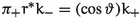 and
and  ;
; -
 and
and 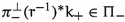 and moreover
 -
 is non-trivial.
 and
and  ;
; and
and  and moreover
 is non-trivial.
Lemma 6.2
Given blocks \((Z_\pm , \Sigma _\pm )\), a diffeomorphism  is a \(\vartheta \)-matching if and only if there exist hyper-Kähler triples \(\omega ^I_\pm , \omega ^J_\pm , \omega ^K_\pm \) on \(\Sigma _\pm \) such that \([\omega ^I_\pm ]\) is the restriction of a Kähler class from \(Z_\pm \), and
  is a \(\vartheta \)-hyper-Kähler rotation with respect to the triples.
Proof
If  is a \(\vartheta \)-hyper-Kähler rotation then taking
  satisfies the first two conditions in Definition 6.1, while
  .
.
For the converse, note that  is a nonzero element of \(\Pi _+\), but is not in
  . Therefore \(\Sigma _+\) has a holomorphic 2-form \(\omega ^J_+ + i\omega ^K_+\) with
  and
and  . By the Calabi–Yau theorem, there is a Ricci-flat Kähler metric
  .
.
Choosing \(\omega ^I_-, \omega ^J_-, \omega ^K_-\) analogously and normalising ensures that  ,
,  and
and  . Uniqueness of Ricci-flat Kähler metrics in their Kähler class implies (1.7), so
  is a hyper-Kähler rotation. \(\square \)
Note that in combination with Theorem 1.1, whenever we find a \(\vartheta \)-matching of a pair of building blocks we can also construct a pair of ACyl Calabi–Yau manifolds with a hyper-Kähler rotation. If we have also chosen a torus matching with gluing angle \(\vartheta \), and the blocks have any necessary involutions, then we have all the ingredients needed to apply Construction 1.10.
7.2 Marked K3s and configurations
To understand the topology of the extra-twisted connected sum M arising from some \(\vartheta \)-matching  of a pair of building blocks \(Z_+, Z_-\), we need to know not just some data about \(Z_\pm \) (described in Sect. 2.5), but also something about the action of
  ; for a start,
  clearly plays a role in the Mayer–Vietoris calculation of the cohomology of M (see Sect. 7.1).
At this point is convenient to switch to the language of marked K3 surfaces, i.e. choose isomorphisms \(h_\pm : L \rightarrow H^2(\Sigma _\pm )\) where L is a fixed copy of the unimodular lattice of signature (3, 19). Choices of markings of anticanonical divisors in building blocks in particular identify the polarising lattices \(N_\pm \) with primitive sublattices of L. Now, if we are given a \(\vartheta \)-hyper-Kähler rotation or \(\vartheta \)-matching  , then we could choose
  . Thus, we obtain a pair of embeddings of \(N_+\) and \(N_-\) into L, depending only on the choice of \(h_+\).
Definition 6.3
A configuration of polarising lattices \(N_+\), \(N_-\) is a pair of primitive embeddings \(N_\pm \hookrightarrow L\). Two configurations are equivalent if they are related by the action of the isometry group O(L).
So in these terms any hyper-Kähler rotation or matching has an associated configuration whose equivalence class is well-defined. As we see in Sect. 7, the configuration captures enough information that we can compute many topological invariants.
On the other hand, for a fixed pair of building blocks there is usually little chance of finding a matching. Following the pattern of [2, Section 6] and [12, Section 5], it is more fruitful to set up the matching problem as
Given \(\vartheta \in {\mathbb {R}}/2\pi {\mathbb {Z}}\) and a pair \({\mathcal {Z}}_+\), \({\mathcal {Z}}_-\) of sets of building blocks with fixed topological type and polarising lattices \(N_\pm \), which configurations of embeddings \(N_\pm \subset L\) arise from some matching of elements of \({\mathcal {Z}}_+\) and \({\mathcal {Z}}_-\)?
Using the Torelli theorem, we can reduce the problem of finding building blocks with a \(\vartheta \)-matching compatible with a given configuration to finding certain triples of classes in \(L_{\mathbb {R}}\).
Lemma 6.4
Let \((Z_\pm , \Sigma _\pm )\) be a pair of blocks, and let \(h_\pm : L \rightarrow H^2(\Sigma _\pm )\) be markings. Then, there exists a \(\vartheta \)-matching  with
with  if and only if there exists a triple of unit positive classes
  in \(L_{\mathbb {R}}\) such that
-

-
 , and
, and -
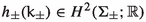 is the restriction of a Kähler class from \(Z_\pm \),
 -
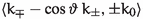 is the period of the marked K3 \((\Sigma _\pm , h_\pm )\).

 , and
, and is the restriction of a Kähler class from
  is the period of the marked K3
 Proof
Let  , which is a unit class perpendicular to
  and
and  . Let \(\omega ^J_- + i \omega ^K_-\) be the holomorphic 2-form on \(\Sigma _-\) in the cohomology class
  , and let \(\omega ^I_-\) be the unique Ricci-flat Kähler metric in
  . Then, \(\omega ^I_-, \omega ^J_-, \omega ^K_-\) is a hyper-Kähler triple. The closed complex 2-form \(\Omega ':= -(\cos \vartheta )\omega ^I_- + (\sin \vartheta )\omega ^J_- - i \omega ^K_-\) defines an integrable complex structure on \(\Sigma _-\). Let \(\Sigma '_-\) denote \(\Sigma _-\) equipped with this complex structure for which \(\Omega '\) is holomorphic. Then, \(\omega ':= -(\sin \vartheta )\omega ^I_- - (\cos \vartheta )\omega ^J_-\) is a Kähler form on \(\Sigma '_-\).
Now \(h_+ \circ h_-^{-1}: H^2(\Sigma '_-;{\mathbb {Z}}) \rightarrow H^2(\Sigma _+;{\mathbb {Z}})\) is an isometry that maps \([\Omega ']\) to  , and \([\omega ']\) to
  . Thus, \(h_+ \circ h_-^{-1}\) is a Hodge isometry, and by the Torelli theorem it is realised as
  for some biholomorphism
  . \(\square \)
Remark 6.5
Given a configuration of \(N_+\) and \(N_-\), we obtain lattice
containing \(N_+\) and \(N_-\) as primitive sublattices. In general, it is possible for W to fail to be primitive in L (see [2, Example No 8] for such a twisted connected sum), but for simplicity we will not look for such configurations in this paper. By only using examples of small rank and with W primitively embedded in L, the equivalence classes of the configurations are completely characterised just by the embeddings of \(N_\pm \) into W. This is a consequence of the following result of Nikulin [32, Theorem 1.12.4].
Theorem 6.6
Let W be an even non-degenerate lattice of signature \((t_+, t_-)\), and L an even unimodular lattice of indefinite signature \((\ell _+,\ell _-)\). If \(t_+ \le \ell _+\), \(t_- \le \ell _-\) and \(2{{\,\textrm{rk}\,}}W \le {{\,\textrm{rk}\,}}L\), then there exists a primitive embedding \(W \hookrightarrow L\), unique up to O(L).
7.3 Necessary conditions for matching
Let us next consider what necessary conditions Lemma 6.4 imposes on a configuration for it to be realised by a matching of blocks. Note first of all that one must have  , while the period
  is orthogonal to \(N_\pm \). Hence, \(\pi _\pm k_{\mp }\) is precisely \(\cos \vartheta \, k_\pm \), where \(\pi _\pm : L_{\mathbb {R}}\rightarrow N_\pm ({\mathbb {R}})\) is the orthogonal projection. Observe that \(\pi _+\pi _-: N_+({\mathbb {R}}) \rightarrow N_+({\mathbb {R}})\) is self-adjoint (since \(\langle x, \, \pi _+\pi _- y\rangle = \langle \pi _-x, \, \pi _- y \rangle \) is symmetric in \(x,y \in N_+\)) so \(N_+({\mathbb {R}})\) splits as a direct sum of eigenspaces.
Notation 6.7
For \(\psi \in {\mathbb {R}}\), let \(N_\pm ^\psi \subset N_\pm ({\mathbb {R}})\) denote the \((\cos \psi )^2\)-eigenspace of \(\pi _{\mp }\circ \pi _{\mp }\).
Clearly \(\pi _+\) maps \(N_+({\mathbb {R}})^\psi \) to \(N_-({\mathbb {R}})^\psi \), and is invertible if \(\psi \not = 0\). Of course, \(N_+({\mathbb {R}})^0 = N_-({\mathbb {R}})^0 = N_+({\mathbb {R}}) \cap N_-({\mathbb {R}})\). For any \(x \in N_+({\mathbb {R}})^\psi \) and \(y:= \pi _+x\)
In particular, it is necessary that  .
.
Here is a qualitative difference between the matching problem for rectangular twisted connected sums (\(\vartheta = \frac{\pi }{2}\)) and extra-twisted connected sums (\(\vartheta \not = \frac{\pi }{2}\)): in the former case we can choose  independently of each other, while in the latter case
  and
and  determine each other.
Remark
If the ambient space L were positive-definite, then the eigenvalues \(\lambda \) of \(\pi _+\circ \pi _-\) would obviously be forced to lie in [0, 1]. In a space of indefinite signature it could in general happen that
-
\(\lambda < 0\), if \(x \in N_+\) such that \(x^2\) and \((\pi _- x)^2\) have opposite sign, e.g. if \(N_\pm \) in hyperbolic space with bilinear form \(\left( {\begin{matrix} 0 &{} 1 \\ 1 &{} 0 \end{matrix}} \right) \) are spanned by \(x_+ = (2,1)\) and \(x_- = (1, -2)\), then \(\pi _{\mp } x_\pm = \pm \frac{3}{4}x_{\mp }\), and the unique eigenvalue of \(\pi _+\pi _-\) is \(-\frac{9}{16}\); or that
-
\(\lambda > 1\), if \(x \in N_+\) and \(\pi _- x \in N_-\) span an indefinite 2-dimensional subspace but \(x^2\) and \((\pi _- x)^2\) have the same sign, e.g. if we take \(N_\pm \) in the hyperbolic space to be the subspaces spanned by \(x_+ = (2,1)\) and \(x_- = (1,2)\), then \(\pi _{\mp } x_\pm = \frac{5}{4}x_{\mp }\), and the unique eigenvalue of \(\pi _+\pi _-\) is \(\frac{25}{16}\).
However, for matchings with the given configuration to exist, we saw above that there must exist some positive classes  , which are also orthogonal to the positive class
  . That forces \(N_+ + N_-\) to split as an orthogonal direct sum of its intersection with the orthogonal complement in L to the span of
  and
and  , which is negative definite, and the 2-dimensional positive definite span of
  and
and  . That forces all eigenvalues of \(\pi _+\pi _-\) to lie in [0, 1], so that they can be written as \((\cos \psi )^2\).
The existence of a \(\vartheta \)-matching with a given configuration may also impose constraints on the Picard lattices of the K3s \(\Sigma _\pm \), beyond the a priori condition that \({{\,\textrm{Pic}\,}}\Sigma _\pm \) contains \(N_\pm \). Let \(N_\pm ^{\not =\vartheta } \subset N_\pm \) denote the orthogonal complement of \(N_\pm ^\vartheta \). Then  because \(N_\pm ^{\not =\vartheta } \subset N_\pm \), while
  because
  . Therefore
is perpendicular to the period  of \(\Sigma _\pm \), i.e. \(\Lambda _\pm \subset {{\,\textrm{Pic}\,}}\Sigma _\pm \).
In summary, given a pair of families of building blocks \({\mathcal {Z}}_\pm \), to find some pair of elements \((Z_\pm , \Sigma _\pm ) \in {\mathcal {Z}}_\pm \) with a \(\vartheta \)-matching  it is necessary that we can take the marked \((Z_\pm , \Sigma _\pm , h_\pm )\) such that
-
(i)
The intersection of \(N_\pm ({\mathbb {R}})^\vartheta \) with the image \({\mathcal {K}}_{Z_\pm } \subset L_{\mathbb {R}}\) of the Kähler cone of \(Z_\pm \) is non-empty. Moreover, if \(\vartheta \not = \frac{\pi }{2}\) then the intersection of \(\epsilon \pi _- (N_+ \cap {\mathcal {K}}_{Z_+})\) and \({\mathcal {K}}_{Z_-}\) is non-empty too, where
$$\begin{aligned} \epsilon {:}{=} (\text {sign of } \cos \vartheta ) \in \{\pm 1\}. \end{aligned}$$ -
(ii)
\(\Sigma _\pm \) is \(\Lambda _\pm \)-polarised.
7.4 Sufficient conditions for existence of matching
On the other hand, for the family \({\mathcal {Z}}_\pm \) to be \((\Lambda _\pm , {{\,\textrm{Amp}\,}}_{{\mathcal {Z}}_\pm })\)-generic for some open cone \({{\,\textrm{Amp}\,}}_{{\mathcal {Z}}_\pm } \subset N_\pm ({\mathbb {R}})\) (Definition 2.27) says roughly that a generic \(\Lambda _\pm \)-polarised K3 can be embedded as an anticanonical divisor in some block \(Z_\pm \in {\mathcal {Z}}_\pm \), and moreover in such a way that the Kähler cone of \(Z_\pm \) contains \({{\,\textrm{Amp}\,}}_{{\mathcal {Z}}_\pm }\). This genericity property is enough to obtain a sufficient condition for the existence of \(\vartheta \)-matchings.
Theorem 6.10
Let \({\mathcal {Z}}_\pm \) be a pair of families of building blocks with polarising lattices \(N_\pm \), and \(\vartheta \in {\mathbb {R}}{\setminus } \frac{\pi }{2}{\mathbb {Z}}\). Let \(N_\pm \hookrightarrow L\) be a configuration of the polarising lattices, and define \(\Lambda _\pm \) as in (6.9). Suppose that the family \({\mathcal {Z}}_\pm \) is \((\Lambda _\pm , {{\,\textrm{Amp}\,}}_{{\mathcal {Z}}_\pm })\)-generic. If
then there exist \((Z_\pm , \Sigma _\pm ) \in {\mathcal {Z}}_\pm \) with an angle \(\vartheta \) K3 matching  with the prescribed configuration.
Proof
The proof uses the same basic idea as in the proof of the \(\vartheta = \frac{\pi }{2}\) case from [2, Proposition 6.18], but the way that  and
and  determine each other in this case makes it slightly different.
Let \(W_\pm \) be the orthogonal complement of \(N_\pm ({\mathbb {R}})^\vartheta \) in \(N_+({\mathbb {R}})^\vartheta \oplus N_-({\mathbb {R}})^\vartheta \), and T the orthogonal complement of \(N_+({\mathbb {R}}) + N_-({\mathbb {R}})\) in \(L_{\mathbb {R}}\). \(W_\pm \) and T all have signature \((1,{{\,\textrm{rk}\,}}-1)\). Note that \(W_\pm \oplus T\) is the orthogonal complement of \(\Lambda _\pm \). Thus, a pair of real lines in the positive cones of \(W_\pm \) and T span a positive-definite 2-plane in \(\Lambda _\pm ^\perp \), so
can be regarded as a submanifold of \(G_{\Lambda _\pm }\). Analogously to [2, Proposition 6.18] it is an analytic, totally real submanifold. Moreover, because \(\Lambda _\pm ^\perp \) is exactly \(W_\pm \oplus T\),
Therefore the intersection of the submanifold \({\mathbb {P}}\bigl (W_\pm ^+\bigr )\times {\mathbb {P}}\bigl (T^+\bigr ) \subset G_{\Lambda _\pm }\) with the subset \(U_{{\mathcal {Z}}_\pm } \subset G_{\Lambda _\pm }\) from Definition 2.27 is an open dense subset of \({\mathbb {P}}\bigl (W_\pm ^+\bigr )\times {\mathbb {P}}\bigl (T^+\bigr )\).
Now we wish to find \((\ell _+, \ell _0) \in {\mathbb {P}}(N_+({\mathbb {R}})^\vartheta ) \times {\mathbb {P}}(T^+)\) such that
-
(i)
\(\ell _+ \in {{\,\textrm{Amp}\,}}_{{\mathcal {Z}}_+}\),
-
(ii)
\(\epsilon \pi _- \ell _+ \in {{\,\textrm{Amp}\,}}_{{\mathcal {Z}}_-}\),
-
(iii)
\(\big (w_+(\ell _+), \ell _0 \big ) \in \left( {\mathbb {P}}\bigl (W_+^+\bigr )\times {\mathbb {P}}\bigl (T^+\bigr )\right) \cap U_{{\mathcal {Z}}_+}\),
-
(iv)
\(\big (w_-(\ell _+), \ell _0 \big ) \in \left( {\mathbb {P}}\bigl (W_-^+\bigr )\times {\mathbb {P}}\bigl (T^+\bigr )\right) \cap U_{{\mathcal {Z}}_-}\),
where \(w_\pm : N_+({\mathbb {R}})^\vartheta \rightarrow W_\pm \) are the orthogonal projections (which are both isomorphisms since \(\vartheta \not = \frac{\pi }{2}\)). The first two conditions define open subsets whose intersection is non-empty by the hypothesis (6.11). The intersection with the open dense subsets defined by the last two conditions is therefore non-empty. Hence, there is a pair \((\ell _+, \ell _0)\) satisfying (i)–(iv).
By the definition of \({\mathcal {Z}}_\pm \) being \((\Lambda _\pm , {{\,\textrm{Amp}\,}}_{{\mathcal {Z}}_\pm })\)-generic, this means there exist \((Z_\pm , \Sigma _\pm ) \in {\mathcal {Z}}_\pm \) with periods \(\big (w_+(\ell _\pm ), \ell _0 \big )\) such that \({{\,\textrm{Amp}\,}}_{{\mathcal {Z}}_\pm }\) is contained in the image of Kähler cone of \(Z_\pm \) Taking  ,
,  and
and  to be the unit norm representatives of \(\ell _+\), \(\epsilon \pi _-\ell _+\) and \(\ell _0\), respectively, we can therefore apply Lemma 6.4 to obtain the desired \(\vartheta \)-matching
  . \(\square \)
7.5 Configuration angles and pure configurations
The following invariants of a configuration turn out to have several uses.
Definition 6.12
Given a configuration \(N_+, N_- \subset L\), let \(A_\pm : L_{\mathbb {R}}\rightarrow L_{\mathbb {R}}\) denote the reflection of \(L_{\mathbb {R}}:= L \otimes {\mathbb {R}}\) in \(N_\pm \) (with respect to the intersection form of \(L_{\mathbb {R}}\); this is well-defined since \(N_\pm \) is non-degenerate). Suppose that \(A_+ \circ A_-\) preserves some decomposition \(L_{\mathbb {R}}= L^+ \oplus L^-\) as a sum of positive- and negative-definite subspaces. Then the configuration angles are the arguments \(\alpha ^+_1, \alpha ^+_2, \alpha ^+_3\) and \(\alpha ^-_1, \ldots , \alpha ^-_{19}\) of the eigenvalues of the restrictions \(A_+ \circ A_-: L^+ \rightarrow L^+\) and \(A_+ \circ A_-: L^- \rightarrow L^-\), respectively.
Note that if the configuration is to be realised by a \(\vartheta \)-hyper-Kähler rotation, then \(A_+ \circ A_-\) preserves the decomposition of \(L_{\mathbb {R}}\) into the subspaces that self-dual and anti-self-dual with respect to the hyper-Kähler metric, so the configuration angles are defined. Further, the necessary condition (i) from Sect. 6.3 can be expressed in terms of the configuration angles as requiring that \(\alpha ^+_1, \alpha ^+_2, \alpha ^+_3\) are precisely 0 and \(\pm 2\vartheta \).
In view of Proposition 3.7, the hypothesis that the family \({\mathcal {Y}}_\pm \) is \((\Lambda _\pm , {{\,\textrm{Amp}\,}}_{{\mathcal {Y}}_\pm })\)-generic (for some cone \({{\,\textrm{Amp}\,}}_{{\mathcal {Y}}_\pm }\)) is easiest to verify in the case of configurations where \(\Lambda _\pm = N_\pm \). This amounts to requiring that \(N_{\mp }^{\not =\vartheta }\) is contained in \(N_\pm \), or equivalently that \(N_{\mp }\) is spanned (at least rationally) by \(N_{\mp }^0 = N_+ \cap N_-\) and \(N_{\mp }^\vartheta \). Noting that for \(0< \vert \psi \vert < \frac{\pi }{2}\)
this is in turn equivalent to requiring that the only nonzero configuration angles are \(\pm 2\vartheta \). This is in particular the case if \(N_\pm ^\vartheta = N_\pm \); we refer to such configurations as having “pure angle \(\vartheta \)”.
Configurations with pure angle \(\frac{\pi }{2}\) are very easy to produce (as long as \({{\,\textrm{rk}\,}}N_+ + {{\,\textrm{rk}\,}}N_- \le 11\)): simply apply Theorem 6.6 to embed the perpendicular direct sum \(N_+ \perp N_-\) primitively in L. On the other hand, for \(\vartheta \not = \frac{\pi }{2}\), the existence of a pure angle \(\vartheta \) configuration of a given pair of lattices \(N_+\), \(N_-\) is a non-trivial condition. To be able to define a bilinear form on \(W:= N_+ \oplus N_-\) that restricts to the prescribed one on \(N_\pm \) and such that \(N_\pm ^\vartheta = N_\pm \), it is necessary but not sufficient that the ranks be equal.
Consider the case when \({{\,\textrm{rk}\,}}N_\pm \) both have rank 1, with generator \(n_\pm \) (chosen to be positive, i.e. \(n_\pm \in {{\,\textrm{Amp}\,}}_{{\mathcal {Z}}_\pm }\)). Then there is only a single cross-term to choose in W, and by (6.8) we must set
Thus, in this case W exists if and only if the RHS is an integer.
Example 6.15
We can make a \(\vartheta = \frac{\pi }{4}\) or \(\vartheta = \frac{3\pi }{4}\) matching of the involution block from Example 3.25\(_1\) and a regular block from Example 3.8\(^4_1\) using
(This leads to a 2-connected \(\tfrac{\pi }{4}\)-twisted connected sum with \(b_3(M) = 134\) and p(M) divisible by 24, see Table 4).
Remark 6.17
If there does exist a pure angle \(\vartheta \) configuration between the polarising lattices, then for \(\vartheta \not = \frac{\pi }{2}\) it does not need to be unique, and different pure angle matchings of blocks from the same families can lead to non-diffeomorphic \(\vartheta \)-twisted connected sums; see Examples 8.17 and 8.18.
Let us think a moment about the meaning of changing the sign of \(\vartheta \) or replacing it by a complementary angle. For a start, the condition in Definition 6.1 for  to be a \(\vartheta \)-matching is actually independent of the sign of \(\vartheta \), which is related to the earlier observation that a \(\pm \vartheta \)-twisted connected sums of phase rotated ACyl Calabi–Yaus are (orientation-reversing) diffeomorphic. So the sign is unimportant.
There are several natural ways to modify a matching in order to complement the angle. We could change the signs of the cross-terms in W like in (6.16) while keeping everything else the same, or equivalently, we could change the sign of the marking on \((\Sigma _+, I_+)\) (keeping W the same, but multiplying \({{\,\textrm{Amp}\,}}_{{\mathcal {Z}}_\pm }\) by \(-1\)). Alternatively, we could replace the block \(Z_+\) by its complex conjugate; if we keep the marking the same, then \({{\,\textrm{Amp}\,}}_{Z_+}\) is multiplied by \(-1\). This is precisely the same way of relating extra-twisted connected sums with complementary angles as in Remark 1.12. Any of these changes leaves the cohomology and \(p_1\) of the resulting \(G_2\)-manifolds unchanged, so we will not be concerned with distinguishing between complementary angles in the examples.
8 Topology
We now turn to the problem of computing topological properties of extra-twisted connected sums. All our computations will be expressed in terms of data of the building blocks listed in Tables 1, 2 and 3 (see Sect. 2.5), along with the choice of torus isometry, and the configuration of the hyper-Kähler rotation in the sense of Definition 6.3.
The invariants we compute are the integral cohomology, torsion linking form, and a spin characteristic class (more or less equivalent to the first Pontryagin class). Computing the cohomology is routine, though the details of understanding in particular the torsion in \(H^4\) are a bit tedious. The computation of the spin characteristic class is more involved, and takes up Sects. 7.2–7.5. The pay-off is that—as explained in Sect. 7.8—the invariants we compute are sufficient to apply classification results for 2-connected 7-manifolds to completely determine the diffeomorphism types of most examples considered in this paper.
8.1 Mayer–Vietoris generalities
It seems inevitable that computing the full integral cohomology of an extra-twisted connected sum will involve some case by case checking for different gluing angles \(\vartheta \). However, some parts of the computation are common to all non-rectangular extra-twisted connected sums.
Let us briefly recap the context. We are gluing two ACyl \(G_{2}\)-manifolds \(M_+\) and \(M_-\), each of which is either a product \(S^1_{\xi _\pm } \times V_\pm \) or a mapping torus \(S^1_\xi \mathbin {\widetilde{\times }} V_\pm = (S^1_{\xi _\pm } \times V_\pm )/(a \times \tau _\pm )\) of an involution \(\tau _\pm \) (a denotes the antipodal map on the circle). The asymptotic cross-section is of the form \(S^1_{\xi _\pm } \times S^1_{\zeta _\pm } \times \Sigma \) or \((S^1_{\xi _\pm } \times S^1_{\zeta _\pm })/(a \times a)\) accordingly. To make the construction, we use a torus matching  and hyper-Kähler rotation
  to identify the asymptotic cross-section from each side with a single \(T^2 \times \Sigma \). We now want to apply the Mayer–Vietoris theorem to \(M = M_+ \cup M_-\), with \(M_+ \cap M_- \simeq T^2 \times \Sigma \).
We set up notation for various cohomology classes on this cross-section \(T^2 \times \Sigma \), mirroring that used in Sect. 2. On the asymptotic cross-section \(S^1_{\xi _\pm } \times S^1_{\zeta _\pm } \times \Sigma \) of \(S^1_{\xi _\pm } \times V_\pm \) let \({\textbf{v}}_\pm \in H^1(S^1_{\xi _\pm } \times S^1_{\zeta _\pm } \times \Sigma )\) correspond to the generator of the “external” factor \(H^1(S^1_{\xi _\pm })\), and let \({\textbf{u}}_\pm \in H^1(S^1_{\xi _\pm } \times S^1_{\zeta _\pm } \times \Sigma )\) correspond to the generator of the “internal” factor \(H^1(S^1_{\zeta _\pm })\). If \(V_\pm \) has an involution, then like in Notation 2.19 we abuse notation to denote cohomology classes on the asymptotic cross-section \((S^1_{\xi _\pm } \times S^1_{\zeta _\pm })/(a \times a)\) of \(S^1_\xi \mathbin {\widetilde{\times }} V_\pm \) identically with their pull-backs to \(S^1_{\xi _\pm } \times S^1_{\zeta _\pm } \times \Sigma \). Thus, \(2{\textbf{v}}_\pm \) and \(2{\textbf{u}}_\pm \) denote primitive elements in \(H^1(T^2 \times \Sigma )\) in this case, but the subgroup they generate has index 2. In particular, \({\textbf{v}}_-, {\textbf{u}}_- \in H^1(T^2 \times \Sigma )\) make sense only when \(M_-\) is not a mapping torus, like for \(\tfrac{\pi }{4}\)-matchings in Sect. 7.6 (“square” ones with \(b_+ = 1\) and \(b_- = 0\) in terms of the discussion in Sect. 1.3).
\(H^1(M_\pm ) \rightarrow H^1(T^2 \times \Sigma )\) is an isomorphism onto the cyclic subgroup of \(H^1(T^2)\) dual to the internal circle factor, i.e. the image is generated by \({\textbf{v}}_\pm \) or \(2{\textbf{v}}_\pm \) depending on whether \(M_\pm \) comes from an ordinary block or an involution block. The images never intersect, so \(H^1(M) = 0\). The sum of the images is primitive precisely for the arrangements when M is simply connected; otherwise the contribution to \(H^2(M)\) is (obviously) the finite cyclic group \(\pi _1(M)\), but we ignore this case from now on.
\(H^2(M_\pm ) \rightarrow H^2(T^2 \times \Sigma )\) is an isomorphism onto \(N_\pm \subset H^2(\Sigma )\), regardless of whether \(M_\pm \) comes from an ordinary or an involution block. Thus, \(H^2(M) = N_+ \cap N_-\), and we get a contribution \({\mathbb {Z}}\oplus L/(N_+ + N_-)\) to \(H^3(M)\). Whether this is torsion-free depends on the choice of push-out W in the matching, and on whether we embed W primitively in L or not.
Since \(H^3(M_\pm )\) are torsion-free, there is no other contribution to the torsion in \(H^3(M)\). Thus, we get M 2-connected if and only if we use building blocks with \(K_\pm = 0\) and a configuration such that \(N_+ \cap N_- = 0\) and \(N_+ \oplus N_-\) is primitive in L.
To determine \(H^3(M)\) we only need to deal with \(H^3(M_\pm ) \rightarrow H^3(T^2 \times \Sigma )\) rationally; the contribution to the torsion in \(H^4(M)\) will have to be dealt with case by case. The image of \(H^3(M_\pm ; {\mathbb {Q}})\) is the Lagrangian \({\textbf{v}}_\pm N_\pm \oplus {\textbf{u}}_\pm T_\pm \subset H^3(T^2 \times \Sigma ; \, {\mathbb {Q}})\). Since
for \({\textbf{v}}_+ n_+ + {\textbf{u}}_+ t_+\) to equal \({\textbf{v}}_- n_- + {\textbf{u}}_- t_-\) for some \(n_\pm \in N_\pm \) and \(t_\pm \in T_\pm \) implies that \(\pi _\pm n_{\mp } = \cos \vartheta n_\pm \), and thus, \(n_\pm \in N_\pm ^\vartheta \) in Notation 6.7. Hence, the dimension of the intersection of the images of \(H^3(M_\pm , {\mathbb {Q}})\) equals \(d_\vartheta = {{\,\textrm{rk}\,}}N_+^\vartheta = {{\,\textrm{rk}\,}}N_-^\vartheta \) (or the multiplicity of \(\vartheta \) as a configuration angle (6.13)). On the other hand, the kernel in \(H^3(M; {\mathbb {Q}})\) is the \(\tau \)-invariant subgroup \(H^3(Z;{\mathbb {Q}})^\tau \), or just \(H^3(Z;{\mathbb {Q}})\) in the case of an ordinary block. Denoting the dimension of that by \(b_3^+(Z_\pm )\), we obtain
Remark 7.3
\(b_3^+(Z_\pm )\) is always even since \(H^3(Z_\pm )^\tau \subseteq H^3(Z_\pm )\) is symplectic. Therefore
Further, \(\rho _+ + \rho _- = {{\,\textrm{rk}\,}}N_+^\frac{\pi }{2} + {{\,\textrm{rk}\,}}N_-^\frac{\pi }{2} \!\!\mod 2\), the rank of the perpendicular parts. Hence, the “semi-characteristic” of M equals \(d_\vartheta + {{\,\textrm{rk}\,}}N_+^\frac{\pi }{2} + {{\,\textrm{rk}\,}}N_-^\frac{\pi }{2}\).
Remark 7.4
For \(\vartheta = \frac{\pi }{2}\) we should interpret \(d_\vartheta \) to mean \({{\,\textrm{rk}\,}}N_+^\frac{\pi }{2} + {{\,\textrm{rk}\,}}N_-^\frac{\pi }{2} = {{\,\textrm{rk}\,}}(N_+ \cap T_-) + {{\,\textrm{rk}\,}}(N_- \cap T_+)\). In the case of an orthogonal matching we get \(d_\vartheta = \rho _+ + \rho _- - 2b_2(M)\), and (7.2) recovers the claim from [1, (8.56)] that \(b_2(M) + b_3(M) = 23 + b_3(Z_+) + b_3(Z_-)\) in this setting. (And from Remark 7.3 we get that the semi-characteristic is even for any rectangular twisted connected sum, equivalent to claim (i) of the introduction.)
Remark 7.5
When the involution blocks are pleasant, then \(H^4(M_\pm )\) is torsion-free, so the image \(\delta (H^3(T^2 \times \Sigma ))\) of the Mayer–Vietoris boundary map is a direct summand of \(H^4(M)\), and contains all torsion in \(H^4(M)\).
In Sects. 7.6–7.7 we study \(\delta (H^3(T^2 \times \Sigma ))\) in further detail in the cases \(\vartheta = \frac{\pi }{4}\) and \(\frac{\pi }{6}\). We can make a general statement about the torsion linking form \(b_M\) (cf. [33, Propositon 3.2]).
Lemma 7.6
Let \(M^7 = M_+ \cup _X M_-\) be a gluing of manifolds with boundary X, and let \(I_\pm \subseteq H^3(X)\) be the image of \(H^3(M_\pm )\). Let \(p_1, p_2 \in H^3(X)\) be classes that are torsion modulo \(I_+ + I_-\), so that their images \(\delta (p_1), \delta (p_2) \in H^4(M)\) under the Mayer–Vietoris boundary map are torsion classes. Then we can write \(mp_1 = p_1^+ - p_1^-\) for some \(m \in {\mathbb {Z}}\) and \(p_1^\pm \in I_\pm \), and
Proof
To compute the torsion linking form, we first need a pre-image of \(\delta (p_1)\) under the Bockstein map \(\beta : H^3(M; {\mathbb {Q}}/{\mathbb {Z}}) \rightarrow H^4(M; {\mathbb {Z}})\). First let \(q^\pm \in H^3(M_\pm ; {\mathbb {Q}})\) be a pre-image of \(\frac{1}{m}p_1^\pm \in H^3(X; {\mathbb {Q}})\).
The Mayer–Vietoris sequences with coefficients \({\mathbb {Z}}, {\mathbb {Q}}\) or \({\mathbb {Q}}/{\mathbb {Z}}\) form a commuting periodic grid with the change-of-coefficients sequences. It is a general feature of such grids that equality of the images in \(H^3(X; {\mathbb {Q}})\) of \(p_1 \in H^3(X; {\mathbb {Z}})\) and \((q^+, q^-) \in H^3(M_+; {\mathbb {Q}}) \oplus H^3(M_-; {\mathbb {Q}})\) implies that there exists \(q \in H^3(M; {\mathbb {Q}}/{\mathbb {Z}})\) such that \(q_{\vert M_\pm } = \frac{1}{m}q^\pm \in H^3(M_\pm ; {\mathbb {Q}}/{\mathbb {Z}})\) while \(\beta (q) = -\delta (p_1)\).
More explicitly, pick cochain representatives \(\sigma \) of \(p_1\) and \(\rho ^\pm \) of \(q^\pm \). We can write \(\sigma = \tau ^+_{X} - \tau ^-_{\vert X}\) for some \((\tau ^+, \tau ^-) \in C^3(M_+; {\mathbb {Z}}) \oplus C^3(M_-;{\mathbb {Z}})\). Meanwhile the cochain \(m\sigma - \rho ^+_{\vert X} + \rho ^-_{\vert X}\) on X is exact, so we can pick a pre-differential \(\nu \in C^2(X; {\mathbb {Z}})\), which we in turn write as \(\nu = \mu ^+_{\vert X} - \mu ^-_{\vert X}\) for some \((\mu ^+, \mu ^-) \in C^2(M_+; {\mathbb {Z}}) \oplus C^2(M_-; {\mathbb {Q}}/{\mathbb {Z}})\). Then \(\left( \frac{1}{m}(\rho ^++ d\mu ^+)-\tau ^+, \frac{1}{m}(\rho ^- +d\nu ^-)-\tau ^- \right) \) has a pre-image in \(C^3(M; {\mathbb {Q}})\). That is closed mod \({\mathbb {Z}}\), and we can take q to be the class represented by the mod \({\mathbb {Z}}\) reduction.
Using \(-q\) as a pre-image of \(\delta (p_1)\) in the definition of the torsion linking form now gives
\(\square \)
8.2 The spin characteristic class
Apart from the integral cohomology, the main invariant of an extra-twisted connected sum that we are interested in is the spin characteristic class \(p(M) \in H^4(M)\). It is a refinement of the first Pontryagin class \(p_1(M)\) in the sense that \(p_1(M) = 2p(M)\) (so in the absence of 2-torsion in \(H^4(M)\), p(M) is in fact determined by \(p_1(M)\)), see e.g. [11, Subsection 2.1]. Here are essentially the only facts we need about p(M) beyond it being a characteristic class.
Lemma 7.7
(See [11, Lemmas 2.2 and 2.39])
-
(i)
\(p(M) \in H^4(M)\) is even for any spin manifold of dimension \(\le 7\).
-
(ii)
\(p(M) = -c_2(M)\) for any SU-manifold.
While we should remember that the building blocks \(Z_\pm \) are not spin (because \(c_1(Z_\pm ) = PD(\Sigma )\) is primitive, and in particular odd), nevertheless \(c_2(Z_\pm ) \in H^4(Z_\pm )\) is always even, see [7, Lemma 5.10]. Our plan is to think of p(M) as the result of patching up the classes \(-c_2(Z_\pm ) \in 2H^4(Z_\pm )\), and we make this precise in Theorem 7.21. However, even once we have a formula for p(M), one needs to look carefully at the Mayer–Vietoris sequence to understand what it means (e.g. what the greatest divisor in \(H^4(M)\) is), which we do in Sects. 7.6–7.7.
To apply classification results for 2-connected manifolds (see Sect. 7.8), all we need to know about p(M) is the class of \((H^4(M), p(M))\) up to isomorphisms of abelian groups with a distinguished element. If \(H^4(M)\) is torsion-free this simply amounts to determining the greatest integer dividing p(M) (while in general one would also need to capture information such as the greatest integer dividing p(M) modulo torsion). Since the image of p(M) in \(H^4(\Sigma )\) is divisible by exactly \(\chi (K3) = 24\), we effectively care about the value of p(M) only modulo 24.
This proves practical to evaluate when \(c_2(Z_\pm )\) has been computed in the form (2.21), as we have done for all the pleasant involution blocks in Sects. 2 and 5. Recall also from Remarks 3.23 and 5.18 that the class \(\widehat{B}(h) \in H^3_{cpt}(V)\) from (2.24) vanishes in all those examples.
Theorem 7.8
Write \(c_2(Z_\pm ) = g_\pm {{\bar{c}}}_2(Z_\pm ) + 24h_\pm \) as in (2.21), and suppose that \(h_\pm \) is \(\tau \)-invariant with \(\widehat{B}_\pm (h_\pm ) = 0\). Then
where \(\delta : H^3(T^2 \times \Sigma ) \rightarrow H^4(M)\) is the Mayer–Vietoris snake map.
Note that \({{\bar{c}}}_2(Z_\pm ) \in N_\pm ^* = L/T_\pm \) is always even, say \({{\bar{c}}}_2(Z_\pm ) = 2y_\pm \mod T_\pm \) for some \(y_\pm \in L\). Because the image of \(H^3(M_\pm ) \rightarrow H^3(T^2 \times \Sigma )\) always contains \(2{\textbf{u}}_\pm T_\pm \) (regardless of whether \(M_\pm \) is of the form \(S^1 \times V_\pm \) or \(S^1_\xi \mathbin {\widetilde{\times }} V_\pm \)), the value of the Mayer–Vietoris map \(\delta : H^3(T^2 \times \Sigma ) \rightarrow H^4(M)\) on \(2{\textbf{u}}_\pm y_\pm \) is independent of the choice of \(y_\pm \), and can be interpreted as a well-defined element \(\delta ({\textbf{u}}_\pm {{\bar{c}}}_2(Z_\pm )) \in H^4(M)\). (But there is in general no guarantee that these are even elements of \(H^4(M)\), even though their sum must be even, see Remarks 7.20 and 7.33.)
We will prove Theorem 7.8 in the next three subsections. In practice we apply the following special case.
Corollary 7.9
If in addition the building blocks \(Z_+\) and \(Z_-\) are both pleasant then the equivalence class of \(p(M) \in H^4(M)\) (modulo isomorphisms of the abelian group \(H^4(M)\)) is determined by
where \(I_\pm \) are the images of \(H^3(M_\pm )\). In particular, the greatest integer dividing p(M) is \(\gcd (24, n)\), where n is the greatest integer dividing (7.10).
Proof
We noted in Remark 7.5 that if \(Z_+\) and \(Z_-\) are pleasant then the image of \(\delta \) is a direct summand in \(H^4(M)\). \(\square \)
If \(M_\pm = S^1 \times V\) (i.e. does not involve dividing by an involution) then \(I_\pm \) is simply \({\textbf{v}}_\pm N_\pm \oplus {\textbf{u}}_\pm T_\pm \), while if \(M_\pm = S^1_\xi \mathbin {\widetilde{\times }} V_\pm \) and comes from a pleasant involution block then \(I_\pm \) is determined in Lemma 2.20(ii). However, even in the auspicious setting of Corollary 7.9, we still need to work out more details about \(\delta (H^3(T^2 \times \Sigma )) \cong H^3(T^2 \times \Sigma )/(I_+ + I_-)\).
That will have to proceed case by case for different choices of gluing angle \(\vartheta \) and torus isometry (see in particular Propositions 7.29 and 7.37), but let us point out an important qualitative difference between the cases \(\vartheta = \frac{\pi }{2}\) and \(\vartheta \not = \frac{\pi }{2}\): For rectangular TCS, the images of \(\delta ({\textbf{u}}_+{{\bar{c}}}_2(Z_+))\) and \(\delta ({\textbf{u}}_-{{\bar{c}}}_2(Z_-))\) belong to two different direct summands in \(H^4(M)\) (the respective images of the push-forward maps \(H^4_{cpt}(M_\pm ) \rightarrow H^4(M)\)), so that it suffices to compute the greatest divisors separately and then take their greatest common divisor. But for extra-twisted connected sums the images of \(H^4_{cpt}(M_\pm ) \rightarrow H^4(M)\) can overlap, so there can be cancellation between \(\delta ({\textbf{u}}_+{{\bar{c}}}_2(Z_+))\) and \(\delta ({\textbf{u}}_-{{\bar{c}}}_2(Z_-))\), and we need to know both terms precisely.
8.3 Gluing vertical cohomology classes
Let
the subspace of classes whose images under \(\gamma _\pm : H^4(M_\pm ) \rightarrow H^4(T^2 \times \Sigma )\), the pull-back by the inclusion \(T^2 \times \Sigma \hookrightarrow M_\pm \), agree. At the most elementary level, the problem we need to deal with in describing p(M) is that the map \(H^4(M) \rightarrow H^4(M_+) \oplus H^4(M_-)\) in the Mayer–Vietoris sequence, whose image is \(H^4(M_+) \oplus _0 H^4(M_-)\), does not have a canonical right inverse \({H^4(M_+) \oplus _0 H^4(M_-)} \rightarrow H^4(M)\). Thus, it is not possible to determine p(M) just from its restrictions \(p(M_+)\) and \(p(M_-)\). We wish to exploit that we do not just know \(p(M_\pm ) \in H^4(M_\pm )\), we also know \(p(S^1_\xi \mathbin {\widetilde{\times }} Z) \in H^4(S^1_\xi \mathbin {\widetilde{\times }} Z)\) which contain much more information. To be able to reconstruct p(M) from that, we further need to exploit that \(p(S^1_\xi \mathbin {\widetilde{\times }} Z)\) is in some sense a “vertical” class.
Certainly, the restriction of p(M) to a neighbourhood of \(S^1 \times \Sigma \subset S^1_\xi \mathbin {\widetilde{\times }} Z\) is a pull-back of \(p(\Sigma ) \in H^4(\Sigma )\). Now given cocycles on \(S^1_\xi \mathbin {\widetilde{\times }} Z_+\) and \(S^1_\xi \mathbin {\widetilde{\times }} Z_-\) whose restrictions to neighbourhoods of \(S^1 \times \Sigma \) are pull-backs of the same cocycle on \(\Sigma \), we could patch their pull-backs to \(M_\pm \) to a cocycle on M. The computation in [2, Proposition 4.20] of p(M) of a rectangular TCS is carried out in terms of a gluing map [2, Definition 4.15] described in these terms, but it is complicated and does not adapt well to the XTCS setting. Instead we wish to define essentially the gluing map in terms of pull-backs of maps between certain auxiliary spaces.
To this end, we first consider a space \(S^1 {\widehat{\times }} Z\) obtained from \(S^1_\xi \mathbin {\widetilde{\times }} Z\) by collapsing the external circle factor over \(\Sigma \subset Z\), and the projection map \({\rho : S^1_\xi \mathbin {\widetilde{\times }} Z \rightarrow S^1 {\widehat{\times }} Z}\). (A cochain on \(S^1_\xi \mathbin {\widetilde{\times }} Z\) that near \(\Sigma \) is a pull-back of a cochain on \(\Sigma \) is thus roughly the same thing as a pull-back of a cochain from \(S^1 {\widehat{\times }} Z\).)
Further, given a pair of blocks that are used to form an extra-twisted connected sum M, let \(R:= S^1 {\widehat{\times }} Z_+ \cup _\Sigma S^1 {\widehat{\times }} Z_-\). We can define a collapsing map
as well as obvious inclusion maps
By Mayer–Vietoris,
is an isomorphism onto the subgroup \(H^4(S^1 {\widehat{\times }} Z_+) \oplus _0 H^4(S^1 {\widehat{\times }} Z_-)\) of pairs with equal image in \(H^4(\Sigma )\). Thus composing the inverse with \(\kappa *\) gives a canonical way to glue elements of \(H^4(S^1 {\widehat{\times }} Z_+) \oplus _0 H^4(S^1 {\widehat{\times }} Z_-)\).
In a sense, this repackages the problem of gluing classes in \(H^4(S^1_\xi \mathbin {\widetilde{\times }} Z_\pm )\) as a problem of finding pre-images of those classes in \(H^4(S^1 {\widehat{\times }} Z_\pm )\). The issue now is that while \(\rho ^*: H^4(S^1 {\widehat{\times }} Z_\pm ) \rightarrow H^4(S^1_\xi \mathbin {\widetilde{\times }} Z)\) is surjective, it is certainly not injective. We could now ask ourselves for which subsets of \(H^4(S^1_\xi \mathbin {\widetilde{\times }} Z)\) there is a canonical right inverse to \(\rho ^*\), and try to give an answer in terms of certain kinds of “vertical” classes (e.g. \(\rho _*\) is injective on the kernel of a natural map \(H^4(S^1 {\widehat{\times }} Z_\pm ) \rightarrow H^3_{cpt}(V_\pm )\)).
Something that is good enough for our purposes is to define a map
as follows. If x is a \(\tau \)-invariant class, pick a cochain representative \(\alpha \) whose restriction to a neighbourhood of \(\Sigma \) is a pull-back of a cochain on \(\Sigma \). Then the cocycle \(\alpha + \tau ^* \alpha \) on \(S^1 \times Z\) descends to \(S^1_\xi \mathbin {\widetilde{\times }} Z\). Because its restriction to a neighbourhood of the collapsing set \(S^1 \times \Sigma \) is a pull-back from \(\Sigma \), it is moreover a pull-back of a cocycle on \(S^1 {\widehat{\times }} Z\). The resulting class \(\widehat{2x} \in H^4(S^1 {\widehat{\times }} Z)\) is clearly independent of the choice of representative \(\alpha \) of x. Because \(H^4(Z)\) is assumed to be torsion-free, it then depends only on 2x (and not on x).
Definition 7.12
Define
to be the composition of \(2x \mapsto \widehat{2x}\), the inverse of \((j_+^*, j_-^*)\), and the pull-back \(\kappa ^*: H^4(R) \rightarrow H^4(M)\).
In Theorem 7.21, we express p(M) as a gluing of \(c_2(Z_\pm )\) in this sense, but to prove it we need to know something about how \(\widehat{c_2(Z_\pm )} \in H^4(S^1 {\widehat{\times }} Z_\pm )\) relate to some actual bundles.
8.4 Pre-image of the vertical tangent bundle
It is natural to ask whether the pull-back of \(\widehat{c_2(Z_\pm )}\) in \(H^4(S^1_\xi \mathbin {\widetilde{\times }} Z_\pm )\) equals the second Chern class of the vertical tangent bundle \(T_{vt}(S^1_\xi \mathbin {\widetilde{\times }} Z_\pm )\). We will in fact need the stronger claim that there is a bundle \(\widehat{E} \rightarrow S^1 {\widehat{\times }} Z\) such that \(c_2(\widehat{E}) = \widehat{c_2(Z)}\), while the pull-back of \(\widehat{E}\) to \(S^1_\xi \mathbin {\widetilde{\times }} Z\) is \(T_{vt}(S^1_\xi \mathbin {\widetilde{\times }} Z_\pm )\).
To describe \(\widehat{E}\) and related bundles, it is convenient to present bundles on \(S^1_\xi \mathbin {\widetilde{\times }} Z\) as mapping tori of a bundle involution of a bundle on Z that covers \(\tau \) (just like \(T_{vt}(S^1_\xi \mathbin {\widetilde{\times }} Z)\) itself could be described as the mapping torus of \(D\tau : TZ \rightarrow TZ\)).
Since the normal bundle of \(\Sigma \subset Z\) is trivial, it has a tubular neighbourhood \(\Delta \times \Sigma \) for a disc \(\Delta \). We can think of Z as the result of gluing V to \(\Delta \times \Sigma \) along \({\mathbb {R}}\times S^1 \times \Sigma \cong \Delta ^\times \times \Sigma \).
Lemma 7.14
There exists an SU(3)-bundle \(E \rightarrow Z\) with a bundle isomorphism \(\tau _E\) covering \(\tau \) such that
-
(i)
\(TZ \oplus {\underline{{\mathbb {C}}}}\) is \({\mathbb {Z}}_2\)-invariantly isomorphic to \(E \oplus -K_Z\) (where \({\mathbb {Z}}_2\) acts trivially on \({\underline{{\mathbb {C}}}}\) and by \(D\tau ^*\) on \(-K_Z\));
-
(ii)
\(E_{\vert V} \cong TV\), identifying \(\tau _E\) with \(D\tau \);
-
(iii)
\(E_{\vert \Delta \times \Sigma } \cong {\underline{{\mathbb {C}}}}\oplus T\Sigma \), and the restriction of \(\tau _E\) is the corresponding trivial lift.
Proof
Given (ii) and (iii), to construct E all that remains is to describe how the two pieces are glued together. On a collar neighbourhood \({\mathbb {R}}^{+}\times S^1_\zeta \times \Sigma \) of the boundary of V, we use the isomorphism \(f: T({\mathbb {R}}^{+}\times S^1_\zeta \times \Sigma ) \rightarrow {\underline{{\mathbb {C}}}}\oplus T\Sigma \) coming from the “obvious” \({\mathbb {R}}\times S^1\)-invariant trivialisation of \(T({\mathbb {R}}\times S^1)\). This matches up the action of \(D\tau \) on TV with the trivial action on \({\underline{{\mathbb {C}}}}\oplus T\Sigma \), so \(\tau _E\) is well-defined.
To prove (i), we now describe \(-K_Z\) and TZ in similar terms. If we glue \({\underline{{\mathbb {C}}}}\rightarrow V\) to \(T\Delta \rightarrow \Delta \times \Sigma \) by \(g: 1 \mapsto e^{iu}\textstyle \frac{\partial }{\partial z}\), then the resulting line bundle over Z clearly has a section vanishing precisely along \(\Sigma \), so in other words it is the complex line bundle \(-K_Z\).
We may also consider TZ itself as the result of gluing TV over V to \(T(\Delta \times U)\) over \(\Delta \times U\) by the derivative of \({\mathbb {R}}^{+}\times S^1_\zeta \times \Sigma \cong \Delta ^* \times \Sigma \), \((t,u) \mapsto z = x+iy = e^{-t-iu}\), which equals precisely \((g \times Id _{T\Sigma }) \circ f\).
Now let us compare \({\underline{{\mathbb {C}}}}\oplus TZ\) with \(-K_Z \oplus E\). By the above, we can regard both of them as the result of gluing \({\underline{{\mathbb {C}}}}\oplus TV\) to \({\underline{{\mathbb {C}}}}\oplus T\Delta \oplus T\Sigma \). For the first, the gluing map is the composition of \((Id \times f): {\underline{{\mathbb {C}}}}\oplus TV \rightarrow {\underline{{\mathbb {C}}}}\oplus {\underline{{\mathbb {C}}}}\oplus T\Sigma \) with \(\left( {\begin{matrix} Id &{} 0 \\ 0 &{} g \end{matrix}} \right) \times Id _{T\Sigma }\). For the second, we instead compose with \(\left( {\begin{matrix} 0 &{} g \\ Id &{} 0 \end{matrix}} \right) \times Id _{T\Sigma }\). All the maps are \({\mathbb {Z}}_2\)-equivariant provided that we choose the \({\mathbb {Z}}_2\) action on \({\underline{{\mathbb {C}}}}\oplus {\underline{{\mathbb {C}}}}\oplus T\Sigma \) over \(\Delta ^\times \times \Sigma \) to be the trivial lift of \(\tau \).
Hence, the composition of one gluing map with the inverse of the other is the automorphism \(\left( {\begin{matrix} 0 &{} Id \\ Id &{} 0 \end{matrix}} \right) \times Id _{T\Sigma }\) of \({\underline{{\mathbb {C}}}}^2 \oplus T\Sigma \), which is trivially homotopic to the identity in the space of \({\mathbb {Z}}_2\)-equivariant complex vector bundle automorphisms, which proves (i). \(\square \)
By taking the mapping torus of \(\tau _E\), we obtain an SU(3)-bundle \({\widetilde{E} \rightarrow S^1_\xi \mathbin {\widetilde{\times }} Z}\), which is stably isomorphic to \(T_{vt}(S^1_\xi \mathbin {\widetilde{\times }} Z) \oplus \det (T_{vt}^*(S^1_\xi \mathbin {\widetilde{\times }} Z))\) by Lemma 7.14(i). Since \(c_1(T_{vt}(S^1_\xi \mathbin {\widetilde{\times }} Z))\) is Poincaré dual to \(S^1 \times \Sigma \), which can be deformed off itself, it squares to 0, so
Remark 7.16
An alternative justification (which will be more crucial below) of (7.15) that does not rely on Lemma 7.14(i) starts by noting that since \(\widetilde{E}\) and \(T_{vt}(S^1_\xi \mathbin {\widetilde{\times }} Z)\) are isomorphic over \(S^1_\xi \mathbin {\widetilde{\times }} V\), the difference of their \(c_2\)s lies in \(H^4(S^1_\xi \mathbin {\widetilde{\times }} Z, S^1_\xi \mathbin {\widetilde{\times }} V) \cong H^4(\Delta \times \Sigma , \Delta ^\times \times \Sigma ) \cong H^2_{cpt}(\Delta ) \times H^2(\Sigma )\). Following Atiyah [34, Subsection 2.6] we can make this more precise by considering the pair \((\widetilde{E}, T_{vt}(S^1_\xi \mathbin {\widetilde{\times }} Z))\) together with the natural isomorphism over \(S^1_\xi \mathbin {\widetilde{\times }} V\) as an element
of relative K-theory. (To reduce notational clutter, we are a little careless and omit the isomorphism from the notation for the difference element despite its significance, instead relying on describing the isomorphism in the text.) Now \(D = [\widetilde{E},\,T_{vt}(S^1_\xi \mathbin {\widetilde{\times }} Z)]\) has Chern classes in \(H^*(S^1_\xi \mathbin {\widetilde{\times }} Z, S^1_\xi \mathbin {\widetilde{\times }} V)\) and we can write
Because the image of D in \(K(\Delta \times \Sigma , \Delta ^\times \times \Sigma )\) is a pull-back from \(K(\Delta , \Delta ^\times )\), it is clear that \(c_2(D) = c_1(T_{vt}(S^1_\xi \mathbin {\widetilde{\times }} Z))c_1(D) = 0\).
Next, note that the mapping torus \(\widetilde{E}\) of \(\tau _E\) is by construction identified with \({\underline{{\mathbb {C}}}}\oplus T\Sigma \) near \(S^1 \times \Sigma \subset S^1_\xi \mathbin {\widetilde{\times }} Z\). Thus, the fibres over each point on one of the collapsed \(S^1\)s are all identified, defining a bundle \(\widehat{E} \rightarrow S^1 {\widehat{\times }} Z\) such that \(\rho ^*\widehat{E} = \widetilde{E}\).
Proposition 7.17
\(c_2(\widehat{E}) = \widehat{c_2(Z)}\)
The remainder of this subsection is devoted to the proof of Proposition 7.17. We first construct a further SU(3)-bundle \(F \rightarrow Z\) with involution \(\tau _F\) as follows.
Recall from Sect. 2.2 that in addition to the K3 divisor \(\Sigma \) that is fixed point-wise by \(\tau \), there is a second invariant K3 divisor \(\Sigma ' \subset Z\). The fixed set of \(\tau \) is the union of \(\Sigma \) and a curve \(C \subset \Sigma '\). Consider a tubular neighbourhood W of C in \(\Sigma '\) (so \(W \cong \) unit disc bundle in \(N_{C/\Sigma } \cong T^*C\)). Then \(\Delta \times W\) is a tubular neighbourhood of C in Z.
We define F as a gluing of \(E_{\vert Z {\setminus } C}\) and \(T(\Delta \times W)\). The overlap region deformation-retracts to the unit 3-sphere bundle \({\mathbb {S}}\) of \(T^*C \oplus {\underline{{\mathbb {C}}}}\rightarrow C\) (using some arbitrary Hermitian metric on \(T^*C\)) and the restriction of both bundles to the overlap is \(TC \oplus T^*C \oplus {\underline{{\mathbb {C}}}}\). We define F using the gluing map
Next, define a bundle isomorphism \(\tau _F: F \rightarrow F\) covering \(\tau \) by patching up \(\tau _E\) over \(Z {\setminus } C\) (where \(F \cong E\)) and the trivial lift of \(\tau \) over \(\Delta \times W\) (where \(F \cong TC \oplus T^*C \oplus {\underline{{\mathbb {C}}}}\)). This works because on the overlap, \(E \cong TV \cong TC \oplus T^*C \oplus {\underline{{\mathbb {C}}}}\) identifies \(\tau _E \cong D\tau \cong \textrm{diag}(1,-1, -1)\), which equals the difference of the glue map evaluated at \(p \in {\mathbb {S}}\) and \(\tau (p)\).
Now because \(\tau _F\) acts trivially over the fixed set \(\Sigma \cup C\) of \(\tau \), the quotient defines a bundle \(F^0 \rightarrow Z^0\), whose pull-back by \(Z \rightarrow Z^0\) is F. \(F^0\) can also be pulled back to a bundle \(\widehat{F} \rightarrow S^1 {\widehat{\times }} Z\).
Lemma 7.18
-
(i)
\(c_2(F) = c_2(E) + PD(C) \in H^4(Z)\).
-
(ii)
\(c_2(\widehat{F}) = c_2(\widehat{E}) + PD(S^1 \times C) \in H^4(S^1 {\widehat{\times }} Z)\).
Proof
Since F and E are constructed to be isomorphic outside C, the difference of their \(c_2\)s is in the image of \(H^4(Z, Z{\setminus } C) \cong H^4_{cpt}(\Delta \times W)\), i.e. the difference is a multiple of the Poincaré dual \(PD(C) \in H^4(Z)\). In turn, \(H^4_{cpt}(\Delta \times W) \cong H^4_{cpt}(A)\) for any fibre A of \(T^*C \oplus {\underline{{\mathbb {C}}}}\rightarrow C\). We can reason like in Remark 7.16 and consider the difference element \([E,\,F] \in K(Z, Z, {\setminus } C)\) defined by E, F and the given isomorphism away from C, and its image in \(K(A, A^\times )\). The second Chern class of the latter is clearly the generator of \(H^4_{cpt}(A)\), which pins down the coefficient of PD(C) in (i).
(ii) is proved by the same argument. \(\square \)
Lemma 7.19
\(c_2(F^0) \in H^4(Z^0)\) is even.
Proof
Consider the blow-up \(\pi : {\overline{Z}} \rightarrow Z^0\) in the singular curve C. We will exploit that \(c_2({\overline{Z}}) \in H^4({\overline{Z}})\) is even because \({\overline{Z}}\) is a smooth complex 3-manifold with \(c_1({\overline{Z}})^2 = 0\) [7, Lemma 5.10].
Let \(E \subset {\overline{Z}}\) be the exceptional set (a \({\mathbb {P}}^1\)-bundle over C). Then the sequence \(0 \rightarrow H^4(Z^0) {\mathop {\rightarrow }\limits ^{\pi ^*}} H^4({\overline{Z}}) \rightarrow H^4(E) \rightarrow 0\) is split exact, so it suffices to show that \(c_2(\pi ^* F^0)\) is even in \(H^4({\overline{Z}})\).
Analogously to Remark 7.16, we consider the difference element \([\pi ^*F,\,TZ] \in K({\overline{Z}}, {\overline{Z}} {\setminus } E)\) defined by the isomorphism between \(\pi ^* F^0\) and TZ away from E, and its second Chern class \(c_2[\pi ^* F^0,\,TZ] \in H^4( {\overline{Z}}, {\overline{Z}} {\setminus } E) \cong H^4_{cpt}(U)\), for a tubular neighbourhood U of E. Then \(c_2(\pi ^*F^0) - c_2(Z)\) is the image of \(c_2[\pi ^*F^0,\,TZ]\) (since \(c_1(F^0) = 0\)).
Thinking of E as the projectivisation of the rank 2 bundle \({\underline{{\mathbb {C}}}}\oplus T^*C\) over C, U is the total space of \({\mathcal {O}}_E(-2)\). TU splits as \(T_{vt}U \oplus TC\). \(T_{vt}U\) can itself be further split as a pull-back of the line bundle \({\mathcal {O}}_E(-2)\) itself, and the pull-back of the line bundle \(T_{vt}E\) over E. Meanwhile the restriction of \(F^0\) to a neighbourhood of C is by construction the pull-back of \({\underline{{\mathbb {C}}}}\oplus T^*C \oplus TC\) from C, and hence, the same is true for \(\pi ^* F^0\) over U.
The identification of these bundles along the boundary of U maps
-
the TC summand in TU identically to the TC summand in \(\pi ^* F^0\),
-
the \({\mathcal {O}}_E(-2)\) summand to \({\underline{{\mathbb {C}}}}\), taking the “outward” section of \({\mathcal {O}}_E(-2)\) to a constant one in \({\underline{{\mathbb {C}}}}\)
-
the pull-back of \(T_{vt}E\) to \(T^*C\).
Writing
the second term will always be even because \(c_1(C)\) is. In turn,
and the factors \(c_1({\mathcal {O}}_E(-2))\) and \(c_1(T^*C) \in H^2(U)\) are both even. (Looking closer at the identifications at the boundary one can also see e.g. that \(c_1[{\mathcal {O}}_E(-2),\,{\underline{{\mathbb {C}}}}] \in H^2_{cpt}(U)\) is the Poincaré dual to E, but that does not actually seem necessary if we just need to know the parity of \(c_2[TZ,\,\pi ^* F^0]\).) \(\square \)
Now it is clear that \(\widehat{c_2(F)} = c_2(\widehat{F})\), and (since PD(C) is even, which we could also see as a consequence of Lemma 5.15) that \(\widehat{PD(C)} = PD(S^1 \times C)\), completing the proof of Proposition 7.17.
Remark 7.20
As a by-product of the above lemmas, we find that the mod 2 residue of \(c_2(\widehat{E})\) is the Poincaré dual of \(S^1 \times C\), so it is not even in general. At first sight, it seems disconcerting that some of the intermediate steps in the calculation of p(M) are odd, even though p(M) itself must always be even by Lemma 7.7. The explanation is that thanks to Lemma 5.15, the parity of \(PD(S^1 \times C)\) is controlled by the bilinear form on N, which of course also controls the matchings.
8.5 Completing the proof of Theorem 7.8
We are now ready to express p(M) in terms of the gluing map Y from Definition 7.12.
Theorem 7.21
\(p(M) = -Y(c_2(Z_+), c_2(Z_-))\).
Proof
We define a Spin(7)-bundle \(T \rightarrow R\) such that
-
(i)
\(j_\pm ^* T\) is isomorphic to \(\widehat{E}_\pm \oplus {\underline{{\mathbb {R}}}}\), so in particular \(j_\pm ^* p(T) = -c_2(\widehat{E}_\pm )\), and
-
(ii)
\(\kappa ^* T\) is isomorphic to TM.
The claim then follows immediately Proposition 7.17 and the definition of Y.
If we define T by gluing \(\widehat{E}_+ \oplus {\underline{{\mathbb {R}}}}\) to \(\widehat{E}_- \oplus {\underline{{\mathbb {R}}}}\) by any way bundle isomorphism over the overlap \(\Sigma = S^1 {\widehat{\times }} Z_+ \cap S^1 {\widehat{\times }} Z_- \subset R\) then (i) will automatically hold, so we just need to choose the gluing map to ensure (ii) holds too.
The construction of \(\widehat{E}_\pm \) amounts to a gluing of \(T_{vt}(S^1_\xi \mathbin {\widetilde{\times }} V_\pm )\) over \(V_\pm \subset S^1 {\widehat{\times }} Z_\pm \) to \({\underline{{\mathbb {C}}}}\oplus T\Sigma \) over a neighbourhood of \(\Sigma \) in \(S^1 {\widehat{\times }} Z_\pm \), using the bundle isomorphism \(f_\pm : (x\textstyle \frac{\partial }{\partial t}, y\textstyle \frac{\partial }{\partial u}, v) \mapsto (x+iy, v)\) from the proof of Lemma 7.14. Thus, the gluing map we use to construct T over \(R\) should be a bundle map \(h: {\underline{{\mathbb {R}}}}\oplus {\underline{{\mathbb {C}}}}\oplus T\Sigma \rightarrow {\underline{{\mathbb {R}}}}\oplus {\underline{{\mathbb {C}}}}\oplus T\Sigma \) over \(\Sigma \).
Meanwhile, the tangent bundle of the XTCS M can be viewed as a gluing of \(T(S^1_\xi \mathbin {\widetilde{\times }} V_+)\) and \(T(S^1_\xi \mathbin {\widetilde{\times }} V_-)\) by the derivative of the map F from (1.6) that is used to glue together \(S^1_\xi \mathbin {\widetilde{\times }} V_+\) to \(S^1_\xi \mathbin {\widetilde{\times }} V_-\). The crucial point is that the bundle map DF over \({\mathbb {R}}\times T^2 \times \Sigma \) clearly depends only on the \(\Sigma \) factor. To make sense of this more formally we first need to identify the bundles with pull-backs from \(\Sigma \), so we define
Then the composition \({\tilde{f}}_+^{-1} \circ DF \circ f_-: {\underline{{\mathbb {R}}}}\oplus {\underline{{\mathbb {C}}}}\oplus T\Sigma \rightarrow {\underline{{\mathbb {R}}}}\oplus {\underline{{\mathbb {C}}}}\oplus T\Sigma \) is a pull-back of a bundle map h over the \(\Sigma \) factor. (To be really explicit, the action of h on the \({\mathbb {R}}\times {\mathbb {C}}\) factor is the conjugation of \((s, z) \mapsto (-s, e^{i\vartheta } {{\bar{z}}})\) by \((s, x+iy) \mapsto (x, s+iy)\), so is independent of the coordinates on the base). If we use that h in the construction of T, then \(\kappa ^* T = TM\) as desired. \(\square \)
To complete the proof of Theorem 7.8, it remains to explain how to interpret Theorem 7.21 in terms of \(c_2(Z_\pm )\), presented in the form (2.21); i.e. we write \(c_2(Z_\pm ) = g_\pm {{\bar{c}}}_2(Z_\pm ) + 24h_\pm \) for some \({{\bar{c}}}_2(Z_\pm ) \in N_\pm ^*\) and some \(h_\pm \in H^4(Z_\pm )\) whose image in \(H^4(\Sigma )\) is a generator, with \(h_\pm \) assumed to be \(\tau \)-invariant if \(Z_\pm \) is an involution block.
Recall that \(g_\pm : H^2(\Sigma ) \rightarrow H^4(Z_\pm )\) is the Poincaré dual of the restriction map. Define \({\tilde{g}}_\pm : H^2(\Sigma ) \cong H^2(S^1 \times \Sigma ) \rightarrow H^4(S^1_\xi \mathbin {\widetilde{\times }} Z_\pm )\) analogously, and recall from Notation 2.19 that on the cross-section \((S^1_{\xi _\pm } \times S^1_{\zeta _\pm })/(a\times a) \times \Sigma \cong T^2 \times \Sigma \) of \((S^1_{\xi _\pm } \times M_\pm )/(a\times \tau )\), \(2{\textbf{u}}_\pm \in H^1(T^2 \times \Sigma )\) denotes the (primitive) element whose pull-back to \(S^1_\xi \times S^1_\zeta \times \Sigma \) corresponds to twice the generator \({\textbf{u}}_\pm \) from the internal \(S^1\) factor.
Lemma 7.22
For any \(y \in H^2(\Sigma )\)
and
where \(\delta : H^3(T^2 \times \Sigma ) \rightarrow H^4(M)\) is the Mayer–Vietoris snake map.
Proof
Recall \(g_+(y)\) can be written as \(i_{+*} \partial _+ ({\textbf{u}}_+ y)\), for \({i_{+*}: H^4_{cpt}(V_+) \rightarrow H^4(Z_+)}\) the push-forward of the inclusion \(i_+: V_+ \rightarrow Z_+\) and \(\partial _+: H^3(S^1 \times \Sigma ) \rightarrow H^4_{cpt}(V_+)\) is the snake map in the relative cohomology sequence for the pair \((Z_+, \Sigma )\). From the cochain description of (7.11), it is clear that
for the push-forward \({\hat{\iota }}_{+*}: H^4_{cpt}(S^1_\xi \mathbin {\widetilde{\times }} V_+) \rightarrow H^4(S^1 {\widehat{\times }} Z_+)\) of the inclusion map \({\hat{\iota }}_+: S^1_\xi \mathbin {\widetilde{\times }} V_+ \rightarrow S^1 {\widehat{\times }} Z_+\), and the snake map \({\tilde{\partial }}_+: H^3(T^2 \times \Sigma ) \rightarrow H^4_{cpt}(S^1_\xi \mathbin {\widetilde{\times }} V_+)\).
Now the composition \(\kappa ^* \circ {\hat{\iota }}_{+*}: H^4_{cpt}(S^1_\xi \mathbin {\widetilde{\times }} V_+) \rightarrow H^4(M)\) is simply the push-forward of the inclusion \(S^1_\xi \mathbin {\widetilde{\times }} V_+ \rightarrow M\), and its composition with \({\tilde{\partial }}_+\) equals \(\delta \). Hence,
\(\square \)
Corollary 7.23
Suppose that \(c_2(Z_\pm ) = g_\pm {{\bar{c}}}_2(Z_\pm ) + 24h_\pm \) as in (2.21). Then
Lemma 7.24
Let \((h_+, h_-) \in H^4(Z_+)^\tau \oplus _0 H^4(Z_-)^\tau \). Then
where \(s_\pm : H^3_{cpt}(V) \rightarrow H^4_{cpt}(S^1_\xi \mathbin {\widetilde{\times }} V)\) are the snake maps in the compactly supported version of the exact sequence (2.17) for the cohomology of the mapping torus and \(k_\pm : S^1_\xi \mathbin {\widetilde{\times }} V \rightarrow M\) are the obvious inclusions.
Proof
Note that the mod 2 residue of \(\widehat{2h_\pm }\) in \(H^4(S^1 {\widehat{\times }} Z_\pm )\) is \(({\hat{\iota }}_\pm )_\pm (s_\pm (\widehat{B}_\pm (h_\pm )))\), for \({\hat{\iota }}_\pm \) the inclusion \(S^1_\xi \mathbin {\widetilde{\times }} V_\pm \rightarrow S^1 {\widehat{\times }} Z_\pm \) as before, and that the maps \(j_\pm \) and \(\gamma \) in the definition of Y satisfy \(j_\pm = \gamma \circ k_\pm \circ {\hat{\iota }}_\pm \). \(\square \)
If \(\widehat{B}_\pm (h_\pm ) = 0\), then the final term in Corollary 7.23 is divisible by 24, completing the proof of Theorem 7.8. In general
-
If either of \(\widehat{B}_\pm \) has nonzero image in \(H^3(V_\pm )/{{\,\textrm{Im}\,}}(Id + \tau ^*)\), then the image of \(Y(2h_+, 2h_-)\) in \(H^4(M_\pm )\) is odd, and the image of p(M) in \(H^4(M_\pm )\) is divisible by exactly 12. Thus, the class of \((H^4(M), p(M))\) is determined by the mod 12 residue of p(M), which Corollary 7.23 says is equal to \(\delta ({\textbf{u}}_+ {{\bar{c}}}_2(Z_+) - {\textbf{u}}_- {{\bar{c}}}_2(Z_-))\). In particular, if the involution blocks are pleasant then the greatest divisor of p(M) is \(\gcd (12,n)\), where n is the greatest integer dividing (7.10).
-
If both \(\widehat{B}_\pm \) can be chosen to have zero image in \(H^3(V_\pm )\), then we can write \(\widehat{B}_\pm = \partial _\pm b_\pm \) for some \(b_\pm \in L\), and
$$\begin{aligned} p(M) = \delta \big ({\textbf{u}}_+ {{\bar{c}}}_2(Z_+) - {\textbf{u}}_- {{\bar{c}}}_2(Z_-) + 12{\textbf{v}}_+ b_+ - 12{\textbf{v}}_- b_-\big ) \mod 24. \end{aligned}$$In particular, if the involution blocks are pleasant then the greatest integer dividing p(M) is \(\gcd (24,n)\) where n is the greatest integer dividing \({\textbf{u}}_+ {{\bar{c}}}_2(Z_+) - {\textbf{u}}_- {{\bar{c}}}_2(Z_-) + 12{\textbf{v}}_+ b_+ - 12{\textbf{v}}_- b_- \in H^3(T^2 \times \Sigma ) \mod I_+ + I_-\).
8.6 \(\tfrac{\pi }{4}\)-twisted connected sums
Now we describe how to work out the torsion in \(H^4(M)\) and the divisibility of p(M) in the case \(\vartheta = \frac{\pi }{4}\), and carry it out for some examples.
As described before, we use a block \(Z_+\) with involution and an ordinary block \(Z_-\). We assume that \(Z_+\) is pleasant, in order that \(H^4(M_+)\) is torsion-free. Therefore the only contribution to the torsion comes from the Mayer–Vietoris map \(\delta : H^3(T^2 \times \Sigma ) \rightarrow H^4(M)\), whose image is a split summand in \(H^4(M)\).
By Lemma 2.20 the assumption that \(Z_+\) is pleasant ensures that the image of \(H^3(M_+) \rightarrow H^3(T^2 \times \Sigma )\) is exactly
On the other hand, the image of \(H^3(M_-)\) is just
The image \(\delta (H^3(T^2 \times \Sigma ))\) is isomorphic to \(H^3(T^2 \times \Sigma )/(I_+ + I_-)\).
To make this more manageable, note that \(\{2{\textbf{u}}_+, {\textbf{u}}_- \}\) is a basis of \(H^1(T^2)\), and that we may define a surjective homomorphism
for \(x, y \in L\), where \(\flat ^\pm : L \rightarrow N_\pm ^*\) is defined by the intersection form. Elements in the kernel of (7.26) have \(x \in T_+\), \(y \in T_-\), so definitely lie in \(I_+ + I_-\). Hence,
where \({{\bar{I}}}_\pm \) is the image of \(I_\pm \) under (7.26). Using that
in a \(\vartheta = \frac{\pi }{4}\) matching, we find
where \({{\bar{N}}}_+ = \{x \in N_+: \flat ^+(x) \in 2N_+^* \}\).
Proposition 7.29
Let M be a \(\frac{\pi }{4}\)-twisted connected sum of blocks \(Z_+\) and \(Z_-\), where \(Z_+\) is pleasant, and let
Then
-
(i)
\(\delta (H^3(T^2 \times \Sigma )) \cong {{\,\textrm{coker}\,}}\widehat{W}\).
-
(ii)
Under the hypotheses of Corollary 7.9, this isomorphism maps \(p(M) \!\!\mod 24\) to the image of \(({\textstyle \frac{1}{2}}{{\bar{c}}}_+, -{{\bar{c}}}_-)\).
-
(iii)
Let \(z_1, z_2 \in {{\,\textrm{Tor}\,}}\delta (H^3(T^2 \times \Sigma ))\), let \((\alpha _1, \beta _1), (\alpha _2, \beta _2) \in N_+^* \oplus N_-^*\) be representatives of the images of \(z_1\) and \(z_2\) in \({{\,\textrm{coker}\,}}\widehat{W}\), and pick some \((x,y) \in {{\bar{N}}}_+ \times N_-\) such that \(m(\alpha _1, \beta _1) = \widehat{W}(x,y)\). Then \(b_M(z_1, z_2) = \frac{1}{m}(\alpha _2(x) + \beta _2(y)) \in {\mathbb {Q}}/{\mathbb {Z}}\).
Proof
(i) is proved in the preceding discussion, while (ii) is immediate from Corollary 7.9.
For (iii), let \(p_1, p_2\) be \(\delta \)-pre-images of \(z_1, z_2\) in \(H^3(T^2 \times \Sigma )\). According to Lemma 7.6,
where \(mp_1 = p_1^+ - p_1^- \in I_+ + I_-\). Now \(\delta (p_1) = z_1\) means that (7.26) maps \(p_1\) to \((\alpha _1, \beta _1)\). Hence, \(m(\alpha _1, \beta _1) = \widehat{W}(x,y)\) means that \(mp_1 = {\textbf{u}}_+ (x + 2y + t_+) + {{\textbf{u}}_-(x+y+t_-)}\) for some \(t_\pm \in T_\pm \) (with \(x + t_+\) even). Therefore
and in particular \(y+t_- = -x \!\!\mod m\). Hence, writing \(p_2 = 2{\textbf{u}}_+ w_+ + {\textbf{u}}_- w_-\) for \(w_\pm \in L\) (so that \(\alpha _2 = \flat ^+(w_+)\) and \(\beta _2 = \flat ^-(w_-)\)),
Now consider the case when \(N_+\) and \(N_-\) are purely at angle \(\frac{\pi }{4}\). Let \(\pi _\pm : N_{\mp }({\mathbb {R}}) \rightarrow N_\pm ({\mathbb {R}})\) be the orthogonal projections, and recall that pure angle \(\frac{\pi }{4}\) means that \(\pi _\pm (x). \pi _\pm (y) = {\textstyle \frac{1}{2}}x.y\) for any \(x, y \in N_{\mp }({\mathbb {R}})\). In particular, note that \(\pi _-^*N_-^* \subset N_+^*({\mathbb {R}})\) equals \((2\pi _+N_-)^*\). Therefore \(N_+^* + 2\pi _-^*N_-^* = (N_+ \cap 2\pi _+N_-)^*\), and we get a surjective homomorphism
Note further that \(\pi _-^* \circ \flat ^-\) equals \(\flat ^+\) on \(N_-({\mathbb {R}})\) and \({\textstyle \frac{1}{2}}\flat ^+\) on \(N_+({\mathbb {R}})\). Therefore \({{\bar{I}}}_\pm \) are both contained in the kernel of (7.30). The kernel is in fact
isomorphic to \((N_+ + 2\pi _+N_-)^*\) by projection to the first component. The images of \({{\bar{I}}}_\pm \) in there are simply \(\flat ^+({\textstyle \frac{1}{2}}{{\bar{N}}}_+)\) and \(\flat ^+(N_-)\), respectively. Notice that
Hence, there is a surjection f from the discriminant group \(\Delta \) of the even integral lattice \(N_+ + 2\pi _+N_-\) to the coquotient of \({{\,\textrm{Im}\,}}\widehat{W} = {{\bar{I}}}_+ + {{\bar{I}}}_-\) in the kernel of (7.30), with kernel precisely the 2-torsion \(T_2\Delta \); thus, \({{\,\textrm{Tor}\,}}\delta (H^3(T^2 \times \Sigma )) \cong \Delta /T_2\Delta \).
To evaluate the torsion linking form on a pair of elements in \({{\,\textrm{Tor}\,}}H^4(M)\) corresponding to images in \(\Delta \) of \(\alpha _1, \alpha _2 \in (N_+ + 2\pi _+N_-)^*\), note that the corresponding elements in \(N_+^* \oplus N_-^*\) are \((\alpha _i, 2\pi _+^*\alpha _i)\). If \(m\alpha _1 = {\textstyle \frac{1}{2}}\flat ^+(x + 2\pi _+y)\) for \(x \in {{\bar{N}}}_+\) and \(y \in N_-\), then \(m(\alpha _1, 2\pi _+^*\alpha _1) = \widehat{W}(x,y)\) and Proposition 7.29 gives \(b_M(f(\alpha _1), f(\alpha _2)) = \frac{1}{m}(\alpha _2(x) + (2\pi _+^*\alpha _2)(y)) = \frac{1}{m}\alpha _2(x+ 2\pi _+y)\). In summary
Corollary 7.32
For a pure \(\frac{\pi }{4}\) matching where \(Z_+\) is pleasant
-
There is an isomorphism \(f: \Delta /T_2\Delta \rightarrow {{\,\textrm{Tor}\,}}H^4(M)\).
-
For \(x, y \in \Delta \), \(b_M(f(x), f(y)) = 2b_\Delta (x, y)\), where \(b_\Delta \) is the discriminant form of \(\Delta \).
-
The free part of \(\delta (H^3(T^2 \times \Sigma ))\) is naturally isomorphic to \((N_+ \cap 2\pi _+N_-)^* {\mathop {\cong }\limits ^{2\pi _+^*}} (\pi _-N_+ \cap N_-)^*\).
-
The image of \(p(M) \!\!\mod 24\) in the free part of \(\delta (H^3(T^2 \times \Sigma ))\) corresponds to \({\textstyle \frac{1}{2}}{{\bar{c}}}_+ + \pi _-^* {{\bar{c}}}_- \in (N_+ \cap 2\pi _+N_-)^*\), or \(\pi _+^* {{\bar{c}}}_+ + {{\bar{c}}}_- \in (\pi _-N_+ \cap N_-)^*\).
Note in particular that if \(N_+\) has 2-elementary discriminant then automatically \(\Delta = T_2\Delta \) and \(2\pi _+N_- \subseteq N_+\) (and \(\pi _-N_+ \supseteq N_-\)), so \(H^4(M)\) is torsion-free, and the direct summand \(\delta (H^3(T^2 \times \Sigma )) \subseteq H^4(M)\) is naturally isomorphic to \(N_-^*\).
Remark 7.33
In Remark 7.20 we pointed out that some of the expressions for p(M) are not obviously even, even though Lemma 7.7 tells us that p(M) is even for any closed 7-manifold. The appearance of \({\textstyle \frac{1}{2}}\) as the coefficient of \({{\bar{c}}}_+\) in Corollary 7.32 is an instance of this: \({{\bar{c}}}_- \in N_-\) is even, and hence so is its contribution to p(M), but it is not obvious why that of \({\textstyle \frac{1}{2}}{{\bar{c}}}_+\) should be too. Indeed, \({{\bar{c}}}_+\) need not be even considered as an element of \(2N_+^* + \flat (N_+)\), and for arbitrary even elements \(c \in N_+^*\), the image of \({\textstyle \frac{1}{2}}c\) in \((N_+ \cap 2\pi _+N_-)^*\) need not be even.
However, note that \(N_+ \cap 2\pi _+N_- \subseteq {{\bar{N}}}_+\), and that any \(x \in N_+ \cap 2\pi _+N_-\) has \(x^2\) divisible by 4. Meanwhile Remark 7.20 and Lemma 5.15 imply that \({{\bar{c}}}_+ x = x^2 \!\!\mod 4\) for any \(x \in {{\bar{N}}}_+\), explaining why \({\textstyle \frac{1}{2}}{{\bar{c}}}_+\) must be even as an element of \((N_+ \cap 2\pi _+N_-)^*\).
8.7 \(\tfrac{\pi }{6}\)-twisted connected sums
Now we move on to describing the torsion in \(H^4(M)\) and the divisibility of p(M) in the case \(\vartheta = \frac{\pi }{6}\). The calculations are very similar to the case \(\vartheta = \frac{\pi }{4}\), but the details are just sufficiently different to require repetition.
We use a pair of involution blocks \(Z_\pm \), but recall that there is a basic asymmetry in the set-up. (see Fig. 5). We assume that \(Z_\pm \) are both pleasant, in order that \(H^4(M_\pm )\) are torsion-free. Therefore the only contribution to the torsion comes from the Mayer–Vietoris map \(\delta : H^3(T^2 \times \Sigma ) \rightarrow H^4(M)\), whose image is a split summand in \(H^4(M)\). By Lemma 2.20 the image of \(H^3(M_\pm ) \rightarrow H^3(T^2 \times \Sigma )\) is exactly
The image \(\delta (H^3(T^2 \times \Sigma ))\) is isomorphic to \(H^3(T^2 \times \Sigma )/(I_+ + I_-)\).
Note that \(\{2{\textbf{u}}_+, 2{\textbf{u}}_- \}\) is a basis of \(H^1(T^2)\), so that we may define a surjective homomorphism
for \(x, y \in L\), where \(\flat ^\pm : L \rightarrow N_\pm ^*\) is defined by the intersection form. Elements in the kernel of (7.35) have \(x \in T_+\), \(y \in T_-\), so definitely lie in \(I_+ + I_-\). This reduces the problem to understanding the image of the induced isomorphism
where \({{\bar{I}}}_\pm \) is the image of \(I_\pm \) under (7.35). Using that
in a \(\vartheta = \frac{\pi }{6}\) matching, we find
where \({{\bar{N}}}_\pm = \{x \in N_\pm : \flat ^\pm (x) \in 2N_\pm ^* \}\).
Proposition 7.37
Let M be a \(\frac{\pi }{6}\)-twisted connected sum of pleasant involution blocks \(Z_+\) and \(Z_-\), and let
Then
-
(i)
\(\delta (H^3(T^2 \times \Sigma )) \cong {{\,\textrm{coker}\,}}\widehat{W}\).
-
(ii)
Under the hypotheses of Corollary 7.9, this isomorphism maps \(p(M) \!\!\mod 24\) to the image of \(({\textstyle \frac{1}{2}}{{\bar{c}}}_+, -{\textstyle \frac{1}{2}}{{\bar{c}}}_-)\).
-
(iii)
Let \(z_1, z_2 \in {{\,\textrm{Tor}\,}}\delta (H^3(T^2 \times \Sigma ))\), let \((\alpha _1, \beta _1), (\alpha _2, \beta _2) \in N_+^* \oplus N_-^*\) be representatives of the images in \((N_+^* \oplus N_-^*)/({{\bar{I}}}_+ + {{\bar{I}}}_-)\), and pick some \((x,y) \in {{\bar{N}}}_+ \times {{\bar{N}}}_-\) such that \(m(\alpha _1, \beta _1) = \widehat{W}(x,y)\). Then \(b_M(z_1, z_2) = \frac{1}{m}(\alpha _2(x) + \beta _2(y)) \in {\mathbb {Q}}/{\mathbb {Z}}\).
Proof
(i) is proved in the preceding discussion, while (ii) is immediate from Corollary 7.9.
For (iii), let \(p_1, p_2\) be \(\delta \)-pre-images of \(z_1, z_2\) in \(H^3(T^2 \times \Sigma )\). According to Lemma 7.6,
where \(mp_1 = p_1^+ - p_1^- \in I_+ + I_-\). Now
for some \(t_\pm \in T_\pm \) (with \(x + t_+\) and \(y + t_-\) both even). In particular, \(\frac{3y+t_-}{2} = -x \!\!\mod m\). Hence, writing \(p_2 = 2{\textbf{u}}_+ w_+ + 2{\textbf{u}}_- w_-\) for \(w_\pm \in L\),
Now let us assume that \(N_+\) and \(N_-\) are purely at angle \(\frac{\pi }{6}\). Let \(\pi _\pm : N_{\mp }({\mathbb {R}}) \rightarrow N_\pm ({\mathbb {R}})\) be the orthogonal projections, and recall that pure angle \(\frac{\pi }{6}\) means that \(\pi _\pm (x). \pi _\pm (y) = {\textstyle \frac{3}{4}}x.y\) for any \(x, y \in N_{\mp }({\mathbb {R}})\). In particular, see that \({\textstyle \frac{2}{3}}\pi _-^*N_-^* \subset N_+^*({\mathbb {R}})\) equals \((2\pi _+N_-)^*\). We can therefore surjectively map
Note further that \(\pi _-^* \circ \flat ^-\) equals \(\flat ^+\) on \(N_-({\mathbb {R}})\) and \({\textstyle \frac{3}{4}}\flat ^+\) on \(N_+({\mathbb {R}})\). Therefore \({{\bar{I}}}_\pm \) are both contained in the kernel of (7.38). The kernel is in fact
isomorphic to \((N_+ + 2\pi _+N_-)^*\) by projection to the first component. The images of \({{\bar{I}}}_\pm \) in there are simply \(\flat ^+({\textstyle \frac{1}{2}}{{\bar{N}}}_+)\) and \(\flat ^+({{\bar{N}}}_-)\), respectively. Like in the \(\vartheta = \frac{\pi }{4}\) case, their sum is described by (7.31), implying that the coquotient of \({{\bar{I}}}_+ + {{\bar{I}}}_-\) in the kernel of (7.38) is isomorphic to the discriminant group \(\Delta \) of the even integral lattice \(N_+ + 2\pi _+N_-\) modulo its 2-torsion \(T_2\Delta \).
Similarly to Corollary 7.32 we thus obtain
Corollary 7.39
For a pure \(\frac{\pi }{6}\) matching where \(Z_\pm \) are both pleasant
-
There is an isomorphism \(f: \Delta /T_2\Delta \rightarrow {{\,\textrm{Tor}\,}}H^4(M)\).
-
For \(x, y \in \Delta \), \(b_M(f(x), f(y)) = 2b_\Delta (x, y)\), where \(b_\Delta \) is the discriminant form of \(\Delta \).
-
The free part of \(\delta (H^3(T^2 \times \Sigma ))\) is naturally isomorphic to \((N_+ \cap 2 \pi _+ N_-)^* {\mathop {\cong }\limits ^{2\pi _+^*}} ({\textstyle \frac{2}{3}}\pi _- N_+ \cap N_-)^*\).
-
The image of \(p(M) \!\!\mod 24\) in the free part of \(\delta (H^3(T^2 \times \Sigma ))\) corresponds to \({\textstyle \frac{1}{2}}{{\bar{c}}}_+ + {\textstyle \frac{1}{3}}\pi _+^* {{\bar{c}}}_- \in (N_+ \cap 2\pi _+ N_-)^*\), or \(\pi _+^* {{\bar{c}}}_+ + {\textstyle \frac{1}{2}}{{\bar{c}}}_- \in ({\textstyle \frac{2}{3}}\pi _- N_+ \cap N_-)^*\).
Note in particular that if \(N_+\) has 2-elementary discriminant then automatically \(\Delta = T_2\Delta \) and \(2\pi _+N_- \subseteq N_+\) (or \(N_- \subseteq {\textstyle \frac{2}{3}}\pi _-N_+\)), so \(H^4(M)\) is torsion-free, and \(\delta (H^3(T^2 \times \Sigma ))\) is naturally isomorphic to \(N_-^*\). (The asymmetry of the construction entails that \(N_-\) being 2-elementary is not as helpful: note that \(2\pi _+N_-\) is isometric to \(N_-(3)\) which always has some 3-primary discriminant.)
8.8 Further invariants and classification results
Any metric of holonomy \(G_2\) has an associated torsion-free \(G_{2}\)-structure. To a \(G_{2}\)-structure \(\varphi \) on closed 7-manifolds, [13, Definition 1.2] associates a value \(\nu (\varphi ) \in {\mathbb {Z}}/48\) which is invariant under diffeomorphisms and homotopies, and can thus in particular distinguish components of the moduli space of metrics of holonomy \(G_2\).
A stronger invariant \({\bar{\nu }}(\varphi ) \in {\mathbb {Z}}\) is introduced in [3, Definition 1.4]; for manifolds with holonomy \(G_2\) the value of \(\nu (\varphi )\) is recovered by
For extra-twisted connected sums (involving only involutions as in this paper), it can be computed purely in terms of the gluing angle \(\vartheta \) and the configuration angles of the matching (Definition 6.12).
Theorem 7.41
[3, Corollary 2] Let \((M,\varphi )\) be an extra-twisted connected sum \(G_{2}\)-manifold as in Construction 1.10 with gluing angle \(\vartheta \). Set \(\rho := \pi -2\vartheta \). Then
where \(\alpha ^-_1, \ldots , \alpha ^-_{19}\) are the configuration angles of the configuration of the hyper-Kähler rotation used in the construction.
There are a number of further invariants of closed 7-manifolds with \(G_{2}\)-structure that we do not compute: the quadratic refinement q of the torsion linking form [10, Definition 2.32], the generalised Eells-Kuiper invariant \(\mu \) that can detect different smooth structures [11, (26)], and the diffeomorphism and homotopy invariant \(\xi (\varphi )\) of the \(G_{2}\)-structure [13, Definition 6.8]. The problem is that these invariants are defined in terms of coboundaries, and we have not identified any explicit coboundaries of our extra-twisted connected sums. (The invariant \(\nu (\varphi )\) is also defined in terms of coboundaries, but in this case the analytic formula for \({\bar{\nu }}\) above gives an alternative method of calculation.) In the case of 2-connected 7-manifolds we have good classification results, but they do in general rely on all of the invariants.
Theorem 7.42
[11, Theorem 1.2 & 1.3] Let \(M_1\) and \(M_2\) be closed 2-connected 7-manifolds, and let \(F: H^4(M_2) \rightarrow H^4(M_1)\) be a group isomorphism. Then F is realised as \(f^*\) for some homeomorphism \(f: M_1 \rightarrow M_2\) if and only if \(F(p(M_2)) = p(M_1)\) and F preserves b and q. F is realised as \(f^*\) of some diffeomorphism if and only if F is in addition preserves \(\mu \).
Theorem 7.43
[13, Theorem 6.9] Let \(M_1\) and \(M_2\) be closed 2-connected 7-manifolds with \(G_{2}\)-structures \(\varphi _1\) and \(\varphi _2\), and let \(F: H^4(M_2) \rightarrow H^4(M_1)\) be a group isomorphism. Then F is realised as \(f^*\) for some diffeomorphism \(f: M_1 \rightarrow M_2\) with \(f^*\varphi _2\) homotopic to \(\varphi _1\) if and only if \(F(p(M_2)) = p(M_1)\), \(\nu (\varphi _1) = \nu (\varphi _2)\) and F preserves b, q and \(\xi \).
However, in many examples the invariants q, \(\mu \) and \(\xi \) are redundant. The quadratic refinement q is uniquely determined by b unless \(TH^4(M)\) has 2-torsion. The Eells-Kuiper invariant is vacuous unless p(M) is divisible by 8 modulo torsion, and \(\xi \) is completely determined by \(\mu \) and \(\nu \) when the greatest divisor of p(M) modulo torsion divides 112. Therefore, even though we have not computed q, \(\mu \) and \(\xi \) we can still apply the above classification theorems to many of the examples in Sect. 8.
For rectangular twisted connected sums, q and \(\mu \) were computed in [12], and \(\xi \) by Wallis [35].
9 Examples of extra-twisted connected sums
We now combine the preceding results to produce examples of extra-twisted connected sums. We select 50 convenient examples that illustrate some interesting phenomena. All but Example 8.15 are 2-connected, and their properties are summarised in Tables 4 and 5. In each case, we describe a configuration of the polarising lattices in terms of a push-out W as described in Remark 6.5, and deduce from Theorem 6.10 that the given configuration is realised by some \(\vartheta \)-matching.
9.1 Matchings with pure angle \(\tfrac{\pi }{4}\)
We begin by considering \(\tfrac{\pi }{4}\)-extra twisted connected sums, using configurations where the polarising lattices are at “pure angle” \(\tfrac{\pi }{4}\) as discussed in Sect. 6.4, so that Theorem 6.10 can be applied to produce matchings without using any genericity results beyond Proposition 3.7. The topology is also easy to compute using Corollary 7.32.
Matchings among rank 1 blocks are relatively easy to study systematically. We have listed 7 involution blocks of rank 1 (Examples 3.24, 3.25\(_1\), ...3.25\(_5\) and 5.21\(_1\)), and 18 ordinary rank 1 blocks (17 in Example 3.8, and one in Example 5.21).
If the squares of the generators \(x_+\) and \(x_-\) of the polarising lattices of the building blocks are \(n_+\) and \(n_-\), respectively, then as in (6.14) the necessary and sufficient condition for the existence of a matching is that \(2n_+n_-\) be a square. A simple computer script identifies that the condition is satisfied for 25 of the 119 pairs of blocks, and computes the topological invariants from the data in Tables 1 and 3 as follows.
If the condition holds then we can uniquely write \(n_+ = 2mq_+^2\) and \({n_- = mq_-^2}\), for \(q_+\) and \(q_-\) coprime, and define the configuration by
We can now apply Corollary 7.32 to compute the topological invariants. We find that \(\pi _+\) maps \(x_-\) to \(\frac{q_-}{2q_+}x_+\), so \(N_+ + 2\pi _+N_-\) is generated by \(\frac{1}{q_+}x_+\), which has square \(2\,m\). Therefore \({{\,\textrm{Tor}\,}}H^4(M) \cong {\mathbb {Z}}_{m}\). Meanwhile \(\pi _- N_+ \cap N_-\) is generated by \(q_+x_-\), and hence, the greatest divisor of p(M) modulo torsion is \((\pi _+^*{{\bar{c}}}_+ + {{\bar{c}}}_-)(q_+x_-) = \frac{q_-}{2}{{\bar{c}}}_+(x_+) + q_+{{\bar{c}}}_-(x_-)\).
In those cases where the order m of \({{\,\textrm{Tor}\,}}H^4(M)\) divides the greatest divisor of p(M) modulo torsion, the above computation does not suffice to determine p(M) up to isomorphisms of \(H^4(M)\). However, in all cases it turns out that the greatest divisor of p(M) equals the greatest divisor of p(M) modulo torsion; then, it is possible to choose the isomorphism \(H^4(M) \cong {\mathbb {Z}}^{b_3(M)} \times {\mathbb {Z}}_{m}\) so that the image of p(M) has no \({\mathbb {Z}}_{m}\) component. When \(m = 2\) there is nothing to check, since p(M) is even a priori for any spin 7-manifold according to Lemma 7.7. In the remaining 4 cases, we find that \({\textstyle \frac{1}{2}}{{\bar{c}}}_+\) and \({{\bar{c}}}_-\) are both divisible by m, so p(M) is too.
Finally, \(b_3(M)\) is simply \(22 + b_3^+(Z_+) + b_3(Z_-)\) by (7.2). This is even, so cannot coincide with \(b_3\) of any 2-connected ordinary TCS.
These topological invariants of the 25 \(\tfrac{\pi }{4}\)-matchings of rank 1 blocks are summarised in Table 4, listing \(b_3(M)\), the greatest divisor d of p(M) and the order of \(TH^4(M)\). We also list the self-linking of a generator of \(TH^4(M)\) when it is not vacuous (i.e. when the order of the cyclic group \(TH^4(M)\) is greater than 2). We have not included the \({\bar{\nu }}\)-invariant in the table, since it is the same in all cases: for a \(\frac{\pi }{4}\)-matching of rank 1 blocks, the only possibility for the configuration angles is that \(\alpha ^-_1 = \cdots = \alpha ^-_{19} = 0\), so Theorem 7.41 gives \({\bar{\nu }} = -39\).
We now give 5 examples of pure angle \(\tfrac{\pi }{4}\)-matchings of blocks of rank 2. In each case we define the desired configuration by writing down a symmetric \(4 \times 4\) matrix W, where the diagonal \(2 \times 2\) blocks are the polarising lattices \(N_+\) and \(N_-\) of the two building blocks, and the off-diagonal blocks are chosen to ensure that \(N_\pm ^\frac{\pi }{4} = N_\pm \); this can be verified by checking that \(\pi _+(x).\pi _+(y) = {\textstyle \frac{1}{2}}x.y\) for any \(x, y \in N_+\). By using bases for \(N_+\) and \(N_-\) that consist of edges of the respective ample cones (i.e. the bases used in Tables 2 and 3), verifying hypothesis (6.11) of Theorem 6.10 becomes a simple matter of checking that some element in the positive quadrant of \(N_+\) is mapped to the positive quadrant of \(N_-\) by \(\pi _+\) (or vice versa). Theorem 6.10 then produces a matching with the desired configuration. The resulting \(\tfrac{\pi }{4}\)-twisted connected sum M has \(b_3(M) = 21 + b_3^+(Z_+) + b_3(Z_-)\) by (7.2), and the main remaining topological invariants are easily computed using Corollary 7.32.
For a pure angle \(\tfrac{\pi }{4}\) configuration of rank 2 blocks, two of the configuration angles take the values \(\frac{\pi }{2}\) and \(-\frac{\pi }{2}\) while the remaining 17 configuration angles are 0. Hence, Theorem 7.41 gives \({\bar{\nu }} = -36\).
We collect the data of these and all remaining 2-connected examples in Table 5. We list for each example the gluing angle, the blocks used, \(b_3(M)\), the greatest divisor d of p(M) in \(H^4(M;{\mathbb {Z}})\) (which for all examples except 8.14 is the same as the greatest divisor modulo torsion), the order of the torsion subgroup \(TH^4(M)\), a description of the torsion linking form b, and \({\bar{\nu }}\). When the torsion \(TH^4(M)\) is cyclic we describe the linking form by giving the self-linking of a generator. The only examples of non-cyclic \(TH^4(M)\) are \(({\mathbb {Z}}/2)^2\), where the possibilities for the linking form are that it is diagonalisable \(\left( \begin{array}{ll}\frac{1}{2} &{} 0 \\ 0 &{} \frac{1}{2}\end{array}\right) \) or hyperbolic \(\left( \begin{array}{ll} 0 &{} \frac{1}{2} \\ \frac{1}{2} &{} 0 \end{array}\right) \).
Example 8.1
We match the involution block from Example 3.31 (from one-point blow-up of degree 1 del Pezzo 3-fold) and the regular block from Example 3.10\(_3\) (from degree 1 del Pezzo 3-fold blown up in an elliptic curve) at pure angle \(\frac{\pi }{4}\). The polarising lattices are \(N_+ = \left( {\begin{matrix} 2 &{} 2 \\ 2 &{} 0 \end{matrix}} \right) \) and \(N_- = \left( {\begin{matrix} 4 &{} 2 \\ 2 &{} 0 \end{matrix}} \right) \), and we define the configuration using the matrix
Actually, because Example 3.31 is not a semi-Fano block, Proposition 3.7 does not provide the genericity result needed for Theorem 6.10 to produce matchings; the required genericity result is instead Lemma 4.4.
The resulting \(\tfrac{\pi }{4}\)-twisted connected sum M is 2-connected, with \(b_3(M) = 21 + 44 + 32 = 97\). Because \(N_+\) has 2-elementary discriminant, it is immediate from Corollary 7.32 that \(H^4(M)\) is torsion-free. In the respective bases for \(N_\pm ^*\), we have \({{\bar{c}}}_+ = \left( {\begin{matrix} \!26&24\! \end{matrix}} \right) \) and \({{\bar{c}}}_- = \left( {\begin{matrix} \!20&12\! \end{matrix}} \right) \), while \(\pi _+:N_- \rightarrow N_+\) is represented by \(\left( {\begin{matrix} 1 &{} 0 \\ 0 &{} \frac{1}{2} \end{matrix}} \right) \). In the basis for \(N_-^*\) we thus get \(\pi _+^*{{\bar{c}}}_+ = \left( {\begin{matrix} \!26&24\! \end{matrix}} \right) \left( {\begin{matrix} 1 &{} 0 \\ 0 &{} \frac{1}{2} \end{matrix}} \right) = \left( {\begin{matrix} \!26&12\! \end{matrix}} \right) \), and
so p(M) has greatest divisor 2 by Corollary 7.32.
By Theorem 7.42, there is a unique diffeomorphism class of 2-connected 7-manifolds M with \(b_3(M) = 97\), torsion-free \(H^4(M)\) and \(d =2\). According to [2, Table 3], there are two different rectangular twisted connected sums of rank 1 Fano blocks with these invariants, so yield further torsion-free \(G_{2}\)-structures on the same manifold. However, the \(\tfrac{\pi }{4}\)-twisted connected sum has \(\nu = 36\) while the rectangular twisted connected sums have \(\nu = 24\), so the \(G_{2}\)-structures cannot be homotopic. In particular, the moduli space of holonomy \(G_2\) metrics on this manifold is disconnected.
Example 8.2
Match Example 5.20 (from K3 with non-symplectic involution that is a branched double cover of \({\mathbb {P}}^1 \times {\mathbb {P}}^1\)) and Example 3.10\(_{10}\) (from blow-up of complete intersection of two quadrics in an elliptic curve) using the configuration defined by
Now \(b_3(M) = 21 + 32 + 24 = 77\). Corollary 7.32 gives that \(H^4(M)\) is torsion-free. Also,  , whose greatest divisor is 2.
These are the same invariants as Example 8.19. Moreover, according to [2, Table 3] there is also a rectangular twisted connected sum of rank 1 Fano-type blocks (namely Examples 3.8\(^1_{12}\) and 3.8\(^1_{14}\)) with these invariants. Thus, the smooth 2-connected 7-manifold M with \(b_3(M) = 77\), torsion-free \(H^4(M)\) and \(d = 2\) admits torsion-free \(G_{2}\)-structures with \({\bar{\nu }}(\varphi ) = -36, -48\) and 0, so its moduli space of holonomy \(G_2\) metrics has at least 3 components.
Example 8.3
Match Examples 3.30\(_2\) (from double cover of quadric-fibred degree 2 semi del Pezzo 3-fold) and 3.10\(_{10}\) using the configuration defined by
\(b_3(M) = 21 + 12 + 24 = 57\).
To use Corollary 7.32 to compute \(TH^4(M)\), note that \(2\pi _+N_-\) is contained in \(N_+\), so \(N_+ + 2\pi _+N_- = N_+\). The discriminant is a diagonal \(\Delta \cong ({\mathbb {Z}}/4)^2\), so \(TH^4(M) \cong ({\mathbb {Z}}/2)^2\) with diagonal linking form.
\(\pi _+^* {{\bar{c}}}_+ + {{\bar{c}}}_- = \left( {\begin{matrix} \!28&12\! \end{matrix}} \right) \left( {\begin{matrix} 1 &{} 0 \\ 0 &{} \frac{1}{2} \end{matrix}} \right) + \left( {\begin{matrix} \!28&12\! \end{matrix}} \right) = \left( {\begin{matrix} \!56&18\! \end{matrix}} \right) \), so Corollary 7.32 implies that the greatest divisor of p(M) modulo torsion is 2. Since there is only 2-torsion, and p(M) is even a priori, p(M) cannot have any interesting torsion component.
Example 8.4
Matching Examples 3.30\(_4\) (from double cover of quadric-fibred degree 4 semi del Pezzo 3-fold) and 3.10\(_{10}\) using
The calculations are very similar to the previous example. We again find \(b_3(M) = 21 + 12 + 24 = 57\). However, this time the discriminant form on \(\Delta \cong ({\mathbb {Z}}/4)^2\) is hyperbolic, so although \(TH^4(M) \cong ({\mathbb {Z}}/2)^2\) again, the torsion linking form is hyperbolic is hyperbolic in this example.  , so Corollary 7.32 implies that the greatest divisor of p(M) modulo torsion is 2. Again p(M) cannot have any interesting torsion component.
Thus, this example is distinguished from Example 8.3 only by the torsion linking form.
Example 8.5
Match Examples 3.29\(_2\) (from double cover of conic-fibred degree 2 del Pezzo 3-fold) and 3.14\(_2\) (ordinary block from the conic-fibred degree 2 del Pezzo 3-fold itself) using
\(b_3 = 21 + 6 + 18 = 45\). \(N_+ + 2\pi _+N_- = N_+\), whose discriminant group \(\Delta \cong {\mathbb {Z}}/14 \times {\mathbb {Z}}/2\). Thus \(TH^4(M) \cong \Delta /T_2\Delta \cong {\mathbb {Z}}/7\), and the image of \(\alpha := \left( {\begin{matrix} \!1&0\! \end{matrix}} \right) \in \Delta \) is a generator of \(TH^4(M)\). Now \(b_\Delta (\alpha , \alpha ) = \left( {\begin{matrix} \!1&0\! \end{matrix}} \right) \left( {\begin{matrix} 4 &{} 6 \\ 6 &{} 2 \end{matrix}} \right) ^{-1}\left( {\begin{matrix} 1 \\ 0 \end{matrix}} \right) = -\frac{1}{14}\), so the image in \(TH^4(M)\) has self-linking \(-\frac{1}{7}\).
\(\pi _+^*{{\bar{c}}}_+ + {{\bar{c}}}_- = \left( {\begin{matrix} \!28&18\! \end{matrix}} \right) \left( {\begin{matrix} 0 &{} \frac{1}{2} \\ 1 &{} 0 \end{matrix}} \right) + \left( {\begin{matrix} \!20&18\! \end{matrix}} \right) = \left( {\begin{matrix} \!38&32\! \end{matrix}} \right) \), so \(d = 2\).
Finally, here is a rank 3 matching.
Example 8.6
Use involution block from Example 5.21\(_3\) and ordinary block from Example 3.11. Match using
\(b_3(M) = 20 + 28 + 50 = 98\). Since \(N_+\) is 2-elementary, \(H^4(M)\) is torsion-free.
\(\pi _+^*{{\bar{c}}}_+ + {{\bar{c}}}_- = \left( {\begin{matrix} 18&12&12 \end{matrix}} \right) \left( {\begin{matrix} 0 &{} 1 &{} 0 \\ 0 &{} 0 &{}1 \\ \frac{1}{2} &{} -\frac{1}{2} &{} 0 \end{matrix}} \right) + \left( {\begin{matrix} 12&12&12 \end{matrix}} \right) = \left( {\begin{matrix} 18&24&24 \end{matrix}} \right) \), so \(d = 6\).
For any pure \(\tfrac{\pi }{4}\) matching of rank 3 blocks, exactly 2 each of the configuration angles \(\alpha ^-_1, \ldots , \alpha ^-_{19}\) are \(\frac{\pi }{2}\) and \(-\frac{\pi }{2}\) while the other 15 are 0. Thus Theorem 7.41 gives \({\bar{\nu }} = -33\).
9.2 Other \(\tfrac{\pi }{4}\)-matchings
We now consider 8 examples of \(\tfrac{\pi }{4}\)-extra twisted connected sums where the configuration does not have pure angle \(\tfrac{\pi }{4}\) (including one that is not 2-connected). This involves carrying out some extra work for each example. In addition to checking hypothesis (6.11) in Theorem 6.10, we also need to compute \(\Lambda _\pm \) as in (6.9), and verify that the families are \(\Lambda _\pm \)-generic (most of the work for the last step has already been carried out in Sect. 4).
Moreover, we cannot use Corollary 7.32 to compute the topology, but instead have to apply the more cumbersome Proposition 7.29. However, we can speed up the required calculation of \({{\,\textrm{coker}\,}}\widehat{W}\) a little with the following observation: if \(A_+ \in N_+^\frac{\pi }{4}\) and \(A_- = \pi _- A_+ \in N_-^\frac{\pi }{4}\), then the image of \(\widehat{W}\) is contained in the kernel of the homomorphism \((A_+,A_-): N_+^* \oplus N_-^* \rightarrow {\mathbb {Z}}\).
Example 8.7
Match the involution block from Example 3.25\(_1\) and the regular block from Example 3.10\(_{10}\) at angle \(\frac{\pi }{4}\) using the matrix
\(\pi _-\) maps the positive generator \(H_+ \in N_+\) to \(\textstyle \frac{1}{4}A_-\), for \(A_-:= \left( {\begin{matrix} 1 \\ 1 \end{matrix}} \right) \in N_-\). This is in indeed in the ample cone of the family of Example 3.10\(_{10}\), so (6.11) holds.
Now \(\Lambda _- = N_-\), so for the family of Example 3.10\(_{10}\) we do not need any genericity result beyond Proposition 3.7. On the other hand, \(\Lambda _+\) is generated by \(N_+\) and the orthogonal complement of \(A_-\) in \(N_-\), so
In particular there are no \((-2)\)-classes orthogonal to the degree 2 class \(H_+\). Therefore Proposition 4.2 implies that the family of blocks from Example 3.25\(_1\) is \((\Lambda _+, H_+{\mathbb {R}}^{+})\)-generic, so we can apply Theorem 6.10 to find a matching with this configuration.
The resulting extra-twisted connected sum M is 2-connected, and (7.2) gives \(b_3(M) = 23 - 1 - 2 + 46 + 24 + 1 = 91\). Proposition 7.29 shows that the torsion is isomorphic to the cotorsion of the image of the matrix
Its image is exactly the kernel of \(\left( {\begin{matrix} 4&-1&-1 \end{matrix}} \right) \), so the torsion is in fact trivial.
Since \({{\bar{c}}}_+ = 26\) while \({{\bar{c}}}_- = \left( {\begin{matrix} \!12&4\! \end{matrix}} \right) \), Proposition 7.29 further gives the greatest divisor of p(M) in terms of the greatest divisor of \(\left( {\begin{matrix} 13&-12&-4\! \end{matrix}} \right) \) modulo \({{\,\textrm{Im}\,}}\widehat{W}\); since \(\left( {\begin{matrix} 4&-1&-1 \end{matrix}} \right) \cdot \left( {\begin{matrix} 13&-12&-4\! \end{matrix}} \right) = 68\), we therefore find that the greatest divisor of p(M) is \(\gcd (24,68) = 4\).
Only one of the configuration angles \(\alpha ^-_1, \ldots , \alpha ^-_{19}\) is non-zero, and takes the value \(\pi \). Hence, Theorem 7.41 gives \({\bar{\nu }} = -36\).
According to [12, Table 4], there are two rectangular twisted connected sums from Fanos of rank 1 or 2, with the same diffeomorphism invariants.
Example 8.8
Match Examples 5.21\(_2\) (from K3 with non-symplectic involution branched over one-point blow-up of \({\mathbb {P}}^2\)) and 3.10\(_{27}\) (from \({\mathbb {P}}^3\) blown up in a twisted cubic) using
Let \(A_+:= \left( {\begin{matrix} 2 \\ 3 \end{matrix}} \right) \in N_+\), and \(A_- = \left( {\begin{matrix} 1 \\ 1 \end{matrix}} \right) \in N_-\). Then \(A_+^2 = 32\) and \(A_-^2 = 16\), and \(\pi _- A_+ = A_-\) and \(\pi _+ A_- = {\textstyle \frac{1}{2}}A_+\). Thus, \(A_\pm \in N_\pm ^\frac{\pi }{4}\), so (6.11) is satisfied.
The orthogonal complements of \(A_\pm \) in \(N_\pm \) are spanned by \(B_\pm \), where \({B_+:= \left( {\begin{matrix} 2 \\ -5 \end{matrix}} \right) }\) and \(B_-:= \left( {\begin{matrix} 9 \\ -7 \end{matrix}} \right) \). \(\Lambda _\pm \) is spanned by \(N_\pm \) and \(B_{\mp }\), so
Then Proposition 5.23 and Lemma 4.5 give the genericity results needed for Theorem 6.10 to yield a matching.
\(b_3(M) = 23 - 2 -2 + 32 + 40 + 1 = 92\). By Proposition 7.29, \(TH^4(M)\) is isomorphic to the cotorsion of
which is trivial. Indeed, \({{\,\textrm{coker}\,}}\widehat{W}\) is mapped isomorphically to \({\mathbb {Z}}\) by \(\left( {\begin{matrix} 2&3&-1&-1 \end{matrix}} \right) \). This maps \(({\textstyle \frac{1}{2}}{{\bar{c}}}_+, -{{\bar{c}}}_-) = \left( {\begin{matrix} 9&6&-18&-22 \end{matrix}} \right) \) to 76, so \(d = 4\).
To compute \({\bar{\nu }}\), we need to determine the configuration angles. Note that \(\pi _+ B_- = {\textstyle \frac{1}{2}}B_+\), whose square is \(\frac{1}{34}\) of the square of \(B_-\). So \(B_\pm \) is in the \(\frac{1}{34}\)-eigenspace of \(\pi _\pm \pi _{\mp }\). By (6.13), two of the configuration angles are \(\pm 2\psi \) where \((\cos \psi )^2 = \frac{1}{34}\), and the other 17 configuration angles are 0. Because \(2\psi \) is in the interval \((\frac{\pi }{2}, \pi )\), Theorem 7.41 gives \({\bar{\nu }} = -33\).
The diffeomorphism classifying invariants coincide with those of the extra-twisted connected sum of Examples 3.25\(^1_2\) and 3.8\(^1_{16}\) in line 11 of Table 4, but the \({\bar{\nu }}\)-invariants differ.
The next two examples illustrate the dependence of \({\bar{\nu }}\) on the configuration angles.
Example 8.9
Matching of Examples 3.30\(_3\) (from double cover of a quadric-fibred degree 3 semi del Pezzo, or equivalently a double cover of a small resolution of cubic 3-fold containing a plane) and 3.10\(_{17}\) (from the blow-up of a quadric 3-fold in an elliptic curve of degree 5), using
The ample class \(A_+ = \left( {\begin{matrix} 4 \\ 3 \end{matrix}} \right) \in N_+\) (with square 192) is mapped by \(\pi _-\) to \({A_- = \left( {\begin{matrix} 2 \\ 2 \end{matrix}} \right) \in N_-}\) (with square 96), while \(\pi _+A_- = {\textstyle \frac{1}{2}}A_+\). Therefore \(A_\pm \in N_\pm ^\frac{\pi }{4}\), so (6.11) is satisfied.
The orthogonal complement of \(A_\pm \) in \(N_\pm \) is spanned by \(B_\pm \) for \(B_+ = \left( {\begin{matrix} 4 \\ -9 \end{matrix}} \right) \) and \(B_- = \left( {\begin{matrix} 13 \\ -11 \end{matrix}} \right) \), of square \(-192\) and \(-600\), respectively.
Proposition 4.7 and Lemma 4.8 provide the genericity results needed for Theorem 6.10 to yield matchings.
\(b_3(M) = 23 -2 -2 + 12 + 28 + 1 = 60\). The cokernel of
is mapped isomorphically to \({\mathbb {Z}}\) by \(\left( {\begin{matrix} 4&3&-2&-2 \end{matrix}} \right) \), so \(H^4(M)\) is torsion-free. \(({\textstyle \frac{1}{2}}{{\bar{c}}}_+, {{\bar{c}}}_-) = \left( {\begin{matrix} 15&6&-22&-26 \end{matrix}} \right) \) is mapped to 174, so \(d = \gcd (174, 24) = 6\).
\(\pi _+ B_- = \textstyle \frac{1}{4}B_+\), whose square is \(-12\). Therefore \(B_\pm \) are \(\pi _{\mp }\pi _{\mp }\)-eigenvectors with eigenvalue \(\frac{1}{50}\). Then the non-zero configuration angles are \(\pm 2\psi \) for \((\cos \psi )^2 = \frac{1}{50}\). Because \(\psi \in (\frac{\pi }{2}, \pi )\), Theorem 7.41 gives \({\bar{\nu }} = -33\).
Example 8.10
Match Examples 3.28\(_4\) (from double cover of one-point blow-up of a complete intersection of two quadrics, or equivalently a flop of the small resolution of a cubic 3-fold containing a plane that was used in the previous example) and 3.10\(_{17}\), using
The ample class \(A_+ = \left( {\begin{matrix} 3 \\ 2 \end{matrix}} \right) \in N_+\) (with square 192) is mapped by \(\pi _-\) to \({A_- = \left( {\begin{matrix} 2 \\ 2 \end{matrix}} \right) \in N_-}\) (with square 96), while \(A_-\) is mapped by \(\pi _+\) to \({\textstyle \frac{1}{2}}A_+\). So \({A_\pm \in N^{\frac{\pi }{4}}_\pm }\). The orthogonal complements are spanned by \(B_+ = \left( {\begin{matrix} -9 \\ 10 \end{matrix}} \right) \in N_+\) and \(B_- = \left( {\begin{matrix} 13 \\ -11 \end{matrix}} \right) \in N_-\), of square \(-192\) and \(-600\), respectively.
Proposition 4.7 and Lemma 4.8 provide the genericity results needed for Theorem 6.10 to yield matchings.
\(b_3(M) = 60\) just as in the previous example. Also, we find again that \(H^4(M)\) is torsion-free, and that \(d = 6\), so the classifying diffeomorphism invariants all agree.
However, \(\pi _+ B_- = \frac{7}{4}B_+\), whose square is \(-588\). Therefore the non-trivial configuration angles \(\pm 2\psi \) are in this case given by \((\cos \psi )^2 = \frac{49}{50}\). Since \(2\psi < \frac{\pi }{2}\), Theorem 7.41 yields \({\bar{\nu }} = -39\).
The next two examples of \(\frac{\pi }{4}\)-twisted connected sums are related by an orientation-reversing diffeomorphism. As the underlying manifold has \({TH^4 = {\mathbb {Z}}/3}\), it does not admit an orientation reversing self-diffeomorphism, and components of its \(G_2\) moduli space can be distinguished by the sign of \({\bar{\nu }}\).
Example 8.11
Match Example 3.25\(_3\) (from double cover of cubic hypersurface) with Example 3.26\(_6\) (from double cover of (1,1)-divisor). The polarising lattices are \(N_+ = (6)\) and \(N_- = \left( {\begin{matrix} 2 &{} 4 \\ 4 &{} 2 \end{matrix}} \right) \), and we use the configuration defined by
If \(H_+\) is the generator of \(N_+\) and \(A_-:= \left( {\begin{matrix} 1 \\ 1 \end{matrix}} \right) \in N_-\) then \(\pi _+A_- = H_+\) and \(\pi _-H_+ = {\textstyle \frac{1}{2}}A_-\), so \(N_+ = N_+^\frac{\pi }{4}\) and \(A_- \in N_-^\frac{\pi }{4}\). Thus, condition (6.11) holds.
The orthogonal complement of \(A_-\) in \(N_-\) is generated by \(B_- = \left( {\begin{matrix} 1 \\ -1 \end{matrix}} \right) \), and
The family of blocks from Example 3.8\(_2\) is \((\Lambda _+, H_+{\mathbb {R}}^{+})\)-generic by Proposition 4.6, so Theorem 6.10 yields matchings with the given configuration.
\(b_3(M) = 23 - 1 -2 +18 + 32 + 1 = 71\). By Proposition 7.29, \(\delta (H^3(T^2 \times \Sigma ))\) is isomorphic to the cokernel of
The image of \(\widehat{W}\) is an index 3 sublattice of the kernel of \(\left( {\begin{matrix} 2&-1&-1 \end{matrix}} \right) : {\mathbb {Z}}^3 \rightarrow {\mathbb {Z}}\), so \(TH^4(M) \cong {\mathbb {Z}}/3\). The cotorsion of \(\widehat{W}\) is generated by \(\left( {\begin{matrix} 1 \\ 1 \\ 1 \end{matrix}} \right) \). Its preimage under \(\widehat{W}\) is \(\frac{1}{3} \left( {\begin{matrix} 1 \\ 0 \\ 0 \end{matrix}} \right) \), so by Proposition 7.29 the corresponding generator of \(TH^4(M)\) has self-linking \(\frac{1}{3}\).
The image of \(({\textstyle \frac{1}{2}}{{\bar{c}}}_+, {{\bar{c}}}_-) = \left( {\begin{matrix} 15&-18&-18 \end{matrix}} \right) \) in \({\mathbb {Z}}\) is 56, so the greatest divisor of p(M) modulo torsion is \(\gcd (66,24) = 6\). Since this is not coprime to the order of the torsion subgroup, we also need to check the divisibility of p(M) itself to determine the isomorphism class of the pair \((H^4(M), p(M))\). But the image of \(\left( {\begin{matrix} 15&-18&-18 \end{matrix}} \right) \) in \({{\,\textrm{coker}\,}}\widehat{W}\) is divisible by 6 too, so we can choose an isomorphism \(H^4(M) \cong {\mathbb {Z}}^{71} \times {\mathbb {Z}}/3\) such that the image of p(M) has no \({\mathbb {Z}}/3\) component.
We find \({\bar{\nu }} = -36\) like in Example 8.7.
Example 8.12
Match Example 3.26\(_6\) (from double cover of (1,1)-divisor) with Example 3.8\(^2_3\) (from cubic 3-fold in \({\mathbb {P}}^4\)). The polarising lattices are the same as in the previous example, except that the roles of \(N_+\) and \(N_-\) have been swapped, so we can use essentially the same W as above to define the configuration. The justification for existence of matching is then just the same, and \({\bar{\nu }} = -36\) by the same calculation as before.
However, the topological computations are different from the previous example, even though most of the final values turn out to be the same. This time \(b_3(M)\) is computed by \(23 - 1 -2 +14 + 36 + 1 = 71\), while \(TH^4(M)\), etc., is controlled by
The image of \(\widehat{W}\) is an index 3 sublattice of the kernel of \(\left( {\begin{matrix} 1&1&-1 \end{matrix}} \right) : {\mathbb {Z}}^3 \rightarrow {\mathbb {Z}}\), so \(TH^4(M) \cong {\mathbb {Z}}/3\). The cotorsion of \(\widehat{W}\) is generated by \(\left( {\begin{matrix} 1 \\ 1 \\ 2 \end{matrix}} \right) \). Its preimage under \(\widehat{W}\) is \(\frac{1}{3} \left( {\begin{matrix} 0&0&1 \end{matrix}} \right) \), so by Proposition 7.29 the corresponding generator of \(TH^4(M)\) has self-linking \(\frac{2}{3}\).
\(({\textstyle \frac{1}{2}}{{\bar{c}}}_+, -{{\bar{c}}}_-) = \left( {\begin{matrix} 9&9&-24 \end{matrix}} \right) \), which is divisible by 6 modulo the image of \(\widehat{W}\). Thus, p(M) is divisible by 6. The image in the free part of the cokernel is \(9 + 9 + 24 = 42\), so the greatest divisor of p(M) modulo torsion is 6 too.
Since the torsion-linking form is different from Example 8.11, there is no orientation-preserving diffeomorphism between these \(\tfrac{\pi }{4}\)-twisted connected sums. However, if we reverse the orientation of one, then the sign of the torsion linking form changes (as does \({\bar{\nu }}\)) while the other invariants stay the same, so there does exist an orientation-reversing diffeomorphism.
Remark 8.13
Recalling from Sect. 1.3 that changing the sign of the gluing angle corresponds to reversing orientation, we could rephrase this as: If we use the configuration in this example to construct a \((-\frac{\pi }{4})\)-twisted connected sum, then that is oriented-diffeomorphic to the \(\tfrac{\pi }{4}\)-twisted connected sum from Example 8.11. However, the \((-\frac{\pi }{4})\)-twisted connected sum has \({\bar{\nu }} = 36\), so the two components of the \(G_2\) moduli space are distinguished. To emphasise this point, the entry in Table 5 for Example 8.12 lists the \((-\frac{\pi }{4})\)-twisted connected sum.
Example 8.14
Match Example 3.26\(_6\) with 3.33 using
If we set \(A_+ = \left( {\begin{matrix} 1 \\ 1 \end{matrix}} \right) \in N_+\) and \(A_- = \left( {\begin{matrix} 1 \\ 1 \end{matrix}} \right) \in N_-\), then \(\pi _+A_- = A_+\) and \(\pi _- A_+ = {\textstyle \frac{1}{2}}A_-\). So \(A_\pm \in N_\pm ^{\frac{\pi }{4}}\), and condition (6.11) is satisfied. The orthogonal complements are generated by \(B_+ = \left( {\begin{matrix} 1 \\ -1 \end{matrix}} \right) \in N_+\) and \(B_- = \left( {\begin{matrix} 1 \\ -2 \end{matrix}} \right) \), respectively. In fact \(B_\pm \) is also orthogonal to \(N_{\mp }\), and
Proposition 4.11 and Lemma 4.10 provide the genericity results needed for Theorem 6.10 to produce matchings with the given configuration.
\(b_3(M) = 23-2-2+14+8+1 = 42\). The cokernel of
is isomorphic to \({\mathbb {Z}}\oplus {\mathbb {Z}}/8\). The first component is multiplication by \(\left( {\begin{matrix} 2&2&-1&-1 \end{matrix}} \right) \), while the second component can be taken to be multiplication by \(\left( {\begin{matrix} 0&0&1&2 \end{matrix}} \right) \). In particular \(TH^4(M) = {\mathbb {Z}}/8\). We can take \(\left( {\begin{matrix} 0 \\ 0 \\ 1 \\ -1 \end{matrix}} \right) \) as a generator for the cotorsion. It has \(\frac{1}{8} \left( {\begin{matrix} 0 \\ 0 \\ -1 \\ 2 \end{matrix}} \right) \) as a preimage under \(\widehat{W}\), so the self-linking of the corresponding generator of \(TH^4(M)\) is \(\frac{5}{8}\).
The image \(({\textstyle \frac{1}{2}}{{\bar{c}}}_+, -{{\bar{c}}}_-) = \left( {\begin{matrix} 9&9&-28&-24 \end{matrix}} \right) \) in the free part of \({{\,\textrm{coker}\,}}\widehat{W}\) is 88, so the greatest divisor of p(M) modulo torsion is 8. On the other hand, the image in \({\mathbb {Z}}/8\) is \(28+24 = 4 \!\!\mod 8\).
The parameter \(\max \{ d_o: sp(M) \text { is divisible by } s^2d_o \text { for some } s \in {\mathbb {N}}\}\) is identified by Wilkens [9, Conjecture p. 548] as key to computing the inertia group of a 2-connected 7-manifold. In this example, we have \(d_o = 4\), so Wilkens’ conjecture predicts that the inertia group of M is the full group of homotopy 7-spheres \(\Theta _7 \cong {\mathbb {Z}}/28\); equivalently that the topological manifold underlying M has a unique class of smooth structure. However, it turns out that this isomorphism class \((H^4(M), p(M))\) is an exceptional case where Wilkens’ prediction is incorrect. There are in fact two inequivalent smooth structures on this manifold, see [11, Theorem 1.10 & Example 5.2].
Of the 19 configuration angles \(\alpha ^-_1, \ldots , \alpha ^-_{19}\), two take the value \(\pi \) while the other 17 are 0. Thus, \({\bar{\nu }} = -33\).
Finally, here is a \(\tfrac{\pi }{4}\)-matching using a configuration where there is a non-trivial intersection between the polarising lattices.
Example 8.15
The involution blocks in Example 3.10\(_8\) (from double cover of one-point blow-up of \({\mathbb {P}}^3\)) have polarising lattice \(N_+ = \left( {\begin{matrix} 4 &{} 4 \\ 4 &{} 2 \end{matrix}} \right) \), while Example 3.12 (from blow-up of \({\mathbb {P}}^3\) in an elliptic curve of degree 7) has \(N_- = \left( {\begin{matrix} 4 &{} 9 \\ 9 &{} 8 \end{matrix}} \right) \). Let \(A_+:= \left( {\begin{matrix} 1 \\ 8 \end{matrix}} \right) \in N_+\) and \(A_-:= \left( {\begin{matrix} 3 \\ 1 \end{matrix}} \right) \in N_-\). The respective orthogonal complements are spanned by \(B_+:= \left( {\begin{matrix} 5 \\ -9 \end{matrix}} \right) \in N_+\) and \(B_-:= \left( {\begin{matrix} -5 \\ 3 \end{matrix}} \right) \). We have \(A_+^2 = 196\), \(A_-^2 = 98\) and \(B_+^2 = B_-^2 = -98\). We can thus view \(N_+\) as the overlattice extending \(\left( {\begin{matrix} 196 &{} 0 \\ 0 &{} -98 \end{matrix}} \right) \) by adjoining \(\frac{1}{49}(9A_+ + 8B_+)\), and \(N_-\) as extending \(\left( {\begin{matrix} 98 &{} 0 \\ 0 &{} -98 \end{matrix}} \right) \) by \(\frac{1}{14}(5A_- + 3B_-)\). Now extending
by \(\frac{1}{49}\left( {\begin{matrix} 9 \\ 8 \\ 0 \end{matrix}} \right) \) and \(\frac{1}{14}\left( {\begin{matrix} 0 \\ 3 \\ 5 \end{matrix}} \right) \) defines an integral lattice W that contains \(N_+\) and \(N_-\), and can be used to define a configuration where \(A_\pm \in N_\pm ^{\frac{\pi }{4}}\). Alternatively, W can be described as the quotient of the degenerate lattice
by its kernel. In any case, although this configuration does not have pure angle \(\tfrac{\pi }{4}\), because \(N_\pm \) is spanned by \(N_\pm ^{\frac{\pi }{4}}\) and \(N_+ \cap N_-\) it is still the case that \(N_\pm = \Lambda _\pm \). Therefore we do not need any genericity results beyond Proposition 3.7 in order to produce matchings with this configuration from Theorem 6.10.
The resulting \(\tfrac{\pi }{4}\)-twisted connected sums have
so are not 2-connected. (7.2) gives \({b_3(M) = 23 - 2 - 2 + 1 + 16 + 12 + 1 = 49}\). The cokernel of
is mapped isomorphically to \({\mathbb {Z}}\) by \(\left( {\begin{matrix} 1&8&-3&-1 \end{matrix}} \right) \), so \(H^4(M)\) is torsion-free. The image of \(({\textstyle \frac{1}{2}}{{\bar{c}}}_+, -{{\bar{c}}}_-) = \left( {\begin{matrix} 10&9&-22&-32 \end{matrix}} \right) \) is 186, so the greatest divisor of p(M) is \(d = \gcd (186,24) = 6\).
All 19 of the configuration angles \(\alpha ^-_1 = \cdots = \alpha ^-_{19} = 0\), so \({\bar{\nu }} = -39\) by Theorem 7.41.
9.3 \(\tfrac{\pi }{6}\)-matchings
Finally we give 11 examples of \(\tfrac{\pi }{6}\)-matchings (all but one with pure angle \(\tfrac{\pi }{6}\)).
Example 8.16
We can search for \(\tfrac{\pi }{4}\)-matchings of rank 1 involution blocks similarly to how we found the \(\tfrac{\pi }{4}\)-matchings of rank 1 blocks in Table 4. If the generators of the polarising lattices square to \(n_+\) and \(n_-\), respectively, then there is a \(\tfrac{\pi }{6}\)-configuration if and only if \(3n_+n_-\) is a square integer. Among the 7 rank 1 involution blocks in Table 3, there are 6 such (ordered) pairs.
For instance, we can match the involution blocks from Examples 3.25\(_1\) and 3.25\(_3\) at pure angle \(\frac{\pi }{6}\) using the matrix
Then
Since \(N_+\) is 2-elementary, \(H^4(M)\) is torsion-free. Further we have that \({\textstyle \frac{2}{3}}\pi _- N_+ \cap N_- = N_-\), so \({\pi _+^* {{\bar{c}}}_+ + {\textstyle \frac{1}{2}}{{\bar{c}}}_-} \in ({\textstyle \frac{2}{3}}\pi _- N_+ \cap N_-)^* = N_-^* \cong {\mathbb {Z}}\) corresponds to \(26 \cdot \frac{3}{2} + {\textstyle \frac{1}{2}}30 = 54\). Hence, the greatest divisor of p(M) is 6.
If we swap the roles of those two blocks, then we instead define the configuration by
\(\pi _+\) maps the generator of \(N_-\) to half the generator of \(N_+\), so in particular \(N_+ + 2\pi _+ N_- = N_+\). Its discriminant group is \(\Delta = {\mathbb {Z}}/6{\mathbb {Z}}\), so Corollary 7.39 gives \({{\,\textrm{Tor}\,}}H^4(M) \cong \Delta /T_2\Delta \cong {\mathbb {Z}}/3{\mathbb {Z}}\), and that a generator has self-linking \(\frac{1}{3}\).
We still have \({\textstyle \frac{2}{3}}\pi _-N_+ \cap N_- = N_-\). In terms of the generator for \(N_-^*\) we have \(\pi _+^* {{\bar{c}}}_+ + {\textstyle \frac{1}{2}}{{\bar{c}}}_- = {\textstyle \frac{1}{3}}26 \cdot \frac{3}{2} + {\textstyle \frac{1}{2}}30 = 28\), so the greatest divisor of p(M) is 4.
Similarly, we get two examples by matching Example 3.25\(_3\) to Example 3.25\(_4\) and another two by matching it to Example 5.21\(_1\), with invariants as listed in Table 5.
Example 8.17
Match the involution block from Example 3.31 with itself at pure angle \(\vartheta = \frac{\pi }{6}\) using the matrix
Since \(N_+\) has 2-elementary discriminant, \(H^4(M)\) is torsion-free, and to determine the greatest divisor of p(M) we just have to consider \({\pi _+^* {{\bar{c}}}_+ + {\textstyle \frac{1}{2}}{{\bar{c}}}_-} \in N_+^*\). We compute

so the greatest divisor of p(M) is 2.
According to row labelled 86 in [2, Table 3], there are 3 rectangular TCS of rank 1 Fanos with the same classifying invariants.
Example 8.18
Example 3.31 with itself at pure angle \(\tfrac{\pi }{6}\) again, but this time with configuration
The topological calculations are the same as in the previous example, except that p(M) is determined from

leading to \(d = 8\) instead. So different pure angle matchings of the same pair of blocks can lead to non-diffeomorphic extra-twisted connected sums.
Example 8.19
Match the involution blocks from Examples 3.31 and 3.30\(_5\) at pure angle \(\vartheta = \frac{\pi }{6}\) using the configuration defined by
\(b_3(M) = 21 + 44 + 12 = 77\). \(N_+\) is 2-elementary, so \(H^4(M)\) is torsion-free \(\pi _+^* {{\bar{c}}}_+ + {\textstyle \frac{1}{2}}{{\bar{c}}}_- = \left( {\begin{matrix} \!26&24\! \end{matrix}} \right) \left( \begin{array}{ll} \frac{3}{2} &{} 0 \\ \frac{1}{2} &{} 1\end{array}\right) + \left( {\begin{matrix} \!17&6\! \end{matrix}} \right) = \left( {\begin{matrix} \!68&30\! \end{matrix}} \right) \), with greatest divisor 2.
Example 8.20
We can match the involution blocks from Examples 3.31 and 3.29\(_5\) with a configuration defined by
In fact, instead of applying Theorem 6.10 directly, we can obtain the matchings with this prescribed configuration from the matchings in Example 8.19. This relies on the fact that Example 3.29\(_5\) is a flop of Example 3.30\(_5\), and the lattice W defining the configuration here is isometric to the configuration lattice from Example 8.19. Therefore, for any \(\frac{\pi }{6}\)-matching  of blocks \(Z_+\) from Example 3.31 and \(Z_-\) from Example 3.30\(_5\) as in Example 8.19, flopping \(Z_-\) yields a building block \(\widehat{Z}_-\) in the family of Example 3.29\(_5\) with the same anticanonical divisor \(\Sigma _-\), so that
  is a \(\frac{\pi }{6}\)-matching of \(Z_+\) and \(\widehat{Z}_-\). Thus, the \(\frac{\pi }{6}\)-twisted connected sums from this example and Example 8.19 can be regarded as being related by a “\(G_2\) conifold transition” of the kind discussed in [2, Section 8].
Flopping does not change the cohomology groups, so just like in the previous example we find that \(b_3(M) = 21 + 44 + 12 = 77\), and \(H^4(M)\) is torsion-free. On the other hand \(\pi _+^* {{\bar{c}}}_+ + {\textstyle \frac{1}{2}}{{\bar{c}}}_- = \left( {\begin{matrix} \!26&24\! \end{matrix}} \right) \left( \begin{array}{ll} \frac{3}{2} &{} \frac{3}{2} \\ \frac{1}{2} &{} -\frac{1}{2}\end{array}\right) + \left( {\begin{matrix} \!17&9\! \end{matrix}} \right) = \left( {\begin{matrix} \!68&36\! \end{matrix}} \right) \), so the greatest divisor of p(M) is 4 in this example.
Finally we consider a matching that is not at pure angle \(\tfrac{\pi }{6}\).
Example 8.21
Match Examples 3.29\(_2\) and 3.8\(^1_6\) using
Letting \(A_+ = \left( {\begin{matrix} 1 \\ 1 \end{matrix}} \right) \in N_+\) and \(H_-\) be the generator of \(N_-\), we find \(\pi _-A_+ = \frac{3}{2} H_-\) and \(\pi _+ H_- = {\textstyle \frac{1}{2}}A_+\), so \(A_+ \in N_+^{\frac{\pi }{6}}\) and \(N_- = N_-^\frac{\pi }{6}\). Thus, (6.11) holds. \(\Lambda _-\) is spanned by \(N_-\) and \(B_+:= \left( {\begin{matrix} 4 \\ -5 \end{matrix}} \right) \), so
The family of blocks from Example 3.8\(^1_6\) is \((\Lambda _-, H_-{\mathbb {R}}^{+})\)-generic by Proposition 4.6, so Theorem 6.10 yields a matching with the prescribed configuration.
\(b_3(M) = 23 -1 -2 + 6 + 18 +1 = 45\). The image of
is an index 7 sublattice of the kernel of \(\left( {\begin{matrix} 1&1&-1 \end{matrix}} \right) : {\mathbb {Z}}^3 \rightarrow {\mathbb {Z}}\), so \(TH^4(M) \cong {\mathbb {Z}}/7\). The image of \(({\textstyle \frac{1}{2}}{{\bar{c}}}_+, -{\textstyle \frac{1}{2}}{{\bar{c}}}_-) = (14, 9, -15)\) in \({\mathbb {Z}}\) is 38, so the greatest divisor of p(M) modulo torsion \(d = \gcd (38,24) = 2\). As this is coprime to the order of the torsion, p(M) can have no interesting torsion component.
The data we have computed so far are enough to show that this \(\tfrac{\pi }{6}\)-twisted connected sum is diffeomorphic to Example 8.5, but to determine the orientedness of the diffeomorphism we also need to determine the torsion-linking form. The cotorsion of \(\widehat{W}\) is generated by \(\left( {\begin{matrix} 1 \\ 1 \\ 2 \end{matrix}} \right) \). That has \(\frac{1}{7}\left( {\begin{matrix} 1 \\ 0 \\ 1 \end{matrix}} \right) \) as a preimage under \(\widehat{W}\), so the corresponding generator of \(TH^4(M)\) has torsion self-linking \(\frac{3}{7}\). As 3 is not a quadratic residue mod 7, another choice of generator has self-linking \(\frac{-1}{7}\). Thus, the diffeomorphism between this \(\tfrac{\pi }{6}\)-twisted connected sum and the one from Example 8.5 is orientation-preserving.
References
Kovalev, A.G.: Twisted connected sums and special Riemannian holonomy. J. Reine Angew. Math. 565, 125–160 (2003). arXiv:math/0012189
Corti, A., Haskins, M., Nordström, J., Pacini, T.: \(G _2\)-manifolds and associative submanifolds via semi-Fano 3-folds. Duke Math. J. 164, 1971–2092 (2015). arXiv:1207.4470
Crowley, D., Goette, S., Nordström, J.: An analytic invariant of \({G}_2\)-manifolds. arXiv:1505.02734v2 (2018)
Berger, M.: Sur les groupes d’holonomie homogène des variétés à connexion affines et des variétés riemanniennes. Bull. Soc. Math. France 83, 279–330 (1955)
Bryant, R.L., Salamon, S.M.: On the construction of some complete metrics with exceptional holonomy. Duke Math. J. 58, 829–850 (1989)
Joyce, D.D.: Compact Riemannian 7-manifolds with holonomy \({G}_{2}\). I. J. Differential Geom. 43, 291–328 (1996)
Corti, A., Haskins, M., Nordström, J., Pacini, T.: Asymptotically cylindrical Calabi–Yau 3-folds from weak Fano 3-folds. Geom. Topol. 17, 1955–2059 (2013)
Wilkens, D.L.: Closed \((s{-}1)\)-connected \((2s{+}1)\)-manifolds, \(s=3,\,7\). Bull. Lond. Math. Soc. 4, 27–31 (1972)
Wilkens, D.L.: On the inertia groups of certain manifolds. J. Lond. Math. Soc. (2) 9, 537–548 (1974/1975)
Crowley, D.: On the classification of highly connected manifolds in dimensions \(7\) and \(15\). Ph.D. thesis, Indiana University (2002). arXiv:1207.4470
Crowley, D., Nordström, J.: The classification of 2-connected 7-manifolds. Proc. Lond. Math. Soc. 119, 1–54 (2019)
Crowley, D., Nordström, J.: Exotic \({G}_2\)-manifolds. Math. Ann. 381, 29–74 (2021)
Crowley, D., Nordström, J.: New invariants of \({G}_2\)-structures. Geom. Topol. 19, 2949–2992 (2015)
Goette, S., Nordström, J.: \(\nu \)-invariants of extra twisted connected sums. With an appendix by D. Zagier. arXiv:2010.16367 (2020)
Haskins, M., Hein, H.-J., Nordström, J.: Asymptotically cylindrical Calabi–Yau manifolds. J. Differential Geom. 101, 213–265 (2015). arXiv:1212.6929
Lee, R., Weintraub, S.H.: On the homology of double branched covers. Proc. Amer. Math. Soc. 123(4), 1263–1266 (1995)
Jahnke, P., Radloff, I.: Gorenstein Fano threefolds with base points in the anticanonical system. Compos. Math. 142(2), 422–432 (2006). https://doi.org/10.1112/S0010437X05001673
Jahnke, P., Peternell, T.: Almost del Pezzo manifolds. Adv. Geom. 8(3), 387–411 (2008). https://doi.org/10.1515/ADVGEOM.2008.026
Blanc, J., Lamy, S.: Weak Fano threefolds obtained by blowing-up a space curve and construction of Sarkisov links. Proc. Lond. Math. Soc. 105, 1047–1075 (2012). https://doi.org/10.1112/plms/pds023
Arap, M., Cutrone, J.W., Marshburn, N.A.: On the existence of certain weak Fano threefolds of Picard number two. Math. Scand. 120, 68–86 (2017). arXiv:1112.2611 [math.AG]
Cutrone, J.W., Marshburn, N.A.: Towards the classification of weak Fano threefolds with \(\rho = 2\). Cent. Eur. J. Math. 11, 1552–1576 (2013)
Fukuoka, T.: On the existence of almost Fano threefolds with del Pezzo fibrations. Math. Nachr. 290(8–9), 1281–1302 (2017). https://doi.org/10.1002/mana.201600207
Saint-Donat, B.: Projective models of K3 surfaces. Amer. J. Math. 96, 602–639 (1974)
Reid, M.: Chapters on algebraic surfaces. In: Complex Algebraic Geometry (Park City, UT, 1993). IAS/Park City Mathematics Series, vol. 3, pp. 3–159. American Mathematical Society, Providence, RI (1997)
Wallis, D.: Topological invariants of \({G}_2\)-manifolds. Ph.D. thesis, University of Bath (2020). https://researchportal.bath.ac.uk/en/studentTheses/topological-invariants-of-g2-manifolds
Nikulin, V.V.: Quotient-groups of groups of automorphisms of hyperbolic forms by subgroups generated by 2-reflections. algebro-geometric applications. Itogi Nauki i Tekhniki. Ser. Sovrem. Probl. Mat. 18, 3–114 (1981). English translation: J. Soviet Math., 22:4 (1983), 1401–1475
Castelnuovo, G.: Sulle superficie di genere zero. Mem. delle Soc. Ital. delle Scienze Ser. III 10, 103–123 (1895)
Hartshorne, R.: Algebraic Geometry. Graduate Texts in Mathematics. Springer (1977)
Nikulin, V.V., Saito, S.: Real \({K3}\) surfaces with non-symplectic involutions and applications. Proc. Lond. Math. Soc. 90(3), 591–654 (2005)
Kovalev, A.G., Lee, N.-H.: \({K}3\) surfaces with non-symplectic involution and compact irreducible \(G_2\)-manifolds. Math. Proc. Cambridge Philos. Soc. 151(2), 193–218 (2011)
Goresky, M., MacPherson, R.: Stratified Morse theory. In: Ergebnisse der Mathematik und ihrer Grenzgebiete (3), vol. 14, p. 272. Springer, Berlin (1988)
Nikulin, V.V.: Integer symmetric bilinear forms and some of their applications. Izv. Akad. Nauk SSSR Ser. Mat. 43, 111–177238: English translation: Math. USSR Izvestia 14(1980), 103–167 (1979)
Goette, S., Kerin, M., Shankar, K.: Highly connected 7-manifolds and non-negative sectional curvature. Ann. Math. 191, 829–892 (2020)
Atiyah, M.F.: K Theory. Benjamin, Advanced Book Classics. W.A (1967)
Wallis, D.: Disconnecting the moduli space of \({G}_2\)-metrics via \({U}(4)\)-coboundary defects. arXiv:1808.09443 (2018)
Acknowledgements
The author thanks Olivier Debarre, Alessio Corti, Diarmuid Crowley, Sebastian Goette, Mark Haskins, Jesus Martinez Garcia, and Dominic Wallis for valuable discussions, the referee for constructive comments, and the Simons Foundation for its support under the Simons Collaboration on Special Holonomy in Geometry, Analysis and Physics (Grant #488631, Johannes Nordström).
Author information
Authors and Affiliations
Contributions
I am the sole author.
Corresponding author
Ethics declarations
Conflict of interest
The authors declare no competing interests.
Additional information
Publisher's Note
Springer Nature remains neutral with regard to jurisdictional claims in published maps and institutional affiliations.
Rights and permissions
Open Access This article is licensed under a Creative Commons Attribution 4.0 International License, which permits use, sharing, adaptation, distribution and reproduction in any medium or format, as long as you give appropriate credit to the original author(s) and the source, provide a link to the Creative Commons licence, and indicate if changes were made. The images or other third party material in this article are included in the article’s Creative Commons licence, unless indicated otherwise in a credit line to the material. If material is not included in the article’s Creative Commons licence and your intended use is not permitted by statutory regulation or exceeds the permitted use, you will need to obtain permission directly from the copyright holder. To view a copy of this licence, visit http://creativecommons.org/licenses/by/4.0/.
About this article

Cite this article
Nordström, J. Extra-twisted connected sum \(G_2\)-manifolds. Ann Glob Anal Geom 64, 2 (2023). https://doi.org/10.1007/s10455-023-09893-1
Received:
Accepted:
Published:
DOI: https://doi.org/10.1007/s10455-023-09893-1