Transient active force generation and stress fibre remodelling in cells under cyclic loading

Abstract

The active cytoskeleton is known to play an important mechanistic role in cellular structure, spreading, and contractility. Contractility is actively generated by stress fibres (SF), which continuously remodel in response to physiological dynamic loading conditions. The influence of actin-myosin cross-bridge cycling on SF remodelling under dynamic loading conditions has not previously been uncovered. In this study, a novel SF cross-bridge cycling model is developed to predict transient active force generation in cells subjected to dynamic loading. Rates of formation of cross-bridges within SFs are governed by the chemical potentials of attached and unattached myosin heads. This transient cross-bridge cycling model is coupled with a thermodynamically motivated framework for SF remodelling to analyse the influence of transient force generation on cytoskeletal evolution. A 1D implementation of the model is shown to correctly predict complex patterns of active cell force generation under a range of dynamic loading conditions, as reported in previous experimental studies.

Appendices

Appendix A: Phenomenological remodelling of transient cytoskeletal contractility

Active force generation by cells under dynamic loading conditions has previously been investigated using phenomenological models for cross-bridge cycling and SF remodelling (McGarry et al. 2009; Reynolds and McGarry 2015). In summary, the cross-bridge tension–strain rate relationship is described by the phenomenological Hill-type relationship:

$$\begin{array}{*{20}c} {\frac{T}{{T_{0} }} = \left\{ {\begin{array}{*{20}l} {\frac{{1 - k_{\text{v}} \dot{\bar{\varepsilon }}/\eta_{\text{al}} }}{{1 + k_{k} \dot{\bar{\varepsilon }}/\eta_{\text{al}} }},} \hfill & {h < 0} \hfill \\ {1.8 - 0.8\left( {\frac{{1 - k_{\text{v}} \dot{\bar{\varepsilon }}/\eta_{\text{al}} }}{{1 + k_{k} \dot{\bar{\varepsilon }}/\eta_{\text{al}} }}} \right),} \hfill & { h \ge 0} \hfill \\ \end{array} } \right.} \\ \end{array}$$

(A1)

where $\dot{\bar{\varepsilon }}$ is the effective SF strain rate and $k_{v}$ and $k_{k}$ are model parameters. $T$ and $T_{0}$ are the SF tension and isometric tension, respectively. $\eta_{\text{al}}$ is a non-dimensional SF activation level, and its tension-dependent evolution is given as

$$\begin{array}{*{20}c} {\frac{{{\text{d}}\eta_{al} }}{{{\text{d}}t}} = \left[ {1 - \eta_{al} } \right]Ck_{f} - \left[ {1 - \frac{T}{{T_{0} }}} \right]\eta_{al} k_{b} } \\ \end{array}$$

(A2)

where C is again a non-dimensional signal and $k_{f}$ and $k_{b}$ are formation and dissociation rate constants (Deshpande et al. 2006). We now consider three forms of $\dot{\bar{\varepsilon }}$:

• (i) A Hill-type model where $\dot{\bar{\varepsilon }}$ is taken to be the instantaneous SF strain,$\dot{\varepsilon }_{\text{sf}}$, i.e. $\dot{\bar{\varepsilon }} = \dot{\varepsilon }_{sf}$. Results are shown in Fig. 11a.

  Fig. 11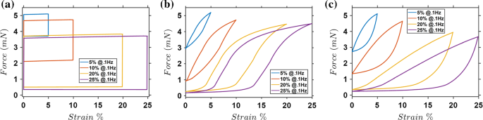

  

  Steady-state force–strain loops for a Hill-type model; b fading memory model; c modified fading memory model

• (ii) A fading memory type model based on the formulation of Hunter et al. (1998) where $\dot{\bar{\varepsilon }}$ is determined from the SF strain rate history, such that

  $$\begin{array}{*{20}c} {\dot{\bar{\varepsilon }} = \alpha \mathop \int \limits_{ - \infty }^{t} {\text{e}}^{{ - \alpha \left( {t - \tau } \right)}} \dot{\varepsilon }_{\text{sf}} {\text{d}}\tau .} \\ \end{array}$$

  (A3)

  For a constant loading and unloading strain rate magnitude, $\left| {\dot{\varepsilon }_{\text{sf}} } \right|$, $\dot{\bar{\varepsilon }}$ is given as

  $$\begin{array}{*{20}c} {\dot{\bar{\varepsilon }} = \left| {\dot{\varepsilon }_{\text{sf}} } \right|\left\{ { - {\text{e}}^{ - \alpha t} + 2{\text{e}}^{{ - \alpha \left( {t - P/2} \right)}} - 2{\text{e}}^{{ - \alpha \left( {t - P} \right)}} + 2{\text{e}}^{{ - \alpha \left( {t - 3P/2} \right)}} - 2{\text{e}}^{{ - \alpha \left( {t - 2P} \right)}} + 1} \right\} ,} \\ \end{array}$$

  (A4)

  with results shown in Fig. 11b.

• (iii) A modified fading memory type model where only shortening (negative) strain rates contribute to $\dot{\bar{\varepsilon }}$, such that

  $$\begin{array}{*{20}c} {\dot{\bar{\varepsilon }} = \alpha \mathop \int \limits_{ - \infty }^{t} {\text{e}}^{{ - \alpha \left( {t - \tau } \right)}} \dot{\varepsilon }_{\text{m}} {\text{d}}\tau ,} \\ \end{array}$$

  (A5)
  $$\begin{array}{*{20}c} {\dot{\varepsilon }_{\text{m}} = \left\{ {\begin{array}{*{20}c} {\dot{\varepsilon }_{\text{sf}} } & {\dot{\varepsilon }_{\text{sf}} \le 0} \\ 0 & {\dot{\varepsilon }_{\text{sf}} > 0} \\ \end{array} } \right. .} \\ \end{array}$$

  (A6)

  For a constant loading and unloading strain rate magnitude, $\left| {\dot{\varepsilon }_{\text{sf}} } \right|$, $\dot{\bar{\varepsilon }}$ is given as

  $$\begin{array}{*{20}c} {\dot{\bar{\varepsilon }} = \left| {\dot{\varepsilon }_{\text{sf}} } \right|\left\{ {{\text{e}}^{{ - \alpha \left( {t - P/2} \right)}} - {\text{e}}^{{ - \alpha \left( {t - P} \right)}} + {\text{e}}^{{ - \alpha \left( {t - 3P/2} \right)}} - {\text{e}}^{{ - \alpha \left( {t - 2P} \right)}} } \right\} ,} \\ \end{array}$$

  (A7)

  with results shown in Fig. 11c.

Predicted results are shown in Fig. 11a. All models approximate the following features of the experimental measurements of Wille et al.: (i) a reduction in peak tension with increasing $\varepsilon_{\max }$ and (ii) a nonzero tension at the end of each cycle for $\varepsilon_{\max }$ = 5% and 10%. However, the Hill-type model incorrectly predicts a nearly constant cell force during loading and unloading. The fading memory model predicts a transient change in force during each loading cycle, but the concave–convex curve shapes do not resemble experimental curves. The modified fading memory predicts near-linear behaviour during loading and a convex unloading curve. This is approximately similar to the experimental measurements of Wille et al.

Analyses presented in this appendix using a phenomenological modelling approach demonstrate that transient cell contractility during dynamic loading cannot be replicated using a classical Hill-type contractility mode. Fading memory approaches improve the predictions of transient force generation, and fading memory effective strain rates appear require an asymmetric between loading and unloading contributions.

In summary, the thermodynamically consistent mechanistically based cross-bridge cycling model and SF formulation presented in the main paper provides a physical rationalisation of the apparent fading memory behaviour in the experimental results of Wille et al.

Appendix B: Nonlinear viscoelastic model

Here, we provide a more detailed derivation for the nonlinear model summarised in Sect. 2.3. We consider a nonlinear Maxwell unit (nonlinear spring in series with a linear dashpot) in parallel with a second nonlinear spring. The following assumptions may be made regarding the system shown in Fig. 3:

• (i) The total stress $\sigma_{\text{cell}}^{\text{pass}} = \sigma_{nle1} + \sigma_{mw} \quad \left( {\text{B1}} \right)$,

• (ii) The total strain $\varepsilon = \varepsilon_{mw} = \varepsilon_{nle1} \quad \left( {\text{B2}} \right)$,

• (iii) $\sigma_{mw} = \sigma_{nle2} = \sigma_{\text{v}} \quad \left( {\text{B3}} \right)$,

• (iv) and $\varepsilon_{mw} = \varepsilon_{nle2} + \varepsilon_{\text{v}} \quad \left( {\text{B4}} \right)$.

Initially, let us describe the spring stress–strain relations as

$$\begin{array}{*{20}c} {\sigma_{i} = f\left( {\varepsilon_{i} } \right) = f_{i} ,\quad i = nle1, nle2} \\ \end{array}$$

(B5)

Differentiating a nonlinear elastic spring with respect to time gives

$$\begin{array}{*{20}c} {\dot{\sigma }_{nle} = \frac{\text{d}}{{{\text{d}}t}}\left( {\sigma_{nle} } \right) = \frac{{{\text{d}}f_{nle} }}{{{\text{d}}\varepsilon_{nle} }}\frac{{{\text{d}}\varepsilon_{nle} }}{{{\text{d}}t}} = \frac{{{\text{d}}f_{nle} }}{{{\text{d}}\varepsilon_{nle} }}\dot{\varepsilon }_{nle} ,} \\ \end{array}$$

(B6)

Combining with the strain (rate) constraint, we find:

$$\begin{array}{*{20}c} {\dot{\varepsilon }_{mw} = \dot{\varepsilon }_{nle2} + \dot{\varepsilon }_{\text{v}} = \frac{{\dot{\sigma }_{nle2} }}{{\frac{{{\text{d}}f_{nle2} }}{{{\text{d}}\varepsilon_{nle2} }}}} + \dot{\varepsilon }_{\text{v}} ,} \\ \end{array}$$

(B7)

so that

$$\begin{array}{*{20}c} {\frac{{{\text{d}}f_{nle2} }}{{{\text{d}}\varepsilon_{nle2} }}\dot{\varepsilon } = \dot{\sigma } + \frac{{{\text{d}}f_{nle2} }}{{{\text{d}}\varepsilon_{nle2} }}\dot{\varepsilon }_{\text{v}} .} \\ \end{array}$$

(B8)

Also, considering the stress rate:

$$\begin{array}{*{20}c} {\dot{\sigma }_{\text{cell}}^{\text{pass}} = \dot{\sigma }_{nle2} + \dot{\sigma }_{nle1} ,} \\ \end{array}$$

(B9)

so that

$$\begin{array}{*{20}c} {\dot{\sigma }_{\text{cell}}^{\text{pass}} = \frac{{{\text{d}}f_{nle2} }}{{{\text{d}}\varepsilon_{nle2} }}\dot{\varepsilon } + \frac{{{\text{d}}f_{nle1} }}{{{\text{d}}\varepsilon_{nle1} }}\dot{\varepsilon } - \frac{{{\text{d}}f_{nle1} }}{{{\text{d}}\varepsilon_{nle1} }}\dot{\varepsilon }_{\text{v}} } \\ \end{array}$$

(B10.1)

$$\begin{array}{*{20}c} { = \left( {\frac{{{\text{d}}f_{nle1} }}{{{\text{d}}\varepsilon_{nle1} }} + \frac{{{\text{d}}f_{nle2} }}{{{\text{d}}\varepsilon_{nle2} }}} \right)\dot{\varepsilon } - \frac{{{\text{d}}f_{nle2} }}{{{\text{d}}\varepsilon_{nle2} }}\dot{\varepsilon }_{\text{v}} } \\ \end{array}$$

(B10.2)

$$\begin{array}{*{20}c} { = \frac{{{\text{d}}f_{nle2} }}{{{\text{d}}\varepsilon_{nle2} }}\left( {\dot{\varepsilon } - \dot{\varepsilon }_{\text{v}} } \right) + \frac{{{\text{d}}f_{nle1} }}{{{\text{d}}\varepsilon_{nle1} }}\dot{\varepsilon }.} \\ \end{array}$$

(B10.3)

The specific form for the nonlinear spring function is given by:

$$\begin{array}{*{20}c} {\sigma_{nle} = \beta \left( {\exp \left( {\alpha \varepsilon_{nle} } \right) - 1} \right) = f_{nle} , } \\ \end{array}$$

(B11)

where $\varepsilon_{nle}$ is the strain in the spring, and $\alpha_{nle}$ and $\beta_{nle}$ (${\text{kPa}}$) are material constants. The derivative with respect to strain is then:

$$\begin{array}{*{20}c} {\frac{{{\text{d}}f_{nle} }}{{{\text{d}}\varepsilon_{nle} }} = \alpha \beta \exp \left( {\alpha \varepsilon_{nle} } \right).} \\ \end{array}$$

(B12)

The dashpot stress is:

$$\begin{array}{*{20}c} {\sigma_{\text{v}} = \xi \dot{\varepsilon }_{\text{v}} ,} \\ \end{array}$$

(B13)

where $\xi$ is the viscosity of the dashpot (${\text{kPa}}\;{\text{s}}$). Rearranging:

$$\begin{array}{*{20}c} {\dot{\varepsilon }_{\text{v}} = \frac{{\sigma_{\text{v}} }}{\xi } = \frac{1}{\xi }\left( {\sigma_{\text{vis}} - \sigma_{nle1} } \right)} \\ \end{array}$$

(B14.1)

$$\begin{array}{*{20}c} { = \frac{1}{\xi }\left( {\sigma_{\text{vis}} - \beta_{1} \left( {\exp \left( {\alpha_{1} \varepsilon } \right) - 1} \right)} \right).} \\ \end{array}$$

(B14.2)

${\text{d}}f_{nle2} /{\text{d}}\varepsilon_{nle2}$ may be arranged as:

$$\begin{array}{*{20}c} {\frac{{{\text{d}}f_{nle2} }}{{{\text{d}}\varepsilon_{nle2} }} = \alpha_{2} \beta_{2} \exp \left( {\alpha_{2} \varepsilon_{nle2} } \right)} \\ \end{array}$$

(B15.1)

$$\begin{array}{*{20}c} { = \alpha_{2} \left( {\beta_{2} + \beta_{2} \left( {\exp \left( {\alpha_{2} \varepsilon_{nle2} } \right) - 1} \right)} \right)} \\ \end{array}$$

(B15.2)

$$\begin{array}{*{20}c} { = \alpha_{2} \left( {\beta_{2} + \sigma_{nle2} } \right) = \alpha_{2} \left( {\beta_{2} + \sigma_{\text{vis}} - \sigma_{nle1} } \right)} \\ \end{array}$$

(B15.3)

$$\begin{array}{*{20}c} { = \alpha_{2} \left( {\beta_{2} + \sigma_{\text{vis}} - \beta_{1} \left( {\exp \left( {\alpha_{1} \varepsilon } \right) - 1} \right)} \right).} \\ \end{array}$$

(B15.4)

From equation B10.3, the constitutive equation for the complete viscoelastic model follows as:

$$\begin{array}{*{20}c} {\dot{\sigma }_{\text{cell}}^{\text{pass}} = \alpha_{1} \beta_{1} \exp \left( {\alpha_{1} \varepsilon } \right)\dot{\varepsilon } + \alpha_{2} \left\{ {\beta_{2} + \sigma_{\text{cell}}^{\text{pass}} - \beta_{1} \left( {\exp \left( {\alpha_{1} \varepsilon } \right) - 1} \right)} \right\}(\dot{\varepsilon } - \frac{1}{\xi }\left( {\sigma_{\text{cell}}^{\text{pass}} - \beta_{1} \left( {\exp \left( {\alpha_{1} \varepsilon } \right) - 1} \right)} \right).} \\ \end{array}$$

(B16)

References

Abercrombie M (1978) Fibroblasts. J Clin Pathol Suppl (R Coll Pathol) 12:1–6
Alberts B, Johnson A, Lewis J, Raff M, Roberts K, Walter P (2002) Molecular biology of the cell. Garland Science, New York
Balestrini JL, Billiar KL (2009) Magnitude and duration of stretch modulate fibroblast remodeling. J Biomech Eng Am Soc Mech Eng 131(5):051005. https://doi.org/10.1115/1.3049527
Chung M-W, Tsoutsman T, Semsarian C (2003) Hypertrophic cardiomyopathy: from gene defect to clinical disease. Cell Res 13(1):9–20. https://doi.org/10.1038/sj.cr.7290146
Curtin NA, Davies RE (1975) Very high tension with very little ATP breakdown by active skeletal muscle. J Mechanochem Cell Motil 3(2):147–154
Deshpande VS, McMeeking RM, Evans AG (2006) A bio-chemo-mechanical model for cell contractility. Proc Natl Acad Sci USA 103(38):14015–14020. https://doi.org/10.1073/pnas.0605837103
Deshpande VS, McMeeking RM, Evans AG (2007) A model for the contractility of the cytoskeleton including the effects of stress-fibre formation and dissociation. Proc R Soc A Math Phys Eng Sci 463(2079):787–815. https://doi.org/10.1098/rspa.2006.1793
Dowling EP, McGarry JP (2014) Influence of spreading and contractility on cell detachment. Ann Biomed Eng 42(5):1037–1048. https://doi.org/10.1007/s10439-013-0965-5
Dowling EP, Ronan W, Ofek G, Deshpande VS, McMeeking RM, Athanasiou KA, McGarry JP (2012) The effect of remodelling and contractility of the actin cytoskeleton on the shear resistance of single cells: a computational and experimental investigation. J R Soc Interface R Soc 9(77):3469–3479. https://doi.org/10.1098/rsif.2012.0428
Dowling EP, Ronan W, McGarry JP (2013) Computational investigation of in situ chondrocyte deformation and actin cytoskeleton remodelling under physiological loading. Acta Biomater 9(4):5943–5955. https://doi.org/10.1016/j.actbio.2012.12.021
Foolen J, Deshpande VS, Kanters FMWW, Baaijens FPTT (2012) The influence of matrix integrity on stress-fiber remodeling in 3D. Biomaterials 33(30):7508–7518. https://doi.org/10.1016/j.biomaterials.2012.06.103
Greaser ML, Gergely J (1971) Reconstitution of troponin activity from three protein components. J Biol Chem 246(13):4226–4233
Hara F, Fukuda K, Asada S, Matsukawa M, Hamanishi C (2001) Cyclic tensile stretch inhibition of nitric oxide release from osteoblast-like cells is both G protein and actin-dependent. J Orthop Res 19(1):126–131. https://doi.org/10.1016/S0736-0266(00)00011-5
Hill AV (1938) ‘The heat of shortening and the dynamic constants of muscle. Proc R Soc B Biol Sci 126(843):136–195. https://doi.org/10.1098/rspb.1938.0050
Hill TL (1974) ‘Theoretical formalism for the sliding filament model of contraction of striated muscle part I. Prog Biophys Mol Biol 28:267–340. https://doi.org/10.1016/0079-6107(74)90020-0
Hunter PJ, McCulloch AD, ter Keurs HEDJ (1998) Modelling the mechanical properties of cardiac muscle. Prog Biophys Mol Biol 69(2–3):289–331. https://doi.org/10.1016/S0079-6107(98)00013-3
Huxley AF (1957) Muscle structure and theories of contraction. Prog Biophys Biophys Chem 7:255–318
Huxley AF, Simmons RM (1971) Proposed mechanism of force generation in striated muscle. Nature 233(5321):533–538. https://doi.org/10.1038/233533a0
Kaunas R, Hsu, Deguchi (2010) Sarcomeric model of stretch-induced stress fiber reorganization. Cell Health Cytoskelet 3:13. https://doi.org/10.2147/CHC.S14984
Kovács M, Tóth J, Hetényi C, Málnási-Csizmadia A, Sellers JR (2004) Mechanism of blebbistatin inhibition of myosin II. J Biol Chem Am Soc Biochem Mol Biol 279(34):35557–35563. https://doi.org/10.1074/jbc.m405319200
Langanger G, Moeremans M, Daneels G, Sobieszek A, De Brabander M, De Mey J (1986) The molecular organization of myosin in stress fibers of cultured cells. J Cell Biol 102(1):200–209. https://doi.org/10.1083/jcb.102.1.200
Lessey EC, Guilluy C, Burridge K (2012) From mechanical force to RhoA activation. Biochemistry 51(38):7420–7432. https://doi.org/10.1021/bi300758e
Lucas SM, Ruff RL, Binder MD (1987) Specific tension measurements in single soleus and medial gastrocnemius muscle fibers of the cat. Exp Neurol 95(1):142–154
Lymn RW, Taylor EW (1971) Mechanism of adenosine triphosphate hydrolysis by actomyosin. Biochemistry 10(25):4617–4624
McEvoy E, Deshpande VS, McGarry P (2017) Free energy analysis of cell spreading. J Mech Behav Biomed Mater. https://doi.org/10.1016/j.jmbbm.2017.06.006
McGarry JP, Fu J, Yang MT, Chen CS, McMeeking RM, Evans AG, Deshpande VS (2009) Simulation of the contractile response of cells on an array of micro-posts. Philos Trans Ser A Math Phys Eng Sci 367(1902):3477–3497. https://doi.org/10.1098/rsta.2009.0097
McMahon TA (1984) Muscles, reflexes, and locomotion. Princeton University Press, Princeton
Mitrossilis D, Fouchard J, Guiroy A, Desprat N, Rodriguez N, Fabry B, Asnacios A (2009) Single-cell response to stiffness exhibits muscle-like behavior. Proc Natl Acad Sci USA 106(43):18243–18248. https://doi.org/10.1073/pnas.0903994106
Nieponice A, Maul TM, Cumer JM, Soletti L, Vorp DA (2007) ‘Mechanical stimulation induces morphological and phenotypic changes in bone marrow-derived progenitor cells within a three-dimensional fibrin matrix. J Biomed Mater Res, Part A 81A(3):523–530. https://doi.org/10.1002/jbm.a.31041
Obbink-Huizer C, Oomens CWJ, Loerakker S, Foolen J, Bouten CVC, Baaijens FPT (2014) Computational model predicts cell orientation in response to a range of mechanical stimuli. Biomech Model Mechanobiol 13(1):227–236. https://doi.org/10.1007/s10237-013-0501-4
Offer G, Ranatunga KW (2013) A cross-bridge cycle with two tension-generating steps simulates skeletal muscle mechanics. Biophys J 105(4):928–940. https://doi.org/10.1016/J.BPJ.2013.07.009
Pathak A, McMeeking RM, Evans AG, Deshpande VS (2011) An analysis of the cooperative mechano-sensitive feedback between intracellular signaling, focal adhesion development, and stress fiber contractility. J Appl Mech 78(4):041001. https://doi.org/10.1115/1.4003705
Pellegrin S, Mellor H, Barry P, Andrews P, Jester JV (2007) Actin stress fibres. J Cell Sci 120(Pt 20):3491–3499. https://doi.org/10.1242/jcs.018473
Rastogi K, Puliyakodan MS, Pandey V, Nath S, Elangovan R (2016) Maximum limit to the number of myosin II motors participating in processive sliding of actin. Sci Rep 6(1):32043. https://doi.org/10.1038/srep32043
Reynolds NH, McGarry JP (2015) Single cell active force generation under dynamic loading—part II: active modelling insights. Acta Biomater 27:251–263. https://doi.org/10.1016/j.actbio.2015.09.004
Reynolds NH, Ronan W, Dowling EP, Owens P, McMeeking RM, McGarry JP (2014) On the role of the actin cytoskeleton and nucleus in the biomechanical response of spread cells. Biomaterials 35(13):4015–4025. https://doi.org/10.1016/j.biomaterials.2014.01.056
Shishvan SS, Vigliotti A, Deshpande VS (2018) The homeostatic ensemble for cells. Biomech Model Mechanobiol. https://doi.org/10.1007/s10237-018-1048-1
Smith DA, Geeves MA (1995) Strain-dependent cross-bridge cycle for muscle. Biophys J 69(2):524–537. https://doi.org/10.1016/S0006-3495(95)79926-X
Smith CW, Marston SB (1985) Disassembly and reconstitution of the Ca2+-sensitive thin filaments of vascular smooth muscle. FEBS Lett 184(1):115–119
Vernerey FJ, Farsad M (2011) A constrained mixture approach to mechano-sensing and force generation in contractile cells. J Mech Behav Biomed Mater 4(8):1683–1699. https://doi.org/10.1016/J.JMBBM.2011.05.022
Vigliotti A, Ronan W, Baaijens FPT, Deshpande VS (2015) A thermodynamically motivated model for stress-fiber reorganization. Biomech Model Mechanobiol. https://doi.org/10.1007/s10237-015-0722-9
Weafer PP, Ronan W, Jarvis SP, McGarry JP (2013) Experimental and computational investigation of the role of stress fiber contractility in the resistance of osteoblasts to compression. Bull Math Biol 75(8):1284–1303. https://doi.org/10.1007/s11538-013-9812-y
Weafer PP, Reynolds NH, Jarvis SP, McGarry JP (2015) Single cell active force generation under dynamic loading—part I: AFM experiments. Acta Biomater 27:236–250. https://doi.org/10.1016/j.actbio.2015.09.006
Wille JJ, Elson EL, Okamoto RJ (2006) Cellular and matrix mechanics of bioartificial tissues during continuous cyclic stretch. Ann Biomed Eng 34(11):1678–1690. https://doi.org/10.1007/s10439-006-9153-1
Acknowledgements
Funding support was provided by the Irish Research Council (IRC) postgraduate scholarship (GOIPG/2015/2954), the National University of Ireland Galway Hardiman scholarship, and the Science Foundation Ireland (SFI-12/IP/1723). The authors would like to acknowledge the Irish Centre for High-End Computing (ICHEC) for provision of computational facilities and support.
Author information
Authors and Affiliations
Corresponding author
Additional information
Publisher’s Note
Springer Nature remains neutral with regard to jurisdictional claims in published maps and institutional affiliations.