The least dense hyperball covering of regular prism tilings in hyperbolic $n$-space

Abstract

In this paper, we study regular prism tilings and corresponding least dense hyperball coverings in $n$-dimensional hyperbolic space $\mathbb {H}^n$ $(n=3,4,5)$ by congruent hyperballs. We determine the densities of the least dense hyperball coverings, we formulate two conjectures for the candidates of the least dense hyperball coverings by congruent hyperballs in 3- and 5-dimensional hyperbolic spaces.

1 Introduction

Finding the densest (not necessarily periodic) ball packings in 3-dimensional Euclidean space is known as the Kepler Conjecture: No packing of spheres of equal radius has a density greater than the face-centred cubic packing. This density can be realized by hexagonal layers (in continuum many ways). This conjecture was first published by Johannes Kepler in his monograph The Six-Cornered Snowflake (1611). In 1953, László Fejes Tóth reduced the Kepler conjecture to an enormous calculation procedure that involved specific cases, and later suggested that computers may be helpful for solving the problem. In this way, the above four hundred year mathematical problem has finally been solved by Thomas Hales [9]. He had proved that the Kepler’s conjecture from 1611 was correct.

Ball, horoball and hyperball packings of hyperbolic spaces are extensively discussed in the literature [2, 4, 5, 8, 13–15, 18, 22] and [20]; however, there remain several open problems. Moreover, there are few results in the literature about the ball, horoball and hyperball coverings.

Ball (sphere) packing and covering problems can be generalized to the other 3-dimensional Thurston geometries, but a difficult problem is—similarly to hyperbolic space—a suitable definition of packing density. We have an extensive program in finding globally and locally optimal ball packings and least dense ball coverings in the eight Thurston geometries arising from Thurston’s geometrization conjecture (e.g. [19, 21, 24, 25]).

In this paper, we consider the hyperball covering problem in $n$-dimensional hyperbolic space.

In the hyperbolic space $\mathbb {H}^n (n \ge 3)$, a regular prism is the convex hull of two congruent $(n-1)$ dimensional regular polyhedra in ultraparallel hyperplanes, (i.e. $(n-1)$-planes), related by “translation” along the line joining their centres that is the common perpendicular of the two hyperplanes. Each vertex of such a tiling is either proper point or every vertex lies on the absolute quadric of $\mathbb {H}^n$, in which case the prism tiling is called fully asymptotic. Thus, the prism is a polyhedron having at each vertex one $(n-1)$-dimensional regular polytope and some $(n-1)$-dimensional prisms, meeting at this vertex.

From the definition of regular prism tilings and complete Coxeter orthoschemes of degree $d=1$ (see next section), it follows that a prism tiling exists in $n$-dimensional hyperbolic space $\mathbb {H}^n, (n \ge 3)$ if and only if there exists an appropriate complete Coxeter orthoscheme of degree $d=1$.

The complete Coxeter orthoschemes were classified by Im Hof in [10] by generalizing the method of Coxeter and Böhm [6]. He showed that they exist only for dimensions $\le$9. From this classification, it follows that the complete orthoschemes of degree $d=1$ exist up to 5 dimensions.

The formulas for the hyperbolic covolumes of the considered $n$-dimensional Coxeter tilings are determined in [1, 7] and [11]. Therefore, it is possible to compute the covolumes of the regular prisms and the densities of the corresponding ball, horoball and hyperball packings.

In [16] and [17], we studied regular prism tilings and corresponding optimal hyperball packings in $n$-dimensional hyperbolic space $\mathbb {H}^n$ $(n=3,4)$ and determined their metric data and their densities. In [23], we extended the method developed in the above papers to 5-dimensional regular prism tilings.

Vermes [28] proved that in the hyperbolic plane $\mathbb {H}^2$ the universal upper bound of the hypercycle packing density is $\frac{3}{\pi }$. Recently, (to the author’s best knowledge) the candidates for the densest hyperball (hypersphere) packings in 3,4 and 5-dimensional hyperbolic space $\mathbb {H}^n$ are derived from the above regular prism tilings.

In $\mathbb {H}^2$, the universal lower bound of the hypercycle covering density is $\frac{\sqrt{12}}{\pi }$ determined by Vermes in [29], but in higher dimensions there is no result on hyperball coverings and covering densities.

In this paper, we study the $n$-dimensional $(n \ge 3)$ hyperbolic regular prism honeycombs (see [16, 17, 27]) and their corresponding coverings by congruent hyperballs, and we determine their least dense covering densities. Finally, we formulate two conjectures for the candidates of the least dense hyperball coverings by congruent hyperballs in 3- and 5-dimensional hyperbolic spaces.

2 The projective model and the complete orthoschemes

For $\mathbb {H}^n$, we use the projective model in the Lorentz space $\mathbb {E}^{1,n}$ of signature $(1,n)$, i.e. $\mathbb {E}^{1,n}$ denotes the real vector space $\mathbf {V}^{n+1}$ equipped with the bilinear form of signature $(1,n)$ $\langle \mathbf {x},\mathbf {y} \rangle =-x^0y^0+x^1y^1+ \dots + x^n y^n$ where the nonzero vectors $\mathbf {x}=(x^0,x^1,\ldots ,x^n) \in \mathbf {V}^{n+1} \; \text {and} \; \mathbf {y}=(y^0,y^1,\ldots ,y^n)\in \mathbf {V}^{n+1}$, are determined up to real factors, for representing points of $\mathcal {P}^n(\mathbb {R})$. Then $\mathbb {H}^n$ can be interpreted as the interior of the quadric $Q=\{[\mathbf {x}]\in \mathcal {P}^n | \langle \mathbf {x}, \mathbf {x} \rangle =0 \}=:\partial \mathbb {H}^n$ in the real projective space $\mathcal {P}^n(\mathbf {V}^{n+1}, {\varvec{V}}_{n+1})$.

The points of the boundary $\partial \mathbb {H}^n$ in $\mathcal {P}^n$ are called points at infinity of $\mathbb {H}^n$, the points lying outside $\partial \mathbb {H}^n$ are said to be outer points of $\mathbb {H}^n$ relative to $Q$. Let $P([\mathbf {x}]) \in \mathcal {P}^n$, a point $[\mathbf {y}] \in \mathcal {P}^n$ is said to be conjugate to $[\mathbf {x}]$ relative to $Q$ if $\langle \mathbf {x}, \mathbf {y} \rangle =0$ holds. The set of all points which are conjugate to $P([\mathbf {x}])$ form a projective (polar) hyperplane $pol(P):=\{[\mathbf {y}]\in \mathcal {P}^n | \langle \mathbf {x},~\mathbf {y} \rangle =0 \}.$ Thus the quadric $Q$ induces a bijection (linear polarity $\mathbf {V}^{n+1} \rightarrow {\varvec{V}}_{n+1})$) from the points of $\mathcal {P}^n$ onto its hyperplanes.

The point $X [\mathbf{x}]$ and the hyperplane $\alpha [{\varvec{a}}]$ are called incident if $\mathbf{x}{\varvec{a}}=0$ ($\mathbf{x} \in \mathbf{V}^{n+1} \setminus \{\mathbf {0}\}, {\varvec{a}} \in {\varvec{V}}_{n+1} \setminus \{\mathbf{0}\}$).

Definition 2.1

An orthoscheme $\mathcal {S}$ in $\mathbb {H}^n (2\le n \in \mathbb {N})$ is a simplex bounded by $n+1$ hyperplanes $H^0,\ldots ,H^n$ such that (see [3, 11]) $H^i \bot H^j, \; \text {for} \; j\ne i-1,i,i+1$.

The orthoschemes of degree $d$ in $\mathbb {H}^n$ are bounded by $n+d+1$ hyperplanes $H^0,H^1,\dots ,H^{n+d}$ such that $H^i \perp H^j$ for $j \ne i-1,~i,~i+1$, where, for $d=2$, indices are taken modulo $n+3$. For a usual orthoscheme we denote the $(n+1)$-hyperface opposite to the vertex $A_i$ by $H^i$ $(0 \le i \le n)$. An orthoscheme $\mathcal {S}$ has $n$ dihedral angles which are not right angles. Let $\alpha ^{ij}$ denote the dihedral angle of $\mathcal {S}$ between the faces $H^i$ and $H^j$. Then we have $\alpha ^{ij}=\frac{\pi }{2}, \; \text {if} \; 0 \le i < j -1 \le n.$ The $n$ remaining dihedral angles $\alpha ^{i,i+1}, (0 \le i \le n-1)$ are called the essential angles of $\mathcal {S}$. Geometrically, complete orthoschemes of degree $d$ can be described as follows:

• 1. For $d=0$, they coincide with the class of classical orthoschemes introduced by Schläfli (see Definition 2.1). The initial and final vertices, $A_0$ and $A_n$ of the orthogonal edge-path $A_iA_{i+1},~ i=0,\ldots ,n-1$, are called principal vertices of the orthoscheme.

• 2. A complete orthoscheme of degree $d=1$ can be interpreted as an orthoscheme with one outer principal vertex, say $A_n$, which is truncated by its polar plane $pol(A_n)$ (see Figs. 1, 3). In this case, the orthoscheme is called simply truncated with outer vertex $A_n$.

  Fig. 1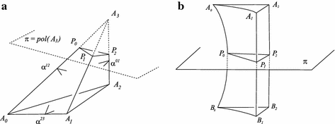

  

  a A 3-dimensional complete orthoscheme of degree $d=1$ (simple frustum orthoscheme) with outer vertex $A_3$. This orthoscheme is truncated by its polar plane $\pi =pol(A_3)$. b A part of a regular prism containing two congruent adjacent simple frustum orthoschemes

• 3. A complete orthoscheme of degree $d=2$ can be interpreted as an orthoscheme with two outer principal vertices, $A_0,~A_n$, which is truncated by its polar hyperplanes $pol(A_0)$ and $pol(A_n)$. In this case, the orthoscheme is called doubly truncated. We distinguish two different types of orthoschemes but I will not enter into the details (see [11]).

A $n$-dimensional tiling $\mathcal {P}$ (or solid tessellation, honeycomb) is an infinite set of congruent polyhedra (polytopes) that fit together to fill all space $(\mathbb {H}^n(n \geqq 2))$ exactly once, so that every face of each polyhedron (polytope) belongs to another polyhedron as well. At present, the cells are congruent orthoschemes. A tiling with orthoschemes exists if and only if each dihedral angle of a tile is submultiple of $2\pi$ (in the hyperbolic plane, the zero angle is also possible).

Another approach to describing tilings involves the analysis of their symmetry groups. If $\mathcal {P}$ is such a simplex tiling, then any motion taking one cell into another maps the entire tiling onto itself. The symmetry group of this tiling is denoted by $Sym \mathcal {P}$. Therefore, the simplex is a fundamental domain of the group $Sym \mathcal {P}$ generated by reflections in its $(n-1)$-dimensional hyperfaces.

The scheme of an orthoscheme $S$ is a weighted graph (characterizing $S\subset \mathbb {H}^n$ up to congruence) in which the nodes, numbered by $0,1,\dots ,n$ correspond to the bounding hyperplanes of $\mathcal {S}$. Two nodes are joined by an edge if the corresponding hyperplanes are not orthogonal.

For the schemes of complete Coxeter orthoschemes $\mathcal {S} \subset \mathbb {H}^n$, we adopt the usual conventions and sometimes even use them in the Coxeter case: If two nodes are related by the weight $\cos {\frac{\pi }{p}}$ then they are joined by a ($p-2$)-fold line for $p=3,4$ and by a single line marked $p$ for $p\ge 5$. In the hyperbolic case, if two bounding hyperplanes of $S$ are parallel, then the corresponding nodes are joined by a line marked $\infty$. If they are divergent, then their nodes are joined by a dotted line.

The ordered set $[k_1,\ldots ,k_{n-1},k_n]$ is said to be the Coxeter–Schl$\ddot{a}$fli symbol of the simplex tiling $\mathcal {P}$ generated by $\mathcal {S}$. To every scheme, there is a corresponding symmetric matrix $(c^{ij})$ of size $(n+1)\times (n+1)$ where $c^{ii}=1$ and, for $i \ne j\in \{0,1,2,\ldots ,n \}$, $c^{ij}$ equals ${-}\cos {\frac{\pi }{k_{ij}}}$ with all angles between the facets $i$,$j$ of $\mathcal {S}$.

For example, $(c^{ij})$ below is the so-called Coxeter–Schläfli matrix of the orthoscheme $S$ in 5-dimensional hyperbolic space $\mathbb {H}^5$ with parameters (nodes) $k_1=p,k_2=q,k_3=r,k_4=s,k_5=t$:

$$\begin{aligned} (c^{ij}):=\begin{pmatrix} 1&{}\quad -\cos {\frac{\pi }{p}}&{}\quad 0 &{}\quad 0 &{}\quad 0 &{}\quad 0\\ -\cos {\frac{\pi }{p}} &{}\quad 1 &{}\quad -\cos {\frac{\pi }{q}}&{}\quad 0 &{}\quad 0 &{}\quad 0 \\ 0 &{}\quad -\cos {\frac{\pi }{q}} &{}\quad 1 &{}\quad -\cos {\frac{\pi }{r}} &{}\quad 0 &{}\quad 0 \\ 0 &{}\quad 0 &{} -\cos {\frac{\pi }{r}} &{}\quad 1 &{}\quad -\cos {\frac{\pi }{s}} &{}\quad 0 \\ 0 &{}\quad 0 &{}\quad 0 &{}\quad -\cos {\frac{\pi }{s}} &{}\quad 1&{}\quad -\cos {\frac{\pi }{t}} \\ 0&{}\quad 0 &{}\quad 0 &{}\quad 0 &{}\quad -\cos {\frac{\pi }{t}} &{}\quad 1 \\ \end{pmatrix}. \end{aligned}$$

(2.1)

3 Regular prism tilings and their least dense hyperball coverings in $\mathbb {H}^n$

3.1 The structure of $n$-dimensional regular prism tilings

In hyperbolic space $\mathbb {H}^n$ $(n \ge 3)$, a regular prism is the convex hull of two congruent $(n-1)$ dimensional regular polyhedra in ultraparallel hyperplanes, i.e. $(n-1)$-planes, related by “translation” along the line joining their centres that is the common perpendicular of the two hyperplanes. The two regular $(n-1)$-faces of a regular prism are called cover-polytopes, and its other $(n-1)$-dimensional facets are called side-prisms.

In this section, we consider the $n$-dimensional regular prism tilings. We show that their existence is equivalent to the existence of the complete Coxeter orthoschemes of degree $d=1$ that are characterized by their Coxeter–Schläfli symbols (see Fig. 1a, b).

Remark 3.1

In $\mathbb {H}^3$ (see [16]), the corresponding prisms are called regular $p$-gonal prisms $(p \ge 3)$ in which the regular polyhedra (the cover faces) are regular $p$-gons, and the side-faces are rectangles. Figure 1b shows a part of such a prism where $A_2$ is the centre of a regular $p$-gonal face, $A_1$ is a midpoint of a side of this face, and $A_0$ is one vertex (end) of that side. Let $B_0,~B_1,~B_2$ be the corresponding points of the other $p$-gonal face of the prism.

The complete Coxeter orthoschemes were classified by Im Hof in [10] by generalizing the method of Coxeter and Böhm, who showed that they exist only for dimensions $\le 9$. From this classification, it follows that the complete orthoschemes of degree $d=1$ exist up to 5 dimensions.

• 1. In 3-dimensional hyperbolic space $\mathbb {H}^3$, the regular $p$-gonal non-uniform prism tilings $\mathcal {T}_{pqr}$ with parameters $[p,q,r]$ are the following:

  • (a) The vertex figure is either a tetrahedron, octahedron or icosahedron: $[q,r] = [3,3],~ [3,4],~[3,5]~ \Longrightarrow ~ p>6$,

  • (b) The vertex figure is a cube: $[q,r] = [4,3], ~ \Longrightarrow ~ p>4$,

  • (c) The vertex figure is a dodecahedron: $[q,r] = [5,3], ~ \Longrightarrow ~ p>3$.

Remark 3.2

In 3-dimensional hyperbolic space, there are 3 infinite series of totally asymptotic regular prism tilings. We do not consider these honeycombs in this paper because hyperball coverings cannot be derived from them.

• 2. The non-uniform compact prism tilings $\mathcal {T}_{pqrs}$ in $\mathbb {H}^4$ with parameters $[p,q,r,s]$ are the following:

  • (a) $[3,5,3,3]$ : the vertex figure of the tiling is the “120-cell”: $[q,r,s] = [5,3,3]$ and the cover faces are icosahedra $[p,q,r] =[3,5,3].$

  • (b) $[5,3,4,3]$ : the vertex figure of the tiling is “24-cell”: $[q,r,s] = [3,4,3]$ and the cover faces are dodecahedra $[p,q,r] =[5,3,4].$

Remark 3.3

The uniform compact tiling $[4,~3,~3,~5]$ in $\mathbb {H}^4$ is the regular cubic honeycomb. Here the prism is a cube and this tiling is not related to any hyperball packing. Thus, we do not consider it in this work.

• 3. The non-uniform compact prism tilings $\mathcal {T}_{pqrst}$ in $\mathbb {H}^5$ with parameters $[p,q,r,s,t]$ are the following:

  • (a) $[5,3,3,3,3]$ : the vertex figure of the tiling is: $[q,r,s,t] = [3,3,3,3]$ and the cover faces are $[p,q,r,s] =[5,3,3,3].$

  • (b) $[5,3,3,4,3]$ : the vertex figure of the tiling is: $[q,r,s,t] = [3,3,4,3]$ and the cover faces are $[p,q,r,s] =[5,3,3,4].$

  • (c) $[5,3,3,3,4]$ : the vertex figure of the tiling is: $[q,r,s,t] = [3,3,3,4]$ and the cover faces are $[p,q,r,s] =[5,3,3,3].$

• 4. There is no regular prism tiling in hyperbolic space $\mathbb {H}^n$ when $(n\ge 6)$.

Figure 2 shows a part of a 5-prism $[p,q,r,s,t]$ where $A_5$ is the outer vertex of the orthoscheme, $A_4$ is the centre of a cover-polyhedron, $A_3$ is the centre of a 3-face of the cover-polyhedron, $A_2$ is the midpoint of its 2-face, $A_1$ is a midpoint of an edge of this face, and $A_0$ is one vertex (end) of that edge ($A_0A_1A_2A_3A_4$ is a 4-dimensional hyperbolic orthoscheme see Fig. 2).

Fig. 2

A 5-dimensional complete orthoscheme of degree $d=1$ (simple frustum orthoscheme) with outer vertex $A_5$. This orthoscheme is truncated by its polar plane $\pi =pol(A_5)$. The points $P_0P_1P_2P_3P_4$ lie on the plane $\pi$ and form a 4-dimensional orthoscheme

Let $B_0,~B_1,~B_2,~B_3,B_4$ be the corresponding points of the other cover-polytope of the regular 5-prism. The midpoints of the edges $A_iB_i$ $(i\in \{0,1,2,3,4 \}$ form a hyperplane denoted by $\pi$. The foot points $P_i (i \in \{ 0,1,2,3,4 \})$ of the perpendiculars dropped from the points $A_i$ on the plane $\pi$ form the characteristic (or fundamental) simplex $P_0P_1P_2P_3P_4$ with Coxeter–Schläfli symbol $[p,q,r,s]$ (see Fig. 2) where $\pi$ is the polar hyperplane of $A_5$.

As in the 3-dimensional case, in $n$-dimensional hyperbolic space $\mathbb {H}^n$ $(n=4,5)$, it can be seen that $\mathcal {S}=A_0A_1A_2, \ldots , A_n$ $P_0P_1P_2 ,\ldots , P_n$ is an complete orthoscheme with degree $d=1$ where $A_n$ is a outer vertex of $\mathbb {H}^n$ and the points $P_0,P_1,P_2,\ldots ,P_{n-1}$ lie on its polar hyperplane $\pi$ (see Fig. 2 in 5-dimensional hyperbolic space). The corresponding regular prism $\mathcal {P}$ can be obtained by reflections on facets of $\mathcal {S}$ containing segment $A_{n-1}P_{n-1}$. We consider the images of $\mathcal {P}$ under reflections on its side facets (side-prisms). The union of these $n$-dimensional regular prisms (having the common $\pi$ hyperplane) forms an infinite polyhedron denoted by $\mathcal {F}$. $\mathcal {F}$ and its images under reflections on its “cover facets” fill hyperbolic space $\mathbb {H}^n$ without overlap and generate $n$-dimensional regular prism tilings  $\mathcal {T}$.

From the definition of the regular prism tilings and complete orthoschemes of degree $d=1$, it follows that a regular prism tiling $\mathcal {T}$ exists in $n$-dimensional hyperbolic space $\mathbb {H}^n$ where $n \ge 3$ if and only if there exists a complete Coxeter orthoscheme of degree $d=1$ with two divergent faces.

On the other hand, if an $n$-dimensional regular prism tiling $[k_1,k_2,\ldots ,k_n]$ exists, then it has to satisfy the following two requirements:

• 1. The orthogonal projection of the cover-polytope on the hyperbolic hyperplane $\pi$ is a regular Coxeter honeycomb with proper vertices and centres. Using the classical notation of the tessellations, these honeycombs are given by their Coxeter–Schläfli symbols $[k_1,\dots ,k_{n-1}]$.

• 2. The vertex figures about a vertex of such a prism tiling forms an $n$-dimensional regular polyhedron.

3.2 Volumes of the $n$-dimensional Coxeter orthoschemes

• 1. 3-dimensional hyperbolic space $\mathbb {H}^3$: Our polyhedron $A_0A_1A_2P_0P_1P_2$ is a simple frustum orthoscheme with outer vertex $A_3$ (see Fig. 1) whose volume can be calculated by the following theorem of Kellerhals [11]:

Theorem 3.4

The volume of a three-dimensional hyperbolic complete orthoscheme (except Lambert cube cases) $\mathcal {S}$ is expressed with the essential angles $\alpha _{01},\alpha _{12},\alpha _{23}, (0 \le \alpha _{ij} \le \frac{\pi }{2})$ (Fig. 1) in the following form:

$$\begin{aligned}&\hbox {Vol}_3(\mathcal {S})=\frac{1}{4} \left\{ \mathcal {L}(\alpha _{01}+\theta )-\mathcal {L}(\alpha _{01}-\theta )+\mathcal {L}\left( \frac{\pi }{2}+\alpha _{12}-\theta \right) \right. \\&\quad \left. +\mathcal {L}\left( \frac{\pi }{2}-\alpha _{12}-\theta \right) +\mathcal {L}(\alpha _{23}+\theta )- \mathcal {L}(\alpha _{23}-\theta )+2\mathcal {L}\left( \frac{\pi }{2}-\theta \right) \right\} , \end{aligned}$$

where $\theta \in [0,\frac{\pi }{2})$ is defined by the following formula:

$$\begin{aligned} \tan (\theta )=\frac{\sqrt{ \cos ^2{\alpha _{12}}-\sin ^2{\alpha _{01}} \sin ^2{\alpha _{23} }}}{\cos {\alpha _{01}}\cos {\alpha _{23}}} \end{aligned}$$

and where $\mathcal {L}(x):=-\int \limits _0^x \log \vert {2\sin {t}} \vert \hbox {d}t$ denotes the Lobachevsky function.

For our prism tilings $\mathcal {T}_{pqr}$, we have: $\alpha _{01}=\frac{\pi }{p}, \ \ \alpha _{12}=\frac{\pi }{q}, \ \ \alpha _{23}=\frac{\pi }{r}$ .

• 2. 4-dimensional hyperbolic space $\mathbb {H}^4$: The volumes $\hbox {Vol}_4(S_{pqrs})$ were determined by Kellerhals in [11]:

  $$\begin{aligned} \hbox {Vol}_4(S_{3533})=\frac{41 \pi ^2}{1{,}0800}\approx 0.03746794, \ \ \ \hbox {Vol}_4(S_{5343})=\frac{17 \pi ^2}{4{,}320}\approx 0.03883872. \end{aligned}$$

  (3.1)

• 3. 5-dimensional hyperbolic space $\mathbb {H}^5$: Kellerhals in [12] developed a procedure to determine the volumes of 5-dimensional hyperbolic orthoschemes, moreover, the volumes of the complete orthoschemes $\mathcal {S}_{pqrst}$ with Coxeter–Schläfli symbol $[5,3,3,3,3]$ and $[5,3,3,3,4]$ can be computed by the differential volume formula of Schläfli (see [7]):

  $$\begin{aligned} \hbox {Vol}_5(\mathcal {S}_{pqrst})=\frac{1}{4}\int _{\alpha _i}^{\frac{2\pi }{5}} {\hbox {Vol}_3([5,3,\beta (t)])\hbox {d}t+\frac{\zeta (3)}{3{,}200}} \end{aligned}$$

  with a compact tetrahedron $[5,3,\beta (t)]$ whose angle parameter $0<\beta (t)<\frac{\pi }{2}$ is given by

  $$\begin{aligned} \beta ({t})=\arctan {\sqrt{2-\cot ^2{t}}}. \end{aligned}$$

  Then, the volume of the 3-dimensional orthoscheme face $[5,3,\beta (t)]$ as given by Lobachevsky’s formula:

  $$\begin{aligned}&\hbox {Vol}_3([5,3,\beta (t)])=\frac{1}{4} \{\mathcal {L}_2\big (\frac{\pi }{5}+\theta (t)\big )-\mathcal {L}_2 \big (\frac{\pi }{5}-\theta (t)\big )-\mathcal {L}_2\big (\frac{\pi }{6} +\theta (t)\big )+\nonumber \\&\quad \mathcal {L}_2\big (\frac{\pi }{6}-\theta (t)\big )+\mathcal {L}_2 \big (\beta (t)+\theta (t)\big )-\mathcal {L}_2\big (\beta (t)-\theta (t)\big ) +2\mathcal {L}_2\big (\frac{\pi }{2}-\theta (t)\big ) \end{aligned}$$

  (3.2)

  where $\mathcal {L}(\omega )$ is the Lobachevsky’s function, $\theta (t)=\arctan \frac{\sqrt{1-4\sin ^2\frac{\pi }{5} \sin ^2{\beta (t)}}}{2\cos \frac{\pi }{5} \cos \beta (t)}$ and $\beta (t)=\frac{\pi }{3}$ or $\frac{\pi }{4}$.

3.3 The least dense hyperball coverings

The equidistant surface (or hypersphere) is a quadratic surface that lies at a constant distance from a plane in both halfspaces. The infinite body of the hypersphere is called a hyperball. The $n$-dimensional half-hypersphere $(n=3,4,5)$ with distance $h$ to a hyperplane $\pi$ is denoted by $\mathcal {H}_n^h$. The volume of a bounded hyperball piece $\mathcal {H}_n^h(\mathcal {A}_{n-1})$ bounded by an $(n-1)$-polytope $\mathcal {A}_{n-1} \subset \pi$, $\mathcal {H}_n^h$ and by hyperplanes orthogonal to $\pi$ derived from the facets of $\mathcal {A}_{n-1}$ can be determined by the formulas (3.3), (3.4) and (3.5) that follow from the suitable extension of the classical method of J. Bolyai:

$$\begin{aligned} \hbox {Vol}_3(\mathcal {H}_3^h(\mathcal {A}_2))&= \frac{1}{4}\hbox {Vol}_2(\mathcal {A}_{2})\left[ k \sinh \frac{2h}{k}+ 2 h \right] , \end{aligned}$$

(3.3)

$$\begin{aligned} \hbox {Vol}_4(\mathcal {H}_4^h(\mathcal {A}_3))&= \frac{1}{8} \hbox {Vol}_3(\mathcal {A}_{3})k \left[ \frac{2}{3} \sinh \frac{3h}{k}+ 6 \sinh \frac{h}{k} \right] , \end{aligned}$$

(3.4)

$$\begin{aligned} \hbox {Vol}_5(\mathcal {H}_5^h(\mathcal {A}_4))&= \frac{1}{16} \hbox {Vol}_4(\mathcal {A}_4)\left[ k\left( \frac{1}{2} \sinh \frac{4h}{k}+ 4 \sinh \frac{2h}{k}\right) +6h\right] , \end{aligned}$$

(3.5)

where the volume of the hyperbolic $(n-1)$-polytope $\mathcal {A}_{n-1}$ lying in the plane $\pi$ is $\hbox {Vol}_{n-1}(\mathcal {A}_{n-1})$. The constant $k=\sqrt{\frac{-1}{K}}$ is the natural length unit in $\mathbb {H}^n$. $K$ is set to be the constant negative sectional curvature.

We consider one of the previously described $n$-dimensional $(n=3,4,5)$ regular prism tilings $\mathcal {T}$ and the corresponding infinite polyhedron $\mathcal {F}$ derived from it (the union of $n$-dimensional regular prisms that share the common hyperplane $\pi$). $\mathcal {F}$ and its images under reflections on its “cover facets” fill hyperbolic space $\mathbb {H}^n$ without overlap.

If we start with a given congruent hyperball covering in $n$-dimensional hyperbolic space $\mathbb {H}^n$ and shrink the heights of hyperballs until they finally do not cover the space any more, then the minimal height (radius) gives the least dense covering of a given hyperball arrangement. The threshold value is called the minimal covering height (radius) of the given hyperball arrangement.

We are looking for the smallest half-hyperball ${\mathcal {H}_n^{h}}$ containing $\mathcal {F}$ with minimal covering height.

The smallest half-hypersphere $\mathcal {H}_n^h$ contains the cover faces of the regular $n$-prisms containing by $\mathcal {F}$. Therefore, the minimal distance from the $(n-1)$-midplane $\pi$ will be $h=P_0A_0>P_iA_i$ $(i\in \{1,2,3,4\}$ (Figs. 2, 3).

Fig. 3

The smallest hypersphere $\mathcal {H}_3^h$ that covers the infinite polyhedron $\mathcal {F}$ (and the cover faces which contain the triangles $A_0A_1A_2$ and $B_0B_1B_2$) with minimal covering height $h=P_0A_0>P_iA_i i \in \{1,2\}$

The smallest hypersphere $\mathcal {H}_n^h$ covers the infinite polyhedron $\mathcal {F}$ with minimal covering height, thus we obtain the locally least dense hyperball covering of the tiling $\mathcal {T}$ by the images of $\mathcal {H}_{n}^{h}$.

3.4 The computation of the minimal covering height

The points $P_0[{\mathbf {p}}_0]$ and $A_0[{\mathbf {a}}_0]$ are proper points of hyperbolic $n$-space and $P_0$ lies on the polar hyperplane $pol(A_n)[{\varvec{a}}^n]$ of the outer point $A_n$ thus

$$\begin{aligned}&\mathbf {p}_0 \sim c \cdot \mathbf {a}_n+\mathbf {a}_0 \in {\varvec{a}}^n \Leftrightarrow c \cdot \mathbf {a}_n {\varvec{a}}^n+\mathbf {a}_0 {\varvec{a}}^n=0 \Leftrightarrow c=-\frac{\mathbf {a}_0 {\varvec{a}}^n}{\mathbf {a}_n {\varvec{a}}^n} \Leftrightarrow \nonumber \\&\mathbf {p}_0 \sim -\frac{\mathbf {a}_0 {\varvec{a}}^n}{\mathbf {a}_n {\varvec{a}}^n} \mathbf {a}_n+\mathbf {a}_0 \sim \mathbf {a}_0 (\mathbf {a}_n {\varvec{a}}^n) - \mathbf {a}_n (\mathbf {a}_0 {\varvec{a}}^n)= \mathbf {a}_0 h_{nn}-\mathbf {a}_n h_{0n}, \end{aligned}$$

(3.6)

where $h_{ij}$ is the inverse of the Coxeter–Schläfli matrix $c^{ij}$ (see (2.1)) of the orthoscheme $\mathcal {S}$. The hyperbolic distance $h$ can be calculated by the following formula:

$$\begin{aligned} \cosh {P_0A_0}&= \cosh {h}=\frac{- \langle {\mathbf {p}}_0, {\mathbf {a}}_0 \rangle }{\sqrt{\langle {\mathbf {p}}_0, {\mathbf {p}}_0 \rangle \langle {\mathbf {a}}_0, {\mathbf {a}}_0 \rangle }} \nonumber \\&= \frac{h_{0n}^2-h_{00}h_{nn}}{\sqrt{h_{00}\langle \mathbf {p}_0, \mathbf {p}_0 \rangle }} = \sqrt{\frac{h_{00}~h_{nn}-h_{0n}^2}{h_{00}~h_{nn}}}. \end{aligned}$$

(3.7)

The volume of the polyhedron (complete orthoscheme of degree 1) $\mathcal {S}$ is denoted by $\hbox {Vol}_n(\mathcal {S})$.

For the density of the covering, it is sufficient to relate the volume of the minimal covering hyperball piece to that of corresponding polyhedron $\mathcal {S}$ (see Figs. 2, 3) because the tiling can be constructed of such polyhedra. This polytope and its images in $\mathcal {F}$ divide $\mathcal {H}_n^{h}$ into congruent horoball pieces whose volume is denoted by $Vol_n({\mathcal {H}_{n}^{h}(\mathcal {A}_{n-1})})$. We illustrate the 3-dimensional case of such a hyperball piece $A_0 A_1' A_2' P_0 P_1 P_2$ in Fig. 2.

The density of the least dense hyperball covering to the $n$-dimensional regular prism tiling $\mathcal {T}$ $(n=3,4,5)$ is defined by the following formula:

Definition 3.5

$$\begin{aligned} \delta ^\mathrm{min}(\mathcal {T}):=\frac{\hbox {Vol}_n(\mathcal {H}_n^h (\mathcal {A}_{n-1}))}{\hbox {Vol}_n({\mathcal {S}})}. \end{aligned}$$

(3.8)

4 The data of the hyperball coverings

• 1. 3-dimensional hyperbolic space $\mathbb {H}^3$ By formulas (3.3), (3.7), (3.8) and Theorem 3.4, we can calculate the data and the densities of the least dense hyperball coverings to each regular prism tiling in hyperbolic space $\mathbb {H}^3$. The results are summarized in Tables 1, 2, 3, 4 and 5. For each prism tiling, we determined, in a suitable interval, the graph of the functions $\hbox {Vol}_3(\mathcal {H}_3^{h})(p)$ and $\delta ^\mathrm{min}_{pqr}(p)$ as continuous functions of $p$ with fixed $q$ and $r$. In Fig. 4, we show these functions for the case $[p,~3,~3]$. From the formulas (3.7), it follows that the function $h(p)$ is decreasing and the function $\hbox {Vol}_3(\mathcal {H}_3^h)$ is increasing in its domain of definition. By Theorem 3.4 and formula (3.3), it can be seen that the function $\hbox {Vol}_3(\mathcal {S}_{pqr})(p)$ increases similarly to the function $\delta ^\mathrm{min}_{pqr}(p)$ in its domain of definition. We have depicted these functions as the continuous functions of $p$ with fixed $q=3,~r=3$, but $[p,q,r]$ provides prism tiling in $\mathbb {H}^3$ iff $p>6$ is an integer parameter. We have determined in [16] for each case the limit of the function $\hbox {Vol}_3(\mathcal {S}_{pqr})(p)$ as $p \rightarrow \infty$ (see Tables 1, 2, 3, 4, 5).

• 2. 4-dimensional hyperbolic space $\mathbb {H}^4$ We obtain the densities of the least dense hyperball covering of the regular prism tilings by the results of (3.1) and by the formulas (3.4) and (3.7) which are summarized in Table 6.

• 3. 5-dimensional hyperbolic space $\mathbb {H}^5$ The data of the least dense hyperball covering of the regular prism tilings can be determined by the formulas (3.2), (3.5) and (3.7) which are summarized in the Table 7.

Fig. 4

The functions $\hbox {Vol}_3(\mathcal {H}_3^h)(p)$ and $\delta _{pqr}^\mathrm{min}(p)$ to parameters $q=3,~r=3$

Table 1 $q=3, r=3$

Table 2 $q=4, r=3$

Table 3 $q=3, r=4$

Table 4 $q=5, r=3$

Table 5 $q=3, r=5$

Table 6 4-dimensional cases

Table 7 5-dimensional cases

Remark 4.1

In 5-dimensional hyperbolic space, there is a totally asymptotic regular prism tiling $[5,3,3,4,3]$ but we do not consider this honeycomb in this paper because no hyperball covering can be derived from it.

We formulate the following conjecture for the least dense hyperball coverings for 3 and 5 dimensional hyperbolic spaces:

Conjecture 4.1

The hyperball covering described above for Coxeter tiling $[7,3,3]$ provides the least dense hyperball covering in 3-dimensional hyperbolic space $\mathbf {H}^3$.

Conjecture 4.2

The hyperball covering described above for Coxeter tiling $[5,3,3,3,3]$ provides the least dense hyperball covering in 5-dimensional hyperbolic space $\mathbf {H}^5$.

Remark 4.2

The question of finding the densest hyperball packing and least dense hyperball covering in $n$-dimensional hyperbolic space is not settled yet, but in [26] we have developed a decomposition procedure to determine the upper bound density of the hyperball packings and the lower bound density of the hyperball coverings in hyperbolic 3-space. This decomposition procedure also confirms the above conjectures and shows that the optimal densities of packings and coverings probably belong to regular prism tilings whose vertex figures are regular tetrahedra. This is the reason why the 4-dimensional cases (probably) do not provide the least dense hyperball covering in hyperbolic 4-space.

We note here, that the discussion of the densest horoball packings in $n$-dimensional hyperbolic space $n \ge 3$ with horoballs of different types has not been settled yet either (see [14, 15, 20, 22]).

Optimal sphere packings in other homogeneous Thurston geometries represent another huge class of open mathematical problems. For these non-Euclidean geometries, only very few results are known (e.g. [19, 21, 24, 25]). Detailed studies are the objective of ongoing research. The applications of the above projective method seem to be interesting in (non-Euclidean) crystallography as well.

References

Belolipetsky, M., Emery, V.: On volumes of arithmetic quotients of \(PO(n,1), n\) odd. In: Proceedings of the London Mathematical Society (to appear, preprint). arXiv:1001.4670
Bezdek, K.: Sphere packings revisited. Eur. J. Comb. 27(6), 864–883 (2006)
Böhm, J., Hertel, E.: Polyedergeometrie in \(n\)-Dimensionalen Räumen Konstanter Krümmung. Birkhäuser, Basel (1981)
Böröczky, K.: Packing of spheres in spaces of constant curvature. Acta Math. Acad. Sci. Hung. 32, 243–261 (1978)
Böröczky, K., Florian, A.: Über die dichteste Kugelpackung im hyperbolischen Raum. Acta Math. Acad. Sci. Hung. 15, 237–245 (1964)
Coxeter, H.S.M.: Regular honeycombs in hyperbolic space. Proc. Int. Congr. Math. Amst. III, 155–169 (1954).
Emery, V., Kellerhals, R.: The three smallest compact arithmetic hyperbolic 5-orbifolds. Algebr. Geom. Topol. 13, 817–829 (2013)
Fejes Tóth, G., Kuperberg, G., Kuperberg, W.: Highly saturated packings and reduced coverings. Monatshefte für Mathematik 125(2), 127–145 (1998).
Hales, T.C.: Historical overview of the Kepler conjecture. Discrete Comput. Geom. 35, 5–20 (2006)
Im Hof, H.-C.: A class of hyperbolic Coxeter groups. Expo. Math. 3, 179–186 (1985)
Kellerhals, R.: The dilogarithm and volumes of hyperbolic polytopes. AMS Math. Surv. Monogr. 37, 301–336 (1991)
Kellerhals, R.: Volumes of hyperbolic 5-orthoschemes and the trilogarithm. Comment. Math. Helv. 67, 648–663 (1992)
Kellerhals, R.: Ball packings in spaces of constant curvature and the simplicial density function. Journal für reine und angewandte Mathematik 494, 189–203 (1998)
Kozma, R.T., Szirmai, J.: Optimally dense packings for fully asymptotic Coxeter tilings by horoballs of different types. Monatsh. Math. 168(1), 27–47 (2012)
Kozma, R.T., Szirmai, J.: New lower bound for the optimal ball packing density of hyperbolic 4-space. Discrete Comput. Geom. (2014). doi:10.1007/s00454-014-9634-1
Szirmai, J.: The \(p\)-gonal prism tilings and their optimal hypersphere packings in the hyperbolic 3-space. Acta Math. Hung. 111(1–2), 65–76 (2006)
Szirmai, J.: The regular prism tilings and their optimal hyperball packings in the hyperbolic \(n\)-space. Publ. Math. Debr. 69(1–2), 195–207 (2006)
Szirmai, J.: The optimal ball and horoball packings to the Coxeter honeycombs in the hyperbolic \(d\)-space. Beitr. Algebra Geom. 48(1), 35–47 (2007)
Szirmai, J.: The densest geodesic ball packing by a type of Nil lattices. Beitr. Algebra Geom. 48(2), 383–397 (2007)
Szirmai, J.: Horoball packings and their densities by generalized simplicial density function in the hyperbolic space. Acta Math. Hung. 136(1–2), 39–55 (2012). doi:10.1007/s10474-012-0205-8
Szirmai, J.: On lattice coverings of the Nil space by congruent geodesic balls. Mediterr. J. Math. 10(2), 953–970 (2013). doi:10.1007/s00009-012-0211-7
Szirmai, J.: Horoball packings to the totally asymptotic regular simplex in the hyperbolic \(n\)-space. Aequa. Math. 85, 471–482 (2013). doi: 10.1007/s00010-012-0158-6
Szirmai, J.: The optimal hyperball packings related to the smallest compact arithmetic 5-orbifolds (2013, submitted).
Szirmai, J.: Simply transitive geodesic ball packings to \(\mathbf{S^2\times R}\) space groups generated by glide reflections. Ann. Mat. Pur. Appl. 193(4), 1201–1211 (2014). doi: 10.1007/s10231-013-0324-z
Szirmai, J.: A candidate for the densest packing with equal balls in Thurston geometries. Beitr. Algebra Geom. 55(2), 441–452 (2014). doi:10.1007/s13366-013-0158-2
Szirmai, J.: Hyperball packings in hyperbolic 3-space. Monatsh. Math. (2014, submitted). arXiv:1405.0248
Vermes, I.: Über die Parkettierungsmöglichkeit des dreidimensionalen hyperbolischen Raumes durch kongruente Polyeder. Studia Sci. Math. Hung. 7, 267–278 (1972)
Vermes, I.: Ausfüllungen der hyperbolischen Ebene durch kongruente Hyperzykelbereiche. Raumes. Period. Math. Hung. 10(4), 217–229 (1979)
Vermes, I.: Über reguläre Überdeckungen de Bolyai-Lobatschewskischen Ebene durch kongruente Hyperzykelbereiche. Raumes. Period. Math. Hung. 25(3), 249–261 (1981)
Acknowledgments
I thank Emil Molnár for his helpful comments regarding this paper.
Author information
Authors and Affiliations
Corresponding author
Rights and permissions
About this article
Cite this article
Szirmai, J. The least dense hyperball covering of regular prism tilings in hyperbolic \(n\)-space. Annali di Matematica 195, 235–248 (2016). https://doi.org/10.1007/s10231-014-0460-0
Received:
Accepted:
Published:
Issue Date:
DOI: https://doi.org/10.1007/s10231-014-0460-0