An exponential lower bound for Zadeh’s pivot rule

Abstract

The question whether the Simplex Algorithm admits an efficient pivot rule remains one of the most important open questions in discrete optimization. While many natural, deterministic pivot rules are known to yield exponential running times, the random-facet rule was shown to have a subexponential running time. For a long time, Zadeh’s rule remained the most prominent candidate for the first deterministic pivot rule with subexponential running time. We present a lower bound construction that shows that Zadeh’s rule is in fact exponential in the worst case. Our construction is based on a close relation to the Strategy Improvement Algorithm for Parity Games and the Policy Iteration Algorithm for Markov Decision Processes, and we also obtain exponential lower bounds for Zadeh’s rule in these contexts.

1 Introduction

The quest for discovering the best pivot rule for the Simplex Algorithm [5] remains one of the most important challenges in discrete optimization. In particular, while several other weakly polynomial algorithms for solving Linear Programs have been proposed in the past [3, 9, 27,28,29], no fully “combinatorial” algorithm with strongly polynomial running time is known to date – in fact, the question whether such an algorithm exists is contained in Smale’s list of 18 mathematical problems for the century, among other famous unsolved problems like the Riemann hypothesis and the P versus NP problem [36]. The Simplex Algorithm is inherently combinatorial and may yield a strongly polynomial algorithm if a suitable pivot rule exists. The question what theoretical worst-case running time can be achieved with a pivot rule for the Simplex Algorithm is closely related to the question what the largest possible (combinatorial) diameter of a polytope is, and, in particular, to the weak Hirsch conjecture which states that the diameter is polynomially bounded [5, 35, 41].

For a variety of natural pivot rules, exponential worst-case examples were found soon after the Simplex Algorithm was proposed [1, 20, 30]. These examples are highly imbalanced in the sense that they cause some improving directions to be selected by the pivot rule only rarely, while others are selected often. Randomized pivot rules were proposed as a way to average out the behavior of the Simplex Algorithm and to thus avoid imbalanced behavior. The hope that this may lead to a better worst-case performance was met when subexponential upper bounds were eventually established for the random-facet pivot rule [22, 25, 32]. Other promising candidates for efficient pivot rules were deterministic “pseudo-random” rules that balance the behavior of the algorithm explicitly by considering all past decisions in each step, instead of obliviously deciding for improvements independently. The two most prominent examples of such pivot rules are Cunningham’s rule [4] which fixes an order of all possible improvement directions at the start and, in each step, picks the next improving direction in this order in round robin fashion, and Zadeh’s rule [43] which picks an improving direction chosen least often so far in each step. By design, bad examples are much more difficult to construct for these more balanced pivoting rules, and it took more than 30 years until the first lower bounds were established. Eventually, a subexponential lower bound was shown for the random-facet rule [17, 18, 21] and the random-edge rule [17, 33]. Most recently, a subexponential lower bound was shown for Zadeh’s rule  [7, 15], and an exponential lower bound for Cunningham’s rule [2]. An exponential lower bound for Zadeh’s rule is known on Acyclic Unique Sink Orientations [39], but it is unclear whether the corresponding construction can be realized as a Linear Program. This means that Zadeh’s rule remained the only promising candidate for a deterministic pivot rule to match the subexponential running time of the random-facet rule.

Local search algorithms similar to the Simplex Algorithm are important in other domains, like Vöge and Jurdziński’s Strategy Improvement Algorithm for Parity Games [42] and Howard’s Policy Iteration Algorithm for Markov Decision Processes [23]. Much like the Simplex Algorithm, these algorithms rely on a pivot rule that determines which local improvement to perform in each step. And much like for the Simplex Algorithm, many natural deterministic pivot rules for these algorithms have been shown to be exponential [2, 10, 12, 13], while a subexponential upper bound has been shown for the random-facet rule [16, 18, 25, 26, 32]. Again, Zadeh’s rule remained as a promising candidate for a deterministic subexponential pivot rule.

Our results and techniques. In this paper, we give the first exponential lower bound for Zadeh’s pivot rule for the Strategy Improvement Algorithm for Parity Games, for the Policy Iteration Algorithm for Markov Decision Processes, and for the Simplex Algorithm. This closes a long-standing open problem by eliminating Zadeh’s pivot rule as a candidate for a deterministic, subexponential pivot rule in each of these three areas (up to tie-breaking). We note that while the lower bound for the Simplex Algorithm is arguably our most important result, the lower bounds for Parity Games and Markov Decision Processes are important in their own right and complement previous results in these areas [10, 12, 13, 16].

Our lower bound construction is based on the technique used in [2, 15] (among others). In particular, we construct a Parity Game that forces the Strategy Improvement Algorithm to emulate a binary counter by enumerating strategies corresponding to the natural numbers 0 to $2^{n-1}$. The construction is then converted into a Markov Decision Process that behaves similarly (but not identically) regarding the Policy Iteration Algorithm. Finally, using a well-known transformation, the Markov Decision Process can be turned into a Linear Program for which the Simplex Algorithm mimics the behavior of the Policy Iteration Algorithm. We remark that we use an artificial, but systematic and polynomial time computable, tie-breaking rule for the pivot step whenever Zadeh’s rule does not yield a unique improvement direction. Importantly, while the tie-breaking rule is carefully crafted to simplify the analysis, conceptually, our construction is not based on exploiting the tie-breaking rule. Note that it cannot be avoided to fix a tie-breaking rule when analyzing Zadeh’s pivot rule, in the sense that, for every Markov Decision Process of size n, a tie-breaking rule tailored to this instance exists, such that the Policy Iteration Algorithm takes at most n steps [14,  Cor. 4.79].

Roughly speaking, much like the subexponential construction in [15], our construction consists of multiple levels, one for each bit of the counter. The subexponential construction of [15] requires each level to connect to the level of the least significant set bit of the currently represented number, which yields a quadratic number m of edges in the construction, which in turn leads to a lower bound of $2^{\varOmega (n)} = 2^{\varOmega (\sqrt{m})}$, i.e., a subexponential bound in the size $\varTheta (m)$ of the construction. In contrast, our construction only needs each level to connect to one of the first two levels, depending on whether the currently represented number is even or odd. Very roughly, this is the key idea of our result, since it allows us to reduce the size of the construction to $\varTheta (n)$, which leads to an exponential lower bound. However, to make this change possible, many other technical details have to be addressed, and, in particular, we are no longer able to carry the construction for Parity Games over as-is to Markov Decision Processes.

A challenge when constructing a lower bound for Zadeh’s rule is to keep track not only of the exact sets of improving directions in each step, but also of the exact number of times every improving direction was selected in the past. In contrast, the exponential lower bound construction for Cunningham’s rule [2] “only” needs to keep track of the next improving direction in the fixed cyclic order. As a consequence, the full proof of our result is very technical, because it requires us to consider all possible improvements in every step, and there are many transitional steps between configurations representing natural numbers. In this paper, we give an exact description of our construction and an outline of our proof. A complete and detailed proof can be found in the full version [6]. Importantly, our construction has been implemented and tested empirically for consistency with our formal treatment, see Appendix A.¹ The resulting animations of the execution for $n=3$ resp. $n=4$, which take 160 resp. 466 steps, are available online [24].

2 Parity games and strategy improvement

A Parity Game (PG) is a two player game that is played on a directed graph where every vertex has at least one outgoing edge. Formally, it is defined as a tuple $G=(V_0,V_1,E,\varOmega )$, where $V_0\cap V_1=\emptyset$, $(V_0\cup V_1,E)$ is a directed graph and $\varOmega :V_0\cup V_1\rightarrow \mathbb {N}$ is the priority function. The set $V_p$ is the set of vertices of player $p\in \{0,1\}$ and the set $E_p{:}{=}\{(v,w)\in E:v\in V_p\}$ is the set of edges of player $p\in \{0,1\}$. We let $V{:}{=}V_0\cup V_1$. A play in G is an infinite walk in the graph. The winner of a play is determined by the highest priority that occurs infinitely often along the walk. If this priority is even, player 0 wins, otherwise, player 1 wins.

Formally, a play in G can be described by a pair of strategies. A strategy for player p is a function that chooses one outgoing edge for each vertex of player p. To be precise, a (deterministic positional) strategy for player p is a function $\sigma :V_p\rightarrow V$ that selects for each vertex $v\in V_p$ a target vertex $\sigma (v)$ such that $(v,\sigma (v))\in E_p$ for all $v\in V_p$. Throughout this paper we only consider deterministic positional strategies and henceforth simply refer to them as strategies. Two strategies $\sigma ,\tau$ for players 0,1 and a starting vertex v then define a unique play starting at v with the corresponding walk being determined by the strategies of the players. A play can thus fully be described by a tuple $(\sigma ,\tau ,v)$ and is denoted by $\pi _{\sigma ,\tau ,v}$. A player 0 strategy $\sigma$ is winning for player 0 at vertex v, if player 0 is the winner of every game $\pi _{\sigma ,\tau ,v}$, regardless of $\tau$. Winning strategies for player 1 are defined analogously. A fundamental result in the theory of Parity Games is that, for every starting vertex, there always is a winning strategy for exactly one of the two players. The computational problem of solving a parity game consists in finding the corresponding partition of V.

Theorem 1

(e.g. [11, 31]) In every Parity Game, V can be partitioned into winning sets $(W_0,W_1)$, where player p has a positional winning strategy for each starting vertex $v\in W_p$.

2.1 Vertex valuations, the strategy improvement algorithm, and sink games

We now discuss the Strategy Improvement Algorithm of Vöge and Jurdziński [42] and its theoretical background. We discuss the concept of vertex valuations and define a special class of games that our construction belongs to, called sink games, and define vertex valuations for this class of games. We refer to [2, 14] for a more in-depth and general discussion of these topics.

Fix a pair $\sigma ,\tau$ of strategies for players 0,1, respectively. The idea of vertex valuations is to assign a valuation to every $v\in V$ that encodes how “profitable” vertex v is for player 0. By defining a suitable pre-order on these valuations, this enables us to compare the valuations of vertices and “improve” the strategy $\sigma$ by changing the target $\sigma (v)$ of a vertex v to a more “profitable” vertex $w\ne \sigma (v)$ with $(v,w)\in E$. Since there are only finitely many strategies and vertices, the strategy of player 0 can only be improved a finite number of times, eventually resulting in a so-called optimal strategy for player 0. It is known (e.g., [14, 42]) that an optimal strategy can then be used to determine the winning sets $W_0,W_1$ of the Parity Game and thus to solve the game.

Formally, vertex valuations are given as a totally ordered set $(U,\preceq )$. For every pair of strategies $\sigma ,\tau$, we are given a function $\varXi _{\sigma ,\tau }:V\rightarrow U$ assigning vertex valuations to vertices. Since U is totally ordered, this induces a preorder of the vertices for fixed strategies $\sigma ,\tau$. To eliminate the dependency on the player 1 strategy, we define the vertex valuation of v with respect to $\sigma$ by $\varXi _{\sigma }(v){:}{=}\min _{\prec }\varXi _{\sigma ,\tau }(v)$ where the minimum is taken over all player 1 strategies $\tau$. Formally, if $\varXi _{\sigma ,\tau }(\tau (v))\preceq \varXi _{\sigma }(v)$ for all $(v,u)\in E_1$, then the player 1 strategy $\tau$ is called counterstrategy for $\sigma$. It is well-known that counterstrategies exist and can be computed efficiently [42]. For a strategy $\sigma$, an arbitrary but fixed counterstrategy is denoted by $\tau ^{\sigma }$.

We can extend this ordering to a partial ordering of strategies by defining $\sigma \unlhd \sigma '$ if and only if $\varXi _{\sigma }(v)\preceq \varXi _{\sigma '}(v)$ for all $v\in V$. We write $\sigma \lhd \sigma '$ if $\sigma \unlhd \sigma '$ and $\sigma \ne \sigma '$. Given a strategy $\sigma$, a strategy $\sigma '$ with $\sigma \lhd \sigma '$ can be obtained by applying an improving switch. Intuitively, an improving switch is an edge such that including e in $\sigma$ improves the strategy with respect to $\unlhd$. Formally, let $e=(v,u)\in E_0$ and $\sigma (v)\ne u$. We define the strategy via if $v'\ne v$ and . The edge e is improving for $\sigma$ if and we denote the set of improving switches for $\sigma$ by $I_{\sigma }$.

The Strategy Improvement Algorithm now operates as follows. Given an initial strategy $\iota$, apply improving switches until a strategy $\sigma ^*$ with $I_{\sigma ^*}=\emptyset$ is reached. Such a strategy is called optimal and a strategy is optimal if and only if $\sigma \lhd \sigma ^*$ for all player 0 strategies [42]. The running time of this algorithm highly depends on the order in which improving switches are applied – a point that we discuss in more detail later.

This terminology allows us to introduce a special class of Parity Games, called sink games. This class allows for an easy definition of the vertex valuations as discussed after the definition.

Definition 1

A Parity Game $G=(V_0,V_1,E,\varOmega )$ together with an initial player 0 strategy $\iota$ is a Sink Game if the following two statements hold.

• 1. There is a vertex $t\in V_1$ with $(t,t)\in E$ and $\varOmega (t)=1$ reachable from all vertices. In addition, $\varOmega (v)>\varOmega (t)$ for all $v\in V{\setminus }\{t\}$. This unique vertex t is called the sink of the sink game.

• 2. For each player 0 strategy $\sigma$ with $\iota \unlhd \sigma$ and each vertex v, every play $\pi _{\sigma ,\tau ^{\sigma },v}$ ends in t.

Let $G=(V_0,V_1,E,\varOmega )$ and $\iota$ define a Sink Game. To simplify the presentation, assume that $\varOmega$ is injective. Since G is a Sink Game, every play $\pi _{\sigma ,\tau ^\sigma ,v}$ in G can be represented as the walk $\pi _{\sigma ,\tau ^\sigma ,v}=v,v_2,\dots ,v_k,(t)^{\infty }$. In particular, a play can be identified with its path component $v,v_2,\dots ,v_k$. Now, defining $\varXi _{\sigma }(v)$ as the path component of $\pi _{\sigma ,\tau ^\sigma ,v}$ is a well-studied choice of vertex valuations. To give a total ordering of the vertex valuations, it thus suffices to give a ordering of all subsets of V.

Let $M,N\subseteq V, M\ne N$. Intuitively, M is better than N for player 0 if it contains a vertex with large even priority not contained in N, or if it there is a vertex with large odd priority contained in N but not in M. Formally, $v\in M\varDelta N$ is called most significant difference of M and N if $\varOmega (v)>\varOmega (w)$ for all $w\in M\varDelta N, w\ne v$. The most significant difference of M and N is denoted by $\varDelta (M,N)$ and allows us to define an ordering $\prec$ on the subsets of V. For $M,N\subset V, M\ne N$ we define

$$\begin{aligned} N\prec M \Longleftrightarrow [\varDelta (M,N)\in M\wedge \varDelta (M,N)\text { is even}]\vee [\varDelta (M,N)\in N\wedge \varDelta (M,N)\text { is odd}]. \end{aligned}$$

Note that $\prec$ is a total ordering as we assume $\varOmega$ to be injective. We mention here that injectivity is not necessary – the most significant difference of any two vertex valuations being unique suffices.

The following theorem summarizes the most important aspects related to Parity Games, vertex valuations and improving switches. Note that the construction of vertex valuations given here is a simplified version of the general concept of vertex valuations used for Parity Games. It is, however, in accordance with the general construction and we refer to [14] for a more detailed discussion.

Theorem 2

[42] Let $G=(V_0,V_1,E,\varOmega )$ be a Sink Game and $\sigma$ be a player 0 strategy.

• 1. The vertex valuations of a player 0 strategy are polynomial-time computable.

• 2. There is an optimal player 0 strategy $\sigma ^*$ with respect to the ordering $\lhd$.

• 3. If $I_{\sigma }=\emptyset$, then $\sigma$ is optimal.

• 4. We have $I_{\sigma }=\{(v,w)\in E_0:\varXi _{\sigma }(\sigma (v))\lhd \varXi _{\sigma }(w)\}$ and for all $e\in I_{\sigma }$.

• 5. Given an optimal player 0 strategy, the winning sets $W_0$ and $W_1$ of player 0 and player 1 can be computed in polynomial time.

3 Lower bound construction

In this section, we describe a PG $S_n=(V_0,V_1,E,\varOmega )$ such that the Strategy Improvement Algorithm performs at least $2^n$ iterations when using Zadeh’s pivot rule and a specific tie-breaking rule. Before giving a formal definition, we give a high-level intuition of the main idea of the construction. A simplified visualization of the construction is given in Fig. 1.

Fig. 1

Visualization of the general structure of the binary counter for $n=4$. Level 1 encodes the least significant bit and level 4 encodes the most significant bit. The left picture shows the cycle centers and their distribution in the levels. The two figures on the right give examples for settings of the cycles representing the numbers 11 and 3, respectively

The key idea is that $S_n$ simulates an n-digit binary counter. We thus introduce notation related to binary counting. It will be convenient to consider counter configurations with more than n bits, where unused bits are zero. In particular, we always interpret bit $n+1$ as 0. Formally, we denote the set of n-bit configurations by $\mathcal {B}_n{:}{=}\{\mathfrak {b}\in \{0,1\}^{\infty }:\mathfrak {b}_i=0\quad \forall i>n\}$. We start with index one, hence a counter configuration $\mathfrak {b}\in \mathcal {B}_n$ is a tuple $(\mathfrak {b}_{n},\ldots ,\mathfrak {b}_1)$. Here, $\mathfrak {b}_1$ is the least and $\mathfrak {b}_n$ is the most significant bit. The integer value of $\mathfrak {b}\in \mathcal {B}_n$ is $\sum _{i=1}^n\mathfrak {b}_i2^{i-1}$. We identify the integer value of $\mathfrak {b}$ with its counter configuration and use the natural ordering of $\mathbb {N}$ to order counter configurations. For $\mathfrak {b}\in \mathcal {B}_n,\mathfrak {b}\ne 0$, we define $\nu (\mathfrak {b}) {:}{=}\min \{i\in \{1,\dots ,n\}:\mathfrak {b}_i = 1\}$ to be the least significant set bit of $\mathfrak {b}$.

The PG $S_n$ consists of n (nearly) identical levels and each level encodes one bit of the counter. Certain strategies and corresponding counterstrategies in $S_n$ are then interpreted as binary numbers. If the Strategy Improvement Algorithm enumerates at least one player 0 strategy per $\mathfrak {b}\in \mathcal {B}_n$ before finding the optimal strategy, it enumerates at least $2^n$ strategies. Since the game has size linear in n, this then establishes the exponential lower bound.

The main challenge is to obey Zadeh’s pivot rule as it forces the algorithm to only use improving switches used least often during the execution. Intuitively, a counter obeying this rule needs to switch bits in a “balanced” way. However, counting from 0 to $2^n-1$ in binary does not switch individual bits equally often. For example, the least significant bit is switched every time and the most significant bit is switched only once. The key idea to overcome this obstacle is to have a substructure in each level that contains two gadgets. These gadgets are called cycle centers. In every iteration of the algorithm, only one of the cycle centers is interpreted as encoding the bit of the current level. This enables us to perform operations within the other cycle center without losing the interpretation of the bit being equal to 0 or 1. This is achieved by an alternating encoding of the bit by the two cycle centers.

We now provide more details. Consider some level i, some $\mathfrak {b}\in \mathcal {B}_n$ and denote the cycle centers of level i by $F_{i,0}$ and $F_{i,1}$. One of them now encodes $\mathfrak {b}_i$. Which of them represents $\mathfrak {b}_i$ depends on $\mathfrak {b}_{i+1}$, since we always consider $F_{i,\mathfrak {b}_{i+1}}$ to encode $\mathfrak {b}_i$. This cycle center is called the active cycle center of level i, while $F_{i,1-\mathfrak {b}_{i+1}}$ is called inactive. A cycle center can additionally be closed or open. These terms are used to formalize when a bit is interpreted as 0 or 1. To be precise, $\mathfrak {b}_i$ is interpreted as 1 if and only if $F_{i,\mathfrak {b}_{i+1}}$ is closed. In this way, cycle centers encode binary numbers. Since bit $i+1$ switches every second time bit i switches, counting from 0 to $2^n-1$ in binary then results in an alternating and balanced usage of both cycle centers of any level as required by Zadeh’s pivot rule.

We now describe the construction of a parity game that implements this idea in detail. Fix some $n\in \mathbb {N}$. The vertex sets $V_0,V_1$ of the underlying graph are composed as follows:

$$\begin{aligned}&V_0\, {:}{=}\, \{b_i,g_i:i\in \{1,\dots ,n\}\} \cup \{d_{i,j,k},e_{i,j,k},s_{i,j} :i\in \{1,\dots ,n-j\}, j,k\in \{0,1\}\} \\&V_1\,{:}{=}\, \{F_{i,j} :i\in \{1,\dots , n-j\}, j\in \{0,1\}\} \cup \{h_{i,j} :i\in \{1,\dots , n-j\}, j\in \{0,1\}\}\cup \{t\} \end{aligned}$$

The priorities of the vertices and their sets of outgoing edges are given by Table 1. Note that every vertex $v\in V_0$ has at most two outgoing edges. For convenience of notation, we henceforth identify the node names $b_i$ and $g_i$ for $i > n$ with t. The graph can be separated into n levels, where the levels $i<n-1$ are structurally identical and the levels $n-1$ and n differ slightly from the other levels. The i-th level is shown in Fig. 2, the complete graph of $S_3$ is shown in Fig. 3.

Fig. 2

Level i of $S_n$ for $i\in \{1,\dots ,n-2\}$. Circular vertices are player 0 vertices, rectangular vertices are player 1 vertices. Labels below vertex names denote their priorities. Dashed vertices do not (necessarily) belong to level i

Fig. 3

The graph $S_3$ together with a canonical strategy representing the number 3 in the graph $S_3$. The dashed copies of the vertices $g_1,b_1$ and $b_2$ all refer to the corresponding vertices of levels 1 and 2. Red edges belong to the strategy of player 0, blue edges belong to the counterstrategy of player 1. The dashed edges indicate the spinal path

Table 1 Edges and vertex priorities of $S_n$

The general idea of the construction is the following. Certain pairs of player 0 strategies $\sigma$ and counterstrategies $\tau ^{\sigma }$ are interpreted as representing a number $\mathfrak {b}\in \mathcal {B}_n$. Such a pair of strategies induces a path starting at $b_1$ and ending at t, traversing the levels $i\in \{1,\dots ,n\}$ with $\mathfrak {b}_i=1$ while ignoring levels with $\mathfrak {b}_i=0$. This path is called the spinal path with respect to $\mathfrak {b}\in \mathcal {B}_n$. Ignoring and including levels in the spinal path is controlled by the entry vertex $b_i$ of each level $i\in \{1,\dots ,n\}$. To be precise, when $\mathfrak {b}$ is represented, the entry vertex of level i is intended to point towards the selector vertex $g_i$ of level i if and only if $\mathfrak {b}_i=1$. Otherwise, i.e., when $\mathfrak {b}_i=0$, level i is ignored and the entry vertex $b_i$ points towards the entry vertex of the next level.

Consider a level $i\in \{1,\dots ,n-2\}$. Attached to the selector vertex $g_i$ are the cycle centers $F_{i,0}$ and $F_{i,1}$ of level i. As described at the beginning of this section, these player 1 vertices are the main structures used for interpreting whether the bit i is equal to one. They alternate in encoding bit i. As discussed before, this is achieved by interpreting the active cycle center $F_{i,\mathfrak {b}_{i+1}}$ as encoding $\mathfrak {b}_i$ while the inactive cycle center $F_{i,1-\mathfrak {b}_{i+1}}$ does not interfere with the encoding. This enables us to manipulate the inactive part of a level without losing the encoded value of $\mathfrak {b}_i$. To this end, the selector vertex $g_i$ is used to ensure that the active cycle center is contained in the spinal path.

As discussed previously, a cycle center $F_{i,j}$ can have different configurations. To be precise, it can be closed, halfopen, or open. The configuration of $F_{i,j}$ is defined via the cycle vertices $d_{i,j,0}$ and $d_{i,j,1}$ of the cycle center and the two cycle edges $(d_{i,j,0},F_{i,j})$ and $(d_{i,j,1},F_{i,j})$. More precisely, $F_{i,j}$ is closed with respect to a player 0 strategy $\sigma$ if both cycle vertices point towards the cycle center, i.e., when $\sigma (d_{i,j,0})=\sigma (d_{i,j,1})=F_{i,j}$. If this is the case for exactly one of the two edges, the cycle center $F_{i,j}$ is called halfopen. A cycle that is neither closed nor halfopen is called open. An example of the different configurations is given in Fig. 4.

Fig. 4

A closed, a halfopen and an open cycle center. Edges of the strategy of player 0 are marked in red. Choices of player 1 are not depicted. Dots represent that the cycle vertices point to some unspecified vertex

In addition, the cycle center is connected to its upper selection vertex $s_{i,j}$. It connects the cycle center $F_{i,j}$ with the first level via $(s_{i,j},b_1)$ and with either level $i+1$ or $i+2$ via $(s_{i,j},h_{i,j})$ via the respective edge $(h_{i,0},b_{i+2})$ or $(h_{i,1},g_{i+1})$ (depending on j). This vertex is thus central in allowing $F_{i,j}$ to get access to either the beginning of the spinal path or the next level of the spinal path.

We next discuss the cycle vertices. If their cycle centers are not closed, these vertices still need to be able to access the spinal path. The valuation of vertices along this path is usually very high and it is almost always very profitable for player 0 vertices to get access to this path. Since the cycle vertices cannot obtain access via the cycle center (as this would, by definition, close the cycle center) they need to “escape” the level in another way. This is handled by the escape vertices $e_{i,j,0}$ and $e_{i,j,1}$. The escape vertices are used to connect the levels with higher indices to the first two levels and thus enable each vertex to access the spinal path. To be precise, they are connected with the entry vertex of level 2 and the selector vertex of level 1. In principle, the escape vertices will point towards $g_1$ when the least significant set bit of the currently represented number has the index 1 and towards $b_2$ otherwise.

We now formalize the idea of a strategy encoding a binary number by defining the notion of a canonical strategy. Note that the definition also includes some aspects that are purely technical, i.e., solely required for some proofs, and do not have an immediate intuitive interpretation.

Definition 2

Let $\mathfrak {b}\in \mathcal {B}_n$. A player 0 strategy $\sigma$ for the Parity Game $S_n$ is called a canonical strategy for $\mathfrak {b}$ if it has the following properties.

• 1. All escape vertices point to $g_1$ if $\mathfrak {b}_1=1$ and to $b_2$ if $\mathfrak {b}_1=0$.

• 2. The following hold for all levels $i\in \{1,\dots ,n\}$ with $\mathfrak {b}_i=1$:

  • (a) Level i needs to be accessible, i.e., $\sigma (b_i)=g_i$.

  • (b) The cycle center $F_{i,\mathfrak {b}_{i+1}}$ needs to be closed while $F_{i,1-\mathfrak {b}_{i+1}}$ must not be closed.

  • (c) The selector vertex of level i needs to select the active cycle center, i.e., $\sigma (g_i)=F_{i,\mathfrak {b}_{i+1}}$.

• 3. The following hold for all levels $i\in \{1,\dots ,n\}$ with $\mathfrak {b}_i=0$:

  • (a) Level i must not be accessible and needs to be “avoided”, i.e., $\sigma (b_i)=b_{i+1}$.

  • (b) The cycle center $F_{i,\mathfrak {b}_{i+1}}$ must not be closed.

  • (c) If the cycle center $F_{i,1-\mathfrak {b}_{i+1}}$ is closed, then $\sigma (g_i)=F_{i,1-\mathfrak {b}_{i+1}}$.

  • (d) If neither of the cycle centers $F_{i,0},F_{i,1}$ is closed, then $\sigma (g_i)=F_{i,0}$.

• 4. Let $\mathfrak {b}_{i+1}=0$. Then, level $i+1$ is not accessible from level i, i.e., $\sigma (s_{i,0})=h_{i,0}$ and $\sigma (s_{i,1})=b_1$.

• 5. Let $\mathfrak {b}_{i+1}=1$. Then, level $i+1$ is accessible from level i, i.e., $\sigma (s_{i,0})=b_1$ and $\sigma (s_{i,1})=h_{i,1}$.

• 6. If $\mathfrak {b}<2^n-1$, then both cycle centers of level $\nu (\mathfrak {b}+1)$ are open.

We use $\sigma _{\mathfrak {b}}$ to denote a canonical strategy for $\mathfrak {b}\in \mathcal {B}_n$. A canonical strategy representing (0, 1, 1) in $S_3$ is shown in Fig. 3.

As mentioned before, the main structure that is used to determine whether a bit is interpreted as being set are the cycle centers. In fact, any configuration of the cycle centers can be interpreted as an encoded number in the following way.

Definition 3

Let $\sigma$ be a player 0 strategy for $S_n$. Then, the induced bit state $\beta ^\sigma =(\beta _n^\sigma ,\dots ,\beta _1^\sigma )$ is defined inductively as follows. We define $\beta _n^{\sigma }=1$ if and only if $\sigma (d_{n,0,0})=\sigma (d_{n,0,1})=F_{n,0}$ and $\beta _i^\sigma =1$ if and only if $\sigma (d_{i,\beta _{i+1}^{\sigma },0})=\sigma (d_{i,\beta _{i+1}^{\sigma },1})=F_{i,\beta _{i+1}^{\sigma }}$ for $i<n$

This definition is in accordance with our interpretation of encoding a number as $\beta ^{\sigma _{\mathfrak {b}}}=\mathfrak {b}$ if $\sigma _{\mathfrak {b}}$ is a canonical strategy for $\mathfrak {b}$.

4 Lower bound for policy iteration on MDPs

In this section we discuss the Markov Decision Process (MDP) that is constructed analogously to the PG $S_n$. We discuss how this MDP allows the construction of a Linear Program (LP) such that the results obtained for the MDP carry over to the LP formulation. The main idea is to replace player 1 by the “random player” and to choose the probabilities in such a way that applying improving switches in the MDP behaves nearly the same way as in the PG. Note that we continue to use the same language for valuations, strategies and so on in MDP context, although other notions (like policy instead of strategy) are more common.

We give a brief introduction to the theory of MDPs (see also [2]). Similarly to a PG, an MDP is formally defined by its underlying graph $(V_0,V_R,E,r,p)$. Here, $V_0$ is the set of vertices controlled by player 0 and $V_R$ is the set of randomization vertices. We let $V{:}{=}V_0\cup V_R$. For $p\in \{0,R\}$, we define $E_{p}{:}{=}\{(v,w):v\in V_p\}$. The set $E_0$ then corresponds to possible choices that player 0 can make, and each such choice is assigned a reward by the reward function $r:E_0\rightarrow \mathbb {R}$. The set $E_R$ corresponds to probabilistic transitions and transition probabilities are specified by the function $p:E_R\rightarrow [0,1]$ with $\sum _{u:(v,u)\in E_R}p(v,u)=1$.

As for $S_n$, a (player 0) strategy is a function $\sigma :V_0\rightarrow V$ that selects for each vertex $v\in V_0$ a target corresponding to an edge, i.e., such that $(v,\sigma (v))\in E_0$. There are several computational tasks that can be investigated for MDPs. They are typically described via an objective. We consider the expected total reward objective for MDPs which can be formulated using vertex valuations in the following sense. Given an MDP, we define the vertex valuations $\varXi _{\sigma }^\mathrm {M}(*)$ with respect to a strategy $\sigma$ as the solution (if it exists) of the following set of equations:

$$\begin{aligned} \varXi _{\sigma }^\mathrm {M}(u){:}{=}{\left\{ \begin{array}{ll}r(u,\sigma (u))+\varXi _{\sigma }^\mathrm {M}(\sigma (u)), &{}u\in V_0,\\ \sum \limits _{v:(u,v)\in E_R}p(u,v)\cdot \varXi _{\sigma }^\mathrm {M}(v), &{}u\in V_R.\end{array}\right. } \end{aligned}$$

We also impose the condition that the values sum up to 0 on each irreducible recurrent class of the Markov chain defined by $\sigma$, yielding uniqueness [2]. We intentionally use very similar notation as for vertex valuations in the context of Parity Games since this allows for a unified treatment.

We now discuss the Policy Iteration Algorithm and refer to [23] for further details. Similarly to the Strategy Improvement Algorithm for PGs, this algorithm starts with some initial policy $\iota =\sigma _0$. In each step i, it generates a strategy $\sigma _i$ by changing the target vertex $\sigma _{i-1}(v)$ of some vertex $v\in V_0$ to some vertex w with $\varXi _{\sigma }^M(w)>\varXi _{\sigma }^M(\sigma _{i-1}(v))$. For an arbitrary strategy $\sigma$, such an edge $(v,w)\in E_0$ with $w\ne \sigma (v)$ but $\varXi _{\sigma }^\mathrm {M}(w)>\varXi _{\sigma }^\mathrm {M}(\sigma (v))$ is called improving switch and the set of improving switches is denoted by $I_{\sigma }$. The term optimal strategy is defined as in PG context. In particular, a strategy $\sigma$ is optimal if and only if $I_{\sigma }=\emptyset$. Moreover, applying an improving switch cannot decrease the valuation of any vertex. That is, if $e=(v,w)\in I_{\sigma }$ and denotes the strategy obtained after applying e to $\sigma$, then for all $v'\in V$ and . Since there are only finitely many strategies, the algorithm thus generates a finite sequence $\sigma _0,\sigma _1,\dots ,\sigma _N$ with $I_{\sigma _N}=\emptyset$.

We now discuss how the counter introduced in Sect. 3 is altered to obtain an MDP $M_n$. A sketch of level i of $M_n$ can be found in Fig. 5. First, all player 1 vertices are replaced by randomization vertices. This is a common technique used for obtaining MDPs that behave similarly to given PGs and was used before (e.g., [2, 10]). While the ideas used in the transformations are similar, there is no standard reduction from PGs to MDPs preserving all properties.

Fig. 5

Level i of the MDP. Circular vertices are vertices of the player, rectangular vertices are randomization vertices. Numbers below vertex names, if present, encode priorities $\varOmega$. If a vertex has priority $\varOmega (v)$, then a reward of $\langle v\rangle {:}{=}(-N)^{\varOmega (v)}$ is associated with every edge leaving this vertex

In our construction, all cycle centers $F_{i,j}$ and all vertices $h_{i,j}$ are now randomization vertices. As vertices of the type $h_{i,j}$ have only one outgoing edge, the probability of this edge is set to 1. For defining the probabilities of the cycle edges, we introduce a small parameter $\varepsilon >0$ and defer its exact definition to later. The idea is to use $\varepsilon$ to make the probabilities of edges $(F_{i,j},s_{i,j})$ very small by setting $p(F_{i,j},s_{i,j})=\varepsilon$ and $p(F_{i,j},d_{i,j,k})=\frac{1-\varepsilon }{2}$ for $k\in \{0,1\}$. Then, the valuation of $s_{i,j}$ can only contribute significantly to the valuation of $F_{i,j}$ if the cycle center is closed. If the cycle center is not closed, then the contribution of this vertex can often be neglected. However, there are situations in which even this very low contribution has a significant impact on the valuation of the cycle center. For example, if $F_{i,0}$ and $F_{i,1}$ are both open for $\sigma$, then $\varXi _{\sigma }^\mathrm {M}(F_{i,0})>\varXi _{\sigma }^\mathrm {M}(F_{i,1})$ if and only if $\varXi _{\sigma }^\mathrm {M}(s_{i,0})>\varXi _{\sigma }^\mathrm {M}(s_{i,1})$. This sometimes results in a different behavior of the MDP when compared to the PG. We discuss this later in more detail.

Second, all player 0 vertices remain player 0 vertices. Each player 0 vertex is assigned the same priority as in $S_n$. This priority is now used to define the rewards of the edges leaving a vertex. More precisely, if we denote the priority of $v\in V_0$ by $\varOmega (v)$, then we define the reward of any edge leaving v as $\langle v\rangle {:}{=}(-N)^{\varOmega (v)}$, where $N\ge 7n$ is a large and fixed parameter. Note that the reward of an edge thus only depends on its starting vertex. The reward function that is defined in that way then has the effect that vertices with an even priority are profitable while vertices with an odd priority are not profitable. In addition, the profitability of a vertex is better (resp. worse) the higher its priority is. By choosing a sufficiently large parameter N, it is also ensured that rewards are sufficiently separated. For example, the profitability of some vertex v with even priority cannot be dominated by traversing many vertices with lower but odd priorities. In principle, this ensures that the MDP behaves very similarly to the PG.

Having introduced the parameter N, we now fix the parameter $\varepsilon$ such that $\varepsilon <(N^{2n+11})^{-1}$. Note that both parameters can be encoded by a polynomial number of bits with respect to the parameter n. By defining the reward of the edge (t, t) as 0, this completely describes the MDP.

We now provide more details on the aspects where the PG and the MDP differ. One of the main differences between the PG and the MDP is the set of canonical strategies. Consider a strategy $\sigma$ representing some $\mathfrak {b}\in \mathcal {B}_n$, some level i and the two cycle centers $F_{i,0}, F_{i,1}$. In PG context, both vertices have an even priority and the priority of $F_{i,0}$ is larger than the priority of $F_{i,1}$. Thus, if both cycle centers escape the level, the valuation of $F_{i,0}$ is better than the valuation of $F_{i,1}$. Consequently, if $\sigma (g_i)\ne F_{i,0}$, then $(g_i,F_{i,0})$ is improving for $\sigma$. In some sense, this can be interpreted as the PG “preferring” $F_{i,0}$ over $F_{i,1}$. A similar, but not the same, phenomenon occurs in MDP context. If both cycle centers $F_{i,0}$ and $F_{i,1}$ are in the same “state”, then the valuation of the two upper selection vertices $s_{i,0}, s_{i,1}$ determines which cycle center has the better valuation. It turns out that the valuation of $s_{i,\mathfrak {b}_{i+1}}$ is typically better than the valuation of $s_{i,1-\mathfrak {b}_{i+1}}$. It is in particular not true that the valuation of $s_{i,0}$ is typically better than the valuation of $s_{i,1}$. Hence, the MDP “prefers” vertices $F_{i,\mathfrak {b}_{i+1}}$ over vertices $F_{i,1-\mathfrak {b}_{i+1}}$. We thus adjust the definition of a canonical strategy in MDP context in the following way.

Definition 4

Let $\mathfrak {b}\in \mathcal {B}_n$. A player 0 strategy $\sigma$ for the MDP $M_n$ is called a canonical strategy for $\mathfrak {b}$ if it has the properties defined in Definition 2 where Property 3.(d) is replaced by the following: If neither of the cycle centers $F_{i,0}, F_{i,1}$ is closed, then $\sigma (g_i)=F_{i,\mathfrak {b}_{i+1}}$.

5 Lower bound for the simplex algorithm and linear programs

Following the arguments of [2, 15], we now discuss how the MDP can be transformed into an LP such that the results obtained for the Policy Iteration Algorithm may be transferred to the Simplex Algorithm. This transformation makes use of the unichain condition. This condition (see [34]) states that the Markov Chain obtained from each strategy $\sigma$ has a single irreducible recurrent class. Unfortunately, the MDP constructed previously does not fulfill the unichain condition. As we prove in Lemma 1, it however fulfills a weak version of the unichain condition. This weak version states that the optimal policy has a single irreducible recurrent class and does not demand this to be true for every strategy. This implies that the same LP which can be obtained by transforming an MDP fulfilling the unichain condition can be used. We refer to [14, 40] for more details.

We thus return to the discussion for MDPs fulfilling the unichain condition. Optimal policies for MDPs fulfilling this condition can be found by solving the following Linear Program:

The variable x(u, v) for $(u,v)\in E_0$ represents the probability (or frequency) of using the edge (u, v). The constraints of (P) ensure that the probability of entering a vertex u is equal to the probability of exiting u. It is not difficult to see that the basic feasible solutions of (P) correspond directly to strategies of the MDP, see, e.g., [2]. For each strategy $\sigma$ we can define a feasible setting of the variables x(u, v) with $(u,v)\in E_0$ such that $x(u,v)>0$ only if $\sigma (u)=v$. Conversely, for every basic feasible solution of (P), we can define a corresponding policy $\sigma$. It is well-known that the policy corresponding to an optimal basic feasible solution of (P) is an optimal policy for the MDP (see, e.g., [2, 34]).

Our MDP only fulfills the weak unichain condition. If it is provided an initial strategy that has the same single irreducible recurrent class as the optimal policy, then the same Linear Program introduced above can be used [14]. This follows since all considered basic feasible solutions will have the same irreducible recurrent class by monotonicity. We refer to [40] for more details.

6 Lower bound proof

6.1 The approach and basic definitions

In this section we outline the proof for the exponential lower bound on the running time of the Strategy Improvement resp. Policy Iteration Algorithm using Zadeh’s pivot rule and a strategy-based tie-breaking rule. We discuss the following key components separately before combining them into our main result.² In the following, we use the notation $G_n$ to simultaneously refer to $S_n$ and $M_n$. If a statement or definition only holds for either $S_n$ or $M_n$, we explicitly state this.

• 1. We first define an initial strategy $\iota$ such that the pair $(G_n,\iota )$ defines a sink game in PG context resp. has the weak unichain condition in MDP context. We also formalize the idea of counting how often an edge has been applied as improving switch.

• 2. We then state and discuss the tie-breaking rule. Together with the initial strategy, this completely describes the application of the improving switches performed by the Strategy Improvement resp. Policy Iteration Algorithm. Further statements, proofs and explanations that are provided in Appendix C thus only serve to prove that the algorithms and the tie-breaking rule indeed behave as intended.

• 3. We then focus on a single transition from a canonical strategy $\sigma _{\mathfrak {b}}$ to the next canonical strategy $\sigma _{\mathfrak {b}+1}$. During such a transition, many improving switches need to be applied and thus many intermediate strategies need to be considered. These strategies are divided into five phases, depending on the configuration of $G_n$ induced by the encountered strategies.

• 4. To prove that the tie-breaking rule indeed proceeds along the described phases, we need to specify how often player 0 edges are applied as improving switches, which is formalized by an occurrence record. We explicitly describe the occurrence records for canonical strategies.

• 5. Finally, we combine the previous aspects to prove that applying the respective algorithms with Zadeh’s pivot rule and our tie-breaking rule yields an exponential number of iterations.

We begin by providing the initial strategy $\iota$ for $G_n$. In principle, the initial strategy is a canonical strategy for 0 in the sense of Definition 2 resp. 4.

Definition 5

The initial player 0 strategy $\iota :V_0\mapsto V$ is defined as follows:

v	$b_i (i<n)$	$b_n$	$g_i$	$d_{i,j,k}$	$e_{i,j,k}$	$s_{i,0}$	$s_{i,1} (i<n)$
$\iota (v)$	$b_{i+1}$	t	$F_{i,0}$	$e_{i,j,k}$	$b_2$	$h_{i,0}$	$b_1$

We further introduce the notion of a reachable strategy. A strategy $\sigma '$ is reachable from some strategy $\sigma$ if it can be produced by the Strategy Improvement Algorithm starting from $\sigma$ and applying a finite number of improving switches. Note that the notion of reachability does not depend on the pivot rule or the tie-breaking rule and that every strategy calculated by the Strategy Improvement resp. Policy Iteration Algorithm is reachable by definition.

Definition 6

Let $\sigma$ be a player 0 strategy for $G_n$. The set of all strategies that can be obtained from $\sigma$ by applying an arbitrary sequence of improving switches is denoted by $\varLambda _{\sigma }$. A strategy $\sigma '$ is reachable from $\sigma$ if $\sigma '\in \varLambda _{\sigma }$.

Note that reachability is a transitive property and that we include $\sigma \in \varLambda _{\sigma }$ for convenience. The i-th level of the initial strategy is shown in Fig. 6. The initial strategy is chosen such that $G_n$ and $\iota$ define a sink game in $S_n$ resp. have the weak unichain condition in $M_n$.

Fig. 6

The initial strategy $\iota$ (red edges) in level i for $i\in \{1,\dots ,n-2\}$

Lemma 1

For all $n\in \mathbb {N}$, the game $G_n$ and the initial player 0 strategy $\iota$ define a Sink Game with sink t in PG context, resp. have the weak unichain condition in MDP context.

As Zadeh’s pivot rule is a memorizing pivot rule, the algorithms need to maintain information about how often edges have been applied as improving switches. During the execution of the algorithms, we thus maintain an occurrence record $\phi ^{\sigma }:E_0\mapsto \mathbb {R}$ that specifies how often an improving switch was applied since the beginning of the algorithms. Formally, we define $\phi ^{\iota }(e)\,{:}{=}\, 0$ for every edge $e\in E_0$, i.e., the occurrence record with respect to the initial strategy is equal to 0. Then, whenever the algorithms apply an edge e, the occurrence record of e is increased by 1.

6.2 The tie-breaking rule

We now discuss the tie-breaking rule. It specifies which edge to apply if there are multiple improving switches that minimize the occurrence record for the current strategy. Note that, in contrast to many classical pivot rules, fixing a specific tie-breaking rule cannot easily be avoided for Zadeh’s pivot rule, since it is unavoidable that occurrence records occasionally coincide between multiple improving switches. Intuitively, asking for a lower bound construction to work for all tie-breaking rules might be comparably difficult to asking for a construction that works for all pivot rules in the first place.

We rely on a structurally simple tie-breaking rule that is in principle implemented as an ordering of the set $E_0$ and depends on the current strategy $\sigma$ as well as the occurrence records. In fact, it turns out to be sufficient to specify a pre-order of $E_0$ that can be extended to a total order arbitrarily. Whenever the algorithms have to break ties, they then choose the first edge according to this ordering. For convenience, there is one small exception from this behavior. During the transition from the canonical strategy representing 1 towards the canonical strategy representing 2, one improving switch e (which we do not specify yet) has to be applied earlier than during other transitions. The reason is that the occurrence records of several edges, including e, are still zero at this point in time, which leads to unwanted behavior. In later iterations, e is the unique improving switch minimizing the occurrence record whenever it has to be applied, so no special treatment is necessary.

Let $\sigma$ be a player 0 strategy for $G_n$. Henceforth, we use the symbol $*$ as a wildcard. More precisely, when using the symbol $*$, this means any suitable index or vertex (depending on the context) can be inserted for $*$ such that the corresponding edge exists. For example, the set $\{(e_{*,*,*},*)\}$ would then denote the set of all edges starting in escape vertices. Using this notation, we define the following sets of edges.

• $\mathbb {G}{:}{=}\{(g_{i},F_{i,*})\}$ is the set of all edges leaving selector vertices.

• $\mathbb {E}^0{:}{=}\{(e_{i,j,k},*):\sigma (d_{i,j,k})\ne F_{i,j}\}$ is the set of edges leaving escape vertices whose cycle vertices do not point towards their cycle center. Similarly, $\mathbb {E}^1{:}{=}\{(e_{i,j,k},*):\sigma (d_{i,j,k})=F_{i,j}\}$ is the set of edges leaving escape vertices whose cycle vertices point towards their cycle center.

• $\mathbb {D}^1{:}{=}\{(d_{*,*,*},F_{*,*})\}$ is the set of cycle edges and $\mathbb {D}^0{:}{=}\{(d_{*,*,*},e_{*,*,*})\}$ is the set of the other edges leaving cycle vertices.

• $\mathbb {B}^0{:}{=}\bigcup _{i=1}^{n-1}\{(b_i,b_{i+1})\}\cup \{(b_n,t)\}$ is the set of all edges between entry vertices. The set $\mathbb {B}^1{:}{=}\{(b_*,g_*)\}$ of all edges leaving entry vertices and entering selection vertices is defined analogously and $\mathbb {B}{:}{=}\mathbb {B}^0\cup \mathbb {B}^1$ is the set of all edges leaving entry vertices.

• $\mathbb {S}{:}{=}\{(s_{*,*},*)\}$ is the set of all edges leaving upper selection vertices.

We next define two pre-orders based on these sets. However, we need to define finer pre-orders for the sets $\mathbb {E}^0,\mathbb {E}^1,\mathbb {S}$ and $\mathbb {D}^1$ first.

Informally, the pre-order on $\mathbb {E}^0$ forces the algorithms to favor switches of higher levels and to favor $(e_{i,0,k},*)$ over $(e_{i,1,k},*)$ in $S_n$ and $(e_{i,\beta ^{\sigma }_{i+1},k},*)$ over $(e_{i,1-\beta ^{\sigma }_{i+1},k},*)$ in $M_n$. For a formal description let $(e_{i,j,x},*),(e_{k,l,y},*)\in \mathbb {E}^0$. In $S_n$, we define $(e_{i,j,x},*)\prec _\sigma (e_{k,l,y},*)$ if either $i>k$, or $i=k$ and $j<l$. In $M_n$, we define $(e_{i,j,x},*)\prec _\sigma (e_{k,l,y},*)$ if either $i>k$, or $i=k$ and $j=\beta ^{\sigma }_{i+1}$.

Similarly, the pre-order on $\mathbb {S}$ also forces the algorithm to favor switches of higher levels. Thus, for $(s_{i,j},*),(s_{k,l},*)\in \mathbb {S}$, we define $(s_{i,j},*)\prec _{\sigma } (s_{k,l},*)$ if $i>k$.

We now describe the pre-order for $\mathbb {E}^1$. Let $(e_{i,j,x},*),(e_{k,l,y},*)\in \mathbb {E}^1$.

• 1. The first criterion encodes that switches contained in higher levels are applied first. Thus, if $i>k$, then $(e_{i,j,x},*)\prec _{\sigma }(e_{k,l,y},*)$.

• 2. If $i=k$, then we consider the states of the cycle centers $F_{i,j}$ and $F_{k,l}=F_{i,1-j}$. If exactly one cycle center of level i is closed, then the improving switches within this cycle center are applied first.

• 3. Consider the case where $i=k$ but no cycle center of level i is closed. Let $t^{\rightarrow }{:}{=}b_2$ if $\nu (\mathfrak {b}+1)>1$ and $t^{\rightarrow }{:}{=}g_1$ if $\nu (\mathfrak {b}+1)=1$. If there is exactly one halfopen cycle center escaping to $t^{\rightarrow }$ in level i, then switches within this cycle center have to be applied first.

• 4. Assume that none of the prior criteria applied. This includes the case where both cycle centers are in the same state, and $i=k$ holds in this case. Then, the order of application depends on whether we consider $S_n$ or $M_n$. In $S_n$, improving switches within $F_{i,0}$ are applied first. In $M_n$, improving switches within $F_{i,\beta ^{\sigma }_{i+1}}$ are applied first.

We next give a pre-order for $\mathbb {D}_1$. Let $(d_{i,j,x},F_{i,j}),(d_{k,l,y},F_{k,l})\in \mathbb {D}^1$.

• 1. The first criterion states that improving switches that are part of open cycles are applied first. We thus define $(d_{i,j,x},F_{i,j})\prec _\sigma (d_{k,l,y},F_{k,l})$ if $\sigma (d_{k,l,1-y})=F_{k,l}$ but $\sigma (d_{i,j,1-x})\ne F_{i,j}$.

• 2. The second criterion states the following. Among all halfopen cycle centers, improving switches contained in cycle centers such that the bit of the level the cycle center is part of is equal to zero are applied first. If the first criterion does not apply, we thus define $(d_{i,j,x},F_{i,j})\prec _\sigma (d_{k,l,y},F_{k,l})$ if $\beta _k^{\sigma }>\beta _i^{\sigma }$.

• 3. The third criterion states that among all partially closed cycle centers, improving switches inside cycle centers contained in lower levels are applied first. If none of the first two criteria apply, we thus define $(d_{i,j,x},F_{i,j})\prec _\sigma (d_{k,l,y},F_{k,l})$ if $k>i$.

• 4. The fourth criterion states that improving switches within the active cycle center are applied first within one level. If none of the previous criteria apply, we thus define $(d_{i,j,x},F_{i,j})\prec _\sigma (d_{k,l,y},F_{k,l})$ if $\beta ^\sigma _{k+1}\ne l$ and $\beta ^{\sigma }_{i+1}= j$.

• 5. The last criterion states that edges with last index equal to zero are preferred within one cycle center. That is, if none of the previous criteria apply, we define $(d_{i,j,x},F_{i,j})\prec _{\sigma }(d_{k,l,y},F_{k,l})$ if $x<y$. If this criterion does not apply either, the edges are incomparable.

We now define the pre-order $\prec _{\sigma }$ and the tie-breaking rule, implemented by an ordering of $E_0$.

Definition 7

Let $\sigma$ be a player 0 strategy for $G_n$ and $\phi ^{\sigma }:E^0\rightarrow \mathbb {N}_0$ be an occurrence record. We define the pre-order $\prec _\sigma$ on $E_0$ by defining the set-based pre-order

$$\begin{aligned} \mathbb {G}\prec _\sigma \mathbb {D}^0\prec _\sigma \mathbb {E}^1\prec _\sigma \mathbb {B}\prec _\sigma \mathbb {S}\prec _\sigma \mathbb {E}^0\prec _\sigma \mathbb {D}^1 \end{aligned}$$

where the sets $\mathbb {E}^0,\mathbb {E}^1,\mathbb {S}$ and $\mathbb {D}^1$ are additionally pre-ordered as described before. We extend the pre-order to an arbitrary but fixed total ordering and denote the corresponding order also by $\prec _\sigma$. We define the following tie-breaking rule: Let $I_\sigma ^{\min }$ denote the set of improving switches with respect to $\sigma$ that minimize the occurrence record. Apply the first improving switch contained in $I_\sigma ^{\min }$ with respect to the ordering $\prec _\sigma$ with the following exception: If $\phi ^{\sigma }(b_1,b_2)=\phi ^{\sigma }(s_{1,1}, h_{1,1})=0$ and $(b_1,b_2),(s_{1,1}, h_{1,1}) \in I_\sigma$, apply $(s_{1,1}, h_{1,1})$ immediately.

We usually just use the notation $\prec$ to denote the ordering if it is clear from the context which strategy is considered and whether $\prec$ is defined via the default or special pre-order.

Lemma 2

Given a strategy $\sigma \in \varLambda _{\iota }$ and an occurrence record $\phi ^{\sigma }:E^0\rightarrow \mathbb {N}_0$, the tie-breaking rule can be evaluated in polynomial time.

6.3 The phases of a transition and the application of improving switches

As explained earlier, the goal is to prove that Zadeh’s pivot rule with our tie-breaking rule enumerates at least one strategy per number $\mathfrak {b}\in \mathcal {B}_n$. This is proven in an inductive fashion. That is, we prove that given a canonical strategy $\sigma _{\mathfrak {b}}$ for $\mathfrak {b}\in \mathcal {B}_n$, the algorithms eventually calculate a canonical strategy $\sigma _{\mathfrak {b}+1}$ for $\mathfrak {b}+1$. This process is called a transition and each transition is partitioned into up to five phases. In each phase, a different “task” is performed in order to obtain the strategy $\sigma _{\mathfrak {b}+1}$. These tasks are, for example, the opening and closing of cycle centers, updating the escape vertices or adjusting some of the selection vertices.

Fig. 7

Visualization of the phases encountered when transitioning from $\sigma _{11}$ to $\sigma _{12}$ in $S_4$. Each subfigure shows the state of the counter at the beginning of a phase. Red and green edges correspond to the strategy of player 0, blue edges to the strategy of player 1. Green edges show improving switches that were applied in the preceding phase. The edges of vertices with an outdegree of 1 are not marked as these are chosen in every strategy. All occurrences of vertices with the same label refer to the same unique vertex

Depending on whether we consider $S_n$ or $M_n$ and $\nu (\mathfrak {b}+1)$, there can be 3,4 or 5 different phases. Phases 1,3 and 5 always take place while Phase 2 only occurs if $\nu (\mathfrak {b}+1)>1$, as it updates the target vertices of some selection vertices $s_{i,j}$ with $i<\nu (\mathfrak {b}+1)$. The same holds for Phase 4, although this phase only exists if we consider $S_n$. In $M_n$, we apply the corresponding switches already in Phase 3 and there is no separate Phase 4.

We now give a detailed description of the phases. For the sake of the presentation we only describe the main function of each phase and omit switches that are applied for technical reasons. Furthermore, we abbreviate $\nu {:}{=}\nu (\mathfrak {b}+1)$ whenever $\mathfrak {b}$ is clear from the context. See Fig. 7 for a full example of the phases in a transition between two canonical strategies.

• 1. During Phase 1, cycle centers are closed such that the induced bit state of the final strategy is $\mathfrak {b}+1$. Furthermore, several cycle edges are switched such that the occurrence records of these switches are as balanced as possible. In the end of the phase, the cycle center $F_{\nu ,(\mathfrak {b}+1)_{\nu +1}}$ is closed and either Phase 2 or Phase 3 begins.

• 2. During Phase 2, the upper selection vertices $s_{i,j}$ for $i\in \{1,\dots ,\nu -1\}$ and $j=(\mathfrak {b}+1)_{i+1}$ change their targets to $h_{i,j}$. This is necessary as the induced bit state of the strategy is now equal to $\mathfrak {b}+1$. Also, the entry vertices of these levels are switched towards the entry vertex of the next level. Since $\mathfrak {b}_i=\mathfrak {b}_{i+1}$ for all $i\ne 1$ if $\nu (\mathfrak {b}+1)=1$, these operations only need to be performed if $\nu (\mathfrak {b}+1)>1$.

• 3. Phase 3 is partly responsible for applying improving switches involving escape vertices. Since $\nu (\mathfrak {b})\ne \nu (\mathfrak {b}+1)$, all escape vertices need to change their target vertices. In Phase 3, some (but not all) escape vertices perform the corresponding switch. Also, for some of these escape vertices $e_{i,j,k}$, the switch $(d_{i,j,k},e_{i,j,k})$ is applied. This later enables the application of the switch $(d_{i,j,k},F_{i,j})$ which is necessary to balance the occurrence records of the cycle edges. At the end of this phase, depending on $\nu$, either $(b_{1},g_{1})$ or $(b_1,b_2)$ is applied. In $M_n$, the switches described for Phase 4 are also applied during Phase 3.

• 4. During Phase 4, the upper selection vertices $s_{i,j}$ for $i\in \{1,\dots ,\nu -1\}$ and $j\ne (\mathfrak {b}+1)_{i+1}$ change their targets to $b_1$. Updating the upper selection vertices is necessary since they need to give their cycle centers access to the spinal path. Similar to Phase 2, these switches are only performed if $\nu (\mathfrak {b}+1)>1$.

• 5. During Phase 5, the remaining escape vertices switch their targets and some of the cycle vertices switch to their cycle centers. This phase ends once all improving switches at the escape vertices are performed, yielding a canonical strategy for $\mathfrak {b}+1$.

We next give the formal definition of the different phases. For this, we need to introduce a strategy-based parameter $\mu ^{\sigma }\in \{1,\dots ,n+1\}$. This parameter $\mu ^{\sigma }$ is called the next relevant bit of the strategy $\sigma$. Before defining this parameter formally, we briefly explain its importance and how it can be interpreted.

As described in Sect. 3, both cycle centers of level i alternate in encoding bit i. Therefore, the selection vertex $g_i$ needs to select the correct cycle center and the entry vertex $b_i$ should point towards $g_i$ if and only if bit i is equal to one (see Definition 2). In particular, the selection vertex $g_{i-1}$ of level $i-1$ needs to be in accordance with the entry vertex $b_i$ of level i if bit $i-1$ is equal to one. That is, it should not happen that $\sigma (b_i)=g_i$ and $\sigma (b_{i+1})=g_{i+1}$ but $\sigma (g_{i})=F_{i,0}$. However, we cannot guarantee that this does not happen for some intermediate strategies. Therefore, we need to perform some operations within the levels i and $i-1$ and define $\mu ^{\sigma }$ as the lowest level higher than any level that is set “incorrectly” in that sense. If there are no such levels, the parameter denotes the index of the lowest level with $\sigma (b_i)=b_{i+1}$. The parameter can thus be interpreted as an indicator encoding where “work needs to be done next". As its formal definition is rather complex, we introduce an additional notation ${\bar{\sigma }}$ that somehow "encodes" $\sigma$ using integer numbers. As this notation is however a pure formal tool, we do not fully introduce it here. The definition is provided in Appendix B. Formally, the next relevant bit is now defined as follows.

Definition 8

Let $\sigma \in \varLambda _{\iota }$. The set $\mathfrak {I}^{\sigma }{:}{=}\{i\in \{1,\dots ,n\}:{\bar{\sigma }}(b_{i})\wedge {\bar{\sigma }}(g_{i})\ne {\bar{\sigma }}(b_{i+1})\}$ is the set of incorrect levels. The next relevant bit $\mu ^{\sigma }$ of the strategy $\sigma$ is defined by

$$\begin{aligned} \mu ^{\sigma }{:}{=}{\left\{ \begin{array}{ll} \min (\{n\}\cup \{i'>\max \{i\in \mathfrak {I}^{\sigma }\}:{\bar{\sigma }}(b_{i'})\wedge {\bar{\sigma }}(g_{i'})={\bar{\sigma }}(b_{i'+1})\}) &{}\text {if }\mathfrak {I}^{\sigma }\ne \emptyset , \\ \min (\{i\in \{1,\dots ,n+1\}:\sigma (b_{i})=b_{i+1}\}) &{}\text {if }\mathfrak {I}^{\sigma }=\emptyset . \end{array}\right. } \end{aligned}$$

Note that we interpret expressions of the form $x\wedge y=z$ as $x\wedge (y=z)$. Using the next relevant bit $\mu ^{\sigma }$, we now give a formal definition of the phases. Formally, a strategy belongs to one of the five phases if it has a certain set of properties. These properties can be partitioned into several categories and are described in Table 5 in Appendix B. Each of these properties depends on either the level or the cycle center. Properties Bac1, Bac2 and Bac3 involve the entry vertices ${{\varvec{b}}}$, Properties Usv1 and Usv2 involve the Upper Selection Vertices and Properties Esc1, Esc2, Esc3, Esc4 and Esc5 the Escape vertices. In addition, Properties Rel1 and Rel2 involve the next relevant bit $\mu ^{\sigma }$, Properties Cc1, Cc2 the Cycle Centers and Property Sv1 the Selection Vertices.

For most of the phases, there are additional special conditions that need to be fulfilled. The corresponding conditions simplify the distinction between different phases and allow for an easier argumentation or description of statements. However, we do not discuss these here as they are solely needed for technical reasons and we refer to Appendix B for details. We also provide the table used for the exact definition of the phases there.

Definition 9

(Phase-k -strategy) Let $\mathfrak {b}\in \mathcal {B}_n, \sigma \in \varLambda _{\iota }$ and $k\in \{1,\dots ,5\}$. The strategy $\sigma$ is a Phase-k-strategy for $\mathfrak {b}$ if it has the properties of the k-th column of Table 4 for the respective indices as well as the special conditions of the respective phase (if there are any).

6.4 The occurrence records

We next describe the actual occurrence records that occur when applying the Strategy Improvement resp. Policy Iteration Algorithm. To do so, we need to introduce notation related to binary counting.

The number of applications of specific edges in level i as improving switches depends on the last time the corresponding cycle centers were closed or how often they were closed. We thus define as the number of numbers smaller than $\mathfrak {b}$ with least significant set bit having index i. To quantify how often a specific cycle center was closed, we introduce the maximal flip number and the maximal unflip number. Let $\mathfrak {b}\in \mathcal {B}_n, i\in \{1,\dots ,n\}$ and $j\in \{0,1\}$. Then, we define the maximal flip number as the largest $\tilde{\mathfrak {b}}\le \mathfrak {b}$ with $\nu (\tilde{\mathfrak {b}})=i$ and $\tilde{\mathfrak {b}}_{i+1}=j$. Similarly, we define the maximal unflip number as the largest $\tilde{\mathfrak {b}}\le \mathfrak {b}$ with $\tilde{\mathfrak {b}}_1=\dots =\tilde{\mathfrak {b}}_i=0$ and $\tilde{\mathfrak {b}}_{i+1}=j$. If there are no such numbers, then . If we do not impose the condition that bit $i+1$ needs to be equal to j then we omit the term in the notation., i.e., and $\mathrm {mufn}(\mathfrak {b},i)$ is defined analogously.

These notations enable us to properly describe the occurrence records. We however do not describe the occurrence record for every strategy $\sigma$ produced by the considered algorithms. Instead, we only give a description of the occurrence records for canonical strategies. When discussing the application of the improving switches, we later prove the following: Assuming that the occurrence records are described correctly for $\sigma _{\mathfrak {b}}$, they are also described correctly for $\sigma _{\mathfrak {b}+1}$ when improving switches are applied according to Zadeh’s pivot rule and our tie-breaking rule.

Table 2 Occurrence records for the canonical strategy $\sigma _{\mathfrak {b}}$

Theorem 3

Let $\sigma _{\mathfrak {b}}$ be a canonical strategy for $\mathfrak {b}\in \mathcal {B}_n$ and assume that improving switches are applied as described in Sect. 6.3. Then Table 2 describes the occurrence records with respect to $\sigma _{\mathfrak {b}}$.

We now give some intuition for the occurrence records of parts of Table 2. As the occurrence records of most of the edges are much more complicated to explain, we omit an intuitive description of their occurrence records here. Let $\sigma _{\mathfrak {b}}\in \varLambda _{\iota }$ be a canonical strategy for $\mathfrak {b}\in \mathcal {B}_n$.

Consider some edge $(b_i,g_i)$. This edge is applied as an improving switch whenever bit i switches from 0 to 1. That is, it is applied if and only if we transition towards some $\mathfrak {b}'\in \mathcal {B}_n$ with $\nu (\mathfrak {b}')=i$ and $\mathfrak {b}'\le \mathfrak {b}$. Therefore, . Now consider $(b_i,b_{i+1})$. This edge is only applied as an improving switch when bit i switches from 1 to 0. This can however only happen if bit i switched from 0 to 1 earlier. That is, applying $(b_i,b_{i+1})$ can only happen when $(b_i,g_i)$ was applied before. Also, we can only apply the switch $(b_i,g_i)$ again after bit i has been switched back to 0 again, i.e., after $(b_i,b_{i+1})$ was applied. Consequently, .

Next, consider some edge $(s_{i,j},h_{i,j})$ and fix $j=1$ for now. This edge is applied as an improving switch if and only if bit $i+1$ switches from 0 to 1. Hence, as discussed before, . Now let $j=0$. The switch $(s_{i,0},h_{i,0})$ is applied whenever bit $i+1$ switches from 1 to 0. This requires the bit to have switched from 0 to 1 before. Therefore, . Further note that the switch $(s_{i,j},b_1)$ is applied in the same transitions in which the switch $(s_{i,1-j},h_{i,1-j})$ is applied. Hence, and .

Finally consider some edge $(e_{i,j,k},g_1)$. This edge is applied as an improving switch whenever the first bit switches from 0 to 1. Since 0 is even, this happens once for every odd number smaller than or equal to $\mathfrak {b}$, i.e., $\left\lceil \frac{\mathfrak {b}}{2}\right\rceil$ times. Since the switch $(e_{i,j,k},b_2)$ is applied during each transition in which the switch $(e_{i,j,k},g_1)$ is not applied, we have $\phi (e_{i,j,k},g_1)=\mathfrak {b}-\left\lceil \frac{\mathfrak {b}}{2}\right\rceil = \left\lfloor \frac{\mathfrak {b}}{2}\right\rfloor$ as $\mathfrak {b}\in \mathbb {N}$.

6.5 Proving the lower bound

We now sketch our proof that applying the Strategy Improvement resp. Policy Iteration Algorithm with Zadeh’s pivot rule and our tie-breaking rule introduced in Definition 7 takes an exponential number of iterations. This is shown in an inductive fashion as follows. Assume that we are given a canonical strategy $\sigma _{\mathfrak {b}}$ for some $\mathfrak {b}\in \mathcal {B}_n$ that fulfills a certain set of conditions. Then, applying improving switches according to Zadeh’s pivot rule and our tie-breaking rule produces a canonical strategy $\sigma _{\mathfrak {b}+1}$ for $\mathfrak {b}+1$ that fulfills the same conditions. If we can then show that the initial strategy $\iota$ is a canonical strategy for 0 having the desired properties, our bound on the number of iterations follows. Most of these properties are however rather complicated and are only needed for technical reasons. We thus do not discuss them here and refer to Appendix B for a detailed overview. These conditions are called canonical conditions and are the following:

• 1. The occurrence records $\phi ^{\sigma _{\mathfrak {b}}}$ are described correctly by Table 2.

• 2. $\sigma _{\mathfrak {b}}$ has Properties (Or1)$_{*,*,*}$ to (Or4)$_{*,*,*}$ related to the occurrence records.

• 3. Any improving switch was applied at most once per previous transition.

As a basis for the following proofs and statements, we give a characterization of the set of improving switches for canonical strategies. We furthermore prove that canonical strategies are Phase-1-strategies for the corresponding number. We use the notation $\sigma \rightarrow \sigma '$ to denote the sequence of strategies calculated by the algorithms when starting with $\sigma$ until they eventually reach $\sigma '$. Throughout this section let $\nu \, {:}{=}\,\nu (\mathfrak {b}+1)$.

Lemma 3

Let $\sigma _{\mathfrak {b}}\in \varLambda _{\iota }$ be a canonical strategy for $\mathfrak {b}\in \mathcal {B}_n$. Then $\sigma _{\mathfrak {b}}$ is a Phase-1-strategy for $\mathfrak {b}$ and $I_{\sigma _{\mathfrak {b}}}=\{(d_{i,j,k},F_{i,j}):\sigma _{\mathfrak {b}}(d_{i,j,k})\ne F_{i,j}\}$.

As claimed, $\iota$ is in fact a canonical strategy and fulfills the canonical conditions.

Lemma 4

The initial strategy $\iota$ is a canonical strategy for 0 fulfilling the canonical conditions.

We now discuss how the main statement is proven. Consider some canonical strategy $\sigma _{\mathfrak {b}}$ for some $\mathfrak {b}\in ~\mathcal {B}_n$. We prove that applying improving switches to $\sigma _{\mathfrak {b}}$ using Zadeh’s pivot rule and our tie-breaking rule produces a specific Phase-k-strategy for $\mathfrak {b}$ for every $k~\in ~\{1,\dots ,5\}$. These strategies are typically the first strategy of the corresponding phase and have several nice properties that help in proving the statement. The properties of these strategies and the set of improving switches of these strategies are summarized in Tables 6 and 7 in Appendix B. We finally prove that applying improving switches to the Phase-5-strategy that is calculated by the Strategy Improvement resp. Policy Iteration Algorithm then yields a canonical strategy $\sigma _{\mathfrak {b}+1}$ for $\mathfrak {b}+1$ fulfilling the canonical conditions. Since $\iota$ is a canonical strategy for 0 fulfilling the canonical conditions, we can then apply the statement iteratively to prove the main theorem of this paper.

Before formally stating this idea as a theorem, we discuss the individual phases. Consider Phase 1. In this phase, (mainly) cycle edges $(d_{i,j,k},F_{i,j})$ are applied. The last switch of this phase closes the cycle center $F_{\nu ,(\mathfrak {b}+1)_{\nu +1}}$. We will show that after the application of this switch, the induced bit state of the strategy is $\mathfrak {b}+1$. As a consequence, the resulting strategy is not a Phase-1-strategy. It then depends on the parity of $\mathfrak {b}$ whether this strategy belongs to Phase 2 or Phase 3. If $\nu >1$, then the next strategy is a Phase 2 strategy. If $\nu =1$, then the next strategy is a Phase-3-strategy.

Now consider the beginning of Phase 2. The properties of the corresponding strategy we refer to here are given by Tables 6 and 7. Since the induced bit state of the strategy changed from $\mathfrak {b}$ to $\mathfrak {b}+1$, the entry vertices of all levels $i\le \nu$ need to be adjusted. Accordingly, the upper selection vertices of all levels $i<\nu$ need to be adjusted. This is reflected by the set of improving switches, containing the edges $(b_{\nu },g_{\nu })$ and $(s_{\nu -1,1}, h_{\nu -1,1})$. Moreover, edges $(d_{*,*,*},F_{*,*})$ that were improving for $\sigma _{\mathfrak {b}}$ and have not been applied yet remain improving and these edges have relatively high occurrence records. Also, Table 2 describes the occurrence records of the edges that were just applied when interpreted for $\mathfrak {b}+1$. Note that we explicitly exclude the switches $(g_i,F_{i,j})$ here. The reason is that it is hard to show that the bound on the occurrence records of these edges is valid by only considering a single transition. We will thus show that these switches cannot be applied too often during $\iota \rightarrow \sigma _{\mathfrak {b}}$ for any $\mathfrak {b}\in \mathcal {B}_n$ after discussing the single phases is detail.

As discussed previously, the targets of the upper selection vertices are not set correctly for $\mathfrak {b}+1$ if $\nu >1$. This is partly handled during Phase 2. More precisely, the improving switches $(s_{i,(\mathfrak {b}+1)_{i+1}},h_{i,(\mathfrak {b}+1)_{i+1}})$ are applied during Phase 2 for all $i<\nu$. Furthermore, the target vertices of all entry vertices $b_2$ to $b_\nu$ are updated during Phase 2. After applying all of these switches, we then have a Phase-3-strategy. Since none of these switches needs to be applied if $\nu =1$, we reach such a Phase-3-strategy directly after Phase 1 in that case.

The Phase 3 strategy obtained at this point shares several properties with the Phase 2 strategy described earlier. For example, if $(d_{*,*,*}, F_{*,*})$ was improving for $\sigma _{\mathfrak {b}}$, it is still improving at the beginning of Phase 3 and has a “high” occurrence record. Furthermore, all edges $(e_{*,*,*}, b_2)$ resp. $(e_{*,*,*}, g_1)$ are improving now. The explanation for this is that the spinal path already contains the correct levels with respect to $\mathfrak {b}+1$ (with the exception of the corresponding edge starting at $b_1$) and has thus a very good valuation. Note that this requires that the vertices $s_{i,(\mathfrak {b}+1)_{i+1}}$ were updated for $i<\nu$. The vertices $b_2$ resp. $g_1$ are thus very profitable, implying that all edges leading directly towards these vertices become improving.

It turns out that switches $(e_{*,*,*},*)$ then minimize the occurrence record and are applied next. Due to the tie-breaking rule, the algorithms then only apply switches $(e_{i,j,k},*)$ with $\sigma (d_{i,j,k})=F_{i,j}$. If $(\mathfrak {b}+1)_i\ne 1$ or $(\mathfrak {b}+1)_{i+1}\ne j$, applying a switch $(e_{i,j,k},*)$ can then make the edge $(d_{i,j,k},e_{i,j,k})$ improving. However, the occurrence record of these edges is bounded from above by the occurrence record of the just applied switch $(e_{i,j,k},*)$. Consequently, such a switch is then applied next.

At this point, there is a major difference between $S_n$ and $M_n$. In $S_n$, the application of such a switch has no influence on the valuation of the corresponding cycle center $F_{i,j}$. The reason is that the player 1 controlled cycle center can simply choose the other cycle vertex (or, in case that the cycle center was closed, $s_{i,j}$). This is not true in $M_n$ as the valuation of $F_{i,j}$ is then directly affected if the valuation of the cycle vertices changes. Thus, the valuation of cycle centers increases in $M_n$. This might unlock improving switches involving upper selection in lower levels which will then be applied directly as they have low occurrence records. The set of switches that will be applied in that fashion exactly corresponds to the set of switches applied during Phase 4 in $S_n$ and can also only occur if $\nu >1$.

To summarize Phase 3, all switches $(e_{i,j,k},*)$ with $\sigma (d_{i,j,k})=F_{i,j}$ are applied. If such an application makes an edge $(d_{i,j,k},e_{i,j,k})$ improving, then this switch is also applied. After all of these switches are applied, the tie-breaking rule then chooses to apply $(b_1,b_2)$ resp. $(b_1,g_1)$, concluding Phase 3. The application of this final switch makes many edges $(d_{*,*,*},F_{*,*})$ improving. The exact set of switches that is applied is rather complicated and depends on $\mathfrak {b}+1$ and whether or not $\mathfrak {b}+1$ is a power of two. The application of the switch $(b_1,b_2)$ resp. $(b_1,g_1)$) then results in either a Phase-4-strategy or a Phase-5-strategy for $\mathfrak {b}$.

If $\nu >1$, then the algorithms produce a Phase-4-strategy in $S_n$. During Phase 4, it then applies the improving switches $(s_{i,*},b_1)$ for $i\le \nu -1$. The final switch that will be applied is the switch $(s_{1,*},b_1)$, resulting in a Phase-5-strategy. In particular, the algorithms always produce a Phase-5-strategy at some point.

We now discuss Phase 5. To satisfy the definition of a canonical strategy, the switches $(e_{i,j,k},*)$ not applied during Phase 3 need to be applied. However, some switches of the form $(d_{i,j,k},F_{i,j})$ will be applied first as they have very low occurrence records. Once these switches have been applied, switches of the form $(e_{i,j,k},*)$ minimize the occurrence record and will be applied.

The next statement describes that we in fact encounter these different phases. Note that we use the term of the “next feasible row” as certain phases may not be present in certain cases. Thus, the term “the next row” may not always be accurate.

Lemma 5

Let $\sigma _{\mathfrak {b}}\in \varLambda _{\iota }$ be a canonical strategy for $\mathfrak {b}$ fulfilling the canonical conditions. Let $\sigma \in \varLambda _{\sigma _{\mathfrak {b}}}$ be a strategy obtained by applying a sequence of improving switches to $\sigma _{\mathfrak {b}}$. Let $\sigma$ have the properties of row k of Table 6 and let $I_{\sigma }$ be described by row k of Table 7 for some $k\in \{1,\dots ,5\}$. Then, applying improving switches according to Zadeh’s pivot rule and our tie-breaking rule produces a strategy $\sigma '$ that is described by the next feasible rows of Tables 6 and 7.

The following statement is implied by Lemma 5. It states that applying improving switches to a canonical strategy fulfilling the canonical conditions yields the next canonical strategy which then also fulfills the canonical conditions. It also allows us to prove our main theorem.

Lemma 6

Let $\sigma _{\mathfrak {b}}$ be a canonical strategy for $\mathfrak {b}\in \mathcal {B}_n$ fulfilling the canonical conditions. After applying a finite number of improving switches according to Zadeh’s pivot rule and our tie-breaking rule, the Strategy Improvement resp. Policy Iteration Algorithm calculates a strategy $\sigma _{\mathfrak {b}+1}$ with the following properties.

• 1. $I_{\sigma _{\mathfrak {b}+1}}=\{(d_{i,j,k},F_{i,j}):\sigma _{\mathfrak {b}+1}(d_{i,j,k})\ne F_{i,j}\}$.

• 2. The occurrence records of all edges are described by Table 2 when interpreted for $\mathfrak {b}+1$.

• 3. $\sigma _{\mathfrak {b}+1}$ is a canonical strategy for $\mathfrak {b}+1$ and has Properties (Or1)$_{*,*,*}$ to (Or4)$_{*,*,*}$.

• 4. When transitioning from $\sigma _{\mathfrak {b}}$ to $\sigma _{\mathfrak {b}+1}$, every improving switch was applied at most once.

Theorem 4

Applying the Strategy Improvement Algorithm with Zadeh’s pivot rule and the strategy-based tie-breaking rule described in Definition 7 on the game $G_n$ of size O(n) needs at least $2^n$ iterations when using $\iota$ as the initial player 0 strategy.

7 Conclusion

In this paper, we have shown that Zadeh’s pivot rule has an exponential worst-case running time in PG, MDP, and Simplex context. Together with previous results, we now have a complete picture regarding the worst-case performance of all traditional pivot rules (up to tie-breaking). This means that new pivot rules will have to be introduced and analyzed in order to make further progress towards the question whether an efficient pivot rule that is independent of tie-breaking exists. In particular, addressing the following questions might be the next step:

• 1. Can the known lower bound constructions for history-based pivot rules be generalized to eliminate a larger class of pivot rules? In particular, can our construction be generalized to arbitrary tie-breaking in Zadeh’s rule?

• 2. Can we devise new natural pivot rules that systematically rule out the general ideas behind the recent lower bound constructions for history-based pivot rules?

Another approach to eliminating pivot rules is the analysis of their inherent complexity. For example, it was shown recently that predicting the behavior of the Simplex Algorithm with Dantzig’s original pivot rule is computationally intractable [8, 11]. It would be interesting to investigate whether these results carry over to Zadeh’s pivot rule, and, in particular, whether a unified approach emerges that encompasses a broader class of pivot rules with a single construction.

Appendices

A Implementations and verification of the results

We briefly discuss two independent implementations that were used to verify the technical details of our construction quantitatively. Both implementations are publicly available [19, 37].

The first implementation is based on the PGSolver software developed in OCaml by Oliver Friedmann [19]. This implementation was developed alongside the theory and was used to verify our construction for parity games. It was also used to create the animations of the counter for $n=3$ and $n=4$ levels [24]. The PGSolver provides a general framework for solving parity games which was previously used to verify several lower bound constructions, e.g., [2, 12, 13, 15,16,17]. The only algorithmic part of the implementation that was modified for our construction is the definition of our specific tie-breaking rule. Otherwise, we only implemented some automated checks, and provided an input file that specifies our parity game as a graph with vertex priorities and a partition of the vertices into player 0 and player 1 vertices, together with the initial strategy. We applied the general solver as a black box to run the Strategy Improvement Algorithm with Zadeh’s pivot rule and our tie-breaking for this input to check (by hand) every single step of the algorithm for $n \in \{3,4\}$ levels against our theoretical predictions. In particular, we verified every single application of an improving switch and every occurrence record throughout the execution. We performed similar manual checks of many steps for $n=5$ and some selection of steps for $n \in \{6,\dots ,9\}$, focusing on potentially critical special cases and canonical strategies. As the construction already needs 466 iterations for $n=4$ levels [24] and 1228 iterations for $n=5$, it was not feasible to verify larger examples step-by-step.

In addition, we implemented automated checks of occurrence records, as well as other technical details. Specifically, we checked “well-behavedness” of strategies (for a definition see full version [6]). As the number of iterations becomes very large already for relatively small values of n, we performed such automated checks for examples with up to $n=10$ levels. For $n=10$, the strategy improvement algorithm already requires more than 80.000 iterations and it was not feasible to perform additional verifications using this implementation.

The second implementation was developed by Felix Solms in Java as a part of his Master’s thesis [37]. This implementation executes the Strategy Improvement Algorithm with Zadeh’s pivot rule and our specific tie-breaking for a given sink game. More precisely, it computes the counter-strategy for player 1 for every strategy of player 0, uses this to compute the set of improving switches, and computes the improving switch that Zadeh’s pivot rule would select. Based on this, the implementation allows to navigate step-by-step through the execution of the algorithm and provides a visualization of the set of improving switches in each step. Importantly, both the algorithms and the input files (and format) were developed from scratch and altogether independently from the first implementation. Specifics of our construction (beyond tie-breaking) are limited to an input file and thus cleanly separated from the implementation of the Strategy Improvement Algorithm. The implementation was used to manually confirm our predicted behavior for $n \in \{3,4,5\}$.

B Abbreviations and tables

In this appendix we explain all abbreviations used in the proofs and properties of strategies introduced in the main part. For all of these explanations let $\sigma \in \varLambda _{\iota }$ be some strategy. Table 3 contains an overview of several boolean expressions. These expressions are either true (i.e., equal to 1) or false (i.e., equal to 0). They are used to have a compact representation of the state of the counter and to compare and link the configurations of different vertices.

Table 3 Strategy notation and expressions. For convenience, ${\bar{\sigma }}(b_{n+1})\,{:}{=}\, 0$

We now define the properties used for defining the term ’Phase-k-strategy’. As discussed in the main part, each property is a boolean expression that might depend on one or two parameters. Further note that the properties also might depend on whether we consider PG or MDP context.

$$\begin{aligned}&\sigma (s_{i,\beta _{i+1}^{\sigma }})=h_{i,\beta _{i+1}^{\sigma }} \wedge \sigma (s_{i,1-\beta _{i+1}^{\sigma }})=b_1 \end{aligned}$$

(Usv1)

$$\begin{aligned}&\sigma (s_{i,j})=h_{i,j} \end{aligned}$$

(Usv2)

$$\begin{aligned}&\sigma (s_{i,\beta _{i+1}^{\sigma }})\ne h_{i,\beta _{i+1}^{\sigma }} \wedge \sigma (s_{i,1-\beta _{i+1}^{\sigma }})\ne b_1 \end{aligned}$$

(Usv3)

$$\begin{aligned}&\not \exists i:\sigma (b_{i-1})=g_{i-1}\wedge {\bar{\sigma }}(b_i)\ne {\bar{\sigma }}(g_{i-1}) \end{aligned}$$

(Rel1)

$$\begin{aligned}&\mu ^{\sigma }=\nu (\beta ^{\sigma }) \end{aligned}$$

(Rel2)

$$\begin{aligned}&i<\mu ^{\sigma }\Rightarrow \lnot {\bar{\sigma }}(d_{i,0})\vee \lnot {\bar{\sigma }}(d_{i,1}) \end{aligned}$$

(Cc1)

$$\begin{aligned}&{\bar{\sigma }}(d_{\nu })\wedge {\bar{\sigma }}(g_{\nu })=(\mathfrak {b}+1)_{\nu +1} \end{aligned}$$

(Cc2)

$$\begin{aligned}&{\bar{\sigma }}(d_{i,j})\Rightarrow j\ne \beta _{i+1}^{\sigma } \end{aligned}$$

(Cc3)

$$\begin{aligned} \text {MDP-context: } {\bar{\sigma }}(g_i)=1-\beta ^{\sigma }_{i+1}&\Rightarrow {\bar{\sigma }}(d_{i,1-\beta ^{\sigma }_{i+1}})\\ \text {PG-context: } {\bar{\sigma }}(g_i)=1&\Rightarrow {\bar{\sigma }}(d_{i,1}) \end{aligned}$$

(Sv1)

$$\begin{aligned} \beta _1^{\sigma }=0&\Rightarrow \sigma (e_{*,*,*})=b_2 \\ \beta _1^{\sigma }=1&\Rightarrow \sigma (e_{*,*,*})=g_1 \end{aligned}$$

(Esc1)

$$\begin{aligned}&\sigma (e_{*,*,*})=g_1 \end{aligned}$$

(Esc2)

$$\begin{aligned}&{\bar{\sigma }}(eg_{i,j})\wedge \lnot {\bar{\sigma }}(eb_{i,j}) \end{aligned}$$

(Esc3)

$$\begin{aligned}&{\bar{\sigma }}(eb_{i,j})\wedge \lnot {\bar{\sigma }}(eg_{i,j}) \end{aligned}$$

(Esc4)

$$\begin{aligned}&{\bar{\sigma }}(eg_{i,j})\wedge {\bar{\sigma }}(eb_{i,j}) \end{aligned}$$

(Esc5)

$$\begin{aligned}&{\bar{\sigma }}(b_i)={\bar{\sigma }}(d_{i,\beta _{i+1}}^{\sigma }) \end{aligned}$$

(Bac1)

$$\begin{aligned}&{\bar{\sigma }}(b_i)\Rightarrow {\bar{\sigma }}(g_i)=\beta _{i+1}^{\sigma } \end{aligned}$$

(Bac2)

$$\begin{aligned}&{\bar{\sigma }}(b_i)\Rightarrow \lnot {\bar{\sigma }}(d_{i,1-\beta _{i+1}^{\sigma }}) \end{aligned}$$

(Bac3)

Before giving the definition of the phases, we introduce additional properties. These properties are not used for the definition of the phases and are related to the occurrence records of cycle edges. These properties in particular yield insights regarding the parameter $t_{\mathfrak {b}}$ used in Table 2. The occurrence records of cycle edges are rather complicated, hence these additional properties that help us in proving that Table 2 describes their occurrence records correctly. They are furthermore part of the canonical conditions, a set of properties every canonical strategy has. If the considered binary number $\mathfrak {b}$ is clear from the context, we let $\mathfrak {m}{:}{=}\left\lfloor (\mathfrak {b}+1)/2\right\rfloor$ as this number turns out to provide a bound on the $\mathfrak {m}$aximum occurrence record of the improving switches for $\sigma _{\mathfrak {b}}$.

$$\begin{aligned}&\sigma (d_{i,j,k})=F_{i,j}\wedge (\mathfrak {b}_i=0\vee \mathfrak {b}_{i+1}\ne j)\implies \phi ^{\sigma }(d_{i,j,k},F_{i,j})<\mathfrak {m}\end{aligned}$$

(Or1)

$$\begin{aligned}&\beta ^{\sigma }_{i}=0\vee \beta ^{\sigma }_{i+1}\ne j\implies [\phi ^{\sigma }(d_{i,j,k},F_{i,j})=\ell ^{\mathfrak {b}}(i,j,k)+1\Leftrightarrow \sigma (d_{i,j,k})=F_{i,j}] \end{aligned}$$

(Or2)

$$\begin{aligned} \phi ^{\sigma }(d_{i,j,k},F_{i,j})&=\ell ^{\mathfrak {b}}(i,j,k)-1\wedge \phi ^{\sigma }(d_{i,j,k},F_{i,j})\ne \left\lfloor \frac{\mathfrak {b}+1-k}{2}\right\rfloor \\&\Longleftrightarrow \mathfrak {b}\text { is odd}, \not \exists l\in \mathbb {N}:\mathfrak {b}+1=2^l, i=\nu (\mathfrak {b}+1), j\ne \mathfrak {b}_{i+1}, k=0. \end{aligned}$$

(Or3)

$$\begin{aligned}&\sigma (d_{i,j,k})\ne F_{i,j}\implies \phi ^{\sigma }(d_{i,j,k},F_{i,j})\in \left\{ \mathfrak {m}-1,\mathfrak {m}\right\} \end{aligned}$$

(Or4)

Table 4 is used to define the five phases, see Definition 9. It contains one column listing all properties and one column per phase. A strategy is called a Phase-k-strategy if it has the properties listed in the corresponding column (resp. if it has the property for the respective indices if the property depends on one or two indices). A ’-’ signifies that it is not specified whether the strategy has the corresponding property. It thus may or may not have it.

Table 4 Definition of the phases. The entries show for which set of indices the strategy has the corresponding property resp. whether the strategy has the property at all

Table 5 Sets used for the definition of the phases

Table 5 contains sets of pairs of indices (i, j) that are used for defining the phases or within several later proofs and statements.

The next table gives an overview over the strategies at the beginning of each phase. More precisely, it contains properties that the strategies at the beginning of the different phases have. It also gives an overview over the different combinations of phases, contexts and parameters $\nu$ that can and cannot occur. We also introduce the following notation. For strategies $\sigma ,\sigma '$ with $\sigma \in \varLambda _{\sigma '}$, the sequence of improving switches that the Strategy Improvement Algorithm applies when starting with $\sigma$ until it reaches $\sigma '$ is denoted by $\mathfrak {A}_{\sigma }^{\sigma '}$.

The next table gives an overview over the set of improving switches at the beginning of the different phases. It thus in particular describes the same strategies whose properties are summarized in 6. It also shows which phases can actually occur depending on whether we consider PG or MDP context and depending on the least significant set bit of the next number.

C Proofs for the main statements

This appendix contains a selection of proofs and proof sketches for the statements of the main part of the paper. Throughout this appendix, $n\in \mathbb {N}$ is a fixed natural number, $\mathfrak {b}\in \mathcal {B}_n$ and $\nu {:}{=}\nu (\mathfrak {b}+1)$. Also, if not stated otherwise, we assume $i\in \{1,\dots ,n\}, j,k\in \{0,1\}$ to be arbitrary but fixed indices. To further simplify notation, we define $\sum (\mathfrak {b},i){:}{=}\sum _{\ell <i}\mathfrak {b}_\ell 2^{\ell -1}$. Also, we add an upper index $\mathrm {S}$ respectively $\mathrm {M}$ when discussing vertex valuations in order to distinguish whether the argument holds for the case $G_n=S_n$ respectively $G_n=M_n$. If an argument is applicable in both cases, this is marked by an upper index $``*``$.

We prove that the Strategy Improvement resp. Policy Iteration Algorithm behave as intended as follows. We begin by stating lemmas that are needed for several proofs. Then, there is one part for every single phase. In each part, we provide lemmas and, eventually, tables formalizing the application of single improving switch during the corresponding phases. We then use these lemmas and tables to prove that applying improving switches to a canonical strategy $\sigma _{\mathfrak {b}}$ for $\mathfrak {b}$ yields a Phase-k-strategy for the respective $k\in \{1,\dots ,5\}$ as described by Tables 6 and 7. We finally prove that we obtain a canonical strategy $\sigma _{\mathfrak {b}+1}$ for $\mathfrak {b}+1$ that fulfills the canonical conditions.

The statements provided here are proven in the full version [6] and marked with $(\star )$. To simplify notation, we also refine the notation for describing the states of cycle centers.

Table 6 Properties that specific Phase-k-strategies have

Table 7 Improving switches at the beginning of different phases when starting with a canonical strategy $\sigma _{\mathfrak {b}}$ for $\mathfrak {b}$

Definition 10

Let $\sigma$ be a strategy and $t^\rightarrow \in \{g_1,b_2\}$. Then, a cycle center $F_{i,j}$ is $t^\rightarrow$-open if $\sigma (d_{i,j,*})=e_{i,j,*}$ and $\sigma (e_{i,j,*})=t^\rightarrow$. It is $t^\rightarrow$-halfopen if $\sigma (d_{i,j,k})=e_{i,j,k}, \sigma (e_{i,j,k})=t^\rightarrow$ and $\sigma (d_{i,j,1-k})=F_{i,j}$ for some $k\in \{0,1\}$. Finally, it is mixed if ${\bar{\sigma }}(eb_{i,j})\wedge {\bar{\sigma }}(eg_{i,j})$. The corresponding term is called state of $F_{i,j}$.

The proofs require several additional lemmas. They usually either describe specific strategies and the application of specific improving switches or terms used for the description of the occurrence records. We do not prove these lemmas here as their proofs are rather technical and involved and state them prior to the statements using them.³

1.1 Vertex valuations and technical details

Proving our main results requires a lot of technical work. For every intermediate step, it is necessary to investigate the strategies, improving switches and occurrence records. As we are fully aware of the length and technical complexity of our proof, we have decided to omit the investigation of the vertex valuations which can be found in [6,  Appendix A]. Furthermore, we decided to omit straight-forward but tedious technical details in the proofs presented here. We refer to the full version [6] for all omitted details.

1.2 Basic statements and statements independent of different phases

We begin by showing that the pair $(G_n,\iota )$ defines a Sink Game if $G_n=S_n$ resp. that it has the weak unichain condition if $G_n=M_n$.

Lemma 1 For all $n\in \mathbb {N}$, the game $G_n$ and the initial player 0 strategy $\iota$ define a Sink Game with sink t in PG context, resp. have the weak unichain condition in MDP context.

Proof

If $G_n=S_n$, it suffices to prove that the game is completely won by player 1 and that $\pi _{\iota ,\tau ^{\iota },v}$ ends in t for all $v\in V$ (see e.g. [14]). Similarly, if $G_n=M_n$, it suffices to prove that the single irreducible recurrent class of the initial and the optimal policy is t. It is easy to verify the conditions related to the initial policy and to verify that the following strategy is optimal and that it has the desired properties:

v	$d_{i,j,k}$	$e_{i,j,k}$	$g_i, i<n$	$g_n$	$s_{i,0}, i<n$	$s_{n,0}$	$s_{i,1}$	$b_i$
$\sigma ^\star (v)$	$F_{i,j}$	$g_1$	$F_{i,1}$	$F_{n,0}$	$b_1$	$h_{n,0}$	$h_{i,1}$	$g_i$

$\square$

We next show that the tie-breaking rule is computationally tractable.

Lemma 2 Given a strategy $\sigma \in \varLambda _{\iota }$ and an occurrence record $\phi ^{\sigma }:E^0\rightarrow \mathbb {N}_0$, the tie-breaking rule can be evaluated in polynomial time.

Proof

Let $\sigma \in \varLambda _{\iota }$. Identifying the subsets of $E_0$ can be done by iterating over $E_0$ and checking $\sigma (v)$ for all $v\in E_0$. Therefore, the pre-order of the sets can be calculated in polynomial time. Since expanding the chosen pre-order to a total order is possible in polynomial time [38], we can compute the tie-breaking rule in polynomial time. Whenever the tie-breaking rule needs to be considered, the algorithm needs to iterate over the chosen ordering. Since this can also be done in time polynomial in the input, the tie-breaking rule can be applied in polynomial time. Also, handling the exception described in Definition 7 can be done in polynomial time. $\square$

The first main lemma states that canonical strategies are Phase-1-strategies and also give a characterization of their set of improving switches.

Lemma 3 Let $\sigma _{\mathfrak {b}}\in \varLambda _{\iota }$ be a canonical strategy for $\mathfrak {b}\in \mathcal {B}_n$. Then $\sigma _{\mathfrak {b}}$ is a Phase-1-strategy for $\mathfrak {b}$ and $I_{\sigma _{\mathfrak {b}}}=\{(d_{i,j,k},F_{i,j}):\sigma _{\mathfrak {b}}(d_{i,j,k})\ne F_{i,j}\}$.

Proof

By the definition of a canonical strategy, $\sigma _{\mathfrak {b}}$ has all of the properties defining a Phase-1-strategy. It thus suffices to show $I_{\sigma _{\mathfrak {b}}}=\mathfrak {D}^{\sigma }$. We thus have to prove that $\sigma (d_{i,j,k})\ne F_{i,j}$ implies $\varXi _{\sigma }^*(F_{i,j})>\varXi _{\sigma }^*(e_{i,j,k})$ and that there are no other improving switches. This can be checked by simple, but tedious calculations (see full version [6,  p.54 ff.] for details). $\square$

We next prove that the initial strategy $\iota$ fulfills the canonical conditions that we impose on canonical strategies at the beginning of Sect. 6.5.

Lemma 4 The initial strategy $\iota$ is a canonical strategy for 0 fulfilling the canonical conditions.

Proof

As no improving switch was applied yet and it is obvious that $\iota$ is a canonical strategy for 0, it suffices to prove that $\iota$ has Properties (Or1)$_{*,*,*}$ to (Or4)$_{*,*,*}$. Let $i\in \{1,\dots ,n\}, j,k\in \{0,1\}$. First, $\iota$ has Property Or1$_{i,j,k}$ as $\iota (d_{i,j,k})=e_{i,j,k}$. In addition, $0=\phi ^{\iota }(d_{i,j,k},F_{i,j})<1\le \ell ^{\mathfrak {b}}(i,j,k)+1$, so $\iota$ has Property Or2$_{i,j,k}$. Moreover, $\phi ^{\iota }(d_{i,j,k},F_{i,j})=0=\left\lfloor \frac{1-k}{2}\right\rfloor =\left\lfloor \frac{\mathfrak {b}+1-k}{2}\right\rfloor ,$ hence the premise of Property Or3$_{i,j,k}$ is always incorrect. Thus, $\iota$ has Property Or3$_{i,j,k}$. Since it is immediate that $\iota$ has Property Or4$_{i,j,k}$, the statement follows. $\square$

Before discussing the application of the improving switches during the individual phases, we provide several technical lemmas that are used to determine the exact occurrence records of the cycle vertices. We remind here that $\mathfrak {m}=\left\lfloor (\mathfrak {b}+1)/2\right\rfloor$.

Lemma 5

Let $\sigma _{\mathfrak {b}}$ be a canonical strategy for $\mathfrak {b}$ such that its occurrence records are described by Table 2. Assume that $\sigma _{\mathfrak {b}}$ has Properties (Or1)$_{*,*,*}$ to (Or4)$_{*,*,*}$. Then, the following hold.

• 1. Let $i\in \{1,\dots ,n\}, j\in \{0,1\}$ such that $\mathfrak {b}_i=0$ or $\mathfrak {b}_{i+1}\ne j$. Then $\phi ^{\sigma _{\mathfrak {b}}}(d_{i,j,k},F_{i,j})\le \mathfrak {m}$.

• 2. Let $j{:}{=}\,\mathfrak {b}_{\nu +1}$. It holds that $\phi ^{\sigma _{\mathfrak {b}}}(d_{\nu ,j,0},F_{\nu ,j})=\mathfrak {m}$. In addition, $\phi ^{\sigma _{\mathfrak {b}}}(d_{\nu ,j,1},F_{\nu ,j})=\mathfrak {m}$ if $\nu =1$ and $\phi ^{\sigma }(d_{\nu ,j,1},F_{\nu ,j})=\mathfrak {m}-1$ if $\nu >1$.

• 3. If $i=1$, then $\sigma _{\mathfrak {b}}(d_{i,1-\mathfrak {b}_{i+1},*})\ne F_{i,1-\mathfrak {b}_{i+1}}$ and $\phi ^{\sigma _{\mathfrak {b}}}(d_{i,1-\mathfrak {b}_{i+1},0},F_{i,1-\mathfrak {b}_{i+1}})=\mathfrak {m}$.

In the following, we use $\varvec{1}_{x=y}$ as an abbreviation for the function that is equal to one if $x=y$ and equal to zero otherwise.

Lemma 6

Let $\mathfrak {b}\in \mathcal {B}_n$ and $i\in \{1,\dots ,n\}, j\in \{0,1\}$ such that $\mathfrak {b}_i=0$ or $\mathfrak {b}_{i+1}\ne j$. Then,

Moreover, if $i\ne \nu$, then $\ell ^{\mathfrak {b}}(i,j,k)+1=\ell ^{\mathfrak {b}+1}(i,j,k)$.

Lemma 7

If , then $\ell ^{\mathfrak {b}}(i,j,k)\ge \mathfrak {b}$. Otherwise, the following hold:

Setting of bits	$\mathfrak {b}_i=1\wedge \mathfrak {b}_{i+1}=1-j$	$\mathfrak {b}_i=0\wedge \mathfrak {b}_{i+1}=j$	$\mathfrak {b}_i=0\wedge \mathfrak {b}_{i+1}=1-j$
$\ell ^{\mathfrak {b}}(i,j,k)$	$=\left\lceil \frac{\mathfrak {b}+\sum (\mathfrak {b},i)+1-k}{2}\right\rceil$	$=\left\lceil \frac{\mathfrak {b}+2^{i-1}+\sum (\mathfrak {b},i)+1-k}{2}\right\rceil$	$=\left\lceil \frac{\mathfrak {b}-2^{i-1}+\sum (\mathfrak {b},i)+1-k}{2}\right\rceil$

1.3 Reaching a phase-2-strategy

We begin by providing lemmas and proofs describing the application of improving switches during Phase 1 for $\nu >1$ as these are the circumstances under which there is a Phase 2. In this phase, cycle edges $(d_{*,*,*},F_{*,*})$ and edges $(g_*.F_{*,*})$ are applied.

We first provide an overview describing the application of individual improving switches during Phase 1.$^{3}$ We interpret each row of this table stating that if a strategy $\sigma$ fulfills the given conditions, applying the given switch e results in a strategy that has the claimed properties. For convenience, conditions specifying the improving switch, resp. the level or cycle center corresponding to the switch, are contained in the second column. Note that we also include one improving switch that technically belongs to Phase 2. This is included as Table 8 then contains all statements necessary to prove that applying improving switches to $\sigma _{\mathfrak {b}}$ yields the Phase-2-strategy that is described in Tables 6 and 7. Henceforth, we let $\mathfrak {D}^{\sigma }{:}{=}\,\{(d_{i,j,k},F_{i,j}):\sigma (d_{i,j,k})\ne F_{i,j}\}$ to simplify notation.

Table 8 Improving switches applied during Phase 1

The following lemma now describes the application of cycle edges in Phase 1 in more detail. It in principle summarizes the first three rows of Table 8.

Lemma 8

Let $\sigma \in \varLambda _{\sigma _{\mathfrak {b}}}$ be a Phase-1-strategy for $\mathfrak {b}$ with $I_{\sigma }=\mathfrak {D}^{\sigma }$. Let $e{:}{=}\,(d_{i,j,k},F_{i,j})\in I_{\sigma },I_{\sigma _{\mathfrak {b}}}$ with $\phi ^{\sigma }(e)=\phi ^{\sigma _{\mathfrak {b}}}(e)=\mathfrak {m}-1$. Assume that $\sigma _{\mathfrak {b}}$ fulfills the canonical conditions. Then is a Phase-1-strategy for $\mathfrak {b}$. Furthermore, if $\sigma (d_{i,j,1-k})=F_{i,j}, j=1-\mathfrak {b}_{i+1} \sigma (g_i)=F_{i,1-j}$ and $\mathfrak {b}_i=0$, then . Otherwise, . In addition, the occurrence record of e with respect to is described by Table 2 when interpreted for $\mathfrak {b}+1$.

We begin by considering the case $\nu >1$. We prove that the Strategy Improvement resp. Policy Iteration Algorithm produces a Phase-2-strategy $\sigma ^{(2)}$ as described by the corresponding rows of Tables 6 and 7. We furthermore prove that Table 2 (interpreted for $\mathfrak {b}+1$) characterizes the occurrence record of every improving switch that is applied is when transitioning from $\sigma _{\mathfrak {b}}$ to $\sigma ^{(2)}$. As analogous statements will be shown for every phase, this later enables us to simplify the proof of Theorem 3 significantly.

Lemma 7

Let $\sigma _{\mathfrak {b}}$ be a canonical strategy for $\mathfrak {b}\in \mathcal {B}_n$ with $\nu >1$ fulfilling the canonical conditions. After applying a finite number of improving switches, the Strategy Improvement resp. Policy Iteration Algorithm produces a Phase-2-strategy $\sigma ^{(2)}\in \varLambda _{\iota }$ as described by the corresponding rows of Tables 7 and 6.

Proof

Let $j{:}{=}\,\mathfrak {b}_{\nu +1}$ and observe that $\mathfrak {b}_{\nu +1}=(\mathfrak {b}+1)_{\nu +1}$. Since $\sigma _{\mathfrak {b}}$ is a canonical strategy, we have $\sigma _{\mathfrak {b}}(d_{\nu ,j,*})\ne F_{\nu ,j}$. Moreover, $I_{\sigma _{\mathfrak {b}}}=\mathfrak {D}^{\sigma _{\mathfrak {b}}}$ and $\sigma _{\mathfrak {b}}$ is a Phase-1-strategy for $\mathfrak {b}$ by Lemma 3, implying $(d_{\nu ,j,*},F_{\nu ,j})\in I_{\sigma _{\mathfrak {b}}}$. By Lemma 5, $(d_{\nu ,j,0},F_{\nu ,j})$ maximizes the occurrence record among all improving switches and $\phi ^{\sigma _{\mathfrak {b}}}(d_{\nu ,j,1},F_{\nu ,j})=\mathfrak {m}-1$. By Property Or4$_{*,*,*}$, $I_{\sigma _{\mathfrak {b}}}$ can be partitioned into $I_{\sigma _{\mathfrak {b}}}=I_{\sigma _{\mathfrak {b}}}^{<\mathfrak {m}}\cup I_{\sigma _{\mathfrak {b}}}^{\mathfrak {m}}$ where $e\in I_{\sigma _{\mathfrak {b}}}^{<\mathfrak {m}}$ if $\phi ^{\sigma _{\mathfrak {b}}}(e)=\mathfrak {m}-1$ and $e\in I_{\sigma _{\mathfrak {b}}}^{\mathfrak {m}}$ if $\phi ^{\sigma _{\mathfrak {b}}}(e)=\mathfrak {m}$. If $I_{\sigma _{\mathfrak {b}}}^{<\mathfrak {m}}\ne \emptyset$, then a switch contained in this set is applied first due to Zadeh’s pivot rule. By applying Lemma 8 iteratively, we can apply improving switches $e\in I_{\sigma _{\mathfrak {b}}}^{<\mathfrak {m}}$ until we either reach a strategy $\sigma$ with $I^{<\mathfrak {m}}_{\sigma }=\emptyset$ or until an edge $(g_i,F_{i,j})$ becomes improving. By Lemma 8, Table 2 (interpreted for $\mathfrak {b}+1$) describes the occurrence record of all switches applied in the process. Using Table 2 and by investigating under which condition an edge $(g_i,F_{i,j})$ can become improving, it is easy to verify that such a switch is applied directly after becoming improving and that Lemma 8 can be applied afterwards.$^{3}$ Note that we do not prove yet that Table 2 describes its occurrence record, this is done at the end of the appendix as it requires insights about the other phases.

We observe that $(g_i,F_{i,j})$ can only be applied if $F_{i,j}$ was closed by applying $(d_{i,j,k},F_{i,j})$. This implies that either $(d_{i,j,0},F_{i,j}), (d_{i,j,1}, F_{i,j})\in I^{<\mathfrak {m}}_{\sigma _{\mathfrak {b}}}$ or $\sigma (d_{i,j,1-k})=\sigma _{\mathfrak {b}}(d_{i,j,1-k})=F_{i,j}$. The first case can only happen for $i=\nu$ and $j=1-\mathfrak {b}_{\nu +1}$. Thus, if a switch $(g_i,F_{i,j})$ is applied, then either $i=\nu$ or $\sigma _{\mathfrak {b}}(d_{i,j,1-k})=F_{i,j}$ and $(d_{i,j,k},F_{i,j})\in I^{<\mathfrak {m}}_{\sigma _{\mathfrak {b}}}$.

Thus let $\sigma$ be a Phase-1-strategy $\sigma$ with $I^{<\mathfrak {m}}_{\sigma }=\emptyset$ and assume that $\mathbb {G}\cap I_{\sigma }=\emptyset$. Further note that $\mathfrak {A}_{\sigma _{\mathfrak {b}}}^{\sigma }\subseteq \mathbb {D}^1\cup \mathbb {G}$ and that $(g_i,F_{i,j})\in \mathfrak {A}_{\sigma _{\mathfrak {b}}}^{\sigma }$ implies $\mathfrak {b}_i=0\wedge \mathfrak {b}_{i+1}\ne j$ and that the previous arguments hold independent of $\nu$. In particular, we implicitly proved the following corollary.

Corollary 1

Let $\sigma _{\mathfrak {b}}$ be a canonical strategy and $\sigma _{\mathfrak {b}}(d_{i,j,k})\ne F_{i,j}$. If $\phi ^{\sigma _{\mathfrak {b}}}(d_{i,j,k},F_{i,j})<\mathfrak {m}$, then $(d_{i,j,k},F_{i,j})$ is applied during Phase 1.

We now discuss the application of switches contained in $I_{\sigma _{\mathfrak {b}}}^{\mathfrak {m}}$, so consider a Phase-1-strategy $\sigma$ with $I_{\sigma }=\{e=(d_{i,j,k},F_{i,j}):\phi ^{\sigma }(e)=\mathfrak {m}\}=\mathfrak {D}^{\sigma }$. It is easy to verify that there are no open cycle centers with respect to $\sigma$ by proving $\sigma (d_{*,*,1})=F_{*,*}$.$^{3}$ We prove that $e{:}{=}(d_{\nu ,\mathfrak {b}_{\nu +1},0},F_{\nu ,\mathfrak {b}_{\nu +1}})$ is applied next. By Lemma 5, $\phi ^{\sigma _{\mathfrak {b}}}(e)=\mathfrak {m}$. In addition, $\sigma _{\mathfrak {b}}(d_{\nu ,\mathfrak {b}_{\nu +1},0})\ne F_{\nu ,\mathfrak {b}_{\nu +1}}$ as $\sigma _{\mathfrak {b}}$ is a canonical strategy for $\mathfrak {b}$. As only edges with an occurrence record less than $\mathfrak {m}$ were applied so far, this implies $e\in I_{\sigma }$. Since all improving switches have the same occurrence records, it is sufficient to show that no other improving switch is ranked lower by the tie-breaking rule. As proven before, there are no open cycle centers. Hence, the ordering of the edges is based on the bit of the levels, the index of the levels and whether the cycle center is active. To be precise, the first switch according to the tie-breaking rule is the improving switch contained in the active cycle center of the lowest level with a bit equal to 0. This edge is precisely $e=(d_{\nu ,\mathfrak {b}_{\nu +1},0},F_{\nu ,\mathfrak {b}_{\nu +1}})$. It is easy to verify that the occurrence record of e is described by Table 2 when interpreted for $\mathfrak {b}+1$ after the application.$^{3}$

By row 5 of Table 8, is a Phase-2-strategy for $\mathfrak {b}$. If $\sigma (g_{\nu })\ne F_{\nu ,\mathfrak {b}_{\nu +1}}$, then $(g_{\nu },F_{\nu ,\mathfrak {b}_{\nu +1}})$ minimizes the occurrence record among all improving switches. Due to the tie-breaking rule, this switch is then applied next, and this application is formalized in row 6 of Table 8.

Let $\sigma ^{(2)}$ denote the strategy obtained after applying $(g_{\nu },F_{\nu ,\mathfrak {b}_{\nu +1}})$ if $\sigma (g_{\nu })\ne F_{\nu ,\mathfrak {b}_{\nu +1}}$ resp. after applying $(d_{\nu ,\mathfrak {b}_{\nu +1},0},F_{\nu ,\mathfrak {b}_{\nu +1}})$ if $\sigma (g_{\nu })=F_{\nu ,\mathfrak {b}_{\nu +1}}$. Then, $I_{\sigma ^{(2)}}=\mathfrak {D}^{\sigma ^{(2)}}\cup \{(b_{\nu },g_{\nu })\}\cup \{(s_{\nu -1,1},h_{\nu -1,1})\}$ by row 5 resp. 6 of Table 8. Furthermore, $\sigma ^{(2)}$ has Property Usv3$_i$ for all $i<\nu$ since $\sigma _{\mathfrak {b}}$ has Property Usv1$_i$ for all $i<\nu$ and $\mathfrak {b}_i=1-(\mathfrak {b}+1)_i$ for $i\le \nu$. In addition, $\sigma ^{(2)}(d_{i,j,k})\ne F_{i,j}$ implies $\phi ^{\sigma ^{(2)}}(d_{i,j,k},F_{i,j})=\mathfrak {m}$ by Corollary 1. Moreover, since we did not apply any improving switch $(d_{*,*,*},e_{*,*,*})$ and $\mathfrak {b}_{i}=1-\beta ^{\sigma }_{i+1}$ for all $i<\nu$, we have $\sigma (g_i)=1-\beta ^{\sigma }_{i+1}$ as well as ${\bar{\sigma }}(d_{i,1-\beta ^{\sigma }_{i+1}})$ for all $i<\nu$. $\square$

We furthermore implicitly proved the following two corollaries. We later show that the condition $\nu >1$ can be dropped in the first corollary.

Corollary 2

Let $\sigma _{\mathfrak {b}}$ be a canonical strategy for $\mathfrak {b}$ and let $\nu >1$. Then, during Phase 1, the switch $(g_i,F_{i,j})$ is applied if and only if $F_{i,j}$ is closed during Phase 1, $\sigma _{\mathfrak {b}}(g_i)\ne F_{i,j}$ and $i\ne \nu$. A cycle center can only be closed during Phase 1 if either $i=\nu$ or if $\sigma _{\mathfrak {b}}(d_{i,j,k})=F_{i,j}, \phi ^{\sigma _{\mathfrak {b}}}(d_{i,j,1-k},F_{i,j})<\mathfrak {m}$ for some $k\in \{0,1\}, j\ne \mathfrak {b}_{i+1}$ and $\sigma _{\mathfrak {b}}(b_i)=b_{i+1}$.

Corollary 3

Let $\sigma ^{(2)}$ be the Phase-2-strategy calculated by the Strategy Improvement resp. Policy Iteration Algorithm when starting with a canonical strategy $\sigma _{\mathfrak {b}}$ fulfilling the canonical conditions as per Lemma 7. Then, Table 2 specifies the occurrence record of every improving switch applied so far when interpreted for $\mathfrak {b}+1$, excluding switches $(g_*,F_{*,*})$, and each switch was applied once.

1.4 Reaching a phase-3-strategy

Depending on $\nu$, Phase 3 is either reached after applying the improving switches of Phsae 2 or directly after Phase 1. During Phase 2, the entry vertices $b_i$ and some of the selection vertices $s_{i,*}$ of levels $i\le \nu$ are updated. We again provide an overview describing the application of individual improving switches during Phase 2.$^{3}$ We also include one row that technically does not belong to Phase 2, handling a special case that might occur at the beginning of Phase 3.

We furthermore need the following lemma that is used to determine the values of several expressions related to binary counting.

Lemma 9

It holds that and . In addition, for indices $i_1,i_2\in \{1,\dots ,n\}$ with $i_1<i_2$ and $\mathfrak {b}\ge 2^{i_1-1}$ imply . Furthermore, if $k\,{:}{=}\, \frac{\mathfrak {b}+1}{2^{\nu -1}}$ and $x\in \{1,\dots ,\nu -1\}$, then .

The following lemma now states that we reach a Phase-3-strategy for $\mathfrak {b}$ under all circumstances. If $\nu =1$, then this follows by analyzing Phase 1 in a similar fashion as done when proving Lemma 7. It in fact turns out that nearly the identical arguments can be applied. If $\nu >1$, then we use that lemma to argue that we obtain a Phase-2-strategy. We then investigate Phase 2 in detail and prove that we also obtain a Phase-3-strategy.

Lemma 8

Let $\sigma _{\mathfrak {b}}\in \varLambda _{\iota }$ be a canonical strategy for $\mathfrak {b}\in \mathcal {B}_n$ fulfilling the canonical conditions. After applying a finite number of improving switches, the Strategy Improvement resp. Policy Iteration Algorithm produces a proper Phase-3-strategy $\sigma ^{(3)}\in \varLambda _{\iota }$ as described by the corresponding rows of Tables 6 and 7.

Proof

Consider the case $\nu =1$ first. As shown in the proof of Lemma 7, we can partition $I_{\sigma _{\mathfrak {b}}}$ into $I_{\sigma _{\mathfrak {b}}}^{<\mathfrak {m}}$ and $I_{\sigma _{\mathfrak {b}}}^{\mathfrak {m}}$. Since Lemma 8 also applies for $\nu =1$, the same arguments imply that the algorithm calculates a Phase-1-strategy $\sigma \in \varLambda _{\iota }$ with $I_{\sigma }=\{e=(d_{i,j,k},F_{i,j}):\phi ^{\sigma }(e)=\mathfrak {m}\}=\mathfrak {D}^{\sigma }$. We can again deduce $\mathfrak {A}_{\sigma _{\mathfrak {b}}}^{\sigma }\subseteq \mathbb {D}^1\cup \mathbb {G}$ and that $(g_i,F_{i,j})\in \mathfrak {A}_{\sigma _{\mathfrak {b}}}^{\sigma }$ implies $\mathfrak {b}_i=0\wedge \mathfrak {b}_{i+1}\ne j$ or $i=\nu$. We can further assume that there are no indices i, j with $(g_i,F_{i,j})\in I_{\sigma }$. Also, by Lemma 8, the occurrence records of edges $(d_{i,j,k},F_{i,j})\in \mathfrak {A}_{\sigma _{\mathfrak {b}}}^{\sigma }$ is described by Table 2 when interpreted for $\mathfrak {b}+1$.

Since all improving switches have the same occurrence records, their order of application depends on the tie-breaking rule. Due to the first criterion, improving switches contained in open cycle centers are applied first. Hence, a sequence of strategies is produced until a strategy is reached such that there are no more open cycle centers. Note that all produced strategies are Phase-1-strategies for $\mathfrak {b}$, reachable from $\iota$ by row 1 of Table 8. Also, by the tie-breaking rule, $(d_{i,j,0},F_{i,j})$ is applied as improving switch in an open cycle center. By the same arguments used when proving Lemma 7, the second switch of $F_{\nu ,\mathfrak {b}_{\nu +1}}$ is applied next and, possibly, $(g_{\nu },F_{\nu ,\mathfrak {b}_{\nu +1}})$ is applied afterwards. Let $\sigma$ denote the obtained strategy. We prove that the occurrence records of edges $(d_{i,j,k},F_{i,j})$ applied so far is specified by Table 2 when interpreted for $\mathfrak {b}+1$.

As argued previously, each such switch is contained in a cycle center open for $\sigma _{\mathfrak {b}}$. Consider such a cycle center. If the occurrence record of one of its cycle edges is $\mathfrak {m}-1$, then the application of the corresponding switch is described by Lemma 8 and we do not need to consider it here. Also, due to the tie-breaking rule, we do not apply an improving switch contained in halfopen cycle centers (with the exception of $F_{\nu ,\mathfrak {b}_{\nu +1}}$) as we only consider switches contained in $I_{\sigma _{\mathfrak {b}}}^{\max }$. We may thus assume that $F_{i,j}$ is open with respect to $\sigma _{\mathfrak {b}}$ and that both cycle edges have an occurrence record of $\mathfrak {m}$. We only consider the case $i\ne \nu$ or $i=\nu \wedge j\ne \mathfrak {b}_{i+1}$ here.$^{3}$ By the tie-breaking rule, $e=(d_{i,j,0},F_{i,j})$ is then applied. Let $\sigma$ denote the strategy in which e is applied.

Since $\mathfrak {b}$ is even, . It thus suffices to show that there is a parameter $t_{\mathfrak {b}+1}$ feasible for $\mathfrak {b}+1$ such that $\left\lfloor \frac{\mathfrak {b}}{2}\right\rfloor +1\le \ell ^{\mathfrak {b}+1}(i,j,k)+t_{\mathfrak {b}+1}$. By the choice of i and j, Lemma 6 implies $\ell ^{\mathfrak {b}}(i,j,k)+1=\ell ^{\mathfrak {b}+1}(i,j,k)$. Therefore, $\phi ^{\sigma }(e)+1\le \ell ^{\mathfrak {b}}(i,j,k)+t_{\mathfrak {b}}+1\le \ell ^{\mathfrak {b}+1}(i,j,k)+t_{\mathfrak {b}}$ for some $t_{\mathfrak {b}}$ feasible for $\mathfrak {b}$. Since $\mathfrak {b}$ is even, Property Or4$_{i,j,0}$ implies $\phi ^{\sigma _{\mathfrak {b}}}(e)\ne \ell ^{\mathfrak {b}}(i,j,k)-1$. In addition, by Property Or2$_{i,j,0}$, $t_{\mathfrak {b}}\ne 1$ as this would imply $\sigma _{\mathfrak {b}}(d_{i,j,0})=F_{i,j}$, contradicting our assumption. Consequently, $t_{\mathfrak {b}}=0$ and we can thus choose $t_{\mathfrak {b}+1}=0$ as parameter.

Let $\sigma ^{(3)}$ denote the strategy obtained after closing $F_{\nu ,\mathfrak {b}_{\nu +1}}$ resp. after applying $(g_{\nu },F_{\nu ,\mathfrak {b}_{\nu +1}})$ if it becomes improving. Note that the last row of Table 9 applies to $(g_{\nu },F_{\nu ,\mathfrak {b}_{\nu +1}})$. Then, by row 5 of Table 8 resp. the last row of Table 9 and our previous arguments, $\sigma ^{(3)}$ has all properties listed in the respective rows of Tables 6 and 7. Furthermore, as we used the same arguments, Corollary 2 is also valid for $\nu =1$ and we can drop the assumption $\nu >1$.

Table 9 Improving switches applied during Phase 2

Consider the case $\nu >1$, implying $\mathfrak {b}\ge 1$. By Lemma 7, applying improving switches to $\sigma _{\mathfrak {b}}$ yields a Phase-2-strategy $\sigma$ for $\mathfrak {b}$ with $\sigma \in \varLambda _{\iota }$ and $I_{\sigma }=\mathfrak {D}^{\sigma }\cup \{(b_\nu ,g_\nu ),(s_{\nu -1,1},h_{\nu -1,1})\}.$ By Table 2, it holds that . By Lemma 9, . Since $\nu >1$ and $\mathfrak {b}\ge 1$, this implies . By Lemma 7, any $(d_{i,j,k},F_{i,j})\in I_{\sigma }$ has an occurrence record of $\mathfrak {m}$. Thus, by the tie-breaking rule, $(b_\nu ,g_\nu )$ is applied next. Let $\sigma '{:}{=}\sigma [(b_{\nu },g_{\nu })]$. It is easy to verify that $\sigma$ has the properties of row 1 of Table 9. Consequently, $\sigma '$ is a Phase-2-strategy for $\mathfrak {b}$ with $\sigma '\in \varLambda _{\iota }$. By Lemma 9, so Table 2 describes the occurrence record of $(b_{\nu },g_{\nu })$ with respect to $\mathfrak {b}+1$. The set of improving switches for $\sigma '$ now depends on $\nu$, see row 1 of Table 9.

• 1. Let $\nu =2$. Then $I_{\sigma '}=\mathfrak {D}^{\sigma '}\cup \{(b_1,b_2),(s_{1,1},h_{1,1})\}\cup \{(e_{*,*,*},b_2)\}$. By Table 2, we have and . Since $\mathfrak {b}$ is odd, Lemma 9 implies . Consequently, $\phi ^{\sigma '}(b_1,b_2)=\phi ^{\sigma '}(e_{i,j,k},b_2)$. There are two cases. If $\mathfrak {b}=1$, then and $\phi ^{\sigma '}(s_{1,1},h_{1,1})=\phi ^{\sigma '}(b_1,b_2)$. But then, $(s_{1,1},h_{1,1})$ is applied next as this is the situation in which the exception is applied. If $\mathfrak {b}>1$, then $\nu =2$ implies $\mathfrak {b}\ge 5$. But this implies $\phi ^{\sigma '}(s_{1,1},h_{1,1})<\phi ^{\sigma '}(b_1,b_2)$, so $(s_{1,1},h_{1,1})$ is applied next. Consequently, $e{:}{=}(s_{1,1},h_{1,1})$ is applied next in any case. Using Lemma 7 and our previous arguments, it is easy to verify that the requirements of row 2 of Table 9 are fulfilled.$^{3}$ Hence, $\sigma {:}{=}\sigma '[e]$ is a proper Phase-3-strategy for $\mathfrak {b}$ with $\sigma \in \varLambda _{\iota }$ and $I_{\sigma }=I_{\sigma '}{\setminus }\{e\}=\mathfrak {D}^{\sigma }\cup \{(b_1,b_2)\}\cup \{(e_{*,*,*},b_2)\}$. Since since $\mathfrak {b}$ is odd, Table 2 describes the occurrence record of $(s_{1,1},h_{1,1})$ with respect to $\mathfrak {b}+1$. Since we did not apply any improving switch $(g_*,F_{*,*})$ or $(d_{*,*,*},e_{*,*,*})$, the conditions on cycle centers in levels below $\nu$ hold for $\sigma ^{(3)}$ as they held for $\sigma ^{(2)}$. Therefore, $\sigma$ is a strategy as described by the respective rows of Table 6 and 7.

• 2. Let $\nu >2$, implying $\mathfrak {b}\ne 1$. Then, $I_{\sigma '}=\mathfrak {D}^{\sigma '}\cup \{(b_{\nu -1},b_{\nu }),(s_{\nu -1,1},h_{\nu -1,1}),(s_{\nu -2,0},h_{\nu -2,0})\}$ by the first row of Table 9. By Table 2, we then have and . In addition, Hence, both edges $(b_{\nu -1},b_{\nu })$ and $(s_{\nu -2,0},h_{\nu -2,0})$ minimize the occurrence record. By the tie-breaking rule, the switch $e{:}{=}(b_{\nu -1},b_{\nu })$ is now applied. It is now easy to verify that the application of e can be described by row 3 of Table 9.$^{3}$ Hence, by our previous arguments and row 3 of Table 9, $\sigma {:}{=}\sigma '[e]$ is a Phase-2-strategy for $\mathfrak {b}$ that has Property Cc2 as well as Property Bac1$_i$ and (Bac2)$_i$ for all $i\ge \nu -1$ and Property Bac3$_i$ for all $i>\nu -1, i\ne \nu$. In addition, ${\bar{\sigma }}(d_{i})$ for all $i<\nu$ and $\sigma$ has Property Usv3$_i$ for all $i<\nu -1$ Furthermore, Lemma 9 implies , so Table 2 describes the occurrence record of e with respect to $\mathfrak {b}+1$. By row 3 of Table 9, $\nu -1>2$ implies $I_{\sigma }=\mathfrak {D}^{\sigma }\cup \{(s_{\nu -1,1},h_{\nu -1,1}),(s_{\nu -2,0},h_{\nu -2,0}),(b_{\nu -2},b_{\nu -1}),(s_{\nu -3,0},h_{\nu -3,0})\}$. Similarly, $\nu -1=2$ implies $I_{\sigma }=\mathfrak {D}^{\sigma }\cup \{(e_{i,j,k},b_2)\}\cup \{(b_1,b_2),(s_{2,1},h_{2,1}),(s_{1,0},h_{1,0})\}$. We prove that $e{:}{=}(s_{\nu -1,1},h_{\nu -1,1})\in I_{\sigma }$ is applied next. By the definition of $\nu$, $\mathfrak {b}=k\cdot 2^{\nu -1}-1$ for some $k\in \mathbb {N}$. By Table 2, Lemma 9 and using $\nu >2$, we obtain the following:

  

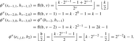
  If $k>2$, then $(s_{\nu -1,1},h_{\nu -1,1})$ is the uniquely minimized the occurrence records. If $k\le 2$, then the occurrence records of $(s_{\nu -1,1},h_{\nu -,1})$ and $(s_{\nu -2,0},h_{\nu -2,0})$ are identical and lower than the occurrence record of any other improving switch. Since the tie-breaking rule applies improving switches at selection vertices contained in higher levels first, $(s_{\nu -1,1},h_{\nu -1,1})$ is also applied first then. Consequently, $e{:}{=}(s_{\nu -1,1},h_{\nu -1,1})$ is applied next in any case.

  We prove that $\sigma$ fulfills the conditions of row 2 of Table 9. By our previous arguments, it suffices to prove that $\sigma$ has Property Usv3$_{\nu -1}$. As $\beta ^{\sigma }_{\nu }=1$, this however follows since $(s_{\nu -1,1},h_{\nu -1,1})\in I_{\sigma }$ and since $\sigma$ has Property Usv2$_{i,0}$ by the definition of a Phase-2-strategy. By our previous arguments and row 2 of Table 9, then has Properties (Usv2)$_{\nu -1,1}$, (Cc2), (Bac1)$_\nu$ and Property Usv3 for all $i<\nu -1$. Furthermore, . More precisely, if $\nu -1>2$ and $\nu >2$ implies Also note that $\nu >2$ implies by Lemma 9, so Table 2 specifies its occurrence record with respect to $\mathfrak {b}+1$.

  Consider the case $\nu -1>2$. We argue that applying improving switches according to Zadeh’s pivot rule and our tie-breaking rule then results in a sequence of strategies such that we finally obtain a strategy $\sigma '$ with $I_{\sigma '}=\mathfrak {D}^{\sigma '}\cup \{(e_{*,*,*},b_2)\}\cup \{(b_1,b_2),(s_{1,0},h_{1,0})\}$. For any $x\in \{2,\dots ,\nu -2\}$, Lemma 9 implies

  

  (1)

  Thus, $(s_{\nu -2,0},h_{\nu -2,0})$ is applied next. It is easy to verify that meets the requirements of row 2 of Table 9, so it can be used to describe the application of $(s_{\nu -2,0},h_{\nu -2,0})$.

  Let $\sigma '$ denote the strategy obtained. Then $I_{\sigma '}=\mathfrak {D}^{\sigma }\cup \{(b_{\nu -2},b_{\nu -1}),(s_{\nu -3,0},h_{\nu -3,0})\}$. Also, the occurrence record of the edge $(s_{\nu -2,0},h_{\nu -2,0})$ is described by Table 2 with respect to $\mathfrak {b}+1$. By Eq. (1) and the tie-breaking rule, $(b_{\nu -2},b_{\nu -1})$ is applied next. Similar to the previous cases, it is easy to check that row 3 of Table  9 applies to this switch. We thus obtain a strategy $\sigma$ such $\nu -2\ne 2$ implies $I_{\sigma }=\mathfrak {D}^{\sigma }\cup \{(s_{\nu -3,0},h_{\nu -3,0}),(b_{\nu -3},b_{\nu -2}),(s_{\nu -4,0},h_{\nu -4,0})\}$ and $\nu -2=2$ implies $I_{\sigma }=\mathfrak {D}^{\sigma }\cup \{(e_{*,*,*,},b_2)\}\cup \{(b_1,b_2),(s_{1,0},h_{1,0})\}.$ In either case, the occurrence record of $(b_{\nu -2},b_{\nu -1})$ is described by Table 2 with respect to $\mathfrak {b}+1$.

  In the first case, we can now apply the same arguments again iteratively as Eq. (1) remains valid for $\sigma '$ and $x\in \{2,\dots ,\nu -3\}$. After applying a finite number of improving switches we thus obtain a Phase-2-strategy $\sigma \in \varLambda _{\iota }$ with $I_{\sigma }=\mathfrak {D}^{\sigma }\cup \{(e_{*,*,*},b_2)\}\cup \{(b_1,b_2),(s_{1,0},h_{1,0})\}$. Furthermore, $\sigma$ has Property Bac1$_i$, Property Bac2$_i$ and Property Usv2$_{i,\beta ^{\sigma }_{i+1}}$ for all $i>1$ as well as Property Bac3$_i$ for all $i>1, i\ne \mu ^{\sigma }$ and Property Cc2. In addition, it holds that ${\bar{\sigma }}(g_i)=1-\beta ^{\sigma }_{i+1}$ and ${\bar{\sigma }}(d_{i,1-\beta ^{\sigma }_{i+1}})$ for all $i<\nu$ and the occurrence records of all edges applied so far (with the exception of switches $(g_*,F_{*,*})$) is described by Table 2 with respect to $\mathfrak {b}+1$. Note that this also holds if $\nu -1=2$.

  Consequently, $\sigma$ meets the requirements of row 2 of Table 9. As $\nu >2$, we have $\beta ^{\sigma }_2=0$. By Table 2, it holds that as well as 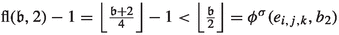. Hence, the switch $e=(s_{1,0},h_{1,0})$ is applied next and by row 2 of Table 9, is a proper Phase-3-strategy for $\mathfrak {b}$ with $I_{\sigma ^{(3)}}=\mathfrak {D}^{\sigma ^{(3)}}\cup \{(e_{i,j,k},b_2)\}\cup \{(b_1,b_2)\}$.

We thus always obtain a strategy as described by the corresponding rows of Tables 6 and 7. $\square$

We henceforth use $\sigma ^{(3)}$ to refer to the Phase-3-strategy described by Lemma 8. Note that we implicitly proved the following corollaries where the second follows by Corollary 3. Further note that we can drop the condition $\nu >1$ in Corollary 2.

Corollary 4

No cycle center is open with respect to $\sigma ^{(3)}$.

Corollary 5

Let $\sigma ^{(3)}$ be the Phase-3-strategy calculated by the Strategy Improvement resp. Policy Iteration Algorithm when starting with a canonical strategy $\sigma _{\mathfrak {b}}$ fulfilling the canonical conditions as per Lemma 8. Then, Table 2 specifies the occurrence record of every improving switch applied so far when interpreted for $\mathfrak {b}+1$, excluding switches $(g_*,F_{*,*})$, and each such switch was applied once.

1.5 Reaching either phase 4 or phase 5

We now discuss the application of improving switches during Phase 3, which highly depends on whether we have $G_n=S_n$ or $G_n=M_n$ and on the least significant set bit of $\mathfrak {b}+1$. In principle, the escape vertices are reset with respect to the new least significant bit and the targets of several cycle vertices are updated accordingly. As usual, we provide an overview describing the application of individual improving switches during Phase 3.$^{3}$ To simplify and unify the arguments, we define $t^{\rightarrow }{:}{=}\, b_2$ if $\nu >1$ and $t^{\rightarrow }{:}{=}\, g_1$ if $\nu =1$. Similarly, let $t^{\leftarrow }{:}{=}\, g_1$ if $\nu >1$ and $t^{\leftarrow }{:}{=}\, b_2$ if $\nu =1$. We furthermore define $\mathfrak {E}^{\sigma }{:}{=}\,\{(d_{i,j,k},F_{i,j}), (e_{i,j,k},t^{\rightarrow }):\sigma (e_{i,j,k})=t^{\leftarrow }\}$.

In addition, we make use of the following lemma.

Lemma 10

Let $G_n=M_n$. Let $\sigma$ be a proper Phase-3-strategy for $\mathfrak {b}$ with $\sigma \in \varLambda _{\iota }$. Let $j{:}{=}1-\beta ^{\sigma }_{i+1}$. Assume $e{:}{=}(d_{i,j,k},e_{i,j,k})\in I_{\sigma }$ and $\sigma (e_{i,j,k})=t^{\rightarrow }$ for some $k\in \{0,1\}$. Assume that there are no other indices x, y, z with $(d_{x,y,z},e_{x,y,z})\in I_{\sigma }$, that $F_{i,j}$ is closed and that $\sigma$ fulfills the following assumptions:

• 1. If $\beta ^{\sigma }_i=0$, then $\sigma (g_i)=F_{i,j}$ and $F_{i,1-j}$ is $t^{\leftarrow }$-halfopen.

• 2. $i<\mu ^{\sigma }$ implies [$\sigma (s_{i,j})=h_{i,j}$ and $\sigma (s_{i',j'})=h_{i',j'}\wedge {\bar{\sigma }}(d_{i'})$ for all $i'<i, j'\in \{0,1\}$] and that the cycle center $F_{i',1-{\bar{\sigma }}(g_{i'})}$ is $t^{\leftarrow }$-halfopen for all $i'<i$. In addition, $i<\mu ^{\sigma }-1$ implies ${\bar{\sigma }}(eb_{i+1})$.

• 3. $i'>i$ implies $\sigma (s_{i,1-\beta ^{\sigma }_{i'+1}})=b_1$.

• 4. $i'>i$ and $\beta ^{\sigma }_{i'}=0$ imply that either [${\bar{\sigma }}(g_{i'})=\beta ^{\sigma }_{i'+1}$ and $F_{i,0},F_{i,1}$ are mixed] or [${\bar{\sigma }}(g_{i'})=1-\beta ^{\sigma }_{i'+1}$, $F_{i',1-\beta ^{\sigma }_{i'+1}}$ is $t^{\rightarrow }$-open and $F_{i',\beta ^{\sigma }_{i'+1}}$ is mixed] and

• 5. $i'>i$ and $\beta ^{\sigma }_{i'}=1$ imply that $F_{i',1-\beta ^{\sigma }_{i'+1}}$ is either mixed or $t^{\rightarrow }$-open.

Then is a proper Phase-3-strategy for $\mathfrak {b}$ with and if $i<\mu ^{\sigma }$ and otherwise.

Table 10 Improving switches applied during Phase 3

The next lemma descries the application of switches of the type $(d_{i,j,k},e_{i,j,k})$ for several cases.

Lemma 11

Let $\sigma \in \varLambda _{\sigma ^{(3)}}$ be a proper Phase-3-strategy for $\mathfrak {b}$ obtained through the application of a sequence $\mathfrak {A}_{\sigma ^{(3)}}^{\sigma }\subseteq \mathbb {E}^1\cup \mathbb {D}^0$ of improving switches. Assume that the conditions of row 1 of Table 10 are fulfilled for each intermediate strategy $\sigma '$. Let $e=(d_{i,j,k}, e_{i,j,k})\in I_{\sigma }$ be the switch applied next and assume $\sigma (e_{i,j,k})=t^{\rightarrow }, \beta ^{\sigma }_{i}=0\vee \beta ^{\sigma }_{i+1}\ne j$ and $I_{\sigma }\cap \mathbb {D}^0=\{e\}$. Further assume that either $i\ge \nu$ or that $G_n=S_n$. Then is a proper Phase-3-strategy for $\mathfrak {b}$ with .

The next lemma now summarizes the application of improving switches during Phase 3. Depending on whether we consider PG or $M_n$ and depending on $\nu$, we then either obtain a Phase-4-strategy or a Phase-5-strategy for $\mathfrak {b}$.

Lemma 9

Let $\sigma _{\mathfrak {b}}\in \varLambda _{\iota }$ be a canonical strategy for $\mathfrak {b}\in \mathcal {B}_n$ fulfilling the canonical conditions. After applying a finite number of improving switches, the Strategy Improvement resp. Policy Iteration Algorithm produces a strategy $\sigma$ with the following properties: If $\nu >1$, then $\sigma$ is a Phase-k-strategy for $\mathfrak {b}$, where $k=4$ if $G_n=S_n$ and $k=5$ if $G_n=M_n$. If $\nu =1$, then $\sigma$ is a Phase-5-strategy for $\mathfrak {b}$. In any case, $\sigma \in \varLambda _{\iota }$ and $\sigma$ is described by the corresponding rows of Tables 6 and 7.

Proof

By Lemma 8, applying improving switches according to Zadeh’s pivot rule and our tie-breaking rule yields a proper Phase-3-strategy $\sigma ^{(3)}\in \varLambda _{\iota }$ described by the corresponding row of Table 6 and 7. We begin by describing Phase 3 informally.

For every cycle vertex, either $\sigma ^{(3)}(d_{i,j,k})=F_{i,j}$ or $\sigma ^{(3)}(d_{i,j,k})=e_{i,j,k}$ and $(d_{i,j,k},F_{i,j})\in I_{\sigma ^{(3)}}$. It will turn out that only switches corresponding to cycle vertices of the first type are applied during Phase 3. For each such cycle vertex $d_{i,j,k}$, the switch $(e_{i,j,k},t^{\rightarrow })$ will be applied. If $(\mathfrak {b}+1)_i=0$ or $(\mathfrak {b}+1)_{i+1}\ne j$, then $(d_{i,j,k},e_{i,j,k})$ becomes improving and is applied next. This then goes on until all such improving switches have been applied. During this procedure, it might happen that an edge $(s_{i',*},b_1)$ with $i'<\nu$ becomes improving after applying some switch $(d_{i,j,k},e_{i,j,k})$ if we consider $G_n=M_n$ and if we have $\nu >1$. In this case, the corresponding switch is applied immediately. Finally, $(b_1,b_2)$ resp. $(b_1,g_1)$ is applied, resulting in a Phase-4-strategy in $S_n$ if $\nu >1$ and in a Phase-5-strategy otherwise.

We now formalize this behavior. Using Lemma 8 and Table 2, it is easy to verify that switches $(e_{*,*,*},t^{\rightarrow })$ minimize the occurrence record among all improving switches.$^{3}$. By the tie-breaking rule, a switch $(e_{i,j,k},t^{\rightarrow })$ with $\sigma ^{(3)}(d_{i,j,k})=F_{i,j}$ is thus applied next. Since $\sigma ^{(3)}(s_{i',*})=h_{i',*}$ for all $i'<\mu ^{\sigma ^{(3)}}$ by Lemma 8, the statement of row 1 of Table 10 can be applied.

In addition, it is easy to verify that the characterization given in this row implies that we have if $\beta ^{\sigma }_{i}=0\vee \beta ^{\sigma }_{i+1}\ne j$ and else.$^{3}$ Consequently, by the tie-breaking rule and row 1 of Table 10, improving switches $(e_{*,*,*},t^{\rightarrow })\in \mathbb {E}^1$ are applied until a switch with $\beta ^{\sigma }_i=0\vee \beta ^{\sigma }_{i+1}\ne j$ is applied. Note that the occurrence record of each applied switch is described by Table 2 when interpreted for $\mathfrak {b}+1$ since $\left\lfloor \frac{\mathfrak {b}}{2}\right\rfloor +1=\mathfrak {m}$ if $\mathfrak {b}$ is odd and $\left\lceil \frac{\mathfrak {b}}{2}\right\rceil +1=\left\lceil \frac{\mathfrak {b}+1}{2}\right\rceil$ if $\mathfrak {b}$ is even. By row 1 of Table 10, $(d_{i,j,k},e_{i,j,k})$ then becomes improving. As $(d_{i,j,k},e_{i,j,k})\notin \mathfrak {A}_{\sigma _{\mathfrak {b}}}^{\sigma }$ and since switches of the type $(e_{*,*,*},t^{\rightarrow })$ minimize the occurrence record, Table 2 and the tie-breaking rule imply that $(d_{i,j,k},e_{i,j,k})$ is applied next. In particular, an edge $(d_{i,j,k},e_{i,j,k})$ is applied immediately if it becomes improving and this requires that $(e_{i,j,k},t^{\rightarrow })$ was applied earlier. Thus, their occurrence record is described by Table 2 when interpreted for $\mathfrak {b}+1$. Therefore, the application of improving switches $(e_{*,*,*},t^{\rightarrow })$ is described by row 1 of Table 10 and whenever an edge $(d_{*,*,*},e_{*,*,*})$ becomes improving, its application is described by Lemma 11.

Let $G_n=S_n$. Then, row 1 of Table 10 and Lemma 11 can be applied until a strategy $\sigma$ is reached such that all improving switches $(e_{i,j,k},t^{\rightarrow })$ with $\sigma ^{(3)}(d_{i,j,k})=F_{i,j}$ were applied. As $(d_{i,j,k},e_{i,j,k})$ was applied if and only if $\beta ^{\sigma }_i=0\vee \beta ^{\sigma }_{i+1}=j$, this implies that $\sigma (d_{i,j,k})=F_{i,j}$ is equivalent to $\beta ^{\sigma }_i=1\wedge \beta ^{\sigma }_{i+1}=j)$. Consequently, every cycle center is closed or escapes towards $t^{\rightarrow }$. In addition, an edge $(d_{i,j,k},F_{i,j})$ is an improving switch exactly if the switch $(e_{i,j,k},t^{\rightarrow })$ was not applied. Consequently, $I_{\sigma }=\{(d_{i,j,k},F_{i,j}), (e_{i,j,k}, t^{\rightarrow }):\sigma (e_{i,j,k})=t^{\leftarrow }\}\cup \{(b_1,t^{\rightarrow })\}.$ Now, as $\phi ^{\sigma }(b_1,t^{\rightarrow })=\phi ^{\sigma }(e_{*,*,*},t^{\rightarrow })$ and $\mathbb {E}^1=\emptyset$, the switch $e{:}{=}(b_1,t^{\rightarrow })$ is applied next due to the tie-breaking rule. We prove that we can apply row 2 resp. 4 of Table 10, implying the statement follows for $G_n=S_n$ with arbitrary $\nu$ and for $G_n=M_n$ with $\nu =1$.

We thus prove the following. If $\nu >1$, then ${\bar{\sigma }}(eb_{i,j})\wedge \lnot {\bar{\sigma }}(eg_{i,j})$ for all $(i,j)\in S_1$ and, in addition, ${\bar{\sigma }}(eb_{i,j})\wedge {\bar{\sigma }}(eg_{i,j})$ for all $(i,j)\in S_2$. If $\nu =1$, then ${\bar{\sigma }}(eg_{i,j})\wedge \lnot {\bar{\sigma }}(eb_{i,j})$ for all $(i,j)\in S_4$ and ${\bar{\sigma }}(eb_{i,j})\wedge {\bar{\sigma }}(eg_{i,j})$ for all $(i,j)\in S_3$. We begin by observing that the definition of the sets $S_1$ to $S_4$ implies that $\beta ^{\sigma }_i=0\vee \beta ^{\sigma }_{i+1}\ne j$ for all of the relevant indices. Also, $(e_{i,j,k},t^{\rightarrow })\in \mathfrak {A}_{\sigma ^{(3)}}^{\sigma }$ if and only if $\sigma ^{(3)}(d_{i,j,k})=F_{i,j}$. Thus, $(e_{i,j,k},t^{\rightarrow })\notin \mathfrak {A}_{\sigma ^{(3)}}^{\sigma }$ if and only if $\sigma ^{(3)}(d_{i,j,k})=e_{i,j,k}$. Since $e_{i,j,k}$ has an outdegree of 2, this implies $(\sigma (e_{i,j,k})=t^{\leftarrow }\Leftrightarrow \sigma ^{(3)}(d_{i,j,k})=e_{i,j,k})$. In particular, due to $\beta ^{\sigma }_i=0\vee \beta ^{\sigma }_{i+1}\ne j$, the switch $(d_{i,j,k}, e_{i,j,k})$ was then also applied. Hence, if there is a $k\in \{0,1\}$ with $\sigma ^{(3)}(d_{i,j,k})=e_{i,j,k}$, then ${\bar{\sigma }}(eg_{i,j})$ if $\nu >1$ resp. ${\bar{\sigma }}(eb_{i,j})$ if $\nu =1$.

Since every cycle center is closed or escapes to $t^{\rightarrow }$ with respect to $\sigma$, either ${\bar{\sigma }}(eb_{i,j})\wedge {\bar{\sigma }}(eg_{i,j})$ or ${\bar{\sigma }}(eb_{i,j})\wedge \lnot {\bar{\sigma }}(eg_{i,j})$ or ${\bar{\sigma }}(d_{i,j})$ for all cycle centers $F_{i,j}$ if $\nu >1$. Similarly, for $\nu =1$, either ${\bar{\sigma }}(eb_{i,j})\wedge {\bar{\sigma }}(eg_{i,j})$ or ${\bar{\sigma }}(eg_{i,j})\wedge \lnot {\bar{\sigma }}(eb_{i,j})$ or ${\bar{\sigma }}(d_{i,j})$ for all cycle centers $F_{i,j}$. Consequently, the cycle centers $F_{i,j}$ with ${\bar{\sigma }}(eb_{i,j})\wedge {\bar{\sigma }}(eg_{i,j})$ are exactly the cycle centers that contain a vertex $d_{i,j,k}$ with $\sigma _{\mathfrak {b}}(d_{i,j,k})\ne F_{i,j}$ and such that $(d_{i,j,k},F_{i,j})$ was not applied during Phase 1. By Lemma 8, all improving switches $(d_{i,j,k},F_{i,j})$ not applied in Phase 1 had $\phi ^{\sigma _{\mathfrak {b}}}(d_{i,j,k},F_{i,j})=\mathfrak {m}$. By Corollary 4, it thus suffices to prove that there is a $k\in \{0,1\}$ with $\phi ^{\sigma _{\mathfrak {b}}}(d_{i,j,k},F_{i,j})=\mathfrak {m}$ to prove ${\bar{\sigma }}(eb_{i,j})\wedge {\bar{\sigma }}(eg_{i,j})$. Analogously, to prove ${\bar{\sigma }}(eb_{i,j})\wedge \lnot {\bar{\sigma }}(eg_{i,j})$ resp. ${\bar{\sigma }}(eg_{i,j})\wedge \lnot {\bar{\sigma }}(eb_{i,j})$, it suffices to show that $F_{i,j}$ was closed at the end of Phase 1.

We now prove the corresponding statements for the case $\nu >1$ and omit the case $\nu =1$.$^{3}$ Let $m=\max \{i:\sigma (b_i)=g_i\}$ and $u=\min \{i:\sigma (b_i)=b_{i+1}\}$.

• 1. We prove that $\phi ^{\sigma _{\mathfrak {b}}}(d_{i,j,0},F_{i,j})=\mathfrak {m}$ for all $(i,j)\in S_2$.

  • Let $i\le \nu -1$ and $j=\beta ^{\sigma }_{i+1}$. Then, $\mathfrak {b}_{i+1}\ne (\mathfrak {b}+1)_{i+1}=\beta ^{\sigma }_{i+1}$ as $i\le \nu -1$, so $j\ne \mathfrak {b}_{i+1}$. Thus, there is a feasible $t_{\mathfrak {b}}$ for $\mathfrak {b}$ with $\phi ^{\sigma _{\mathfrak {b}}}(d_{i,j,k},F_{i,j})=\min \left( \left\lfloor \frac{\mathfrak {b}+1-k}{2}\right\rfloor ,\ell ^{\mathfrak {b}}(i,j,k)+t_{\mathfrak {b}}\right) .$ However, since $i\le \nu -1$, $\mathfrak {b}_i=1$ and thus $t_{\mathfrak {b}}=0$ is the only feasible parameter. It thus suffices to show $\ell ^{\mathfrak {b}}(i,j,0)\ge \mathfrak {m}$. Since $\mathfrak {b}_i=1\wedge j\ne \mathfrak {b}_{i+1}$, this follows from Lemma 7.

  • Let $i\in \{\nu +1,\dots ,m\},\beta ^{\sigma }_i=1$ and $j=1-\beta ^{\sigma }_{i+1}$. Since $i>\nu$ implies $\beta ^{\sigma }_{i}=\mathfrak {b}_i$ and $\beta ^{\sigma }_{i+1}=\mathfrak {b}_{i+1}$, $\ell ^{\mathfrak {b}}(i,j,0)\ge \mathfrak {m}$ follows as in the previous case.

  • Let $i\in \{\nu ,\dots ,m-1\}\wedge \beta ^{\sigma }_i=0$ and $j=\beta ^{\sigma }_{i+1}$. Since $i+1>\nu$ implies that we have $\beta ^{\sigma }_{i+1}=\mathfrak {b}_{i+1}, \mathfrak {b}_{\nu -1}=1$ and $\nu \ge 2$, we obtain $\ell ^{\mathfrak {b}}(i,j,0)>\mathfrak {m}+1$ by an easy calculation. Thus, $\ell ^{\mathfrak {b}}(i,j,k)+t_{\mathfrak {b}}>\mathfrak {m}$ for every $t_{\mathfrak {b}}$ feasible for $\mathfrak {b}$, implying $\phi ^{\sigma _{\mathfrak {b}}}(d_{i,j,0},F_{i,j})=\mathfrak {m}$.

  • Let $i>m$ and $j\in \{0,1\}$. Then, since $\mathfrak {b}'_i=0$ for all $\mathfrak {b}'\le \mathfrak {b}$. Hence, by Lemma 7, $\ell ^{\mathfrak {b}}(i,j,k)\ge \mathfrak {b}$. Consequently, $\phi ^{\sigma _{\mathfrak {b}}}(d_{i,j,0},F_{i,j})=\mathfrak {m}.$

  • Assume $\mathfrak {b}+1=2^{l}$ for some $l\in \mathbb {N}$. Then $\nu =l+1$ and $\mathfrak {b}_{\nu }=0$. This implies , hence $\phi ^{\sigma _{\mathfrak {b}}}(d_{i,j,0},F_{i,j})=\mathfrak {m}$.

• 2. We prove that either ${\overline{\sigma }_{\mathfrak {b}}}(d_{i,j})$ or $\phi ^{\sigma _{\mathfrak {b}}}(d_{i,j,k},F_{i,j})<\mathfrak {m}$ for both $k\in \{0,1\}$ for all $(i,j)\in S_1$.

  • Let $i\le \nu -1$ and $j=1-\beta ^{\sigma }_{i+1}$. Then $\mathfrak {b}_i=1$ and $j=1-\beta ^{\sigma }_{i+1}=\mathfrak {b}_{i+1}$. Hence $F_{i,j}$ was closed with respect to $\sigma _{\mathfrak {b}}$.

  • Let $i\in \{\nu ,\dots ,m-1\}, \beta ^{\sigma }_{i}=0$ and $j=1-\beta ^{\sigma }_{i+1}$. Then $\mathfrak {b}_i=\beta ^{\sigma }_{i}=0, \beta ^{\sigma }_{i+1}=\mathfrak {b}_{i+1}$ and $\beta ^{\sigma }_i=0$ implies $i\ne \nu$. In particular, $\nu \le i-1$ and $\mathfrak {b}_\nu =0$. Using Lemma 7, this implies $\ell ^{\mathfrak {b}}(i,j,k)\le \left\lfloor \frac{\mathfrak {b}+1-k}{2}\right\rfloor -1$. This implies $\ell ^{\mathfrak {b}}(i,j,k)+1\le \lfloor \frac{\mathfrak {b}+1-k}{2}\rfloor$, hence $\phi ^{\sigma _{\mathfrak {b}}}(d_{i,j,k},F_{i,j})\le \ell ^{\mathfrak {b}}(i,j,1)+1$. If this inequality is strict, the statement follows. If the inequality is tight, then $\sigma _{\mathfrak {b}}(d_{i,j,k})=F_{i,j}$ by Property Or2$_{i,j,k}$ and Property Or1$_{i,j,k}$ thus implies $\phi ^{\sigma _{\mathfrak {b}}}(d_{i,j,k},F_{i,j})<\mathfrak {m}$.

  • Assume that there is no $l\in \mathbb {N}$ with $\mathfrak {b}+1=2^l$ and let $i=\nu$ and $j=1-\mathfrak {b}_{\nu +1}$. Since $\mathfrak {b}$ is odd, Property Or3$_{i,j,0}$ implies $\phi ^{\sigma _{\mathfrak {b}}}(d_{i,j,0},F_{i,j})<\mathfrak {m}.$ For $k=1$, $\mathfrak {b}$ being odd implies $\phi ^{\sigma _{\mathfrak {b}}}(d_{i,j,1},F_{i,j})\le \left\lfloor \frac{\mathfrak {b}+1-1}{2}\right\rfloor =\left\lfloor \frac{\mathfrak {b}}{2}\right\rfloor <\mathfrak {m}$.

By row 2 of Table 10, the statement follows for $G_n=S_n$ if $\nu >1$. In addition, by row 4 of Table 10, the statement follows for $\nu =1$.

It remains to consider the case $\nu >1$ if $G_n=M_n$, implying $t^{\rightarrow }=b_2$ and $t^{\leftarrow }=g_1$. Using the same argumentation as before, row 1 of Table 10 and Lemma 11 imply that improving switches within levels $i\ge \nu$ are applied until we obtain a proper Phase-3-strategy $\sigma$ for $\mathfrak {b}$ with

$$\begin{aligned} I_{\sigma }&=\{(d_{i,j,k},F_{i,j}):i<\nu \wedge \sigma (d_{i,j,k})\ne F_{i,j}\}\\&\cup \{(d_{i,j,k},F_{i,j}),(e_{i,j,k},b_2):i\ge \nu \wedge \sigma (e_{i,j,k})=g_1\}\cup \{(b_1,b_2)\}. \end{aligned}$$

As no cycle center in any level $i'<\nu$ was opened yet, the switch $e=(e_{i,j,k},b_2)$ with $i=\nu -1, j=1-\beta ^{\sigma }_{i+1}$ and $k\in \{0,1\}$ is applied next. Since $\sigma (d_{i,j,k})=F_{i,j}$, row 1 of Table 10 implies . Due to the tie-breaking rule, $(d_{i,j,k},e_{i,j,k})$ is applied next. We prove that $\sigma$ meets the requirements of Lemma 10.

There are no other indices $i',j',k'$ with . Also, as no such switch was applied yet in any level below level i, $F_{i,j}$ is closed for as it was closed for $\sigma ^{(3)}$ by Lemma 8. As $i<\nu$ and , Definition 4 implies $\sigma _{\mathfrak {b}}(g_i)=F_{i,j}$. By the same arguments used when discussing the case $G_n=S_n$, it can be proven that $F_{i,1-j}$ was not closed during Phase 1 as $(i,1-j)\in S_2$. Consequently, follows from Corollary 2. By the tie-breaking rule, no improving switch involving $F_{i,1-j}$ was applied yet. Therefore, as well as . By Corollary 4, $F_{i,1-j}$ cannot be open for $\sigma ^{(3)}$, so it is not open for . Therefore, as and , it is $g_1$-halfopen. Thus, the first requirement of Lemma 10 is met.

By Lemma 8 and since for any $i'<\nu$, for all $i'<\nu$. Furthermore, $i'<\nu$ implies $\mathfrak {b}_{i'}=1$ and no improving switch $(d_{*,*,*},e_{*,*,*})$ below level $\nu$ was applied yet. Consequently, for all $i'<\nu$. Now consider some cycle center $F_{i',j'}$ where $i'<i$ and . We prove that $F_{i',j'}$ is $g_1$-halfopen. The cycle center is not closed while is closed due to . Thus, by Corollary 2 and the same arguments used before, and, in particular, . However, by Corollary 4 and the tie-breaking rule, this implies that $F_{i',j'}$ is $g_1$-halfopen as before. Thus, the second requirement of Lemma 10 is met.

The third requirement is met as $i'>i=\nu -1$ and since has Property Usv1$_{i'}$.

Consider the fourth requirement. Let $i'>i$ and $\beta ^{\sigma }_{i'}=0$. Then, due to the tie-breaking rule, all improving switches $(e_{i',j',k'},b_2)$ with $\sigma ^{(3)}(d_{i',j',k'})=F_{i',j'}$ have already been applied. Since $\beta ^{\sigma }_{i'}=0$, $F_{i',\beta ^{\sigma }_{i'+1}}$ cannot have been closed for $\sigma ^{(3)}$. If both cycle centers of level $i'$ were $g_1$-halfopen for $\sigma ^{(3)}$, then they are mixed for $\sigma$, and $\sigma (g_{i'})=\sigma ^{(3)}(g_{i'})=\sigma _{\mathfrak {b}}(g_{i'})=F_{i',\beta ^{\sigma }_{i'+1}}$. If $F_{i',1-\beta ^{\sigma }_{i'+1}}$ is closed for $\sigma ^{(3)}$, then $F_{i',\beta ^{\sigma }_{i'+1}}$ can only be $g_1$-halfopen for $\sigma ^{(3)}$. Consequently, by Corollary 2 resp. Definition 4, ${\bar{\sigma }}(g_{i'})=1-\beta ^{\sigma }_{i'+1}$. Furthermore, $F_{i',1-\beta ^{\sigma }_{i'+1}}$ is then $b_2$-open and $F_{i',\beta ^{\sigma }_{i'+1}}$ is $b_2$-halfopen (for $\sigma$). Thus, the fourth requirement is met.

By the same argument, if $i'>i$ and $\beta ^{\sigma }_{i'+1}=1$, then $\smash {F_{i',1-\beta ^{\sigma }_{i'+1}}}$ is $b_2$-open if it was closed for $\sigma ^{(3)}$ and mixed if it was $g_1$-halfopen. Thus, the fifth and final requirement is met.

Therefore, the application of $(d_{i,j,k},e_{i,j,k})$, yields a proper Phase-3-strategy $\sigma \in \varLambda _{\iota }$ for $\mathfrak {b}$ with . We prove $\phi ^{\sigma }(s_{i,j},b_1)<\phi ^{\sigma }(e_{i,j,k},b_2)=\left\lfloor \frac{\mathfrak {b}}{2}\right\rfloor$, implying that $(s_{i,j},b_1)$ is applied next. It is easy to verify that $(s_{i,j},b_1)\notin \mathfrak {A}_{\sigma _{\mathfrak {b}}}^{\sigma }$. Consequently, by Table 2 and as $i=\nu -1$ and $j=1-\beta ^{\sigma }_{i+1}=0$, if $\mathfrak {b}\ge 3$ since $\nu \ge 2$. If $\mathfrak {b}_1=1$, then$(s_{i,j},b_1)$ is also the next switch applied as the tie-breaking rule then ranks $(s_{i,j},b_1)$ higher than any switch $(e_{*,*,*},b_2)$. Since $(e_{i,j,k},b_2), (d_{i,j,k},e_{i,j,k})\in \mathfrak {A}_{\sigma _{\mathfrak {b}}}^{\sigma }$ and since $F_{i,j}$ was closed $(e_{i,j,k},b_2)$ was applied, we have ${\bar{\sigma }}(eb_{i,j})\wedge \lnot {\bar{\sigma }}(eg_{i,j})$. Therefore, the last row of Table 10 describes the application of $e=(s_{i,j},b_1)$. Consequently, is a proper Phase-3-strategy with and by Lemma 9. Thus, Table 2 describes the occurrence record of $(s_{i,j},b_1)$ when interpreted for $\mathfrak {b}+1$. Since $F_{i,j}$ is $b_2$-halfopen for whereas $F_{i,1-j}$ is $g_1$-halfopen, $(e_{i,j,1-k},b_2)$ is applied next. By the first row of Table 10, this application unlocks $(d_{i,j,1-k},e_{i,j,1-k})$. Using our previous arguments and observations, it is easy to verify that $(d_{i,j,1-k},e_{i,j,1-k})$ is applied next and that its application is described by the second-to-last row of Table 10. The tie-breaking rule then chooses to apply $(e_{i,1-j,k},b_2)\in \mathbb {E}^1$ next. By row 1 of Table 10, $(d_{i,1-j,k},e_{i,1-j,k})$ then becomes improving and is applied next. Its application is described by row 5 of Table 10. After applying this switch, we then obtain a strategy $\sigma$ with

It is easy to verify that the same arguments can be applied iteratively as applying a switch $(s_{i',j'},b_1)$ with $i'<\nu$ always requires to open the corresponding cycle center $F_{i',j'}$ first. Thus, after finitely many iterations, we obtain a strategy $\sigma$ with $I_{\sigma }=\{(d_{i,j,k},F_{i,j}), (e_{i,j,k}, b_2):\sigma (e_{i,j,k})=g_1\}\cup \{(b_1,b_2)\}.$ By the same arguments used for the case $G_n=S_n$, the conditions of the third row of Table 10 are met, so we obtain a strategy as described by the corresponding rows of Tables 6 and 7. $\square$

We henceforth use $\sigma ^{(3)}$ to refer to the Phase-3-strategy described by Lemma 8. As before, we implicitly proved the following corollary which follows from Corollary 5.

Corollary 6

Let $\sigma ^{(4)}$ be the Phase-4-strategy calculated by the Strategy Improvement resp. Policy Iteration Algorithm when starting with a canonical strategy $\sigma _{\mathfrak {b}}$ fulfilling the canonical conditions as per Lemma 9. Then, Table 2 specifies the occurrence record of every improving switch applied so far when interpreted for $\mathfrak {b}+1$, excluding switches $(g_*,F_{*,*})$, and each such switch was applied once.

1.6 Reaching phase 5 if there is a phase 4

As shown by Lemma 9, we do not always obtain a Phase-5-strategy immediately after Phase 3 as we have to apply improving switches involving selection vertices $s_{i,*}$ in levels $i<\nu$ if $G_n=S_n$. We thus prove that we also reach a Phase 5 strategy after applying these switches. Consequently, we always reach a Phase 5 strategy. The application of all of these switches is captured by the following lemma.

Lemma 12

Let $G_n=S_n$. Let $\sigma \in \varLambda _{\iota }$ be a Phase-4-strategy for $\mathfrak {b}\in \mathcal {B}_n$ with $\nu >1$. Assume $e{:}{=}\, (s_{i,1-\beta ^{\sigma }_{i+1}},b_1)\in I_{\sigma }$ for some $i<\nu$. Further assume that $\sigma$ has Property Usv1$_{i'}$ for all $i'>i$ and that $\sigma (d_{i',j',k'})=F_{i',j'}\Leftrightarrow \beta ^{\sigma }_{i'}=1\wedge \beta ^{\sigma }_{i'+1}=j'$. Moreover, assume that $i'<\nu$ implies ${\bar{\sigma }}(g_{i'})=1-\beta ^{\sigma }_{i'+1}$ and that $i'<i$ implies $\sigma (s_{i',*})=h_{i',*}$. If $(s_{i',1-\beta ^{\sigma }_{i'+1}},b_1)\in I_{\sigma }$ for some $i'<i$, then is a Phase-4-strategy for $\mathfrak {b}$. Otherwise, it is a Phase-5-strategy for $\mathfrak {b}$. In either case, .

We now state the lemma describing the application of the improving switches during Phase 4.

Lemma 10

Let $\sigma _{\mathfrak {b}}\in \varLambda _{\iota }$ be a canonical strategy for $\mathfrak {b}\in \mathcal {B}_n$ fulfilling the canonical conditions. After applying a finite number of improving switches, the Strategy Improvement resp. Policy Iteration Algorithm produces a Phase-5-strategy $\sigma ^{(5)}\in \varLambda _{\iota }$ as described by the corresponding rows of Tables 6 and 7.

Proof

By Lemma 9, it suffices to consider the case $G_n=S_n$ and $\nu >1$. By Lemma 9, the Strategy Improvement Algorithm calculates a Phase-4-strategy $\sigma$ for $\mathfrak {b}$ with $\sigma \in \varLambda _{\iota }$ and

We show that $(s_{\nu -1,0},b_1)$ is applied next. Assume that $\mathfrak {b}+1$ is a power of two, implying $\mathfrak {b}=2^{\nu -1}-1$. It is easy to verify that $(s_{\nu -1,0},b_1)$ and $(s_{\nu -2,1},b_1)$ both minimize the occurrence record if $\mathfrak {b}>1$.$^{3}$ If $\mathfrak {b}=1$, then the switches $(e_{i,j,k},b_2)$ with $\sigma (e_{i,j,k})=g_1$ also minimize the occurrence record. Due to the tie-breaking rule, $(s_{\nu -1,0},b_1)$ is however applied next in any case.

If $\mathfrak {b}+1$ is not a power of two, then $\mathfrak {b}\ge 2^{\nu }+2^{\nu -1}-1$ and $\mathfrak {b}\ge 6$, implying $\left\lfloor \frac{\mathfrak {b}+2}{4}\right\rfloor <\mathfrak {m}$ as well as $\left\lfloor \frac{\mathfrak {b}+2}{4}\right\rfloor <\left\lfloor \frac{\mathfrak {b}}{2}\right\rfloor$. It is again easy to verify that this implies that $(s_{\nu -1,0},b_1)$ minimizes the occurrence record.$^{3}$ Thus, the switch $e=(s_{\nu -1,0},b_1)$ is applied next in any case. We now prove that Lemma 12 describes the application of e. Since $\sigma$ is a Phase-4-strategy and since $i'>i=\nu -1$ implies $i'\ge \nu$, $\sigma$ has Property Usv1$_{i'}$ for all $i'>i$. By Lemma 9, it follows that $\sigma$ also meets the other requirements of Lemma 12.

Consider the case $\nu =2$ first. Then, applying $e=(s_{1,0},b_1)$ yields a Phase-5-strategy and by Lemma 9. Hence, Table 2 describes the occurrence record of e with respect to $\mathfrak {b}+1$. In addition, we then have

Since is a Phase-5-strategy, it has Property Rel1, implying . Thus, has all properties listed in the corresponding rows of Tables 6 and 7.

Before discussing the case $\nu >2$, we discuss edges $(d_{i,j,k},F_{i,j})$ that become improving when a switch $(s_{i,j},b_1)$ with $i<\nu$ and $j=1-\beta ^{\sigma }_{i+1}$ is applied, see Lemma 12. Since $i<\nu$ implies $1-\beta ^{\sigma }_{i+1}=\mathfrak {b}_{i+1}$, their cycle centers $F_{i,j}$ were closed for $\sigma _{\mathfrak {b}}$. Therefore, their occurrence record might be very low. However, their occurrence records are not “too low” in the sense that they interfere with the improving switches applied during Phase 4. More precisely, it can be shown that $i<\nu$ and $j=\mathfrak {b}_{i+1}$ imply $\phi ^{\sigma _{\mathfrak {b}}}(d_{i,j,k},F_{i,j})>\left\lfloor \frac{\mathfrak {b}+2}{4}\right\rfloor -1$.$^{3}$

We now consider case $\nu >2$. We obtain as before. Furthermore,

by Lemma 12. We show that the switches $(s_{\nu -2,1},b_1),\dots ,(s_{1,1},b_1)$ are applied next and in this order. To simplify notation, we denote the current strategy by $\sigma$. By Table 2, it holds that for all $i\le \nu -2$. Hence $\phi ^{\sigma }(s_{\nu -2,1},b_1)<\dots <\phi ^{\sigma }(s_{1,1},b_1)$ by Lemma 9. It thus suffices to show that the occurrence record of $\phi ^{\sigma }(s_{1,1},b_1)$ is smaller than the occurrence record of any switch improving for $\sigma$ and any improving switch that might be unlocked by applying some switch $(s_{i,1},b_1)$ for $i\le \nu -2$.

The second statement follows since and since the occurrence record of any edge that becomes improving is bounded by $\left\lfloor \frac{\mathfrak {b}+2}{4}\right\rfloor$ as discussed earlier. It thus suffices to show the first statement. Let $e{:}{=}(d_{i,j,k},F_{i,j})\in I_{\sigma }$ such that $\sigma (e_{i,j,k})=g_1$. By Lemma 8 and Lemma 9, this implies . Then, $\nu >2$ implies , hence $\phi ^{\sigma }(e)<\phi ^{\sigma }(s_{1,1},b_1)$. Next let $e{:}{=}(e_{i,j,k},b_2)\in I_{\sigma }$ such that $\sigma (e_{i,j,k})=g_1$. Then, since $\mathfrak {b}$ is odd, Table 2 implies , hence $\phi ^{\sigma }(e)>\phi ^{\sigma }(s_{1,1},b_1)$. If $\mathfrak {b}+1$ is not a power of two, we need to show this estimation for some more improving switches. But this can be shown by the easy calculations similar to the calculations necessary when discussing the application of $(s_{\nu -1,0},b_1)$.

Consequently, the switches $(s_{\nu -1},b_1),\dots ,(s_{1,1},b_1)$ are applied next by the Strategy Improvement Algorithm and in this order. It is easy to verify that the requirements of Lemma 12 are always met, so this lemma describes the application of these switches. It is also easy to check that the occurrence record of these edges is described by Table 2 after applying them. Let $\sigma$ denote the strategy obtained after applying $(s_{1,1},b_1)$. Then $\sigma$ is a Phase-5-strategy for $\mathfrak {b}$ with $\sigma \in \varLambda _{\iota }$ and $\mu ^{\sigma }=\min \{i:\beta ^{\sigma }_i=0\}$. This further implies

$$\begin{aligned} I_{\sigma }=&\,\{(d_{i,j,k},F_{i,j}),(e_{i,j,k},b_2):\sigma (e_{i,j,k})=g_1\}\\ \cup&\,\{(d_{i,1-(\mathfrak {b}+1)_{i+1},*},F_{i,1-(\mathfrak {b}+1)_{i+1}}):i\le \nu -1\}\cup X_0\cup X_1 \end{aligned}$$

Further note that $\sigma (e_{i,j,k})=g_1$ still implies $\phi ^{\sigma _{\mathfrak {b}}}(d_{i,j,k},F_{i,j})=\phi ^{\sigma }(d_{i,j,k},F_{i,j})=\mathfrak {m}$ since the corresponding switches are improving since the end of Phase 1. Also, every improving switch was applied at most once and we proved that the occurrence record of any improving switch that was applied is described correctly by Table 2 when interpreted for $\mathfrak {b}+1$. Since no improving switch involving cycle vertices were applied, we also still have $\sigma ^{\omega }(d_{i,j,k})=F_{i,j}$ if and only of $(\mathfrak {b}+1)_i=1$ and $(\mathfrak {b}+1)_{i+1}=j$. Hence, all conditions listed in the corresponding rows of Tables 6 and 7 are fulfilled, proving the statement. $\square$

We henceforth use $\sigma ^{(3)}$ to refer to the Phase-3-strategy described by Lemma 8. As before, we implicitly proved the following corollary which follows from Corollaries 5 and 6.

Corollary 7

Let $\sigma ^{(5)}$ be the Phase-5-strategy calculated by the Strategy Improvement resp. Policy Iteration Algorithm when starting with a canonical strategy $\sigma _{\mathfrak {b}}$ fulfilling the canonical conditions as per Lemma 10. Then, Table 2 specifies the occurrence record of every improving switch applied so far when interpreted for $\mathfrak {b}+1$, excluding switches $(g_*,F_{*,*})$, and each such switch was applied once.

1.7 Reaching a canonical strategy for $\mathfrak {b}+1$

We now prove Lemma 5. It states that applying improving switches according to Zadeh’s pivot rule and our tie-breaking rule produces the strategies described by Tables 7 and 6. In particular, it states that we obtain a canonical strategy for $\mathfrak {b}+1$ fulfilling the canonical conditions. We split the proof as follows. First, we observe that it only remains to prove Lemma 5 for $k=5$. We then prove that we obtain a canonical strategy for $\mathfrak {b}+1$ and show that this strategy fulfills the canonical conditions afterwards. These two statements thus imply Lemma 5 for $k=5$.

We first provide an overview describing the application of improving switches during Phase 5.$^{3}$

Table 11 Improving switches applied during Phase 5

The following lemma describes the application if switches $(e_{i,j,k},t^{\rightarrow })$ during Phase 5. As it is rather involved, we state it separately and do not include it into Table 11.

Lemma 13

Let $\sigma \in \varLambda _{\iota }$ be a Phase-5-strategy for $\mathfrak {b}\in \mathcal {B}_n$. Let $e{:}{=}(e_{i,j,k},t^{\rightarrow })\in I_{\sigma }$ and let $F_{i,j}$ be mixed. Assume that $\nu >1\Rightarrow \lnot {\bar{\sigma }}(eg_{i,1-j})$ and $\nu =1\Rightarrow \lnot {\bar{\sigma }}(eb_{i,1-j})$ if $G_n=S_n$ and $j=1$. Similarly, assume that $\nu >1\Rightarrow \lnot {\bar{\sigma }}(eg_{i,1-j})$ and $\nu =1\Rightarrow \lnot {\bar{\sigma }}(eb_{i,1-j})$ if $G_n=M_n$ $j=1-\beta ^{\sigma }_{i+1}$. Moreover, assume that $\nu =2$ implies $\sigma (g_1)=F_{1,0}$ if $G_n=S_n$. Then the following hold.

• 1. If there are $(i',j',k')\ne (i,j,k)$ with $(e_{i',j',k'},t^{\rightarrow })\in I_{\sigma }$ or if there is an $i'$ such that $\sigma$ does not have Property Sv1$_{i'}$, then is a Phase-5-strategy for $\mathfrak {b}$.

• 2. If there are no $(i',j',k')\ne (i,j,k)$ with $(e_{i',j',k'},t^{\rightarrow })\in I_{\sigma }$ and if $\sigma$ has Property Sv1$_{*}$, then is a Phase-1-strategy for $\mathfrak {b}+1$.

• 3. If $G_n=S_n$,

  

  If $G_n=M_n$

  

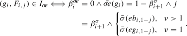
  If the corresponding conditions are fulfilled, then . Otherwise, .

We also use the following statement for comparing valuations of cycle centers.

Lemma 14

Let $G_n=M_n$. Let $\sigma \in \varLambda _{\iota }$ be a Phase-k-strategy, $k\in \{1,\dots ,5\}$, for some $\mathfrak {b}\in \mathcal {B}_n$ having Property Usv1$_i$ and Property Bac1$_{i+1}$ for some $i\in \{1,\dots ,n\}$. If $F_{i,0}$ and $F_{i,1}$ are in the same state and if either $i\ge \nu$ or $\sigma$ has Property Rel1, then $\varXi _{\sigma }^\mathrm {M}(F_{i,\beta ^{\sigma }_{i+1}})>\varXi _{\sigma }^\mathrm {M}(F_{i,1-\beta ^{\sigma }_{i+1}})$.

We now prove that we obtain a canonical strategy $\sigma _{\mathfrak {b}+1}$ for $\mathfrak {b}+1$.

Lemma 11

Let $\sigma _{\mathfrak {b}}\in \varLambda _{\iota }$ be a canonical strategy for $\mathfrak {b}$ fulfilling the canonical conditions. Then, applying improving switches according to Zadeh’s pivot rule and our tie-breaking rule produces a canonical strategy $\sigma _{\mathfrak {b}+1}\in \varLambda _{\iota }$ for $\mathfrak {b}+1$ with $I_{\sigma _{\mathfrak {b}+1}}=\{(d_{i,j,k},F_{i,j}):\sigma _{\mathfrak {b}+1}(d_{i,j,k})\ne F_{i,j}\}$.

Proof

By Lemma 10, applying improving switches according to Zadeh’s pivot rule and our tie-breaking rule yields a Phase-5-strategy $\sigma ^{(5)}$ for $\mathfrak {b}$ with $\sigma ^{(5)}\in \varLambda _{\iota }$ and $\mu ^{\sigma ^{(5)}}=u=\min \{i:\beta ^{\sigma ^{(5)}}_i=0\}$. Let $m{:}{=}\max \{i:\beta ^{\sigma }_i=1\}$ and $\sigma {:}{=}\sigma ^{(5)}$.

Consider the case $\nu =1$. We first investigate the occurrence record of the improving switches.

• 1. Let $e=(d_{i,j,k},F_{i,j})$ resp. $e=(e_{i,j,k},g_1)$ with $\sigma (e_{i,j,k})=b_2$. Then $\phi ^{\sigma }(e)=\lfloor \frac{\mathfrak {b}+1}{2}\rfloor$ by Lemma 10 resp. $\phi ^{\sigma ^{(5)}}(e)=\phi ^{\sigma _{\mathfrak {b}}}(e)=\lceil \frac{\mathfrak {b}}{2}\rceil =\lfloor \frac{\mathfrak {b}+1}{2}\rfloor$.

• 2. Let $e=(d_{i,j,k},F_{i,j})$ with $\beta ^{\sigma }_i=0, i\in \{u+1,\dots ,m-1\}$ and $j=1-\beta ^{\sigma }_{i+1}$. Then, $\mathfrak {b}_i=0$ and $j=1-\mathfrak {b}_{i+1}$ since $i\ge u+1>1$ and $\nu =1$. In addition, $\mathfrak {b}_1=0$ and, due to $i>u$, there is at least one $l\in \{2,\dots ,i-1\}$ with $(\mathfrak {b}+1)_l=\mathfrak {b}_l=0$. Consequently, Lemma 7 yields $\ell ^{\mathfrak {b}}(i,j,k)=\lceil \frac{\mathfrak {b}-2^{i-1}+\sum (\mathfrak {b},i)+1-k}{2}\rceil \le \lceil \frac{\mathfrak {b}-3-k}{2}\rceil =\left\lfloor \frac{\mathfrak {b}-k}{2}\right\rfloor -1$. Since there is a $t_{\mathfrak {b}}$ feasible for $\mathfrak {b}$, it holds that $\phi ^{\sigma _{\mathfrak {b}}}(e)=\min (\left\lfloor \frac{\mathfrak {b}+1-k}{2}\right\rfloor ,\ell ^{\mathfrak {b}}(i,j,k)+t_{\mathfrak {b}})$. We thus distinguish the following cases.

  • (a) Assume $\phi ^{\sigma _{\mathfrak {b}}}(e)=\ell ^{\mathfrak {b}}(i,j,k)+1$. Then, by Property Or2$_{i,j,k}$, $\sigma _{\mathfrak {b}}(d_{i,j,k})=F_{i,j}$ and e was not applied yet. Consequently, Property Or1$_{i,j,k}$ implies $\phi ^{\sigma }(e)=\phi ^{\sigma _{\mathfrak {b}}}(e)<\mathfrak {m}$.

  • (b) Assume $\phi ^{\sigma _{\mathfrak {b}}}(e)=\ell ^{\mathfrak {b}}(i,j,k)$. Then, $\phi ^{\sigma _{\mathfrak {b}}}(e)\le \phi ^{\sigma }(e)\le \left\lfloor \frac{\mathfrak {b}-k}{2}\right\rfloor -1<\mathfrak {m}$ as well as $\sigma _{\mathfrak {b}}(d_{i,j,k})\ne F_{i,j}$ by Property Or2$_{i,j,k}$. This implies $\phi ^{\sigma _{\mathfrak {b}}}(e)=\mathfrak {m}-1$ by Property Or4$_{i,j,k}$. Hence, by Corollary 1, e was applied during Phase 1. Consequently, $\phi ^{\sigma }(e)=\phi ^{\sigma _{\mathfrak {b}}}(e)+1=\mathfrak {m}$.

  • (c) The case $\phi ^{\sigma _{\mathfrak {b}}}(e)=\ell ^{\mathfrak {b}}(i,j,k)-1$ cannot occur since $t_{\mathfrak {b}}=-1$ is not feasible as $\mathfrak {b}$ is even.

  • (d) Assume $\phi ^{\sigma _{\mathfrak {b}}}(e)=\left\lfloor \frac{\mathfrak {b}+1-k}{2}\right\rfloor$ and $\lfloor \frac{\mathfrak {b}+1-k}{2}\rfloor \ne \ell ^{\mathfrak {b}}(i,j,k)$ and $\lfloor {\frac{\mathfrak {b}+1-k}{2}}\rfloor \ne \ell ^{\mathfrak {b}}(i,j,k)+1$. This implies $\left\lfloor \frac{\mathfrak {b}+1-k}{2}\right\rfloor <\ell ^{\mathfrak {b}}(i,j,k)$ since $\phi ^{\sigma _{\mathfrak {b}}}(e)=\min (\left\lfloor \frac{\mathfrak {b}+1-k}{2}\right\rfloor ,\ell ^{\mathfrak {b}}(i,j,k)+t_{\mathfrak {b}})$. But this is a contradiction since $\ell ^{\mathfrak {b}}(i,j,k)\le \left\lfloor \frac{\mathfrak {b}-k}{2}\right\rfloor -1.$

Thus, the occurrence records of all improving switches are bounded by $\lfloor \frac{\mathfrak {b}+1}{2}\rfloor$ and some switches have an occurrence record of exactly $\lfloor \frac{\mathfrak {b}+1}{2}\rfloor$. Consequently, improving switches $(d_{i,j,k},F_{i,j})$ with $i\in \{u+1,\dots ,m-1\}, \beta ^{\sigma }_i=0$ and $j=1-\beta ^{\sigma }_{i+1}$ are applied first. Further note that an edge $e=(d_{i,j,k},F_{i,j})$ can only fulfill these assumptions if $\sigma _{\mathfrak {b}}(d_{i,j,k})=F_{i,j}$, implying that e was not applied during Phase 1. It furthermore implies $\phi ^{\sigma }(e)=\phi ^{\sigma _{\mathfrak {b}}}(e)=\ell ^{\mathfrak {b}}(i,j,k)+1$. Consider such an edge e and assume $\phi ^{\sigma }(e)<\mathfrak {m}$. We show that row 1 of Table 11 applies to e. We thus prove $\sigma (b_i)=b_{i+1}, j=1-\beta ^{\sigma }_{i+1}, {\bar{\sigma }}(g_i)=1-\beta ^{\sigma }_{i+1}$ and $i\ne 1$. The first two statements follow directly since $\sigma$ is a Phase-5-strategy and $\beta ^{\sigma }_i=0$ as well as by the choice of j. Also, $i\ne 1$ follows from $i\ge u+1>1$. It thus suffices to show ${\bar{\sigma }}(g_i)=1-\beta ^{\sigma }_{i+1}$.

This can be shown by using Corollaries 2 and 1.$^{3}$ Hence, let $e=(d_{i,j,k},F_{i,j})\in I_{\sigma }$ be an improving switch minimizing the occurrence record. Then, $\sigma [e]$ is a Phase-5-strategy for $\mathfrak {b}$ with and by row 1 of Table 11. By Lemma 6 and the choice of i and j, $\ell ^{\mathfrak {b}}(i,j,k)+1=\ell ^{\mathfrak {b}+1}(i,j,k)$. In particular,

$$\begin{aligned} \phi ^{\sigma '}(e)=\ell ^{\mathfrak {b}}(i,j,k)+1+1=\ell ^{\mathfrak {b}+1}(i,j,k)+1\le \mathfrak {m}\le \left\lfloor \frac{(\mathfrak {b}+1)+1-k}{2}\right\rfloor . \end{aligned}$$

Thus, by choosing the parameter $t_{\mathfrak {b}+1}=1$, which is feasible since $i\ne 1$, the occurrence record of e is described by Table 2 when interpreted for $\mathfrak {b}+1$.

Now, the same arguments can be used for all improving switches $e'\in \mathbb {D}^1\cap I_{\sigma '}$ having an occurrence record smaller than $\mathfrak {m}$. All of these switches are thus applied and their occurrence records are specified by Table 2 when interpreted for $\mathfrak {b}+1$. After the application of these switches, we obtain a Phase-5-strategy $\sigma$ for $\mathfrak {b}$ with $\sigma \in \varLambda _{\iota }$ and

(2)

In particular, all improving switches have an occurrence record of $\mathfrak {m}$. Thus, the tie-breaking rule now applies a switch of the type $(e_{*,*,*},g_1)$. Let $e=(e_{i,j,k},g_1)$ denote the switch applied next. We prove that Lemma 13 applies to this switch. First, we show that $F_{i,j}$ is mixed. Since $e=(e_{i,j,k},g_1)\in I_{\sigma }$ implies $(d_{i,j,k},F_{i,j})\in I_{\sigma }$, we have ${\bar{\sigma }}(eb_{i,j})$. In particular, $F_{i,j}$ is not closed, so $\beta ^{\sigma }_{i}=0\vee \beta ^{\sigma }_{i+1}\ne j$. Consequently, $(i,j)\in S_3$ or $(i,j)\in S_4$. By Lemma 10, ${\bar{\sigma }}(eb_{i,j})$, and as no improving switch $(e_{*,*,*},b_2)$ was applied during $\sigma ^{(5)}\rightarrow \sigma$, we need to have $(i,j)\in S_3$, implying the statement. We now prove that $j=1$ implies $\lnot {\bar{\sigma }}(eb_{i,1-j})$ if $G_n=S_n$. Since $j=1$, we need to prove $\lnot {\bar{\sigma }}(eb_{i,0})$. If $F_{i,0}$ is closed, then the statement follows. If $F_{i,0}$ is not closed, then $\beta ^{\sigma }_i=0\vee \beta ^{\sigma }_{i+1}\ne j$ as $F_{i,1}$ cannot be closed by the choice of e. Consequently, $(i,0)\in S_3$ or $(i,0)\in S_4$. In the second case, $\lnot {\bar{\sigma }}^5(eb_{i,0})$ by Lemma 10 and the statement follows as no improving switch $(e_{*,*,*},b_2)$ was applied during $\sigma ^{(5)}\rightarrow \sigma$. Consider the case $(i,0)\in S_3$. Then, by Lemma 10, $F_{i,0}$ and $F_{i,1}$ are mixed with respect to $\sigma ^{(5)}$. Thus, as we consider the case $G_n=S_n$, the tie-breaking rule must have applied the improving switches $(e_{i,0,*},g_1)$ prior to $(e_{i,1,k},g_1)$, implying the statement. Note that “$j=1-\beta ^{\sigma }_{i+1}\implies \lnot {\bar{\sigma }}(eb_{i,1-j})$ if $G_n=M_n$” follows by the same arguments and since the tie-breaking rule applies improving switches $(e_{i,\beta ^{\sigma }_{i+1},*},g_1)$ first.

These arguments can be applied for any improving switch $(e_{*,*,*},g_1)$. Thus, Lemma 13 applies to the switch e. Observe that is specified by Table 2 when interpreted for $\mathfrak {b}+1$ as $\nu =1$ implies $\lceil \frac{\mathfrak {b}}{2}\rceil +1=\lceil \frac{\mathfrak {b}+1}{2}\rceil$. If the conditions listed in the fourth case of Lemma 13 are fulfilled, then . If these conditions are not fulfilled, then . In particular, $\tilde{e}{:}{=}(d_{i,j,1-k},F_{i,j})$ becomes improving in either case. We prove that $\tilde{e}$ has an occurrence record of $\mathfrak {m}$ or $\mathfrak {m}+1$.

By the characterization of $I_{\sigma }$, we have $(d_{i,j,k},F_{i,j})\in I_{\sigma }$, implying . Since $\sigma$ is a Phase-5-strategy for $\mathfrak {b}$, this implies $\beta ^{\sigma }_i=0\vee \beta ^{\sigma }_{i+1}\ne j$. Assume that $\tilde{e}$ was applied previously in this transition. It is not possible that $\tilde{e}$ was applied during Phase 5 since this would imply , contradicting that $F_{i,j}$ is mixed. Consequently, $\tilde{e}$ was applied during Phase 1. Thus, $\sigma _{\mathfrak {b}}(d_{i,j,1-k})\ne F_{i,j}$ and $\phi ^{\sigma _{\mathfrak {b}}}(\tilde{e})\in \{\mathfrak {m}-1,\mathfrak {m}\}$ by Property Or4$_{i,j,1-k}$. This implies as claimed. Now assume that $\tilde{e}$ was not applied previously, implying . Consider the case $\sigma _{\mathfrak {b}}(d_{i,j,1-k})\ne F_{i,j}$. Then, by Property Or4$_{i,j,1-k}$, $\phi ^{\sigma _{\mathfrak {b}}}(\tilde{e})\in \{\mathfrak {m}-1,\mathfrak {m}\}$. But this implies $\phi ^{\sigma _{\mathfrak {b}}}(\tilde{e})=\mathfrak {m}$ by Corollary 1 as claimed. Thus assume $\sigma _{\mathfrak {b}}(d_{i,j,1-k})=F_{i,j}$. Then, by Property Or1$_{i,j,1-k}$ and Property Or2$_{i,j,1-k}$, we have $\phi ^{\sigma _{\mathfrak {b}}}(\tilde{e})=\ell ^{\mathfrak {b}}(i,j,1-k)+1<\mathfrak {m}.$ Using Lemma 7 and by distinguishing between the cases , and , it is easy to verify that this always yields a contradiction.$^{3}$ We thus have just proven the following.

Corollary 8

If the edge $(d_{i,j,1-k},F_{i,j})$ becomes improving during Phase 5 due to the application of $(e_{i,j,k},g_1)$, then the corresponding strategy has Property Or4$_{i,j,1-k}$.

Now, assume that $(g_i,F_{i,j})$ becomes improving when applying $(e_{i,j,k},g_1)$. Using the conditions stated in Lemma 13, Corollary 2 and Lemma 10, it is easy to verify that .$^{3}$

Since , we have by Table 2. As argued previously, . Therefore, the occurrence record of any improving switch except $(g_i,F_{i,j})$ is at least $\mathfrak {m}$. Thus, $(g_i,F_{i,j})$ either uniquely minimizes the occurrence record or has the same occurrence record as all other improving switches. Consequently, by the tie-breaking rule, $(g_i,F_{i,j})$ is applied next in either case.

We prove that row 2 of Table 11 applies to this switch. Since and , it suffices to prove . But this follows as we applied $(e_{i,j,k},g_1)$ earlier and since $F_{i,j}$ was mixed when this switch was applied. Observe that the following corollary holds due to the conditions which specify when a switch $(g_i,F_{i,j})$ is unlocked, independent on $\nu$.

Corollary 9

If an improving switch $(g_i,F_{i,j})$ is applied during Phase 5, then the created strategy has Property Sv1$_i$.

Let $\sigma$ denote the strategy obtained after applying $(e_{i,j,k},g_1)$ and (eventually) $(g_i,F_{i,j})$. For now, assume that there are indices $i',j',k'$ with $(e_{i',j',k'},g_1)\in I_{\sigma }$. Then, by Lemma 13 resp. row  2 of Table 11, $\sigma$ is a Phase-5-Strategy for $\mathfrak {b}$. By our previous discussion, all improving switches have an occurrence record of at least $\mathfrak {m}$. Among all improving switches with an occurrence record of exactly $\mathfrak {m}$, the tie-breaking rule then decides which switch to apply. There are two types of improving switches. Each switch is either of the form $(d_{i,j,k},F_{i,j})$ or of the form $(e_{i,j,k},g_1)$ with $\sigma (d_{i,j,k})=e_{i,j,k}$. Since every edges $(e_{i,j,k},g_1)$ minimizes the occurrence record among all improving switches, one of these edges is chosen. But then, the same arguments used previously can be used again. More precisely, Lemma 13 applies to this switch, making the edge $(d_{i,j,1-k},F_{i,j})$ and eventually also $(g_i,F_{i,j})$ improving. Also, Corollaries 8 and 9 apply to these switches and another switch of the form $(e_{*,*,*},g_1)$ is applied afterwards. Thus, inductively, all remaining switches of the form $(e_{i,j,k},g_1)$ are applied.

Each of these applications creates the improving switch $(d_{i,j,1-k},F_{i,j})$ and might make $(g_i,F_{i,j})$ improving. In the latter case, the corresponding switch is then applied immediately. Let $\sigma$ denote the strategy that is reached before the last improving switch of the form $(e_{*,*,*},g_1)$ is applied. We argue that this switch is $e\,{:}{=}\,(e_{1,1-\beta ^{\sigma }_2,k},g_1)$ for some $k\in \{0,1\}$ and that $\sigma$ has Property Sv1$_{i}$ for all $i\in \{1,\dots ,n\}$. As the tie-breaking rule applies improving switches in higher levels first, it suffices to prove that there there is a $k\in \{0,1\}$ such that $e\in I_{\sigma ^{(5)}}$. This however follows from Lemma 10 as $\nu =1$ implies $(1,\beta ^{\sigma }_2)\in S_3$. It remains to prove that $\sigma$ has Property Sv1$_{i}$ for all $i\in \{1,\dots ,n\}$. If $\beta ^{\sigma }_i=1$, then this follows from the definition of a Phase-5-strategy. If $\beta ^{\sigma }_i=0$ and $(g_i,F_{i,j})\in \mathfrak {A}_{\sigma ^{(5)}}^{\sigma }$, then this follows from Corollary 9. Thus, let $\beta ^{\sigma }_i=0$ and $(g_i,F_{i,j})\notin \mathfrak {A}_{\sigma ^{(5)}}^{\sigma }$, implying $i\ne 1$ since $\nu =1$. We now prove the following statemen. If ${\bar{\sigma }}(g_i)=1$ (if $G_n=S_n$) resp. ${\bar{\sigma }}(g_i)=1-\beta ^{\sigma }_{i+1}$ (if $G_n=M_n$) and $\lnot {\bar{\sigma }}(d_{i,1})$ (if $G_n=S_n$), resp. $\lnot {\bar{\sigma }}(d_{i,1-\beta ^{\sigma }_{i+1}})$ (if $G_n=M_n$), then $(g_i,F_{i,0})\in I_{\sigma }$ resp. $(g_i,F_{i,\beta ^{\sigma }_{i+1}})\in I_{\sigma }$. Note that this proves the statement as $I_{\sigma }\cap \mathbb {G}=\emptyset$.

Thus, let $j\,{:}{=}\, 0$ (if $G_n=S_n$) resp. $j{:}{=}\beta ^{\sigma }_{i+1}$ (if $G_n=M_n$) and assume $\lnot {\bar{\sigma }}(d_{i,1-j})$. It suffices to prove $\varXi _{\sigma }^*(F_{i,j})\succ \varXi _{\sigma }^*(F_{i,1-j})$. As $\sigma (e_{i',j',k'})=g_1$ for all $(i',j',k')\ne (1,\beta ^{\sigma }_2,k), i\ne 1$ and $\mu ^{\sigma }=u\ne 1$, the cycle centers are either closed or escape only to $g_1$. Note that a closed cycle center has $\varXi _{\sigma }^*(F_{i,j})=\varXi _{\sigma }^*(s_{i,j})$ due to Lemma 1. Let $G_n=S_n$. If both cycle centers escape towards $g_1$, then the statement follows since

due to the priorities of $F_{i,0}$ and $F_{i,1}$. As $\beta ^{\sigma }_i=0$, only $F_{i,1-\beta ^{\sigma }_{i+1}}$ can be closed. Assume that we have $j=0=1-\beta ^{\sigma }_{i+1}$. Then, by Property Usv1$_i$ and since $\sigma (b_1)=g_1$, the statement follows since $\varXi _{\sigma }^\mathrm {S}(F_{i,0})=\{s_{i,0},b_1\}\cup \varXi _{\sigma }^\mathrm {S}(g_1)$ and for some $k\in \{0,1\}$. Now assume $j=0=\beta ^{\sigma }_{i+1}$. Then, $F_{i,1-j}=F_{i,1}$ is closed, contradicting the assumption of the statement. Let $G_n=M_n$. If both cycle centers are $g_1$-open or $g_1$-halfopen, then the statement follows by Lemma 14 since $i>\nu$. If one of the cycle centers is $g_1$-open and one cycle center is $g_1$-halfopen, then the statement follows by an easy calculation.$^{3}$ Since only $F_{i,1-\beta ^{\sigma }_{i+1}}=F_{i,1-j}$ can be closed in level i, the statement then follows by the same argument used for the case $G_n=S_n$.

Thus, Lemma 13 applies to $(e_{1,\beta ^{\sigma }_2,k},g_1)$. Let . Then, by Lemma 13, $\sigma _{\mathfrak {b}+1}$ is a Phase-1-strategy for $\mathfrak {b}+1$ with $\sigma _{\mathfrak {b}+1}\in \varLambda _{\iota }$. Note that, since every edge was applied at most once during $\sigma _{\mathfrak {b}}\rightarrow \sigma ^{(5)}$ by Lemma 10 and since no edge applied during $\sigma ^{(5)}\rightarrow \sigma _{\mathfrak {b}+1}$ was applied earlier, every edge was applied at most once as improving switch during $\sigma _{\mathfrak {b}}\rightarrow \sigma _{\mathfrak {b}+1}$. Also note that we implicitly proved the following corollary.

Corollary 10

Let $\nu =1$ and let $\sigma _{\mathfrak {b}+1}$ denote the strategy obtained after the application of the final improving switch $(e_{*,*,*},g_1)$. Then $(d_{i,j,k},F_{i,j})\in \mathfrak {A}_{\sigma ^{(5)}}^{\sigma _{\mathfrak {b}+1}}$ if and only if $\sigma _{\mathfrak {b}}(d_{i,j,k})=F_{i,j}, \phi ^{\sigma _{\mathfrak {b}}}(d_{i,j,k},F_{i,j})<\mathfrak {m}, i\in \{u+1,\dots ,m-1\}, \beta ^{\sigma _{\mathfrak {b}+1}}_i=0$ and $j=1-\beta ^{\sigma _{\mathfrak {b}+1}}_{i+1}$. In addition, $\sigma _{\mathfrak {b}+1}$ has Property Or2$_{i,j,k}$

We prove that $\sigma _{\mathfrak {b}+1}$ is a canonical strategy for $\mathfrak {b}+1$ with $I_{\sigma _{\mathfrak {b}+1}}=\mathfrak {D}^{\sigma _{\mathfrak {b}+1}}$. To simplify notation, let $\sigma {:}{=}\sigma _{\mathfrak {b}+1}$. We first prove$I_{\sigma }=\{(d_{i,j,k},F_{i,j}):\sigma (d_{i,j,k})\ne F_{i,j}\}$. Consider the strategy $\sigma ^{(5)}$. Using the characterization of the strategy that was obtained after having applied all switches $(d_{i,j,k},F_{i,j})$ with an occurrence record smaller than $\mathfrak {m}$ (see Eq. (2)), we obtain

In particular, $I_{\sigma }\subseteq \{(d_{i,j,k},F_{i,j}):\sigma (d_{i,j,k})\ne F_{i,j}\}$ and every improving switch has an occurrence record of at least $\mathfrak {m}$. To prove $\{(d_{i,j,k},F_{i,j}):\sigma (d_{i,j,k})\ne F_{i,j}\}\subseteq I_{\sigma }$, let $e{:}{=}(d_{i,j,k},F_{i,j})$ with $\sigma (d_{i,j,k})\ne F_{i,j}$. It thus suffices to show $\varXi _{\sigma }^*(F_{i,j})\succ \varXi _{\sigma }^*(e_{i,j,k})$. Property Esc1 and $\nu =1$ imply ${\bar{\sigma }}(eg_{i,j})\wedge \lnot {\bar{\sigma }}(eb_{i,j})$. Furthermore, $\mu ^{\sigma }=\min \{i':\sigma (b_{i'})=b_{i'+1}\}\ne 1$ as $\sigma$ has Property Rel1. It is easy to verify that this implies $\varXi _{\sigma }^\mathrm {S}(F_{i,j})=\{F_{i,j}\}\cup \varXi _{\sigma }^\mathrm {S}(e_{i,j,k})$, hence $\varXi _{\sigma }^\mathrm {S}(F_{i,j})\rhd \varXi _{\sigma }^\mathrm {S}(e_{i,j,k})$. For $G_n=M_n$, it suffices to prove $\varXi _{\sigma }^{\mathrm {M}}(s_{i,j})>\varXi _{\sigma }^{\mathrm {M}}(g_1)$ as this implies $\varXi _{\sigma }^{\mathrm {M}}(F_{i,j})>\varXi _{\sigma }^{\mathrm {M}}(g_1)$. Since $\sigma (d_{i,j,k})\ne F_{i,j}$, either $\beta ^{\sigma }_i=0$ or $\beta ^{\sigma }_{i+1}\ne j$. In the second case, Property Usv1$_i$ implies that we have $\sigma (s_{i,j})=b_1$ and the statement follows since $\varXi _{\sigma }^{\mathrm {M}}(s_{i,j},b_1)=\langle s_{i,j}\rangle +\varXi _{\sigma }^{\mathrm {M}}(g_1)$ due to $\sigma (b_1)=g_1$. Thus assume $\beta ^{\sigma }_i=0\wedge \beta ^{\sigma }_{i+1}=j$. Then, the statement follows since $\varXi _{\sigma }^{\mathrm {M}}(s_{i,j})=\langle s_{i,j},h_{i,j}\rangle +\varXi _{\sigma }^{\mathrm {M}}(b_{i+1})$ by Property Bac1$_{i+1}$ and since $\langle s_{i,j},h_{i,j}\rangle >\sum _{\ell <i}\langle g_\ell ,s_{\ell ,{\bar{\sigma }}(g_{\ell })},h_{\ell ,{\bar{\sigma }}(g_{\ell })}\rangle$.

We now prove that $\sigma$ is a canonical strategy for $\mathfrak {b}+1$. Since $\sigma$ is a Phase-1-strategy for $\mathfrak {b}+1$, we have $\mathfrak {b}+1=\beta ^{\sigma }$. Consider the conditions listed in Definition 2 resp. 4. Condition 1 is fulfilled since $\sigma (e_{*,*,*})=g_1$ and $\nu =1$. Condition 2(a) is fulfilled since $\beta ^{\sigma }_i=(\mathfrak {b}+1)_i=1$ implies $\sigma (b_i)=g_i$ by Property Bac1$_i$. Consider condition 2(b). If $(\mathfrak {b}+1)_i=1$, then $F_{i,(\mathfrak {b}+1)_{i+1}}$ is closed by Property Bac1$_i$. It is easy to verify that $(\mathfrak {b}+1)_{i}=1$ implies that $F_{i,1-(\mathfrak {b}+1)_{i+1}}$ cannot be closed, hence Condition 2(b) is fulfilled.$^{3}$ Condition 2(c) is fulfilled by $\beta ^{\sigma }=\mathfrak {b}+1$ and Property Bac2$_*$. Conditions 3(a) and 3(b) are fulfilled since $\sigma$ has Property Bac1$_*$. Consider condition 3(c). We prove that $(\mathfrak {b}+1)_i=0$ and ${\bar{\sigma }}(d_{i,j})$ imply $\sigma (g_{i})=F_{i,j}$ where $j=1-(\mathfrak {b}+1)_{i+1}$. By Lemma 1, $F_{i,j}$ being closed implies ${\hat{\varXi }}_{\sigma }^*(F_{i,j})={\hat{\varXi }}_{\sigma }^*(s_{i,j})$. Thus, $\varXi _{\sigma }^*(F_{i,j})=[\![{s_{i,j}}]\!]\oplus \varXi _{\sigma }^*(g_1)$ by the choice of j and since $\nu =1$. It can be shown that $\mu ^{\sigma }\ne 1, {\bar{\sigma }}(eg_{i,1-j}), \lnot {\bar{\sigma }}(eb_{i,1-j})$ and $1-j=\beta ^{\sigma }_{i+1}$ implies $\varXi _{\sigma }^*(F_{i,1-j})=\{F_{i,1-j}, d_{i,1-j,k}, e_{i,1-j,k}, b_1\}\cup \varXi _{\sigma }^*(g_1)$ for some $k\in \{0,1\}$.$^{3}$ But this implies $\sigma (g_i)=F_{i,j}$ since $(g_i,F_{i,1-j})\in I_{\sigma }$ otherwise, contradicting $I_{\sigma }=\{(d_{i,j,k},F_{i,j}):\sigma (d_{i,j,k})=F_{i,j}\}$.

Consider condition 3(d) and let $j{:}{=}0$ if $G_n=S_n$ and $j{:}{=}\beta ^{\sigma }_{i+1}$ if $G_n=M_n$. It suffices to prove $\varXi _{\sigma }^*(F_{i,j})\succ \varXi _{\sigma }^*(F_{i,1-j})$ if none of the cycle centers is closed. For $G_n=M_n$, this follows from Lemma 14 or an easy calculation if $G_n=M_n$ since $i\ge 1=\nu$. For $G_n=S_n$, this follows from $\varOmega (F_{i,0})>\varOmega (F_{i,1})$ and since both priorities are even. Conditions 4 and 5 follow as $\sigma$ has Property Usv1$_{*}$. For condition 6, let $i{:}{=}\nu (\mathfrak {b}+2), j{:}{=}(\mathfrak {b}+1)_{i+1}$ and $k\in \{0,1\}$. Since $\nu (\mathfrak {b}+1)=1$, we have $i\ge 2$ and $\mathfrak {b}_i=(\mathfrak {b}+1)_i=0$ as well as $\mathfrak {b}_{i+1}=(\mathfrak {b}+1)_{i+1}=j$. We prove $\sigma (d_{i,j,k})\ne F_{i,j}$. For the sake of contradiction, let $\sigma (d_{i,j,k})=F_{i,j}$. Then, by the choice of i and j and Lemma 10, $(d_{i,j,k},F_{i,j})\in \mathfrak {A}_{\sigma ^{(5)}}^{\sigma }$. Thus, by Corollary 10 and Property Or2$_{i,j,k}$, it holds that $\phi ^{\sigma ^{(5)}}(d_{i,j,k},F_{i,j})<\mathfrak {m}$ and $\phi ^{\sigma _{\mathfrak {b}}}(d_{i,j,k},F_{i,j})=\ell ^{\mathfrak {b}}(i,j,k)+1$. But, by Lemma 7, we have $\ell ^{\mathfrak {b}}(i,j,k)=\lceil \frac{\mathfrak {b}+2^{i-1}+\sum (\mathfrak {b},i)+1-k}{2}\rceil \ge \lceil \frac{\mathfrak {b}+3-k}{2}\rceil =\lfloor \frac{\mathfrak {b}+2-k}{2}\rfloor$, which is a contradiction. Hence, $\sigma (d_{i,j,k})\ne F_{i,j}$.

Now consider the case ${\varvec{\nu }}>\mathbf{1}$. Then, $\mathfrak {b}$ is odd and $\mathfrak {m}=\left\lfloor \frac{\mathfrak {b}}{2}\right\rfloor +1$. By Lemma 10, applying improving switches according to Zadeh’s pivot rule and our tie-breaking rule yields a Phase-5-strategy $\sigma$ for $\mathfrak {b}$ with $\sigma \in \varLambda _{\iota }$ and $\mu ^{\sigma }=u$. In addition

where, $X_k$ is defined as in Table 7. We now investigate the occurrence records of the improving switches. Note that $\varXi _{\sigma }^*(g_1)\prec \varXi _{\sigma }^*(b_2)$ since $\sigma (e_{i,j,k})=g_1$ implies $(e_{i,j,k},b_2)\in I_{\sigma }$.

• 1. Let $e=(d_{i,j,k},F_{i,j})$ with $\sigma (e_{i,j,k})=g_1$. Then, by Lemma 10, $\phi ^{\sigma }(e)=\phi ^{\sigma _{\mathfrak {b}}}(e)=\mathfrak {m}$.

• 2. Let $e=(e_{i,j,k},b_2)$ with $\sigma (e_{i,j,k})=g_1$. Then, by Table 2, $\phi ^{\sigma }(e)=\phi ^{\sigma _{\mathfrak {b}}}(e)=\left\lfloor \frac{\mathfrak {b}}{2}\right\rfloor =\mathfrak {m}-1.$

• 3. Let $e=(d_{\nu ,j,k},F_{\nu ,j})$ with $j{:}{=}1-\beta ^{\sigma }_{\nu +1}$ for some $k\in \{0,1\}$. This edge is only improving if $\mathfrak {b}+1$ is not a power of two. Note that this implies . Since $\mathfrak {b}_{\nu }=0\wedge \mathfrak {b}_{\nu +1}\ne j$, Lemma 7 thus implies

  $$\begin{aligned} \ell ^{\mathfrak {b}}(\nu ,j,k)={\left\{ \begin{array}{ll} \mathfrak {m}, &{}k=0\\ \mathfrak {m}-1, &{}k=1\end{array}\right. }. \end{aligned}$$

  Since $\mathfrak {b}+1$ is not a power of two, the parameter $t_{\mathfrak {b}}=-1$ is not feasible by Property Or3$_{i,j,k}$. Hence $\phi ^{\sigma _{\mathfrak {b}}}(d_{\nu ,j,k},F_{\nu ,j})=\mathfrak {m}-k$. This implies $(d_{\nu ,j,1},F_{\nu ,j})\in \mathfrak {A}_{\sigma _{\mathfrak {b}}}^{\sigma }$ by Corollary 1. Consequently, $\phi ^{\sigma }(d_{\nu ,j,k},F_{\nu ,j})=\mathfrak {m}$ for both $k\in \{0,1\}$.

• 4. Let $e=(d_{i,j,k},F_{i,j})$ with $i\in \{\nu +1,\dots ,m-1\}, \beta ^{\sigma }_i=0, j{:}{=}1-\beta ^{\sigma }_{i+1}$ and $k\in \{0,1\}$. This edge is only improving if $\mathfrak {b}+1$ is not a power of two. Since $i>\nu$, $\beta ^{\sigma }_i=0$ implies $\mathfrak {b}_i=0\wedge \mathfrak {b}_{i+1}\ne j$. Also, $i<m$ implies since $j=1-\beta ^{\sigma }_{i+1}$ and $\mathfrak {b}\ge 1$ by the choice of i. It is easy to verify that $\mathfrak {b}_{\nu }=0$ then implies $\ell ^{\mathfrak {b}}(i,j,k)\le \mathfrak {m}-1$.$^{3}$ There are two cases. If $\sigma _{\mathfrak {b}}(d_{i,j,k})=F_{i,j}$, then $\phi ^{\sigma _{\mathfrak {b}}}(d_{i,j,k},F_{i,j})=\ell ^{\mathfrak {b}}(i,j,k)+1\le \mathfrak {m}-1$ by Property Or1$_{i,j,k}$. If $\sigma _{\mathfrak {b}}(d_{i,j,k})\ne F_{i,j}$, then $\phi ^{\sigma _{\mathfrak {b}}}(d_{i,j,k},F_{i,j})=\ell ^{\mathfrak {b}}(i,j,k)\le \mathfrak {m}-1$. In the first case, e was not applied during Phase 1 and $\phi ^{\sigma _{\mathfrak {b}}}(e)=\phi ^{\sigma }(e)\le \mathfrak {m}-1$. In the second case, $\phi ^{\sigma _{\mathfrak {b}}}(e)=\mathfrak {m}-1$ by Property Or4$_{i,j,k}$. Then, e was applied during Phase 1, implying $\phi ^{\sigma }(d_{i,j,k},F_{i,j})=\mathfrak {m}$.

• 5. Let $e=(d_{i,j,k},F_{i,j})$ with $i\le \nu (\mathfrak {b}+1)-1$ and $j{:}{=}1-\beta ^{\sigma }_{i+1}$. Then, bit i and bit $i+1$ switched during $\sigma _{\mathfrak {b}}\rightarrow \sigma ^{(5)}$. In particular, $F_{i,j}$ was closed with respect to $\sigma _{\mathfrak {b}}$ and consequently $(d_{i,j,k},F_{i,j})\notin \mathfrak {A}_{\sigma _{\mathfrak {b}}}^{\sigma }$. Hence, by Table 2, $\phi ^{\sigma }(e)=\phi ^{\sigma _{\mathfrak {b}}}(e)=\left\lfloor \frac{\mathfrak {b}-2^{i-1}+3-k}{2}\right\rfloor .$ We now distinguish several cases.

  • For $i=1$, $\phi ^{\sigma }(e)=\left\lfloor \frac{\mathfrak {b}+2-k}{2}\right\rfloor =\mathfrak {m}$ independent of k.

  • For $i=2$, $\phi ^{\sigma }(e)=\left\lfloor \frac{\mathfrak {b}+1-k}{2}\right\rfloor$, so $\phi ^{\sigma }(e)=\mathfrak {m}$ if $k=0$ and $\phi ^{\sigma }(e)=\mathfrak {m}-1$ if $k=1$.

  • For $i=3$, $\phi ^{\sigma }(e)=\left\lfloor \frac{\mathfrak {b}-1-k}{2}\right\rfloor$, so $\phi ^{\sigma }(e)=\mathfrak {m}-1$ if $k=0$ and $\phi ^{\sigma }(e)=\mathfrak {m}-2$ if $k=1$.

  • For $i>3$, it is easy to see that the occurrence record is always strictly smaller than $\mathfrak {m}-1$.

We partition $I_{\sigma }$ into three subsets. A switch $e\in I_{\sigma }$ is called type 1 switch if $\phi ^{\sigma }(e)=\mathfrak {m}$, type 2 switch if $\phi ^{\sigma }(e)=\mathfrak {m}-1$ and type 3 switch if $\phi ^{\sigma }(e)<\mathfrak {m}-1$. By Zadeh’s pivot rule, type 3 switches are applied first. Thus, let $e\in I_{\sigma }$ be a type 3 switch and note that this implies $e=(d_{i,j,k},F_{i,j})$ where either $i<\nu -1, j=1-\beta ^{\sigma }_{i+1}$ or $i\in \{\nu +1,\dots ,m-1\}, \beta ^{\sigma }_i=0, j{:}{=}1-\beta ^{\sigma }_{i+1}$ as well as $\sigma _{\mathfrak {b}}(d_{i,j,k})=F_{i,j}$. In particular, by Property Or2$_{i,j,k}$, these switches fulfill $\phi ^{\sigma _{\mathfrak {b}}}(e)=\ell ^{\mathfrak {b}}(i,j,k)+1$ We prove that applying e can be described by row 1 of Table 11. Since it is easy to verify $i\ne 1$ and $\sigma (b_i)=b_{i+1}$ using the previous explanations and that any improving switch of type 3 has $\sigma (b_i)=b_{i+1}$, we only show ${\bar{\sigma }}(g_i)=1-\beta ^{\sigma }_{i+1}$. By Lemma 10, this holds for all $i\le \nu -1$. It thus suffices to prove this for $i\in \{\nu +1,\dots ,m-1\}\wedge \beta ^{\sigma }_{i}=0$. This can be shown by proving that ${\bar{\sigma }}(g_i)=\beta ^{\sigma }_{i+1}$ implies $(g_i,F_{i,1-\beta ^{\sigma }_{i+1}})\in I_{\sigma }$, contradicting the given characterization of $I_{\sigma }$.$^{3}$

Thus, all requirements for applying row 1 of Table 11 are met. We next show that Table 2 specifies the occurrence record of $e=(d_{i,j,k},F_{i,j})$ its application when interpreted for $\mathfrak {b}+1$. First let $i\in \{\nu +1,\dots ,m-1\}, \beta ^{\sigma }_i=0$ and $j=1-\beta ^{\sigma }_{i+1}$. Since e is a type 3 switch, this implies $\phi ^{\sigma _{\mathfrak {b}}}(e)=\ell ^{\mathfrak {b}}(i,j,k)+1$ as we pointed out in the previous paragraph. Since e is applied, the statement follows since $\ell ^{\mathfrak {b}+1}(i,j,k)=\ell ^{\mathfrak {b}}(i,j,k)+1$ by Lemma 9. Now let $i\le \nu -1$. Then, $F_{i,j}$ was closed with respect to $\sigma _{\mathfrak {b}}$ and $j=\mathfrak {b}_{i+1}=1-\beta ^{\sigma }_{i+1}$. It is easy to verify that this implies that we have $\phi ^{\sigma _{\mathfrak {b}}}(e)=\lceil \frac{\mathfrak {b}-\sum (\mathfrak {b},i)+1-k}{2}\rceil$. Since $(\mathfrak {b}+1)_i=0\wedge (\mathfrak {b}+1)_{i+1}\ne j$ and the switch e is applied, it suffices to prove $\ell ^{\mathfrak {b}+1}(i,j,k)=\lceil \frac{\mathfrak {b}-\sum (\mathfrak {b},i)+1-k}{2}\rceil$ as we can then choose $t^{\mathfrak {b}+1}=1$ as feasible. This however follows by an easy calculation.$^{3}$ Note that we do not discuss yet that choosing this parameter is in accordance with Properties (Or1)$_{*,*,*}$ to (Or4)$_{*,*,*}$. Note that e being a type 3 switch thus implies . Hence, has Property Or1$_{i,j,k}$.

Corollary 11

Let $\nu >1$. Every switch $e=(d_{i,j,k},F_{i,j})$ with $\phi ^{\sigma _{\mathfrak {b}}}(e)<\mathfrak {m}-1$ (i.e., every switch of type 3) is applied during Phase 5, and the obtained strategy has Property Or1$_{i,j,k}$.

Now, the first row of Table 11 and the corresponding arguments can be applied for every improving switch of type 3. Thus, we obtain a Phase-5-strategy $\sigma \in \varLambda _{\iota }$ such that any improving switch is of type 1 or 2. The next improving switch that is applied has an occurrence record of $\mathfrak {m}-1$, i.e., it is of type 2. Since any switch is either of the form $(d_{i,j,k},F_{i,j})$ or $(e_{i,j,k},b_2)$ and since the latter switches are of type 2, some switch $e=(e_{i,j,k},b_2)$ is applied next due to the tie-breaking rule. We prove that Lemma 13 describes the application of this switch. We begin by proving that $F_{i,j}$ is mixed. Since only improving switches of type 3 were applied, $\sigma (e_{i,j,k})=g_1$ implies $\sigma (d_{i,j,k})=e_{i,j,k}$. Consequently, ${\bar{\sigma }}(eg_{i,j})$. In particular, $F_{i,j}$ is not closed, so $\beta ^{\sigma }_i=0\vee \beta ^{\sigma }_{i+1}=j$. Thus, either $(i,j)\in S_1$ or $(i,j)\in S_2$. By Lemma 10, ${\bar{\sigma }}(eg_{i,j})$ and as no switch $(e_{*,*,*}, g_1)$ was applied during $\sigma ^{(5)}\rightarrow \sigma$, we need to have $(i,j)\in S_2$, implying that $F_{i,j}$ is mixed. We go on an prove that $j=1$ resp. $j=1-\beta ^{\sigma }_{i+1}$ (depending on whether $G_n=S_n$ or $G_n=M_n$) implies $\lnot {\bar{\sigma }}(eg_{i,1-j})$. Consider the case $G_n=S_n$ and thus $j=1$ first. We prove $\lnot {\bar{\sigma }}(eg_{i,0})$. If $F_{i,0}$ is closed, then the statement follows. If it is not closed, then $\beta ^{\sigma }_i=0\vee \beta ^{\sigma }_{i+1}\ne 0$. Consequently, either $(i,0)\in S_1$ or $(i,0)\in S_2$. In the first case, $\lnot {\bar{\sigma }}(eg_{i,0})$ follows from Lemma 10 as no improving switch $(e_{*,*,*}, b_2)$ was applied during $\sigma ^{(5)}\rightarrow \sigma$, so assume $(i,0)\in S_2$. Then, by Lemma 10, both cycle centers $F_{i,0}, F_{i,1}$ were mixed for $\sigma ^{(5)}$. Thus, as we consider $G_n=S_n$, the tie-breaking rule must have applied the improving switches $(e_{i,0,*},b_2)$ prior to $(e_{i,j,k},b_2)$, implying $\lnot {\bar{\sigma }}(eg_{i,0})$. If $G_n=M_n$, $\lnot {\bar{\sigma }}(eg_{i,1-j})$ follows by the same arguments as the tie-breaking rule applied the improving switches $(e_{i,\beta ^{\sigma }_{i+1},*},b_2)$ first. Finally, as no improving switch $(g_*,F_{*,*})$ was applied during $\sigma ^{(5)}\rightarrow \sigma$, $\nu =2$ implies $\sigma (g_1)=F_{1,0}$ if $G_n=S_n$ by Lemma 10.

Thus, all requirements of Lemma 13 are met. In addition, Table 2 describes the occurrence record of e when interpreted for $\mathfrak {b}+1$ since . Now, by Lemma 13, and $(g_{i},F_{i,j})$ might become improving for . The strategy is now either a Phase-5-strategy for $\mathfrak {b}$ or a Phase-1-strategy for $\mathfrak {b}+1$.By similar arguments used for proving Corollary 8, it is easy to verify the following corollary.$^{3}$

Corollary 12

If $(d_{i,j,1-k},F_{i,j})$ becomes improving during Phase 5 after the application of $(e_{i,j,k},b_2)$, then the corresponding strategy has Property Or4$_{i,j,1-k}$ and $\min _{k'\in \{0,1\}}\phi ^{\sigma _{\mathfrak {b}}}(d_{i,j,k'},F_{i,j})\le \mathfrak {m}-1$.

We now use Corollary 12 to prove that $(g_i,F_{i,j})$ is applied next if it becomes improving. Note that is a Phase-5-strategy for $\mathfrak {b}$ if such a switch is unlocked since it does not have Property Sv1$_i$ then. Let $\sigma$ denote the current strategy and note that we consider a strategy that was obtained by applying an improving switch $(e_{i,j,*},b_2)$ according to Lemma 13.

Due to the tie-breaking rule and Corollary 12, it suffices to show $\phi ^{\sigma }(g_{i},F_{i,j})\le \mathfrak {m}-1$. Since Table 2 and Corollary 12 yield $\phi ^{\sigma _{\mathfrak {b}}}(g_i,F_{i,j})\le \min _{k'\in \{0,1\}}\phi ^{\sigma _{\mathfrak {b}}}(d_{i,j,k'},F_{i,j})\le \mathfrak {m}-1$, it suffices to prove $(g_i,F_{i,j})\notin \mathfrak {A}_{\sigma _{\mathfrak {b}}}^{\sigma }$. By Lemma 13, $e\in I_{\sigma }$ if and only if $\beta ^{\sigma }_i=0, {\bar{\sigma }}(eb_{i,1-j})$ and $[j=0\wedge {\bar{\sigma }}(g_i)=1]$ if $G_n=S_n$ resp. $[j=\beta ^{\sigma }_{i+1}\wedge {\bar{\sigma }}(g_i)=1-\beta ^{\sigma }_{i+1}]$ if $G_n=M_n$. Let, for the sake of contradiction, $(g_i,F_{i,j})\in \mathfrak {A}_{\sigma _{\mathfrak {b}}}^{\sigma }$. The conditions on j and ${\bar{\sigma }}(g_i)$ imply $(g_i,F_{i,j})\notin \mathfrak {A}_{\sigma ^{(5)}}^{\sigma }$. Since $\beta ^{\sigma }_i=0$ implies $i\ne \nu$, also $(g_i,F_{i,j})\ne (g_\nu ,F_{\nu ,*})$. Thus, by Lemma 10, $\mathfrak {b}_i=0\wedge \mathfrak {b}_{i+1}\ne j$. Consequently, $0=\mathfrak {b}_i=\beta ^{\sigma }_{i+1}=(\mathfrak {b}+1)_{i+1}$ and $j=1-\mathfrak {b}_{i+1}$. Since all bits below level $\nu$ have $\mathfrak {b}_i=1\wedge (\mathfrak {b}+1)_i=0$, this implies $i>\nu$. Therefore, $\mathfrak {b}_{i+1}=(\mathfrak {b}+1)_{i+1}=1-j$ and in particular $j=1-\beta ^{\sigma }_{i+1}$ This is a contradiction if $G_n=M_n$ as $j=\beta ^{\sigma }_{i+1}$, hence consider the case $G_n=S_n$. Then, $j=1-\beta ^{\sigma }_{i+1}=0$, implying $\beta ^{\sigma }_{i+1}=1$. Thus, $i\in \{\nu +1,\dots ,m-1\}, \beta ^{\sigma }_{i}=0$ and $j=1-\beta ^{\sigma }_{i+1}$, implying $(i,j)\in S_1$. Therefore, ${\bar{\sigma }}^5(eb_{i,j})\wedge \lnot {\bar{\sigma }}^5(eg_{i,j})$, contradicting $(e_{i,j,k},b_2), (d_{i,j,k},e_{i,j,k})\in I_{\sigma ^{(5)}}$. Thus, $(g_i,F_{i,j})\notin \mathfrak {A}_{\sigma _{\mathfrak {b}}}^{\sigma ^{(5)}}$, implying $\phi ^{\sigma }(g_i,F_{i,j})\le \mathfrak {m}-1$.

Due to the tie-breaking rule, $(g_i,F_{i,j})$ is thus applied next. We prove that the row 2 of Table 10 applies to our situation.

First, $\beta ^{\sigma }_i=0$ follows from the conditions of Lemma 13. Second, ${\bar{\sigma }}(eb_{i,j})\wedge \lnot {\bar{\sigma }}(eg_{i,j})$ follows as the cycle center $F_{i,j}$ was mixed earlier and since we just applied $(e_{i,j,k},b_2)$. To prove that we have ${\bar{\sigma }}(d_{i',j'})\vee [{\bar{\sigma }}(eb_{i',j'})\wedge \lnot {\bar{\sigma }}(eg_{i',j'})]$ holds for all $i'\ge i$ and $j\in \{0,1\}$, fix some $i'\ge i$ and $j'\in \{0,1\}$. If $\beta ^{\sigma }_{i'}=1\wedge \beta ^{\sigma }_{i'+1}=j'$, the statement follows from Property Bac1$_{i'}$. We may hence assume $\beta ^{\sigma }_{i'}=0\vee j'\ne \beta ^{\sigma '}_{i+1}$ and that $F_{i',j'}$ is not closed. Then, by Lemma 10, either ${\bar{\sigma }}(eb_{i',j'})\wedge {\bar{\sigma }}(eg_{i',j'})$ or ${\bar{\sigma }}(eb_{i',j'})\wedge \lnot {\bar{\sigma }}(eg_{i',j'})$. Assume, for the sake of contradiction, that the first case was true and note that this implies $i'\ne i$. Then, for some $k\in \{0,1\}$, $\sigma (e_{i',j',k})=g_1$ and $\sigma (d_{i',j',k})=e_{i',j',k}$. This in particular implies $(e_{i',j',k},b_2)\in I_{\sigma }$. This is however a contradiction to the fact that we apply improving switches according to the tie-breaking rule since $i'> i$ implies that the switch $(e_{i',j',k},b_2)$ is applied before the switch $(e_{i,j',k},b_2)$.

Hence, all requirements of the second row of Table 10 are met and the statement can be applied. Further note that the strategy obtained after applying the switch has Property Sv1$_i$ due to the conditions described in Lemma 13. In particular, Corollary 9 also holds for $\nu >1$.

After the application of $(e_{i,j,k},b_2)$ (or $(g_i,F_{i,j})$ if it becomes improving), the tie-breaking rule determines which switch is applied next. Since $(d_{i,j,1-k},F_{i,j})$ has an occurrence record of at least $\mathfrak {m}-1$, another switch of the type $(e_{*,*,*},b_2)$ is applied. But then, the same arguments used above can be used again. That is, we can apply some switch $(e_{i',j',k'},b_2)$, making $(d_{i',j',1-k'},F_{i',j'})$ improving, and eventually making $(g_{i'},F_{i',j'})$ improving as well. The switch $(g_{i'}, F_{i',j'})$ is applied immediately (if it becomes improving) whereas the other switch is not applied. Then, inductively, all remaining switches of the form $(e_{*,*,*},b_2)$ are applied.

Let $\sigma$ denote the strategy that is reached after applying the final improving switch $(e_{i,j,k},b_2)$. We can then show that Property Sv1$_i$ holds for all $i\ge 2$. Furthermore, if $(g_1,F_{1,j})$ does not become improving, it is easy to prove that Property Sv1$_1$ holds at well.$^{3}$ The same is true after the application of this switch if it becomes improving. In any case, we obtain a strategy that has Property Sv1$_i$ for all $i\in \{1,\dots ,n\}$. As the proof is similar to the case $\nu =1$, we omit it here.$^{3}$

Thus, by Lemma 13 resp. the row 2 of Table 11, $\sigma$ is a Phase-1-strategy for $\mathfrak {b}+1$ with $\sigma \in \varLambda _{\iota }$.

We now prove that $\sigma$ is a canonical strategy for $\mathfrak {b}+1$ with $I_{\sigma }=\{(d_{i,j,k},F_{i,j}):\sigma (d_{i,j,k})\ne F_{i,j}\}$. We begin by proving $I_{\sigma }=\{(d_{i,j,k},F_{i,j}):\sigma (d_{i,j,k})\ne F_{i,j}\}$. Let $\sigma ^{(5)}$ denote the Phase-5-strategy of Lemma 10 with $\sigma \in \varLambda _{\sigma ^{(5)}}$. It is easy to verify that $I_{\sigma }$ can be partitioned as

if $\mathfrak {b}+1$ is not a power of two. A similar partition can be derived if $\mathfrak {b}+1$ is a power of two. In particular, $I_{\sigma }\subseteq \{(d_{i,j,k},F_{i,j}):\sigma (d_{i,j,k})\ne F_{i,j}\}$. We prove that $e=(d_{i,j,k},F_{i,j})$ implies $e\in I_{\sigma }$ if $\sigma (d_{i,j,k})\ne F_{i,j}$.

If $\sigma ^{(5)}(e_{i,j,k'})=g_1$ for some $k'\in \{0,1\}$, then $e\in I_{\sigma }$ as one of the cycle edges of $F_{i,j}$ is improving for $\sigma ^{(5)}$ while the other becomes improving after applying $(e_{i,j,k'},b_2)$. Thus let $\sigma ^{(5)}(e_{i,j,*})=b_2$, implying $\lnot {\bar{\sigma }}^5(eg_{i,j})$. Then, by Lemma 10, ${\bar{\sigma }}^5(d_{i,j})$ or ${\bar{\sigma }}^5(eb_{i,j})\wedge \lnot {\bar{\sigma }}^5(eg_{i,j})$. In the first case, $\beta ^{\sigma ^{(5)}}_i=1\wedge \beta ^{\sigma ^{(5)}}_{i+1}=j$ by Lemma 10. But this implies ${\bar{\sigma }}(d_{i,j})$ since $\sigma$ is a Phase-5-strategy for $\mathfrak {b}$ and thus has Property Bac1$_i$. This however contradicts $\sigma (d_{i,j,k})\ne F_{i,j}$. Hence, assume that ${\bar{\sigma }}^5(eb_{i,j})\wedge \lnot {\bar{\sigma }}^5(eg_{i,j})$. Then, by Lemma 10, $(i,j)\in S_1$. We distinguish three cases.

• 1. Let $(i,j)\in \{(i,1-\beta ^{\sigma }_{i+1}):i\le \nu -1\}$. If $\phi ^{\sigma ^{(5)}}(e)<\mathfrak {m}-1$, then e was an improving switch of type 3 for $\sigma ^{(5)}$ and thus applied during Phase 5. But this contradicts $\sigma (d_{i,j,k})\ne F_{i,j}$ since no switch $(d_{*,*,*},e_{*,*,*})$ is applied during Phase 5. This implies that we need to have $(i,j)\in \{(i,1-\beta ^{\sigma }_{i+1}):i\le \nu -1, \phi ^{\sigma _5}(e)\ge \mathfrak {m}-1\}$, hence $e\in I_{\sigma }$.

• 2. Let $(i,j)\in \{(i,1-\beta ^{\sigma }_{i+1}):i\in \{\nu +1,\dots ,m-1\}, \beta ^{\sigma }_{i}=0\}$ which can only occur if $\mathfrak {b}+1$ is not a power of 2. As proved when discussing $I_{\sigma ^{(5)}}$, we then either have $\sigma _{\mathfrak {b}}(d_{i,j,k})=F_{i,j}$, implying $\phi ^{\sigma _{\mathfrak {b}}}(d_{i,j,k},F_{i,j})\le \mathfrak {m}-1$ or $\sigma _{\mathfrak {b}}(d_{i,j,k})\ne F_{i,j}$ and $\phi ^{\sigma _{\mathfrak {b}}}(d_{i,j,k},F_{i,j})=\mathfrak {m}-1$. Consider the first case. If the inequality is strict, the switch was applied previously during Phase 5, yielding a contradiction. Otherwise, $(d_{i,j,k},F_{i,j})\in I_{\sigma }$. In the second case, the switch was applied during Phase 1, hence it was a switch of type 1 during Phase 5, also implying $(d_{i,j,k},F_{i,j})\in I_{\sigma }$.

• 3. Finally, let $i=\nu \wedge j=1-\beta ^{\sigma }_{\nu +1}$ which only needs to be considered if $\mathfrak {b}+1$ is not a power of 2. In this case we however have $e\in I_{\sigma ^{(5)}}$, implying $e\in I_{\sigma }$.

Thus, $e\in I_{\sigma }$ in all case, proving the statement.

We now prove that $\sigma$ is a canonical strategy for $\mathfrak {b}+1$. Note that we heavily use that $\sigma$ is a Phase-5-strategy for $\mathfrak {b}$. We thus refer to 4 for an overview over all properties that $\sigma$ has. First, we have $\beta ^{\sigma }=\mathfrak {b}+1$. Thus, condition 1 follows since $\sigma (e_{*,*,*})=b_2$ and $\nu >1$. This also implies that conditions 2(a), 2(c), 3(a) and 3(b) are fulfilled as $\sigma$ has Property Bac1$_*$ and Property Bac2$_*$. Consider condition 2(b). Since $(\mathfrak {b}+1)_i=1$ implies that $F_{i,(\mathfrak {b}+1)_{i+1}}$ is closed, we prove that $F_{i,1-(\mathfrak {b}+1)_{i+1}}$ is not closed. Let $j{:}{=}1-(\mathfrak {b}+1)_{i+1}$. Then, by Lemma 10, $\sigma ^{(5)}(d_{i,j,*})=e_{i,j,*}$ and it suffices to prove $(d_{i,j,0},F_{i,j})\notin \mathfrak {A}_{\sigma ^{(5)}}^{\sigma }$. As such a switch is applied during $\sigma ^{(5)}\rightarrow \sigma$ if and only if it is of type 3 by Corollary 11, we prove $\phi ^{\sigma _5}(d_{i,j,0},F_{i,j})\ge \mathfrak {m}-1$. This follows directly if since this implies $\ell ^{\mathfrak {b}}(i,j,k)\ge \mathfrak {b}$. Thus suppose that this term is not 0. Then, $\ell ^{\mathfrak {b}}(i,j,k)=\left\lceil \frac{\mathfrak {b}+\sum (\mathfrak {b},i)+1-k}{2}\right\rceil \ge \left\lceil \frac{\mathfrak {b}+2-k}{2}\right\rceil =\left\lfloor \frac{\mathfrak {b}+1-k}{2}\right\rfloor +1$ since $\mathfrak {b}_1=1$ and by the choice of i and j. But this implies $\ell ^{\mathfrak {b}}(i,j,0)\ge \mathfrak {m}+1$, hence $\phi ^{\sigma ^{(5)}}(d_{i,j,0},F_{i,j})\ge \mathfrak {m}$.

Consider condition 3(c) and let $j{:}{=}1-(\mathfrak {b}+1)_{i+1}$. It is easy to prove that $\sigma$ has condition 3(c) by proving that $(\mathfrak {b}+1)_i=0$ and $F_{i,j}$ being closed imply $\varXi _{\sigma }^*(F_{i,j})\succ \varXi _{\sigma }^*(F_{i,1-j})$. The reason is that this implies that we need to have $\sigma (g_i)=F_{i,j}$ due to $I_{\sigma }=\{(d_{i,j,k},F_{i,j}):\sigma (d_{i,j,k})\ne F_{i,j}\}$. Next, consider condition 3 (d) and consider a level i with $(\mathfrak {b}+1)_i=0$. Let $j{:}{=}0$ resp. $j\,{:}{=}\,\beta ^{\sigma }_{i+1}$ depending on whether $G_n=S_n$ resp. $G_n=M_n$. We prove that $\varXi _{\sigma }^*(F_{i,j})\succ \varXi _{\sigma }^*(F_{i,1-j})$ if none of the two cycle centers is closed. In $M_n$, this either follows from Lemma 14 since $\sigma$ has Property Rel1 or by an easy calculation. In $S_n$, this follows since $\varOmega (F_{i,0})>\varOmega (F_{i,1})$ and as these priorities are even.

Property Usv1 implies that $\sigma$ fulfills conditions 4 and 5 for all indices. Finally, consider condition 6 and let $i=\nu (\mathfrak {b}+2), j=\beta ^{\sigma }_{\nu (\mathfrak {b}+2)+1}$. By the same argument used for condition 3(c), it suffices to prove $\phi ^{\sigma }(d_{i,j,k},F_{i,j})\ge \mathfrak {m}-1$ for both $k\in \{0,1\}$. This however follows from $\nu (\mathfrak {b}+2)=1$. Hence, $\sigma$ is a canonical strategy for $\mathfrak {b}+1$. $\square$

Note that we implicitly proved the following corollary.

Corollary 13

Let $\sigma _{\mathfrak {b}+1}$ be the canonical strategy for $\mathfrak {b}+1$ calculated by the Strategy Improvement resp. Policy Iteration Algorithm when starting with a canonical strategy $\sigma _{\mathfrak {b}}$ fulfilling the canonical conditions as per Lemma 7. Then, Table 2 specifies the occurrence record of every improving switch applied until reaching $\sigma _{\mathfrak {b}+1}$, excluding switches $(g_*,F_{*,*})$, when interpreted for $\mathfrak {b}+1$, and each such switch was applied once.

It remains to prove that the canonical strategy $\sigma _{\mathfrak {b}+1}$ fulfills the canonical conditions. By Corollary 13, it suffices to prove that it has Properties (Or1)$_{*,*,*}$ to (Or4)$_{*,*,*}$ and that Table 2 specifies the occurrence records of all edges that were not applied.

The following statement is required when discussing Properties (Or1)$_{*,*,*}$ to (Or4)$_{*,*,*}$. It states that the occurrence record of the cycle edges of $F_{\nu (\mathfrak {b}+2),1-(\mathfrak {b}+2)}$ are large if $\mathfrak {b}$ is even and will be used repeatedly.

Lemma 15

Let $\mathfrak {b}\in \mathcal {B}_n$ be even, $i{:}{=}\nu (\mathfrak {b}+2)$ and $j{:}{=}1-(\mathfrak {b}+2)_{i+1}$. If  $\mathfrak {b}+2$ is a power of 2, then $\phi ^{\sigma _{\mathfrak {b}}}(d_{i,j,*},F_{i,j})=\mathfrak {m}.$ Otherwise, $\phi ^{\sigma _{\mathfrak {b}}}(d_{i,j,0},F_{i,j})=\mathfrak {m}\wedge \phi ^{\sigma _{\mathfrak {b}}}(d_{i,j,1},F_{i,j})=\mathfrak {m}-1.$ In any case, $\sigma _{\mathfrak {b}}(d_{i,j,k})\ne F_{i,j}$ for both $k\in \{0,1\}$.

We now prove that the canonical strategy $\sigma _{\mathfrak {b}+1}$ for $\mathfrak {b}+1$ has Properties (Or1)$_{*,*,*}$ to (Or4)$_{*,*,*}$.

Lemma 12

Let $\sigma _{\mathfrak {b}+1}$ denote the canonical strategy calculated by the Strategy Improvement resp. Policy Iteration Algorithm as described by Lemma 11. Then $\sigma _{\mathfrak {b}+1}$ has Properties (Or1)$_{*,*,*}$ to (Or4)$_{*,*,*}$.

Proof

To simplify notation, let $\sigma \,{:}{=}\,\sigma _{\mathfrak {b}+1}$. We first prove that $\sigma$ has Properties (Or1)$_{*,*,*}$ to (Or4)$_{*,*,*}$ and discuss Property Or3$_{*,*,*}$ at the end. We only prove the statement for the case $\nu >1$. The case $\nu =1$ follows by using similar arguments.$^{3}$.

Consider Property Or4$_{i,j,k}$. We prove that any improving switch has an occurrence record of either $\mathfrak {m}$ or $\mathfrak {m}-1$ as $\mathfrak {m}=\left\lfloor \frac{\mathfrak {b}+1+1}{2}\right\rfloor$ due to $\nu >1$. Any $e\in I_\sigma$ was either improving for $\sigma ^{(5)}$ or became improving during Phase 5, i.e., when transitioning from $\sigma ^{(5)}$ to $\sigma$. As in the proof of Lemma 11, all improving switches not applied during Phase 5 had an occurrence record of at least $\mathfrak {m}-1$. More precisely, this was shown implicitly when giving the characterization of the improving switches. Also, the occurrence records of these edges are at most $\mathfrak {m}$, proving the statement for these edges. For improving switches that were unlocked during Phase 5, the statement follows by Corollary 12. Hence, $\sigma$ has Property Or4$_{i,j,k}$ for all indices.

We prove that $\sigma$ has Property Or2$_{i,j,k}$ and Property Or1$_{i,j,k}$. Consider some indices i, j with $\beta ^{\sigma }_i=0\vee \beta ^{\sigma }_{i+1}\ne j$. We prove that $\sigma (d_{i,j,k})=F_{i,j}$ is equivalent to $\phi ^{\sigma }(d_{i,j,k},F_{i,j})=\ell ^{\mathfrak {b}+1}(i,j,k)+1$.

Let $\sigma (d_{i,j,k})=F_{i,j}$. Then, since $\sigma ^{(5)}(d_{i,j,k})\ne F_{i,j}$ by the choice of i and j, the switch was applied during $\sigma _5\rightarrow \sigma$. Consequently, it was not applied before Phase 5 as switches are applied at most once by Corollary 13. Thus, $\phi ^{\sigma _{\mathfrak {b}}}(d_{i,j,k},F_{i,j})=\phi ^{\sigma ^{(5)}}(d_{i,j,k},F_{i,j})<\mathfrak {m}-1$. But this implies $\sigma _{\mathfrak {b}}(d_{i,j,k})=F_{i,j}$ since the switch would have been applied in Phase 1 otherwise. Consequently, by Lemma 9

$$\begin{aligned} \phi ^{\sigma }(d_{i,j,k},F_{i,j})= & {} \phi ^{\sigma _{\mathfrak {b}}}(d_{i,j,k},F_{i,j})+1=\ell ^{\mathfrak {b}}(i,j,k)+1+1\\= & {} \ell ^{\mathfrak {b}+1}(i,j,k)+1\le \mathfrak {m}-1. \end{aligned}$$

Hence Property Or1$_{i,j,k}$ also holds. Now, let $\phi ^{\sigma }(d_{i,j,k},F_{i,j})=\ell ^{\mathfrak {b}+1}(i,j,k)+1$. We prove that this implies $\sigma (d_{i,j,k})=F_{i,j}$. We first observe that $\phi ^{\sigma }(d_{i,j,k},F_{i,j})=\ell ^{\mathfrak {b}+1}(i,j,k)+1\le \left\lfloor \frac{\mathfrak {b}+1+1-k}{2}\right\rfloor$ implies $\ell ^{\mathfrak {b}+1}(i,j,k)\le \left\lfloor \frac{\mathfrak {b}-k}{2}\right\rfloor$. By Lemma 7, we thus need to have $\beta ^{\sigma }_{i+1}=1-j$. Consider the case $\mathfrak {b}_i=0\wedge \mathfrak {b}_{i+1}\ne j$. Then, t$\phi ^{\sigma _{\mathfrak {b}}}(d_{i,j,k},F_{i,j})=\min (\left\lfloor \frac{\mathfrak {b}+1-k}{2}\right\rfloor ,\ell ^{\mathfrak {b}}(i,j,k)+t_{\mathfrak {b}})$ for some $t_{\mathfrak {b}}$ feasible for $\mathfrak {b}$. Assume $\phi ^{\sigma _{\mathfrak {b}}}(d_{i,j,k},F_{i,j})\ne \ell ^{\mathfrak {b}}(i,j,k)+t_{\mathfrak {b}}$ for all feasible parameters and note that this implies $\phi ^{\sigma _{\mathfrak {b}}}(d_{i,j,k},F_{i,j})=\left\lfloor \frac{\mathfrak {b}+1-k}{2}\right\rfloor$. Then $\phi ^{\sigma }(d_{i,j,k},F_{i,j})<\ell ^{\mathfrak {b}}(i,j,k)+1$, implying

$$\begin{aligned} \ell ^{\mathfrak {b}+1}(i,j,k)= & {} \ell ^{\mathfrak {b}}(i,j,k)+1>\left\lfloor \frac{\mathfrak {b}+1-k}{2}\right\rfloor +1\\= & {} \left\lfloor \frac{\mathfrak {b}+3-k}{2}\right\rfloor \ge \left\lfloor \frac{\mathfrak {b}+1+1-k}{2}\right\rfloor \end{aligned}$$

which is a contradiction. Consequently, $\phi ^{\sigma _{\mathfrak {b}}}(d_{i,j,k},F_{i,j})=\ell ^{\mathfrak {b}}(i,j,k)+t_{\mathfrak {b}}$ for some feasible $t_{\mathfrak {b}}$. Assume $\phi ^{\sigma }(d_{i,j,k},F_{i,j})=\ell ^{\mathfrak {b}}(i,j,k)$. Then $\phi ^{\sigma }(d_{i,j,k},F_{i,j})=\ell ^{\mathfrak {b}+1}(i,j,k)+1=\ell ^{\mathfrak {b}}(i,j,k)+2=\phi ^{\sigma _{\mathfrak {b}}}(d_{i,j,k},F_{i,j})+2$, implying that the switch would have been applied twice during $\sigma _{\mathfrak {b}}\rightarrow \sigma$. This is a contradiction. The same contradiction follows if we assume $\phi ^{\sigma _{\mathfrak {b}}}(d_{i,j,k},F_{i,j})=\ell ^{\mathfrak {b}}(i,j,k)-1$. Hence, it holds that $\phi ^{\sigma _{\mathfrak {b}}}(d_{i,j,k},F_{i,j})=\ell ^{\mathfrak {b}}(i,j,k)+1$, implying $\sigma _{\mathfrak {b}}(d_{i,j,k})=F_{i,j}$. Since $\ell ^{\mathfrak {b}}(i,j,k)=\ell ^{\mathfrak {b}+1}(i,j,k)-1$, this also implies that the switch was indeed applied during the transition. However, $\sigma _{\mathfrak {b}}(d_{i,j,k})=F_{i,j}$ implies that the switch was not applied during Phase 1 of that transition. But then it must have been applied in Phase 5, implying $\sigma (d_{i,j,k})=F_{i,j}$.

We now show that the same holds if $\mathfrak {b}_i=1$ and $\mathfrak {b}_{i+1}=j$, implying $i<\nu$. It is then easy to calculate that this yields $\phi ^{\sigma _{\mathfrak {b}}}(d_{i,j,k},F_{i,j})=\ell ^{\mathfrak {b}+1}(i,j,k)$.$^{3}$ Since $\phi ^{\sigma }(d_{i,j,k},F_{i,j})=\ell ^{\mathfrak {b}+1}(i,j,k)+1$, this implies that the switch was applied during Phase 5 of $\sigma _{\mathfrak {b}}\rightarrow \sigma$. Consequently, $\sigma (d_{i,j,k})=F_{i,j}$.

It remains to prove that $\sigma$ has Property Or3$_{*,*,*}$. As a reminder, Property Or3$_{i,j,k}$ states that $\phi ^{\sigma }(d_{i,j,k},F_{i,j})=\ell ^{\mathfrak {b}+1}(i,j,k)-1\wedge \phi ^{\sigma }(d_{i,j,k},F_{i,j})\ne \left\lfloor \frac{\mathfrak {b}+1+1-k}{2}\right\rfloor$ if and only if $\mathfrak {b}+1$ is odd, $\mathfrak {b}+2$ is not a power of 2, $i=\nu (\mathfrak {b}+2)$, $j\ne (\mathfrak {b}+2)_{i+1}$ and $k=0$. We first prove the “if” part. Since $\mathfrak {b}+1$ is odd, $\mathfrak {b}$ is even. As $\mathfrak {b}+2$ is not a power of   by assumption, $\phi ^{\sigma _{\mathfrak {b}}}(d_{i,j,0},F_{i,j})=\mathfrak {m}$ and $\phi ^{\sigma _{\mathfrak {b}}}(d_{i,j,1},F_{i,j})=\mathfrak {m}-1$ as well $\sigma _{\mathfrak {b}}(d_{i,j,k})\ne F_{i,j}$ for both $k\in \{0,1\}$ by Claim 15. Now consider Phase 1 of $\sigma _{\mathfrak {b}}\rightarrow \sigma$. Then, $(d_{i,j,1},F_{i,j})$ is applied in this phase by Corollary 1. Thus, by the tie breaking rule, $(d_{i,j,0},F_{i,j})$ is not applied during Phase 1. Since no switch with an occurrence record of $\mathfrak {m}$ is applied during Phase 5, the switch is also not applied during Phase 5. Consequently, $\phi ^{\sigma }(d_{i,j,0},F_{i,j})=\phi ^{\sigma _{\mathfrak {b}}}(d_{i,j,0},F_{i,j})=\mathfrak {m}=\left\lfloor \frac{\mathfrak {b}+1+1}{2}\right\rfloor -1$ since $\mathfrak {b}+1$ is odd. It thus remains to show $\ell ^{\mathfrak {b}+1}(i,j,0)=\left\lfloor \frac{\mathfrak {b}+1+1}{2}\right\rfloor$. Since $\mathfrak {b}+1$ is odd, $\nu (\mathfrak {b}+2)\ne \nu$ and $\mathfrak {b}_i=0$. Hence, by Lemma 9, $\ell ^{\mathfrak {b}+1}(i,j,0)=\ell ^{\mathfrak {b}}(i,j,0)+1=\left\lfloor \frac{\mathfrak {b}}{2}\right\rfloor +1=\left\lfloor \frac{\mathfrak {b}+1+1}{2}\right\rfloor .$ Thus, the “if” part is fulfilled. Now, the “only if” part can be shown by proving that each of the conditions is necessary by proving the following five statements:$^{3}$

• 1. If $j{:}{=}(\mathfrak {b}+2)_{i+1}$, then either $\phi ^{\sigma }(e)\ne \ell ^{\mathfrak {b}+1}(i,j,k)-1$ or $\phi ^{\sigma }(e)=\left\lfloor \frac{\mathfrak {b}+1+1-k}{2}\right\rfloor$.

• 2. If $i\ne \nu (\mathfrak {b}+2)$ and $j\ne (\mathfrak {b}+2)_{i+1}$, then either $\phi ^{\sigma }(e)\ne \ell ^{\mathfrak {b}+1}(i,j,k)-1$ or $\phi ^{\sigma }(e)=\left\lfloor \frac{\mathfrak {b}+1+1-k}{2}\right\rfloor$.

• 3. If $\mathfrak {b}+1\in \mathcal {B}_n$ is even, $i=\nu (\mathfrak {b}+2)$ and $j\ne (\mathfrak {b}+2)_{i+1}$, then $\phi ^{\sigma }(e)=\left\lfloor \frac{\mathfrak {b}+1+1-k}{2}\right\rfloor$.

• 4. If $\mathfrak {b}+1\in \mathcal {B}_n$ is odd, $i{:}{=}\nu (\mathfrak {b}+2), j{:}{=}1-(\mathfrak {b}+2)_{i+1}, k\in \{0,1\}$ and $\mathfrak {b}+2$ is a power of two, then $\phi ^{\sigma }(d_{i,j,k},F_{i,j})=\left\lfloor \frac{\mathfrak {b}+1+1-k}{2}\right\rfloor .$

• 5. If $\mathfrak {b}\in \mathcal {B}_n$ is even, $i=\nu (\mathfrak {b}+2), j\ne (\mathfrak {b}+2)_{i+1}, k=1$ and $\mathfrak {b}+2$ is not a power of two, then $\phi ^{\sigma }(e)=\left\lfloor \frac{\mathfrak {b}+1+1-k}{2}\right\rfloor .$

$\square$

We now prove that Table 2 specifies the occurrence records with respect to the canonical strategy $\sigma _{\mathfrak {b}+1}$ for $\mathfrak {b}+1$ when it is interpreted for $\mathfrak {b}+1$. Note that this then in particular implies Theorem 3.

Lemma 13

Let $\sigma _{\mathfrak {b}+1}$ be the canonical strategy for $\mathfrak {b}+1$ calculated by the Strategy Improvement resp. Policy Iteration Algorithm when starting with a canonical strategy $\sigma _{\mathfrak {b}}$ fulfilling the canonical conditions as per Lemma 7. Then, Table 2 specifies the occurrence record of all edges.

Proof

There are two types of edges. Each edge was either applied as improving switch when transitioning from $\sigma _{\mathfrak {b}}$ to $\sigma _{\mathfrak {b}+1}$ or was not applied as an improving switch. We already proved that Table 2 specifies the occurrence records of all improving switch that were applied, with the exception of switches $(g_*,F_{*,*})$. It thus suffices to consider these switches as well as switches that were not applied when transitioning from $\sigma _{\mathfrak {b}}$ to $\sigma _{\mathfrak {b}+1}$.

As usual, we do not always explicitly state that $\sigma$ has certain properties due to being a Phase-5-strategy and refer to Table 4 for an overview. We begin by identifying the edges that were not applied as improving switches and prove that their occurrence record is described by Table 2. We only prove the statement for $\nu >1$ here.$^{3}$ We first prove the statement for all edges that are not of the type $(d_{i,j,k},F_{i,j})$.

• 1. Consider edges of the type $(b_i,*)$. Since $\nu >1$, $(b_i,b_{i+1})$ for $i\in \{1,\dots ,\nu -1\}$ and $(b_\nu ,g_{\nu })$ were applied. Let $e=(b_i,b_{i+1})$ and $i\ge \nu$. Then since either and $\mathfrak {b}_i=(\mathfrak {b}+1)_{i+1}$ (if $i>\nu$) or and $\mathfrak {b}_i=0, (\mathfrak {b}+1)_i=1$ (if $i=\nu$). Let $e=(b_i,g_i)$ for $i\ne \nu$. Then, by Lemma 9, .

• 2. Consider some edge $(g_i,F_{i,j})$ that was not applied during $\sigma _{\mathfrak {b}}\rightarrow \sigma$. Then, the upper bound remains valid as it can only increase.

• 3. Consider some vertex $s_{i,j}$. Since $\nu >1$, the edges $(s_{\nu -1,1},h_{\nu -1,1}),(s_{\nu -1,0},b_1)$ as well as the edges $(s_{i,0},h_{i,0}),(s_{i,1},b_1)$ for $i\in \{1,\dots ,\nu -2\}$ were switched. It thus suffices to consider indices $i\ge \nu$. This implies by the choice of i. Similarly, .

• 4. For $e=(e_{i,j,k},g_1)$, Table 2 implies $\phi ^{\sigma }(e_{i,j,k},g_1)=\left\lceil \frac{\mathfrak {b}}{2}\right\rceil =\left\lceil \frac{\mathfrak {b}+1}{2}\right\rceil$ since $\nu >1$.

• 5. Consider some $e=(d_{i,j,k},e_{i,j,k})$. We need to prove $\phi ^{\sigma }(e)\le \phi ^{\sigma }(e_{i,j,k},g_1)=\left\lceil \frac{\mathfrak {b}}{2}\right\rceil =\left\lceil \frac{\mathfrak {b}+1}{2}\right\rceil$ since $\mathfrak {b}$ is odd. But this follows since $\phi ^{\sigma }(e)\le \phi ^{\sigma _{\mathfrak {b}}}(e)+1\le \left\lfloor \frac{\mathfrak {b}}{2}\right\rfloor +1=\left\lfloor \frac{\mathfrak {b}+2}{2}\right\rfloor =\left\lceil \frac{\mathfrak {b}+1}{2}\right\rceil .$

Consider some $e=(d_{i,j,k},F_{i,j})$ that was not switched. We distinguish the following cases.

• 1. Let $(\mathfrak {b}_i=1\wedge \mathfrak {b}_{i+1}=j)$ and $((\mathfrak {b}+1)_{i}=1\wedge (\mathfrak {b}+1)_{i+1}=j)$. Then, since any intermediate strategy had Property Bac1$_i$, $F_{i,j}$ was always closed during $\sigma _{\mathfrak {b}}\rightarrow \sigma$. Thus $i\ne \nu$, implying . Therefore, $\phi ^{\sigma }(e)$ is described by Table 2.

• 2. Let $(\mathfrak {b}_i=1\wedge \mathfrak {b}_{i+1}=j)$ and $(\mathfrak {b}+1)_{i}=0$, implying $i<\nu$. Then bit $i+1$ also switched, so $(\mathfrak {b}+1)_i=0\wedge (\mathfrak {b}+1)_{i+1}\ne j$. Consequently, e was not switched during Phase 1 since $F_{i,j}$ was closed with respect to any intermediate strategy due to Property Bac1$_i$. It is however possible that such a switch is applied during Phase 5. Since $i\le \nu -1$, this switch is applied if and only if $\phi ^{\sigma _{\mathfrak {b}}}(e)<\mathfrak {m}-1$. We may thus assume $\phi ^{\sigma _{\mathfrak {b}}}(e)\ge \mathfrak {m}-1=\left\lfloor \frac{\mathfrak {b}-1}{2}\right\rfloor$ and only need to consider e if 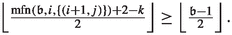This inequality holds if and only if one of the following three cases applies:

  • 

  • is even and .

  • is odd and .

  These assumptions can only hold if $i\in \{1,2\}\vee (i=3\wedge k=0)$. It thus suffices to consider three more cases. For $i=1$, we obtain $\ell ^{\mathfrak {b}+1}(i,j,k)=\left\lceil \frac{\mathfrak {b}+1-1+1-k}{2}\right\rceil =\left\lceil \frac{\mathfrak {b}+1-k}{2}\right\rceil =\phi ^{\sigma }(e).$ Similarly, for $i=2$, we obtain $\ell ^{\mathfrak {b}+1}(i,j,k)=\left\lceil \frac{\mathfrak {b}+1-2+1-k}{2}\right\rceil =\left\lceil \frac{\mathfrak {b}-k}{2}\right\rceil =\left\lfloor \frac{\mathfrak {b}+1-k}{2}\right\rfloor =\phi ^{\sigma }(e).$ Finally, for $i=3$ and $k=0$, we obtain $\ell ^{\mathfrak {b}+1}(i,j,k)=\left\lceil \frac{\mathfrak {b}+1-4+1-k}{2}\right\rceil =\left\lceil \frac{\mathfrak {b}-2-k}{2}\right\rceil =\phi ^{\sigma }(e).$ Hence, for all three cases, choosing the parameter $t_{\mathfrak {b}+1}=0$ yields the desired characterization of $\phi ^{\sigma }(e)$.

• 3. Let $(\mathfrak {b}_i=0\wedge \mathfrak {b}_{i+1}\ne j)$ and $((\mathfrak {b}+1)_i=0\wedge (\mathfrak {b}+1)_{i+1}\ne j)$, implying $i>\nu$. First assume . Then $\ell ^{\mathfrak {b}}(i,j,k)\ge \mathfrak {b}$ by Lemma 7, implying $\phi ^{\sigma _{\mathfrak {b}}}(e)=\left\lfloor \frac{\mathfrak {b}+1-k}{2}\right\rfloor$. Since $\mathfrak {b}$ is odd, $\left\lfloor \frac{\mathfrak {b}+1-1}{2}\right\rfloor <\mathfrak {m}$. Hence, $(d_{i,j,1},F_{i,j})$ was applied during Phase 1 of $\sigma _{\mathfrak {b}}\rightarrow \sigma$ and $e=(d_{i,j,0},F_{i,j})\notin \mathfrak {A}_{\sigma _{\mathfrak {b}}}^{\sigma }$. Thus, since $\ell ^{\mathfrak {b}+1}(i,j,k)\ge \mathfrak {b}+1$ by the choice of i, choosing $t_{\mathfrak {b}+1}=0$ yields the desired characterization.

  Now assume , implying $i<m=\max \{i:\beta ^{\sigma }_i=1\}$. Using $i>\nu \ge 2$, it is easy to verify that this yields $\ell ^{\mathfrak {b}}(i,j,k)\le \left\lfloor \frac{\mathfrak {b}+1-k}{2}\right\rfloor -1$.$^{3}$ If $\sigma _{\mathfrak {b}}(d_{i,j,k})\ne F_{i,j}$, this implies $\phi ^{\sigma _{\mathfrak {b}}}(d_{i,j,k},F_{i,j})\le \ell ^{\mathfrak {b}}(i,j,k)\le \left\lfloor \frac{\mathfrak {b}+1-k}{2}\right\rfloor -1$. Then, by Corollary 1 the switch was applied during Phase 1. We may hence assume $\sigma _{\mathfrak {b}}(d_{i,j,k})=F_{i,j}$, implying that we have $\phi ^{\sigma _{\mathfrak {b}}}(e)=\ell ^{\mathfrak {b}}(i,j,k)+1\le \left\lfloor \frac{\mathfrak {b}+1-k}{2}\right\rfloor$ as well as $\phi ^{\sigma _{\mathfrak {b}}}(e)\le \mathfrak {m}-1$ by Property Or1$_{i,j,k}$. As we assume $e\notin \mathfrak {A}_{\sigma _{\mathfrak {b}}}^{\sigma }$, it suffices to consider the case $\phi ^{\sigma }(e)=\phi ^{\sigma _{\mathfrak {b}}}(e)=\mathfrak {m}-1$ since e is applied during Phase 5 otherwise (see Corollary 12). Since $\ell ^{\mathfrak {b}+1}(i,j,k)=\ell ^{\mathfrak {b}}(i,j,k)+1$ by Lemma 9, choosing $t_{\mathfrak {b}+1}=0$ yields the desired characterization.

• 4. Let $(\mathfrak {b}_i=0\wedge \mathfrak {b}_{i+1}\ne j)$ and $((\mathfrak {b}+1)_i=1\wedge (\mathfrak {b}+1)_{i+1}\ne j)$, i.e., $i=\nu$. The statement follows by the same argument used earlier if . Hence let , implying $\ell ^{\mathfrak {b}}(\nu ,j,k)=\left\lfloor \frac{\mathfrak {b}+1-k}{2}\right\rfloor .$ Since $\sigma _{\mathfrak {b}}$ is a canonical strategy for $\mathfrak {b}$, we have $\sigma _{\mathfrak {b}}(d_{i,j,k})\ne F_{i,j}$. Assume $\phi ^{\sigma _{\mathfrak {b}}}(e)=\ell ^{\mathfrak {b}}(i,j,k)$. Then $\phi ^{\sigma }(e)=\left\lfloor \frac{\mathfrak {b}+1-k}{2}\right\rfloor$ and the same arguments used in the third case can be used to show the statement. Assume $\phi ^{\sigma }(e)=\ell ^{\mathfrak {b}}(i,j,k)-1$. Then $\phi ^{\sigma _{\mathfrak {b}}}(e)=\mathfrak {m}-1$ since we need to have $k=0$ by Property Or3$_{i,j,k}$. But this implies that e was switched during Phase 1 and that we do not need to consider it here.

• 5. Finally, let $(\mathfrak {b}_i=0\wedge \mathfrak {b}_{i+1}=j)$. We only need to consider the case $(\mathfrak {b}+1)_i=0\wedge (\mathfrak {b}+1)_{i+1}=j$, implying $i>\nu$. If , the statement follows by the same arguments made earlier. Otherwise, we can also use the previous same arguments since $\ell ^{\mathfrak {b}}(i,j,k)>\left\lfloor \frac{\mathfrak {b}+1-k}{2}\right\rfloor$ implies $\phi ^{\sigma }(e)=\left\lfloor \frac{\mathfrak {b}+1-k}{2}\right\rfloor$.

It remains to investigate edges $(g_*,F_{*,*})$. We prove that Table 2 specifies their occurrence records by inductively proving the following statement: Let $\sigma _{\mathfrak {b}}\in \varLambda _{\iota }$ be a canonical strategy for $\mathfrak {b}\in \mathcal {B}_n$ calculated by the Strategy Improvement Algorithm. Then $\phi ^{\sigma _{\mathfrak {b}}}(g_i,F_{i,j})\le \min _{k\in \{0,1\}}\phi ^{\sigma _{\mathfrak {b}}}(d_{i,j,k},F_{i,j})$.

For simplicity, we interpret the improving switch $(g_{\nu },F_{\nu ,\mathfrak {b}_{\nu +1}})$ that might technically be applied at the beginning of Phase 2 or 3 as an improving switch that is applied during Phase 1. We prove the statement via induction on $\mathfrak {b}$. We briefly discuss how the statement can be proven for $i\ne 1$ and do not discuss the formal detail or the case $i=1$.$^{3}$ As we consider several earlier strategies during the inductive step, we show that the statement holds for all $\mathfrak {b}\le 2^{i}.$

Thus, let $\mathfrak {b}\le 2^{i}{=}{:}\tilde{\mathfrak {b}}$ and consider some edge $e{:}{=}(g_i,F_{i,j})$. Then $\tilde{\mathfrak {b}}_{i+1}=1$ and $\mathfrak {b}'_{i+1}=0$ for all $\mathfrak {b}'\le \tilde{\mathfrak {b}}$. We prove that e was applied at most once when transitioning from $\iota$ to $\sigma _{\tilde{\mathfrak {b}}}$ and that this application can only happen during $\sigma _{\tilde{\mathfrak {b}}-1}\rightarrow \sigma _{\tilde{\mathfrak {b}}}$. The statement then follows since it is easy to verify that the occurrence records of the cycle edges of $F_{i,j}$ are both at least one.

Since $\iota (g_i)=0$, e cannot have been applied during Phase 1 of any transition encountered during the sequence $\iota \rightarrow \sigma _{\tilde{\mathfrak {b}}}$ as the choice of $\tilde{\mathfrak {b}}$ implies that there is no $\mathfrak {b}'\le \tilde{\mathfrak {b}}$ with $\mathfrak {b}'_i=1\wedge \mathfrak {b}_{i+1}'=1$. It is also easy to show that this implies that it cannot happen that the cycle center $F_{i,j}$ was closed during Phase 1 if $j=1-\mathfrak {b}'_{i+1}$. The switch $(g_i,F_{i,j})$ can thus only have been applied during some Phase 5. However, since $\iota (g_i)=0$ and due to the choice of $\tilde{\mathfrak {b}}$, this can only happen when transitioning from $\sigma _{\tilde{\mathfrak {b}}-1}$ to $\sigma _{\tilde{\mathfrak {b}}}$.

Thus, the statement holds for $\sigma _{\mathfrak {b}}$ with $\mathfrak {b}\le 2^{i}$. Now, assume that it holds for all $\mathfrak {b}'<\mathfrak {b}$ where $\mathfrak {b}>2^{i}$. We prove that the statement also holds for $\sigma _{\mathfrak {b}}$. Fix some edge $e{:}{=}(g_i,F_{i,j})$ and consider the strategy $\sigma _{\mathfrak {b}-1}$. We begin by arguing that several cases do not need to be considered.

First of all, every improving switch is applied at most once per transition. The statement thus follows by the induction hypothesis if $\min _{k\in \{0,1\}}\phi ^{\sigma _{\mathfrak {b}}}(d_{i,j,k},F_{i,j})>\min _{k\in \{0,1\}}\phi ^{\sigma _{\mathfrak {b}-1}}(d_{i,j,k},F_{i,j})$. We thus assume

$$\begin{aligned} \min _{k\in \{0,1\}}\phi ^{\sigma _{\mathfrak {b}}}(d_{i,j,k},F_{i,j}) =\min _{k\in \{0,1\}}\phi ^{\sigma _{\mathfrak {b}-1}}(d_{i,j,k},F_{i,j}). \end{aligned}$$

(3)

Similarly, if e is not applied during $\sigma _{\mathfrak {b}-1}\rightarrow \sigma _{\mathfrak {b}}$, then the statement also follows by the induction hypothesis. We thus assume $e\in \mathfrak {A}_{\sigma _{\mathfrak {b}-1}}^{\sigma _{\mathfrak {b}}}$.

These observations give first structural insights on $\mathfrak {b}-1$ and $\mathfrak {b}$. First, if $\mathfrak {b}_i=1\wedge (\mathfrak {b}-1)_i=1$, then it is not possible to apply e during $\sigma _{\mathfrak {b}-1}\rightarrow \sigma _{\mathfrak {b}}$. Second, if $\mathfrak {b}_i=1\wedge (\mathfrak {b}-1)_i=0$, then $i=\nu (\mathfrak {b})$. By Definition 2 resp. 4, both cycle centers of level $\nu (\mathfrak {b})$ are open for $\sigma _{\mathfrak {b}-1}$. Hence, Corollary 2 implies that $F_{i,j}$ is closed during $\sigma _{\mathfrak {b}-1}\rightarrow \sigma _{\mathfrak {b}}$ by applying both switches $(d_{i,j,0},F_{i,j})$ and $(d_{i,j,1},F_{i,j})$. But then, Eq. (3) is not fulfilled and the statement follows. This implies that it suffices to consider the case $\mathfrak {b}_i=0$.

It can then be show that these assumptions imply that the occurrence record of the edges $(d_{i,j,*},F_{i,j})$ is “large”.$^{3}$ To be precise, that Eq. (3), $e\in \mathfrak {A}_{\sigma _{\mathfrak {b}-1}}^{\sigma _{\mathfrak {b}}}$ and $\mathfrak {b}_i=0$ imply

$$\begin{aligned} \min _{k\in \{0,1\}}\phi ^{\sigma _{\mathfrak {b}-1}}(d_{i,j,k},F_{i,j})\ge \left\lfloor \frac{\mathfrak {b}}{2}\right\rfloor -1. \end{aligned}$$

(4)

It then suffices to prove $\phi ^{\sigma _{\mathfrak {b}-1}}(g_i,F_{i,j})<\left\lfloor \frac{\mathfrak {b}}{2}\right\rfloor -1$ to complete the proof.

We begin by proving that we cannot have $(\mathfrak {b}-1)_i=1$. Let, for the sake of contradiction, $(\mathfrak {b}-1)_i=1$. Then, as $\mathfrak {b}_i=0$, we have $i<\nu (\mathfrak {b})$ and consequently $(\mathfrak {b}-1)_{i+1}\ne \mathfrak {b}_{i+1}$. It further implies that $\mathfrak {b}$ is even. Then, since $e\in \mathfrak {A}_{\sigma _{\mathfrak {b}-1}}^{\sigma _{\mathfrak {b}}}$ by assumption, it was applied during Phase 5 of $\sigma _{\mathfrak {b}-1}\rightarrow \sigma _{\mathfrak {b}}$. This implies $j=0$ in $S_n$ resp. $j=\mathfrak {b}_{i+1}=1-(\mathfrak {b}-1)_{i+1}$ in $M_n$. Consider $M_n$ first. Then, since $(\mathfrak {b}-1)_i=1\wedge j=1-(\mathfrak {b}-1)_{i+1}$ imply $\ell ^{\mathfrak {b}-1}(i,j,k)\ge \left\lfloor \frac{\mathfrak {b}-k}{2}\right\rfloor +1$ by Lemma 7, we obtain $\phi ^{\sigma _{\mathfrak {b}-1}}(d_{i,j,k},F_{i,j})=\left\lfloor \frac{\mathfrak {b}-k}{2}\right\rfloor$.

In addition, since $\phi ^{\sigma _{\mathfrak {b}-1}}(d_{i,j,k},F_{i,j})\ne \ell ^{\mathfrak {b}-1}(i,j,k)+1$ for both $k\in \{0,1\}$, $F_{i,j}$ is then open with respect to $\sigma _{\mathfrak {b}-1}$ by Property Or2$_{i,j,*}$. This implies that $(d_{i,j,1},F_{i,1})$ is applied during Phase 1 of $\sigma _{\mathfrak {b}-1}\rightarrow \sigma _{\mathfrak {b}}$. But then $\min _{k\in \{0,1\}}\phi ^{\sigma _{\mathfrak {b}-1}}(d_{i,j,k},F_{i,j})<\min _{k\in \{0,1\}}\phi ^{\sigma _{\mathfrak {b}}}(d_{i,j,k},F_{i,j}),$ contradicting our assumption. Now consider the case $G_n=S_n$. If $j=0=1-(\mathfrak {b}-1)_{i+1}$, then the statement follows by the same arguments. This is the case if and only if $i<\nu (\mathfrak {b})-1$, so let $i=\nu (\mathfrak {b})-1$. By Definition 2, this implies $\sigma _{\mathfrak {b}-1}(g_i)=F_{i,0}$. Since $F_{i,0}$ is then closed during Phase 1 of the transition $\sigma _{\mathfrak {b}-1}\rightarrow \sigma _{\mathfrak {b}}$ and since $(g_i,F_{i,1})$ cannot be applied during Phase 5 if $G_n=S_n$, this is a contradiction.

It thus suffices to consider the case $(\mathfrak {b}-1)_i=0$. To simplify notation, we denote the binary number obtained by subtracting 1 from a binary number $(\mathfrak {b}'_n,\dots ,\mathfrak {b}'_1)$ by $[\mathfrak {b}'_{n},\dots ,\mathfrak {b}'_{1}]-1$. Then, $\mathfrak {b}$ and $\mathfrak {b}-1$ can be represented as

$$\begin{aligned} \mathfrak {b}&=(\mathfrak {b}_n,\dots ,\mathfrak {b}_{i+1},\varvec{0},\mathfrak {b}_{i-1},\dots ,\mathfrak {b}_1), \\ \mathfrak {b}-1&=(\mathfrak {b}_n,\dots ,\mathfrak {b}_{i+1},\varvec{0},[\mathfrak {b}_{i-1},\dots ,\mathfrak {b}_1]-1) \end{aligned}$$

where bit i is marked in bold. The idea of the proof is now the following. We define two smaller numbers that are relevant for the application of $(g_i,F_{i,j})$. We use these numbers and the induction hypothesis to prove that even if $(g_i,F_{i,j})$ was applied during (nearly) all of these transitions, the bound that we claim still holds.

We thus define $\bar{\mathfrak {b}}=([\mathfrak {b}_n,\dots ,\mathfrak {b}_{i+1}]-1,\varvec{1},1\dots ,1)$ and $\tilde{\mathfrak {b}}=([\mathfrak {b}_n,\dots ,\mathfrak {b}_{i+1}]-1,\varvec{1},0,\dots ,0)$ where bit i is again marked in bold. Note that these numbers are well-defined since $\mathfrak {b}\ge 2^{i}$.

Consider $\tilde{\mathfrak {b}}$. Let $\mathfrak {N}(\tilde{\mathfrak {b}}, \mathfrak {b}-1)$ denote the number of applications of $(g_i,F_{i,j})$ when transitioning from $\sigma _{\tilde{\mathfrak {b}}}$ to $\sigma _{\mathfrak {b}-1}$. Then, since $\mathfrak {b}'_i=1$ for all $\mathfrak {b}'\in \{\tilde{\mathfrak {b}},\dots ,\bar{\mathfrak {b}}\}$, we have $\mathfrak {N}(\tilde{\mathfrak {b}},\mathfrak {b}-1)=\mathfrak {N}(\bar{\mathfrak {b}}, \mathfrak {b}-1)$. We thus can describe the occurrence record of $(g_i,F_{i,j})$ as

$$\begin{aligned} \phi ^{\sigma _{\mathfrak {b}-1}}(g_i,F_{i,j})= & {} \mathfrak {N}(0,\mathfrak {b}-1)=\mathfrak {N}(0,\tilde{\mathfrak {b}})+\mathfrak {N}(\tilde{\mathfrak {b}},\mathfrak {b}-1)\\= & {} \phi ^{\sigma _{\tilde{\mathfrak {b}}}}(g_i,F_{i,j})+\mathfrak {N}(\bar{\mathfrak {b}},\mathfrak {b}-1). \end{aligned}$$

Our goal is to bound the two terms on the right-hand side. Due to the induction hypothesis, the first term can be bounded by $\lfloor \frac{\tilde{\mathfrak {b}}}{2}\rfloor$. Since every improving switch is applied at most once per transition by Corollary 13, we have $\mathfrak {N}(\bar{\mathfrak {b}},\mathfrak {b}-1)\le (\mathfrak {b}-1)-\bar{\mathfrak {b}}$. However, this upper bound is not strong enough. It can however be proven that $(g_i,F_{i,j})$ was not applied during all transition from $\bar{\mathfrak {b}}$ to $\mathfrak {b}-1$. More precisely, $\mathfrak {N}(\bar{\mathfrak {b}},\mathfrak {b}-1)\le (\mathfrak {b}-1)-\bar{\mathfrak {b}}-1$. Combining these results and using $\bar{\mathfrak {b}}=\mathfrak {b}-\sum (\mathfrak {b},i)-1$ and $\tilde{\mathfrak {b}}=\mathfrak {b}-\sum (\mathfrak {b},i)-2^{i-1}$ yields the statement.$^{3}$

We can now combine the previous arguments to prove Lemma 5. Note that this implies Lemma 6.

Lemma 5 Let $\sigma _{\mathfrak {b}}\in \varLambda _{\iota }$ be a canonical strategy for $\mathfrak {b}$ fulfilling the canonical conditions. Let $\sigma \in \varLambda _{\sigma _{\mathfrak {b}}}$ be a strategy obtained by applying a sequence of improving switches to $\sigma _{\mathfrak {b}}$. Let $\sigma$ have the properties of row k of Table 6and let $I_{\sigma }$ be described by row k of Table 7for some $k\in \{1,\dots ,5\}$. Then, applying improving switches according to Zadeh’s pivot rule and our tie-breaking rule produces a strategy $\sigma '$ that is described by the next feasible rows of Tables 6and 7.

Proof

By Lemmas 7, 8, 9 and 10, it suffices to consider the case $k=5$. By Lemma 11, applying improving switches to a canonical strategy $\sigma _{\mathfrak {b}}$ for $\mathfrak {b}$ produces a canonical strategy $\sigma _{\mathfrak {b}+1}$ for $\mathfrak {b}+1$. It suffices to prove that $\sigma _{\mathfrak {b}+1}$ fulfills the canonical conditions.

By Corollary 13, Table 2 correctly specifies the occurrence record of all edges when interpreted for $\mathfrak {b}+1$. By Lemma 12, $\sigma _{\mathfrak {b}+1}$ has Properties (Or1)$_{*,*,*}$ to (Or4)$_{*,*,*}$. By Corollary 13, each improving switch was applied at most once when transitioning from $\sigma _{\mathfrak {b}}\rightarrow \sigma _{\mathfrak {b}+1}$. Consequently, $\sigma _{\mathfrak {b}+1}$ fulfills the canonical conditions. $\square$

This now enables us to prove our final theorem.

Theorem 4 Applying the Strategy Improvement Algorithm with Zadeh’s pivot rule and the strategy-based tie-breaking rule described in Definition 7on the game $G_n$ of size O(n) needs at least $2^n$ iterations when using $\iota$ as the initial player 0 strategy.

Proof

This follows by Lemma 4 and by applying Lemma 6 iteratively. $\square$

References

Avis, D., Chvátal, V.: Notes on Bland’s pivoting rule. In: Polyhedral Combinatorics: Dedicated to the memory of D.R. Fulkerson, pp. 24–34. Springer, Heidelberg (1978)
Avis, D., Friedmann, O.: An exponential lower bound for Cunningham’s rule. Math. Program. 161(1), 271–305 (2017)
Bertsimas, D., Vempala, S.: Solving convex programs by random walks. J. of the ACM 51(4), 540–556 (2004)
Cunningham, W.H.: Theoretical properties of the network simplex method. Math. of Oper. Res. 4(2), 196–208 (1979)
Dantzig, G.B.: Linear Programming and Extensions. Princeton University Press (1963)
Disser, Y., Friedmann, O., Hopp, A.V.: An Exponential Lower Bound for Zadeh’s pivot rule (2020). Full version. Available at https://arxiv.org/pdf/1911.01074.pdf
Disser, Y., Hopp, A.V.: On Friedmann’s subexponential lower bound for Zadeh’s pivot rule. In: Proceedings of the 20th Conference on Integer Programming and Combinatorial Optimization (IPCO) pp. 168–180 (2019)
Disser, Y., Skutella, M.: The simplex algorithm is NP-mighty. ACM Trans. on Algorithms 15(1), 5–19 (2018)
Dunagan, J., Vempala, S.: A simple polynomial-time rescaling algorithm for solving linear programs. Math. Program. 114(1), 101–114 (2007)
Fearnley, J.: Exponential lower bounds for policy iteration. In: Proceedings of the 37th International Colloquium on Automata, Languages, and Programming (ICALP) pp. 551–562 (2010)
Fearnley, J., Savani, R.: The complexity of the simplex method. In: Proceedings of the 47th Annual ACM on Symposium on Theory of Computing (STOC) pp. 201–208 (2015)
Friedmann, O.: An exponential lower bound for the parity game strategy improvement algorithm as we know it. In: Proceedings of the 24th Annual IEEE Symposium on Logic In Computer Science (LICS) pp. 145–156 (2009)
Friedmann, O.: An exponential lower bound for the latest deterministic strategy iteration algorithms. Logical Methods in Computer Sci. 7(3:19), 1–42 (2011)
Friedmann, O.: Exponential Lower Bounds for Solving Infinitary Payoff Games and Linear Programs. PhD thesis, University of Munich (2011)
Friedmann, O.: A subexponential lower bound for Zadeh’s pivoting rule for solving linear programs and games. In: Proceedings of the 15th International Conference on Integer Programming and Combinatoral Optimization (IPCO) pp. 192–206 (2011)
Friedmann, O., Hansen, T.D., Zwick, U.: A subexponential lower bound for the random facet algorithm for parity games. In: Proceedings of the 22nd Annual ACM-SIAM Symposium on Discrete Algorithms (SODA) pp. 202–216 (2011)
Friedmann, O., Hansen, T.D., Zwick, U.: Subexponential lower bounds for randomized pivoting rules for the simplex algorithm. In: Proceedings of the 43rd Annual ACM Symposium on Theory of Computing (STOC) pp. 283–292 (2011)
Friedmann, O., Hansen, T.D., Zwick, U.: Errata for: A subexponential lower bound for the random facet algorithm for parity games (2014). CoRR, abs/1410.7871
Friedmann, O., Lange, M.: PGSolver, version 4.1 (June 2017). Available at https://github.com/tcsprojects/pgsolver
Goldfarb, D., Sit, W.Y.: Worst case behavior of the steepest edge simplex method. Discrete Applied Math. 1(4), 277–285 (1979)
Hansen, T.D.: Worst-case Analysis of Strategy Iteration and the Simplex Method. PhD thesis, Department Office Computer Science, Aarhus University (2012)
Hansen, T.D., Zwick, U.: An improved version of the random-facet pivoting rule for the simplex algorithm. In: Proceedings of the 47th Annual ACM on Symposium on Theory of Computing (STOC) pp. 209–218 (2015)
Howard, R.A.: Dynamic Programming and Markov Processes. MIT Press (1960)
Animation of the counter for 3 and 4 levels (2019). https://oliverfriedmann.com/downloads/add/zadeh-exponential-animation-3.pdfhttps://oliverfriedmann.com/downloads/add/zadeh-exponential-animation-4.pdf
Kalai, G.: A subexponential randomized simplex algorithm. In: Proceedings of the 24th Annual ACM Symposium on Theory of Computing (STOC) pp. 475–482 (1992)
Kalai, G.: Linear programming, the simplex algorithm and simple polytopes. Math. Program. 79, 217–233 (1997)
Karmarkar, N.: A new polynomial-time algorithm for linear programming. In: Proceedings of the 16th Annual ACM Symposium on Theory of Computing (STOC), pp. 302–311 (1984)
Kelner, J.A., Spielman, D.A.: A randomized polynomial-time simplex algorithm for linear programming. In: Proceedings of the 38th Annual ACM Symposium on Theory of Computing (STOC) pp. 51–60 (2006)
Khachiyan, L.G.: Polynomial algorithms in linear programming. USSR Comput. Math. and Math. Phys. 20(1), 53–72 (1980)
Klee, V., Minty, G.J.: How good is the simplex algorithm? In: Inequalities III, pp. 159–175. Academic Press, New York (1972)
Küsters, R.: Memoryless determinacy of parity games. In: Grädel, Erich, Thomas, Wolfgang, Wilke, Thomas (eds.) Automata Logics, and Infinite Games. Springer, Berlin Heidelberg (2002)
Matoušek, J., Sharir, M., Welzl, E.: A subexponential bound for linear programming. Algorithmica 16(4–5), 498–516 (1996)
Matoušek, J., Szabó, T.: Random edge can be exponential on abstract cubes. Adv. in Math. 204(1), 262–277 (2006)
Puterman, M.L.: Markov Decision Processes: Discrete Stochastic Dynamic Programming. John Wiley & Sons Inc, New York (2005)
Santos, F.: A counterexample to the Hirsch conjecture. Annals of Math. 176(1), 383–412 (2012)
Smale, S.: Mathematical problems for the next century. The Math. Intell. 20(2), 7–15 (1998)
Solms, Felix: Implementing a sink game solver. Master’s thesis, TU Darmstadt (2021). implementation available at https://www2.mathematik.tu-darmstadt.de/~disser/data/VisualSinkGameSolver.zip
Szpilrajn, E.: Sur l’extension de l’ordre partiel. Fundamenta Math. 16, 386–389 (1930)
Thomas, A.: Exponential lower bounds for history-based simplex pivot rules on abstract cubes. In: Proceedings of the 25th Annual European Symposium on Algorithms (ESA) pp. 69(14) (2017)
Tijms, H.C.: A First Course in Stochastic Models. John Wiley & Sons, Ltd (2004)
Todd, M.J.: An improved Kalai-Kleitman bound for the diameter of a polyhedron. SIAM J. on Discrete Math. 28(4), 1944–1947 (2014)
Vöge, J., Jurdziński, M.: A discrete strategy improvement algorithm for solving parity games. In: Computer Aided Verification, pp. 202–215 (2000)
Zadeh, N.: What is the worst case behavior of the simplex algorithm? Technical Report 27. Departments of Operations Research, Stanford (1980)
Acknowledgements
We would like to thank Felix Solms for his implementation of a sink game solver [37], which helped us to iron out quantitative details of our construction.
Funding
Open Access funding enabled and organized by Projekt DEAL.
Author information
Authors and Affiliations
Corresponding author
Additional information
Publisher's Note
Springer Nature remains neutral with regard to jurisdictional claims in published maps and institutional affiliations.
The work of Yann Disser and Alexander V. Hopp was supported by the ‘Excellence Initiative’ of the German Federal and State Governments and the Graduate School CE at TU Darmstadt. Alexander V. Hopp’s work was mainly contributed during his time at the Department of Mathematics at the TU Darmstadt.