
Abstract
Nuclear power has the potential to provide significant amounts of reliable electricity generation without carbon dioxide emissions. Disposing of radioactive waste is, however, an ongoing challenge, and if it is to be buried, the characterisation of the regional groundwater system is vital to protect the anthroposphere. This aspect is understudied in comparison to the engineered facility; yet, selecting a suitable groundwater setting can ensure radionuclide isolation hundreds of thousands of years beyond that provided by the engineered structure. This paper presents a multi-faceted scoping tool to quantitatively assess, and directly compare, the regional hydrogeological prospectivity of different groundwater settings for disposal at an early stage of the site selection process. The scoping tool is demonstrated using geological data from three distinct UK groundwater settings as a case study. Results indicate a significant difference in the performance potential of different regional groundwater settings to ensure long-term waste containment.
Résumé
L’énergie nucléaire offre la possibilité de fournir des quantités importantes d’électricité fiable sans émettre de gaz carbonique. L’entreposage des déchets radioactifs est cependant un défi permanent et, s’agissant de leur enfouissement, la caractérisation du système hydrogéologique régional est essentielle pour la protection de l’anthroposphère. Cet aspect est sous-étudié par rapport à ce qui est réalisé pour la conception des sites d’entreposage, pourtant la sélection d’un contexte hydrogéologique approprié peut assurer l’isolement des radionucléides sur des centaines de milliers d’années au-delà de celle assurée par la structure d’ingénierie. Cet article présente un outil de ciblage multi-facettes pour évaluer quantitativement et comparer directement, les potentialités hydrogéologiques régionales de différents contextes hydrogéologiques pour l’entreposage à un stade précoce du processus de sélection de site. L’outil de ciblage est présenté en utilisant les données géologiques de trois contextes hydrogéologiques distincts du Royaume-Uni comme cas d’étude. Les résultats indiquent une différence significative du potentiel de performance des différents contextes hydrogéologiques régionaux permettant d’assurer le confinement des déchets sur le long-terme.
Resumen
La energía nuclear tiene el potencial de proporcionar cantidades significativas de generación de electricidad segura sin emisiones de dióxido de carbono. Sin embargo, la eliminación de los residuos radiactivos es un desafío permanente, y si se va a enterrar, la caracterización del sistema regional de aguas subterráneas es vital para proteger la antroposfera. Este aspecto está poco estudiado en comparación con las instalaciones de ingeniería, sin embargo, la selección de un ambiente adecuado de aguas subterráneas puede asegurar el aislamiento de los radionúclidos cientos de miles de años más allá de lo que proporciona la estructura de ingeniería. En este documento se presenta un instrumento polifacético de determinación del alcance para evaluar cuantitativamente y comparar directamente la prospectividad hidrogeológica regional de diferentes entornos de aguas subterráneas para su eliminación en una etapa temprana del proceso de selección del emplazamiento. La herramienta de determinación del alcance se demuestra utilizando como estudio de caso datos geológicos de tres ámbitos distintos de aguas subterráneas del Reino Unido. Los resultados indican una diferencia significativa en el potencial de rendimiento de los diferentes ámbitos regionales de aguas subterráneas para garantizar la contención de los desechos a largo plazo.
摘要
核电有潜力提供大量可靠的发电而且不会排放二氧化碳。但是,放射性废物的处置一直是一个挑战,如果要掩埋,区域地下水系统的特征对于保护人类圈至关重要。与工程设施相比,这方面的研究不足,但是,选择合适的地下水条件可以确保放射性核素隔离度比工程结构所提供的要高数十万年。本文提出了一个多方面范围界定的工具,可以定量评估和直接比较不同地下水条件的区域水文地质前景,以便在选址过程的早期阶段进行处理。作为案例研究,采用了英国三个不同地下水条件的地质数据展示了范围界定工具。结果表明,不同区域地下水条件的性能潜力在确保长期废物污染方面存在显着差异。
Resumo
A energia nuclear tem o potencial de fornecer quantidades significativas de geração confiável de eletricidade sem emissão de dióxido de carbono. O descarte de resíduos radioativos é, no entanto, um desafio contínuo e, para ser enterrado, a caracterização do sistema regional de águas subterrâneas é vital para proteger a antroposfera. Esse aspecto é pouco estudado em comparação com a instalação de engenharia, no entanto, a seleção de uma configuração adequada de água subterrânea pode garantir o isolamento de radionuclídeos centenas de milhares de anos além do fornecido pela estrutura de engenharia. Este artigo apresenta uma ferramenta de escopo multifacetada para avaliar quantitativamente, e comparar diretamente a prospectiva hidrogeológica regional de diferentes configurações de águas subterrâneas para o processo de seleção do local de descarte em um estágio inicial. A ferramenta de escopo é demonstrada usando dados geológicos de três configurações distintas de água subterrânea do Reino Unido como um estudo de caso. Os resultados indicam uma diferença significativa no potencial de desempenho de diferentes configurações regionais de águas subterrâneas para garantir a contenção de resíduos a longo prazo.
Introduction
Nuclear power provides a reliable and low carbon source of electrical energy, currently accounting for 21% of the total UK electricity production (BEIS 2017). An unfortunate by-product of this process is the generation of highly radioactive and chemical-toxic waste (NDA 2017), which must be managed safely. By 2125 the UK is predicted to have 4.77 million m3 of packaged radioactive waste requiring management (NDA 2017). The chosen international approach is to dispose of the most radioactive of this waste (approx. 650,000 m3 in the UK (NDA 2014)) within a deep geological disposal facility (GDF) situated 200–1,000 m below the ground surface (Apted and Ahn 2017; NDA 2013, 2014; Streffer et al. 2011). Sweden and Finland are the only countries to have officially selected disposal locations for their higher activity civil waste legacy. The Waste Isolation Pilot Plant in the USA is accepting military-derived radioactive waste. All other waste producing nations (including the UK) remain in the search phase.
Geological disposal facilities must be designed as a series of complimentary yet independent physical and chemical barriers (IAEA 2009, 2011a). These barriers are intended to contain and isolate the waste within the subsurface for many hundreds of thousands to millions of years (Environment Agency 2009; IAEA 2011a; RWM 2016a). Typical repository safety assessments are undertaken over a 1 million-year timeframe (Metcalfe et al. 2008), with the risk of death regulated at less than one-in-a-million per annum (Environment Agency 2009).
The engineered barriers will lose their integrity over timescales of tens to hundreds of thousands of years (RWM 2016a) due to chemical and mechanical degradation (Corkhill et al. 2013; Gin 2014; King et al. 2016; Metcalfe et al. 2008; RWM 2016a; Sharland et al. 2008), after which the natural barrier will become the main operational barrier (RWM 2016a). Although independent natural barrier assessment is vital to ensure overall repository performance (RWM 2016b), very little research has followed this approach. This is likely due to the geospatial and temporal complexity of subsurface characterisation.
The natural barrier comprises the rock mass and groundwater surrounding the engineered facility. Groundwater movement is an important component of a disposal facility as it is a primary transport mechanism through which released waste will be returned to the surface (RWM 2016b). It also controls the degradation rate of the engineered system (Corkhill et al. 2013; Gin 2014; NDA 2010a; RWM 2016a).
The protection of UK groundwater resources is driven by the European Union’s Groundwater Directive (2006/118/EEC) which states that the release of hazardous substances to groundwater should be prevented, and nonhazardous substances minimised. The approach to groundwater protection from developments and activities, e.g. infrastructure, landfills and liquid effluent discharges, is set out in domestic legislation, e.g. Environment Agency (2018).
The risk to groundwater is assessed through structured risk assessments. Within the UK, developments or activities deemed to pose a risk to groundwater are generally disallowed within 50 days (source protection zone 1; SPZ1) or 400 days (SPZ2) travel time to a potentially significant receptor, e.g. a potable well. Furthermore, developments or activities are tightly regulated within the same groundwater catchment (SPZ3), including when separated by a protective geological cover (Environment Agency 2018). Long groundwater pathway lengths (from source to receptor), slow groundwater velocities, and low-permeability geological barrier are all therefore important characteristics for groundwater protection.
Where disposal or storage of potential pollutants beneath the water table is concerned, e.g. some landfills, both engineered barriers and a low permeability geological barrier are required. Common engineered barriers for landfills include low permeability clay or geosynthetic liners (<1E-09 m/s, Landfill Directive, 1999/31/EC), and leachate extraction to ensure hydraulic containment.
Argillaceous (including clay), evaporitic and crystalline rocks have all been identified as potentially suitable low-permeability GDF host rocks (NDA 2014). Research has found that within these types of formations, the groundwater flow rate can be low enough that diffusion dominates contaminant transport mechanisms (Colley and Thompson 1991; Falck and Hooker 1990; Miller et al. 1994; Wollenberg and Flexser 1984). Under these conditions, and in combination with strong sorption properties—argillaceous rocks and to a lesser extent crystalline rocks (Berry et al. 1999; NDA 2010b)—migrating radionuclides can move extraordinarily slowly. For example, a naturally occurring uranium ore surrounded by a clay rich halo (Cigar Lake, Canada) indicates containment of uranium elements in the near field for circa. 1.3 billion years (NDA 2010c). Because of the slow flow rates and strong sorption potential, clays have been the focus of host rock investigations in both France (ANDRA 2005) and Switzerland (Nagra 2002).
Although hydraulic containment can be ensured over the short-term using groundwater extraction techniques (like for near-surface landfills), long-term containment relies more heavily on passive measures (Streffer et al. 2011). A setting must therefore be selected in which pollutants are transported naturally away from resources, not towards them. This requires consideration of the regional groundwater system.
For clarification, this research considers groundwater as a pathway, and not a receptor. To ensure protection of potentially significant resources, e.g. aquifers or mineral seams (RWM 2016b), the groundwater pathway should exhibit certain ‘protective’ physical and chemical characteristics. Hydrogeological characteristics (HCs) identified by Chapman et al. 1986 as being of benefit for radioactive waste containment include: HC.1, slow regional groundwater movement; HC.2, long groundwater pathways prior to surface discharge; HC.3, groundwater progressively mixing with older deeper waters; HC.4, slow local groundwater movement; and HC.5, predictable groundwater pathways despite parameter and process uncertainties (Chapman et al. 1986). Separation of near-surface from deeper groundwater systems (HC.6) has also been listed as a beneficial hydrogeological characteristic (RWM 2016b).
These characteristics are exemplified through a series of idealised regional hydrogeological regimes (HRs) which include: inland basin, modified basin limb, seaward-dipping and offshore sediments, basement rocks under sedimentary cover, hard rocks in low-relief coastal environments, and small islands (Chapman et al. 1986; Fig. 1).

Conceptual illustration of idealised regional hydrogeological regimes which exhibit wide ranging groundwater characteristics considered to be of benefit for long-term radioactive waste containment. Image digitised and adapted from Chapman et al. (1986) with categorization as: a inland basin, a′ modified basin limb, b seaward-dipping and offshore sediments, c basement rocks under sedimentary cover, d hard rocks in low-relief coastal environments, and e small islands
The HCs are controlled by regional geographical and geological features such as mountain chains, river basins and geological formations (Tóth 1963). The natural barrier should thus be assessed with respect to the regional setting, covering areas of tens of kilometres.
Consideration of the quality of the natural barrier and regional setting has been of variable importance within international site selection processes—for example, Forsmark (Sweden) was selected over Laxmar (both situated in low relief tectonic lenses of the Ferroscandianivian shield) due to natural barrier features which promote ‘better prospects for achieving long term safety’, including: ‘fewer water-conducing fractures’ and ‘limited groundwater flow through repository’ (SKB 2009). In contrast, the shortlisting and selection of Sellafield (UK) for an underground rock characterisation facility (RCF) (commonly perceived as a precursor to a GDF) (Letter from the Director of Infrastructure & Planning for the North West, dated 17 March 1997; UK Parliament 1997) was ‘strongly influenced by non-technical [social, political and economic] factors’ such as ‘restricted to sites that were owned by central government, or by its nuclear industry shareholder’ (Nirex 2005a) and because ‘waste transport would be less of an issue’ (Nirex 2002, 2005a). The planning application for the RCF at Sellafield was refused in 1997 due, in part, to the site being ‘geologically and hydrogeologically much less simple and more complex than would be expected of a choice based principally on scientific and technical grounds’ (Letter from the director of Infrastructure & Planning for the North West, dated 17th March 1997; UK Parliament 1997). Lack of focus on the natural barrier characteristics was thus a contributing factor to the rejected application for the RCF.
Although demonstration of the natural barrier performance is a prerequisite for the safety assessment (IAEA 2011a), no obligatory method exists which makes comparison of the relative benefits of different regional settings difficult. This paper provides a solution to this challenge by proposing a method, based on the set of established and transferable groundwater characteristics defined by Chapman et al. 1986, to compare the prospective performance of different settings. Three coupled process models are developed based on UK data as a case study. Variable rock permeability scenarios are explored as key performance uncertainties (Domenico and Schwartz 1997). Settings are compared to an ‘idealised’ benchmark scenario. Results indicate that the natural barrier, and thus overall repository performance, varies up to a factor of 4 between assessed settings.
Methods
The method is undertaken in three stages: firstly, a benchmark scenario is defined against which the HCs of the chosen settings could be directly compared; secondly, three settings are selected for assessment; and thirdly, numerical regional groundwater flow models to represent each of the selected settings are developed.
The benchmark scenario
The benchmark scenario is defined based on the previously listed beneficial HCs from Chapman et al. 1986, which is aligned with a common resource protection strategy as discussed previously. The HCs are converted into quantifiable parameters (Ps), such that P.1 quantitatively represents HC.1, etc. The Ps have been developed so as to be applicable to any modelled setting The conditions chosen for P.1–P.4 (summarised in the following) are detailed further in Table S1 of the electronic supplementary material (ESM), illustrated in Fig. S4 of the ESM and justified in section ‘Implementation of the proposed method’
-
P.1. (representing HC.1) is the percentage of the far-field domain (20 km in length by 2 km depth area) with very slow advective velocity.
-
P.2. (representing HC.2) is the total length of the groundwater pathway from repository top to model discharge/exit point.
-
P.3. (representing HC.3) is the depth of the groundwater pathway discharge/exit point relative to the top of the repository.
-
P.4. (representing HC.4) is the distance released radionuclides travel over the first 10,000 years.
As shown in the preceding, HC.1–HC.4 have been integrated directly into the assessment criteria. HC.5 is accounted for by running two versions of each modelled setting —a most-likely permeability and a high permeability model—in order to account for key epistemic uncertainties. The difference in overall scores, therefore, reflects the predictability of each setting as a result of permeability uncertainty. Finally, HC.6 is already accounted for through HC.1–HC.4 as a coupled near surface to deep groundwater system would permit direct return of radionuclides to the surface (short and ascending groundwater pathways) and would be subject to faster groundwater velocities through connection to topographic drive. The findings of HC.6 are therefore discussed qualitatively for each modelled site. The benchmark scenario scores 0, with points accrued (up to 20) for negative characteristics (Fig. 2).

a Idealised benchmark outflow scenario, including hydrogeological parameters 1–4, against which all model scenarios are assessed. b Proposed bar-chart assessment criteria to be applied to all model scenarios in which a score of 0 indicates beneficial hydrogeological characteristics for long-term waste containment, and a score of 20 indicates poor groundwater characteristics
Site selection for assessment
To illustrate this method, three exemplar settings are selected (see Fig. 3). Site selection is based on perceived geological (and therefore hydrogeological) diversity, and historic literature indications of potential hydrogeological suitability as discussed in the following. The UK is used as a case study due to the availability of geological and hydrogeological data. This method could however be applied anywhere in the world as the assessment method is based on universal hydrogeological parameters. At the time of writing, no sites have been officially selected for GDF investigation within the UK.

Location map of chosen UK exemplar case study settings, along with simplified representations of their expected intrinsic permeabilities. Note: discrete fractures are not explicitly represented within this image
Setting 1 will be based on rock geometry and properties from Sellafield (West Cumbria), where £400 million of drilling investigations were undertaken up to 1997 for the purpose of the RCF (Nirex 1997a, b, c, d). Comparison of the HCs of this location to other UK settings is thus anticipated to be of interest to the wider scientific community. The setting also provides an opportunity for model verification from the datasets obtained during the RCF investigations (Nirex 1997a, b, c, d), and from previous site-specific modelling (Fraser-Harris et al. 2015).
Setting 2 is located offshore and is based on rock geometries and properties from the Tynwald Basin (East Irish Sea Basin). Setting 2 was chosen due to laterally extensive low permeability sediments (Jackson et al. 1995, 1997), and a possible offshore dense brine formation (Barnes et al. 2005), indicative of a hydrogeologically stable environment over inter-glacial timescales (Park et al. 2009). This type of setting could be considered potentially analogous to the seaward dipping and offshore sediments type HR (HRs listed in section ‘Introduction’). At the time of writing, no country has disposed of its higher activity waste legacy offshore. Setting 2 is therefore also anticipated to be of wider scientific interest.
Setting 3 beneath Thetford (East Anglia), was chosen due to a laterally extensive sedimentary sequence overlying crystalline basement (Lee et al. 2015), which could be considered analogous to the basement rock beneath sedimentary sequence type HR. This setting therefore has the potential to exhibit advantageous HCs for long-term radioactive waste containment as defined by Chapman et al. 1986.
Model development
This section details the construction of numerical models to represent each of the three chosen settings.
Geometry
Model geometries (approx. 30 km length by 2–4 km depth) were obtained from publicly available 2D British Geological Survey geological cross-sections, and converted into 2D conceptual hydrogeological cross-sections by combining geological units considered to behave in a similar hydrogeological manner. Setting 1 was constructed using a combination of geological cross-sections from Gosforth (BGS 1999a), the lake district fells (Michie 1996) and the previously investigated RCF—Nirex 1997a, b; Fig. S1 of the electronic supplementary material (ESM). Setting 2 was constructed using a geological cross-section from Bootle (BGS 1997), supplemented by offshore borehole and seismic-derived stratigraphic data (Akhurst et al. 1997; Barnes et al. 2005; Jackson et al. 1987; Schlumberger 2016) (Fig. S2 of the ESM). Setting 3 was constructed using a geological cross-section from Swaffham (BGS 1999b), supplemented with additional stratigraphic information for East Anglia (Lee et al. 2015; Fig. S3 of the ESM). Fault zones were represented as 50-m-wide continuum porous media in keeping with previous hydrogeological modelling assessments (Fraser-Harris et al. 2015; McKeown et al. 1999; Nirex 1997c).
Mesh
Two-dimensional (2D) conceptual hydrogeological cross-section geometries were converted into a mesh of 2D triangular elements using the GMSH meshing software (Geuzaine and Remacle 2009). Element sizes ranged from 5 to 100 m, with higher mesh densities applied to thinner hydrogeological units. Setting 1 comprised 173,527 elements, setting 2 comprised 258,920 elements, and setting 3 comprised 117,461 elements.
Material properties
Models were populated with the material properties of porosity, permeability (both ‘most-likely’ and ‘high’ values as a key performance uncertainty), mass dispersion, heat dispersion, storativity, bulk density, thermal capacity, thermal conductivity, specific heat capacity, and specific heat conductivity (Tables S2–S4 of the ESM).
Material properties were applied to each individual hydrogeological unit using site-specific information where available, else generic data ranges were applied. When a lithologically layered hydrogeological unit was present, e.g. for setting 3, the effective horizontal (Kx) and vertical (Kz) permeabilities (m s−1) were calculated using Eqs. (1) and (2) respectively (Lee and Fetter 1994) where k is the hydraulic conductivity (m s−1), n is the number of layers within the aquifer, i is the layer, and b is the layer thickness (m).
Hydraulic conductivities (m s−1) were converted into intrinsic permeability (m2) using Eq. (3) (Domenico and Schwartz 1997). K itself comprises the fluid properties of density ρ (kg m−3), acceleration due to gravity g (m s−2), and the dynamic viscosity μ (Pa s), and the geometric component of intrinsic permeability k (m2) of the host rock formation (McDermott et al. 2006).
Mass and heat dispersion, which represent characteristic properties of the geological medium (Domenico and Schwartz 1997), but can also be used as a tool for numerical stability, were set as either 10 or 50 m, depending on which most closely represented half the average element length for that unit. This ensured numerical (Peclet) stability (Anderson and Woessner 1992) (Eq. 4). Recommendations are for dispersion to be ascertained at a field scale.
where Pe is the Peclet number (−), va is the advective velocity of groundwater (m s–1), x is the grid size (m), Dx is hydrodynamic dispersion in the x-direction (m2 s−1), and α is dispersivity (m).
Specific heat capacity and conductivity were applied as constants across the entire modelled domain, since dynamic viscosity is a more influential fluid parameter when simulating coupled process fluid flow (Watanabe et al. 2010). Fluid density and viscosity were therefore represented as concentration and temperature dependent functions across the model domain.
Boundary conditions
Boundary conditions were applied for liquid flow, heat transport and mass transport (see section ‘Processes’) as constant pressure, temperature and mass concentration boundaries respectively (Figs. S1–S3 of the ESM). Onshore surface pressure boundaries were calculated using Eq. (5).
where Pa is atmospheric pressure at sea level (101,325 Pascals, Lide 2004), and h is the elevation above sea level (m). Offshore seabed pressure boundaries were calculated using Eq. (6).
where Pa and h are as already described for Eq. (5), ρseawater is the density of seawater (1,025 kg m−3; Grasshoff et al. 1999), and g is acceleration due to gravity (9.81 m s−2). Subsurface pressure boundaries were calculated using Eq. (7).
where Ponshore surface/offshore seabed (Pascal) is either Eqs. (5) or (6) depending on the location of the sub-surface pressure boundary, ρwater is the density of the water, and g and h are as described for Eq. (6).
Subsurface temperature boundaries were calculated using Eq. (8).
where Tonshore surface/ offshore seabed is the temperature (°C) at either the onshore surface (8.5 °C for settings 1 and 2, and 9.78 °C for setting 3) or offshore seabed (average 8.5 °C, Joint Nature Conservation Committee 2003), ΔT is the geothermal gradient for a typical continental setting (0.025 °C (Downing and Gray 1986)), and h is the distance below ground level (m).
Mass concentration (Cm) boundaries (kg m−3) were calculated using Eq. (9), where Cl is chloride concentration in mg L−1 (making up the majority of dissolved ions in groundwater by weight, SOEST 2015), and ρwater is the density of freshwater (1,000 kg m−3).
Groundwater salinities and chloride data were obtained from boreholes 3, 10A, 2, 4 and 9A/B for setting 1 (Bath et al. 2006; Metcalfe et al. 2007), from offshore oil and gas wells for setting 2 (Barnes et al. 2005; Bastin et al. 2003; Cowan and Boycott-Brown 2003; Yaliz and Chapman 2003; Yaliz and McKim 2003; Yaliz and Taylor 2003), and approximated from near-surface salinity contours (BGS 1976), and borehole 2 (Bath et al. 2006; Metcalfe et al. 2007) as an analogous Caledonian-aged, fracture-dominated saline-brackish groundwater system for setting 3.
Initial conditions
Initial conditions for water pressure (liquid flow) and temperature (heat transport) were calculated for each modelled setting using Eqs. (7) and (8) respectively, and applied linearly to (1) the onshore sub-surface, and (2) the offshore sub-surface (Tables S5–S7 of the ESM).
Initial conditions for mass concentration (mass transport) were applied to setting 1 using a mass concentration distribution across the model domain obtained from inverse distance weighted borehole data. Mass concentration was based on chloride values obtained from boreholes 2, 3, 4, 9A/B and 10 at Sellafield, West Cumbria (Bath et al. 2006). Initial mass conditions were applied to setting 2 as a linear gradient for the offshore quaternary, grading from seawater at the surface to the fully salt saturated underlying Mercia Mudstone Group (MMG). Constant mass densities were applied to the MMG assuming equilibrium, and to the underlying sedimentary units based on average offshore well data (Barnes et al. 2005; Bastin et al. 2003; Cowan and Boycott-Brown 2003; Yaliz and Chapman 2003; Yaliz and McKim 2003; Yaliz and Taylor 2003). A coastal freshwater interface was subsequently superimposed onto the northeast corner. Initial mass concentration conditions were applied to setting 3 as a linear gradient to (1) the sedimentary cover, and (2) the Silurian basement, based on mapped chloride concentrations for the areas (BGS 1976).
Processes
The models were run using the open-source finite element code ‘OpenGeoSys’, which has been extensively benchmarked and tested (Kolditz et al. 2012; Kolditz et al. 2012; OpenGeoSys 2017). OpenGeoSys couples the processes of liquid flow, heat transport, and conservative mass transport (Kolditz et al. 2012). The three-dimensional liquid flow (saturated), heat transport and mass transport equations are presented in Eqs. (10–12) respectively (Niemi et al. 2017).
where Ss is the storage coefficient (Pa−1), P is the fluid pressure (Pascal), t is time (s), k is the intrinsic permeability (m2), μ is the dynamic viscosity (Pa s), ρ is the fluid density (kg/m3), g is the acceleration due to gravity (m/s2), z is the elevation head (m), and Q is the source/sink term (m3/s).
where DT is the heat-diffusion-dispersion tensor for porous medium (W/mK), T is the temperature (K), cw is the specific heat capacity of fluid (Jkg K), ρw is the fluid density (kg/m3), va is the advective velocity (m/s), ρ is the density of the saturated porous rock (kg/m3), QT is the heat source or sink (J/kg K), cm is the specific heat capacity of the saturated porous rock (kg/m3), ρm is the density of the saturated porous rock (kg/m3), and t is time (s). DT comprises an effective heat diffusion coefficient (W/mK) and a heat dispersion coefficient (J/K m2) due to advective velocity (m/s).
where C is the solute concentration (kg/m3), t is time (s), D is the hydrodynamic dispersion tensor (m2/s), va is the advective velocity of the fluid (m/s), Rf is the retardation factor, Cs is a concentration source term (kg/m3s), such as input from a chemical spill, Cr is a concentration source term due to chemical reactions (kg/m3s), and Cλ is a concentrations source term due to radioactive decay (kg/m3s). D is itself a function of the dispersivity (m), advective velocity (va), and the effective molecular diffusion coefficient (m2/s).
The process equations (Eqs. 10–12) are coupled via the fluid material properties of density ρ (kg m−3) (Eq. 13) and dynamic viscosity μ (Pa s) (Eq. 14).
where ρ is the density of the fluid (kg m−3), Cl is the chloride concentration (mg L−1), T is the temperature (°C), and μ is the dynamic viscosity (Pa s). Equations (13) and (14) were originally applied to the OpenGeoSys code by Fraser-Harris et al. 2015, and were derived under conditions of 20 °C and for atmospheric pressure at Sellafield, West Cumbria (Nirex 1997a).
Density and dynamic viscosity are linked through the advective velocity term va (m s−1) (Eq. 15).
where va is the advective velocity (m s−1), ne is the effective porosity (−), K is the hydraulic conductivity (m s−1) (Eq. 3), and h is the hydraulic head (m).
Model run
Liquid flow (pressure) was first solved for. Once achieved, the pressure distribution was used as an input for the coupled liquid flow, heat transport and nonreactive mass transport models. Models were run to steady-state conditions using a 100-year timestep. Simulation took place on four cores of the University of Edinburgh’s Linux high performance compute cluster ‘Eddie3’ (University of Edinburgh 2018).
Calibration
Setting 1 was calibrated to measured field data for (1) freshwater head, (2) salinity and (3) temperature. Calibration of freshwater head, salinity and temperature was closest to measured field values for the most-likely permeability model scenario, in particular within the vicinity of the proposed rock characterisation facility where the greatest confidence in model results is required. Images of the calibration for setting 1 is provided within the (Figs. S6–S8 of the ESM). No calibration was possible for settings 2 and 3 due to an absence of site-specific pressure, salinity and temperature data. After calibration the quasi-steady-state-coupled-process models were made transient through the addition of a storage term, obtained from publicly available information, and run for a further 10,000 years.
Implementation of the proposed method
To determine the percentage of the far-field domain with ‘slow groundwater movement’, a representative groundwater velocity required defining. Although this research aims to consider hydrogeological processes, rather than explicitly solute transportation processes, solute transport via diffusion is, over longer timescales, a relatively slow method of contaminant transportation. This is especially true compared to the transportation speed which can be achieved by advection (Domenico and Schwartz 1997). Therefore, if the advective groundwater velocity is less than that of the rate of solute transportation via diffusion, it is reasonable to also call that advective velocity ‘slow’.
Using Eq. (16) (Atkins 2001) where x is the distance travelled (m), De is the effective diffusion coefficient (m2 s−1) and t is time (s), 50% of the solutes can be expected to travel 77 m over 10,000 years (the chosen assessment period), based on a conservative effective diffusion coefficient of 9.31E-09 m2 s−1 (Domenico and Schwartz 1997). Solutes traveling via advecting groundwater would be required to travel at a velocity of approx. 2E-10 m s−1 to achieve the same travel distance over the same timeframe. Therefore, for the purpose of this research, an advective groundwater velocity of ≤2E-10 m s−1 will be considered ‘slow’ although it is recommended that further research is undertaken to refine this value.
The percentage of the regional area with ‘slow groundwater movement’ i.e. an advective velocity ≤ 2E-10 m s−1 was determined by laying a 20 × 20-m grid over the model domain, and extracting the advective groundwater velocity at the grid nodes over a 2 × 20 km area around the repository. The purpose of using a grid, rather than extracting groundwater velocities from the mesh (see section ‘Mesh’) was to avoid bias of hydrogeological features with higher mesh densities such as faults. This data manipulation and extraction was achieved using the post-processing visualisation software ‘Tecplot’ (Tecplot 2018).
The total length of the quasi-steady-state groundwater pathway from repository top to discharge/exit point (P.2), and the depth of discharge relative to repository top (P.3) was determined by measurement of the groundwater pathway length within Tecplot. Parameters P.2 and P.3 are required to ensure maximum number of advantageous groundwater characteristics in the face of subsurface geometric and lithological uncertainties, and to ensure over reliance is not placed on a single safety barrier function.
The procedure to determine the distance that released particles travelled over 10,000 years (P.4) was undertaken by generating 10 evenly spaced streak-lines along the top of the repository in Tecplot, then tracking which travelled furthest within 10,000 years based on the advective groundwater velocity. See Fig. S5 of the ESM for illustration. When particles travel less than 77 m, i.e. solutes could theoretically be transported faster via diffusion than via advecting groundwater, the travel distance was corrected to 77 m for the purpose of scoring.
Method uncertainties
Two levels of uncertainty are inherent in this research: real world aleatoric and epistemic uncertainties in natural barrier performance; and uncertainties that arises from the modelling method. Uncertainty in natural barrier performance arises from aleatoric uncertainty (uncertainty about the occurrence of future events such as earthquakes, glacial events and human intrusion) and epistemic uncertainty (incomplete knowledge about the physical properties of a system such as the location or occurrence of a fault, i.e. geometric uncertainty, or permeability, i.e. lithological uncertainty; Apted and Ahn 2017). Although epistemic uncertainty can be reduced (e.g. through site investigations), aleatoric uncertainty is considered irreducible (Apted and Ahn 2017). Detailed understanding of the epistemic uncertainty of a setting is however beyond the scope of this research, which is instead to develop an assessment method that enables identification of potentially viable settings. Where epistemic uncertainty could dramatically affect the outcome of the proposed assessment method, namely permeability uncertainty, which spans several orders of magnitude (Domenico and Schwartz 1997), this has been accounted for by running two versions of each modelled setting: one populated with most-likely permeability values; and the other with high permeability values. If the modelled groundwater characteristics are not significantly changed by permeability variation, the setting is likely to perform in a more predictable manner.
Uncertainties also arise from the modelling method including: incorrect conceptualisation (i.e. key processes) of the problem; mathematical misrepresentation; inappropriate selection of a numerical method to solve the mathematical equations; and uncertainty in data used to populate the model, e.g. permeability uncertainty and unknown boundary conditions (Konikow and Bredehoeft 1992). Again, the latter is beyond the scope of this research, which is instead designed as a scoping tool (using pre-existing information) to identify settings that are worth further investigation to reduce epistemic uncertainties. Previous research identified thermal, hydraulic and nonreactive chemical processes as key processes in far-field natural barrier research (Fraser-Harris et al. 2015). The influence of mechanical processes in a steady-state system are considered less that the uncertainty generated from parameter upscaling (Andersson et al. 2005; Hudson et al. 2005), i.e. from a single well over hundreds of meters, and as such have been excluded from consideration. Finally, uncertainties that arise from the chosen numerical method are also considered small compared to epistemic geological uncertainties (Istok 1989). For settings where enough site-specific data currently exists—i.e. setting 1 (Nirex 1997a, b, c, d)—models have been calibrated to improve model confidence (Figs. S6–S8 of the ESM).
Results
Setting 1: key hydrogeological parameters score
-
P.1. 57% of the 20 × 2 km far-field area (see section ‘Methods’) exhibits very low rates of advective (pressure driven, Domenico and Schwartz 1997) groundwater movement, with ‘very low’ being defined as <2E-10 m s−1 (see section ‘Methods’). This reduces to 20% when simulated with high permeability values
-
P.2. Both high and most-likely permeability model simulations indicate groundwater pathways <2,500 m in length.
-
P.3. In both high and most-likely permeability models, pathways ascend (600 m) directly from the repository to the surface (Fig. 4a,b).
-
P.4. Released radionuclides travel small distances over 10,000 years within the most-likely permeability scenario, i.e. slow enough to be via diffusion (defaulted to <77 m, see section ‘Methods’). Radionuclides travel 602 m in the high permeability scenario, exiting the host rock within 10,000 years.
-
Overall score. Setting 1 accrues 12 and 16 out of 20 negative points for the most-likely and high permeability modelled scenarios respectively (Fig. 4c).
Modelling of setting 1 shows that the pattern of regional groundwater behaviour matches previous model simulations of the area (Fraser-Harris et al. 2015; Mckeown et al. 1999; Nirex 1997c), providing confidence in the method of regional flow assessment for settings 2 and 3.
Fig. 4 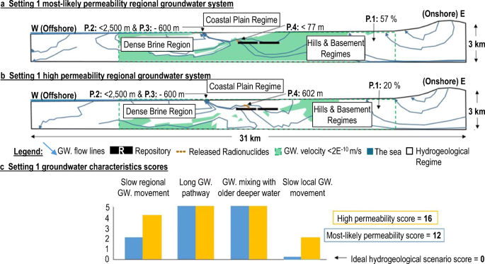
Regional groundwater system of setting 1 a when modelled with most-likely permeability values, and b when modelled with high permeability values. c Bar chart presenting beneficial groundwater characteristics scores for the most likely permeability (blue) and high permeability (yellow) modelled scenarios

Setting 2: key hydrogeological parameters score
-
P.1. 66% of the 20 × 2 km-far-field area exhibits very low rates of advective groundwater movement (see section ‘Methods’). This reduces to 39% when simulated with high permeability values.
-
P.2. Both high and most-likely permeability model simulations indicate long groundwater pathways of >13,700 m from repository to model boundary.
-
P.3. In both high and most-likely permeability models, pathways descend >1.6 km from the repository, and discharge to the onshore (northeast) boundary.
-
P.4. Both high and most-likely permeability model simulations indicate released radionuclides travel small distances over 10,000 years i.e. slow enough to be via diffusion (defaulted to <77 m, see section ‘Methods’). Released radionuclides would take at least 35,000 years to leave the host rock formation.
-
Overall score. Setting 2 accrues 3 and 4 out of 20 negative points for the most-likely and high permeability modelled scenarios respectively (Fig. 5c).
Fig. 5 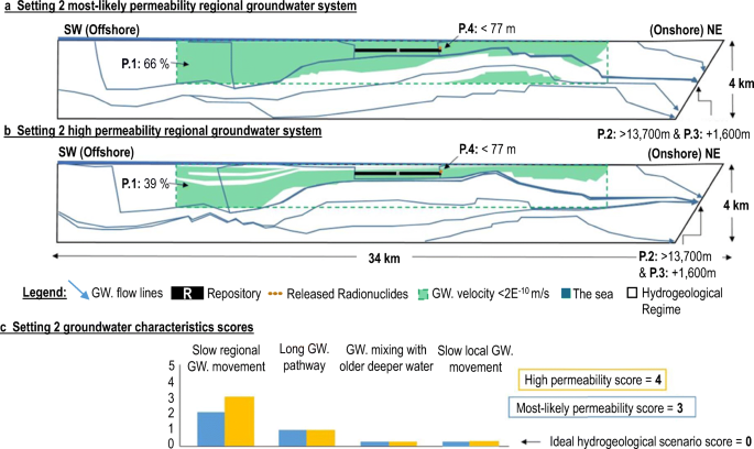
Regional groundwater system of setting 2 a when modelled with most-likely permeability values, and b when modelled with high permeability values. c Bar chart presenting beneficial groundwater characteristics scores for the most likely permeability (blue) and high permeability (yellow) modelled scenarios

Setting 3: key hydrogeological parameters score
-
P.1. 56% of the 20 × 2 km far-field area exhibits very low rates of advective groundwater movement (see section ‘Methods’). This reduces to 47% when simulated with high permeability values.
-
P.2. When modelled with most-likely permeabilities the setting shows long groundwater pathways (12,900 m). When modelled with high permeabilities, two pathways form. The first is similar to the most likely permeability model (13,000 m). The second however is shorter at 3100 m.
-
P.3. When modelled with most-likely permeabilities the groundwater pathway descends (150 m) from the repository and discharge to the west-northwest boundary (Fig. 6a). When modelled with high permeabilities, the first pathway is similar to the most likely permeability model descending (183 m) from the repository and discharge to the west-northwest boundary (Fig. 6b), however, the second ascends 630 m directly to the surface.
-
P.4. When modelled with most-likely permeabilities released radionuclides travel 375 m in 10,000 years i.e. remaining within the host rock (Fig. 6a). When modelled with high permeabilities, released radionuclides travel 5574 m (Fig. 6b) along the first pathway, remaining within the host rock formation, but 3100 m along the second pathway, discharging to the surface and exiting the model.
-
Overall score. Setting 3 accrues 7 and 16 out of 20 negative points for the most-likely and high permeability modelled scenarios respectively (Fig. 6c). The scoring for the high permeability scenario is based on the second ascending pathway as this is deemed of greatest risk from a safety perspective.
Fig. 6 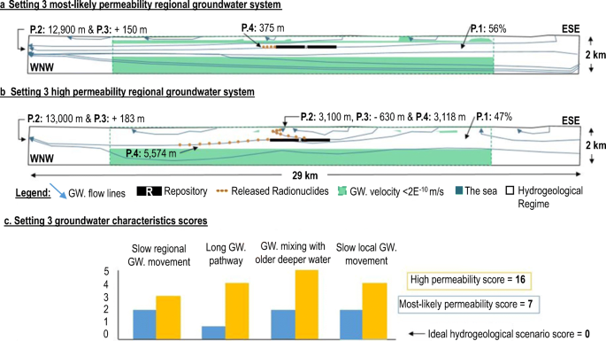
Regional groundwater system of setting 3 a when modelled with most-likely permeability values, and b when modelled with high permeability values. c Bar chart presenting beneficial groundwater characteristics scores for the most likely permeability (blue) and high permeability (yellow) modelled scenarios

Discussion
Setting 1: hydrogeological characteristics and performance potential
The regional groundwater flow pattern of setting 1 is controlled by enhanced topographic elevation (Lake District Fells) to the east, driving less dense rainfall derived groundwater westwards. The westward groundwater progression is blocked by the offshore dense ‘Irish Sea Brine’ regime, formed over millions of years from the dissolution of offshore salt rich layers (Bath et al. 1996; Black and Brightman 1996), which block and then forces groundwater up through the vicinity of the repository. This pattern of regional flow causes short and undesirable groundwater pathways (HC.2), which progress directly to the surface (HC.3).
The direct coupling between near-surface and deep groundwater (HC.6) is undesirable from a containment perspective and means that setting 1 cannot be considered analogous to the basement rock beneath sedimentary cover type HR (see Fig. 1). In addition, the direct coupling is likely to increase deep groundwater vulnerability to glacial flushing. This is supported by research from West Cumbria which attributes the high hydraulic heads presently observed in the Borrowdale Volcanic Group (basement rock) to be from the late Devensian glacial retreat (Black and Barker 2015), suggesting hydraulic coupling.
The host rock formation (lithological formation in which the engineered facility is constructed) is only likely to have wide spread diffusion-dominated (concentration driven, Domenico and Schwartz 1997) solute transport, which is desirable for radionuclide containment (Apted and Ahn 2017; Domenico and Schwartz 1997; Streffer et al. 2011), if field permeabilities are closest to the most-likely permeability range (HC.1 and HC.4). This indicates a lack of predictability (HC.5) in the potential performance of the setting (20% variation in overall score results), despite the extensive ground investigations previously undertaken for the RCF. Furthermore, the regional flow rates are fastest (~1.00E-07 to 1.00E-08 m s−1) within the overlying sedimentary sequence through which radionuclides will ultimately ascend, speeding up final discharge times (HC.1). Based on the overall score, setting 1 cannot be expected to exhibit broad ranging beneficial hydrogeological characteristics deemed advantageous for long term waste containment and isolation.
Setting 2: hydrogeological characteristics and performance potential
The regional groundwater flow pattern of setting 2 is primarily controlled by the groundwater density difference between the host rock formation and underlying units, and the constant pressure head from the sea, facilitating flow north-eastwards. These environmental conditions create long groundwater pathways from repository to model boundary (HC.2), which progress deeper into the earth rather than shallower (HC.3). These characteristics are advantageous from a performance perspective as they allow more time for radionuclide decay, and would also provide additional safety functions in the case of unknown geometric and lithological uncertainties, such as faults.
The high offshore chloride content (mass density) in setting 2 (Barnes et al. 2005; Bastin et al. 2003; Cowan and Boycott-Brown 2003; Yaliz and Chapman 2003; Yaliz and McKim 2003; Yaliz and Taylor 2003) is purportedly from dissolution of halite rich Mercia Mudstone Group layers (Barnes et al. 2005; Bath et al. 1996). Groundwater residence times have been reported as 2 million years for this Irish Sea Brine formation (Bath et al. 2006), which exceeds performance assessment timescales (1 million years; NDA 2014). Although dense brine formations can occur onshore (Bein and Arad 1992; Fritz and Frape 1982), the proximity from the coastline supports formation. This is because with distance from the coast, pressure (topographic) driven flow reduces, and very long duration geological processes, such as compaction, diagenesis, cementation, and mechanical stress, begin to dominate fluid flow (Bjørlykke 1993, 1994; Bjørlykke and Høeg 1997; Gluyas and Swarbrick 2003). Under these conditions, groundwater moves at velocity orders of magnitude slower than onshore (Bjørlykke 1993; Bjørlykke and Høeg 1997; Ge et al. 2003), with gases and waters diffusing extraordinarily slowly (Lu et al. 2009, 2011). Dense brines have also been found to reduce the upwards vertical velocity of groundwater under flushing conditions (Johns and Resele 1997; Park et al. 2009), providing hydrogeologically stable environments over inter-glacial timeframes (Park et al. 2009).
In support of this, modelling of setting 2 suggests that regardless of permeability uncertainty, the host rock formation is likely to transport solutes via diffusion (HC.4), whilst advection could only dominate solute transport in the underlying sedimentary sequence (Fig. 5a,b; HC.1). The overall scores (only 5% variation in results) shows a degree of predictability in the potential performance (HC.5), despite the setting having never been drilled to depth and thus shows promise.
It would however be beneficial for any future research to focus on the uncertain impact of glaciation on this groundwater system, especially as some degree of near-surface to deep groundwater coupling occurs in the model simulations (HC.6). Finally, simulation of setting 2 shows flow lines to descend through the low permeability sedimentary layers, and not along them. Setting 2 cannot therefore be considered directly analogous to the previously hypothesised ‘seaward dipping and offshore sediments’ HR (Fig. 1). However, based on the overall score, this location indicates broad ranging beneficial HCs for long-term waste containment and isolation, and thus warrants further investigation. Discussion of the wider implication of offshore deep geological disposal facility development is presented in section ‘Comparison of performance potential and wider implications and considerations’.
Setting 3: hydrogeological characteristics and performance potential
The regional groundwater flow pattern of setting 3 is sensitive to permeability uncertainty (45% variation in overall score results) (HC.5). In the most-likely permeability model, the overlying sedimentary layers behave as a low permeability seal preventing near-surface to deep groundwater coupling (HC.6). This creates a long horizontal groundwater pathway through the host rock (HC.2 and HC.3) and is thus desirable from a hydrogeological performance perspective. In the high permeability model however, the seal is ineffective and a direct coupling between near-surface and deeper groundwater occurs (HC.6), permitting radionuclide transport along a short ascending pathway to the surface (HC.2 and HC.3). This coupling is undesirable and again could create vulnerability to glacial flushing.
Regardless of permeability uncertainty, the models indicate released radionuclides to be transported via advection within the host rock (HC.4), and with diffusion-dominated transport only likely to become effective deeper within the host rock formation, or within the overlying sedimentary sequence (HC.1).
Because of the coupling, setting 3 can only be considered analogous to the basement rock beneath sedimentary cover HR (Fig. 1) if regional lithological permeabilities are closest to modelled most-likely values, but in comparison to setting 1, setting 3 does show a regional-scale resemblance to a basement rock beneath sedimentary cover regime.
The overall score reflects the uncertainty in site performance with setting 3 only exhibiting wide-ranging positive characteristics for radionuclide containment if the sedimentary sequence permeabilities are found to be closest to most-likely values. The permeability of the overlying sedimentary sequence should therefore be a key focus for any future investigation in this area.
Comparison of performance potential and wider implications and considerations
Modelling and assessment of the three exemplar groundwater settings shows the diverse quality of hydrogeological characteristics (i.e. groundwater speed and direction) available to be part of a comprehensive multi-barrier containment facility. For example, the overall scores indicate that setting 2 could exhibit hydrogeological characteristics (listed in section ‘The benchmark scenario’) that are 4 times more advantageous for long-term waste containment and isolation than setting 1 (see Fig. 7), i.e. when populated with most-likely permeabilities, setting 2 received an overall score of 3, which is four times more advantageous than that of setting 2 which received a score of 12. Similarly, when populated with high permeability values, setting 2 received a score of 4, which is four times better than the 16 received by setting 1.

Comparison of the far-field hydrogeological characteristics of the three selected sites using the newly proposed method of assessment. Setting 2 exhibits significantly more advantageous hydrogeological characteristics for the long-term containment and isolation of radionuclides than settings 1 or 3, despite uncertainties in permeability
The low score of setting 2 (close to the idealised scenario score of 0) is due to the settings’ long groundwater pathways, and slow local flow rates. These hydrogeological characteristics are due, in part, to its offshore location, the characteristics of which are discussed in section ‘Setting 2: hydrogeological characteristics and performance potential’. The apparent hydrogeological advantage of offshore settings for enhanced repository performance should be of interest to nation states with abundant offshore territory. Indeed, in 2016, RWM (the UK implementor) extended the search area for a GDF up to 20 km offshore the UK (RWM 2016b), which makes this research directly applicable.
Although the UK is the first country to publicly consider disposing of its high-level waste legacy offshore (both Sweden and Finland are constructing onshore GDFs (Posiva Oy 2012, 2017; SKB 2009)), the Swedish Final Repository (SFR) for short-lived intermediate and low-level waste was constructed under the Baltic Sea floor (SKB 2017, 2018). An extension of the SFR from 60 to 120 m below sea level is also planned (SKB 2018). The construction of the SFR, in addition to major international subseabed tunnels and mines sites including Boulby Potash Mine and the Channel Tunnel, indicate engineering feasibility. Offshore disposal could also speed up final disposal. This is because, in the UK, territorial waters are under the jurisdiction of the Crown Estate (Crown Estate 2017) who could become the sole party with whom approval for site investigations would be required. This could bypass the need for a volunteering host community which is stipulated by the NDA (2014). Technical challenges could however arise in designing appropriate ventilation systems (Parsons Brinckerhoff 2010), ensuring the retrievability of the waste if required, and public acceptability (Nirex 2005b).
Any site(s) identified for final disposal would be required to go through a rigorous safety assessment (IAEA 2009). This proposed assessment method is not intended as a safety assessment but is instead designed as a scoping tool for use at an early stage of site selection process to identify sites, with wide-ranging advantageous groundwater characteristics, determined by the proposed assessment method. By combining the scoping tool with pre-existing geological and hydrogeological data, the cost of site investigations can be minimised as settings with greatest performance potential (e.g. setting 2 which scored 3 and 4 respectively), and features within those settings most pertinent to safety (e.g. setting 3 cover rock permeability), can be focused upon.
It is understood that both technical and nontechnical factors will be involved in the site selection process; however, identification of advantageous natural settings should be at the forefront of the process because although the engineered barrier can be adapted for performance, the natural barrier cannot. Ultimately the natural barrier will be the main operational barrier preventing radionuclide return to the surface (RWM 2016a).
Timescales of natural barrier control have the potential to transcend interglacial timeframes (IAEA 2011b; greater than tens of thousands of years, Clark et al. 2012), which can exert significant forces on groundwater systems (Degnan et al. 2005; McEvoy et al. 2016; Tóth 1963; Tsang and Niemi 2013). Although this assessment method does not directly assess hydrogeological performance through glacial events, it does identify sites that at present show promise, and thus warrant further investigation for future features, events and process (McEvoy et al. 2016) resilience. However, even with advanced site investigations, significant aleatoric and epistemic uncertainty (see section ‘Method uncertainties’) remains. The magnitude of uncertainty is such that a ‘good enough’ site would be difficult to define. The best opportunity for performance success, despite these uncertainties, lies with selection of a high-quality natural barrier setting (comprising multiple advantageous characteristics) which operate in conjunction with a complimentary engineered barrier system. It is this concept that underpins the multi-barrier safety philosophy (IAEA 2009, 2011a), prevents overreliance on a single operational barrier function (IAEA 2011a), and ultimately drives this research.
This assessment method provides a high-level measure of the margin of hydrogeological advantage/disadvantage between settings. It is the belief of the authors that this type of quantitative measure would aid decision making by stakeholders and the public—with whom a final test of support is made (NDA 2014)—and reduce the risk of a ‘poor quality’, or ‘marginal’, site being selected.
Finally, the range of overall scores of the three exemplar settings are testament to the diversity of hydrogeological regimes present within the UK (Fig.7). This contrasts with Sweden and Finland which are both dominated by ‘low-lying fracture crystalline basement’ hydrogeological regimes (Posiva Oy 2012, 2017; SKB 2009) of the Baltic Shield. The diversity of UK natural barrier systems should be considered a resource and an opportunity for improved long-term repository performance, and should be explored as such.
Conclusion
A method is presented to assess and score the likely performance of any regional groundwater setting, which is required as part of a comprehensive multi-barrier deep geological disposal facility. This paper demonstrates how the assessment method, which is based on individual groundwater characteristics (such as speed and direction), can be used in conjunction with publicly available geological and hydrogeological data to score settings for prospectivity at an early stage of the site selection process. The method also enables identification of hydrogeological features, within assessed settings, that are most pertinent to performance. Using three UK settings as a case study, the approach indicates a significant difference (quantified as a fourfold variation) in the performance potential of difference regional groundwater settings to ensure long-term waste containment and isolation. Further research should focus on the settings identified here as showing the greatest prospective performance potential. Highlighted is the broad-ranging advantageous hydrogeological characteristics exhibited by the exemplar offshore setting.
References
Akhurst MC, Chadwick RA, Holliday DW, McCormac M, McMillian AA, Millward D, Young B, Ambrose K, Auton CA, Barclay WJ, Barnes RP, Beddoe-Stephens B, James JWC, Johnson H, Jones NS, Gover BW, Hawkins MP, Kimbell GS, MacPherson KAT, Milodowski AE, Riley NJ, Robins NS, Stone P, Wingfield RTR (1997) Geology of the West Cumbria District. Memoir of the British Geological Survey, sheets 28, 37 and 47 (England and Wales). British Geological Survey, Keyworth, UK
Andersson J, Staub I, Knight L (2005) Approaches to upscaling thermo-hydro-mechanical processes in fractures rock mass and its significance for large-scale repository performance assessment. Summary of findings in BMT2 and WP3 of DECOVALEX/BENCHPAR. Report, SKI report no. 2005-27, SKI, Stockholm, Sweden
Anderson MP, Woessner WW (1992) Applied groundwater modelling: simulation of flow and advective transport. Academic, San Diego, CA
ANDRA (2005) Dossier 2005 Argile: safety evaluation of a geological repository. Report series, ANDRA, Châtenay-Malabry, France
Apted MJ, Ahn J (2017) Geological repository systems for safe disposal of spent nuclear fuels and radioactive waste, 2nd edn. Woodhead, Duxford, UK
Atkins P (2001) The elements of physical chemistry: with applications in biology, 3rd edn., chap 16. Oxford University Press, Oxford, UK
Barnes RP, Chadwick RA, Darling WG, Gale IN, Kirby GA Kirk KL (2005) Contribution to Nirex review of a deep brine repository concept. BGS commissioned report, CR/05/230N, British Geological Survey, Keyworth, UK
Bastin JC, Boycott-Brown T, Sims A, Woodhouse R (2003) The South Morecambe Gas Field, blocks 110/2a, 110/3a, 110/7a and 110/8a, East Irish Sea. United Kingdom Oil and Gas Fields, Commemorative millennium volume, 20, Geological Society, London, pp 107–120
Bath AH, McCartney R, Richards H, Metcalfe R, Crawford MB (1996) Groundwater chemistry in the Sellafield area: a preliminary interpretation. Q J Eng Geol 29:30–57
Bath AH, Richards H, Metcalfe R, McCartney R, Degnan P, Littleboy A (2006) Geochemical indicators of deep groundwater movements at Sellafield, UK. J Geochem Explor 90:24–44
Bein A, Arad A (1992) Formation of saline groundwaters in the Baltic region through freezing of seawater during glacial periods. J Hydrol 40:75–87
Berry JA, Baker AJ, Bond KA, Cowper MM, Jefferies NL, Linklater CM (1999) The role of sorption onto rocks of the Borrowdale Volcanic Group in providing chemical containment for a potential repository at Sellafield. In: Metcalfe R Rochelle CA (eds) (1999) Chemical containment of waste in the geosphere. Geol Soc Lond Spec Publ 157:101–116
Bjørlykke K (1993) Fluid flow in sedimentary basins. Sediment Geol 86:137–158
Bjørlykke K (1994) Fluid-flow processes and diagenesis in sedimentary basins. In: Parnell J (ed) (1994) Geofluids: origin, migration and evolution of fluids in sedimentary basins. Geol Soc Lond Spec Publ 78:127–140
Bjørlykke K, Høeg K (1997) Effects of burial diagenesis on stresses, compaction and fluid flow in sedimentary basins. Mar Pet Geol 14(3):267–276
Black JH, Barker JA (2015) The puzzle of high heads beneath the West Cumbrian coast, UK: a possible solution. Hydrogeol J 24:439–457. https://doi.org/10.1007/s10040-015-1340-4
Black JH, Brightman MA (1996) Conceptual model of the hydrology of Sellafield. Q J Eng Geol 29:83–93
British Geological Survey (BGS) (1976) Hydrogeological map of North East Anglia: sheet 1 regional hydrological characteristics and explanatory notes. BGS, Keyworth, UK
British Geological Survey (BGS) (1997) Bootle, England and Wales sheet 47. Solid and drift geology, 1:50 000 series, BGS, Keyworth, UK
British Geological Survey (BGS) (1999a) Gosforth, England and Wales sheet 37. Solid Geology, 1:50 000 series, BGS, Keyworth, UK
British Geological Survey (BGS) (1999b) Swaffham, England and Wales sheet 160. Solid and drift geology, 1:50 000 series, BGS, Keyworth, UK
Chapman NA, McEwen TJ, Beale H (1986) Geological environments for deep disposal of intermediate level wastes in the United Kingdom. In: Siting, design and construction of underground repositories for radioactive wastes. Proceedings of a symposium, Hannover, Germany, 3–7 March 1986, International Atomic Energy Agency, Vienna, pp 311–328
Clark CD, Hughes ALC, Greenwood SL, Jordan C, Petter Sejrup H (2012) Pattern and timing of retreat of the last British-Irish ice sheet. Quat Sci Rev 44:112–146. https://doi.org/10.1016/j.quascirev.2010.07.019
Colley S, Thompson J (1991) Migration of uranium daughter radionuclides in natural sediments. Report no. 276, Institute of Oceanographic Sciences Deacon Laboratory, Wormley, UK
Corkhill CL, Cassingham NJ, Heath PG, Hyatt NC (2013) Dissolution of UK high-level waste glass under simulated hyperalkaline conditions of a colocated geological disposal facility. Int J Appl Glas Sci 4(4):341–356
Cowan G, Boycott-Brown T(2003) The North Morecambe field, block 110/2a, East Irish Sea. In: Gluyas JG, Hichens HM (eds) (2003) United Kingdom oil and gas fields commemorative millennium volume, 20. Geological Society, London, pp 97–105
Degnan P, Bath A, Cortés A, Delgado J, Haszeldine S, Milodowski A, Puigdomenech I, Recreo F, Šilar J, Torres T, Tullborg E-L (2005) PADAMOT: project overview report. PADAMOT Project technical report, United Kingdom NIREX, Chilton, UK, 105 pp
Department for Business, Energy and Industrial Strategy (BEIS) (2017) Digest of United Kingdom energy statistics 2017. National Statistics publication, July 2017, BEIS, London
Domenico PA, Schwartz FW (1997) Physical and chemical hydrogeology, 2nd edn. Wiley, Chichester, UK
Downing RA, Gray DA (1986) Geothermal resources of the United Kingdom. J Geol Soc London 143(3):499–507
Environment Agency (2009) Geological disposal facilities on land for solid radioactive wastes: guidance on requirements for authorisation February 2009’. Environment Agency, London
Environment Agency (2018) The Environment Agency’s approach to groundwater protection. February 2018 Version 1.2, Environment Agency, London
Falck WE, Hooker PJ (1990) Quantitative interpretation of Cl, Br and I porewater concentration profiles in lake sediments of Loch Lomond, Scotland. Commission of the European Communities; Nuclear Science and Technology. EC, Brussels
Fraser-Harris AP, McDermott CI, Kolditz O, Haszeldine RS (2015) Modelling groundwater flow changes due to thermal effects of radioactive waste disposal at a hypothetical repository site near Sellafield, UK. Environ Earth Sci 74(2):1589–1602
Fritz P, Frape SK (1982) Saline groundwaters in the Canadian Shield: a first overview. In: Geochemistry of radioactive waste disposal. Chem Geol 36(1–2):179–190
Ge S, Bekins B, Bredehoeft J, Brown K, Davis EE, Gorelick SM, Henry P, Kooi H, Moench AF, Rupel C, Sauter M, Screaton E, Swart PK, Tokunaga T, Voss CI, Whitaker F (2003) Fluid flow in sub-sea floor processes and future ocean drilling. EOS Trans Am Geophys Union 84(16):151–152
Geuzaine C, Remacle J-F (2009) Gmsh: a three-dimensional finite element mesh generator with built-in pre- and post-processing facilities. Int J Numer Methods Eng 79(11):1309–1331
Gin S (2014) Open scientific questions about nuclear glass corrosion. Procedia Materials Sci 7:163–171
Gluyas J, Swarbrick R (2003) Petroleum geoscience, 2nd edn. Blackwell, London
Grasshoff K, Kremling K, Ehrhardt M (1999) Methods of seawater analysis, 3rd edn. Wiley-VCH, Chichester, UK
Hipkins EV (2018) Comparing the hydrogeological prospectivity of three locations for deep radioactive waste disposal. https://www.era.lib.ed.ac.uk/handle/1842/33147. Accessed May 2020
Hudson JA, Stephansson O, Andersson J (2005) guidance on numerical modelling of thermo-hydro-mechanical coupled processes for performance assessment of radioactive waste repositories. Int J Rock Mech Min Sci 42(5–6):850–870
International Atomic Energy Agency (IAEA) (2009) Safety assessment for facilities and activities. IAEA safety standards, General safety requirements, part 4, IAEA, Vienna, Austria
International Atomic Energy Agency (IAEA) (2011a) Disposal of radioactive waste. IAEA safety standards, Specific safety requirements no. SSR-5, IAEA, Vienna, Austria
International Atomic Energy Agency (IAEA) (2011b) Geological disposal facilities for radioactive waste. IAEA safety standards, Specific safety guide no. SSG-14, IAEA, Vienna, Austria
Istok J (1989) Groundwater modelling by the finite element method, 1st edn. American Geophysical Union, Washington, DC
Jackson DI, Jackson AA, Evans D, Wingfield RTR, Barnes RP, Arthur MJ (1995) United Kingdom offshore regional report: the geology of the Irish Sea. British Geological Survey, London
Jackson DI, Johnson H, Smith JP (1997) Stratigraphical relationships and a revised lithostratigraphical nomenclature for the Carboniferous, Permian and Triassic rocks of the offshore East Irish Sea Basin. In: Meadows NS, Trueblood SP, Hardman M, Cowan G (eds) (1997) Petroleum geology of the Irish Sea and adjacent areas. Geol Soc Spec Publ 124:11–32
Jackson DI, Mulholland P, Jones S, Warrington G (1987) The geological framework of the East Irish Sea Basin. In: Brooks J, Glennie KW (1986) Petroleum geology of North West Europe. Proceedings of the 3rd Conference, London, 26–29 October 1986, pp 191–204
Joint Nature Conservation Committee (2003) Irish Sea Pilot: bottom temperature (Dec–Feb). Joint Nature Conservation Committee, Peterborough, UK
Johns RT, Resele G (1997) Solution and scaling of one-dimensional groundwater-solute flow with large density variations. Water Resour Res 33(6):1327–1334
King F, Sanderson D, Watson S (2016) Durability of high level waste and spent fuel disposal containers: an overview of the combined effect of chemical and mechanical degradation mechanisms. Technical report 17697-TR-03, Radioactive Waste Management. https://rwm.nda.gov.uk/publication/durability-of-high-level-waste-and-spent-fuel-disposal-containers/. Accessed May 2020
Kolditz O, Görke UJ, Shao H, Wang W (2012) Thermo-hydro-mechanical-chemical processes in porous media: benchmarks and examples. Lecture Notes in Computational Science and Engineering, vol 86., Springer, Heidelberg, Germany
Kolditz O, Bauer S, Bilke L, Böttcher N, Delfs JO, Fisher T, Görke UJ, Kalbacher T, Kosakowski G, McDermott CI, Park CH, Radu F, Rink K, Shao H, Shao HB, Sun F, Sun YY, Singh AK, Taron J, Walther M, Wang W, Watanabe N, Wu Y, Xie M, Xu W, Zehner B (2012) OpenGeoSys: an open-source initiative for numerical simulation of thermo-hydro-mechanical/chemical (THM/C) processes in porous media. Environ Earth Sci 67(2):589–599
Konikow LF, Bredehoeft JD (1992) Ground-water models cannot be validated. Adv Waste Resour 15(1):75–83
Lee K, Fetter CW (1994) Hydrogeology laboratory manual, 1st edn. Prentice Hall, Upper Saddle River, NJ
Lee JR, Woods MA, Morrlock BSP (eds) (2015) British regional geology: East Anglia, 5th edn. British Geological Survey, Keyworth, UK
Lide DR (ed) (2004) CRC handbook of chemistry and physics, 85th edn. CRC, Boca Raton, FL
Lu J, Wilkinson M, Haszeldine RS, Boyce AJ (2011) Carbonate cements in Miller field of the UK North Sea: a natural analog for mineral trapping in CO2 geological storage. Environ Earth Sci 62(3):507–517
Lu J, Wilkinson M, Haszeldine RS, Fallick AE (2009) Long-term performance of a mudrock seal in natural CO2 storage. Geology 37(1):35–38
McDermott CI, Randriamanjatosoa ARL, Tenzer H, Kolditz O (2006) Simulation of heat extraction from crystalline rocks: the influence of coupled processes on differential reservoir cooling. Geothermics 35(3):321–344
McEvoy FM, Schofield DI, Shaw RP, Norris S (2016) Tectonic and climatic considerations for deep geological disposal of radioactive waste: a UK perspective. Sci Total Environ 571:507–521
McKeown C, Haszeldine RS, Couples GD (1999) Mathematical modelling of groundwater flow at Sellafield, UK. Eng Geol 52(3–4):231–250
Metcalfe R, Crawford MB, Bath AD, Littleboy AK, Degnan PJ, Richards HG (2007) Characteristics of deep groundwater flow in a basin marginal setting at Sellafield, Northwest England: 36Cl and halide evidence. Appl Geochem 22(1):128–151
Metcalfe R, Watson SP, Rees JH, Humphreys P, King F (2008) Gas generation and migration from a deep geological repository for radioactive waste: a review of Nirex/NDA’s work. Technical report no. NWAT/NDA/RWMD/2008/002, Environment Agency, London
Michie U (1996) The geological framework of the Sellafield area and its relationship to hydrogeology. Q J Eng Geol Hydrogeol 29:S13–S27
Miller W, Alexander R, Chapman N, McKinley I, Smellie J (1994) Natural analogues studies in the geological disposal of radioactive waste. Technical Report 93–03, National Cooperative for the Disposal of Radioactive Waste, Wettingen, Switzerland
Nagra (2002) Opalinus Clay Project: demonstration of feasibility of disposal for spent fuel, vitrified high-level waste and long-lived intermediate-level waste. Summary overview document, National Cooperative for the Disposal of Radioactive Waste, Wettingen, Switzerland
Niemi A, Yang Z, Carrera J, Power H, McDermott CI Rebscher D, Wolf JL, May F, Figueiredo B, Vilarrasa V (2017) Mathematical modelling: approaches for model simulation’. In: Niemi A, Bear J, Bensabat J (eds) (2017) Geological storage of CO2 in deep saline aquifers. Springer, Heidelberg, Germany, pp 144–150
Nirex (1997a) An assessment of the post-closure performance of a deep waste repository at Sellafield, vol 1: hydrogeological model development—conceptual basis and data. Report no. S/97/012, United Kingdom Nirex, Harwell, UK
Nirex (1997b) An assessment of the post-closure performance of a deep waste repository at Sellafield, vol 2: hydrogeological model development: effective parameters and calibration. Report no. S/97/012, United Kingdom Nirex, Harwell, UK
Nirex (1997c) An assessment of the post-closure performance of a deep waste repository at Sellafield, vol 3: the groundwater pathway. Report no. S/97/012, United Kingdom Nirex, Harwell, UK
Nirex (1997d) An assessment of the post-closure performance of a deep waste repository at Sellafield, vol 4: the gas pathway. Report no. S/97/012, United Kingdom Nirex, Harwell, UK
Nirex (2002) Options for radioactive waste management that have been considered by Nirex. Report no. N/049, United Kingdom Nirex, Harwell, UK
Nirex (2005a) Review of 1987–1991 site selection for an ILW/LLW repository. Report no. 477002, United Kingdom Nirex, Harwell, UK
Nirex (2005b) Review of CoRWM document no. 625: sub seabed disposal. Report no. 471699, United Kingdom Nirex, Harwell, UK
Nuclear Decommissioning Authority (NDA) (2010a) Geological disposal: generic environmental safety case main report. NDA report no. NDA/RWMD/021, Nuclear Decommissioning Authority, Moor Row, UK
Nuclear Decommissioning Authority (NDA) (2010b) Geological disposal: radionuclide behaviour status report. NDA report no. NDA/RWMD/034, Nuclear Decommissioning Authority, Moor Row, UK
Nuclear Decommissioning Authority (NDA) (2010c) Geological disposal: an overview of the generic disposal system safety case. NDA report no. NDA/RWMD/010, Nuclear Decommissioning Authority, Moor Row, UK
Nuclear Decommissioning Authority (NDA) (2013) Geological disposal: Overview of international siting processes. September 2013, Nuclear Decommissioning Authority, Moor Row, UK
Nuclear Decommissioning Authority (NDA) (2014) Implementing geological disposal: a framework for the long-term management of higher activity radioactive waste. URN 14D/235, Department of Energy and Climate Change, London
Nuclear Decommissioning Authority (NDA) (2017) Radioactive wastes in the UK: UK radioactive waste inventory report. Department for Business, Energy & Industrial Strategy, London
OpenGeoSys (2017) OpenGeoSys: open-source multi-physics webpage. www.opengeosys.org/. Accessed December 2017
Park YJ, Sudicky EA, Sykes JF (2009) Effects of shield brine on the safe disposal of waste in deep geologic environments. Adv Water Resour 32(8):1352–1358
Parsons Brinckerhoff (2010) Geological disposal facility ventilation study. Radioactive Waste Management Directorate, Radioactive Waste Management, London
Posiva Oy (2012) Safety case for the disposal of spent nuclear fuel at Olkiluoto: synthesis 2012. Report no. POSIVA 2012–12, Possiva Oy, Eurajoki, Finland
Posiva Oy (2017) Final disposal webpage. www.posiva.fi/en/final_disposal#.WtBz02eWzoo. Accessed December 2017
Radioactive Waste Management (RWM) (2016a) Geological disposal: engineered barrier system status report. Report no. DSSC/452/01, Nuclear Decommissioning Authority, Moor Row, UK
Radioactive Waste Management (RWM) (2016b) Implementing geological disposal: providing information on geology, national geological screening guidance. Nuclear Decommissioning Authority, Moor Row, UK
Schlumberger (2016) Common data access: UKOilandGasData website. Accessed 2016 and 2017 via the University of Edinburgh, Edinburgh, Scotland
Sharland SM, Agg PJ, Naish CC, Wikramaratna RS (2008) Gas generation by metal corrosion and the implications for near-field containment in radioactive waste repositories. AEA Technology Group report, AEA, Oxfordshire, UK
SKB (2009) Final repository for spent fuel in Forsmark: basis for decision and reasons for site selection. SKBdoc 1221293 (English Translation of SKBdoc 1207622), Svensk Kärnbränslehantering, Stockholm
SKB (2017) The final repository SFR webpage. www.skb.com/our-operations/sfr/. Accessed December 2017
SKB (2018) Extending the SFR webpage. www.skb.se/upload/publications/pdf/Fact-sheet_Extending_the_SFR.pdf. Accessed December 2018
SOEST (2015) University of Hawaii at Manoa webpage. School of Ocean Earth Science and Technology. www.soest.hawaii.edu/oceanography/courses/OCN623/Spring2015/Salinity2015web.pdf. Accessed December 2018
Streffer C, Gethmann CF, Kamp G, Kröger W, Rehbinder E, Renn O (2011) Radioactive waste: technical and normative aspects of its disposal. Springer, Heidelberg, Germany
Tecplot (2018) Tecplot: home webpage. www.tecplot.com/. Accessed December 2018
The Crown Estate (2017) Energy, minerals and infrastructure: cables and pipelines. webpage (page removed 2018). http://www.thecrownestate.co.uk/en-gb/what-we-do/on-the-seabed/cables-and-pipelines/. Accessed December 2017
Tóth J (1963) A theoretical analysis of groundwater flow in small drainage basins. J Geophys Res 68(16):4795–4812
Tsang C-F, Niemi A (2013) Deep hydrogeology: a discussion of issues and research needs. Hydrogeol J 21(8):1687–1690
UK Parliament (1997) Town and Country Planning Act 1990: appeal by United Kingdom Nirex Limited proposed rock characterisation facility on land at and adjoining Longlands Farm, Gosforth, Cumbria (Local Authority Application Number 4/94/9011). Letter dated 17th March 1997, UK Parliament, London
University of Edinburgh (2018) High performance computing webpage. www.ed.ac.uk/information-services/research-support/research-computing/ecdf/high-performance-computing. Accessed December 2018
Watanabe N, Wang W, McDermott CI, Taniguchi T, Kolditz O (2010) Uncertainty analysis of thermo-hydro-mechanical coupled processes in heterogeneous porous media. Comput Mech 45(4):263–280
Wollenberg HA, Flexser S (1984) Contact zones and hydrothermal systems as analogues to repository conditions. In: Smellie J (ed) Natural analogues to the conditions around a final repository for high level radioactive waste. SKB technical report TR 84–18, SKB, Stockholm
Yaliz A, Chapman TJ (2003) The Lennox oil and gas field, block 110/15, East Irish Sea. In: Gluyas JG, Hichens HM (eds) (2003) United Kingdom oil and gas fields. Commemorative millennium volume, Memoir, vol 20, Geological Society, London, pp 87–96
Yaliz A, McKim N (2003) The Douglas oil field, block 110/13b, East Irish Sea. In: Gluyas JG, Hichens HM (eds) (2003) United Kingdom oil and gas fields. Commemorative millennium volume, Memoir, vol 20, Geological Society, London, pp 63–75
Yaliz A, Taylor P (2003) The Hamilton and Hamilton north gas fields, block 110/13a, East Irish Sea. In: Gluyas JG, Hichens HM (eds) (2003) United Kingdom oil and gas fields. Commemorative millennium volume, Memoir, vol 20, Geological Society, London, pp 77–86
Funding
This research was funded through the Natural Environment Research Council’s (NERC) E3 Doctoral Training Programme.
Author information
Authors and Affiliations
Corresponding author
Ethics declarations
Disclaimer
The settings assessed within this research were selected as a theoretical exercise due to their perceived hydrogeological differences and were constructed using publicly available geological data. The settings selected here are not, to the knowledge of the authors, under official investigation by the UK implementer.
The setting 1 model was developed from a model originally constructed by Fraser-Harris et al. 2015. Further information on this research, and the research undertaken by Fraser-Harris et al. 2015, can be found in Hipkins 2018.
Electronic supplementary material
ESM 1
(PDF 2126 kb)
Rights and permissions
Open Access This article is licensed under a Creative Commons Attribution 4.0 International License, which permits use, sharing, adaptation, distribution and reproduction in any medium or format, as long as you give appropriate credit to the original author(s) and the source, provide a link to the Creative Commons licence, and indicate if changes were made. The images or other third party material in this article are included in the article's Creative Commons licence, unless indicated otherwise in a credit line to the material. If material is not included in the article's Creative Commons licence and your intended use is not permitted by statutory regulation or exceeds the permitted use, you will need to obtain permission directly from the copyright holder. To view a copy of this licence, visit http://creativecommons.org/licenses/by/4.0/.
About this article

Cite this article
Hipkins, E.V., Haszeldine, R.S. & McDermott, C.I. Comparing the prospectivity of hydrogeological settings for deep radioactive waste disposal. Hydrogeol J 28, 2241–2257 (2020). https://doi.org/10.1007/s10040-020-02182-2
Received:
Accepted:
Published:
Issue Date:
DOI: https://doi.org/10.1007/s10040-020-02182-2