Parameterized verification of systems with component identities, using view abstraction

Abstract

The parameterized verification problem seeks to verify all members of some collection of systems. We consider the parameterized verification problem applied to systems that are composed of an arbitrary number of component processes, together with some fixed processes. The components are taken from one or more families, each family representing one role in the system; all components within a family are symmetric to one another. Processes communicate via synchronous message passing. In particular, each component process has an identity, which may be included in messages, and passed to third parties. We extend Abdulla et al.’s technique of view abstraction, together with techniques based on symmetry reduction, to this setting. We give an algorithm and implementation that allows such systems to be verified for an arbitrary number of components: we do this for both safety and deadlock-freedom properties. We apply the techniques to a number of examples. We can model both active components, such as threads, and passive components, such as nodes in a linked list: thus our approach allows the verification of unbounded concurrent datatypes operated on by an unbounded number of threads. We show how to combine view abstraction with additional techniques in order to deal with other potentially infinite aspects of the analysis: for example, we deal with potentially infinite specifications, such as a datatype being a queue; and we deal with unbounded types of data stored in a datatype.

1 Introduction

The parameterized verification problem considers a collection of systems P(x) where the parameter x ranges over a potentially infinite set, and asks whether such systems are correct for all values of x. In this paper we consider the following instance of the parameterized verification problem. Each system is built from some number of component processes, together with some fixed processes. The components may be taken from one or more families; for instance, we will consider examples representing a concurrent datatype based on a linked list: one family of components will represent threads operating on the datatype and another family will represent nodes in the linked list. All components from a particular family will be symmetric to one another. Thus these systems are parameterized by the number of components from each family. The fixed processes are independent of the number of components; we use them to model shared resources such as shared variables or locks; we also normally include a watchdog as a fixed process, which monitors the execution and signals an error if the desired specification is not met.

The components and fixed processes communicate via (CSP-style) synchronous message passing; we call each message an event. In particular, each component has an identity, drawn from some potentially infinite set. These identities can be included in events; thus a process can obtain the identity of a component process and possibly pass it on to a third process. This means that each process has a potentially infinite state space (a finite control state combined with identities from a potentially infinite set). We describe the setting for our work more formally in the next section. The problem (of showing that a system with n components is correct, for all n) is undecidable in general [9, 44]; however, verification techniques prove effective on a number of specific instances.

We adapt the technique of view abstraction of Abdulla et al. [4] to this setting. The idea of view abstraction is that we abstract each system state by its views, where each view records the states of the fixed processes, but just some subset of the components. For each analysis, we fix a set of views of interest; for example, we might consider all views containing precisely two component states (plus the fixed processes). We then calculate an upper bound on the set of such views of all reachable states of all systems of arbitrary size. By reasoning about this set of views, we can show that all such systems are correct.

The calculation proceeds as follows. Given a set S of views, we can (in principle) calculate the set of concrete states consistent with those views, i.e. those states st such that every view of st is in S; we call these concretizations. Informally (using the terminology of [6]), we “piece together” the views in S to create concretizations. We then calculate concrete transitions from those concretizations, and form the views of the resulting states. We repeat this process until we reach a fixed point: this fixed point provides the required upper bound described in the previous paragraph.

In fact, rather than considering all concretizations consistent with the set of views, it is enough to consider only concretizations that contain two components more than the views (so if all views are of size k, then the concretizations are of size $k+2$). We can improve the efficiency of the approach in the case that there are no three-way synchronizations between two components and a fixed process: it is enough to calculate concretizations that have a single component more than the views (so if all views are of size k, then the concretizations are of size $k+1$).

In [4] and our earlier work [40], the abstraction recorded all views of some size k, i.e. recording the states of k components in all possible ways. This approach works fine in principle, but on some examples suffers from a state space explosion: the number of views becomes prohibitive. In this paper, we generalise the approach to consider all views of certain profiles; for example, we might consider all views that record the states of two threads and one node, or one node and two threads. We present our use of view abstraction in Sects. 3 and 4.

Our setting is made more complicated by the use of component identities. These mean that the set of views (for some fixed collection of profiles) is potentially infinite. However, in Sect. 5 we use techniques from symmetry reduction [15, 17, 18, 24, 29, 37, 53] to reduce the views that need to be considered to a finite set. The idea is that if two views are equivalent modulo a uniform renaming of component identities, then the algorithm needs to consider only one of them.

We present the main algorithm for verifying safety properties in Sect. 6, and prove its correctness.

In Sect. 7, we extend our techniques to verify deadlock-freedom properties, i.e. that in every reachable state, at least one process is able to perform an action. Verifying such properties within view abstraction is not straightforward, since each concretization records only part of the global state: it might be that no component in the concretization can perform an action, but components outside the concretization can. We show that it is enough to consider only certain concretizations, which we term significant: if an action is possible in every significant concretization, then the same is true of every global state.

We present our implementation in Sect. 8: this is based upon the process algebra Communicating Sequential Processes (CSP) [50]. We use the model checker Failures Divergences Refinement (FDR) [28] as a back-end, to produce state machines for the components and fixed processes; this allows us to support all of machine-readable CSP@. We stress, though, that the main ideas of this paper are not CSP-specific: they apply to any formalism with a similar computational model, and, we believe, could be adapted to other computational models.

In Sect. 9, we present a range of examples, and experimental results. Being able to model process identities (or something equivalent) is necessary for all but one of the examples. Many examples present challenges beyond those of the unbounded number of processes. For instance, many examples operate on an unbounded domain of data values. For others, the requirements, such as being a queue, are naturally captured by an infinite-state specification. And in some cases, individual components may be infinite state and need to be abstracted. A number of techniques exist for tackling these challenges. We adapt and extend these techniques, using them in the models that we analyse with our tool.

A typical analysis combines abstractions in the model with the abstraction provided by the tool. Different examples require different abstraction techniques: we leave it up to the analyst to select the appropriate techniques in each case (but we hope our examples will provide guidance). It is our thesis that having the tool concentrate on just view abstraction makes that analysis more efficient, while the analyst can craft the model, tailoring it to the details of the example. (Of course, one could imagine another tool that helps the analyst craft the model, as part of a tool chain.)

In some examples, we use techniques from data independence, to capture the specification of the datatypes in a finite-state way. In particularly, we adapt Wolper’s specification technique for queues [60] and use a similar technique for stacks. We give techniques that can deal with non-fixed linearization points. In other examples, we adapt techniques of Henzinger et al. [16, 33].

Our examples include reference-linked data structures, such as linked lists. Each node in the data structure is modelled by a component process; such a process can hold the identity of another such process, modelling a reference to that node. Our examples include concurrent queues, stacks and sets, each based on a linked list (both lock-based and lock-free).

Other examples include a synchronous channel [41, 54], a multiplexed buffer, an elimination stack [32], a termination protocol for a ring, and a timestamp-based queue (inspired by [22]), that uses a number of subqueues internally (modelled as a family of components). The final example, in particular, requires the abstraction of the domain of timestamps, the abstraction of the subqueues, and a way for a thread to iterate over the subqueues.

By including views of a particular size k, our approach automatically captures invariants that concern the relationship between the states of (at most) k components and the fixed processes. For example, taking $k=2$ in an example using linked lists, we can capture the relationship between the states of any pair of nodes, including between any pair of adjacent nodes. This allows us to capture various invariants concerning the “shape” of the list; for example it can capture the invariant that the list holds a sequence of data from the language $A^*B^*$ (every pair of adjacent nodes hold data values (A, A), (A, B) or (B, B)).

In our examples based on linked lists, we will ensure that the sequence of data values held in the list comes from a language that: (1) can be captured using the type of invariant described in the previous paragraph, i.e. relating the values in successive nodes; and (2) allows us to prove that the relevant specification is met, using the data-independence techniques mentioned earlier. The approach does not automatically capture all properties, particularly transitivity properties such as that one node is reachable from another; however, we have developed modelling techniques that can often work around this.

Our approach is rather general and supports the analysis of a wide range of examples beyond those based on linked lists. The generality has a down-side though: the approach is not as fast as special-purpose techniques that are optimized for particular classes of problems, such as techniques targeted towards linked lists. Nevertheless, our approach gives acceptable performance.

We see our main contributions as follows.

• An adaptation of view abstraction to synchronous message passing (this is mostly a straightforward adaptation of the techniques of [4]);

• An extension of view abstraction to include systems where components have identities, and these identities can be passed around, using techniques based on symmetry reduction to produce a finite-state abstraction;

• The extension of view abstraction to consider just specific profiles of views;

• The extension of view abstraction in order to analyse for deadlock freedom;

• The implementation of these techniques in a powerful tool, using FDR so as to support all of machine-readable CSP;

• The application to a wide range of examples. These examples illustrate: (1) the adaptation and extension of techniques, using data independence, for specifying several datatypes; (2) the adaptation and extension of other abstraction techniques, to deal with other aspects of the models that would otherwise be infinite; (3) techniques for ensuring that the abstractions capture sufficiently strong invariants to prove correctness.

Compared to our earlier work [40], the main advances are: the extension to deal with deadlock freedom; a greatly improved implementation (reducing checking times by a factor of several hundred, and increasing the size of models checkable by a factor of several tens of thousands); extensions to allow multiple families of components, to consider just specific profiles, and to support three-way synchronizations between two components and a fixed process; and the application to a wider range of examples, together with the development of suitable specification and abstraction techniques.

1.1 Related work

There have been many approaches to the parameterized model checking problem.

Much recent work has been based on regular model checking, e.g. [14, 20, 39, 58]. Here, the state of each individual process is from some finite set, and each system state is considered as a word over this finite set; the set of initial states is a regular set; and the transition relation is a regular relation, normally defined by a transducer. An excellent survey is in [2]. Techniques include widening [55], acceleration [1] and abstraction [13].

The work [4] that the current paper builds on falls within this class. However, our setting is outside this class: the presence of component identities means that each individual process has a potentially infinite state space.

German and Sistla [27] consider a similar setting to us. They capture the correctness property via an LTL formula that considers the execution of the fixed processes and at most one component. They model a system using a vector addition system with states (VASS), which models explicitly the state of the fixed processes and of the specification automaton, and counts the number of components in each state. Again this is possible because each component is finite-state, unlike in our case. Existing algorithms can be used to decide relevant properties of a VASS, albeit in double-exponential time. They show that in the case of there being no controller, and for a specification automaton that monitors a single component, the problem is decidable in polynomial time. Despite the poor complexity result for the general case, subsequent works have produced tools that can cope with a number of examples, e.g. [3, 11, 21, 25, 38].

Other approaches include induction [23, 51], network invariants [59], and counter abstraction [19, 42, 44, 49]. In particular, [44] applied counter abstraction to systems, like in the current paper, where components had identities which could be passed from one process to another: some number B of the identities were treated faithfully, and the remainder were abstracted; the approach of the current paper seems better able to capture relationships between components, as required for the analysis of many examples.

Most approaches to symmetry reduction in model checking [15, 18, 24, 29, 37] work by identifying symmetric states, and, during exploration, replace each state encountered with a representative member of its symmetry-equivalence class: if several states map to the same representative, this reduces the work to be done. This representative might not be unique, since finding unique representatives is hard, in general; however, such approaches work well in most cases. Our approach follows this style, using unique representatives.

We discuss other techniques for specifying linearizability of various datatypes, different abstraction techniques, and other techniques for analysing datatypes based on a linked list in Sects. 9.14 and 9.15, where we are better able to compare with our own techniques.

2 The framework

In this section, we introduce more formally the class of systems that we consider, and our framework. Recall that we are interested in systems with an unbounded number of component processes, perhaps from different families, and some fixed processes.

We introduce two examples to illustrate the ideas. In our first, toy, example, the components run a simple token-based mutual exclusion protocol. Component j can receive the token from component i via a transition with event pass.i.j; it can then enter and leave the critical section, before passing the token to another component. In the initial state, a single component holds the token.

A watchdog (fixed) process observes components entering and leaving the critical section, and signals with event error if mutual exclusion is violated. Our correctness conditions will be that the event error does not occur and that the system does not deadlock. (The idea of using a watchdog is essentially the same as the automata-theoretic approach to model checking [57], where an automaton defines the allowable executions.)

Figure 1 illustrates state machines for these processes.

Fig. 1

Illustration of the state machines for the toy example: a component (above) and the watchdog (below). The diagrams are symbolic, and parameterized by the set of component identities. For example, the latter state diagram has a state $wd_1(id)$ for each identity id; there is a transition labelled enter.id from $wd_0$ to $wd_1(id)$ for each identity id. In the events labelling transitions, “?” indicates that the following field can take an arbitrary value; a parameter in the subsequent state may be bound to this value

Each process’s state is the combination of a control state and a vector of zero or more parameters, each of which is a component identity, either its own identity or that of another component. In particular, each component process stores its own identity as its first parameter. Likewise, each event is the combination of a channel name and zero or more component identities. Processes synchronise on common events; for example, components id and $id'$ synchronise on the event $pass.id.id'$. We make the restriction that at most two components and maybe some fixed processes synchronise on each event. We want to verify such systems for an arbitrary number of components.

Fig. 2

Pseudo-code for the lock-based stack example

Fig. 3

State machines for the lock-based stack example

Figure 3 gives a more interesting example, representing a lock-based stack that uses a linked list internally; pseudo-code is in Fig. 2. Here the components come from two families: nodes that make up the linked list; and threads that operate on the stack.

Each node hold a piece of data x, of some type D, and a reference next to the next node in the linked list, which might be a special value null. In the state machine, each node has an identity me from the type of node identities; x is treated as part of the control state and of the initializing channel, since it does not correspond to the identity of a component. We assume that the type D of data is finite (in Sect. 9 we use techniques from data independence to justify the use of finite types of data within our models).

The node can be initialized by a thread. Subsequently, a thread can get the value of next or x. In other similar examples, there might be additional transitions corresponding to a thread updating the next reference.

The datatype uses a lock, and a variable Top that points to the top node on the stack. Each thread performs push and pop operations upon the stack: the exact details aren’t important here. In the state machine, each thread component has an identity me from a type of thread identities. It synchronises with node components to initialise them, or to get their next or x fields. It synchronises with the lock to lock and unlock the datatype, and with Top to get or set a reference to the current top node in the stack. It performs additional signal events, $push_x.me$, $pop_x.me$ and popEmpty.me to indicate the operation it is performing and the result; we later use these to capture the property that the system implements a stack. In each state, each thread holds its own identity; in some states, it also holds a reference to a node.

The fixed processes are the lock and Top. For the purposes of the formal development, it is simplest to assume a single fixed process, which we can take as the product of the two parts. The state machine for the lock allows the datatype to be locked and unlocked. The state machine for Top stores a reference to the current top node, which threads may get or set. In Sect. 9, we describe how to extend the fixed processes to include a watchdog part that checks that the system does indeed implement a stack.

2.1 Processes

Formally, each process (a component or a fixed process) is represented by a parameterized state machine.

Definition 1

A state machine is a tuple $(Q, \Sigma , \delta )$, where: Q is a set of states; $\Sigma$ is a set of visible events with ($\tau$ represents an internal event); and is a transition relation.

Let T be some potentially infinite set T of component identities. A parameterized state machine over T is a state machine where:

• the states Q are a subset of , for some finite set S of control states;

• the events $\Sigma$ are a subset of , for some finite set Chan of channels.

We sometimes write a state $(s, \mathbf{x} )$ as $s(\mathbf{x} )$: s is a control state, and $\mathbf{x}$ records the values of its parameters (cf. Figs. 1 and 3). Similarly, we write an event as $c.\mathbf{y}$, and write to denote $((s, \mathbf{x} ), (c, \mathbf{y} ), (s', \mathbf{z} )) \in \delta$.

The type T of identities may be partitioned into one or more subtypes: in the linked-list-based stack example, T is partitioned into the subtypes of node identities and thread identities. Further, certain values may be distinguished, such as the value null representing the null node reference.

We assume that the states of a state machine are well typed in the sense that two states with the same control state have the same number and types of parameters: if $cs(x_1,\ldots ,x_n), cs(x_1',\ldots ,x_{n'}') \in Q$, then $n = n'$, and $x_i$ and $x_i'$ are from the same subtype, for each i. Likewise, we assume that the set of visible events is well typed.

We assume that the component identities are treated data independently: they can be received, stored, sent, and tested for equality; but no other operations, such as arithmetic operations, can be performed on them. Processes defined in this way are naturally symmetric, in a way that we now make clear.

Let $\pi$ be a permutation on T that maps each value to a value of the same subtype, and maps each distinguished value to itself; we write Sym(T) for the set of all such permutations. We lift $\pi$ to vectors from $T^*$ by point-wise application; we then lift it to states and events by $\pi (s(\mathbf{x} )) = s(\pi (\mathbf{x} ))$ and $\pi (c.\mathbf{x} ) = c.\pi (\mathbf{x} )$; we lift it to sets, etc., by point-wise application. We require each state $s(\pi (\mathbf{x} ))$ to be equivalent to $s(\mathbf{x} )$ but with all events renamed by $\pi$: formally the states are $\pi$-bisimilar [47].

Definition 2

Let $M = (Q, \Sigma , \delta )$ be a state machine, and let $\pi \in Sym(T)$. We say that $\mathord {\sim } \subseteq Q \times Q$ is a $\pi$-bisimulation iff $\pi (\Sigma ) = \Sigma$, and whenever $(q_1, q_2) \in \mathord {\sim }$ and :

• If then ;

• If then .

Definition 3

A parameterized state machine $(Q, \Sigma , \delta )$ is symmetric if for every ,  is a $\pi$-bisimulation.

The node and thread state machines in Fig. 3 are symmetric. For example, the states $Node_A(N_0, N_1)$ and $Node_A(N_1,N_4)$ are $\pi$-bisimilar for each $\pi \in Sym(T)$ with $\pi (N_0) = N_1$ and $\pi (N_1) = N_4$.

This notion of symmetry is a natural condition. In [29], we proved that an arbitrary process defined using machine-readable CSP will be symmetric in this sense under rather mild syntactic conditions, principally that the definition of the process contains no non-distinguished constant from the type T.

2.2 Systems

Each system will contain a fixed process and some number of components. We assume a single fixed process here, for simplicity: a system with multiple fixed processes can be modelled by considering the parallel composition of those processes as a single process.

Each system state contains a state for the fixed process, and a finite set containing the state for each component. For example, one state of the toy mutual-exclusion example is where . We start by defining the semantics of the components.

Definition 4

A component definition is a pair (Cpt, Sync) where

• 1. $Cpt = (Q_c, \Sigma _c, \delta _c)$ is a symmetric parameterized state machine over T, representing each component. Each component has an identity, represented by its first parameter; we define¹$\mathop {\mathsf {id}}(cs, p.ps) = p$. We require that the identity is a non-distinguished value, and that the identity does not change: if in $\delta _c$ then $\mathop {\mathsf {id}}(q) = \mathop {\mathsf {id}}(q')$.

• 2. $Sync \subseteq \Sigma _c$ is a set of events that require the synchronization of two components; we require $\pi (Sync) = Sync$ for each $\pi \in Sym(T)$, and .

A component definition defines a state machine²$(\mathbb {P}(Q_c), \Sigma _c, \delta )$ that represents all the components. The transition relation $\delta$ is defined by the following two rules, where corresponds to $\delta _c$; the rules represent, respectively, an event of just one component, and a synchronization between two components.

Note that the components may be of different families (such as threads and nodes): the different families correspond to different sets of states within $Q_c$. We assume that all components of the same family will have the same type for their identities (such as thread identities and node identities). However, in some examples it is necessary to have two families that use the same type for their identities; for example, in Sect. 9.3 we use two families, Thread and LockSupport, that use the same type ThreadID for their identities. The following definition captures the idea of families.

Definition 5

A family function is a function , where F is a finite set, and:

• The family of a component is preserved by transitions:

  

• For each family f, the identities of states of family q all have the same type; we denote this type (a sub-type of T):

  

Each component can be identified by the combination of its family and identity, which we term a process identity, of type . The function returns the process identity of a component:

(Including the family is necessary in the case that two families use the same types for their identities.)

Definition 6

A system definition is a tuple , where

• 1. T is a type, partitioned into subtypes $T_1,\ldots , T_n$;

• 2. $Fixed = (Q_F, \Sigma _F, \delta _F)$ is a symmetric parameterized state machine over T representing the fixed process;

• 3. $Cpts = ((Q_c, \Sigma _c, \delta _c), Sync)$ is a component definition over T;

• 4. is a family function over $Q_c$;

• 5. $Init \subseteq \mathcal {SS}$ is a set of initial states, where denotes all possible system states.

Given such a system, a system state is a pair $(q_F, m) \in \mathcal {SS}$, where ${q_F \in Q_F}$ gives the state of the fixed process, and $m \in \mathbb {P}(Q_c)$ gives the states of the components, where different components in m have distinct process identities.

A system definition defines a state machine , where $\delta$ is defined by the following three rules (where and correspond to $\delta _F$ and the transition relation of Cpts, respectively). The rules represent, respectively: events of just the fixed process; synchronizations between the fixed process and the components; and events of just the components.

Each initial state $init \in Init$ defines a rooted state machine; it represents a particular system, for example with particular numbers of components of different families.

For instance, in the toy mutual-exclusion example, we can take Cpts and Fixed to be the state machines illustrated in Fig. 1; Sync is the set of all events on channel pass; Init is all states with the watchdog in state $wd_0$, a single component in state $s_1$, and the remaining components in state $s_0$ (and with components having distinct identities):

In the lock-based queue example, we can take Cpts to be the union of the node and thread state machines, and Fixed to be the product of the lock and top state machines; Sync is all events representing synchronizations between a thread and a node, i.e. events on the initNode, getNext and getValue channels; Init is all states where every component is in either state InitNode(n) for n a (non-null) node identity, or state Thread(t) for t a thread identity (with components having distinct identities), and where the fixed process is in the state corresponding to Lock and Top(null).

Note that Init can be an arbitrary set of system states. In the implementation, the user defines the initial abstract states AInit, which must be related to Init according to a condition that we give in Sect. 6. In practice, the condition allows Init to be system states where, for example: (1) all components of a family have the same initial control state $q_0$; or (2) some fixed number of components of a family have initial control state $q_0$, and the remainder have initial control state $q_0'$.

Definition 7

We define the reachable states $\mathcal {R}$ of a system to be those system states reachable from an initial state by zero or more transitions.

Our normal correctness condition will be that the distinguished event error cannot occur. We will also sometimes verify deadlock freedom.

Definition 8

A system is error-free if there are no reachable states ss and $ss'$ such that .

A system is deadlock-free if for every reachable state ss, there is at least one transition from ss.

Our normal style will be to include a watchdog as a fixed process, that observes (some) events by other processes, and performs the event error after an erroneous trace. In [30], it is shown that an arbitrary CSP traces refinement can be encoded in this way. Hence this technique can capture an arbitrary finite-state safety property.

3 Using view abstraction

In this section, we describe our application of view abstraction, adapting the techniques from [4] to our setting of synchronous message-passing with component identities. Fix a system definition , and let $Q_c$ be the states of Cpts.

A particular system state $(q_F,m)$ will be abstracted by a set of system states $(q_F,v)$ that are included in $(q_F,m)$, as captured by the following relation:

$$\begin{aligned} (q_F, v) \sqsubseteq (q_F, m)&\text{ iff }&v \subseteq m. \end{aligned}$$

We call v a view, and call $(q_F,v)$ a system view: each gives a restricted view of the whole system state.

The approach in [4, 40] was to fix a value k, and then to abstract each system state to all its views of size k. We generalise this approach, in order to reduce the state space that our algorithm will explore.

A profile is defined by the number of components of each family. Given families $f_1,\ldots ,f_n$, we write $(f_1\,: c_1, f_2\,:c_2, \ldots , f_n\,: c_n)$ to denote all system states containing $c_i$ components of family $f_i$, for each i. For example, (Thread : 1, Node : 2) represents all systems states containing one thread and two nodes.

Definition 9

A profile is a tuple of natural numbers $\mathbf{c} = (c_1, \ldots , c_n)$; we often denote this by $(f_1 c_1, f_2\,: c_2, \ldots , f_n\,: c_n)$. This represents all system states $(q_F,m)$ such that³

We define the size of such a profile to be the total number of components, i.e. $\sum _{i = 1}^n c_i$.

Note that profiles are preserved by system transitions (since families are preserved).

We will perform an abstraction onto some set A of system views, defined as follows.

Definition 10

An abstraction set is a set $A \subseteq \mathcal {SS}$ that is formed as the union of a finite number of profiles, such that all profiles have the same size.

In the implementation, the user defines the abstraction set by giving a list of the corresponding profiles. In Sect. 9, we discuss the profiles necessary for certain examples, in particular to ensure that the abstraction captures necessary invariants.

The assumption that all elements of the abstraction set have the same size simplifies both the theory and the implementation. We leave as future work consideration as to whether this assumption can be dropped.

Example 1

We will use abstraction sets of the following forms later.

• Let $k \in \mathbb {Z}^+$. Let $\mathcal {SV}_k$ be all system states containing precisely k components:

  

  $\mathcal {SV}_k$ is the union of all profiles with a total of k components. This is the form of abstraction we considered in [40].

• Consider a setting where the component identities are partitioned into thread identities Thread and node identities Node. Then the abstraction set consisting of system states containing precisely two threads and one node, or one thread and two nodes is denoted .

Fix an abstraction set A. We write $sv \sqsubseteq _A ss$ as shorthand for $sv \sqsubseteq ss \wedge sv \in A$. The abstraction function abstracts a system state by its system views in A:

We lift $\alpha _A$ to sets of system states by pointwise application. Informally, the idea of the algorithm is to calculate an upper bound on the abstraction of all reachable states, $\alpha _A(\mathcal {R})$.

The concretization function takes a set SV of system views and produces those system states that are consistent with SV, i.e. such that all views of the state are in SV.

For the moment, we concentrate on systems that are of at least some minimum sizes. We fix a set C that is formed as the union of a finite number of profiles. (In the next section, we will impose further constraints on C.) Our main result of this section, Theorem 14, will consider only systems where every initial state contains an element of C, i.e. is an element of

Since profiles are preserved by transitions, every subsequent state will also be an element of $\mathcal {SS}^{\sqsupseteq C}$. It is convenient to define the concretizations of SV from $\mathcal {SS}^{\sqsupseteq C}$.

Further, in Lemma 15 we show that when these techniques are applied to prove error freedom, results can immediately be extended to smaller systems, with an initial state not in $\mathcal {SS}^{\sqsupseteq C}$.

The following lemmas are proved as in [4].

Lemma 11

Suppose $X, Y \subseteq \mathcal {SS}^{\sqsupseteq C}$ and $V, W \subseteq A$. Then

• 1. $X \subseteq Y \implies \alpha _A(X) \subseteq \alpha _A(Y)$;

• 2. $V \subseteq W \implies \gamma _A^{\sqsupseteq C}(V) \subseteq \gamma _A^{\sqsupseteq C}(W)$;

• 3. $\alpha _A(\gamma _A^{\sqsupseteq C}(V)) \subseteq V$;

• 4. $X \subseteq \gamma _A^{\sqsupseteq C}(\alpha _A(X))$.

Lemma 12

$(\alpha _A, \gamma _A)$ forms a Galois connection: if $X \subseteq \mathcal {SS}^{\sqsupseteq C}$ and $Y \subseteq A$, then

$$\begin{aligned} \alpha _A(X) \subseteq Y \iff X \subseteq \gamma _A^{\sqsupseteq C}(Y). \end{aligned}$$

We define an abstract transition relation. If $SV \subseteq A$ and $sv' \in A$, then define

This captures that some concretization of SV can perform a transition to a system state consistent with the abstraction $sv'$. For example, in the mutual exclusion example we have the transition

corresponding to the concrete transition (for $C = \mathcal {SV}_3$)

We then define the abstract post-image of a set of system views $SV \subseteq A$ by

where post gives the concrete post-image of a set $X \subseteq \mathcal {SS}^{\sqsupseteq C}$:

The following lemma relates abstract and concrete post-images.

Lemma 13

If $SV \subseteq A$ and $X \subseteq \gamma _A^{\sqsupseteq C}(SV)$, then $post(X) \subseteq \gamma _A^{\sqsupseteq C}(aPost_A(SV))$.

Proof

If $X \subseteq \gamma _A^{\sqsupseteq C}(SV)$ then

$$\begin{aligned} \alpha _A(post(X)) \subseteq \alpha _A(post(\gamma _A^{\sqsupseteq C}(SV))) = aPost_A^{\sqsupseteq C}(SV). \end{aligned}$$

The result then follows from Lemma 12. $\square$

The following theorem shows how the reachable states $\mathcal {R}$ can be over-approximated by iterating the abstract post-image. We write $f^*(X)$ for .

Theorem 14

If $Init \subseteq \mathcal {SS}^{\sqsupseteq C}$, and $AInit \subseteq A$ is such that $\alpha _A(Init) \subseteq AInit$ then

$$\begin{aligned} \mathcal {R}\subseteq & {} \gamma _A^{\sqsupseteq C}((aPost_A^{\sqsupseteq C})^*(AInit)). \end{aligned}$$

Proof

The assumption implies $Init \subseteq \gamma _A^{\sqsupseteq C}(AInit)$, from Lemma 12 (using the assumption $Init \subseteq \mathcal {SS}^{\sqsupseteq C}$). Then Lemma 13 implies

$$\begin{aligned} post^n(Init) \subseteq \gamma _A^{\sqsupseteq C}((aPost_A^{\sqsupseteq C})^n(AInit)) \end{aligned}$$

via a trivial induction. The result then follows from the fact that $\mathcal {R}= post^*(Init)$. $\square$

Hence, if we can show that all states in $\gamma _A((aPost_A^{\sqsupseteq C})^*(AInit))$ are error-free, then we will be able to deduce that all systems are error-free.

In the mutual exclusion example, we can take $A = \mathcal {SV}_2$, $C = \mathcal {SV}_3$, and (for the moment) redefine Init to contain just initial states of size at least 3 (so $Init \subseteq \mathcal {SS}^{\sqsupseteq C}$). Then we can define AInit to contain all system views of size 2 with the watchdog in state $wd_0$, zero or one components in state $s_1$, and the remaining components in state $s_0$ (and with components having distinct identities).

This satisfies that $\alpha _A(Init) \subseteq AInit$ (for Init defined earlier). Then $\gamma _{\mathcal {SV}_2}^{\sqsupseteq \mathcal {SV}_3} ((aPost_{\mathcal {SV}_2}^{\mathcal {SV}_3})^*(AInit))$ contains all system views as follows: (1) at most one component is in state $s_1$, $s_2$ or $s_3$, and the remainder are in $s_0$; and (2) if component id is in $s_2$ then the watchdog is in $wd_1(id)$; if every component is in $s_0$ then the watchdog is in either $wd_0$ or $wd_1(id)$ where component id is not in the view; and otherwise the watchdog is in $wd_0$. This approximates the invariant that a single component holds the token, and the watchdog records the component in the critical region. In particular, the event error is not available from any such state. The above theorem then shows that all systems of size at least 3 are error-free. Finally, systems of size 1 and 2 can be shown to be error-free using the following lemma.

Lemma 15

If a system starting from state $(q_F, m \uplus m')$ is error-free, then the system starting from state $(q_F, m)$ is error-free.

Proof

We prove the contra-positive. Suppose the system starting in state $(q_F, m)$ has an execution leading to error. Then the system starting in state $(q_F, m \uplus m')$ has a similar execution, where the components from $m'$ perform no transitions, again leading to error. $\square$

However, Theorem 14 does not immediately give an algorithm. The application of $\gamma _A^{\sqsupseteq C}$ within $aPost_A^{\sqsupseteq C}$ can produce an infinite set, for two reasons:

• It can give system states with an arbitrary number of components;

• The parameters of type T within system states can range over a potentially infinite set.

We tackle the former problem in Sect. 4: by imposing conditions on C, we show that it is enough to build only concretizations from C itself. We tackle the latter problem in Sect. 5, using symmetry.

4 Bounding the concretizations

In this section, we develop bounds on the concretizations that it is necessary to consider when calculating $aPost_A$. We impose conditions on the set C of concretizations such that it is enough to consider concretizations from C: the result of every abstract transition will also be the result of an abstract transition using concretizations from C.

We will show that it is enough to consider concretizations that add at most two additional component states to system views in the abstraction set. For example, if $A = \mathcal {SV}_k$, it will be enough to take $C = \mathcal {SV}_{k+2}$. We also show that in some circumstances adding just a single additional component state is enough. For example, if again $A = \mathcal {SV}_k$, it will be enough to take $C = \mathcal {SV}_{k+1}$. We give the necessary properties of C in Definition 16, and prove the result described above in Proposition 19.

In each concrete state, all components have different process identities; we ensure that the concretizations respect this. We write $\mathop {\mathsf {disjointPids}}(q, v)$ to mean that the process identity in component state q is disjoint from those in v (i.e. for all $q_c \in v$,  ). We write $\mathop {\mathsf {disjointPids}}(q_1, q_2, v)$ to mean that the process identities in $q_1$ and $q_2$ are disjoint from those in v and from each other.

We write $\mathop {\mathsf {threeWaySync}}(q_F, q_1, q_2)$ to indicate that the system can perform a three-way synchronization between fixed process state $q_F$ and component states $q_1$ and $q_2$.

It is convenient to define $\mathcal {SS}^{\sqsubseteq C}$ to be elements of C and their subviews:

Definition 16

Let A be an abstraction set. Then a set $C \subseteq \mathcal {SV}$ is an adequate concretization set for A if:

• 1. C is formed as the union of a finite number of profiles, all of the same size.

• 2. Every element of A is a subview of an element of C:

  $$\begin{aligned} A \subseteq \mathcal {SS}^{\sqsubseteq C}. \end{aligned}$$

• 3. Every extension of an element of A with a single component state (with a disjoint identity) is a subview of an element of C:

  

• 4. Whenever a pair of concrete states $q_1$ and $q_2$ can take part in a three-way synchronization with the fixed process, if we extend an element of A with those states, the resulting system state is a subview of an element of C:

  

(Item 3 logically implies item 2; but it is useful to have the latter stated explicitly.)

Example 2

We consider adequate concretizations for the abstraction sets from Example 1.

• If $A = \mathcal {SV}_k$ then $C = \mathcal {SV}_{k+2}$ is adequate.

• If , and all three-way synchronizations with the fixed process involve one thread and one node, then is adequate.

In some examples we consider, there are no three-way synchronizations involving the fixed process and two components. In such cases, condition 4 holds vacuously, and so we can use smaller concretization sets.

• If $A = \mathcal {SV}_k$ then $C = \mathcal {SV}_{k+1}$ is adequate.

• If , then is adequate.

For the remainder of this section, fix an adequate concretization set C for A. We show that it is enough to consider concretizations that are elements of C. We define

Then for $SV \subseteq A$ and $sv' \in A$, we define the abstract transitions involving such concretizations, and the corresponding abstract post-image, as follows:

In Proposition 19, we will require that the concretization set C is convex. Informally, this means that if C contains two profiles, then it contains any profile in between them (in a geometrical sense). For example, if it contains the profiles $(Thread \,: 2, Node \,: 0)$ and $(Thread\,: 0, Node \,: 2)$, then it must also contain the profile $(Thread\,: 1, Node \,: 1)$. Each of the concretization sets from Example 2 is convex.

Definition 17

Let $S \subseteq \mathbb {N}^n$ be a set of profiles, all of which have the same size s. For $i = 1,\ldots ,n$, let $min_i$ and $max_i$ be, respectively, the minimum and maximum of the ith coordinates:

We say that is convex if S contains all n-tuples of size s between $(min_1,\ldots ,min_n)$ and $(max_1, \ldots , max_n)$.

We will require the following technical lemma. We will use it in Proposition 19 to deduce the existence of concrete transitions using elements of C from the existence of corresponding transitions using elements of $\mathcal {SS}^{\sqsubseteq C}$ and $\mathcal {SS}^{\sqsupseteq C}$. Its proof is in Appendix A.

Lemma 18

Suppose C is a convex set of concretizations. Then whenever $ss, ss'$ are such that

$$\begin{aligned} \begin{aligned} ss \in \mathcal {SS}^{\sqsubseteq C} \wedge ss' \in \mathcal {SS}^{\sqsupseteq C} \wedge ss \sqsubseteq ss' \\ \end{aligned} \end{aligned}$$

then

Example 3

Consider the non-convex set , and let $ss \in (Thread\,: 0, Node\,: 1)$ and $ss' \in (Thread\,: 2, Node\,: 1)$ be such that $ss \sqsubseteq ss'$. These satisfy the premise of Lemma 18. However, they don’t satisfy the consequent, since the concretization c would have to contain precisely one Node component, and no element of C does so. If we add $(Thread\,: 1, Node\,: 1)$ to C it becomes convex, and so the property of Lemma 18 holds.

The following proposition is the main result of this section. It shows that states resulting from abstract transitions can be found by considering just abstract transitions that use concretizations from C.

Proposition 19

Suppose C is convex, $SV \subseteq A$,  . Then either (a)  or (b) $sv' \in SV$; in particular, the former disjunct holds whenever .

Proof

Suppose . Then for some and some $(q_F', m') \in \mathcal {SS}^{\sqsupseteq C}$ we have and $sv' \sqsubseteq _A (q_F', m')$. Summarizing:

Let ${\hat{m}}'$ be the smallest subset of $m'$ that includes $v'$ and each of the (at most two) components that change state in the transition; and let ${{\hat{m}} \subseteq m}$ be the pre-transition states of the components in ${\hat{m}}'$. For example, suppose the transition corresponds to the second rule in Definition 4, combined with either the second or third rule of Definition 6; so, for some $m_0$,  and ; and suppose $v'$ contains $q_{c,1}'$ but not $q_{c,2}'$; then ; and ${\hat{m}} \subseteq m$ is the same as ${\hat{m}}'$ but with $q_{c,1}$ and $q_{c,2}$ in place of $q_{c,1}'$ and $q_{c,2}'$.

In each case, it is easy to see that via the same transition rules that produced the original transition. Also $sv' = (q_F', v') \sqsubseteq (q_F', {\hat{m}}')$. And ${\hat{m}} \subseteq m$, so $\alpha _A(q_F, {\hat{m}}) \subseteq \alpha _A(q_F, m) \subseteq SV$, so $(q_F, {\hat{m}}) \in \gamma _A(SV)$. Summarizing:

We now perform a case analysis. In case 3, below, we directly prove part (b) of the proposition. In the other three cases, we show that $(q_F, {\hat{m}}) \in \mathcal {SS}^{\sqsubseteq C}$; we will subsequently show that the transition is also reflected by a transition using concretizations from C, which will give us part (a) of the proposition.

• 1. Suppose ${\hat{m}}' = v'$, i.e. $v'$ contains all the components taking part in the transition. Then $(q_F,{\hat{m}}') = sv' \in A$, so $(q_F,{\hat{m}}) \in A$ (since $(q_F,{\hat{m}}')$ and $(q_F,{\hat{m}})$ have the same profile). So $(q_F,{\hat{m}}) \in \mathcal {SS}^{\sqsubseteq C}$, by condition 2 of Definition 16.

• 2. Suppose $v'$ contains all the components taking part in the transition except for one, $q'$, so . Let q be the pre-transition state corresponding to $q'$, and let v be the pre-transition states corresponding to $v'$. So

  

  Now, $(q_F', v') \in A$ so $(q_F, v) \in A$, since they have the same profile. Hence $(q_F,{\hat{m}}) \in \mathcal {SS}^{\sqsubseteq C}$, by condition 3 of Definition 16.

• 3. Suppose the transition involves two components whose post-transition states are not included in $v'$, and the fixed process is not involved in the transition, so $q_F = q_F'$, and $a \in Sync - \Sigma _F$. So, writing $q_1,q_2,q_1',q_2'$ for the pre- and post-states of the relevant components,

  

  But $sv' = (q_F', v') \sqsubseteq _A (q_F', {\hat{m}}) \sqsubseteq (q_F',m)$, so $sv' \in \alpha _A(q_F',m)$; but $(q_F',m) \in \gamma _A(SV)$, so $sv' \in SV$, as required for part (b) of the proposition.

• 4. Finally suppose the transition involves two components whose post-transition states are not included in $v'$, and the fixed process is involved in the transition. So, naming states as in the previous item,

  

  Now, so $(q_F, v') \in A$, since they have the same profile. So , by condition 4 of Definition 16.

In cases 1, 2 and 4, we had

$$\begin{aligned} \mathcal {SS}^{\sqsubseteq C} \ni (q_F, {\hat{m}}) \sqsubseteq (q_F,m) \in \mathcal {SS}^{\sqsupseteq C}. \end{aligned}$$

Hence, by Lemma 18, there exists $c \in C$ such that

$$\begin{aligned} (q_F, {\hat{m}}) \sqsubseteq c \sqsubseteq (q_F,m). \end{aligned}$$

From the latter inclusion and $(q_F,m) \in \gamma _A(SV)$, we have $c \in \gamma _A(SV)$. Let $c'$ be the post-state corresponding to c, i.e. replacing the states that take part in the transition. Then , using the same transition rules that produced the original transition; and $c' \sqsupseteq (q_F', {\hat{m}}') \sqsupseteq _A sv'$. Summarizing:

so , as required.

Finally, note that case 3, above, corresponds precisely to $a \in Sync - \Sigma _F$; hence part (a) of the result holds whenever . $\square$

Abdulla et al. [4] prove a similar result in their setting, where all abstraction sets are of the form , i.e. all views of size k or less. They show that in the case of binary synchronizations, it is enough to consider concretizations from , i.e. of size $k+1$ or less. They further show that in the case of $m+1$-way synchronizations, is enough to consider concretizations from , i.e. of size $k+m$ or less. Our result of requiring concretizations from $\mathcal {SV}_{k+2}$ when there are three-way synchronizations can be seen as an adaptation of an instance of this to our setting. Note that we consider abstractions and concretizations of a single size, and, in particular, do not require concretizations to be closed under sub-views; this gives a state-space saving in our implementation.

5 Using symmetry

The abstract transition relation from the previous section still produces a potentially infinite state space, because of the potentially unbounded set of component identities. In this section, we use techniques based on symmetry reduction to reduce this to a finite state space. We fix a system, as in Definition 6. We also fix an abstraction set A, and a concretization set C that is adequate for A.

Recall (Definitions 3 and 6) that we assume that the fixed process and each component is symmetric. We show that this implies that the system as a whole is symmetric. We lift permutations to system states by point-wise application: .

Lemma 20

The state machine defined by a system is symmetric: if $(q, m) \in \mathcal {SS}$ and $\pi \in Sym(T)$, then $(q, m) \sim _\pi \pi (q, m)$.

Proof

We show that the relation is a $\pi$-bisimulation. Suppose . We show that by a case analysis on the rule used to produce the former transition. For example, suppose the transition is produced by the first rule of Definition 4 and the second rule of Definition 6, so is of the form

such that ,  and . Then since Fixed and Cpts are symmetric, and $\pi (Sync) = Sync$,  $\pi (\Sigma _c) = \Sigma _c$ and $\pi (\Sigma _F) = \Sigma _F$, we have ,  and . But then

using the same rules. The cases for other rules are similar. And conversely, we can check that each transition of $\pi (q, m)$ is matched by a transition of (q, m). $\square$

We now show a similar result for the abstract transition relation. We lift $\pi$ to system views and sets of system views by point-wise application. The following straightforward lemma captures properties of permutations and the abstraction and concretization functions. Recall that we assumed that the abstraction set A and the concretization set C is each a union of profiles; this implies that each is closed under each permutation $\pi \in Sym(T)$.

Lemma 21

Let $\pi \in Sym(T)$. Then

• 1. If $ss \in \mathcal {SS}$,  $sv \in A$ and $sv \sqsubseteq _A ss$, then $\pi (sv) \sqsubseteq _A \pi (ss)$;

• 2. If $ss \in \mathcal {SS}$, then $\pi (\alpha _A(ss)) = \alpha _A(\pi (ss))$;

• 3. If $SV \subseteq \mathcal {SV}$, then $\pi (\gamma _A^{C}(SV)) = \gamma _A^{C}(\pi (SV))$.

Our approach will be to treat symmetric system views as equivalent, requiring the exploration of only one system view in each equivalence class. We will need the following definition.

Definition 22

Let $sv_1, sv_2 \in \mathcal {SV}$. We write $sv_1 \approx sv_2$ if $sv_1 = \pi (sv_2)$ for some $\pi \in Sym(T)$. Note that this is an equivalence relation. We say that $sv_1$ and $sv_2$ are equivalent in this case. We write ${\overline{SV}}$ for the set of views that are equivalent to an element of SV:

The following lemma follows immediately from Lemmas 20 and 21.

Lemma 23

For any set X of system views,

$$\begin{aligned} \alpha _A({\overline{X}}) = \overline{\alpha _A(X)} \quad \text{ and }\quad post({\overline{X}}) = \overline{post(X)}. \end{aligned}$$

6 The algorithm

We now present our algorithm and prove its correctness. The algorithm is in Fig. 4. It takes as inputs a system, an abstraction set A, a convex adequate concretization set C, and a set AInit of initial system views such that $\alpha _A(Init) \subseteq {\overline{AInit}}$. The algorithm maintains a set $SV \subseteq A$ of system views encountered so far, up to equivalence; in other words, SV represents all system views equivalent to an element of SV, i.e. ${\overline{SV}}$. On each iteration, the algorithm applies $aPost_A^{C}$ to ${\overline{SV}}$ (we show in Lemma 24 that $\overline{\alpha _A(post(X))} = aPost_A^{C}({\overline{SV}})$ where ${\overline{X}} = \gamma _A^{C}({\overline{SV}})$). This continues until either a transition on error is found, or a fixed point is reached.

Fig. 4

The initial algorithm

When this algorithm is run on the mutual exclusion example with $A = \mathcal {SV}_2$ and $C = \mathcal {SV}_3$, it encounters just five system views:

(or equivalent system views) the former two being the initial system views. In particular, none of these has an abstract transition for error, so the algorithm returns success.

In Sect. 8, we describe the implementation of this algorithm. In particular, we describe how we implement the set ${\overline{SV}}$ by storing suitable representatives of each element, and how we calculate the set X of representative concretizations.

6.1 Correctness

It is convenient to define

Note that in the algorithm, the set SV represents all system views that are equivalent to any member of SV, i.e. ${\overline{SV}}$. In effect, each iteration of the algorithm updates ${\overline{SV}}$ with $aPostId_A^{C}({\overline{SV}})$. We will show below (Lemma 25) that, if the algorithm does not return failure, then it reaches a fixed point with ${\overline{SV}} = (aPostId_A^{C})^*({\overline{AInit}})$.

The algorithm calculates $\gamma _A^{C}({\overline{SV}})$ up to $\approx$-equivalence (i.e. it calculates at least one element of each equivalence class). The following lemma shows that the subsequent iteration is over representative elements of $aPost_A^{C}({\overline{SV}})$.

Lemma 24

If ${\overline{X}} = \gamma _A^{C}({\overline{SV}})$, then

$$\begin{aligned} \overline{\alpha _A(post(X))}= & {} aPost_A^{C}({\overline{SV}}). \end{aligned}$$

Proof

By Lemma 23, $\overline{\alpha _A(post(X))} = \alpha _A(post({\overline{X}}))$. But this equals $aPost_A^{C}({\overline{SV}})$ by the assumption about X. $\square$

Lemma 25

If the algorithm does not return failure then SV reaches a fixed point $SV_{fix}$ such that

$$\begin{aligned} {\overline{SV}}_{fix}= & {} (aPostId_A^{C})^*({\overline{AInit}}) . \end{aligned}$$

Proof

We show that after n iterations,

$$\begin{aligned} {\overline{SV}} = (aPostId_A^{C})^n({\overline{AInit}}), \end{aligned}$$

by induction on n. The base case is trivial. For the inductive case, suppose that at the start of an iteration, ${\overline{SV}} = (aPostId_A^{C})^n({\overline{AInit}})$. Each element $sv'$ of $\overline{\alpha _A(post(X))}$ is added to ${\overline{SV}}$ (unless SV already contains an equivalent system view). But this set equals $aPost_A^{C}({\overline{SV}})$, by Lemma 24. Hence the subsequent value of ${\overline{SV}}$ is equivalent to the value of at the beginning of the iteration. But, by the inductive hypothesis,

as required.

The set A contains a finite number of equivalence classes. Hence the iteration must reach a fixed point $SV_{fix}$ such that

$\square$

The following lemma and corollary relate the fixed point to the set $\mathcal {R}$ of reachable states.

Lemma 26

Suppose $SV \subseteq A$. Then

$$\begin{aligned} (aPost_A^{\sqsupseteq C})^*({SV})\subseteq & {} (aPostId_A^{C})^*({SV}). \end{aligned}$$

Proof

Proposition 19 shows that . Then we can show

by a straightforward induction, using the monotonicity of $aPost_A$. The result then follows. $\square$

Corollary 27

If $Init \subseteq \mathcal {SS}^{\sqsupseteq C}$ then

$$\begin{aligned} \mathcal {R}\subseteq & {} \gamma _A((aPostId_A^{C})^*({\overline{AInit}})). \end{aligned}$$

Proof

By Lemma 26,

$$\begin{aligned} (aPost_A^{\sqsupseteq C})^*({\overline{AInit}}) \subseteq (aPostId_A^{C})^*({\overline{AInit}}). \end{aligned}$$

And by Theorem 14, $\mathcal {R}\subseteq \gamma _A((aPost_A^{\sqsupseteq C})^*({\overline{AInit}}))$. The result follows. $\square$

The following theorem states the correctness of the algorithm. Note that, in contrast to previous results, it does not assume $Init \subseteq \mathcal {SS}^{\sqsupseteq C}$.

Theorem 28

If the algorithm returns success, then the system is error-free, for all systems starting in an initial state in Init.

Proof

Start by considering systems with initial states in . We prove the contra-positive: suppose there is some reachable system state $ss \in \mathcal {R}$ such that ; we show that the algorithm returns failure. From Corollary 27 and Lemma 25, for the fixed point $SV_{fix}$, we have $ss \in \gamma _A({\overline{SV}}_{fix})$. Hence (using Lemma 20, and the fact $\pi (error) = error)$). Then by Proposition 19, , making use of the assumption (Definition 4) . Hence the algorithm returns failure.

Finally, Lemma 15 shows that all systems starting from states outside $\mathcal {SS}^{\sqsupseteq C}$ are also error-free. $\square$

Of course, the algorithm may sometimes return failure when, in fact, all systems are error-free: a false positive. This might just mean that it is necessary to re-run the algorithm with a larger value of A: the current value of A is not large enough to capture relevant properties of the system. Or it might be that the algorithm would fail for all values of A. This should not be surprising, since the problem is undecidable in general.

7 Detecting deadlock

In this section, we discuss how to extend the algorithm from Sect. 6 so as to verify that a system is deadlock-free.

Our approach will only verify systems whose states are at least as large as the concretizations considered, i.e. from the set $\mathcal {SS}^{\sqsupseteq C}$. Indeed, many families of systems deadlock in trivially small instances, but will be deadlock-free for larger instances. For example, the token-based mutual exclusion protocol will deadlock with a single component (since that component won’t be able to pass on the token), but is deadlock-free for larger systems. Systems with states not in $\mathcal {SS}^{\sqsupseteq C}$ can be analysed directly: for suitable choices of C, there are finitely many such instances, up to symmetric equivalence.

We start by considering an approach that appears feasible, but does not work in practice. Suppose we were to check whether any concretization of the set SV can deadlock, signalling an error if so. That is, we augment the main loop of the algorithm with:

This approach would be sound. However, it would produce far too many false positives to be useful in practice. Consider, again, the token-based mutual exclusion protocol, which is deadlock-free (assuming there are at least two components). However, for the fixed point $SV_{fix}$ of SV,  $\gamma _{\mathcal {SV}_2}^{\mathcal {SV}_3}(SV_{fix})$ would include states such as , where no component has the token. This state is deadlocked, because no component in the state can receive the token from another. However, this clearly isn’t representative of any reachable state, because it doesn’t include the component with the token.

Instead, our approach is to identify a set of significant concretizations, and signal an error only if a significant concretization can deadlock. The following definition captures the property necessary for this approach to be sound, in particular that every reachable system state larger than C has a significant sub-state. We write $\mathcal {R}^{\sqsupseteq C}$ for .

Definition 29

A set $SC \subseteq C$ is significant if:

• 1. for every system state $ss \in \mathcal {R}^{\sqsupseteq C}$ there is some $ss_{sig} \in SC$ such that $ss_{sig} \sqsubseteq ss$; and

• 2. SC is closed under all permutations $\pi \in Sym(T)$.

Given such a significant set SC, we extend our algorithm to check whether any significant concretization can deadlock:

We describe in Sect. 7.1 how, within the implementation, we define significant sets of concretizations, so as to avoid false positives. First we prove the soundness of this approach.

Lemma 30

Suppose SC is a significant set of concretizations. Let $SV_{fix} = (aPostId_A^C)^*(AInit)$, i.e. the fixed point of SV in the algorithm. If the system can deadlock in some reachable state $ss \in \mathcal {R}^{\sqsupseteq C}$, then there is a concretization in that deadlocks.

Proof

Suppose the reachable state $ss \in \mathcal {R}^{\sqsupseteq C}$ can deadlock. Let $ss_{sig} \in SC$ be the significant concretization, implied by Definition 29, such that $ss_{sig} \sqsubseteq ss$. Clearly $ss_{sig}$ deadlocks. Now $ss \in \mathcal {R}$ so $ss \in \gamma _A(\overline{SV_{fix}})$, by Corollary 27. We show $ss_{sig} \in \gamma _A(\overline{SV_{fix}})$: suppose $sv \sqsubseteq _A ss_{sig}$; then $sv \sqsubseteq _A ss$, and so $sv \in \overline{SV_{fix}}$ (since $ss \in \gamma _A(\overline{SV_{fix}})$), as required. Hence also $ss_{sig} \in \gamma _A^C(\overline{SV_{fix}})$.

Now, there is some $ss_{sig}' \in \gamma _A^C(SV_{fix})$ such that $ss_{sig}' \approx ss_{sig}$. Clearly deadlocks are preserved by symmetric equivalence, so $ss_{sig}'$ deadlocks. Further, $ss_{sig}' \in SC$, since SC is closed under symmetric equivalence. $\square$

Theorem 31

Let SC be a significant set of concretizations. Suppose the enhanced algorithm, with the check for deadlocks in significant concretizations, returns success. Then the system is deadlock-free for all systems with initial states $Init \subseteq \mathcal {SS}^{\sqsupseteq C}$.

Proof

Suppose that $Init \subseteq \mathcal {SS}^{\sqsupseteq C}$. Then necessarily every reachable state is in $\mathcal {SS}^{\sqsupseteq C}$.

We argue by contradiction: suppose the system can deadlock, but, nevertheless, the algorithm returns success. Then by Lemma 30, there is a deadlock in some concretization in , where $SV_{fix} = (aPostId_A^C)^*(AInit)$. By Lemma 25, $SV_{fix}$ is the fixed point of SV. Hence the check for significant deadlocks will detect this deadlock. This gives a contradiction. $\square$

Note that the condition $Init \subseteq \mathcal {SS}^{\sqsupseteq C}$ implies that we can only deduce deadlock freedom for systems that are at least as big as elements of C: other systems can be analysed directly.

7.1 Defining significant concretizations

Our normal way to define a significant set of concretizations is to identify certain components within each system state as being required: informally, the idea will be that these components are relevant to the state not being deadlocked. We will then define significant concretizations to be those that include all required components. The following examples illustrate the ideas.

Example 4

In the token-based mutual exclusion protocol, we will define the component holding the token to be required, and define significant concretizations to be those that include this component. This avoids the false positive described at the start of this section.

Example 5

Consider a system where the fixed process models a lock, and has a reference to the thread holding the lock (if any). In most such systems, any concretization that does not include the thread holding the lock will be deadlocked: only the thread holding the lock can perform an event. However, this would again be a false positive. We therefore define the thread holding the lock to be required, and so only the concretizations that include this process would be significant.

Example 6

Now consider a system using a lock, as in the previous example, but where also the thread that holds the lock can perform updates upon nodes to which it has a reference. However, those updates will be possible only in concretizations that include those nodes, so we need to define those nodes as required to avoid false positives. We therefore define the required components to be the thread holding the lock, and any node to which that thread has a reference.

We formally define the notion of required components, and the corresponding significant concretizations, in Definition 32. We then describe how the required components are defined in the implementation in Definition 33. We present two additional requirements, and then state the correctness of the approach in Proposition 36.

Recall that a component can be identified by its process identity, comprising its family and identity. We write for the process identities of the components of ss. We define the required components via their process identities.

Definition 32

The required components of a system state are defined via a function

Given a definition of , a concretization is significant if it contains a process for each required process identity:

We give example definitions for below. We say that a process $q = cs(ids)$ (either the fixed process or a component) references a component with identity id in system state ss if q has a parameter with value id, i.e. $id \in ids$, but id is not a distinguished value (such as the value null in the linked-list-based stack example). We will often define the required components via the references held to components by other processes. We write $\mathop {\mathsf {references}}(q)$ for the set of identities referenced by q:

We lift $\mathop {\mathsf {references}}$ to system states by point-wise application.

The following examples illustrate two patterns for defining the required process identities.

Example 7

We could define the required components to be all components of family f that are referenced by the fixed process. Example 5 was an instance of this pattern with $f = Thread$. In this case we define:⁴

For example, assuming $id_1 \in \mathop {\mathsf {idType}}(f)$ but , for any state of the form $(q_F,m)$ where $q_F = cs_F(id_1, id_2)$, we have , because the fixed process references such a component. If m contains a component with process identity $(f,id_1)$ then $(q_F,m)$ is significant.

Example 8

We could define the required components to be all components of family $f_1$ that are referenced by the fixed process, and also those components of family $f_2$ that are referenced by one of those $f_1$ components. Example 6 followed this pattern with $f_1 = Thread$ and $f_2 = Node$. (We use this pattern again in Sect. 9.3.) In this case, we define:

Below we indicate the family of a component via a subscript on the control state. Let and . For the concretization

we have that contains $(f_1,id_1)$ (because the fixed process references such a component) and $(f_2,id_2)$ (because the component with process identity $(f_1,id_1)$ references such a component). This concretization is not significant because it has no component with process identity $(f_2,id_2)$.

In the implementation, the analyst defines the required process identities by giving chains (i.e. sequences) of families. A chain represents that the required components are all components of family $f_1$ that are referenced by the fixed process, and also those components of family $f_2$ that are referenced by one of those $f_1$ components, and also those components of family $f_3$ that are referenced by one of those $f_2$ components, and so on. Thus Example 7 corresponds to the chain , and Example 8 corresponds to the chain . The following definition captures this notion.

Definition 33

Given a chain $\mathbf{f}$ of families, the corresponding required process identities are defined by

where the subsidiary function traverses the chain $\mathbf{f}$, extracting process identities, starting with the state q:

(Note that the depth of the above recursion is bounded by the length of the chain; also the resulting process identities are a subset of those appearing in the concretization.) This is lifted pointwise to sets of chains of families:

In order to use the result of Theorem 31, we need to prove that the definition of SC in Definition 32 satisfies the requirements for being significant from Definition 29, in particular that every state in $\mathcal {SS}^{\sqsupseteq C}$ has a significant sub-state. Informally, this comes down to checking that the concretizations are large enough to contain a component process for each required process identity.

Our approach is as follows. During a deadlock-freedom check, if the search reaches a concretization c that is not significant, by dint of not including a process with a particular required process identity pid, it calculates whether it is possible to add an arbitrary such process $q_c'$ with process identity pid, to replace another process $q_c$ with an unrequired process identity, while remaining inside C. That is, we check the following property.

Definition 34

We say that C is large enough for $requiredPids$ if:

Example 9

Recall Example 7, corresponding to chain , and suppose $C = \mathcal {SV}_2$.

Suppose we encounter the concretization

where $id_1, id_2 \in f$. This is not significant because it is missing a component with process identity $pid = (f,id_2)$. However, it satisfies the condition of Definition 34, since we can replace the second component state $q_c = cs_3(id_3)$ by an arbitrary component state $q_c'$ with process identity $(f_2,id_2)$, say $q_c' = cs_2(id_2)$, to produce a new concretization . Informally, C is large enough to include both the f-components referenced by the fixed process.

On the other hand, consider the concretization

where $id_1, id_2, id_3 \in f$. This is not significant because it is missing a component with process identity $pid = (f,id_3)$. And there is no non-required component that can be displaced to make way for it. Thus this does not satisfy the condition of Definition 34. Informally, C is not large enough to include all three f components referenced by the fixed process.

If during the check it is found that C is not large enough for requiredPids, then the check fails: it needs to be re-run with a different definition of C.

In order to state our correctness result, we will need the following definition, which states that processes cannot reference a component that is outside the system; this condition holds for many systems.

Definition 35

We say that a system is closed if every reachable state $(q_F,m) \in \mathcal {R}$ has references only to components in the system:

We describe how to verify this condition in Lemma 37.

The following proposition shows that, under suitable conditions, our approach does indeed define a significant set of concretizations. Hence, by Theorem 31, this approach can be used to prove deadlock freedom. The proof of this proposition is in Appendix B.

Proposition 36

Suppose a system is closed. Suppose the significant components SC are defined by a function such that C is large enough for . Then SC is significant.

Example 10

Consider, again, the token-based mutual exclusion protocol. We want to define the component holding the token to be significant, since in many states, it is necessary for the system to make progress. As the model stands, this is not possible using our framework, because the fixed process does not always hold a reference to this component. However, we can augment the fixed process so as to track the current token holder, holding the identity of that component in a parameter, synchronizing on each pass event and updating its parameter appropriately. We can then define the significant components via where f is the family identifier for the components.

Note that this change makes the transitions on pass into three-way synchronizations between the fixed process and two components, so if we again take $A = \mathcal {SV}_2$, we need to take $C = \mathcal {SV}_4$ (following condition 4 of Definition 16). With this change, the algorithm finds no significant deadlock.

This shows that all systems of size at least four are deadlock-free. We can check directly that specific systems of size two and three are deadlock-free (i.e. picking specific values for the identities), for example using a standard model checker. We can then use symmetry to deduce that all systems of size two or three are deadlock-free.

The approach of defining the required components by chains of families has proved adequate for the examples we have considered to date. However, other approaches might be necessary in other cases. For example, it might be useful to consider references only in certain parameters of processes. Alternatively, it might be necessary to define the significant concretizations to be all concretizations containing at least two threads, for example. We leave investigation of these ideas as future work.

Finally, we state a lemma that can be used to check that the system is closed.

Lemma 37

Suppose:

• Every initial state $ss \in Init$ references only components in the system;

• No transition introduces references that were not previously in the system: if , then $\mathop {\mathsf {references}}(ss') \subseteq \mathop {\mathsf {references}}(ss)$.

Then the system is closed.

Note that the conditions of Lemma 37 are statically checkable. We currently leave it up to the modeller to ensure this property holds.

8 Implementation

We have created an implementation, in Scala, following the algorithm of Sect. 6, and (optionally) including the deadlock-freedom test from Sect. 7.⁵

Unlike the model in earlier sections, the implementation allows multiple fixed processes: the parallel composition of these can be considered as a single process, for compatibility with the model.

The implementation takes as input a description of the system modelled in machine-readable CSP (): more precisely, it takes a standard script, suitable for model checking using FDR [28], with a few annotations, described below. is a very expressive language, which makes it convenient for defining systems.

The script must include annotations to identify:

• For each family f of components, a type $T_f$ representing the type of identities for f (i.e. ), a function P over $T_f$ giving the corresponding processes, and a function alpha over $T_f$ giving the corresponding alphabets.

• The fixed processes and their alphabets.

In the script, each type $T_f$ is captured by a finite enumerated type, which must be big enough in a sense that we make clear below.

The implementation assumes that the initial state of each component is symmetric, but not that they are necessarily symmetric to one another. For example, in the file defining the token-based mutual exclusion protocol, components are defined by:

where and respectively correspond to a component holding or not holding the token. In this case, it is necessary that the functions and are symmetric, e.g. (x) and $(\pi (x))$ are $\pi$-bisimilar for each x in the indexing type T. In [29], we prove that this holds for an arbitrary expression satisfying rather modest assumptions, principally that it contains no constants of the indexing types. This property can be checked within FDR, for example:

The implementation likewise assumes that the fixed processes are symmetric.

Further, the implementation assumes that the state spaces of different components of the same family are symmetric (even if their initial states are not symmetric): each state of P(x) is $\pi$-bisimilar to a corresponding state of $P(\pi (x))$. If this property does not hold, the implementation signals an error.

The implementation also takes as input a description of the set A of abstractions to use, either as a value k defining A to be $\mathcal {SV}_k$, or as a list of profiles; it checks that A is convex. It then calculates a corresponding value for the set C of concretizations, following Definition 16.

The implementation interrogates FDR to obtain the state machine for each fixed process and for each component.

The implementation builds the set AInit of initial abstract states as follows. It builds the system state that contains the process P(x) for each family f and each $x \in T_f$; i.e. where $q_F^0$ is the initial state of the fixed processes. It then projects this system state onto A using $\alpha _A$, and picks a representative element of each equivalence class under $\approx$ (see below). It is the responsibility of the modeller to ensure that the condition $\alpha _A(Init) \subseteq {\overline{AInit}}$ (cf. Sect. 6) is satisfied. A common case is that each initial state in Init contains some small number n (perhaps zero) of components in distinguished states (in the mutual exclusion example, a single component in state $s_1$, holding the token), and all other components in some default state (in the mutual exclusion example, state $s_0$, not holding the token), possibly with fixed processes holding the identities of components in distinguished states. In this case, it is enough for the initial states of components to include the n components in distinguished states, plus as many components in the default state as can be included in any profile of A (two in the case of the mutual exclusion algorithm with $A = \mathcal {SV}_2$). The implementation checks that the indexing type contains enough identities for these states (three in the case of the mutual exclusion algorithm with $A = \mathcal {SV}_2$).

Fig. 5

Outline of the implementation. The test for deadlock is omitted when appropriate

The program performs a breadth-first search, outlined in Fig. 5. It maintains a set $SV \subseteq A$ of system views found so far, and a set $SS \subseteq C$ of concretizations found so far. More concretely, it stores one representative of each $\approx$-equivalence class; we describe in Sect. 8.1 how these representatives are chosen. The program also maintains a set newViews of system views seen for the first time on the current ply (again, up to equivalence).

On each ply, it considers each new system view sv of the previous ply. It attempts to extend sv, by adding one or more component states, to give concretizations in $\gamma _A^C(SV)$ (up to $\approx$-equivalence); we write $\gamma _A^C(sv, SV)$ for these extensions of sv. We describe in Sect. 8.2 how $\gamma _A^C$ is implemented. The program calculates the post-state of each new concretization, making use of the state machines of each process previously extracted from FDR; it tests for error transitions or deadlocks, as appropriate. It then applies $\alpha _A$ to the new concretizations this produces.

If the search discovers a transition on error or a deadlock (when applicable), then the program allows the user to explore the cause. The user is shown a trace leading to the error or deadlock state, presented as a sequence of $\gamma _A^C$, post and $\alpha _A$ transitions with the intermediate views and concretizations. This presentation is incomplete: it displays a single view that contributes to each $\gamma _A^C$ transition, whereas several views contribute; the full execution tree is far too large to display. Instead, the user can ask the program to list the views that contribute to a particular $\gamma _A^C$ transition, and then obtain the trace that produces one of those views.

8.1 Representing states, system states, and views

Internally, each state of a process is represented as its control state, its family (or a distinguished value for a fixed process) and a list of its parameters, each represented by an integer.

Each parameter has an implicit type, for example, a node identity or a thread identity. These types are obtained from the CSP script; for example, node identities and thread identities will be different types in the script. Below, when giving example states, we will sometimes add a subscript to an integer representing a parameter, in order to indicate the implicit type. For example, we might write $3(1_T,1_N)$ to represent a process in control state 3, with a parameter of type T with value 1, and a parameter of type N, also with value 1. Distinguished values of types, such as the null node reference, are represented by distinguished integers: negative values in the current implementation.

A concretization or system view is implemented as a list of states for the fixed processes, and a list of states for the components. Note that the states of the components are, abstractly, a set: we therefore consider two lists of component states to be equivalent if they are permutations of one another. By contrast, the fixed process states are stored in some fixed order. Recall (Definition 22) that we also consider two system states to be equivalent if one can be obtained from the other by uniformly renaming non-distinguished parameters. In order to implement these notions of equivalence, we store system states and system views in a canonical form, which we now explain. Creating such a canonical form is at least as hard as the graph isomorphism problem [17, 18], which is widely accepted as being difficult; nevertheless, our approach works acceptably in practice.

Definition 38

We say that a system state ss is in semi-canonical form if:

• 1. The control states of components are in non-decreasing order;

• 2. For each type t, when one considers the first occurrence of each non-distinguished parameter of type t in the system state, those parameters are in increasing order from left to right within ss, and are an initial segment of the natural numbers.

Example 11

Consider the following system states (where we write the lists of processes as parallel compositions, with square brackets around the fixed processes and components):

$$\begin{aligned} \begin{aligned}&\big [ 7(\underline{0_N}) \parallel 3(\underline{0_T}, -1_N) \big ]\\&\qquad \parallel {} \big [ 0(\underline{1_T}, \underline{1_N}) \parallel 5(\underline{2_N},0_N) \parallel 5(\underline{3_N}, 1_N) \big ], \\[2ex]&\big [ 7(\underline{0_N}) \parallel 3(\underline{0_T}, -1_N) \big ]\\&\qquad \parallel {} \big [ 0(\underline{1_T}, \underline{1_N}) \parallel 5(\underline{2_N},1_N) \parallel 5(\underline{3_N}, 0_N) \big ] . \end{aligned} \end{aligned}$$

Each is in semi-canonical form; we have underlined the first occurrence of each non-distinguished (i.e. non-negative) parameter.

Note that these system states are equivalent, under the renaming of parameters that swaps $2_N$ and $3_N$ (and is otherwise the identity), and swapping the order of the last two component states (to satisfy condition 2 of Definition 38).

Definition 39

We say that a system state ss is in canonical form if it is in semi-canonical form, and is minimal among all the equivalent semi-canonical system states, under the obvious lexicographic ordering.

Example 12

Considering the system states from Example 11, the former is in canonical form, being before the latter in lexicographic ordering, and there being no other equivalent semi-canonical system states.

The canonical form can be found by creating all permutations of the component states that satisfy condition 1 of Definition 38, uniformly renaming the parameters to satisfy condition 2, and then taking the one that is minimal. For a system state with l components, there are potentially l! such permutations. Finding the canonical form is moderately costly, but acceptable, taking approximately one-quarter of the total run time.

Each of the sets of system states in Fig. 5 is represented by the canonical forms of its elements. Code such as

is implemented by calculating the canonical form, $c_{can}$, of c, testing whether $c_{can}$ is in the corresponding set of canonical forms, and if not, adding it.

8.2 Implementing $\gamma _A^C$

We now explain how the function $\gamma _A^C$ is implemented. We start be explaining how to implement a restricted form of $\gamma _A^C$, where each element of C is formed by adding a single component state to an element of A; i.e. we consider the case where

For Sects. 8.2.1 and 8.2.2, we fix A and C as above. In Sect. 8.2.3, we explain how to build on this to implement a more general form of $\gamma _A^C$: to extend a system view by two component states will require two applications of the process described here, and some filtering of states produced.

8.2.1 Calculating extensions

Consider a point during the search at which we have encountered a set $SV \subseteq A$ of system views. Recall that SV represents its closure under the equivalence relation $\approx$, denoted ${\overline{SV}}$. In particular, we seek to create representatives of all concretizations that extend system views in ${\overline{SV}}$.

Given a view $sv = (q_F, v_0) \in {\overline{SV}}$, we want to calculate (up to $\approx$-equivalence) all extensions

(In Fig. 5, we wrote $\gamma _A^C(sv, SV)$ for the set of all such extensions.) We consider each split of $v_0$ and consider those states $q_e$ such that is equivalent to an element of SV; we write $candidates(q_F, w)$ for this.

(We describe in the next section how we calculate representative members of the above set efficiently.) Each element $q_e$ of $candidates(q_F, w)$ is a candidate to extend $(q_F, v_0)$ to give a concretization . However, we consider extensions formed only from those $q_e$ that are candidates for all splits of $v_0$ for which :

Note that if $(q_F, v_0) \in A$, then $extensions(q_F, v_0) \subseteq C$.

The following lemma shows how $\gamma _A^C({\overline{SV}})$ can be calculated using extensions.

Lemma 40

Proof

We prove the result by showing an inclusion in each direction.

($\mathord {\varvec{\supseteq }}$) Suppose $(q_F, v_0) \in {\overline{SV}}$ and $(q_F, {\hat{m}}) \in exten$ $sions(q_F, v_0)$; we show $(q_F, {\hat{m}}) \in \gamma _A^C({\overline{SV}})$. So suppose with $(q_F,{\hat{v}}) \in A$; we need to prove $(q_F, {\hat{v}}) \in {\overline{SV}}$. If ${\hat{v}} = v_0$, the result is immediate. Otherwise, let and $q_e$ be such that , so

Now $(q_F, {\hat{m}}) \in extensions(q_F, v_0)$,  and , so $q_e \in candidates(q_F,w)$ (from the definition of extensions). Hence (from the definition of candidates), as required.

($\varvec{{\subseteq }}$) Suppose $(q_F,{\hat{m}}) \in \gamma _A^C({\overline{SV}})$. Let $v_0 \subseteq {\hat{m}}$ with $(q_F,v_0) \in A$; so $(q_F,v_0) \in {\overline{SV}}$. We show $(q_F,{\hat{m}}) \in extensions(q_F, v_0)$. Let $q_e$ be such that .

Following the definition of extensions, consider a split such that ; we show $q_e \in candidates(q_F,w)$. Let , so

Then, since $(q_F,{\hat{m}}) \in \gamma _A^C({\overline{SV}})$ and $(q_F, {\hat{v}}) \sqsubseteq _A (q_F,{\hat{m}})$, we have . Hence $q_e \in candidates(q_F,w)$, as required. $\square$

In the interests of efficiency, we avoid calculating the whole of $extensions(q_F, v_0)$ for every $(q_F, v_0) \in {\overline{SV}}$ on every iteration of the algorithm. Instead, it is enough to calculate $extensions(q_F, v_0)$ for every new such $(q_F, v_0)$; i.e. such that $(q_F, v_0)$ was added to ${\overline{SV}}$ on the current iteration (the “$\subseteq$” part of the above proof shows that this is sound).

8.2.2 Calculating candidates

We now describe the implementation of the algorithm more concretely, in particular how we calculate $cand$ $idates(q_F,w)$ for a particular split.

Abstractly, we maintain a map where each maplet $(q_F, w) \mapsto Q$ in store means that for each , we have for some $\pi \in Sym(T)$ (so for all $\pi \in Sym(T)$):

where the domain D of the mapping is those pairs $(q_F,w)$ where the corresponding set Q is non-empty, and $(q_F,w)$ is in canonical form (to create a single representative for each equivalence class):

To maintain this, for each new system view $(q_F',v_0') \in SV$, we consider each split , we find the canonical form $(q_F,w)$ of $(q_F',w')$ and the corresponding partial bijection $\pi '$ such that $\pi '(q_F,w) = (q_F',w')$. We then find each $q_c$ such that $\pi (q_c) = q_c'$ and $\pi$ extends $\pi '$ (so ). Abstractly, we add each such $q_c$ to the set associated with $(q_F,w)$, extending the domain of the map if necessary. However, there may be infinitely many such $q_c$ if $q_c'$ contains parameters not in $(q_F',w')$. Concretely, we include just a representative of each class, renaming such parameters in a canonical way; we term these fresh parameters.

Following the definition of extensions, given $(q_F,v_0)$, we need to calculate $candidates(q_F,w)$ for every w and q such that . However, it is, of course, enough to calculate this up to equivalence under $\approx$.

To calculate $candidates(q_F,w)$, we find the canonical form of $(q_F,w)$, say $(q_F',w')$, and the partial bijection $\pi$ such that $\pi (q_F',w') = (q_F,w)$; we then look up $Q' = store(q_F',w')$. For each $q' \in Q'$, and for each $\pi '$ that extends $\pi$, we have that . Hence $candidates(q_F,w)$ contains all such $\pi '(q')$. This is potentially an infinite set if $q'$ contains fresh parameters. However, each fresh parameter x in $q'$ must be mapped by $\pi '$ to a parameter not in $(q_F,w)$, which could be either:

• 1. a parameter in q (but not in $(q_F,w)$), of which there are finitely many;

• 2. a parameter not in , for which a representative value suffices.

Therefore, when producing $candidates(q_F,w)$, each such fresh parameter x is renamed to each parameter under item 1, and to a representative parameter under item 2 (with different fresh parameters being renamed to different values). In particular, the representatives under item 2 are chosen in a consistent way for different splits , to ensure that corresponding values are equal (rather than just equivalent).

8.2.3 Generalizing

Recall that so far in this section we have assumed that the set C of concretizations contains precisely elements of A extended with a single component state (with a disjoint identity). If there are no three-way synchronizations between two components and a fixed process, then this is precisely what we want. However, if there are such three-way synchronizations, then we need to add two states onto each system view. We do this in two steps.

• 1. We extend from A to elements of

  

  using the above technique.

• 2. We then extend from M to C, using the above technique, but creating only concretizations inside C. We do this by identifying, in the calculation of extensions, those families that would give a concretization in C; and then, in the calculation of candidates, picking only candidate states from those families. The mapping store is implemented so as to make this efficient.

8.3 Optimizations

We have implemented a task-parallel version of the algorithm in Fig. 5. Different system views sv are handled by different threads. Each of the global data structures is implemented as a concurrent datatype to support this. The use of parallelism gives a good speed-up, although this is limited because of contention.

Fig. 6

Summary of examples. The table shows, for each file: the choice of the set A of abstractions used; whether the model includes a three-way synchronization between two components and a fixed process; the number of abstractions and concretizations explored; and the time taken. For most files, the time is based on an average over 10 executions, with a 95% confidence interval; the exceptions are lazySet and lockFreeSet, where the time is based on a single execution. Checks with over 200 million concretizations represented the concretizations implicity (cf. Sect. 8.3)

In early versions of the implementation, memory usage proved to be a factor. We sketch here techniques that were used to reduce this.

During a search, many process states are encountered. However, many of these are equivalent to a state found earlier. In one example, about a billion process states were encountered, of which only about ten thousand were distinct. To conserve memory, the implementation avoids creating duplicate states; instead, different system states share references. All prior states are stored in a concurrent trie. When a state is encountered, the implementation searches in the trie to see if it is a duplicate, and if so shares a reference. This searching is moderately expensive (because it is done so frequently), taking about one-sixth of the total time. Likewise, different system states share references to the list of states of fixed processes: typically only a handful of different such lists are encountered during a search.

The set of concretizations seen, SS in Fig. 5, can also use a large amount of memory. Storing this set explicitly limits our approach to systems with about a billion concretizations (on typical hardware). Instead, we can (optionally) represent SS implicitly, noting that ${\overline{SS}} = \gamma _A^C({\overline{SV}})$. A test of the form $c \in {\overline{SS}}$ can then be implemented as $\alpha _A(c) \subseteq {\overline{SV}}$. This latter test is somewhat expensive, and so using this approach increases run times by around 30% on small examples. However, it allows us to consider much larger examples, and gives some speed-up on medium-sized examples.

9 Examples

In this section, we describe a number of examples we have analysed using our framework. Figure 6 summarises the results⁶. Each check was successful, verifying that all such systems are error-free, and, in three cases, deadlock-free. The experiments were performed on a 32-core server (two 2.1GHz Intel(R) Xeon(R) Gold 6130 CPUs with hyperthreading enabled, with 384GB of RAM).

Being able to model process identities (or something equivalent) is necessary for all the examples except the toy mutual exclusion example. Unsurprisingly, the number of concretizations explored, and hence the checking time, grows roughly exponentially in the number of components in each concretization.

As noted in the Introduction, view abstraction needs to be combined with other abstraction techniques, for example to deal with an unbounded domain of data values, a specification that is naturally infinite-state, or components that are infinite state. We adapt and extend a number of existing techniques to this end. We anticipate that the techniques we employ could be reused in other examples. We give some comparisons with related work in relevant subsections, particularly where they use similar techniques. We give more general comparisons in Sects. 9.14 and 9.15.

Recall that the analyst specifies the set A of abstract views to use. Coming up with a suitable choice for A requires a mix of judgement and trial-and-error. Different choices of A allow the abstraction to automatically capture different invariants, and can also affect performance. Roughly speaking, if a relevant invariant talks about the states of a particular number of components, then A must include views with at least that number of components of the relevant families.

For example, consider a datatype built around a linked list, and consider the invariant that says that if node $n_1$ holds data value X and $n_1.\texttt {next} = n_2$, then $n_2$ holds data value Y (for all $n_1$ and $n_2$); this invariant talks about the states of two nodes, and so it is necessary for A to include views that contain (at least) two nodes. Conversely, including views that contain two nodes allows us to capture such invariants that talk about the states of two consecutive nodes: we will often design our model to constrain the sequence of data values in the list to be of a form that can be described by such invariants.

Note that these invariants are captured automatically by the appropriate abstraction; we highlight the relevant invariants below to justify why particular abstraction sets are necessary. However, in some cases relevant invariants are not captured by the most natural models. In such cases, we sometimes introduce extra state into processes, or add extra fixed processes that help to capture the invariants (but don’t otherwise change the behaviour of the system).

9.1 Token-based mutual exclusion

The file MEPeers models the token-based mutual exclusion algorithm that we have used as a running example. Taking abstractions of size 2 allows us to capture the invariant that a single component holds the token at a time.

The file MEPeersDF models the extension to check for deadlock freedom, as described in Example 10.

9.2 Multiplexed buffer

The file multiplex models communication over a multiplexed one-place buffer. The model allows an arbitrary number of senders and an arbitrary number of receivers; thus the model uses two families of components. The buffer is modelled as a fixed process; it can hold a single message at a time. Each sender s repeatedly wants to send a message m to a particular receiver r; it passes the tuple (s, m, r) to the buffer, which passes s and m to the appropriate receiver r.

In order to capture the correctness of the system, we use a watchdog process as a fixed process, illustrated in Fig. 7. The model allows only two data values, A and B. The watchdog allows only a single B to be sent, and checks that B is always correctly received, i.e. a receiver r thinks it has received B from sender s (represented by event out.s.r.B) only if s indeed did send B to r (represented by event in.s.r.B), and each such B is received only once.

The correctness of this approach can be justified using ideas from data independence [60] [50, Section 17.2]. A process is data independent in a particular type D if it can input, store and output such values, but can perform no other operations on them (including equality tests). This means that for each trace tr of the process, uniformly replacing values from D within tr will give another trace of the process; further, each trace tr can be obtained by uniformly renaming values within a trace $tr'$ where all inputs are distinct. The multiplexed buffer is data independent in the type of data transmitted.

Lemma 41

Suppose a process is data independent in a type D of data and performs events on channels in and out, as above. Suppose further that when the process is run with , the watchdog in Fig. 7 does not signal an error. Then, for an arbitrary choice of D, every value received corresponds uniquely to a value sent.

Proof

(sketch). Consider a behaviour of such a process using an arbitrary value for D. Suppose, for a contradiction, that this behaviour violates the required property, leading to a value x being incorrectly received or duplicated. Then, by data independence, a similar behaviour would occur when , with the value B being incorrectly received or duplicated. This would lead to the watchdog signalling an error. $\square$

Fig. 7

The watchdog for the multiplexed buffer

The file multiplexDF tests the same multiplexed buffer for deadlock freedom. In order to avoid false positives, we need to count as significant only those concretizations that include the sender to whom the buffer is trying to pass a message. Using the machinery of Sect. 7, this corresponds to the chain , i.e. a concretization is significant only if it includes any receiver to which the buffer holds a reference.

With both the above models, abstractions containing a single sender and single receiver suffice.

9.3 A synchronous communication channel

The files channel and channelDF model a synchronous communication channel from a concurrency API [54]. The channel can be used with an arbitrary number of threads sending and receiving; a pair of locks mean that a single sender and a single receiver can be active at a time.

In [41], we analysed a previous implementation using the FDR model checker and found the reason for the channel sometimes deadlocking. We also corrected the error and performed model checking of the corrected version for a small number of threads. The analysis here verifies the corrected version for an arbitrary number of threads.

The implementation makes use of the Java lock support framework [48]. This provides a mechanism for threads to be suspended or “parked”, and subsequently awoken or “unparked”. The mechanism is permit-based: if a thread is unparked before it parks, a permit is stored; when that thread does attempt to park, it consumes the permit and continues without suspending.

Fig. 8

Pseudocode for the channel implementation

Pseudocode for the channel implementation is in Fig. 8. The original version differed at line 14 by also atomically clearing the writer variable:

This led to a rather subtle deadlock [41].

The natural model of the lock support (used in [41]) is parameterized by the set of identities of threads that are currently parked, and the set of identities of threads for which there are permits stored. However, this model is outside what is allowed by the current paper: here, processes cannot be parameterized by sets of identities. Instead, we have to model the lock support as a family of component processes (of family LSC), one for each thread, recording whether that thread is parked, or whether there is a permit stored for it. Note that this means that there are two families of components, threads and lock support components, each parameterized by the same type, namely thread identities.

The file channel tests the safety property that senders and receivers are loosely synchronized and agree on the values sent on the channel. The watchdog (Fig. 9) observes when a sender or receivers ends a communication, and the value transmitted. It expects that if a sender s ends a communication, having sent a value v (event endSend.s.v), then next a receiver r ends a communication having received v (event endRec.r.v); and similarly if the receiver ends before the sender. In other cases, the watchdog signals an error.

The file channelDF tests for deadlock freedom. The model has some subtleties. Clearly if all the threads decide to send messages (or all decide to receive), then the channel will deadlock: but this is not the type of scenario we are interested in, since it’s a deadlock caused by misuse of the channel, rather than an error in the channel itself. To avoid these deadlocks, we model two threads as fixed processes, one that always sends, and one that always receives; we also include their lock support components as fixed processes.

The sending and receiving locks are each implemented as fixed processes, and hold the identities of the current sender and receiver (if any). When testing for deadlock freedom, these two thread components are clearly required (in the sense of Sect. 7). In addition, if one of these threads holds a reference to a lock support component—either its own, or of another thread that it is trying to unpark—then that lock support component is required. Finally, if a thread that is modelled as a fixed process holds a reference to a lock support component, then that lock support component is again required. Thus we define the required process identities using the set of chains of families.

Recall that the implementation checks that concretizations are large enough to be able to include all the required components of a system state (Definition 34). In this case, we need concretizations that include at least two threads and three lock support components: each of the fixed lock processes can hold a reference to a thread and its lock support component; and one of those threads can hold a reference to another lock support component (corresponding to the previous communication on the channel). Thus we need abstractions of size at least four; it turns out that $(Thread\,:2,LSC\,:2)$ is sufficient.

Fig. 9

The watchdog for the synchronous communication channel

9.4 Lock-based queue

The file lockBasedQueue models a lock-based queue that uses a linked list. The model has much in common with the lock-based stack from Fig. 3: it models threads and nodes as two families of components; it uses fixed processes to model the lock, and shared variables pointing to the dummy header node and the last node in the list; it also uses a fixed constructor process that initialises the dummy header node and the shared variables.

In addition, the model includes a watchdog that tests whether the model really does implement a queue, using a technique that we now describe. The property of being a queue appears to not be a finite-state property; nevertheless, we can check it by adapting ideas from Wolper [60].

The model uses signal events of the form $enqueue_x.me$, $dequeue_x.me$ and dequeueEmpty.me to indicate the operations performed on the queue and their results. The watchdog synchronises with these events, and is given in Fig. 10. This expects to see a sequence of values from the language $A^* B C^*$ enqueued (it blocks events corresponding to other values being pushed). It gives an error if the dequeues are not from the same language, or if a dequeue finds the queue empty when it should hold B. The following lemma justifies the correctness of this watchdog.

Lemma 42

Suppose a process is data independent in a type D, and performs events $enqueue_x.me$, $dequeue_x.me$ and dequeueEmpty.me, as above. Suppose further that when the process is run with , the watchdog in Fig. 10 does not signal an error. Then the process is a queue.

Proof

(sketch). Consider a behaviour of such a process using an arbitrary value for D. Suppose, for a contradiction, that this behaviour violates the property of being a queue, by either losing, duplicating or reordering a particular piece of data. Then, by data independence, a similar behaviour would occur when , on an input of the form expected by the watchdog, either losing, duplicating or reordering B. But in each case this would lead to the watchdog signalling an error. $\square$

Fig. 10

The watchdog for queues. (We omit identities of threads from transition labels.)

The analysis includes views containing two nodes. This allows it to automatically capture the relationship between pairs of nodes; in particular, it captures that adjacent nodes in the list hold data values (A, A), (A, B), (B, C) or (C, C), which implies that the queue holds a sequence of data corresponding to a member of . More precisely, the analysis captures the invariant: when the watchdog is in state $WD_0$, the queue holds a sequence from $A^*$; when the watchdog is in state $WD_1$, the queue holds a sequence from $A^* B C^*$; and when the watchdog is in state $WD_2$, the queue holds a sequence from $C^*$.

We generalise this idea to describe a class of invariants concerning the values held in a linked list that can be captured by view abstraction using views containing two nodes. These correspond to so-called local languages.

Definition 43

A local language over alphabet D is defined by a set $S \subseteq D$ of start symbols, a set $F \subseteq D$ of final symbols, and a set of neighbours. It consists of all words that start with a symbol from S, end with a symbol from F, and have consecutive symbols from N:

For example, the language is a local language over with start and final symbols $S\!= F=\!D$, and neighbours . When defining a local language, we will sometimes omit the start and final symbols, and implicitly take them to be the entire alphabet.

The following lemma shows that view abstraction can capture the invariant that the contents of a linked list is an element of a particular local language.

Lemma 44

Suppose that L is a local language with start symbols, final symbols and neighbours S, F and N, respectively. Consider an application of view abstraction that is able to capture that when the list is updated, it is locally maintained as being consistent with S, F and N, i.e. the start and final symbols remain in S and F, respectively, and the values of the nodes whose predecessor or successor changes remain in N. Then the view abstraction is able to capture the invariant that the contents of the list is an element of L.

Note that the assumption implies that the view abstraction uses views that contain (at least) two nodes; but it also represents an obligation on the analyst to ensure that threads hold enough information about relevant local nodes to ensure that updates maintain consistency.

Proof

The assumptions imply that the abstraction captures that the start and final symbols are from S and F, and that pairs of successive nodes contain data values from N. This logically implies that the contents of the list is an element of L. $\square$

We explain now the precise choice of the language $A^* B C^*$ for enqueues, which implies that the list holds a word from . It is necessary to choose a language that allows a result like Lemma 42 to be proved; but also such that the language of values in the list is a local language. Wolper [60] and Abdulla et al. [7] use the language $A^* B A^* C A^*$. This suffices to prove a result like Lemma 42. However, it is not a local language, so does not provide strong enough invariants under view abstraction: with enqueues from this language, a node holding A could point to a node holding either A, B or C; but this is not strong enough to imply that the queue holds at most one B. As a result, an analysis using view abstraction would find corresponding false errors.

The model can be checked using abstraction set (or $\mathcal {SV}_2$, although there is little difference in performance). As described above, it is necessary to include abstractions with two nodes, to capture the relationship between adjacent nodes in the queue. It is clearly also necessary to include concretizations with at least one thread, or else the signal events could happen in an arbitrary order. It is sufficient to include a single thread: the Lock process (as in Fig. 3) has a reference to the thread holding the lock (if any); hence including a single thread is enough to capture the invariant that only one thread (the one that holds the lock) is operating on the queue.

Note that this model is not deadlock-free: any finite system can get into a state where all the nodes are in the queue, so an attempt by a thread to obtain a new node will fail. A similar observation holds for most examples below.

9.5 Lock-based stack

The file lockBasedStack models the lock-based stack from Fig. 3. This is augmented with a watchdog that tests whether the model really does implement a stack, using techniques similar to those from the previous section.

Recall that each thread me performed signal events, $push_x.me$, $pop_x.me$ and popEmpty.me to indicate the operation it is performing and the result. The watchdog synchronises with these events, and is given by the state machine in Fig. 11. The watchdog expects to see a sequence of values from the language $A^* B C^* A^*$ pushed onto the stack, with the transition from Cs to As corresponding to the point where B is popped from the stack. It signals an error if it observes an incorrect pop.

Fig. 11

The watchdog for stacks. (We omit identities of threads from transition labels.)

The following lemma justifies the correctness of this watchdog; it is proved very similarly to Lemma 42.

Lemma 45

Suppose a process is data independent in a type D, and performs events $push_x.me$, $pop_x.me$ and popEmpty.me, as above. Suppose further that when the process is run with , the watchdog in Fig. 11 does not signal an error. Then the process is a stack.

The same abstraction set as for the lock-based queue is sufficient for this case. In particular, this is strong enough to capture the invariant: when the watchdog is in state $WD_0$ or $WD_2$, the list holds a sequence of data from $A^*$; and when the watchdog is in state $WD_1$, the list holds a sequence of data from $C^* B A^*$ (from the top of the stack downwards).

As with the lock-based queue, the sequence of data values pushed has to be chosen carefully. In this case, we ensure that the linked list holds a sequence from the language , which is a local language with neighbours . This ensures that the view abstraction can capture this invariant. Abdulla et al. [7] use a very similar technique for verifying the stack property, except they push a sequence from $C^* A C^* B C^*$: this does not ensure that the values in the stack are from a local language, and so, as with a queue, this does not provide strong enough invariants under view abstraction.

9.6 The Treiber stack

The file TreiberStack describes the Treiber stack from [56]. The stack is implemented using a linked list, with each node holding a reference to the node below it in the stack. The stack also has a variable Top that points to the top node in the stack. The stack is updated using a compare-and-set (CAS) operation [34] on Top: this operation takes in the expected value of the variable, and the value to which it is to be updated; the update succeeds only if the current value is as expected. This can be used to make the stack lock-free.

The watchdog is much like that in Fig. 11, except adapted to synchronise on the linearization points of the operations, i.e. the atomic steps at which the operations seem to take effect [34, 35]. The linearization points are the successful CAS operations that implement the pushes and pops, and the read within a pop that finds that the stack is empty.

This model can be analysed taking the set of abstract states to be . It turns out to be necessary to include abstractions with three nodes with this model, in order to capture the invariant that a C-node in the stack never points to an A-node (it is possible for a C node to point to an A-node if it is in the process of being pushed). More precisely, the relevant part of the invariant can be paraphrased as “there are never a node $n_1$, a C-node $n_2$, and an A-node $n_3$, such that $n_1$ points to $n_2$, and $n_2$ points to $n_3$”, which can only be captured by abstractions with three nodes. It is also necessary to include abstractions with two threads to capture invariants such as: if two threads are both attempting a push, then they are attempting to push different new nodes; and if two threads are attempting to pop B-nodes $n_1$ and $n_2$, then $n_1 = n_2$.

The file TreiberStack2 adapts the previous model so that abstractions of size two suffice. We arrange for a node to perform an additional transition after it has been added to the stack, so that its state records whether it has been added. This avoids the requirement for abstractions of size three described in the previous paragraph: the model can capture the invariant that an added C-node never points to an A-node. The transition is implemented via a synchronization with the watchdog, after the adding CAS, and before any other CAS (an alternative would have been to use a dedicated fixed process for this purpose).

This adaptation of the model provides for a reasonable reduction in the size of the model and the checking time. In this example, the extra modelling effort involved outweighs the reduction in checking time; but the same technique will prove more useful in later examples.

9.7 An elimination stack

The file eliminationStack models the elimination stack from [34, Chapter 11] (based on [32]). The implementation uses an explicit stack internally, normally implemented by a Treiber stack, as in the previous section; attempts to push or pop onto the explicit stack may fail, if the CAS fails.

In addition, the implementation uses some number of exchangers. Each thread may pass a value to an exchanger. If two threads pass values to the same exchanger at about the same time, then each receives the other’s value: they have exchanged values. Alternatively, an attempt to exchange may timeout and fail. In the context of the elimination stack, threads seek to exchange values representing that they are trying to push a particular value, or trying to pop. If a push operation successfully exchanges with a pop then both operations can return, with the pop returning the value of the push: the two operations have eliminated one another.

Each thread repeatedly tries to perform its operation via the explicit stack or via an exchanger, until one succeeds.

We model threads and exchangers as two families of components. For the watchdog we can use a technique similar to but slightly simpler than that in previous sections: we arrange for a sequence from $C^*AC^*BC^*$ (as in [7]) to be pushed, and check that values A and B are popped only as expected (but allow arbitrary pops of value C). The watchdog treats an elimination via an exchanger as a push followed by a pop.

We model the explicit stack as a single fixed process as follows. We ensure that, assuming the stack receives at most a single A and a single B, it treats those values correctly; but we allow arbitrary behaviour concerning Cs. This is an over-approximation of the expected behaviour. The verification of the stack can be performed separately (as we did in Sect. 9.6), allowing for compositional verification.

We can use a simpler form of watchdog here than in previous sections, because we do not need to capture the precise order of values held in the explicit stack: we are not modelling a linked list so we do not need to ensure a local language.

The model can be analysed using views of size 2. The event representing an elimination is a three-way synchronization between a thread, the exchanger, and the watchdog. This means that concretizations have to contain two more states than abstractions (cf. Definition 16), which means more concretizations are explored than for previous examples, and so the checks are slightly slower.

9.8 A lock-free queue

The file lockFreeQueue models the lock-free queue from [46]. The implementation uses a linked list, with a variable head that references a dummy header node, and a variable tail that normally references the last node in the list, but may temporarily reference the penultimate node. Each operation is implemented using CAS operations on nodes’ next references and/or the head and tail variables.

The watchdog is much like that in Fig. 10, except adapted to synchronise on the linearization points. For the enqueue operation, the linearization point is the CAS on the next reference of the node that was previously last, which is therefore a three-way synchronization between that node, the relevant thread, and the watchdog. With this model, taking the abstractions to be is sufficient. This corresponds to concretizations of , because of the three-way synchronization.

The file lockFreeQueue2 adapts the previous model so that abstractions of size two suffice. As with the Treiber stack model, the state of each node records whether it has been added to the queue. In addition, the state of each node records whether it has been removed from the queue (but its behaviour isn’t otherwise changed); this is again implemented by a synchronization between the node and the watchdog, after the relevant CAS. The adaptation gives a fairly considerable speed-up.

9.9 A set with lazy synchronization

The file lazySet represents a set of integers, with add, contains and delete operations. The set is implemented using a linked list ordered by data values, with dummy first and last nodes holding $-\infty$ and $+\infty$. It uses lazy synchronization, following [34, Section 9.7]. Each node in the list can be locked and has a boolean field to indicated that it has been marked for deletion.

A thread performing an add traverses the list, without locking, until it finds the two nodes between which a new node should be added. It then locks those nodes and checks that they are unmarked and still consecutive in the list. If so, it inserts the new node. If the check fails, it restarts. Deletion proceeds in a similar way. The thread traverses the list without locking. It then locks the node to be deleted and its predecessor, and carries out the same checks as for add. It then marks the node for deletion, and uncouples it from its predecessor.

In order to capture the potentially infinite set of values stored in the set, we form an abstraction as follows. The model allows three values, A, B and C, to be stored in nodes (in addition to the values in the dummy first and last nodes): B represents an arbitrary but fixed value; A represents all values smaller than the value represented by B; C represents all larger values. Thus the list should hold values from the local language . When a thread traverses the list searching for a value represented by A, if it encounters a node storing A it nondeterministically chooses whether to treat the value in the node as smaller than, equal to, or larger than the value it is searching for; and likewise for C.

To prove correctness, it is enough to check that the value represented by B is treated correctly: if the implementation were incorrect, there would be a particular value b on which it acts incorrectly, and we can take B to represent b.

The model has particular events corresponding to linearization points for addition and deletion of B, namely when the relevant node is linked in or marked for deletion. The watchdog in Fig. 12 synchronises on these events and so records whether B is currently in the set (the two left-most states). If one of these events happens from an incorrect state (for example, an addition of B when B is already in the set), then this leads to the error state. Likewise, the model has events corresponding to the linearization point for a positive invocation of the contains(B) operation; if such an event happens when B is not in the set, this leads to the error state.

Fig. 12

The watchdog for the set with lazy synchronization. Subscripts and on states indicate whether B is currently in the set. The parameter ${\hat{t}}$ of states (where present) indicates the thread being monitored. Events contain the identity of the relevant thread, and are on channels with obvious names; these events are renamed appropriately to synchronise with threads

Other operation invocations concerning B —a negative invocation of contains, and unsuccessful invocations of add and delete— do not have linearization points that can be easily captured. In each case, the linearization point is when a traversing thread reads a reference to a node: (1) whose value is greater than B, or (2) whose value equals B, and is marked in the case of contains or delete, or unmarked in the case of add. In each case, the process that models the thread does not have the relevant information to identify the linearization point: it has not yet read the state of that next node.

An alternative approach is required for these invocations. The watchdog monitors a single operation invocation concerning B per execution: each time a thread starts such an operation (channel start in Fig. 12), the watchdog nondeterministically decides whether or not to monitor it. When monitoring a thread ${\hat{t}}$ (states and ), it observes the end of the invocation, and signals an error if the result was inconsistent with the state of the set throughout the operation, for example, if the thread completes a negative contains operation, but B was in the set throughout. If the monitored invocation completes in a way consistent with the state of the set, the watchdog stops monitoring. Alternatively, if B is added to or removed from the set, any outcome of the monitored invocation would be correct, so the watchdog again stops monitoring. If a thread other than the monitored thread finishes an operation, that is ignored.

This approach generalises to other datatypes where operation invocations that change the state of the datatype have explicit linearization points (and where the state of the datatype can be abstracted to a finite state system).

Using view abstraction with views of size two suffices; however, this requires some ingenuity. As with the file lockFreeQueue2, it is necessary for the state of each node to record whether it has been added to the list, or removed from the list.

It is also necessary for the abstraction to capture the invariant that there are not two distinct A-nodes in the list, $n_1$ and $n_2$, neither of which points to another A-node. Without this invariant, the model includes behaviours where a B-node is (incorrectly) added after each of $n_1$ and $n_2$. The most natural models cannot capture this invariant in terms of the states of only two nodes. In order to capture the invariant, we add an additional fixed process that aims to keep a reference to the last A-node in the list (or the dummy header if there is no A-node). If a new A-node is added after the tracked node, or if the tracked node is removed, the process updates its reference. The above invariant is then equivalent to: every A-node other than the tracked node points to another A-node; this can be captured in terms of the states of only two nodes, and so is automatically captured by using views of size two.

Finally, when a node is decoupled from the list, it is necessary for its state to record whether the decoupling happened before or after the watchdog started monitoring an operation. This means that the model captures the invariant that the monitored thread cannot encounter (while traversing the list) a node that was decoupled before its operation invocation began. Without this invariant, the model produces false positives where the monitored invocation starts from a state with B in the set, but the monitored thread encounters an A-node that was decoupled before the B was added and that points to a C-node, and so incorrectly deduces that B is not in the set.

The model in the file lazySet is considerably larger than the models described earlier. The model in the file lazySet2 adapts this model to remove all three-way synchronizations, meaning that concretizations of size three suffice. In particular, a three-way synchronization between a thread, a node, and the watchdog, such as the linearization point for the addition of a node, is simulated by several events, including a synchronization between the thread and node, and a synchronization between the thread and watchdog. This adaptation gives a very substantial speed-up in checking, but at the expense of a more complicated model and more modelling effort.

9.10 A lock-free set

The file lockFreeSet represents a set of integers, implemented using a lock-free linked list ordered by data values, using the technique from [34, Chapter 9].

The model shares a number of features with the model for the set with lazy synchronization. It again uses three data values, A, B and C, in order to deduce correctness for an arbitrary type of stored data. The watchdog is essentially unchanged. The model again avoids three-way synchronizations. The state of a node again records whether it has been decoupled, and whether the decoupling was before or after the watchdog started monitoring an operation; in fact, this is necessary only for A-nodes. Finally, we again include a fixed process that keeps a reference to the last A-node in the list.

It turns out to be necessary to include views of size three in abstractions. This leads to an explosion in the number of states explored, and the time taken. Nevertheless, we are able to deal with this model, with the check taking slightly more than one day.

9.11 A termination protocol for a ring

The file ringTermination models a termination protocol for a system of processes arranged in a ring. Each node in the ring may be either active or passive. When a node is active, it can send a work message to the next node in the ring, which becomes active. Alternatively, an active node may become passive.

The aim of the termination protocol is to detect when all nodes are passive, at which point the ring may terminate. One node is designated as the initiator of the protocol. When it is passive, it sends a token round the ring, initially containing the value true (and accepts no work messages while the protocol is underway). Each active node that passes the token changes its value to false, but each passive node leaves the token unchanged. If the token returns to the initiator with value true, then the system can terminate. Otherwise, the initiator can restart the protocol (or receive a work message and become active).

We describe some details of the model. Initially, the nodes arrange themselves into a ring. Each node synchronises with the nodes that will become its predecessor and successor in the ring, and stores the identity of its successor. A controller process coordinates this procedure, ensuring that the nodes form a single list before closing the ring. During this stage, the initiator is also chosen.

The watchdog needs to check that if the termination state is reached then all nodes are passive. By symmetry, it is enough for the watchdog to track the status of a single node, and signal an error if the tracked node is active in the termination state. The tracked node is chosen nondeterministically when the ring is constructed. If there is an erroneous behaviour, where the termination state is reached but a node is still active, then the nondeterminism can be resolved so that the analysis finds it.

The critical invariant is: if the token contains true, then all nodes that have passed the token on the current iteration of the protocol are passive. The part that needs some effort to capture is which nodes have passed the token on the current iteration. To this end, we nondeterministically choose an iteration of the protocol to be distinguished, and arrange for the watchdog to signal an error only on the distinguished iteration. Again, if there is an erroneous behaviour, the nondeterminism can be resolved to find it. We add a field to the model of the token to indicate whether it is the distinguished iteration. The model of each node then records whether it has seen the token on the distinguished iteration.

The sequence of statuses round the ring, say starting from the initiator, is from a local language. Thus, as in Lemma 44, the view abstraction is able to capture this ordering. This is enough to ensure that the token must pass via the tracked node: for example, if the token is at an node, the next node must be the tracked node or another node; hence the token cannot reach the initiator without encountering the tracked node.

9.12 A timestamp-based queue

The files TSQueue and TSQueueE model a timestamp-based queue, inspired by [22]. The queue is to be used by a fixed number p of threads. Internally, there are p subqueues, one for each thread. An enqueue operation proceeds by the thread enqueueing a value in its own subqueue, together with a timestamp. A dequeue operation scans the subqueues in order to find the value associated with the smallest timestamp; it then attempts to dequeue that value from the subqueue, restarting if another thread has taken it in the meantime. In order for a dequeue to detect when the queue is empty, each empty subqueue records the time at which it became empty. If a scanning thread finds that a subqueue is empty, it obtains that timestamp and, if it has seen only empty subqueues, keeps track of the maximum such timestamp. When it gets back to the subqueue with the maximum timestamp, it can report that the queue is empty.

In order to analyse this queue, we perform a number of abstractions; we omit some details because of space constraints, but concentrate on those related to view abstraction.

Our approach to verifying linearizability follows Henzinger et al. [16, 33]. They show that a datatype is a correct linearizable queue if it satisfies the following four properties.

• No-fresh-values: A dequeue does not returns a value that was never enqueued;

• No-duplication: An enqueued value is not dequeued twice;

• FIFO: If a value x is enqueued before y, then y is not dequeued before x;

• No-false-empty: A dequeue does not report that the queue is empty when it is not.

The file TSQueue verifies the first three properties; the file TSQueueE verifies no-false empty, and is discussed below. We capture the FIFO property as follows, again making use of a data-independence argument: we use three data values, A, B and C, and arrange for a single A and a single B to be enqueued, with the former preceding the latter; we then check that B is not dequeued before A. Likewise, we can capture the no-fresh-values and no-duplication properties by checking corresponding properties for A.

We abstract the timestamp domain as follows. Let $t_A$ be the timestamp associated with the enqueue of A (or let $t_A = \infty$ if there is no such enqueue). We then map all timestamps $t \le t_A$ to a value $T_1$, and all timestamps $t > t_A$ to $T_2$. In the model, this is supported by a clock process that issues timestamp $T_1$ up to the point that A is enqueued, and $T_2$ subsequently. When comparing timestamps, those that are mapped to $T_1$ are treated as smaller than those that are mapped to $T_2$; but timestamps that are mapped to the same value are ordered nondeterministically. It is easy to check that for every behaviour of the unreduced model (with an infinite timestamp domain), there is a corresponding behaviour in this reduced model.

Next, we abstract the subqueues. It is enough for each subqueue to treat data values A and B (and their associated timestamps) faithfully; but we can allow them to arbitrarily add or lose data values C, except if the subqueue holds A, then we do not allow C to be dequeued with a timestamp $T_2$. This is a finite-state over-approximation of the true behaviour of the subqueues. The implementation of the subqueues can be verified independently, allowing for compositional verification.

Finally we use view abstraction to model an arbitrary number of threads, and the same number of subqueues: these two families are parameterized by the same type of identities. The abstraction is made more difficult by the necessity of a dequeue operation scanning all the subqueues. To this end, we initially configure the subqueues into a circular list: each subqueue synchronises with the subqueues that will become its predecessor and successor in the list; a regulator process coordinates this procedure, ensuring that the subqueues form a single list before closing the cycle. Subsequently, a scanning dequeue operation can obtain the identity of the next subqueue from the current one, continuing until it reaches the place where it started the scan.

Unfortunately, the above is not enough to prevent false positives. For example, it does not ensure that, if A is in the queue, then a scanning thread must encounter the subqueue containing A during the scan; this means that the dequeue may incorrectly return B even though A is in the queue. We overcome this difficult using a similar technique to that used for the ring termination protocol. Each subqueue receives a status, one of the following (in the case that the A and B will be enqueued into different subqueues): AQueue, indicating that the queue will receive the A; BQueue, indicating that the queue will receive the B; AToB, indicating that the queue is in the arc after the AQueue but before the BQueue; or BToA, indicating that the queue is in the arc after the BQueue but before the AQueue. We include views containing two subqueues in the abstractions. This allows the abstraction to capture the relationship between the statuses of adjacent queues, which is enough to ensure that a scanning thread must encounter the AQueue: for example, if a scanning thread is at a BToA queue, the next subqueue must be the AQueue or another BToA queue, so it cannot reach the BQueue without encountering the AQueue.

The file TSQueueE extends these ideas to verify the no-false-empty property. Recall that a scanning thread that sees only empty subqueues keeps track of the maximum time at which those subqueues became empty. It turns out that the linearization point in this case is the reading of the subqueue that provides the timestamp that subsequently turns out to be the maximum (the analysis confirms this).

Our verification approach is as follows. The watchdog will guess (i.e. choose nondeterministically) that a particular read of an empty subqueue will end up being the linearization point of a dequeue that returns empty. If this guess is correct, and, in fact, the queue was non-empty at that point, the watchdog subsequently gives an error. If there is an execution with a false-empty, then there is an execution where the watchdog also guesses correctly, so the error will be detected. Further, using data independence arguments, we can show that it is enough for the watchdog to check that a particular distinguished value is not in the queue at that point: we use a distinguished value A, which is enqueued once, for this purpose; and arrange for all other enqueues to be of the value C.

We adapt the other abstraction techniques to this case. Concerning timestamps, we collapse all times up to the time of the guessed linearization point to time $T_1$, and all later times to $T_2$. Concerning the subqueues, it is sufficient to ensure that each subqueue treats the value A faithfully.

Finally, we apply view abstraction much as earlier, except we vary the status values given to subqueues: each subqueue’s status reflects whether it is the queue that will hold A, the queue corresponding to the emptiness linearization point, or its position relative to those two subqueues.

Abdulla et al. [6] verify the timestamp-based stack and queue from [22], which have much in common with the timestamp-based queue we have analysed. They use essentially the same specification technique as us, focusing on two distinguished data values. They abstract timestamps by recording their relationship (<, $=$ or >) to the timestamps of the distinguished values. They model each subqueue explicitly, as a linked list, abstracted using fragment abstraction (described in Sect. 9.15, below). They model the list of subqueues as an array; they abstract the indices of the array by recording their relationship to the indices of the subqueues holding the distinguished values. This is analogous to our use of statuses to record the position of a subqueue relative to the subqueues holding the distinguished values.

9.13 Summary of techniques

We briefly review some of the techniques we have used in examples. We expect that these techniques will be useful in other examples.

In examples using a linked list, we have arranged for values to be added in a rather constrained order; for example, for queues, values were enqueued corresponding to the language $A^*BC^*$. There are two reasons for this:

• It allowed us to capture the specifications of stacks and queues via a finite-state watchdog that ensured the values came out in a corresponding order;

• It ensures that the contents of the list is from a local language, which means the abstraction is strong enough to capture this invariant.

It is not always easy to find an order for adding values that achieves both of these goals.

We used various techniques to help capture certain invariants. For example, view abstraction does not automatically capture transitivity properties, such as that a particular node is reachable from the head of the list. To overcome this, in some cases we added information to the state of a node to indicate that it had been added to the list. This ensured that a scanning thread encounters only nodes that had indeed been added: the abstraction is able to capture the invariant that an added node must be followed by another added node.

Similarly, in some cases we added information to the state of a node to indicate that it had been removed from the list. This ensured that a scanning thread would not encounter a node that had been removed: this turns out to be necessary to ensure that the scanning thread could not miss a critical node that it was searching for. For a similar reason, in the ring termination protocol we added status values to nodes to ensure that the token would not bypass critical nodes; and in the timestamp-based queue example we added status values to subqueues to ensure that a scanning thread would not miss critical subqueues.

Other verification techniques that target linked lists have recorded reachability-type properties explicitly, either by recording that a node is “private” (i.e. not yet added to the list; for example [5, 6]), or by modelling reachability between pairs of nodes (for example [7, 43]). View abstraction does not capture this automatically; but we have demonstrated ways to capture it within models.

In some cases, we have kept a reference to a particular significant node in the list, such as the last A-node in the list in the case of the set with lazy synchronization. This was necessary to capture invariants such as: there are not two distinct A-nodes, neither of which points to another A-node, which cannot be naturally captured in terms of the states of just two nodes.

In some cases, we re-factored the model, to avoid three-way synchronizations between two components and a fixed process, to reduce the size of concretizations.

9.14 Comparison of specification techniques

We now compare our approach to capturing linearizability with other approaches.

As noted in Sect. 9.12, Henzinger et al. [16, 33] give a modular approach to verifying linearizability of concurrent queues, by reducing the task to verifying four simpler properties. This approach doesn’t assume linearization points, which is partly why we used it in Sect. 9.12 (the enqueue operation there does not have a fixed linearization point). However, it does not combine well with view abstraction for a linked list. The natural model would enqueue values in an order from $C^* A C^* B C^*$; but this would mean that the list’s contents would not be from a local language. An alternative approach would use language $C^* A D^* B E^*$ (which is a local language); but the larger number of data values would give a state space explosion.

Dodds et al. [22] adapt these ideas to concurrent stacks. Bouajjani et al. [12] show that for certain abstract datatypes (including queues and stacks), verifying linearizability of a data independent implementation can be reduced to control-state reachability: they build automata to recognise violations. These results are analogous to those of [16, 33], and so comments similar to those in the previous paragraph apply.

Abdulla et al. [7] specify linearizability via observers: these synchronise on linearization points, and identify failures of the specification of the corresponding sequential datatype. Each observer may have some variables, whose values are chosen nondeterministically. Informally, variables are used to “guess” data values for which the specification of the sequential datatype fails, for example a value that is added to a set datatype, but is subsequently (incorrectly) found to be absent (this contrasts with the way we map the failing value to a specific value). The observers synchronise with the explicit linearization points (analogously to our watchdogs). For queues, they adopt Wolper’s [60] ideas; we compared with our approach in Sect. 9.4. They use a similar approach for stacks; we compared with our approach in Sect. 9.5.

The technique of observers is extended in [5] to include datatypes where a linearization point in one operation invocation affects the linearization point in another. Each invocation has a controller that can observe potential linearization points, and signal these both to the observer and to other controllers; those other controllers may also signal linearization points as a result. One potential linearization point may be overruled by a later one, although not when the former changed the state of the corresponding abstract datatype. Linearizability itself is captured via a monitor, which additionally ensures that the linearization points are compatible with the calls and returns of method invocations. The problem they are addressing is in some ways comparable with the situation in Sect. 9.9, without explicit linearization points for some operation invocations. We believe that our watchdog (Fig. 12) is intuitively clearer. It does not require the analyst to specify the interaction between linearization points. On the other hand, our technique assumes that the non-explicit linearization point does not change the state of the abstract datatype, so is a little less general.

9.15 Comparison of linked-list verification techniques

Since several of our examples have considered datatypes built on a linked list, we compare our approach with other approaches to analysing such datatypes. We stress, though, that our approach allows for the analysis of a more general range of concurrent systems.

Several of these techniques out-perform our own (in terms of analysis time). We believe that this is because their abstractions are tailored to deal specifically with singly-linked lists. In particular, some views that we record do not capture useful information, as they talk about uncorrelated nodes or threads, and this gives a state-space explosion. However, our approach is more general and can deal with a much wider range of examples

Thread-modular analysis [10, 26] proceeds by recording the view of a single thread, namely that thread’s local state and the global heap (or an abstraction of the heap). This view can be updated either by steps of the thread in question, or by steps of other threads that are consistent with the heap. Thus this approach does not record correlations between the states of different threads, and so is similar to our approach where views include the state of at most one thread.

Holík et al. [36] extend thread-modular analysis by calculating concise summaries of the effects of interfering threads.

Shape analyses consider abstractions of a heap that capture the “shape” of the heap. Manevich et al. [43] consider singly-linked lists, in a sequential setting. They present abstractions that concentrate on certain relevant nodes, namely those referenced by program variables or that are pointed to by two other nodes. The remaining nodes are abstracted by summarized them into segments connecting the relevant cells. Berdine et al. [10] show how to lift an arbitrary shape analysis to a thread-modular analysis.

Amit et al. [8] consider concurrent datatypes built around a singly linked list, with explicit linearization points. They perform an analysis for a bounded number of threads. They correlate a concurrent execution against an execution of a reference datatype, where each operation of the reference datatype is invoked sequentially at the linearization point of the corresponding operation in the concurrent execution. They track the differences between the states of the two datatypes, and use canonical abstraction [52] to abstract isomorphic subgraphs of the two datatypes.

Abdulla et al. [7] verify concurrent data structures based around a singly-linked list. They use an observer to capture the correctness properties, as described above. They perform a form of thread-modular analysis, tracking correlations between pairs of threads: this is analogous to view abstraction restricted to threads with abstractions of size two. They also perform a form of shape analysis, tracking various relationships between particular pairs of nodes, namely those nodes referenced by the relevant threads, referenced by global variables, or nodes holding the values of the observer’s variables. The relationships between nodes they track include reachability, therefore allowing them to capture transitive relationships between nodes; this is a property that we cannot capture in our framework: doing so seems beneficial to the performance of their implementation.

In [5], Abdulla et al. use similar techniques. They capture linearizability via controllers and a monitor, as described above. They perform a thread-modular abstraction to a single thread, recording that thread’s local state, view of the heap and controller, together with the monitor. They bound the size of concretizations that it is necessary to consider in order to construct abstract transitions. They abstract the heap using a symbolic representation, following Manevich et al. [43]: they abstract to a small number of relevant nodes, and abstractly capturing relationships between them.

Abdulla et al. use a different form of thread-modular abstraction in [6], which they call fragment abstraction. Various abstractions are performed on non-pointer fields of heap nodes: for example, data values in nodes are abstracted, recording their ordering relationship (<, $=$ or >) to data values held by the controller. These abstractions have much in common with some of the abstractions we have used; for example, the abstraction concerning the ordering relationship is very similar to the abstraction to three data values that we used in Sects. 9.9 and 9.10, and in Sect. 9.12 for timestamps. In addition, they record whether each node is reachable from global pointer variables or from variables of the thread. The abstraction stores fragments, namely pairs of nodes that are adjacent in the linked list (abstracted as above). A fragment is analogous to a view containing two nodes, except being restricted to adjacent nodes. Finally, they describe techniques for abstracting arrays of linked lists, as used, for example, in skiplists (e.g. [34, Section 14.4]) and the timestamp-based queue and stack of [22]. We described these in Sect. 9.12.

Meyer and Wolff [45] consider the verification of concurrent data structures together with memory management. They present two simpler verification tasks that together imply the correctness of the data structure: one proving that the memory reclamation meets a specification; and the other using this specification in the verification of the data structure itself.

Haziza et al. [31] consider a similar problem. They show that for programs that avoid a certain kind of pointer race, it is enough to verify the program in the context of a system with garbage collection in order to deduce the program in the context of explicit memory management. Further, they show that the absence of such pointer races can be safely verified in the context of a system with garbage collection.

10 Conclusions

In this paper, we have tackled an aspect of the parameterized model checking problem, where component processes have identities that may be passed between processes. We have adapted the technique of view abstraction, which records, for each system state, the states of just some small number of components. This, and techniques from symmetry reduction, allow us to bound the number of system states that are stored.

Our framework allows for the verification of both safety properties, using a watchdog, and deadlock-freedom properties. We have provided an implementation based on systems defined in CSP (although the underlying ideas are not CSP-specific).

We have given examples to show that the technique can be applied to a wide range of systems. All but one of these examples required the ability to model process identities (or something equivalent). We have adapted and extended abstraction techniques for capturing specifications, and for dealing with other aspects of the models that would otherwise be infinite state. We have described techniques to ensure that the model captures relevant invariants, and so allows verification. Most checks complete reasonably quickly (although some other, special-purpose, approaches perform better on problems within their domain).

We close by describing some possible extensions to our framework.

As noted earlier, view abstraction needs to be combined with other abstraction techniques. We believe that the abstraction techniques we have used in this paper would be reusable in other examples — indeed, we used some of those techniques in several examples. However, studying more examples would help to develop more techniques. In particular, we hope to extend our techniques for capturing linearization via watchdogs, particularly in cases where there are not explicit linearization points.

Our approach suffers from a state-space explosion (although still gives reasonable performance). Part of the reason for this is that some views do not capture useful invariants, because they include uncorrelated components. We conjecture that better performance could be achieved by considering a more limited range of views.

Appendices

A On convexity

In this appendix, we prove Lemma 18. We start by proving that convexity of an abstraction set A implies a property of the set of profiles that define A. Recall (Definition 9) that a profile is defined by a tuple $\mathbf{x} = (x_1,\ldots ,x_n)$ where n is the number of families; and all profiles defining A have the same size. We order such tuples pointwise.

Definition 46

Let $S \subseteq \mathbb {N}^n$ be a set of profiles, all of which have the same size s. We say that S is profile-convex if whenever $\mathbf{x} , \mathbf{y} \in \mathbb {N}^n$ are such that

then

This property is illustrated by the figure below: the presence of the relations indicated in black implies the presence of the relations illustrated in red.

For example, the set is not profile-convex. Consider $\mathbf{x} = (1,0)$ and $\mathbf{y} = (1,2)$; this satisfies the hypothesis of profile-convexity, but there is no $\mathbf{z} \in S$ such that $\mathbf{x} \le \mathbf{z} \le \mathbf{y}$. If we add the profile (1, 1) to S, then it becomes profile-convex.

Lemma 47

Let $S \subseteq \mathbb {N}^n$ be a set of profiles, such that is convex. Then S is profile-convex.

Proof

Suppose is convex, and let $min_i$, $max_i$ (for $i = 1,\ldots ,n$) be as in Definition 17.

Suppose $\mathbf{u} , \mathbf{v} \in S$,  $\mathbf{x} , \mathbf{y} \in \mathbb {N}^n$ with $\mathbf{x} \le \mathbf{y} \wedge \mathbf{x} \le \mathbf{u} \wedge \mathbf{v} \le \mathbf{y} .$ If $\mathbf{u} \le \mathbf{y}$ then the result is immediate. Otherwise we produce a new value for $\mathbf{u}$ that is above $\mathbf{y}$ on fewer coordinates.

So suppose , but $u_k > y_k$. Then $u_k > v_k$. Now, $\mathbf{u}$ and $\mathbf{v}$ have the same sizes, so for some j,  $u_j < v_j$. Let $\mathbf{u}'$ be the same as $\mathbf{u}$ except with the kth coordinate reduced by 1 and the jth coordinate increased by 1:

Note that $x_k \le y_k \le u_k-1 = u'_k$ so we maintain $\mathbf{x} \le \mathbf{u}'$. Further $u'_k \ge v_k \ge min_k$ and $u'_j \le v_j \le max_j$, so we maintain $\mathbf{u}' \in S$. And $u'_j \le v_j \le y_j$, so $\mathbf{u}'$ is still not above $\mathbf{y}$ on the jth coordinate. If necessary (if $u'_k > y_k$), this can be repeated (maybe with a different value of j) to reach a new value, $\mathbf{u}''$, say, such that

The above process can be repeated for successive values of k, until we reach ${\hat{\mathbf{u }}} \in S$ with $\mathbf{x} \le {\hat{\mathbf{u }}} \le \mathbf{y}$. $\square$

We can now prove Lemma 18.

Proof of Lemma 18

Suppose S is a set of profiles using families $f_1,\ldots ,f_n$ such that is convex. Then S is profile-convex by Lemma 47. Suppose that

$$\begin{aligned} ss \sqsubseteq ss' \wedge ss_1 \in C \wedge ss \sqsubseteq ss_1 \wedge ss_2 \in C \wedge ss_2 \sqsubseteq ss'. \end{aligned}$$

Let $\mathbf{x} , \mathbf{y} , \mathbf{u} , \mathbf{v}$ be the profiles of $ss, ss', ss_1$ and $ss_2$, respectively. Then

$$\begin{aligned} \mathbf{x} \le \mathbf{y} \wedge \mathbf{u} \in S \wedge \mathbf{x} \le \mathbf{u} \wedge \mathbf{v} \in S \wedge \mathbf{v} \le \mathbf{y} . \end{aligned}$$

Now, by the profile-convexity of S, there exists $\mathbf{z} \in S$ such that $\mathbf{x} \le \mathbf{z} \le \mathbf{y}$. We build a system state $c \in C$ of profile $\mathbf{z}$ such that $ss \sqsubseteq c \sqsubseteq ss'$. For each index i,

$$\begin{aligned} ss \mathord {|}f_i \subseteq ss' \mathord {|}f_i \wedge \#(ss \mathord {|}f_i) = x_i \le z_i \le y_i = \#(ss' \mathord {|}f_i). \end{aligned}$$

Hence we can pick a set $Z_i$ of components of family $f_i$ such that

$$\begin{aligned} ss \mathord {|}f_i \subseteq Z_i \subseteq ss' \mathord {|}f_i \wedge \# Z_i = z_i. \end{aligned}$$

We can then take system state c to have components formed as the union of the $Z_i$, and the same fixed process state as ss and $ss'$. This satisfies the condition of the lemma. $\square$

B Detecting deadlock

In this appendix, we prove the correctness of our techniques from Sect. 7. We start by proving, in Lemma 48, a more general result about the correctness of a definition of the required components. We then show that the conditions of this lemma are satisfied under the premises of Proposition 36.

Lemma 48

Suppose the required components of a system state, given by function are such that:

• 1. Removing a non-required component from a concretization does not change the required components of that concretization:

  if $q_c \in m$ and then

• 2. is monotonic:

  

• 3. respects permutations of identities:

  

• 4. Reachable states can only have required process identities that are identities of components actually in the state:

  

• 5. C is large enough for $required$ .

Then the corresponding set SC is significant.

Proof

We prove that SC satisfies the conditions of Definition 29.

• 1. Let $ss = (q_F,m_0) \in \mathcal {R}^{\sqsupseteq C}$. Pick $ss_{sig} = (q_F,m) \in C$ with $ss_{sig} \sqsubseteq ss$ so as to maximise the size of , i.e. such that

  

  We show that $ss_{sig} \in SC$. Suppose otherwise; then $ss_{sig}$ does not include all its required process identities, so pick . Note that by condition 2 of this lemma, and hence by condition 4. Hence there is $q_c' \in m_0$ such that . Now, C is assumed large enough for requiredPids, so consider the state $q_c \in m$ and concretization $ss_{sig}'$ implied by Definition 34 such that

  

  Note that $ss_{sig}' \sqsubseteq ss$. Now,

  

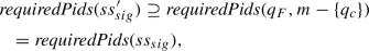
  by conditions 2 and 1, respectively. Hence

  

  But this implies

  

  which contradicts the definition of $ss_{sig}$. Hence $ss_{sig} \in SC$, as required.

• 2. Suppose $ss_{sig} \in SC$ and $\pi \in Sym(T)$. Then $\pi (ss_{sig}) \in C$ since C is closed under permutations. Further

  

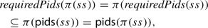
  using condition 3. Hence $\pi (ss_{sig}) \in SC$.

$\square$

In order to prove Proposition 36, we show that the conditions of Lemma 48 are satisfied. The following lemma deals with the easy cases.

Lemma 49

For each set $\mathcal {F}$ of chains of families, and for each system state $(q_F,m)$,  satisfies conditions 1–3 of Lemma 48.

The following lemma deals with condition 4 of Lemma 48.

Lemma 50

Suppose:

• 1. The system is closed;

• 2. For every reachable state $ss \in \mathcal {R}$, the required process identities correspond to references in ss:

  

Then condition 4 of Lemma 48 holds:

Note that the first premise is a premise of Proposition 36; the second premise holds automatically for the technique in Definition 33.

The final condition of Lemma 48 was a premise of Proposition 36. This completes the proof of Proposition 36.

References

Abdulla, P., Jonsson, B., Nilsson, M., d’Orso J.: Regular model checking made simple and efficient. In: Proceedings of CONCUR’02, 13th International Conference on Concurrency Theory, Volume 2421 of LNCS, pp. 116–130 (2002)
Abdulla, P., Jonsson, B., Nilsson, M., Saksena M.: A survey of regular model checking. In: Proceedings of Concur, volume 3170 of LNCS, pp. 35–48 (2004)
Abdulla, P., Jonsson, B., Nilsson, M., Saksena M.: General decidability theorems for infinite-state systems. In: Proceedings of the Symposium on Logic in Computer Science, pp. 313–321, 08 (1996)
Abdulla, Parosh, Haziza, Frédéric., Holík, Lukáš: Parameterized verification through view abstraction. Int. J. Softw. Tools Technol. Transfer 18, 495–516 (2016)
Abdulla, P.A., Jonsson, B., Trinh, C.Q.: Automated verification of linearization policies. In: Proceedings of SAS 2016, volume 9837 of LNCS, pp. 61–83. Springer (2016)
Abdulla, P.A., Jonsson, B., Trinh, C.Q.: Fragment abstraction for concurrent shape analysis. In: Proceedings of ESOP 2018, volume 10801 of LNCS, pp. 442–471. Springer (2018)
Abdullah, Parosh, Haziza, Frédéric., Holík, Lukáš, Jonsson, Bengt, Rezine, Ahmed: An integrated specification and verification technique for highly concurrent data structures. Int. J. Softw. Tools Technol. Transfer 19, 549–563 (2017)
Amit, D., Rinetzky, N., Reps, T., Sagiv, M., Yahav, E.: Comparison under abstraction for verifying linearizability. In: Computer Aided Verification, volume 4590 of LNCS, pp. 477–490. Springer (2007)
Apt, K.R., Kozen, D.C.: Limits for automatic verification of finite-state concurrent systems. Inf. Process. Lett. 22(6), 307–309 (1986)
Berdine, J., Lev-Ami, T., Manevich, R., Ramalingam, G., Sagiv, M.: Thread quantification for concurrent shape analysis. In: Proceedings of CAV 2008, volume 5123 of LNCS, pp. 399–413. Springer (2008)
Blondin, M., Finkel, A., Haase, C., Haddad, S.: Approaching the coverability problem continuously. In: Proceedings of TACAS 2016, volume 9636 of LNCS, pp. 480–496 (2016)
Bouajjani, A., Emmi, M., Enea, C., Hamza, J.: On reducing linearizability to state reachability. Inf. Comput. 261, 383–400 (2018)
Bouajjani, A., Habermehl, P., Vojnar, T.: Abstract regular model checking. In: Proceedings of International Conference on Computer Aided Verification, volume 3114 of LNCS, pp. 372–386, (2004)
Bouajjani, A., Jonsson, B., Nilsson, M., Touili, T.: Regular model checking. In: Proceedings of the 12th International Conference on Computer Aided Verification, volume 1855 of LNCS, pp. 403–418 (2000)
Bošnački, Dragan, Dams, Dennis, Holenderski, Leszek: Symmetric Spin. Int. J. Softw. Tools Technol. Transfer 4, 92–106 (2002)
Chakraborty, S., Henzinger, T.A., Sezgin, A., Sezgin, V.: Vafeiadis. Aspect-oriented linearizability proofs. Log. Methods Computer Sci. 11(1), (2015)
Clarke, E.M., Emerson, E.A., Jha, S., Sistla, A.P.: Symmetry reductions in model checking. In: Proceedings of the 10th International Conference on Computer-Aided Verification (CAV ’98), pp. 147–158 (1998)
Clarke, E.M., Enders, R., Filkorn, T., Jha, S.: Exploiting symmetry in temporal logic model checking. Formal Methods Syst. Des. 9, 77–104 (1996)
Clarke, E. M., Grumberg, O.: Avoiding the state explosion problem in temporal logic model checking. In: Proceedings of the 6th Annual Association for Computing Machinery Symposium on Principles of Distributed Computing, pp. 294–303 (1987)
Dams, D., Lakhnech, Y., Steffen, M.: Iterating transducers. J. Logic Algeb. Program. 52–53, 109–127 (2002)
Delzanno, G., Raskin, J.-F., Van Begin, L.: Attacking symbolic state explosion. In: Computer Aided Verification, pp. 298–310 (2001)
Dodds, M., Haas, A., Kirsch, C.: A scalable, correct time-stamped stack. In: Proceedings of POPL 2015, pp. 233–246. ACM (2015)
Emerson, E.A., Namjoshi, K.S.: Reasoning about rings. In: Proceedings of the Symposium on Principles of Programming Languages (POPL ’95) (1995)
Emerson, E.A., Sistla, A.P.: Symmetry and model checking. Formal Methods Syst. Des. 9, 105–131 (1996)
Esparza, J., Ledesma-Garza, R., Majumdar, R., Meyer, P., Niksic F.: An SMT-based approach to coverability analysis. In: Proceedings of CAV 2014, volume 8559 of LNCS, pp. 603–619 (2014)
Flanagan, C., Qadeer, S.: Thread-modular model checking. In: Proceedings of SPIN 2003, volume 2648 of LNCS, pp. 213–224 (2003)
German, S.M., Sistla, A.P.: Reasoning about systems with many processes. J. ACM 39(3), 675–735 (1992)
Gibson-Robinson, T., Armstrong, P., Boulgakov, A., Roscoe, A.W.: FDR3: a parallel refinement checker for CSP. Int. J. Softw. Tools Technol. Transf. (2015)
Gibson-Robinson, Thomas, Lowe, Gavin: Symmetry reduction in CSP model checking. Softw. Tools Technol. Transf. 21, 567–605 (2019)
Goldsmith, M., Moffat, N., Roscoe, B., Whitworth, T., Zakiuddin, I.: Watchdog transformations for property-oriented model checking. In: Proceedings of Formal Methods Europe (FME 2003), volume 2805 of LNCS, pp. 600–616 (2003)
Haziza, F., Holík, L., Meyer, R., Wolff, S.: Pointer race freedom. In Jobstmann, V., Rustan, K., Leino, M. (eds.), Verification, Model Checking, and Abstract Interpretation, pp. 393–412 (2016)
Hendler, D., Shavit, N., Yerushalmi L.: A scalable lock-free stack algorithm. In: Proceedings of the Sixteenth Annual ACM Symposium on Parallelism in Algorithms and Architectures, pp. 206–215 (2004)
Henzinger, T.A., Sezgin, A., Vafeiadis V.: Aspect-oriented linearization proofs. In: Proceedings of CONCUR 2013, volume 8052 of LNCS, pp. 242–256. Springer (2013)
Herlihy, M., Shavit, N.: The Art of Multiprocessor Programming. Morgan Kaufmann (2012)
Herlihy, M., Wing, J.M.: Linearizability: a correctness condition for concurrent objects. ACM Trans. Program. Lang. Syst. 12(3), 463–492 (1990)
Holík, L., Tomáš, V., Roland Meyer, A., Sebastian, W.: Effect summaries for thread-modular analysis. In: Proceedings of SAS 2017, volume 10422 of LNCS, pp. 169–191. Springer (2017)
Ip, C.N., Dill, D.L.: Better verification through symmetry. Formal Methods Syst. Des. 9, 41–75 (1996)
Kaiser, A., Kroening, D., Wahl, T.: A widening approach to multithreaded program verification. ACM Trans. Program. Lang. Syst. 36(4), 1–29 (2014)
Kesten, Y., Maler, O., Marcus, M., Pnueli, A., Shahar E.: Symbolic model checking with rich assertional languages. Theoretical Computer Science, pp. 93–112 (2001)
Lowe, G.: View abstraction for systems with component identities. In: Proceedings of the International Symposium on Formal Methods (FM 2018), volume 10951 of LNCS, pp. 502–522. Springer (2018)
Lowe, G.: Discovering and correcting a deadlock in a channel implementation. Formal Aspects Comput. 31, 411–419 (2019)
Lubachevsky, B.: An approach to automating the verification of compact parallel coordination programs. Acta Informatica 21(2), 125–169 (1984)
Manevich, R., Yahav, E., Ramalingam, G., Sagiv, M.: Predicate abstraction and canonical abstraction for singly-linked lists. In: Proceedings of VMCAI 2005, volume 3385 of LNCS, pp. 181–198. Springer (2005)
Mazur, T., Lowe, G.: CSP-based counter abstraction for systems with node identifiers. Sci. Comput. Program. 81, 3–52 (2014)
Meyer, R., Sebastian, W.: Decoupling lock-free data structures from memory reclamation for static analysis. In: Proceedings of the ACM on Programming Languages, 3(POPL) (2019)
Michael, M., Michael, S.: Simple, fast, and practical non-blocking and blocking concurrent queue algorithms. In: Proceedings of the Fifteenth Annual ACM Symposium on Principles of Distributed Computing, pp. 267–275 (1996)
Moffat, N., Goldsmith, M., Roscoe. B.: A representative function approach to symmetry exploitation for csp refinement checking. In: Liu, S., Maibaum, T., Araki, K. (eds.), Formal Methods and Software Engineering, pp. 258–277, Berlin, Heidelberg (2008)
Oracle. LockSupport (Java SE9 & JDK 9). https://docs.oracle.com/javase/9/docs/api/java/util/concurrent/locks/LockSupport.html
Pnueli, A., Xu, J., Zuck L.D.: Liveness with (0, 1, \(\infty \))-counter abstraction. In: CAV’02: Proceedings of the 14th International Conference on Computer Aided Verification, pp. 107–122 (2002)
Roscoe, A.W.: Understanding Concurrent Systems. Springer (2010)
Roscoe, A.W., Creese, S.J.: Data independent induction over structured networks. In: Proceedings of PDPTA2000 (2000)
Sagiv, M., Reps, T., Wilhelm, R.: Parametric shape analysis via 3-valued logic. Trans. Program. Lang. Syst. (2002)
Sistla, A.P., Gyuris, V., Emerson, E.A.: SMC: A symmetry-based model checker for verification of safety and linveness properties. ACM Trans. Softw. Eng. Methodol. 9(2), 133–166 (2000)
Sufrin, B..: Communicating Scala Objects. In: Proceedings of Communicating Process Architectures (CPA) (2008)
Touili, T.: Regular model checking using widening techniques. In: Electronic Notes in Theoretical Computer Science, 50(4), Proceedings of VEPAS’01 (2001)
Treiber, R.K.: Systems programming: Coping with parallelism. Technical Report RJ 5118, IBM (1986)
Vardi, M.Y., Wolper, P.: An automata-theoretic approach to automatic program verification. In: Proceedings of LICS’86, pp. 332–344 (1986)
Wolper, P., Boigelot, B.: Verifying systems with infinite but regular state spaces. In: Proceedings of 10th International Conference on Computer Aided Verification, volume 1427 of LNCS (1998)
Wolper, P., Lovinfosse, V.: Verifying properties of large sets of processes with network invariants. In: Automatic Verification Methods for Finite State Systems, volume 407 of LNCS, pp. 68–80 (1989)
Wolper, P.: Expressing interesting properties of programs in propositional temporal logic. In: Thirteenth Annual ACM Symposium on Principles of Programming Languages, pp. 184–193 (1986)
Acknowledgements
I would like to thank Tom Gibson-Robinson for useful discussions concerning this work, and for extending the FDR4 API to support various functions necessary for the implementation. I would also like to thank the anonymous referees for their useful comments and suggestions.
Author information
Authors and Affiliations
Corresponding author
Additional information
Publisher's Note
Springer Nature remains neutral with regard to jurisdictional claims in published maps and institutional affiliations.