A new method based on Taylor expansion and nearest-node strategy to impose Dirichlet and Neumann boundary conditions in ordinary state-based Peridynamics

Abstract

Peridynamics is a non-local continuum theory which is able to model discontinuities in the displacement field, such as crack initiation and propagation in solid bodies. However, the non-local nature of the theory generates an undesired stiffness fluctuation near the boundary of the bodies, phenomenon known as “surface effect”. Moreover, a standard method to impose the boundary conditions in a non-local model is not currently available. We analyze the entity of the surface effect in ordinary state-based peridynamics by employing an innovative numerical algorithm to compute the peridynamic stress tensor. In order to mitigate the surface effect and impose Dirichlet and Neumann boundary conditions in a peridynamic way, we introduce a layer of fictitious nodes around the body, the displacements of which are determined by multiple Taylor series expansions based on the nearest-node strategy. Several numerical examples are presented to demonstrate the effectiveness and accuracy of the proposed method.

1 Introduction

The propagation of cracks in solids and structures is one of the most common problems in structural engineering. In recent years, a new non-local continuum theory able to simulate crack propagation, named peridynamic theory, attracted the attention of many researchers. Each point in a body modelled with peridynamics interacts with all the neighboring points within a distance $\delta$. The non-locality of the peridynamic theory is essential to describe fracture phenomena in solid bodies without ad hoc criteria. Firstly, the so-called “bond-based peridynamics” was developed [40], which however has a limited capability of prescribing the Poisson’s ratio. This shortcoming is avoided by the second formulation of the theory, named “state-based peridynamics” [42].

The non-local nature of the theory leads to two interrelated problems near the boundary of the body: the “surface effect” and the difficulty to impose the boundary conditions [9]. The surface effect, sometimes also called “skin effect”, is due to the fact that peridynamic points near the boundary lack some neighboring points, leading to an undesired variation of the stiffness properties in the most external layer of the body [16, 19]. Bond-based and state-based peridynamic models exhibit respectively a softening and a hardening-softening behavior near the boundary [2, 20, 35].

Imposing boundary conditions in a peridynamic model is not a trivial task to accomplish. The application of the boundary conditions to the points on the boundary, as one would do in a local model, leads to large fluctuations of the solution near the boundary [16]. In [21] it is suggested that external loads and constraints should be imposed on a layer of finite thickness respectively inside and outside the body. This strategy is surely closer to a non-local concept, but it is not really clear the proper procedure to “distribute” the boundary conditions over the finite layers. In the following, we present some of the most commonly used methods to mitigate the surface effect and impose the boundary conditions in a peridynamic model.

A possible approach is to couple peridynamics with classical continuum mechanics: peridynamics is employed only in the interior of the body and the layer of material near the boundary is modelled, for instance, with the Finite Element Method [11, 25, 38, 45, 47, 48], with the Carrera Unified Formulation [30], with the Extended Finite Element Method [13, 14] or with the Meshless Local Exponential Basis Functions method [39]. In this way, the surface effect and the problem of the imposition of the boundary conditions in peridynamics is avoided. However, if cracks initiate or propagate near the boundary, those regions must inevitably be modelled with peridynamics and the coupling approach is not suitable to avoid the boundary issues. Furthermore, there are some spurious effects at the interface of the coupling region due to the different formulations of peridynamics and classical continuum mechanics (see the computation of out-of-balance forces in [26]).

The maximum distance of interaction, namely $\delta$, is a measure of the non-locality of the theory. Therefore, the external layer of the body which is affected by the surface effect is thinner as $\delta$ approaches 0. Similarly, the imposition of the boundary conditions in a local way (constraints and loads applied only to the points closest to the boundary) becomes a better approximation if $\delta$ tends to 0. Since the number of nodes is bound to increase as $\delta$ decreases, the computational effort may become excessive. In this case, the variable horizon method can be employed to decrease the value of $\delta$ near the boundaries [2, 3, 6, 31,32,33, 44]. However, this approach of reducing the non-local nature of the peridynamic theory is solely capable of confining the solution fluctuation in a smaller region, but never of completely correcting it.

The approach of modifying the stiffness properties of the bonds near the boundary has been proposed in many methods: the force normalization method [20], the force density method [15], the energy method [21, 27], the volume method [1] and the position-aware linear solid constitutive model [23]. The comparison of these methods, carried out in [16], highlights that there are still some residual fluctuations of the solution near the boundary because they do not cope with the problem of the imposition of the boundary conditions in a non-local way. Another recently devised approach consists in modifying the peridynamic formulation in points which are affected by the surface effect in order to recover the classical mechanics solution for $\delta \rightarrow 0$ [4, 46]. Nevertheless, the treatment of the boundaries becomes much more complex.

The method of the “fictitious nodes” consists in adding around the body some nodes which provide the previously lacking interactions near the boundary, mitigating in this way the surface effect [12, 15, 34]. The fictitious nodes have been employed also to impose the boundary conditions: the displacements of the fictitious nodes are extrapolated by means of various types of functions, such as constant, linear, polynomial, sinusoidal or odd functions, in order to obtain the desired value of the constraint or load [6,7,8, 16, 21, 22, 28, 29, 31, 49]. Moreover, the displacements of the fictitious nodes can be determined also by means of the formulae of classical continuum mechanics to enforce the desired load at the boundary [16, 22, 28, 31, 49]. However, these procedures to impose the boundary conditions are case-dependent and are applicable only for simple geometries and boundary conditions.

We proposed a new version of the “Taylor-based extrapolation method” adopting the nearest-node strategy [35]: the displacements of the fictitious nodes are determined as functions of the displacements of their closest real nodes by means of multiple Taylor series expansions truncated at a general order $n_{max}$. The surface effect is sensibly reduced by this effective method. Moreover, the boundary of the body is discretized by a new type of nodes, named “boundary nodes”. As the fictitious nodes, the boundary nodes do not constitute new degrees of freedom in the model because their displacements are determined by means of the Taylor-based extrapolation method. Dirichlet boundary conditions are included in the Taylor series expansion of the displacements of the boundary nodes about their closest real nodes, whereas Neumann boundary conditions are imposed through the peridynamic concept of force flux.

The paper is organized as follows: Sect. 2 presents a brief review of the ordinary state-based peridynamic theory, particularly focusing on the peridynamic stress tensor, the force flux, the surface effect and the imposition of boundary conditions; Sect. 3 illustrates the Taylor-based extrapolation method and the imposition of boundary conditions in a peridynamic model; Sect. 4 shows the discretization of the peridynamic model, the numerical evaluation of the peridynamic stress tensor and of the force flux, and the numerical implementation of the proposed method; Sect. 5 compares the numerical results of several meaningful 2-dimensional examples obtained without any corrections at the boundary and by using the proposed method; Sect. 6 shows the differences that may arise in crack propagation near the boundaries between corrected and uncorrected models; Sect. 7 draws the conclusions.

2 Review of peridynamic theory

Peridynamic points interact with each other, even within finite distance, through entities named “bonds”. A bond is identified by the relative position vector in the reference configuration as

$$\begin{aligned} \varvec{\xi } = {\textbf{x}}' - {\textbf{x}} \, , \end{aligned}$$

(1)

where ${\textbf{x}}$ and ${\textbf{x}}'$ are the position vectors of two points in a body $\mathcal {B}$ modelled with peridynamics. The bond vanishes if the distance between the interacting points exceeds the value $\delta$, called “horizon”. A point ${\textbf{x}}$ therefore interacts with all the points ${\textbf{x}}'$ inside its neighborhood, which is defined as

$$\begin{aligned} \mathcal {H}_{{\textbf{x}}} = \big \{ \, {\textbf{x}}' \in \mathcal {B}_r: \Vert \varvec{\xi }\Vert \le \delta \, \big \} \, , \end{aligned}$$

(2)

where $\mathcal {B}_r$ is the body in the reference configuration. Point ${\textbf{x}}$ is named “source point” and the points within $\mathcal {H}_{{\textbf{x}}}$ are named “family points”.

In the deformed body configuration $\mathcal {B}_d$ at time t, the relative displacement vector $\varvec{\eta }$ is defined as

$$\begin{aligned} \varvec{\eta } = {\textbf{u}}({\textbf{x}}',t) - {\textbf{u}}({\textbf{x}},t) \, , \end{aligned}$$

(3)

where ${\textbf{u}}$ is the displacement field. Note that $\varvec{\xi } + \varvec{\eta }$ is the relative position of points ${\textbf{x}}$ and ${\textbf{x}}'$ in the deformed configuration.

The peridynamic equation of motion of a point ${\textbf{x}}$ within the body $\mathcal {B}$ is given by [40, 42]:

$$\begin{aligned} \rho ({\textbf{x}}) \, \ddot{{\textbf{u}}}({\textbf{x}},t) = \int _{\mathcal {H}_{{\textbf{x}}}} {\textbf{f}}({\textbf{x}},{\textbf{x}}',t) \mathop {}\! \textrm{d} {V}_{{\textbf{x}}'} + {\textbf{b}}({\textbf{x}},t) \, , \end{aligned}$$

(4)

where $\rho$ is the material density, $\ddot{{\textbf{u}}}$ is the acceleration field, ${\textbf{f}}$ is the pairwise force density, $\mathop {}\! \textrm{d} {V}_{{\textbf{x}}'}$ is the differential volume of a point ${\textbf{x}}'$ within the neighborhood $\mathcal {H}_{{\textbf{x}}}$ and ${\textbf{b}}$ is the external force density field. The pairwise force density represents the force (per unit volume squared) in a bond.

Fig. 1

Body modelled with ordinary state-based peridynamics in the reference configuration $\mathcal {B}_r$ and deformed configuration $\mathcal {B}_d$: a pairwise force density ${\textbf{f}}$ arises in the bond $\varvec{\xi }$ due to the deformation of the body

The peridynamic equilibrium equation is derived from Eq. 4 by dropping the dependence on time:

$$\begin{aligned} - \int _{\mathcal {H}_{{\textbf{x}}}} {\textbf{f}}({\textbf{x}},{\textbf{x}}') \mathop {}\! \textrm{d} {V}_{{\textbf{x}}'} = {\textbf{b}}_{{\textbf{x}}} \, . \end{aligned}$$

(5)

where ${\textbf{b}}_{{\textbf{x}}} = {\textbf{b}} ({\textbf{x}})$. ${\textbf{f}}({\textbf{x}},{\textbf{x}}')$ is the force density applied to point ${\textbf{x}}$ due to the interaction with a point ${\textbf{x}}'$ inside its neighborhood. Conversely, point ${\textbf{x}}$ belongs to the neighborhood $\mathcal {H}_{{\textbf{x}}'}$, thus a force density ${\textbf{f}}({\textbf{x}}',{\textbf{x}}) = -{\textbf{f}}({\textbf{x}},{\textbf{x}}')$ is applied to point ${\textbf{x}}'$ (see Fig. 1). The formulae to compute the pairwise force density depending on the deformation of the body are shown in the following section.

2.1 Ordinary state-based peridynamics

In state-based peridynamics, the pairwise force density is defined as [42]

$$\begin{aligned} {\textbf{f}}({\textbf{x}},{\textbf{x}}') = \underline{{\textbf{T}}} [{\textbf{x}}] \langle \varvec{\xi } \rangle - \underline{{\textbf{T}}} [{\textbf{x}}'] \langle -\varvec{\xi } \rangle \, , \end{aligned}$$

(6)

where $\underline{{\textbf{T}}}$ is the force density vector state. $\underline{{\textbf{T}}} [{\textbf{x}}] \langle \varvec{\xi } \rangle$ and $\underline{{\textbf{T}}} [{\textbf{x}}'] \langle -\varvec{\xi } \rangle$ depend respectively on points ${\textbf{x}}$ and ${\textbf{x}}'$, and they respectively operate on bonds $\varvec{\xi }$ and $-\varvec{\xi }$.

In an ordinary peridynamic material, the force density vector state is aligned with the corresponding bond for any deformation, as depicted in Fig. 1, and it can be written as

$$\begin{aligned} \underline{{\textbf{T}}} [{\textbf{x}}] \langle \varvec{\xi } \rangle = \underline{t} [{\textbf{x}}] \langle \varvec{\xi } \rangle \, \, \underline{{\textbf{M}}} \langle \varvec{\xi } \rangle \, , \end{aligned}$$

(7)

where $\underline{t}$ is the force density scalar state (magnitude of $\underline{{\textbf{T}}}$) and $\underline{{\textbf{M}}}$ is the deformed direction vector state (unit vector in the direction of $\underline{{\textbf{T}}}$), defined as

$$\begin{aligned} \underline{{\textbf{M}}} \langle \varvec{\xi } \rangle = \frac{\varvec{\xi } + \varvec{\eta }}{\Vert \varvec{\xi } + \varvec{\eta } \Vert } \, . \end{aligned}$$

(8)

Note that $\underline{{\textbf{M}}} \langle \varvec{\xi } \rangle = -\underline{{\textbf{M}}} \langle -\varvec{\xi } \rangle$.

Furthermore, under the assumption of small deformation ($\varvec{\eta } \ll \varvec{\xi }$), the deformed direction vector state can be approximated with the bond direction unit vector in the reference configuration:

$$\begin{aligned} {\textbf{m}} = \frac{\varvec{\xi }}{\Vert \varvec{\xi } \Vert } \, . \end{aligned}$$

(9)

Therefore, the pairwise force density can be rewritten as

$$\begin{aligned} {\textbf{f}}({\textbf{x}},{\textbf{x}}') = \big ( \, \underline{t} [{\textbf{x}}] \langle \varvec{\xi } \rangle + \underline{t} [{\textbf{x}}'] \langle -\varvec{\xi } \rangle \, \big ) \, {\textbf{m}} \, . \end{aligned}$$

(10)

The reference position scalar state $\underline{x}$, representing the bond length in the reference configuration, and the extension scalar state $\underline{e}$, describing the elongation (or contraction) of the bond in the deformed body configuration, are respectively defined as

$$\begin{aligned} \underline{x}= & {} \Vert \varvec{\xi } \Vert \, , \end{aligned}$$

(11)

$$\begin{aligned} \underline{e}= & {} \Vert \varvec{\xi } + \varvec{\eta } \Vert - \Vert \varvec{\xi } \Vert \, . \end{aligned}$$

(12)

The influence of the neighborhood $\mathcal {H}_{{\textbf{x}}}$ on a source point ${\textbf{x}}$ is expressed by two non-local properties of that point, the weighted volume m and the dilatation $\theta$, which are defined as

$$\begin{aligned} m_{{\textbf{x}}}= & {} \int _{\mathcal {H}_{{\textbf{x}}}} \underline{\omega } \, \underline{x}^2 \mathop {}\! \textrm{d} {V}_{{\textbf{x}}'} \, , \end{aligned}$$

(13)

$$\begin{aligned} \theta _{{\textbf{x}}}= & {} \frac{c_{\theta }}{m_{{\textbf{x}}}} \int _{\mathcal {H}_{{\textbf{x}}}} \underline{\omega } \, \underline{x} \, \underline{e} \mathop {}\! \textrm{d} {V}_{{\textbf{x}}'} \, , \end{aligned}$$

(14)

where $\underline{\omega }$ is a prescribed spherical influence function and $c_{\theta }$ is a peridynamic constant. We adopt the Gaussian influence function

$$\begin{aligned} \underline{\omega } = e^{ -\frac{\Vert \varvec{\xi } \Vert ^2}{\delta ^2} } \, , \end{aligned}$$

(15)

since it assures a smooth convergence of the numerical integration [36].

The weighted volume describes the “fullness” of the neighborhood: a neighborhood completely full of peridynamic points results in the maximum value of m, whereas the weighted volume of an incomplete neighborhood has a lower value. This lack of neighboring points is the origin of stiffness fluctuations, the so-called “surface effect” [16], near the boundary of the body. The surface effect is further analyzed in Sect. 2.4.

On the other hand, the dilatation represents the volumetric deformation of the neighborhood. Consider a point ${\textbf{x}}$ subjected to a homogeneous, isotropic and small deformation $\overline{\varepsilon }$, so that $\underline{e} = \overline{\varepsilon } \, \underline{x}$ for each bond. The peridynamic dilatation $\theta$ of point ${\textbf{x}}$ corresponds to the dilatation $\theta _{cl}$ in classical continuum mechanics under the same deformation if the constant $c_{\theta }$ is chosen as [17, 35, 42]

$$\begin{aligned} c_{\theta } = {\left\{ \begin{array}{ll} 3 &{} \text {in 3D,} \\ 2 &{} \text {in 2D plane strain,} \\ \frac{2 (1-2\nu )}{1-\nu } &{} \text {in 2D plane stress,} \\ 1-2\nu &{} \text {in 1D axial loading,} \\ \end{array}\right. } \end{aligned}$$

(16)

where $\nu$ is the Poisson’s ratio.

The force density scalar state can be computed as [35]

$$\begin{aligned} \underline{t} [{\textbf{x}}] \langle \varvec{\xi } \rangle = k_{\theta } \, \frac{\underline{\omega } \, \underline{x}}{m_{{\textbf{x}}}} \, \theta _{{\textbf{x}}} + k_e \, \frac{\underline{\omega } \, \underline{e}}{m_{{\textbf{x}}}} \, . \end{aligned}$$

(17)

where $k_{\theta }$ and $k_e$ are the peridynamic stiffness constants. These constants are derived by equalizing the peridynamic strain energy density in a point ${\textbf{x}}$ with a complete neighborhood under homogeneous deformation, with the classical continuum mechanics strain energy density in a point subjected to the same deformation [17, 35, 42]:

$$\begin{aligned} k_{\theta }= & {} {\left\{ \begin{array}{ll} \frac{-3(1-4\nu )}{2(1+\nu )(1-2\nu )} \, E &{} \text {in 3D,} \\ \frac{-(1-4\nu )}{(1+\nu )(1-2\nu )} \, E &{} \text {in 2D plane strain,} \\ \frac{-(1-3\nu )}{(1+\nu )(1-2\nu )} \, E &{} \text {in 2D plane stress,} \\ \frac{\nu }{(1+\nu )(1-2\nu )} \, E &{} \text {in 1D axial loading,} \\ \end{array}\right. } \end{aligned}$$

(18)

$$\begin{aligned} k_{e}= & {} {\left\{ \begin{array}{ll} \frac{15}{2(1+\nu )} \, E &{} \text {in 3D,} \\ \frac{4}{1+\nu } \, E &{} \text {in 2D plane strain or plane stress,} \\ \frac{1}{1+\nu } \, E &{} \text {in 1D axial loading,} \\ \end{array}\right. } \end{aligned}$$

(19)

where E is the Young’s modulus.

By substituting Eq. 17 in Eq. 10, the pairwise force density is computed as

$$\begin{aligned} {\textbf{f}}({\textbf{x}},{\textbf{x}}') {=} \left[ k_{\theta } \left( \frac{\theta _{{\textbf{x}}}}{m_{{\textbf{x}}}} {+} \frac{\theta _{{\textbf{x}}'}}{m_{{\textbf{x}}'}} \right) \underline{\omega } \, \underline{x} {+} k_e \left( \frac{1}{m_{{\textbf{x}}}} {+} \frac{1}{m_{{\textbf{x}}'}} \right) \underline{\omega } \, \underline{e} \right] {\textbf{m}} \, . \nonumber \\ \end{aligned}$$

(20)

Note that the magnitude of the pairwise force density in ordinary state-based peridynamics depends on the neighborhood properties (m and $\theta$) of the two points ${\textbf{x}}$ and ${\textbf{x}}'$ connected by the bond. Hence, the resultant of all the bond forces in a point ${\textbf{x}}$, obtained with the integral of the peridynamic equilibrium equation (Eq. 5), depends on the deformation of the points within a $2\delta$-distance from ${\textbf{x}}$.

2.2 Peridynamic stress tensor

The peridynamic stress tensor, introduced in [18], is defined in a point ${\textbf{x}}$ with a complete neighborhood as

$$\begin{aligned} \varvec{\tau }_{{\textbf{x}}} ={} & {} \frac{1}{2} \int _{\varOmega } \int _{0}^{\delta } \int _{s}^{\delta } {\textbf{f}} ({\textbf{x}}-s{\textbf{m}}, {\textbf{x}}+(r-s){\textbf{m}}) \nonumber \\ {}{} & {} \otimes {\textbf{m}} \, r^2 \mathop {}\! \textrm{d} {r} \mathop {}\! \textrm{d} {s} \mathop {}\! \textrm{d} {\varOmega }_{{\textbf{m}}} \, , \end{aligned}$$

(21)

where $\varOmega$ is a unit sphere centered in ${\textbf{x}}$ and $\mathop {}\! \textrm{d} {\varOmega }_{{\textbf{m}}}$ is the differential solid angle on $\varOmega$ in any bond direction ${\textbf{m}}$. The points ${\textbf{x}}-s{\textbf{m}}$ and ${\textbf{x}}+(r-s){\textbf{m}}$ are connected by a bond passing through point ${\textbf{x}}$, and we respectively name them ${\textbf{x}}'$ and ${\textbf{x}}''$. Therefore, $s = \Vert {\textbf{x}}' - {\textbf{x}} \Vert$ and $r = \Vert {\textbf{x}}'' - {\textbf{x}}' \Vert$, as shown in Fig. 2. s is the distance between points ${\textbf{x}}$ and ${\textbf{x}}'$, whereas r is the length of the bond between ${\textbf{x}}'$ and ${\textbf{x}}''$. The definition of the integration domain allows to take into account all the bonds passing through point ${\textbf{x}}$. Note that each bond passing through ${\textbf{x}}$ (between ${\textbf{x}}'$ and ${\textbf{x}}''$) has a corresponding bond in the opposite direction (between ${\textbf{x}}''$ and ${\textbf{x}}'$), so that the same pairwise force density is integrated twice in Eq. 21. This is the reason why the factor 1/2 appears at the beginning of the formula.

Fig. 2

Main variables involved in the computation of the peridynamic stress tensor in point ${\textbf{x}}$: the bond direction ${\textbf{m}}$ lies on the unit sphere $\varOmega$ (dotted line); point ${\textbf{x}}'$ lies on the opposite direction of ${\textbf{m}}$ at a distance s from ${\textbf{x}}$, with $0< s < \delta$ (dashed line); point ${\textbf{x}}''$ lies on the direction ${\textbf{m}}$ at a distance r from ${\textbf{x}}'$, with $s< r < \delta$ (dashdotted line)

The integral over the unit sphere $\varOmega$ is not affected by the variables s and r, but it depends only on the bond direction ${\textbf{m}}$. On the other hand, the integrals related to $\mathop {}\! \textrm{d} {s}$ and $\mathop {}\! \textrm{d} {r}$ are interdependent, as shown by the integration domain depicted in Fig. 3. For later use, the peridynamic stress tensor in a point ${\textbf{x}}$ with a complete neighborhood is rewritten by changing the order of the integrals:

$$\begin{aligned} \begin{aligned} \varvec{\tau }_{{\textbf{x}}}&= \frac{1}{2} \int _{\varOmega } \int _{0}^{\delta } \int _{0}^{r} {\textbf{f}} ({\textbf{x}}', {\textbf{x}}'') \otimes {\textbf{m}} \, r^2 \mathop {}\! \textrm{d} {s} \mathop {}\! \textrm{d} {r} \mathop {}\! \textrm{d} {\varOmega }_{{\textbf{m}}} \\&= \frac{1}{2} \int _{\mathcal {H}_{{\textbf{x}}}} \int _{0}^{r} {\textbf{f}} ({\textbf{x}}', {\textbf{x}}'') \otimes {\textbf{m}} \, \mathop {}\! \textrm{d} {s} \mathop {}\! \textrm{d} {V}_{{\textbf{x}}''} \, , \end{aligned} \end{aligned}$$

(22)

where $\mathop {}\! \textrm{d} {V}_{{\textbf{x}}''} = r^2 \mathop {}\! \textrm{d} {r} \mathop {}\! \textrm{d} {\varOmega }_{{\textbf{m}}}$.

Fig. 3

Integration domain for the computation of the peridynamic stress tensor for a fixed bond direction: for any value of s in the interval $]0,\delta [$, r lies in the interval $]s,\delta [$ (see limits of integration in Eq. 21); for any value of r in the interval $]0,\delta [$, s lies in the interval ]0, r[ (see limits of integration in Eq. 22)

Under the assumption of homogeneous deformation, the bonds with the same length and direction have the same pairwise force density in any position of the body. This means that, for each bond of length r and direction ${\textbf{m}}$, its pairwise force density does not depend on s anymore. Therefore, $\varvec{\tau }_{{\textbf{x}}}$ can be simplified from Eq. 22 as follows:

$$\begin{aligned} \begin{aligned} \varvec{\tau }_{{\textbf{x}}}&= \frac{1}{2} \int _{\mathcal {H}_{{\textbf{x}}}} \left( \int _{0}^{r} \mathop {}\! \textrm{d} {s} \right) {\textbf{f}} ({\textbf{x}}, {\textbf{x}}'') \otimes {\textbf{m}} \mathop {}\! \textrm{d} {V}_{{\textbf{x}}''} \\&= \frac{1}{2} \int _{\mathcal {H}_{{\textbf{x}}}} r \, {\textbf{f}} ({\textbf{x}}, {\textbf{x}}'') \otimes {\textbf{m}} \mathop {}\! \textrm{d} {V}_{{\textbf{x}}''} \, . \end{aligned} \end{aligned}$$

(23)

Note that, since the value of s does not affect ${\textbf{f}} ({\textbf{x}}', {\textbf{x}}'')$ in a body under homogeneous deformation, we conveniently choose the pairwise force density for $s=0$, i.e., ${\textbf{f}} ({\textbf{x}}, {\textbf{x}}'')$.

We want to compare the peridynamic stress tensor with the stress tensor in classical continuum mechanics for the same deformation conditions. For simplicity sake, we choose the 2-dimensional plane stress peridynamic model for a body subjected to two different conditions of homogeneous and small deformation: isotropic deformation, indicated by the superscript iso, and simple shear deformation, indicated by the superscript sh. Under those conditions, the strain and stress tensors in a point ${\textbf{x}}$ are given in classical continuum mechanics as

$$\begin{aligned}{} & {} \begin{aligned}&\quad \varvec{\varepsilon }_{{\textbf{x}}}^{\, iso} = \overline{\varepsilon }^{\, iso} \begin{bmatrix} 1 &{} 0 \\ 0 &{} 1 \end{bmatrix} \\&\quad \Rightarrow \quad \varvec{\sigma }_{{\textbf{x}}}^{\, iso} = \frac{E}{1-\nu } \, \overline{\varepsilon }^{\, iso} \begin{bmatrix} 1 &{} 0 \\ 0 &{} 1 \end{bmatrix} = \overline{\sigma }^{\, iso} \begin{bmatrix} 1 &{} 0 \\ 0 &{} 1 \end{bmatrix} \, , \end{aligned} \end{aligned}$$

(24)

$$\begin{aligned}{} & {} \begin{aligned}&\quad \varvec{\varepsilon }_{{\textbf{x}}}^{\, sh} = \overline{\varepsilon }^{\, sh} \begin{bmatrix} 0 &{} 1 \\ 1 &{} 0 \end{bmatrix} \\&\quad \Rightarrow \quad \varvec{\sigma }_{{\textbf{x}}}^{\, sh} = \frac{E}{1+\nu } \, \overline{\varepsilon }^{\, sh} \begin{bmatrix} 0 &{} 1 \\ 1 &{} 0 \end{bmatrix} = \overline{\sigma }^{\, sh} \begin{bmatrix} 0 &{} 1 \\ 1 &{} 0 \end{bmatrix} \, , \end{aligned} \end{aligned}$$

(25)

where $\overline{\varepsilon }^{\, iso}$ and $\overline{\varepsilon }^{\, sh}$ are the values of the imposed deformations and $\overline{\sigma }^{\, iso}$ and $\overline{\sigma }^{\, sh}$ are the corresponding stresses.

In the following analysis of the peridynamic stress tensor, only points with complete neighborhoods are considered. The inclination of a bond with respect to the x-axis is called $\phi$. Therefore, the bond direction in a 2-dimensional model can be written as ${\textbf{m}} = \{ \cos \phi , \, \sin \phi \}^{\top }$. Furthermore, the weighted volume of a point ${\textbf{x}}$ with a complete neighborhood is given from Eq. 13 by

$$\begin{aligned} \begin{aligned} m_{{\textbf{x}}}&= \int _{0}^{2 \pi } \int _{0}^{\delta } \Vert \varvec{\xi } \Vert ^3 \, e^{-\frac{\Vert \varvec{\xi } \Vert ^2}{\delta ^2}} \, h \mathop {}\! \textrm{d} {\xi }\mathop {}\! \textrm{d} {\phi }\\&= \frac{\pi ( e-2 )}{e} \, h \delta ^4 \, , \end{aligned} \end{aligned}$$

(26)

where h is the thickness of the 2-dimensional body.

In the case of a body subjected to a small isotropic deformation, any extension scalar state is $\underline{e}^{\, iso} = \overline{\varepsilon }^{\, iso} \underline{x}$ and the corresponding dilatation in a point ${\textbf{x}}$ with a complete neighborhood is $\theta _{{\textbf{x}}}^{\, iso} = c_{\theta } \, \overline{\varepsilon }^{\, iso}$. The peridynamic stress tensor under this condition is given from Eq. 23 as

$$\begin{aligned} \begin{aligned} \varvec{\tau }_{{\textbf{x}}}^{\, iso}&= \frac{1}{2} \int _{0}^{2 \pi } \int _{0}^{\delta } (c_{\theta } k_{\theta } + k_e ) \, \overline{\varepsilon }^{\, iso} \frac{2}{m_{{\textbf{x}}}} r^2 e^{-\frac{r^2}{\delta ^2}} \, \cdot \\&\quad \cdot \begin{Bmatrix} \cos \phi \\ \sin \phi \end{Bmatrix} \otimes \begin{Bmatrix} \cos \phi \\ \sin \phi \end{Bmatrix} h \, r \mathop {}\! \textrm{d} {r} \mathop {}\! \textrm{d} {\phi }\\&= \frac{E}{1-\nu } \, \overline{\varepsilon }^{\, iso} \frac{2 e \, h}{\pi (e-2) h \delta ^4} \int _{0}^{\delta } r^3 e^{-\frac{r^2}{\delta ^2}} \mathop {}\! \textrm{d} {r} \, \cdot \\&\quad \cdot \int _{0}^{2 \pi } \begin{bmatrix} \cos ^2 \phi &{} \cos \phi \sin \phi \\ \cos \phi \sin \phi &{} \sin ^2 \phi \end{bmatrix} \mathop {}\! \textrm{d} {\phi }\\&= \frac{E}{1-\nu } \, \overline{\varepsilon }^{\, iso} \frac{2 e}{\pi (e-2) \delta ^4} \cdot \frac{(e-2) \delta ^4}{2e} \begin{bmatrix} \pi &{} 0 \\ 0 &{} \pi \end{bmatrix} \\&= \frac{E}{1-\nu } \, \overline{\varepsilon }^{\, iso} \begin{bmatrix} 1 &{} 0 \\ 0 &{} 1 \end{bmatrix} \, . \end{aligned} \end{aligned}$$

(27)

The obtained peridynamic stress tensor yields the same result of the stress tensor computed with classical continuum mechanics in a point under isotropic deformation. Note that only a tensile stress $\tau _{11} = \tau _{22} = \overline{\sigma }^{\, iso}$ arises from the imposed deformation $\overline{\varepsilon }^{\, iso}$ and there is no shear stress ($\tau _{12} = 0$).

In the case of a body subjected to a small shear deformation $\overline{\varepsilon }^{\, sh}$, the extension scalar state can be computed by substituting $\varvec{\xi } = \{ \Vert \varvec{\xi } \Vert \cos \phi , \, \Vert \varvec{\xi } \Vert \sin \phi \}^{\top }$ and $\varvec{\eta } = \{ \overline{\varepsilon }^{\, sh} \Vert \varvec{\xi } \Vert \sin \phi , \, \overline{\varepsilon }^{\, sh} \Vert \varvec{\xi } \Vert \cos \phi \}^{\top }$ in Eq. 12:

$$\begin{aligned} \begin{aligned} \underline{e}^{\, sh}&= \sqrt{ \left[ \Vert \varvec{\xi } \Vert (\cos \phi + \overline{\varepsilon }^{\, sh} \sin \phi ) \right] ^2 + \left[ \Vert \varvec{\xi } \Vert (\sin \phi + \overline{\varepsilon }^{\, sh} \cos \phi ) \right] ^2} \\&\qquad - \Vert \varvec{\xi } \Vert \\&= \Vert \varvec{\xi } \Vert \sqrt{ 1 + 4 \, \overline{\varepsilon }^{\, sh} \cos \phi \sin \phi } - \Vert \varvec{\xi } \Vert \\&= 2 \, \overline{\varepsilon }^{\, sh} \Vert \varvec{\xi } \Vert \cos \phi \sin \phi \end{aligned} \end{aligned}$$

(28)

where the formula is simplified under the assumption of sufficiently small deformation by dropping the second order terms and employing the Taylor series expansion for the square root. The corresponding dilatation in a point ${\textbf{x}}$ with a complete neighborhood is $\theta _{{\textbf{x}}}^{\, sh} = 0$ given the anti-symmetry of the integrand and the symmetry of the integration domain. The peridynamic stress tensor under this condition is given from Eq. 23 as

$$\begin{aligned} \begin{aligned} \varvec{\tau }_{{\textbf{x}}}^{\, sh}&= \frac{1}{2} \int _{0}^{2 \pi } \int _{0}^{\delta } 2 \, k_e \, \overline{\varepsilon }^{\, sh} \frac{2}{m_{{\textbf{x}}}} r^2 e^{-\frac{r^2}{\delta ^2}} \cos \phi \, \sin \phi \, \cdot \\&\qquad \cdot \begin{Bmatrix} \cos \phi \\ \sin \phi \end{Bmatrix} \otimes \begin{Bmatrix} \cos \phi \\ \sin \phi \end{Bmatrix} h \, r \mathop {}\! \textrm{d} {r} \mathop {}\! \textrm{d} {\phi }\\&= \frac{4E}{1+\nu } \, \overline{\varepsilon }^{\, sh} \frac{2 e \, h}{\pi (e-2) h \delta ^4} \int _{0}^{\delta } r^3 e^{-\frac{r^2}{\delta ^2}} \mathop {}\! \textrm{d} {r} \, \cdot \\&\quad \cdot \int _{0}^{2 \pi } \begin{bmatrix} \cos ^3 \phi \, \sin \phi &{} \cos ^2 \phi \, \sin ^2 \phi \\ \cos ^2 \phi \, \sin ^2 \phi &{} \cos \phi \, \sin ^3 \phi \end{bmatrix} \mathop {}\! \textrm{d} {\phi }\\&= \frac{4E}{1+\nu } \, \overline{\varepsilon }^{\, sh} \frac{2 e}{\pi (e-2) \delta ^4} \cdot \frac{(e-2) \delta ^4}{2e} \begin{bmatrix} 0 &{} \pi /4 \\ \pi /4 &{} 0 \end{bmatrix} \\&= \frac{E}{1+\nu } \, \overline{\varepsilon }^{\, sh} \begin{bmatrix} 0 &{} 1 \\ 1 &{} 0 \end{bmatrix} \, . \end{aligned} \end{aligned}$$

(29)

The obtained peridynamic stress tensor yields the same result of the stress tensor computed with classical continuum mechanics in a point under simple shear deformation. Note that only a shear stress $\tau _{12} = \overline{\sigma }^{\, sh}$ arises from the imposed deformation $\overline{\varepsilon }^{\, sh}$ and there is no tensile stress ($\tau _{11} = \tau _{22} = 0$).

We showed that the peridynamic solution for the stress tensor corresponds to that of the classical continuum mechanics for homogeneous and small deformations, as shown also in [26] for bond-based peridynamic models. However, this statement is not valid near the boundaries of the body due to the surface effect.

2.3 Force flux

The force flux $\varvec{\tau } ({\textbf{x}},{\textbf{n}})$ at point ${\textbf{x}}$ in the direction of the unit vector ${\textbf{n}}$ (see Fig. 4) is derived from Eq. 21 as [18]:

$$\begin{aligned} \varvec{\tau } ({\textbf{x}},{\textbf{n}}) = \frac{1}{2} \int _{\varOmega } \int _{0}^{\delta } \int _{s}^{\delta } {\textbf{f}} ({\textbf{x}}', {\textbf{x}}'') \left( {\textbf{m}} \cdot {\textbf{n}} \right) \, r^2 \mathop {}\! \textrm{d} {r} \mathop {}\! \textrm{d} {s} \mathop {}\! \textrm{d} {\varOmega }_{{\textbf{m}}} ,\nonumber \\ \end{aligned}$$

(30)

where ${\textbf{x}}' = {\textbf{x}}-s{\textbf{m}}$ and ${\textbf{x}}'' = {\textbf{x}}+(r-s){\textbf{m}}$. As in the definition of the peridynamic stress tensor, a factor 1/2 is required since the integration domain takes into account the magnitude of the pairwise force density of each bond twice (for both direction ${\textbf{m}}$ and $-{\textbf{m}}$).

Fig. 4

Force flux $\varvec{\tau } ({\textbf{x}},{\textbf{n}})$ at point ${\textbf{x}}$ in direction ${\textbf{n}}$, computed with any bond direction ${\textbf{m}}$ on the unit sphere $\varOmega$, any point ${\textbf{x}}'$ lying within $\mathcal {H}_{{\textbf{x}}}$ on the opposite direction of ${\textbf{m}}$ (dashed line) and any point ${\textbf{x}}''$ lying within $\mathcal {H}_{{\textbf{x}}'}$ on the direction ${\textbf{m}}$ (dashdotted line). Points ${\textbf{x}}'$ and ${\textbf{x}}''$ lie in the different half-spaces generated by the plane $\mathcal {P}$ passing through point ${\textbf{x}}$ with normal ${\textbf{n}}$

We briefly recall the mechanical interpretation of the force flux [18]. Consider a plane $\mathcal {P}$ with normal ${\textbf{n}}$ passing through point ${\textbf{x}}$, as shown in Fig. 5. Points ${\textbf{x}}'$ and ${\textbf{x}}''$ respectively lie in the different half-spaces generated by plane $\mathcal {P}$. The differential volumes of those points are $\mathop {}\! \textrm{d} {V}_{{\textbf{x}}'} = r^2 \mathop {}\! \textrm{d} {s} \mathop {}\! \textrm{d} {\varOmega }_{{\textbf{m}}}$ and $\mathop {}\! \textrm{d} {V}_{{\textbf{x}}''} = r^2 \mathop {}\! \textrm{d} {r} \mathop {}\! \textrm{d} {\varOmega }_{{\textbf{m}}}$. The differential area of point ${\textbf{x}}'$, which is perpendicular to the bond direction ${\textbf{m}}$, is the portion of a sphere centered in ${\textbf{x}}''$ with a radius r which subtends the differential solid angle $\mathop {}\! \textrm{d} {\varOmega }_{{\textbf{m}}}$, namely $\mathop {}\! \textrm{d} {A}_{{\textbf{x}}'} = r^2 \mathop {}\! \textrm{d} {\varOmega }_{{\textbf{m}}}$. By the same token, the differential area $\mathop {}\! \textrm{d} {A}_{{\textbf{x}}''}$ on a sphere centered in ${\textbf{x}}'$ with a radius r is equal to $\mathop {}\! \textrm{d} {A}_{{\textbf{x}}'}$. As shown in Fig. 5, the differential area of point ${\textbf{x}}$ with normal ${\textbf{n}}$ is the projection in direction ${\textbf{m}}$ of $\mathop {}\! \textrm{d} {A}_{{\textbf{x}}'} = \mathop {}\! \textrm{d} {A}_{{\textbf{x}}''}$ on plane $\mathcal {P}$:

$$\begin{aligned} \mathop {}\! \textrm{d} {A}_{{\textbf{x}}} = \frac{r^2 \mathop {}\! \textrm{d} {\varOmega }_{{\textbf{m}}}}{{\textbf{m}} \cdot {\textbf{n}}} \, . \end{aligned}$$

(31)

The differential pairwise force acting through the bond between points ${\textbf{x}}'$ and ${\textbf{x}}''$ is ${\textbf{f}} ({\textbf{x}}', {\textbf{x}}'') \mathop {}\! \textrm{d} {V}_{{\textbf{x}}'} \mathop {}\! \textrm{d} {V}_{{\textbf{x}}''}$. Therefore, the differential pairwise force per unit area on plane $\mathcal {P}$ is given by

$$\begin{aligned} \frac{{\textbf{f}} ({\textbf{x}}', {\textbf{x}}'') \mathop {}\! \textrm{d} {V}_{{\textbf{x}}'} \mathop {}\! \textrm{d} {V}_{{\textbf{x}}''}}{\mathop {}\! \textrm{d} {A}_{{\textbf{x}}}} = {\textbf{f}} ({\textbf{x}}', {\textbf{x}}'') \left( {\textbf{m}} \cdot {\textbf{n}} \right) \, r^2 \mathop {}\! \textrm{d} {r} \mathop {}\! \textrm{d} {s} \mathop {}\! \textrm{d} {\varOmega }_{{\textbf{m}}} \, . \end{aligned}$$

(32)

Note that the integrand in Eq. 30 is the pairwise force per unit area on plane $\mathcal {P}$. This provides the mechanical interpretation of the force flux as the resultant of the pairwise forces per unit area of all the bonds intersecting $\mathcal {P}$ in ${\textbf{x}}$.

Fig. 5

Differential variables involved in the computation of the force flux $\varvec{\tau } ({\textbf{x}},{\textbf{n}})$: the differential volumes of points ${\textbf{x}}'$ and ${\textbf{x}}''$ are respectively $\mathop {}\! \textrm{d} {V}_{{\textbf{x}}'} = \mathop {}\! \textrm{d} {s} \mathop {}\! \textrm{d} {A}_{{\textbf{x}}'}$ and $\mathop {}\! \textrm{d} {V}_{{\textbf{x}}''} = \mathop {}\! \textrm{d} {r} \mathop {}\! \textrm{d} {A}_{{\textbf{x}}''}$, where $\mathop {}\! \textrm{d} {A}_{{\textbf{x}}'} = \mathop {}\! \textrm{d} {A}_{{\textbf{x}}''} = r^2 \mathop {}\! \textrm{d} {\varOmega }_{{\textbf{m}}}$, and the differential area $\mathop {}\! \textrm{d} {A}_{{\textbf{x}}} = r^2 \mathop {}\! \textrm{d} {\varOmega }_{{\textbf{m}}}/ ({\textbf{m}} \cdot {\textbf{n}})$ is the projection of $\mathop {}\! \textrm{d} {A}_{{\textbf{x}}'}$ and $\mathop {}\! \textrm{d} {A}_{{\textbf{x}}''}$ on the plane $\mathcal {P}$

2.4 Surface effect

The non-local formulation of the peridynamic theory exhibits some issues near the boundaries due to the incomplete neighborhoods of points close to free surfaces. The peridynamic constants $k_{\theta }$ and $k_e$ in Eqs. 18 and 19 are derived for points with a complete neighborhood. Therefore, the points near the boundaries, whose neighborhood is lacking some bonds, have different stiffness properties with respect to the points in the bulk. This phenomenon is called “surface effect” [16].

In ordinary state-based peridynamics, there are two non-local properties of a point which may contribute to the surface effect: the weighted volume m and the dilatation $\theta$. The latter (Eq. 14) is independent from the neighborhood “fullness” because it is normalized by the value of the weighted volume. Therefore, we focus on the value of m. We define the value $d_b$ as the minimum distance of a peridynamic point from any boundary of the body. The weighted volume has its maximum value when $d_b \ge \delta$, and it decreases gradually from points with $d_b = \delta$ towards points with $d_b = 0$ on the boundary. Moreover, points approaching corners, with respect to those approaching edges or surfaces, exhibit a steeper reduction in the weighted volume and a lower minimum value at the boundary.

The equilibrium of a peridynamic point ${\textbf{x}}$ (Eq. 5) is determined by the sum of the pairwise forces of all its bonds. Therefore, ${\textbf{x}}$ primarily interacts with the points inside its neighborhood $\mathcal {H}_{{\textbf{x}}}$. However, the magnitude of the pairwise force density (Eq. 20) depends on the weighted volumes and dilatations of both point ${\textbf{x}}$ and point ${\textbf{x}}'$ within $\mathcal {H}_{{\textbf{x}}}$. This means that ${\textbf{x}}$ secondarily interacts with points up to a distance of $2\delta$ from itself. Thus, as shown in Fig. 6, we can discriminate 3 types of points depending on $d_b$:

• if $d_b \ge 2\delta$, the point is of type-${\text {I}}$;

• if $\delta \le d_b < 2\delta$, the point is of type-${\text {II}}$;

• if $d_b < \delta$, the point is of type-${\text {III}}$.

Type-${\text {I}}$ points are said to be in the “bulk” of the body and they are the only ones which are not affected by the surface effect.

As the weighted volume of one or both the points of a bond decreases, the pairwise force density of that bond increases according to Eq. 20. As shown in Fig. 6, type-${\text {II}}$ points interact with at least one point with a partial neighborhood, so that the peridynamic forces applied to those points increase. Therefore, in the layer of the body where $\delta \le d_b < 2\delta$ the peridynamic material is stiffer and exhibits a hardening behavior. The pairwise forces applied to type-${\text {III}}$ points increase even more. However, a type-${\text {III}}$ point is affected by less bonds than type-${\text {I}}$ or type-${\text {II}}$ points due to the lack of at least one family point. Therefore, the most external layer of the body ($d_b < \delta$) exhibits a hardening-softening behavior towards the boundary. This hardening-softening behavior can also be observed in the analytical solution of a 1-dimensional state-based body subjected to a homogeneous small deformation [35]. However, we expect that the stiffness fluctuation would be amplified near the corners of the body because the points in those regions have the smallest partial neighborhood.

Fig. 6

Types of state-based peridynamic points depending on the distance $d_b$ from the closest boundary: points are of type-${\text {I}}$, also named points in the “bulk”, if $d_b \ge 2\delta$, type-${\text {II}}$ if $\delta \le d_b < 2\delta$ and type-${\text {III}}$ if $d_b < \delta$. The source point ${\textbf{x}}$ interacts primarily with the family points within the neighborhood $\mathcal {H}_{{\textbf{x}}}$ (dashed line) and secondarily with all the points in the neighborhoods of the family points (dotted line)

Figures 7 and 8 show the components of the peridynamic stress tensor $\varvec{\tau }_{{\textbf{x}}}$ in a 2-dimensional body subjected respectively to a isotropic deformation $\overline{\varepsilon }^{\, iso}$ and to a simple shear deformation $\overline{\varepsilon }^{\, sh}$. $\varvec{\tau }_{{\textbf{x}}}$ is computed numerically with a relatively high density of nodes within each neighborhood ($\overline{m} = 10$) and normalized with the analytical solutions derived in Sect. 2.2. Please refer to Sect. 4.3 for the numerical procedure to compute the peridynamic stress tensor. The numerical result for the points in the bulk of the body is really close to the analytical solution, whereas there are large differences for the points near the boundary, especially near the corners. Moreover, the points near the corners, due to the asymmetry of their neighborhood with respect to both x- and y-axis, have a non-zero value of the peridynamic stress even without the corresponding deformation: $\tau _{12} \ne 0$ in the case of isotropic deformation $\overline{\varepsilon }^{\, iso}$ and $\tau _{11} = \tau _{22} \ne 0$ in the case of simple shear deformation $\overline{\varepsilon }^{\, sh}$.

Fig. 7

Components of the peridynamic stress tensor $\varvec{\tau }_{{\textbf{x}}}$ for every point in a 2-dimensional body subjected to a isotropic deformation $\overline{\varepsilon }^{\, iso}$. The plots are normalized with the analytical solution of the tensile stress $\overline{\sigma }^{\, iso}$ for a peridynamic point with a complete neighborhood

Fig. 8

Components of the peridynamic stress tensor $\varvec{\tau }_{{\textbf{x}}}$ for every point in a 2-dimensional body subjected to a simple shear deformation $\overline{\varepsilon }^{\, sh}$. The plots are normalized with the analytical solution of the shear stress $\overline{\sigma }^{\, sh}$ for a peridynamic point with a complete neighborhood

2.5 Imposition of the boundary conditions

Another issue in peridynamics, which is related to the surface effect, is the proper definition of the boundary conditions. The easiest method to impose the peridynamic boundary conditions would be to assign the desired value to the boundary points, as in classical continuum mechanics. However, this method does not consider the non-local nature of the theory and results in additional fluctuations of the solution near the application of the boundary conditions.

A widely used method suggests that external loads and constraints should be imposed on a layer of finite thickness respectively inside and outside the body [21]. The finite thickness is defined to be $2\delta$ in state-based peridynamics [37]. Since this method involves type-${\text {II}}$ and type-${\text {III}}$ points in the boundary conditions, it is undoubtedly more accurate than the previous one. However, it is not really clear the exact procedure of “distributing” the boundary conditions over the finite layer.

We propose in the next section a novel method capable of reducing considerably the surface effect and of imposing the boundary conditions in a “peridynamic way”.

3 Taylor-based extrapolation method

A fictitious layer $\mathcal {F}$ of thickness $\delta$ is added around the body $\mathcal {B}$ [12], as shown in Fig. 9. The neighborhoods of the family points of type-${\text {II}}$ points are completed thanks to the additional fictitious points, so that type-${\text {II}}$ points can be considered as points in the bulk (type-${\text {I}}$ points). Similarly, the neighborhoods of type-${\text {III}}$ points are completed by the fictitious layer, but some of the neighborhoods of their family points are not. However, we assign to the fictitious points the value of the full weighted volume. In this way, all the points inside the body $\mathcal {B}$ behave as points in the bulk. The next section shows a procedure to evaluate the displacement and dilatation fields over the fictitious layer.

Fig. 9

Types of state-based peridynamic points depending on the distance from the closest boundary $d_b$ in a body with a fictitious layer of thickness $\delta$: there is no difference between type-${\text {I}}$ and type-${\text {II}}$ points anymore, whereas type-${\text {III}}$ points lack some secondary interactions in the neighborhoods of the family points

3.1 Extrapolation procedure to mitigate the surface effect

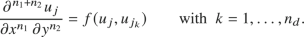
The displacements and the dilatations of the fictitious points are determined by means of the Taylor-based extrapolation method [35]. Consider the displacement ${\textbf{u}}_f = {\textbf{u}} ({\textbf{x}}_f)$ of a fictitious point, where ${\textbf{x}}_f = \{ x_f, y_f, z_f \}^{\top }$. We name ${\textbf{u}}_b = {\textbf{u}} ({\textbf{x}}_b)$ the displacement of the boundary point with the minimum distance from that fictitious point (nearest-point strategy). The Taylor series expansion of ${\textbf{u}}_f$ about ${\textbf{x}}_b = \{ x_b, y_b, z_b \}^{\top }$ truncated at the maximum order $n_{max} \ge 1$ is given by

(33)

where n is the global order ($n=1$ is related to the gradient, $n=2$ to the Hessian matrix, etc.) and $n_1$, $n_2$ and $n_3$ are the orders respectively in x, y and z directions.

Similarly, consider the dilatation $\theta _f = \theta ({\textbf{x}}_f)$ of a fictitious point and the dilatation $\theta _b = \theta ({\textbf{x}}_b)$ of the boundary point closest to ${\textbf{x}}_f$. The Taylor series expansion of $\theta _f$ about ${\textbf{x}}_b$ truncated at the maximum order $n_{max}-1$ is given by

(34)

with $n_3 = n-n_1-n_2$. Note that the dilatation is a measure of the strain, thus its truncation of the Taylor expansion occurs with 1 order less than that of the displacement.

This method allows to determine the displacement field and the dilatation field in the fictitious layer $\mathcal {F}$ as a function of the respective fields in the body $\mathcal {B}$. Since the displacement and dilatation fields in $\mathcal {F}$ are approximated by means of a Taylor series expansion, more accurate results are obtained by increasing the truncation order $n_{\max }$ or by reducing the thickness of the fictitious layer.

The new bonds between real and fictitious points, called “fictitious bonds”, are the interactions that are lacking in the peridynamic models without fictitious layer. The Taylor-based extrapolation method provides the displacement and dilatation values of the fictitious points, which are required to compute the pairwise forces of the fictitious bonds. In this way, the proposed method is able to mitigate the surface effect.

3.2 Peridynamic boundary conditions

We propose hereinafter a novel method to impose the boundary conditions in a peridynamic way when using the previously described fictitious layer method [35]. The desired boundary conditions are applied solely on the boundary points, exactly as in classical continuum mechanics. However, the influence of the boundary conditions on the body is non-local thanks to the Taylor-based extrapolation method. This concept is explained for Dirichlet and Neumann boundary conditions in the following.

A constraint $\overline{{\textbf{u}}}$ imposed in a boundary point ${\textbf{x}}_b$ is simply given as

$$\begin{aligned} {\textbf{u}} ({\textbf{x}}_b) = \overline{{\textbf{u}}} \, . \end{aligned}$$

(35)

This boundary condition determines the displacement field in the fictitious layer through the Taylor-based extrapolation method (by substituting Eq. 35 in Eq. 33). Therefore, the influence of the constraint can be seen as distributed in the whole thickness of the fictitious layer, as suggested in [21, pp. 29–30].

An external load per unit area $\overline{{\textbf{p}}}$ applied to a boundary point ${\textbf{x}}_b$ is expressed by means of the peridynamic concept of force flux (see Eq. 30):

$$\begin{aligned} \varvec{\tau } ({\textbf{x}}_b,{\textbf{n}}) = \overline{{\textbf{p}}} \, , \end{aligned}$$

(36)

where ${\textbf{n}}$ is the unit vector perpendicular to the boundary in ${\textbf{x}}_b$. By definition of force flux, $\varvec{\tau } ({\textbf{x}}_b,{\textbf{n}})$ is the sum of the pairwise forces (per unit area) of all the bonds passing through ${\textbf{x}}_b$. Since point ${\textbf{x}}_b$ lies on the boundary, all the bonds involved in Eq. 36 are fictitious bonds. On the one hand, the pairwise forces of those bonds applied to the fictitious points, which do not constitute new degrees of freedom, are ignored. On the other hand, the corresponding pairwise forces applied to the real points are the only ones “perceived” by the body. For how the magnitude of those forces is computed (see Eq. 20), the boundary condition in point ${\textbf{x}}_b$ affects the displacement in a sphere of radius $2\delta$ centered in ${\textbf{x}}_b$. Therefore, the external load, expressed by means of the definition of the force flux, is distributed on the points in a layer of thickness $2\delta$ within the body, as suggested in [21, pp. 30–32].

Fig. 10

Uniform peridynamic grid of real nodes (solid dots) and fictitious nodes (empty dots)

The proposed method for imposing the boundary conditions, which makes use of the Taylor-based extrapolation on the fictitious layer, defines a peridynamic way to distribute the constrains or the loads in the non-local region near the boundary.

Remark 1

The reaction force acting on a boundary point ${\textbf{x}}_b$, due to a constraint imposed as in Eq. 35, can be computed as the force flux in ${\textbf{x}}_b$ in the direction of the unit vector ${\textbf{n}}$ perpendicular to the boundary, i.e., $\varvec{\tau } ({\textbf{x}}_b, {\textbf{n}})$.

Remark 2

The zero-traction boundary condition is sometimes applied by removing the fictitious layer in literature [22]. However, in order to maintain the correction of the surface effect, we suggest to keep the fictitious layer and impose the condition $\varvec{\tau } ({\textbf{x}}_b,{\textbf{n}}) = 0$ to all the points of that boundary.

4 Numerical implementation

In order to discretize the domain, a mesh-free method is adopted [36, 41]. For simplicity sake, the peridynamic grid consists of a finite number of equally-spaced nodes, as shown in Fig. 10. Each peridynamic node is representative of a finite volume $\varDelta V = h \varDelta x^2$, where $\varDelta x = \varDelta y$ is the grid spacing and h is the thickness of the body. Please note that the most external real nodes do not lie exactly on the boundary of the body since the nodes are positioned at the center of the volume $\varDelta V$. The ratio between the horizon and the grid spacing is defined as $\overline{m}$-ratio: $\overline{m} = \delta /\varDelta x$. The value of this parameter determines the density of peridynamic nodes within a neighborhood. Furthermore, the fictitious layer (empty dots in Fig. 10) is added to the real body to complete the neighborhoods of the nodes near the boundary.

4.1 Numerical Taylor-based extrapolation method

The Taylor-based extrapolation procedure in the discretized model aims to determine the values of the variables of the fictitious nodes (displacements u and v respectively in x and y directions and dilatations $\theta$ in the case of a peridynamic 2-dimensional body). The numerical procedure to determine, for instance, the displacement $u_i$ in a fictitious node i with coordinates $(x_i, y_i)$ is carried out as follows:

• find the real node of index j closest to node i;

• perform a Taylor series expansion of $u_i$ about node j with coordinates $(x_j, y_j)$:

  

  (37)

  where $u_j$ and are the displacement of node j and its derivatives, $n_{max}$ is the maximum order of the truncated Taylor series, $n_1$ and $n_2$ are the orders respectively in x and y directions and n is the global order so that $n_2 = n-n_1$.

Since the coordinates of nodes i and j are known, the displacement $u_i$ in Eq. 37 is written as a function of the displacement $u_j$ and its derivatives. However, we aim to express $u_i$ as a function solely of the displacement of the real nodes. The total number of derivatives of $u_j$, considered before truncating the Taylor series, is $n_d = (n_{max} (n_{max}+1) /2)-1$. They can be determined as functions of the displacements of the $n_d$ real nodes near node j by following another Taylor-based extrapolation procedure:

• find the $n_d$ real nodes with indices $j_k$ closest to node j, where $k=1,\dots ,n_d$ (see Remark below for the conditions on the node search);

• for each of those nodes with coordinates $(x_{j_k}, y_{j_k})$, perform a Taylor series expansion of their displacements $u_{j_k}$ about node j:

  

  (38)

• solve the system of equations in Eq. 38 to obtain the derivatives of $u_j$ as a function of the displacements $u_j$ and $u_{j_k}$:

  

  (39)

Therefore, by combining Eqs. 37 and 39 , the displacement of a fictitious node is a function only of the displacements of some real nodes. Note that the adopted nearest-node startegy is really simple to implement also for complex geometries. This procedure can be applied to determine the displacements u and v and the dilatations $\theta$ of all the fictitious nodes. In the case of the dilatations, the truncation order $n_{max}$ must be replaced by $n_{max}-1$.

Remark 3

There might be some cases in which the system of equations (Eq. 38) is not solvable for the nodes $j_k$ that are the closest to node j. For instance, if we want to determine the second derivative in x direction, the nodes $j_k$ must include at least two $x_{j_k}$ coordinates different from each other and from $x_j$ (see example in Sect. 4.5). However, given the adoption a uniform grid in which nodes on the same lines share the same coordinates, this condition is not always met when searching for nodes $j_k$ via the closest-node strategy without any additional condition. Therefore, in order for the system of equations to be solvable, the nodes $j_k$ should comprise at least $n_1$ different $x_{j_k}$ coordinates and $n_2$ different $y_{j_k}$ coordinates (excluding $x_j$ and $y_j$) for each derivative of order $n_1$ in x direction and $n_2$ in y direction.

In the following we present an example for determining the displacement $u_i$ of a fictitious node i near a corner of the body by means of the Taylor-based extrapolation method with $n_{max}=2$. As shown in Fig. 11, the node j near the corner is the real node closest to node i. Thus, the displacement $u_i$ can be given via a Taylor series expansion about node j (see Eq. 37) as

(40)

where $l_x = x_i-x_j$ and $l_y = y_i-y_j$. Note that the number of derivatives of the displacement $u_j$ is $n_d=5$.

Fig. 11

Taylor-based extrapolation method for a fictitious node i near a corner of the body: node j is the real node closest to node i and nodes $j_k$ with $k = 1,\dots ,5$ are the real nodes closest to node j

As shown in Fig. 11, $j_k$ with $k = 1,\dots ,5$ are the 5 indices of the real nodes closest to node j. Note that, in order to be compliant with the condition given in Remark 3, the search for the closest nodes should be carried out in terms of Manhattan distance. A system of 5 equations is written by performing a Taylor series expansion of $u_{j_k}$ about node j (see Eq. 39):

(41)

The factors of the Taylor series expansions, which are multiplied by the derivatives of $u_j$, are easily derived from Fig. 11. After some manipulations, the system in Eq. 41 yields:

(42)

Therefore, by substituting Eq. 42 in Eq. 40, the displacement $u_i$ of the fictitious node is expressed as a function solely of the displacements of the real nodes. This procedure can be repeated for the required variables of all the fictitious nodes.

4.2 Numerical formulation of peridynamics

Consider a real node i, as shown in Fig. 12. The neighborhood $\mathcal {H}_i$ of node i embeds the complete volume of the nearest nodes and the partial volume of the nodes near the horizon limit. Therefore, all the nodes with at least a portion of their own volume within the horizon limit are considered part of the neighborhood $\mathcal {H}_i$. For each family node j, the volume correction coefficient $\beta _{ij} \le 1$ is computed as the fraction of volume actually contained in the neighborhood [36]. If $\varDelta V$ of node j is completely inside the neighborhood, then $\beta _{ij}=1$.

Fig. 12

The neighborhood $\mathcal {H}_i$ of a node i is constituted by the nodes (black dots) with at least a part of their volume inside the horizon (gray line). The volume correction coefficient $\beta$ is the fraction of the volume of the family nodes j within the horizon limit

The bond ij, which connects node i to node j, could be either a real bond or a fictitious bond. In both cases, its reference scalar state $\underline{x}_{ij}$, Gaussian influence function $\underline{\omega }_{ij}$ and inclination $\phi _{ij}$ with respect to the x-axis, can be computed from the coordinates of the two nodes. Under the assumption of small displacements, the extension scalar state of bond ij is given as

$$\begin{aligned} \underline{e}_{ij} = (u_j - u_i) \cos \phi _{ij} + (v_j - v_i) \sin \phi _{ij} \, , \end{aligned}$$

(43)

where $u_i$ and $u_j$ are the displacements in x direction respectively of nodes i and j and $v_i$ and $v_j$ are the displacements in y direction respectively of nodes i and j. If the family node j is fictitious, Eq. 43 holds and $u_j$ and $v_j$ are determined as a function of the displacements of the real nodes by the Taylor-based extrapolation method exposed in Sect. 4.1.

The weighted volume of node i is evaluated by performing a mid-point Gauss quadrature from Eq. 13:

$$\begin{aligned} m_i = \sum _{j \in \mathcal {H}_i} \underline{\omega }_{ij} \, \underline{x}_{ij}^2 \, \beta _{ij} \, \varDelta V \, . \end{aligned}$$

(44)

Since the neighborhoods of all the real nodes are complete thanks to the presence of the fictitious nodes, the weighted volume is constant in the whole body. Furthermore, the value of the weighted volume of the real nodes is assigned also to the fictitious nodes, as dictated by the Taylor-based extrapolation method.

Similarly, the dilatation of a real node i is computed from Eq. 14 as

$$\begin{aligned} \theta _i = \frac{c_{\theta }}{m_i} \sum _{j \in \mathcal {H}_i} \underline{\omega }_{ij} \, \underline{x}_{ij} \, \underline{e}_{ij} \, \beta _{ij} \, \varDelta V \, . \end{aligned}$$

(45)

On the other hand, the dilatations of the fictitious nodes are determined as a function of the dilatations of the real nodes by means of another Taylor-based extrapolation, as illustrated in Sect. 4.1.

The magnitude of the pairwise force density in bond ij is given from Eq. 20 as

$$\begin{aligned} \textrm{f}_{ij} {=} \left[ k_{\theta } \left( \frac{\theta _i}{m_i} {+} \frac{\theta _j}{m_j} \right) \underline{\omega }_{ij} \, \underline{x}_{ij} {+} k_e \left( \frac{1}{m_i} {+} \frac{1}{m_j} \right) \underline{\omega }_{ij} \, \underline{e}_{ij} \right] \beta _{ij} \, . \nonumber \\ \end{aligned}$$

(46)

Note that the constants $k_{\theta }$ and $k_e$ are determined by the constitutive modelling of the peridynamic theory, the parameters $m_i$, $m_j$, $\underline{\omega }_{ij}$, $\underline{x}_{ij}$ and $\beta _{ij}$ depend only on the geometric coordinates of the nodes in the reference configuration and the variables $\underline{e}_{ij}$, $\theta _i$ and $\theta _j$ can be written as functions of the displacements of the real nodes (by using the proposed Taylor-based extrapolation method for the variables of the fictitious nodes). Therefore, by combining Eqs. 43–46 together, one can write an equation for each bond ij, either real or fictitious, to relate the magnitude $\textrm{f}_{ij}$ of its pairwise force density to the displacements of the real nodes.

Finally, under the assumption of small deformation, the peridynamic equilibrium equation (multiplied by the node volume $\varDelta V$) is written for every real node i as

$$\begin{aligned} - \sum _{j \in \mathcal {H}_i} \textrm{f}_{ij} \, {\textbf{m}}_{ij} \, \varDelta V^2 = {\textbf{b}}_i \, \varDelta V \qquad \forall i \in \mathcal {B} \end{aligned}$$

(47)

where ${\textbf{m}}_{ij} = \{ \cos \phi _{ij}, \, \sin \phi _{ij} \}^{\top }$ is the bond direction in the reference configuration and ${\textbf{b}}_i$ is the external force density vector applied to node i. The system of equations in Eq. 47 can be rewritten in the standard form

$$\begin{aligned} {\textbf{K}} \, \widetilde{{\textbf{u}}} = \widetilde{{\textbf{f}}} \, , \end{aligned}$$

(48)

where ${\textbf{K}}$ is the peridynamic stiffness matrix (size: $2N \times 2N$), $\widetilde{{\textbf{u}}}$ is the displacement vector (size: $2N \times 1$) and $\widetilde{{\textbf{f}}}$ is the force vector (size: $2N \times 1$). N is the number of real nodes. The stiffness matrix ${\textbf{K}}$ includes the contributions of the fictitious bonds, thus it embeds the correction of the surface effect by means of the Taylor-based extrapolation method.

4.3 Numerical evaluation of the peridynamic stress tensor

This section deals with the numerical procedure to compute the peridynamic stress tensor. The theoretical background can be found in Sect. 2.2.

In the discretized peridynamic model, we name the nodes corresponding to the points ${\textbf{x}}$, ${\textbf{x}}'$ and ${\textbf{x}}''$ (see Fig. 2) respectively as i, j and k. Under the assumption of point i being in the bulk of a body subjected to a homogeneous deformation (see Eq. 23), the peridynamic stress tensor can be computed as

$$\begin{aligned} \varvec{\tau }_{i} = \frac{1}{2} \sum _{k \in \mathcal {H}_i} r_{ik} \, \textrm{f}_{ik} \, {\textbf{m}}_{ik} \otimes {\textbf{m}}_{ik} \, \varDelta V \, , \end{aligned}$$

(49)

where $r_{ik}$ is the length of the bond ik. Equation 49 provides a good approximation also in the case of non-homogeneous deformations if the horizon $\delta$ is sufficiently small, as shown in [10] for bond-based peridynamics. However, Eq. 49 is not valid for nodes near the boundary which are affected by the surface effect (if no fictitious layer is employed).

In order to compute numerically the peridynamic stress tensor $\varvec{\tau }_{i}$ in a general node i, also not in the bulk of the body, the integrand of Eq. 22 should be evaluated for each bond jk between node j and node k. The differential volume $\mathop {}\! \textrm{d} {V}_{{\textbf{x}}''}$ corresponds simply to the finite volume of node k, i.e., $\varDelta V$. On the other hand, we must distinguish two types of bonds, which are shown in Fig. 13, to determine $\varDelta s$ as the corresponding of the differential length $\mathop {}\! \textrm{d} {s}$ of point ${\textbf{x}}'$ in the direction of the bond ${\textbf{m}}$:

$$\begin{aligned} \varDelta s = {\left\{ \begin{array}{ll} \frac{\varDelta x}{| \cos \phi _{jk} |} &{} \text {if}{ \ } | \cos \phi _{jk} | \ge \frac{\sqrt{2}}{2} \, , \\ \frac{\varDelta y}{ | \sin \phi _{jk} |} &{} \text {if}{ \ } | \cos \phi _{jk} | < \frac{\sqrt{2}}{2} \, , \\ \end{array}\right. } \end{aligned}$$

(50)

where the trigonometric functions are within the absolute value because $\varDelta s > 0$. In the former case bond jk is a type-A bond and, in the latter, a type-B bond, which are respectively shown in Fig. 13a and b. A type-A bond contributes to $\varvec{\tau }_{i}$ if it intersects the area $\varDelta A_i^{\textrm{A}} = h \varDelta y$ passing through node i perpendicular to x direction, where h is the thickness of the 2-dimensional body. Similarly, a type-B bond contributes to $\varvec{\tau }_{i}$ if it intersects the area $\varDelta A_i^{\textrm{B}} = h \varDelta x$ passing through node i perpendicular to y direction. Therefore, the peridynamic stress tensor in a node i is given as

$$\begin{aligned} \begin{aligned} \varvec{\tau }_{i} =&\frac{1}{2} \sum _{\varvec{\xi }_{jk} \, \cap \, \varDelta A_i^{\textrm{A}} \, \ne \emptyset } \alpha _{jk} \, \textrm{f}_{jk} \, {\textbf{m}}_{jk} \otimes {\textbf{m}}_{jk} \, \frac{\varDelta x}{| \cos \phi _{jk} |} \varDelta V \\&+ \frac{1}{2} \sum _{\varvec{\xi }_{jk} \, \cap \, \varDelta A_i^{\textrm{B}} \, \ne \emptyset } \alpha _{jk} \, \textrm{f}_{jk} \, {\textbf{m}}_{jk} \otimes {\textbf{m}}_{jk} \, \frac{\varDelta y}{| \sin \phi _{jk} |} \varDelta V \, , \end{aligned} \end{aligned}$$

(51)

where $\textrm{f}_{jk}$ is the magnitude of the pairwise force density of bond jk obtained with Eq. 46, ${\textbf{m}}_{jk} = \{ \cos \phi _{jk}, \, \sin \phi _{jk} \}^{\top }$ is the bond direction and $\alpha _{jk}$ is a correction coefficient, given as:

$$\begin{aligned} \alpha _{jk} = {\left\{ \begin{array}{ll} \frac{1}{2} &{} \text {if}{ \ } j=i { \ \text {or} \ } k=i \, , \\ \frac{1}{2} &{} \text {if}{ \ } \varvec{\xi }_{jk} \cap \partial A_i \ne \emptyset \, , \\ 1 &{} \text {if}{ \ } \varvec{\xi }_{jk} \cap \left( \varDelta A_i \setminus \partial A_i \right) \ne \emptyset \, , \\ \end{array}\right. } \end{aligned}$$

(52)

where $\partial A_i$ is the boundary of the area $\varDelta A_i$, which can be referred either to type-A bonds ($\varDelta A_i^{\textrm{A}}$) or to type-B bonds ($\varDelta A_i^{\textrm{B}}$). The different cases in Eq. 52 are illustrated in Fig. 14:

• in the case with $j=i$ (see Fig. 14a), since only half of the length $\varDelta s$ related to node j is on the opposite side of $\varDelta A_i$ with respect to node k, then $\alpha _{jk}=1/2$;

• similarly, in the case with $k=i$ (see Fig. 14b), since only half of the volume $\varDelta V$ of node k is on the opposite side of $\varDelta A_i$ with respect to node j, then $\alpha _{jk}=1/2$;

• in the case that the bond intersects the boundary of $\varDelta A_i$, i.e., $\varvec{\xi }_{jk} \cap \partial A_i \ne \emptyset$, since $\partial A_i$ overlaps the boundary of the area of another node (node q in Fig. 14c), the magnitude of the pairwise force density of bond jk is equally shared between those nodes and, therefore, $\alpha _{jk}=1/2$;

• in the case that the bond intersects $\varDelta A_i$ not on its boundary, i.e., $\varvec{\xi }_{jk} \cap \left( \varDelta A_i \setminus \partial A_i \right) \ne \emptyset$ (see Fig. 14d), the magnitude of the pairwise force density of bond jk contributes entirely to $\varvec{\tau }_{i}$ and, therefore, $\alpha _{jk}=1$;

Moreover, to improve the computational efficiency, one might remove the factors 1/2 in Eq. 51 and consider each bond just once (for example consider only bond jk and not bond kj).

Fig. 13

Examples of type-$\textrm{A}$ and type-$\textrm{B}$ bonds for the computation of the peridynamic stress tensor $\varvec{\tau }_i$ in node i. The bonds contribute to $\varvec{\tau }_i$ only if they intersect the corresponding area $\varDelta A_i$

Fig. 14

Values of the correction coefficient $\alpha _{jk}$ for different types of intersection between bond jk and area $\varDelta A_i$. These examples consider only type-A bonds, but the same concepts are valid also for type-B bonds

The proposed numerical procedure to compute the peridynamic stress tensor is used to highlight the surface effect in a 2-dimensional body in Sect. 2.4. Figures 7 and 8 show that the numerical computation of the peridynamic stress tensor is very close to the analytical solutions, obtained in Sect. 2.2, for nodes with a complete neighborhood.

4.4 Numerical evaluation of the force flux

Consider a finite area $\varDelta A$ which constitutes one of the sides of the volume cell of a node, as shown in Fig. 15. The numerical procedure to compute the peridynamic force flux through the finite area $\varDelta A$ is exposed in this section.

Fig. 15

Values of the correction coefficient $\alpha _{jk}$ for different types of intersection between bond jk and area $\varDelta A$

The force flux $\varvec{\tau } ({\textbf{x}}, {\textbf{n}})$ of a point ${\textbf{x}}$ in a direction ${\textbf{n}}$ is interpreted in Sect. 2.3 as the sum of the pairwise forces per unit area of all the bonds intersecting the differential area $\mathop {}\! \textrm{d} {A}_{{\textbf{x}}}$ on the plane $\mathcal {P}$ in ${\textbf{x}}$, where $\mathcal {P}$ is the plane passing through ${\textbf{x}}$ perpendicular to ${\textbf{n}}$ (see Figs. 4 and 5 ). Therefore, the force flux through $\varDelta A$ can be discretized from Eqs. 30 and 32 as

$$\begin{aligned} \varvec{\tau } ({\textbf{x}}, {\textbf{n}}) = \frac{1}{\varDelta A} \sum _{\begin{array}{c} \varvec{\xi }_{jk} \, \cap \, \varDelta A \, \ne \emptyset \\ {\textbf{m}}_{jk} \cdot {\textbf{n}} > 0 \end{array}} \alpha _{jk} \, \textrm{f}_{jk} \, {\textbf{m}}_{jk} \, \varDelta V^2 \, , \end{aligned}$$

(53)

where ${\textbf{x}}$ and ${\textbf{n}}$ are respectively the centroid and the normal of $\varDelta A$, $\textrm{f}_{jk} \, {\textbf{m}}_{jk} \, \varDelta V^2$ is the pairwise force of any bond jk intersecting $\varDelta A$ and $\alpha _{jk}$ is the correction coefficient given by Eq. 52 (see also in Fig. 15a, b the possible cases in the computation of the force flux). Note that, in order to improve the computational efficiency, the factor 1/2 is removed because only bonds satisfying the condition ${\textbf{m}}_{jk} \cdot {\textbf{n}} > 0$ are considered. Since we are mostly interested in the force flux computed at the boundary of the body to impose Neumann boundary conditions, this concept is further analyzed in the next section.

4.5 Numerical implementation of the peridynamic boundary conditions

The real nodes closest to the boundary are not exactly on the boundary of the body (see Fig. 10). Therefore, by following the concepts exposed in Sect. 3.2, the boundary conditions in the discretized model should be imposed on the sides of the volume cells which overlap the boundary. We introduce a new cathegory of nodes, called “boundary nodes”, at which the boundary conditions are imposed. Each boundary node is positioned at the centroid of the side of the volume cell of the nodes closest to the boundary and is representative of the finite area $\varDelta A_b$ of that side, as shown in Fig. 16. As the fictitious nodes, the boundary nodes do not constitute new degrees of freedom because their displacements are determined as a function of the displacements of the real nodes by means of the Taylor-based extrapolation method.

Fig. 16

Boundary nodes at the boundary of the body: each node b is representative of a finite area $\varDelta A_b$ and is associated to the normal ${\textbf{n}}_b$ external to the body

Suppose that the problem requires a constraint $\overline{u}$ for the displacement $u_b$ in x direction of a boundary node b, condition given as $u_b = \overline{u}$. The Taylor-based extrapolation method is applied to the boundary node exactly as done for the fictitious nodes in Sect. 4.1. The following procedure is valid also for $\overline{u}=0$. The displacement $u_b$ of the boundary node b with coordinates $(x_b, y_b)$ is determined by a Taylor series expansion about node j with coordinates $(x_j, y_j)$ as

(54)

where node j is the real node closest to node b. The $n_d$ derivatives of $u_j$ can be expressed as functions of the displacements of the $n_d$ real nodes close to node j. Therefore, the Dirichlet boundary condition can be written as a function of the displacements of some real nodes:

$$\begin{aligned} \overline{u} = f (u_j, u_{j_k}) \qquad \text {with}{ \ } k = 1,\dots ,n_d . \end{aligned}$$

(55)

For example, we consider the case shown in Fig. 17 with a truncation order $n_{max}=2$. The Taylor series expansion of the displacement $u_b$ about node j is given as

(56)

In order to determine the two derivatives in x direction of Eq. 56, we find nodes $j_1$ and $j_2$, shown in Fig. 17, as the nodes closest to node j having x coordinates different from each other and from $x_j$ (see Remark 3). We write the system of equations given by the Taylor series expansions of $u_{j_1}$ and $u_{j_2}$ about node j, as in Eq. 38, and solve it to obtain the needed derivatives:

(57)

By substituting Eq. 57 in Eq. 56, the constraint condition $u_b = \overline{u}$ is given as a function of the displacements of some real nodes:

$$\begin{aligned} \overline{u} = \frac{15}{8} u_j - \frac{5}{4} u_{j_1} + \frac{3}{8} u_{j_2} \, . \end{aligned}$$

(58)

More in general, the proposed method allows to write the Dirichlet boundary conditions as functions of the displacement vector $\widetilde{{\textbf{u}}}$:

$$\begin{aligned} \overline{u} = f( \widetilde{{\textbf{u}}} ) \, . \end{aligned}$$

(59)

Fig. 17

Example of the Taylor-based extrapolation method used on a boundary node b

Suppose now that an external force per unit area $\overline{{\textbf{p}}}$ is applied to a boundary node b, as shown in Fig. 18. The Neumann boundary condition is written in terms of force flux through the area $\varDelta A_b$ associated to node b:

$$\begin{aligned} \varvec{\tau } ({\textbf{x}}_b, {\textbf{n}}_b) = \frac{1}{\varDelta A_b} \sum _{\begin{array}{c} \varvec{\xi }_{jk} \, \cap \, \varDelta A_b \, \ne \emptyset \\ {\textbf{m}}_{jk} \cdot {\textbf{n}}_b > 0 \end{array}} \alpha _{jk} \, \textrm{f}_{jk} \, {\textbf{m}}_{jk} \, \varDelta V^2 = \overline{{\textbf{p}}} \, , \end{aligned}$$

(60)

where ${\textbf{x}}_b$ is the position of node b and ${\textbf{n}}_b$ is the unit vector perpendicular to $\varDelta A_b$ external to the body. Since the pairwise force density of any bond can be expressed as a function of the displacements of the real nodes (see Sect. 4.2), also $\varvec{\tau } ({\textbf{x}}_b, {\textbf{n}})$ is a function of those displacements. Thus, Neumann boundary conditions can be written as functions of the displacement vector $\widetilde{{\textbf{u}}}$:

$$\begin{aligned} \overline{{\textbf{p}}} = f( \widetilde{{\textbf{u}}} ) \, . \end{aligned}$$

(61)

Fig. 18

Example of an external load $\overline{{\textbf{p}}}$ applied to a boundary node b

Since both Dirichlet and Neumann boundary conditions are given by equations in which the only unknowns are the displacements of the real nodes (see Eqs. 59 and 61 ), we gather all the boundary conditions in a matrix form as

$$\begin{aligned} {\textbf{B}} \, \widetilde{{\textbf{u}}} = \overline{{\textbf{c}}} \, , \end{aligned}$$

(62)

where ${\textbf{B}}$ is the matrix of the boundary conditions (size: $2N_b \times 2N$), $\widetilde{{\textbf{u}}}$ is the displacement vector (size: $2N \times 1$) and $\overline{{\textbf{c}}}$ is the vector of the known terms (size: $2N_b \times 1$). $N_b$ is the number of boundary nodes.

In order to include the boundary conditions (${\textbf{B}} \, \widetilde{{\textbf{u}}} = \overline{{\textbf{c}}}$) in the system of equations derived from the equilibrium of the real nodes (${\textbf{K}} \, \widetilde{{\textbf{u}}} = \widetilde{{\textbf{f}}}$), we conveniently use the technique of the Lagrange multipliers [5]. The vector of the Lagrange multipliers $\varvec{\lambda }$ (size: $2N_b \times 1$) is introduced in the system as

$$\begin{aligned} \begin{bmatrix} {\textbf{K}} &{} {\textbf{B}}^\top \\ {\textbf{B}} &{} {\textbf{0}} \\ \end{bmatrix} \begin{Bmatrix} \widetilde{{\textbf{u}}} \\ \varvec{\lambda } \\ \end{Bmatrix} = \begin{Bmatrix} \widetilde{{\textbf{f}}} \\ \overline{{\textbf{c}}} \\ \end{Bmatrix} \, . \end{aligned}$$

(63)

The displacement vector $\widetilde{{\textbf{u}}}$, extracted from the vector $\{ \widetilde{{\textbf{u}}}, \varvec{\lambda } \} ^\top$, is the solution to the system of equilibrium equations which satisfies the imposed boundary conditions.

5 Numerical examples

Several examples are presented to verify the reliability and accuracy of the proposed method. Whenever possible, the numerical peridynamic results are compared with the reference solutions derived from classical continuum mechanics. The reference solution coincides with the peridynamic solution only in the limit of the horizon $\delta$ approaching 0 [26, 43]. Therefore, the “difference” between these solutions includes two components: a discrepancy due to the different (local and non-local) formulations of the theories and the actual error given by the discretization and the implementation of the peridynamic model (either with or without the proposed method). The difference (in percentage) of the displacements between the peridynamic numerical results and the reference solution is computed at each node i as

$$\begin{aligned} \varvec{\epsilon }_i = \begin{Bmatrix} \epsilon _u \\ \epsilon _v \\ \end{Bmatrix}_i = \begin{Bmatrix} \displaystyle \frac{|u_i-u_{ref} ({\textbf{x}}_i)|}{\max (|\widetilde{{\textbf{u}}}_{ref}|)} \cdot 100 \\ \displaystyle \frac{|v_i-v_{ref} ({\textbf{x}}_i)|}{\max (|\widetilde{{\textbf{u}}}_{ref}|)} \cdot 100 \\ \end{Bmatrix} \, , \end{aligned}$$

(64)

where $u_i$ and $v_i$ are the displacements of node i, $u_{ref} ({\textbf{x}}_i)$ and $v_{ref} ({\textbf{x}}_i)$ are the displacements obtained with the reference solution at the position ${\textbf{x}}_i$ of node i and $\widetilde{{\textbf{u}}}_{ref}$ is the displacement vector obtained with the reference solution at all the nodes. The reference solution is defined for each example by providing either the analytical solution (if possible), or the results obtained with the Finite Element Method.

For simplicity sake, we consider a plate under plane stress conditions with different boundary conditions. The parameters adopted for the simulations of the plate are reported in Table 1. Firstly, we solve each example without adding the fictitious nodes. In this case, the boundary conditions are implemented by assigning the desired value of the constraints or loads to the most external nodes of the plate. In particular, Dirichlet boundary conditions are imposed by assigning to the nodes closest to the boundary the value of the displacement computed with the reference solution. Then, the same examples are solved by adopting the proposed Taylor-based extrapolation method and by implementing the boundary conditions as described in Sect. 4.5.

Table 1 Parameters of the plate and of its discretization

5.1 Plate under traction

The boundary conditions of the first example are shown in Fig. 19. The analytical solution is given by classical continuum mechanics as

$$\begin{aligned} {\textbf{u}} ({\textbf{x}}) = \begin{Bmatrix} u (x,y) \\ v (x,y) \\ \end{Bmatrix} = \begin{Bmatrix} \displaystyle \frac{\overline{p}}{E} \left( x+\frac{\ell _x}{2} \right) \\ \displaystyle \frac{-\nu \, \overline{p}}{E} \left( y+\frac{\ell _y}{2} \right) \\ \end{Bmatrix} \, , \end{aligned}$$

(65)

where $\overline{p}$ is the traction load.

Fig. 19

Boundary conditions for the plate under the traction $\overline{p}={1}{\hbox {MPa}}$

The plots in Fig. 20 show the difference of the displacement field, computed without adopting any correction to the peridynamic model, with respect to the reference solution. The surface effect and the approximated way of imposing the boundary conditions lead to large errors near the boundary of the plate, especially near the corners. On the other hand, there are no fluctuations in the displacement field when the proposed Taylor-based extrapolation method with $n_{max}=1$ is employed. The differences of the displacement field of the corrected model (see Fig. 21) decrease sensibly with respect to those obtained without corrections at the boundary. Similar results are obtained by choosing higher orders for the Taylor-based extrapolation.

Fig. 20

Displacement field differences between the peridynamic numerical results for $\overline{m} = 3$ and the reference solution (obtained with the analytical solution in Eq. 65) in the plate under traction obtained without corrections at the boundary. Note that the colormaps refer to different values in the two plots

Fig. 21

Displacement field differences between the peridynamic numerical results for $\overline{m} = 3$ and the reference solution (obtained with the analytical solution in Eq. 65) in the plate under traction obtained by means of the Taylor-based extrapolation method with $n_{max}=1$. Note that the colormaps refer to different values in the two plots

In the case adopting the proposed method, the error can be further reduced by increasing the accuracy of the integration over the neighborhoods, i.e., by increasing $\overline{m}$ [36]. In order to show this, we compute the relative difference (in percentage) at a node i as

$$\begin{aligned} \varvec{\epsilon }_i^{rel} = \begin{Bmatrix} \epsilon _u^{rel} \\ \epsilon _v^{rel} \\ \end{Bmatrix}_i = \begin{Bmatrix} \displaystyle \frac{|u_i-u_{ref} ({\textbf{x}}_i)|}{|u_{ref} ({\textbf{x}}_i)|} \cdot 100 \\ \displaystyle \frac{|v_i-v_{ref} ({\textbf{x}}_i)|}{|v_{ref} ({\textbf{x}}_i)|} \cdot 100 \\ \end{Bmatrix} \, . \end{aligned}$$

(66)

In the case employing the Taylor-based extrapolation on the fictitious nodes, the relative difference of every node inside the body is the same. Therefore, we gather in Table 2 the relative errors for different values of $\overline{m}$. We can observe that the relative differences decrease significantly as the value of $\overline{m}$ increase.

Table 2 Relative differences between the peridynamic numerical results and the reference solution in the plate under traction when improving the numerical integration by increasing $\overline{m}$

5.2 Plate under shear load

We present another example considering a plate under a shear load $\overline{p}$. Figure 22 shows the boundary conditions of this case. Classical continuum mechanics yield the following analytical solution:

$$\begin{aligned} {\textbf{u}} ({\textbf{x}}) = \begin{Bmatrix} u (x,y) \\ v (x,y) \\ \end{Bmatrix} = \begin{Bmatrix} \displaystyle \frac{2 \, (1+\nu ) \, \overline{p}}{E} \left( y+\frac{\ell _y}{2} \right) \\ \displaystyle 0 \\ \end{Bmatrix} \, . \end{aligned}$$

(67)

Fig. 22

Boundary conditions for the plate under the shear load $\overline{p}={1} {\hbox {MPa}}$

The differences of the displacement field, computed without corrections at the boundary, with respect to the reference solution are shown in Fig. 23. We observe that the differences are lower with respect to the case of the plate under traction in Sect. 5.1. However, as highlighted in Eq. 67, one would expect the displacements v in y direction to be 0 in the whole body. This fact is not verified in the numerical simulation because of the surface effect (see plot of the component $\tau _{22}$ of the peridynamic stress tensor in Fig. 8). This problem is completely solved by implementing the proposed Taylor-based extrapolation method with $n_{max}=1$, as shown in Fig. 24. Also, the differences of the displacements u in x direction decreases with respect to those obtained without corrections at the boundary. Similar results are obtained by choosing higher orders for the Taylor-based extrapolation.

Fig. 23

Displacement field differences between the peridynamic numerical results for $\overline{m} = 3$ and the reference solution (obtained with the analytical solution in Eq. 67) in the plate under shear load obtained without corrections at the boundary. Note that the colormaps refer to different values in the two plots

Fig. 24

Displacement field differences between the peridynamic numerical results for $\overline{m} = 3$ and the reference solution (obtained with the analytical solution in Eq. 67) in the plate under shear load obtained by means of the Taylor-based extrapolation method with $n_{max}=1$. Note that the colormaps refer to different values in the two plots

As in the case of the plate under traction, we compute the relative differences $\epsilon _u^{rel}$ with Eq. 66 for different values of $\overline{m}$ when implementing the proposed method in the case of the plate under shear load. For each $\overline{m}$, the relative differences of the displacements u are constant in the whole body also in this case and they are reported in Table 3. The numerical results show a significant reduction of the differences when the numerical integration is improved.

Table 3 Relative differences between the peridynamic numerical results and the reference solution in the plate under shear load when improving the numerical integration by increasing $\overline{m}$

5.3 Plate under sinusoidal load

In the previous examples, the linear variation of the displacement field was properly captured by the Taylor-based extrapolation with the order $n_{max} = 1$ (or higher). We investigate now an example in which the order of the Taylor-based extrapolation does not match the order of variation of the displacement field. The boundary conditions of this example are shown in Fig. 25. The force density applied thoughout the plate is given as

$$\begin{aligned} b(x,y) = \overline{b} \sin \left( \frac{\pi x}{\ell _x} - \frac{\ell _x}{2} \right) \sin \left( \frac{\pi y}{\ell _y} - \frac{\ell _y}{2} \right) \, , \end{aligned}$$

(68)

where $\overline{b} = 10^6 \, {\text {N}/\text {m}^{3}}$.

Fig. 25

Boundary conditions for the plate under the sinusoidal load b(x, y), where the origin of the reference system is at the center of the plate. Given the symmetry of the boundary conditions, the displacements v in y direction on the x-axis are fixed to be 0

The reference solution, shown in Fig. 26, is obtained with the Finite Element Method by means of a uniform grid with a spacing $\varDelta x_{ {F E M}} = \varDelta x/2$. The peridynamic nodes share the coordinates with some of the FEM nodes, so that the peridynamic results can be compared with the reference solution. We expect that, by increasing $n_{max}$, the Taylor-based extrapolation would approximate better the displacements of the fictitious layer.

Fig. 26

Displacement fields of the plate under the sinusoidal load obtained with the finite element method. Note that the colormaps refer to different values in the two plots

Figures 27 and 28 show the differences between the numerical results and the reference solution for the numerical models either without employing any correction for the surface effect or by adopting the Taylor-based extrapolation method. The differences are evidently reduced when the peridynamic model includes the Taylor-based extrapolation method. The aforementioned differences include two contributions: one due to the different (local and non-local) formulations of the theories and the other which is the actual error associated to the approximated numerical solution of the peridynamic equations. The two components of the difference cannot be separated since the analytical peridynamic solution is not available. However, the fluctuations of the differences near the boundaries due to the surface effect are evident in Figs. 27a and 28 a, in which no corrections at the boundary are adopted. On the other hand, by exploiting the Taylor-based extrapolation method, the magnitude of the differences decrease considerably and, also, their distribution near the boundaries becomes smoother with the increasing of the truncation order $n_{max}$, as shown in Figs. 27b–d and 28b–d. This is arguably because the numerical results are getting closer to the analytical peridynamic solution by correcting the surface effect and imposing in a proper way the boundary conditions.

Fig. 27

Differences of the displacements in x direction between the peridynamic numerical results for $\overline{m} = 3$ and the reference solution (obtained with the finite element method results, as shown in Fig. 26) in the plate under the sinusoidal load obtained either without corrections at the boundary or by adopting the Taylor-based extrapolation method with different orders $n_{max}$. Note that the colormaps refer to different values in the four plots

Fig. 28

Differences of the displacements in y direction between the peridynamic numerical results for $\overline{m} = 3$ and the reference solution (obtained with the finite element method results, as shown in Fig. 26) in the plate under the sinusoidal load obtained either without corrections at the boundary or by adopting the Taylor-based extrapolation method with different orders $n_{max}$. Note that the colormaps refer to different values in the four plots

6 Crack propagation near the boundaries

A qualitative study is hereinafter conducted to investigate the behavior of crack growth near the boundaries of the body. We compare the results provided by the proposed method with the solution obtained with peridynamics when no corrections for the surface effect are adopted and the boundary conditions are imposed in a local way, i.e., constraints and load are applied only at the nodes closest to the boundary. The surface effect near the new boundaries generated by the crack growth is not corrected in the present paper, but it will be dealt with in future works.

In order to model fracture phenomena, we introduce the scalar $\mu$ which yields the status of the bond (unbroken or broken) [41]:

$$\begin{aligned} \mu = {\left\{ \begin{array}{ll} 1 &{} \text {if}{ \ } s<s_c, \\ 0 &{} \text {otherwise,} \\ \end{array}\right. } \end{aligned}$$

(69)

where s is the stretch of the bond and $s_c$ is the critical stretch for plane stress conditions. These quantities are respectively computed as [25]

$$\begin{aligned} s= & {} \frac{\Vert \varvec{\xi } + \varvec{\eta } \Vert - \Vert \varvec{\xi } \Vert }{\Vert \varvec{\xi } \Vert } \, , \end{aligned}$$

(70)

$$\begin{aligned} s_c= & {} \sqrt{\frac{4 G_0}{9 E \delta }} \, , \end{aligned}$$

(71)

where $G_0$ is the energy release rate. The scalar $\mu$ is history-dependent since a broken bond cannot be restored. The equilibrium equation is therefore modified as

$$\begin{aligned} - \int _{\mathcal {H}_{{\textbf{x}}}} \mu \, {\textbf{f}}({\textbf{x}},{\textbf{x}}') \mathop {}\! \textrm{d} {V}_{{\textbf{x}}'} = {\textbf{b}}_{{\textbf{x}}} \, , \end{aligned}$$

(72)

and the damage at each node can be evaluated as [41]

$$\begin{aligned} \varphi _{{\textbf{x}}} = 1- \frac{\int _{\mathcal {H}_{{\textbf{x}}}} \mu \mathop {}\! \textrm{d} {V}_{{\textbf{x}}'}}{\int _{\mathcal {H}_{{\textbf{x}}}} \mathop {}\! \textrm{d} {V}_{{\textbf{x}}'}} \, . \end{aligned}$$

(73)

For the quasi-static crack propagation, the sequentially linear analysis used in [24] is employed:

• find the equilibrium with the given loads (if possible);

• if there are bonds with $s \ge s_c$, remove the contributions to the stiffness matrix of the 4 most stretched bonds;

• repeat the first steps until the equilibrium is not possible or there are no bonds with $s \ge s_c$.

Note that, when the Taylor-based extrapolation method is used, also the fictitious bonds can be broken along with the other bonds. If one or more fictitious bonds fail near a boundary where a Neumann boundary condition is applied, then not only the stiffness matrix should be modified accordingly by removing the contributions of the broken bonds, but also the same external tension should be applied solely through the residual unbroken fictitious bonds.

Fig. 29

Boundary conditions for a plate with a pre-existing crack (red line) for the case with Dirichlet boundary conditions

6.1 Crack propagation due to Dirichlet boundary conditions

The geometry and the boundary conditions of a plate with a pre-existing crack are shown in Fig. 29. The properties of the plate under plane stress conditions are: thickness $h={0.005} {m}$, Young’s modulus $E={1} {\hbox {GPa}}$, Poisson’s ratio $\nu =0.2$ and energy release rate $G_0 = {196} {\hbox {J}/\hbox {m}^2}$. The constraint is given as $\overline{u}={0.001} {\hbox {m}}$. A grid spacing $\varDelta x = {0.0025}{\hbox {m}}$ is used and $\overline{m} = 3$ is chosen.

The results obtained by means of the peridynamic model with no corrections at the boundary and with the proposed method are compared in Fig. 30, in which the difference of the displacements in a node i is computed as

$$\begin{aligned} \varvec{\epsilon }_i^{pd} = \begin{Bmatrix} \epsilon _u^{pd} \\ \epsilon _v^{pd} \\ \end{Bmatrix}_i = \begin{Bmatrix} \displaystyle \frac{|u_i^{uncorr}-u_i^{corr}|}{\max (|{\textbf{u}}^{corr}|)} \cdot 100 \\ \displaystyle \frac{|v_i^{uncorr}-v_i^{corr}|}{\max (|{\textbf{v}}^{corr}|)} \cdot 100 \\ \end{Bmatrix} \, , \end{aligned}$$

(74)

where ${\textbf{u}}^{corr}$ and ${\textbf{v}}^{corr}$ are the displacement fields respectively in x and y directions. The superscript uncorr stands for “uncorrected” (peridynamic model with no corrections at the boundaries) and corr for “corrected” (peridynamic model with the Taylor-based extrapolation method with $n_{max}=1$). It can be noticed that there are non-negligible differences near the crack tip that may lead to different crack paths.

Fig. 30

Differences in the displacement fields (for $\overline{m} = 3$) of the pre-cracked plate computed with and without the Taylor-based extrapolation method for the case with Dirichlet boundary conditions. Note that the colormaps refer to different values in the two plots

As shown by the damage of the nodes in the final configuration of the model with no corrections (see Fig. 31), the crack branches and reaches the upper edge of the plate in two separated paths. On the other hand, when the Taylor-based extrapolation method is adopted, the crack propagates to the upper edge in a unique path and there is no branching phenomenon. Hence, the crack path may change near the boundaries if the surface effect is mitigated and the boundary conditions are imposed in a “peridynamic way”.

Fig. 31

Crack propagation in the pre-cracked plate for the case with Dirichlet boundary conditions when no correction at the boundaries are adopted

Fig. 32

Crack propagation in the pre-cracked plate for the case with Dirichlet boundary conditions when the Taylor-based extrapolation method is used

6.2 Crack propagation due to Neumann boundary conditions

The geometry and the boundary conditions of a plate with a pre-existing crack are shown in Fig. 33. The properties of the plate under plane stress conditions are: thickness $h={0.005} {\hbox {m}}$, Young’s modulus $E= {1}{\hbox {GPa}}$, Poisson’s ratio $\nu =0.2$ and energy release rate $G_0 = {196}{\hbox {J}/\hbox {m}^2}$. The plate is under a traction of $\overline{p}= {1}{\hbox {MPa}}$. A grid spacing $\varDelta x = {0.0025}{\hbox {m}}$ is used and $\overline{m} = 3$ is chosen.

Fig. 33

Boundary conditions for a plate with a pre-existing crack (red line) for the case with Neumann boundary conditions

Fig. 34

Differences in the displacement fields (for $\overline{m} = 3$) of the pre-cracked plate computed with and without the Taylor-based extrapolation method for the case with Neumann boundary conditions. Note that the colormaps refer to different values in the two plots

Fig. 35

Crack propagation in the pre-cracked plate for the case with Neumann boundary conditions when no correction at the boundaries are adopted

Fig. 36

Crack propagation in the pre-cracked plate for the case with Neumann boundary conditions when the Taylor-based extrapolation method is used

As in Sect. 6.1, the differences between the displacements obtained with and without the proposed method are computed as in Eq. 74. The differences near the tip of the pre-existing crack (see Fig. 34) are non-negligible and they may lead to different crack behaviors. The crack paths, shown in Figs. 35 and 36 respectively for the case without and with boundary corrections, are indeed different between each other. Therefore, the crack behavior may be modified by the mitigation of the surface effect and the proper imposition of the Neumann boundary conditions.

7 Conclusions

Two issues arising near the boundary of a body modelled with ordinary state-based peridynamics are addressed:

• the surface effect, i.e., the stiffness fluctuation near the boundary;

• the current lack of standard strategies to impose the boundary conditions.

The surface effect has been studied numerically by evaluating the peridynamic stress tensor with a novel discretization method (see Sect. 4.3) and the characteristic hardening/softening behavior towards the boundary has been highlighted (see Figs. 7 and 8 ). This issue has been addressed by introducing a fictitious layer that completes the partial neighborhoods of the nodes near the boundary. We proposed a new version of the Taylor-based extrapolation method adopting the nearest-node strategy: the displacements of the fictitious nodes are expressed as functions of the displacements of the closest real nodes by means of multiple Taylor series expansions. In this way, the surface effect is mitigated.

The fictitious layer is also exploited to impose the boundary conditions in a peridynamic way. The boundary of the body is discretized by the so-called “boundary nodes”. As the fictitious nodes, the boundary nodes do not constitute new degrees of freedom because their displacements are obtained with the Taylor-based extrapolation method. On the one hand, Dirichlet boundary conditions are implemented by constraining the boundary node and, accordingly, the fictitious layer mitigates the surface effect. On the other hand, Neumann boundary conditions are applied, via the numerical computation of the force flux at the boundary, to the bonds involving the fictitious nodes. Therefore, the boundary conditions are imposed in a “peridynamic way”.

Several numerical examples were presented to verify the accuracy of the proposed method. The numerical results obtained with the Taylor-based extrapolation method show a great improvement with respect to the peridynamic models without corrections at the boundary. Furthermore, the order of the Taylor-based extrapolation can be increased until the undesired fluctuations of the numerical results become negligible for the application of interest. It is also shown that the numerical integration of the peridynamic equilibrium equation plays a fundamental role, so that the numerical results are improved even further by increasing the value of the $\overline{m}$-ratio.

Moreover, we carried out a qualitative study on crack propagation near the boundaries by comparing the results obtained by means of the proposed method with those of the peridynamic model without boundary corrections. We presented two numerical examples in which the crack paths are different because of the difference in the displacement fields. This highlights the importance of mitigating the surface effect and of imposing properly the peridynamic boundary conditions.

References

Bobaru F, Foster J, Geubelle P, Silling S (2016) Handbook of peridynamic modeling. CRC Press, Boca Raton
Bobaru F, Ha Y (2011) Adaptive refinement and multiscale modeling in 2d peridynamics. J Multiscale Comput Eng 9(6), 635–659 (2011). https://digitalcommons.unl.edu/mechengfacpub/98
Bobaru F, Yang M, Alves L, Silling S, Askari E, Xu J (2009) Convergence, adaptive refinement, and scaling in 1d peridynamics. Int J Numer Meth Eng 77(6):852–877. https://doi.org/10.1002/nme.2439
Butt S, Meschke G (2021) Peridynamic analysis of dynamic fracture: influence of peridynamic horizon, dimensionality and specimen size. Comput Mech. https://doi.org/10.1007/s00466-021-02017-1
Carrera E, Pagani A, Petrolo M (2013) Use of Lagrange multipliers to combine 1d variable kinematic finite elements. Comput Struct 129:194–206. https://doi.org/10.1016/j.compstruc.2013.07.005
Chen J, Qingdao P, Jiao Y, Jiang W, Zhang Y (2020) Peridynamics boundary condition treatments via the pseudo-layer enrichment method and variable horizon approach. Math Mech Solids 1:1–36. https://doi.org/10.1177/1081286520961144
Chen Z, Bakenhus D, Bobaru F (2016) A constructive peridynamic kernel for elasticity. Comput Methods Appl Mech Eng 311:356–373. https://doi.org/10.1016/j.cma.2016.08.012
Chen Z, Bobaru F (2015) Selecting the kernel in a peridynamic formulation: a study for transient heat diffusion. Comput Phys Commun 197:51–60. https://doi.org/10.1016/j.cpc.2015.08.006
Diehl P, Prudhomme S, Lévesque M (2019) A review of benchmark experiments for the validation of peridynamics models. J Peridyn Nonlocal Model 1(1):14–35. https://doi.org/10.1007/s42102-018-0004-x
Fallah A, Giannakeas I, Mella R, Wenman M, Safa Y, Bahai H (2020) On the computational derivation of bond-based peridynamic stress tensor. J Peridyn Nonlocal Model 2(4):352–378. https://doi.org/10.1007/s42102-020-00036-9
Galvanetto U, Mudric T, Shojaei A, Zaccariotto M (2016) An effective way to couple fem meshes and peridynamics grids for the solution of static equilibrium problems. Mech Res Commun 76:41–47. https://doi.org/10.1016/j.mechrescom.2016.06.006
Gerstle W, Sau N, Silling S (2005) Peridynamic modeling of plain and reinforced concrete structures. In: 18th international conference on structural mechanics in reactor technology
Giannakeas I, Papathanasiou T, Fallah A, Bahai H (2020) Coupling xfem and peridynamics for brittle fracture simulation: part ii-adaptive relocation strategy. Comput Mech 66(3):683–705. https://doi.org/10.1007/s00466-020-01872-8
Giannakeas I, Papathanasiou T, Fallah A, Bahai H (2020) Coupling xfem and peridynamics for brittle fracture simulation-part i: feasibility and effectiveness. Comput Mech 66(1):103–122. https://doi.org/10.1007/s00466-020-01843-z
Kilic, B.: Peridynamic theory for progressive failure prediction in homogeneous and heterogeneous materials. Ph.D. thesis (2008). https://repository.arizona.edu/handle/10150/193658
Le Q, Bobaru F (2018) Surface corrections for peridynamic models in elasticity and fracture. Comput Mech 61(4):499–518. https://doi.org/10.1007/s00466-017-1469-1
Le Q, Chan W, Schwartz J (2014) A two-dimensional ordinary, state-based peridynamic model for linearly elastic solids. Int J Numer Meth Eng 98(8):547–561. https://doi.org/10.1002/nme.4642
Lehoucq R, Silling S (2008) Force flux and the peridynamic stress tensor. J Mech Phys Solids 56(4):1566–1577. https://doi.org/10.1016/j.jmps.2007.08.004
Liu W, Hong J (2012) Discretized peridynamics for linear elastic solids. Comput Mech 50(5):579–590. https://doi.org/10.1007/s00466-012-0690-1
Macek R, Silling S (2007) Peridynamics via finite element analysis. Finite Elem Anal Des 43(15):1169–1178. https://doi.org/10.1016/j.finel.2007.08.012
Madenci E, Oterkus E (2014) Peridynamic theory and its applications, vol 17. Springer, Berlin. https://doi.org/10.1007/978-1-4614-8465-3
Madenci E, Oterkus S (2016) Ordinary state-based peridynamics for plastic deformation according to von mises yield criteria with isotropic hardening. J Mech Phys Solids 86:192–219. https://doi.org/10.1016/j.jmps.2015.09.016
Mitchell J, Silling S, Littlewood D (2015) A position-aware linear solid constitutive model for peridynamics. J Mech Mater Struct 10(5):539–557. https://doi.org/10.2140/jomms.2015.10.539
Ni T, Zaccariotto M, Zhu Q, Galvanetto U (2019) Static solution of crack propagation problems in peridynamics. Comput Methods Appl Mech Eng 346:126–151. https://doi.org/10.1016/j.cma.2018.11.028
Ni T, Zaccariotto M, Zhu Q, Galvanetto U (2021) Coupling of fem and ordinary state-based peridynamics for brittle failure analysis in 3d. Mech Adv Mater Struct 28(9):875–890. https://doi.org/10.1080/15376494.2019.1602237
Ongaro G, Seleson P, Galvanetto U, Ni T, Zaccariotto M (2021) Overall equilibrium in the coupling of peridynamics and classical continuum mechanics. Comput Methods Appl Mech Eng 381:113515. https://doi.org/10.1016/j.cma.2020.113515
Oterkus E (2010) Peridynamic theory for modeling three-dimensional damage growth in metallic and composite structures. Ph.D. thesis . https://repository.arizona.edu/handle/10150/145366
Oterkus S (2015) Peridynamics for the solution of multiphysics problems. Ph.D. thesis https://repository.arizona.edu/handle/10150/555945
Oterkus S, Madenci E, Agwai A (2014) Peridynamic thermal diffusion. J Comput Phys 265:71–96. https://doi.org/10.1016/j.jcp.2014.01.027
Pagani A, Carrera E (2020) Coupling three-dimensional peridynamics and high-order one-dimensional finite elements based on local elasticity for the linear static analysis of solid beams and thin-walled reinforced structures. Int J Numer Meth Eng 121(22):5066–5081. https://doi.org/10.1002/nme.6510
Prudhomme S, Diehl P (2020) On the treatment of boundary conditions for bond-based peridynamic models. Comput Methods Appl Mech Eng 372:113391. https://doi.org/10.1016/j.cma.2020.113391
Ren H, Zhuang X, Cai Y, Rabczuk T (2016) Dual-horizon peridynamics. Int J Numer Meth Eng 108(12):1451–1476. https://doi.org/10.1002/nme.5257
Ren H, Zhuang X, Rabczuk T (2017) Dual-horizon peridynamics: a stable solution to varying horizons. Comput Methods Appl Mech Eng 318:762–782. https://doi.org/10.1016/j.cma.2016.12.031
Sarego G, Le Q, Bobaru F, Zaccariotto M, Galvanetto U (2016) Linearized state-based peridynamics for 2-d problems. Int J Numer Meth Eng 108(10):1174–1197. https://doi.org/10.1002/nme.5250
Scabbia F, Zaccariotto M, Galvanetto U (2021) A novel and effective way to impose boundary conditions and to mitigate the surface effect in state-based peridynamics. Int J Numer Meth Eng 122(20):5773–5811. https://doi.org/10.1002/nme.6773
Seleson P (2014) Improved one-point quadrature algorithms for two-dimensional peridynamic models based on analytical calculations. Comput Methods Appl Mech Eng 282:184–217. https://doi.org/10.1016/j.cma.2014.06.016
Seleson P, Littlewood D (2016) Convergence studies in meshfree peridynamic simulations. Comput Math Appl 71(11):2432–2448. https://doi.org/10.1016/j.camwa.2015.12.021
Shojaei A, Mudric T, Zaccariotto M, Galvanetto U (2016) A coupled meshless finite point/peridynamic method for 2d dynamic fracture analysis. Int J Mech Sci 119:419–431. https://doi.org/10.1016/j.ijmecsci.2016.11.003
Shojaei A, Zaccariotto M, Galvanetto U (2017) Coupling of 2d discretized peridynamics with a meshless method based on classical elasticity using switching of nodal behaviour. Eng Comput. https://doi.org/10.1108/EC-03-2016-0078
Silling S (2000) Reformulation of elasticity theory for discontinuities and long-range forces. J Mech Phys Solids 48(1):175–209. https://doi.org/10.1016/S0022-5096(99)00029-0
Silling S, Askari E (2005) A meshfree method based on the peridynamic model of solid mechanics. Comput Struct 83(17–18):1526–1535. https://doi.org/10.1016/j.compstruc.2004.11.026
Silling S, Epton M, Weckner O, Xu J, Askari E (2007) Peridynamic states and constitutive modeling. J Elast 88(2):151–184. https://doi.org/10.1007/s10659-007-9125-1
Silling S, Lehoucq R (2008) Convergence of peridynamics to classical elasticity theory. J Elast 93(1):13
Silling S, Littlewood D, Seleson P (2015) Variable horizon in a peridynamic medium. J Mech Mater Struct 10(5):591–612. https://doi.org/10.2140/jomms.2015.10.591
Sun W, Fish J (2019) Superposition-based coupling of peridynamics and finite element method. Comput Mech 64(1):231–248. https://doi.org/10.1007/s00466-019-01668-5
Yu, Y., You, H., Trask, N.: An asymptotically compatible treatment of traction loading in linearly elastic peridynamic fracture. arXiv preprint arXiv:2101.01434 (2021). https://doi.org/10.1016/j.cma.2021.113691
Zaccariotto M, Mudric T, Tomasi D, Shojaei A, Galvanetto U (2018) Coupling of fem meshes with peridynamic grids. Comput Methods Appl Mech Eng 330:471–497. https://doi.org/10.1016/j.cma.2017.11.011
Zaccariotto M, Tomasi D, Galvanetto U (2017) An enhanced coupling of PD grids to FE meshes. Mech Res Commun 84:125–135. https://doi.org/10.1016/j.mechrescom.2017.06.014
Zhao J, Jafarzadeh S, Chen Z, Bobaru F (2020) An algorithm for imposing local boundary conditions in peridynamic models on arbitrary domains. https://doi.org/10.31224/osf.io/7z8qr
Acknowledgements
The authors would like to acknowledge the support they received from University of Padua under the PRIN 2017 research project “DEVISU” (2017ZX9X4K) and from University of Padua under the research projects
BIRD2018 NR.183703/18 and BIRD2020 NR.202824/20.
Funding
Open access funding provided by Università degli Studi di Padova within the CRUI-CARE Agreement
Author information
Authors and Affiliations
Corresponding author
Ethics declarations
Conflicts of interest
The authors declare that they have no conflict of interest.
Additional information
Publisher's Note
Springer Nature remains neutral with regard to jurisdictional claims in published maps and institutional affiliations.
Rights and permissions
Open Access This article is licensed under a Creative Commons Attribution 4.0 International License, which permits use, sharing, adaptation, distribution and reproduction in any medium or format, as long as you give appropriate credit to the original author(s) and the source, provide a link to the Creative Commons licence, and indicate if changes were made. The images or other third party material in this article are included in the article’s Creative Commons licence, unless indicated otherwise in a credit line to the material. If material is not included in the article’s Creative Commons licence and your intended use is not permitted by statutory regulation or exceeds the permitted use, you will need to obtain permission directly from the copyright holder. To view a copy of this licence, visit http://creativecommons.org/licenses/by/4.0/.
About this article
Cite this article
Scabbia, F., Zaccariotto, M. & Galvanetto, U. A new method based on Taylor expansion and nearest-node strategy to impose Dirichlet and Neumann boundary conditions in ordinary state-based Peridynamics. Comput Mech 70, 1–27 (2022). https://doi.org/10.1007/s00466-022-02153-2
Received:
Accepted:
Published:
Issue Date:
DOI: https://doi.org/10.1007/s00466-022-02153-2