Large-Degree Asymptotics of Rational Painlevé-IV Solutions by the Isomonodromy Method

Abstract

The Painlevé-IV equation has two families of rational solutions generated, respectively, by the generalized Hermite polynomials and the generalized Okamoto polynomials. We apply the isomonodromy method to represent all of these rational solutions by means of two related Riemann–Hilbert problems, each of which involves two integer-valued parameters related to the two parameters in the Painlevé-IV equation. We then use the steepest-descent method to analyze the rational solutions in the limit that at least one of the parameters is large. Our analysis provides rigorous justification for formal asymptotic arguments that suggest that in general solutions of Painlevé-IV with large parameters behave either as an algebraic function or an elliptic function. Moreover, the results show that the elliptic approximation holds on the union of a curvilinear rectangle and, in the case of the generalized Okamoto rational solutions, four curvilinear triangles each of which shares an edge with the rectangle; the algebraic approximation is valid in the complementary unbounded domain. We compare the theoretical predictions for the locations of the poles and zeros with numerical plots of the actual poles and zeros obtained from the generating polynomials, and find excellent agreement.

Appendices

Appendix A. Selected Plots of Poles and Zeros

For the reader’s convenience, in this appendix we present larger versions of certain subplots from Figs. 33 and 34.

Fig. 33

Representative plots of poles (dots; magenta for residue $+1$ and gray for residue $-1$) and zeros (circles; cyan for positive derivative and blue for negative derivative) of the three types of rational solutions in the gH family. See also Fig. 3 (Color figure online)

Fig. 34

As in Fig. 33 but for the gO family of rational solutions. See also Fig. 4 (Color figure online)

Appendix B. Branch Points of Equilibria

Recall that Proposition 1 formulated in Sect. 1.3 describes several properties of the branch points $\mu$ satisfying the eighth-degree polynomial equation $B(\mu ;\kappa )=0$ (see (1.17)). We now prove this proposition.

Proof of Proposition 1

Since for all $\kappa \in \mathbb {R}$ we have $B(\mu ;\kappa )=B(\mu ^*;\kappa )^*=B(-\mu ;\kappa )$ it is obvious that the set of roots is symmetric in reflection through both the real and imaginary $\mu$-axes, which proves (i).

The discriminant, i.e., the polynomial resultant of $B(\cdot ;\kappa )$ and $B'(\cdot ;\kappa )$, whose vanishing is equivalent to the existence of non-simple roots of $B(\cdot ;\kappa )$, is proportional to $(\kappa ^2-1)^8(\kappa ^2+3)^2$. Hence the condition $\kappa \in \mathbb {R}\setminus \{-1,1\}$ implies that all eight roots of $B(\mu ;\kappa )=0$ are simple, which proves (ii).

To prove (iii), first observe that $B(\mu ;1)=(\mu ^2-4)^3(\mu ^2+12)$, which has a conjugate pair of simple purely imaginary roots at $\mu =\pm \textrm{i}\sqrt{12}$ and two triple real roots at $\mu =\pm 2$. If we consider $\kappa =1+\epsilon$ for small positive $\epsilon$, then by symmetry there will be again a pair of purely imaginary simple roots of $B(\mu ;1+\epsilon )$, and by appropriate rescaling of $\mu \mp 2$ with $\epsilon$ one finds that each triple root splits a triad of three nearby simple roots of the form $\mu =\pm 2 (1+\textrm{e}^{2\pi \textrm{i}k/3}\epsilon ^{2/3}(864)^{1/3}+\mathcal {O}(\epsilon ))$ as $\epsilon \downarrow 0$, where $k=0,\pm 1$. In particular, this shows that for $\kappa$ just greater than 1, $B(\mu ;\kappa )$ has eight simple roots comprising two opposite purely real and purely imaginary pairs in addition to a complex quartet of roots symmetric with respect to reflection through the real and imaginary axes. Since non-simple roots of $B(\cdot ;\kappa )$ can only occur for real $\kappa =\pm 1$, there can be no collisions of roots of $B(\cdot ;\kappa )$ as $\kappa$ increases from 1, and together with the reflection symmetry of the roots in the real and imaginary axes this implies that for all $\kappa >1$ the roots of $B(\cdot ;\kappa )$ are all simple, with opposite real and imaginary pairs in addition to a symmetric complex quartet of roots, just as for $\kappa =1+\epsilon$ with $\epsilon >0$ small. If instead we consider $-1< \kappa <1$, a very similar argument goes through; now one should replace $\epsilon$ with $-\epsilon <0$ small and negative to perturb from $\kappa =1$ in the negative direction, and the perturbation analysis produces an extra factor of $\textrm{e}^{2\pi \textrm{i}/3}$ on the subleading term $\mu \approx \pm 2$ which of course just means re-indexing k. So we again have the same triads of nearby roots, and since there can be no non-simple roots of $B(\cdot ;\kappa )$ for $-1<\kappa <1$ the same picture persists throughout this interval as well. Finally, we observe that $B(\mu ;\kappa )=B(\textrm{i}\mu ;-\kappa )$, so the branch point configuration for $\kappa <-1$ follows immediately from that for $-\kappa >1$ by rotation in the complex $\mu$-plane by $\tfrac{\pi }{2}$.

It follows in particular that for all $\kappa \in \mathbb {R}\setminus \{-1,1\}$, in each of the four open half-planes $\pm \textrm{Re}(\mu )>0$, $\pm \textrm{Im}(\mu )>0$, there is a triad of simple roots of $B(\cdot ;\kappa )$ symmetric with respect to reflection through the real or imaginary axis bisecting the half-plane in question, and further characterized by the following additional remarkable property.

Now we show that each of the triads form the vertices of an equilateral triangle. Any configuration of eight points symmetric with respect to the real and imaginary axes and consisting of the vertices of two opposite equilateral triangles in the open right and left half-planes together with a conjugate pair of purely imaginary points must be the roots of a polynomial $b(\mu ;c,d,e)$ of the form

$$\begin{aligned} b(\mu ;c,d,e):=((\mu -c)^3-d^3)((\mu +c)^3+d^3)(\mu ^2+e^2) \end{aligned}$$

(B.1)

for real parameters c (the centers of the triangles of vertices in the open right and left half-planes are $\mu =\pm c$), d (the distance from the center of each triangle to any of its vertices is |d|), and e (the purely imaginary conjugate pair of roots is $\mu =\pm \textrm{i}e$). Equating the coefficients of powers of $\mu$ between $B(\mu ;\kappa )$ given by (1.17) and $b(\mu ;c,d,e)$ given by (B.1), we see that $B(\mu ;\kappa )$ can be written in the form $b(\mu ;c,d,e)$ provided that $e^2=3c^2$ (matching the coefficients of $\mu ^6$) and that after eliminating $e^2$,

$$\begin{aligned}{} & {} c^4+cd^3=4(\kappa ^2+3) \quad \text {(matching the coefficients of}\,\, \mu ^4), \end{aligned}$$

(B.2)

$$\begin{aligned}{} & {} 8c^6-20c^3d^3-d^6=-64\kappa (\kappa ^2-9)\quad \text {(matching the coefficients of}\,\, \mu ^2),\quad \text {and} \end{aligned}$$

(B.3)

$$\begin{aligned}{} & {} c^8+2c^5d^3+c^2d^6=16(\kappa ^2+3)^2 \quad \text {(matching the constant terms).} \end{aligned}$$

(B.4)

Obviously (B.2) implies (B.4), so there are only two conditions: (B.2) and (B.3), which amount to two equations on the two remaining unknowns c and d. We can eliminate $d^3$ explicitly using (B.2):

$$\begin{aligned} d^3=\frac{4(\kappa ^2+3)-c^4}{c}. \end{aligned}$$

(B.5)

Using this in (B.3) one arrives at an eighth-degree polynomial equation for c. Comparing with (1.17), it is easy to see that the equation on c is exactly $B(\sqrt{3}\textrm{i}c;\kappa )=0$. For all $\kappa \in \mathbb {R}\setminus \{-1,1\}$ we can therefore determine a unique positive solution $c=c(\kappa )>0$ that corresponds to the unique positive imaginary root of $B(\cdot ;\kappa )$. Therefore, with $d^3$ determined from $c(\kappa )>0$ by (B.5) and with $e^2=3c(\kappa )^2$, we have the identity $B(\mu ;\kappa )=b(\mu ;c,d,e)$ which proves that $B(\cdot ;\kappa )$ has two opposite triads of roots forming the vertices of equilateral triangles with centers $\pm c(\kappa )\ne 0$, along with the purely imaginary pair $\mu =\pm \textrm{i}e=\pm \sqrt{3}\textrm{i}c(\kappa )$.

We next check that $d>0$ (which ensures that the real vertex of each triangle is further from the origin than the center) and that $d<2c$ (which ensures that all three vertices of each triangle lie in the same right or left half-plane as the center). But these inequalities hold for $\kappa =1\pm \epsilon$ and $\epsilon >0$ sufficiently small by the perturbation theory described above, which in particular localizes the triangles near $\mu =\pm 2$. Putting $d=0$ into (B.2)–(B.3) and eliminating c yields $\kappa =\pm 1$, so $d>0$ for $\kappa =1\pm \epsilon$ with $\epsilon >0$ small implies that $d>0$ for all $\kappa \in (-1,1)$ and all $\kappa >1$. Likewise, putting $d=2c$ into (B.2)–(B.3) and eliminating c yields again $\kappa =\pm 1$, so $d<2c$ for $\kappa =1\pm \epsilon$ with $\epsilon >0$ small implies that $d<2c$ holds for all $\kappa \in (-1,1)$ and all $\kappa >1$. This finally shows that if $\kappa \in (-1,1)$ or $\kappa >1$, the roots of $B(\mu ;\kappa )$ in the open right (left) half-plane form the vertices of an equilateral triangle symmetric with respect to reflection in the real axis and with its real vertex lying to the right (left) of its center. By $B(\mu ;\kappa )=B(\textrm{i}\mu ;-\kappa )$ a similar statement governs the roots of $B(\mu ;\kappa )$ in the open upper/lower half-planes for $\kappa <-1$.

Fig. 35

For any configuration of equilateral triangles attached to the edges of a rectangle centered at the origin, the distance of the extremal vertex of any triangle from the origin is proportional by $\sqrt{3}$ to the distance of the center of either neighboring triangle to the origin (Color figure online)

For $\kappa \in (-1,1)$ or $\kappa > 1$, the remaining two roots form a purely imaginary pair $\mu =\pm \sqrt{3}\textrm{i}c(\kappa )$ following from the identity $e^2=3c^2$. Some simple trigonometry illustrated in Fig. 35 then shows that the triads of roots in the open upper and lower half-planes also form the vertices of opposite equilateral triangles with their imaginary vertices further from the origin than their centers. (Alternatively, the whole argument of equating $B(\mu ;\kappa )$ with $b(\mu ;c,d,e)$ can be repeated replacing $b(\mu ;c,d,e)$ with a polynomial of the form $((\mu -\textrm{i}c)+\textrm{i}d^3)((\mu +\textrm{i}c)-\textrm{i}d^3)(\mu ^2-e^2)$ for real c, d, and e, modeling a pair of opposite real roots and two opposite equilateral triangles of roots in the upper and lower half-planes.) For $\kappa <-1$ the rotation symmetry $B(\mu ;\kappa )=B(\textrm{i}\mu ;-\kappa )$ shows that the triads of roots in the right/left half-planes form the vertices of equilateral triangles. This finally proves (iii) and completes the proof of the proposition. $\square$

Appendix C. Formal Painlevé-I Approximation Near Branch Points

Suppose that $\mu$ is one of the eight branch points solving (1.17), and that $U_0$ is a corresponding double root of the equilibrium problem (1.15). We wish to examine solutions of the Painlevé-IV equation (1.1) that are in a sense close to $T^{1/2}U_0$ for x close to $T^{1/2}\mu$, where we recall that the parameters are large in the sense that (1.13) holds with $T\gg 1$ and $\kappa \in \mathbb {R}\setminus \{-1,1\}$. It turns out that the correct scaling is to write

$$\begin{aligned} u=T^{1/2}(U_0+T^{-2/5}h)\quad \text {and}\quad x=T^{1/2}\mu +T^{-3/10}z \end{aligned}$$

for new dependent and independent variables h and z, respectively. We substitute these into (1.1) and use the assumption that $U_0$ is a double root of the equilibrium equation (1.15) to remove two suites of terms from the resulting equation. The result is the formal asymptotic (assuming h and z bounded)

$$\begin{aligned} \frac{\textrm{d}^2h}{\textrm{d}z^2}= 6(U_0+\mu )h^2 + 4U_0\left( U_0+\mu \right) z + 2T^{-1/5}U_0 + \mathcal {O}(T^{-2/5}),\quad T\rightarrow \infty . \end{aligned}$$

This is essentially a perturbation of the Painlevé-I equation. Indeed, if we rescale the variables by

$$\begin{aligned} w=d\left( z+\frac{T^{-1/5}}{2(U_0+\mu )}\right) \quad \text {and}\quad h=c H, \end{aligned}$$

then if c and d are chosen so that

$$\begin{aligned} d^5 = 4U_0(U_0+\mu )^2 \quad \text {and}\quad c = 4U_0(U_0+\mu )d^{-3}, \end{aligned}$$

we obtain

$$\begin{aligned} H''(w)=6H(w)^2+w+\mathcal {O}(T^{-2/5}) \end{aligned}$$

which puts the Painlevé-I approximating equation into canonical form. Note that c and d are well defined modulo the symmetry $(c,d)\mapsto (\textrm{e}^{-6\pi \textrm{i}/5}c,\textrm{e}^{2\pi \textrm{i}/5}d)$, for which it suffices to show that $U_0\ne 0$ and $U_0+\mu \ne 0$. But $U_0\ne 0$ follows easily from the fact that (1.15) has a nonzero constant term. Writing $U_0=(U_0+\mu )-\mu$, we can rewrite (1.15) as a quartic in $U_0+\mu$ with constant term $-\tfrac{1}{2}(\mu ^4-8\kappa \mu ^2+16)$. Setting the latter constant term to zero and eliminating $\mu$ between this condition and the branch point condition $B(\mu ;\kappa )=0$ (cf. (1.17)) yields the condition that $\kappa$ should satisfy either $\kappa =\pm 1$ or $375\kappa ^2+3721=0$, neither of which are possible for $\kappa \in \mathbb {R}\setminus \{-1,1\}$. Hence it also follows that $U_0+\mu \ne 0$.

This formal analysis suggests that solutions u(x) of Painlevé-IV for large $T=|\Theta _0|$ and fixed $\kappa =-\Theta _\infty /T\in \mathbb {R}\setminus \{-1,1\}$ can behave like solutions of the Painlevé-I equation when $xT^{-1/2}$ is close to one of the eight branch points satisfying (1.17), provided that also $u\approx T^{1/2}U_0$ for a branching equilibrium $U_0$ in some overlap domain. The particular solution(s) of Painlevé-I that would be relevant is not clear from this formal analysis. However, in [47] one finds the conjecture that for the gH family of rational solutions one should select a tritronquée solution of Painlevé-I, and in light of the result of [15] that any poles or zeros of u should be confined to a region that forms a sector with vertex at a complex branch point $\mu$ and opening angle $\tfrac{2\pi }{5}$ this is a very reasonable hypothesis. Based on Theorem 2, one should also expect Painlevé-I tritronquée asymptotics near the branch points on the real and imaginary axes for the gO family of rational solutions. While the proofs of these tritronquée convergence results have yet to be given, a similar result has been proven rigorously for rational solutions of the Painlevé-II equation in [19]. Near the remaining branch points the pole-free sector of the gO rational solutions is smaller, and one can only reasonably anticipate the appearance of a tronquée solution of Painlevé-I. Such solutions form a one-parameter family containing the tritronquée solutions as finitely many special cases, so just to formulate a precise conjecture one would need to single out a particular tronquée solution of Painlevé-I. We note that the formal connection between Painlevé-IV and Painlevé-I is apparently not a direct link in the “coalescence cascade” of Painlevé equations reported in [53, §32.2(vi)]; in the latter, solutions of Painlevé-IV degenerate to solutions of the Painlevé-II equation, which in turn can degenerate into solutions of Painlevé-I. We also note there is a connection between Bäcklund transformations for the Painlevé-IV equation and the discrete Painlevé-I equation [32, 34].

Appendix D. Rational Painlevé-IV Solutions Near the Origin

By substituting appropriate Taylor or Laurent series into (1.1) one easily sees that for any solution u(x), all poles must be simple with residue $\pm 1$ and for $\Theta _0\ne 0$ all zeros $x=x_0$ must be simple with $u'(x_0)=\pm 4\Theta _0$. It follows from Proposition 4 in Sect. 2 that only odd powers of x appear in the power series expansion of any rational solution u(x) about $x=0$. This allows one to determine sufficiently many terms from the four possible leading terms $\pm x^{-1}$ and $\pm 4\Theta _0 x$ for given $(\Theta _0,\Theta _\infty )$ admitting a rational solution to apply the four elementary isomonodromic Bäcklund transformations $u(x)\mapsto u_\nearrow (x)$, $u(x)\mapsto u_\swarrow (x)$, $u(x)\mapsto u_\searrow (x)$, and $u(x)\mapsto u_\nwarrow (x)$ (see (3.48), (3.49), (3.50), and (3.51) respectively in Sect. 3.3) and deduce the leading term of the expansion at $x=0$ of the image function, also a rational solution of (1.1) for a nearest-neighbor point in the same parameter lattice (depending on the family). Therefore, starting from any one point in $\Lambda _\textrm{gH}\sqcup \Lambda _\textrm{gO}$, one can prove the following by induction.

Proposition 13

In the limit $x\rightarrow 0$, the leading terms of $u_\textrm{F}^{[j]}(x;m,n)$, $\textrm{F}=\textrm{gH}$ or $\textrm{F}=\textrm{gO}$ and $j=1,2,3$, depend only on the type j and the parity of the indices (m, n) as follows:

Theorems 3 and 4 formulated in Sect. 1.4 assert the accuracy of the approximation of $u_\textrm{F}^{[j]}(x;m,n)$ by an elliptic function $f(\zeta -\zeta _0)$ solving the autonomous model equation (1.18); in particular this applies in the special case that $\mu =0$, which always lies in $\mathcal {B}_\square (\kappa )$ for all parameter values, and that $\zeta$ is bounded. In this case, by Proposition 3 in Sect. 1.4, we also have $E=0$. Furthermore, taking into account the identities (7.3) and (7.4) from Sect. 7.5, both of which hold if and only if $\mu =0$, as well as the condition that $(\Theta _0,\Theta _\infty )\in \Lambda _\textrm{gH}\sqcup \Lambda _\textrm{gO}$, one can show that the prediction of Corollary 2 formulated in Sect. 1.4 is exact in this special case. In other words, the pole or zero of $u_\textrm{F}^{[j]}(x;m,n)$ that must lie at the origin according to Proposition 4 is captured exactly by the approximation formulæ of Theorems 3–4. Therefore, in this case we can determine the phase shift $\zeta _0$ explicitly by enforcing the property that $f(\zeta -\zeta _0)$ have a zero with the same sign of derivative or a pole with the same residue at $\zeta =0$ as does the actual rational solution, as described in Proposition 13.

To do this, we first solve (1.18) with $\mu =0$ and $E=0$ subject to $f(0)=0$ and $f'(0)=4$ to obtain $f(\zeta )$ explicitly in terms of Jacobi elliptic functions (comparing with the notation of [53, Chapter 22] we prefer to write, e.g., $\textrm{sn}(z\vert \mathfrak {m})$ in place of $\textrm{sn}(z,k)$ where $\mathfrak {m}=k^2$), and express its pole and zero lattices in terms of the complete elliptic integrals of the first kind

$$\begin{aligned} \mathbb {K}(\mathfrak {m}):=\int _0^{\tfrac{1}{2}\pi }\frac{\textrm{d}\theta }{\sqrt{1-\mathfrak {m}\sin (\theta )}}, \quad \mathbb {K}'(\mathfrak {m}):=\mathbb {K}(1-\mathfrak {m}). \end{aligned}$$

This calculation depends only on whether $\kappa <-1$, $\kappa \in (-1,1)$, or $\kappa >1$ holds, and yields the following results.

• If $\kappa <-1$ (i.e., for $(\Theta _0,\Theta _\infty )\in \Lambda _\textrm{gH}^{[1]-}\sqcup \Lambda _\textrm{gO}^{[1]-}\sqcup \Lambda _\textrm{gO}^{[2]+}$), then

  $$\begin{aligned} f(\zeta ) = 2\mathfrak {m}^{1/4}\textrm{sn}\left( 2\mathfrak {m}^{-1/4}\zeta \big \vert \mathfrak {m} \right) ,\quad \mathfrak {m}:=-1+2\kappa ^2+2\kappa \sqrt{\kappa ^2-1}\in (0,1). \end{aligned}$$

  (D.4)

  It is known that $\textrm{sn}(x|\mathfrak {m})$ has zeros at $x=2j\mathbb {K}(\mathfrak {m})+2k\textrm{i}\mathbb {K}^\prime (\mathfrak {m})$ and poles at $x=2j\mathbb {K}(\mathfrak {m})+(2k+1)\textrm{i}\mathbb {K}^\prime (\mathfrak {m})$ ($j,k\in \mathbb {Z}$). Since $\mathbb {K}(\mathfrak {m})$ and $\mathbb {K}^\prime (\mathfrak {m})$ are both purely real, as is the scaling factor $2\mathfrak {m}^{-1/4}$, $f(\zeta )$ has rows of zeros alternating with rows of poles parallel to the real axis.

• If $\kappa >1$ (i.e., for $(\Theta _0,\Theta _\infty )\in \Lambda _\textrm{gH}^{[2]-}\sqcup \Lambda _\textrm{gO}^{[1]+}\sqcup \Lambda _\textrm{gO}^{[2]-}$), then

  $$\begin{aligned} f(\zeta ) = 2(1-\mathfrak {m})^{1/4}\textrm{sc}\left( 2(1-\mathfrak {m})^{-1/4}\zeta \big \vert \mathfrak {m} \right) ,\quad \mathfrak {m}:=2-2\kappa ^2+2\kappa \sqrt{\kappa ^2-1}\in (0,1). \end{aligned}$$

  (D.5)

  The function $\textrm{sc}(x|\mathfrak {m})$ has zeros at $x=2j\mathbb {K}(\mathfrak {m})+2k\textrm{i}\mathbb {K}^\prime (\mathfrak {m})$ and poles at $x=(2j+1)\mathbb {K}(\mathfrak {m})+2k\textrm{i}\mathbb {K}^\prime (\mathfrak {m})$ ($j,k\in \mathbb {Z}$). Since $\mathbb {K}(\mathfrak {m})$, $\mathbb {K}^\prime (\mathfrak {m})$, and the scaling factor $2(1-\mathfrak {m})^{-1/4}$ are all purely real, $f(\zeta )$ has columns of zeros alternating with columns of poles parallel to the imaginary axis.

• If $\kappa \in (-1,1)$ (i.e., for $(\Theta _0,\Theta _\infty )\in \Lambda _\textrm{gH}^{[3]+}\sqcup \Lambda _\textrm{gO}^{[3]+}\sqcup \Lambda _\textrm{gO}^{[3]-}$), then

  $$\begin{aligned}{} & {} f(\zeta ) = 2\textrm{e}^{-\textrm{i}\pi /4}((1-\mathfrak {m})\mathfrak {m})^{1/4}\textrm{sd}\left( 2\textrm{e}^{\textrm{i}\pi /4}((1-\mathfrak {m})\mathfrak {m})^{-1/4}\zeta \big \vert \mathfrak {m} \right) ,\nonumber \\{} & {} \quad \mathfrak {m}:=\frac{1}{2}-\frac{\textrm{i}\kappa }{2\sqrt{1-\kappa ^2}}=1-\mathfrak {m}^*. \end{aligned}$$

  (D.6)

  This is the only case in which the elliptic modulus $\mathfrak {m}$ is complex, in which case we use the principal branch square roots to interpret $\mathbb {K}(\mathfrak {m})$ and $\mathbb {K}'(\mathfrak {m})$; therefore as $\mathfrak {m}^*=1-\mathfrak {m}$ we also have $\mathbb {K}'(\mathfrak {m})=\mathbb {K}(\mathfrak {m})^*$. The elliptic function $\textrm{sd}(x|\mathfrak {m})$ has zeros at $x=2j\mathbb {K}(\mathfrak {m})+2k\textrm{i}\mathbb {K}^\prime (\mathfrak {m})$ and poles at $x=(2j+1)\mathbb {K}(\mathfrak {m})+(2k+1)\textrm{i}\mathbb {K}^\prime (\mathfrak {m})$ ($j,k\in \mathbb {Z}$). Since $\textrm{arg}(\mathbb {K}(\mathfrak {m})+\textrm{i}\mathbb {K}^\prime (\mathfrak {m}))=\tfrac{\pi }{4}$ and $\textrm{arg}(-\mathbb {K}(\mathfrak {m})+\textrm{i}\mathbb {K}^\prime (\mathfrak {m}))=\tfrac{3\pi }{4}$, the zeros and poles of $f(\zeta )$ form a “checkerboard” pattern with respective lattices spanned by basis vectors parallel to the coordinate axes and shifted by a half-period in each direction with respect to one another.

In all three cases, the theoretically predicted pattern qualitatively matches what one sees near the origin in the respective plots shown in Figs. 3 and 4 discussed in Sect. 1.2.

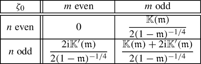
It remains to determine the phase shift $\zeta _0$ by ensuring that the correct “sign” of pole or zero of $f(\zeta -\zeta _0)$ lies at $\zeta =0$. Here the results depend not only on the sector of the parameter space shown in Fig. 1 but also on the parity of the indices (m, n) used to parametrize the allowed values of $(\Theta _0,\Theta _\infty )$. The results are as follows.

• Let $\kappa <-1$ and take $\mathfrak {m}\in (0,1)$ as in (D.4). If $(\Theta _{0,\textrm{F}}^{[1]}(m,n),\Theta _{\infty ,\textrm{F}}^{[1]}(m,n))\in \Lambda _\textrm{F}^{[1]-}$ (for either family $\textrm{F}=\textrm{gH}$ or $\textrm{F}=\textrm{gO}$), then $\zeta _0$ is given by

  

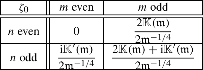
  If instead $(\Theta _{0,\textrm{gO}}^{[2]}(m,n),\Theta _{\infty ,\textrm{gO}}^{[2]}(m,n))\in \Lambda _\textrm{gO}^{[2]+}$, then $\zeta _0$ is given by

  

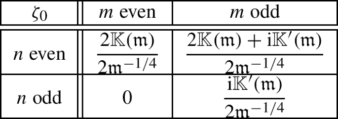
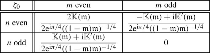
• Let $\kappa >1$ and take $\mathfrak {m}\in (0,1)$ as in (D.5). If $(\Theta _{0,\textrm{gO}}^{[1]}(m,n),\Theta _{\infty ,\textrm{gO}}^{[1]}(m,n))\in \Lambda _\textrm{gO}^{[1]+}$, then $\zeta _0$ is given by

  

  If instead $(\Theta _{0,\textrm{F}}^{[2]}(m,n),\Theta _{\infty ,\textrm{F}}^{[2]}(m,n))\in \Lambda _\textrm{F}^{[2]-}$ (for either family $\textrm{F}=\textrm{gH}$ or $\textrm{F}=\textrm{gO}$), then $\zeta _0$ is given by

  

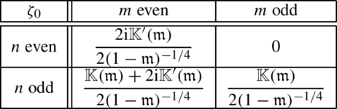
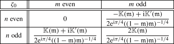
• Let $\kappa \in (-1,1)$ and take $\kappa \in \mathbb {C}$ as in (D.6). If $(\Theta _{0,\textrm{F}}^{[3]}(m,n),\Theta _{\infty ,\textrm{F}}^{[3]}(m,n))\in \Lambda _\textrm{F}^{[3]+}$ (for either family $\textrm{F}=\textrm{gH}$ or $\textrm{F}=\textrm{gO}$), then $\zeta _0$ is given by

  

  If instead $(\Theta _{0,\textrm{gO}}^{[3]}(m,n),\Theta _{\infty ,\textrm{gO}}^{[3]}(m,n))\in \Lambda _\textrm{gO}^{[3]-}$, then $\zeta _0$ is given by

  

These results are consistent in the gH case with [46, Corollary 1], a rigorous result describing the zeros of $H_{m,n}(x)$ near the origin as a locally regular lattice with spacings determined from complete elliptic integrals.

If we use the approach (ii) described in Sect. 1.4 in the discussion following Remark 4 in which a rational solution of Painlevé-IV is approximated locally near a given point $\mu$ by an exact elliptic function of $\zeta$ with a uniform lattice of poles and zeros, then we can easily use the knowledge of $\zeta _0$ detailed above to illustrate the attraction of the actual poles and zeros to the uniform lattice for the case $\mu =0$. This is shown for some gH rational solutions of types 1–3 in Figs. 36, 37, and 38.

Fig. 36

Zeros and poles of $u^{[1]}_\textrm{gH}(T^{-1/2}\zeta ;m,n)$ in the $\zeta$-plane (bold colors) and their large-T elliptic function approximations (faded colors). Cyan circles: zeros with positive derivative. Blue circles: zeros with negative derivative. Magenta dots: poles with positive residue. Grey dots: poles with negative residue. For the point at $\zeta =0$ which corresponds to $x=0$, these match the theoretical predictions of Proposition 13 (Color figure online)

Fig. 37

As in Fig. 36 but for $u^{[2]}_\textrm{gH}(T^{-1/2}\zeta ;m,n)$ (Color figure online)

Fig. 38

As in Figs. 36 and 37 but for $u^{[3]}_\textrm{gH}(T^{-1/2}\zeta ;m,n)$ (Color figure online)

These plots show the characteristic feature that since $\mu$ is fixed, the approximation for given $\zeta$ improves as the indices (m, n) increase, while for given (m, n) large it becomes less accurate as $|\zeta |$ grows. This is to be expected whether or not the approximation is exact at $\zeta =0$.

Appendix E. Diagrams and Tables for Steepest-Descent Analysis on Boutroux Domains

Here we gather z-plane diagrams and tables referred to in Sect. 7. In all plots gray shading means $\textrm{Re}(h(z))<0$ and white background means $\textrm{Re}(h(z))>0$.

1.1 E.1. The gO Case with $\mu \in \mathcal {B}_\square (\kappa )$ and $s=1$

Here we use representative values of $\mu =0$ and $\kappa =0$ (Fig. 39, Table 7).

Fig. 39

Diagrams for the gO case with $\mu \in \mathcal {B}_\square (\kappa )$ and $s=1$ (Color figure online)

Table 7 Inner parametrix data for the gO case with $\mu \in \mathcal {B}_\square (\kappa )$ and $s=1$

1.2 E.2. The gH Case with $\mu \in \mathcal {B}_\square (\kappa )$ and $s=1$

Here we use representative values of $\mu =0$ and $\kappa =0$ (Fig. 40, Table 8).

Fig. 40

Diagrams for the (only) gH case with $\mu \in \mathcal {B}_\square (\kappa )$ and $s=1$ (Color figure online)

Table 8 Inner parametrix data for the (only) gH case with $\mu \in \mathcal {B}_\square (\kappa )$ and $s=1$

1.3 E.3. The gO Case with $\mu \in \mathcal {B}_\square (\kappa )$ and $s=-1$

Here we use representative values of $\mu =0$ and $\kappa =0$ (Fig. 41, Table 9).

Fig. 41

Diagrams for the gO case with $\mu \in \mathcal {B}_\square (\kappa )$ and $s=-1$ (Color figure online)

Table 9 Inner parametrix data for the gO case with $\mu \in \mathcal {B}_\square (\kappa )$ and $s=-1$

1.4 E.4. The gO Case with $\mu \in \mathcal {B}_\vartriangleright (\kappa )$ and $s=1$

Here we use representative values of $\mu =1.3$ and $\kappa =0$ (Fig. 42, Table 10).

Fig. 42

Diagrams for the gO case with $\mu \in \mathcal {B}_\vartriangleright (\kappa )$ and $s=1$ (Color figure online)

Table 10 Inner parametrix data for the gO case with $\mu \in \mathcal {B}_\vartriangleright (\kappa )$ and $s=1$

1.5 E.5. The gO Case with $\mu \in \mathcal {B}_\vartriangleright (\kappa )$ and $s=-1$

Here we use representative values of $\mu =1.3$ and $\kappa =0$ (Fig. 43, Table 11).

Fig. 43

Diagrams for the gO case with $\mu \in \mathcal {B}_\vartriangleright (\kappa )$ and $s=-1$ (Color figure online)

Table 11 Inner parametrix data for the gO case with $\mu \in \mathcal {B}_\vartriangleright (\kappa )$ and $s=-1$

1.6 E.6. The gO Case with $\mu \in \mathcal {B}_\vartriangle (\kappa )$ and $s=1$

Here we use representative values of $\mu =1.3\textrm{i}$ and $\kappa =0$ (Fig. 44, Table 12).

Fig. 44

Diagrams for the gO case with $\mu \in \mathcal {B}_\vartriangle (\kappa )$ and $s=1$ (Color figure online)

Table 12 Inner parametrix data for the gO case with $\mu \in \mathcal {B}_\vartriangle (\kappa )$ and $s=1$

1.7 E.7. The gO Case with $\mu \in \mathcal {B}_\vartriangle (\kappa )$ and $s=-1$

Here we use representative values of $\mu =1.3\textrm{i}$ and $\kappa =0$ (Fig. 45 and Table 13).

Fig. 45

Diagrams for the gO case with $\mu \in \mathcal {B}_\vartriangle (\kappa )$ and $s=-1$ (Color figure online)

Table 13 Inner parametrix data for the gO case with $\mu \in \mathcal {B}_\vartriangle (\kappa )$ and $s=-1$

Appendix F. User’s Guide: Approximating Rational Solutions on Boutroux Domains

The approximation most directly adapted to our analysis of Riemann–Hilbert Problem 1 in Sect. 3.1 is that of the rational functions $u^{[3]}_\textrm{gO}(x;m,n)$ and $u^{[3]}_\textrm{gH}(x;m,n)$. The basic approximation formula for these functions reads:

(F.1)

Assuming that $\chi =-\textrm{sgn}(\ln |f(\zeta -\zeta _0)|)$, the error term is uniform for bounded $\zeta$ and for $\mu$ in a compact subset of the selected Boutroux domain $\mathcal {B}$. Computing the leading term consists of the following steps.

• (1) Define the parameters $T>0$, $s=\pm 1$, and $\kappa \in (-1,1)$ in terms of (m, n) by (4.3) (resp., by (4.4)) for the gH family (resp., for the gO family).

• (2) Select a Boutroux domain $\mathcal {B}=\mathcal {B}_\vartriangleright (\kappa )$, $\mathcal {B}=\mathcal {B}_\vartriangle (\kappa )$ (both for the gO family only), or $\mathcal {B}=\mathcal {B}_\square (\kappa )$, and ensure that $\mu \in \mathcal {B}$ (the boundaries of the domains can be numerically computed given $\kappa$ using (1.22); see also Appendix G.

• (3) Using numerical root finding and continuation methods informed by the discussion in Sect. 4.4, determine the value of $E=E(\mu ;\kappa )$ for which the Boutroux equations (4.23) hold.

• (4) With E determined, the polynomial P(z) given by (1.18) is now known. Find its roots $\alpha$, $\beta$, $\gamma$, and $\delta$ and order them according to the Stokes graph as illustrated in Figs. 39a–45a from Appendix E relevant for the family, Boutroux domain, and sign s under consideration (recall that while these figures are for special cases of the parameters, the abstract Stokes graph depends only on the selected Boutroux domain). Then using the contours $\ell _1$ and $\ell _2$ and branch cuts for R(z) illustrated in the same plots, numerically compute the real constants $R_1$ and $R_2$ given by (7.1) (one can use this computation as an opportunity to verify the accuracy of the determination of E, which should force the imaginary parts of $R_1$ and $R_2$ to vanish to machine precision).

• (5) Matching the topological representation of $\mathfrak {a}$ and $\mathfrak {b}$ cycles shown in Fig. 28 of Sect. 7.6 with the actual ordering of the points obtained in the previous step, and using the relationship (7.8), numerically calculate the constant c given in (7.13) and the constant $H_\omega$ given in (7.15). Then taking into account the value of $z_0$ given in terms of the well-defined branch points $\alpha$, $\beta$, $\gamma$, $\delta$ by (7.21), numerically evaluate the integrals a(0), $a(\infty )$, and $a(z_0)$ (see (7.17)). Using these, define the phase shifts $\mathfrak {z}_j^{\smash {[3]}}$ and $\mathfrak {p}^{\smash {[3]}}_j$, $j=1,2$, by (7.41).

• (6) Using Table 6 from Sect. 7.6 to determine the phases $C_\textrm{G}$ and $C_\textrm{B}$ relevant to the case at hand (noting also $\Theta _\infty =-\kappa T$), define the aggregate phase $\Psi$ by (7.26).

• (7) Recalling the definition (7.22) of $\vartheta (z)$ given $H_\omega$ (possibly implementing this definition using built-in function calls to Jacobi theta functions) and using $\mathcal {K}=\textrm{i}\pi +\tfrac{1}{2}H_\omega$, calculate the complex amplitude factor $\psi ^{[3]}_\textrm{F}(\mu )$ from (7.43). Then bring in $\Psi$ and the four phase shifts to finish the rest of the calculation using (F.1).

The other approximation proved by analyzing the same Riemann–Hilbert Problem applies to the rational functions $u_\textrm{gO}^{[1]}(x;m,n)$ and $u_\textrm{gH}^{[1]}(x;m,n)$, and it reads

$$\begin{aligned} \begin{aligned}&u_\textrm{F}^{[1]}\left( |\Theta _{0,\textrm{F}}^{[1]}(m,n)|^{1/2}\widehat{\mu }+|\Theta _{0,\textrm{F}}^{[1]}(m,n)|^{-1/2}\widehat{\zeta };m,n\right) \\&\quad =|\Theta _{0,\textrm{F}}^{[1]}(m,n)|^{1/2}\left( f(\zeta -\zeta _0)^\chi +\mathcal {O}\left( |\Theta _{0,\textrm{F}}^{[1]}(m,n)|^{-1}\right) \right) ^\chi ,\\&f(\widehat{\zeta }-\widehat{\zeta _0})={\breve{U}}^{[1]}_\textrm{F}(\widehat{\zeta };\widehat{\mu }):=\psi _\textrm{F}^{[1]}(\widehat{\mu })\frac{\vartheta (\mathcal {K}-\textrm{i}(\Psi -\mathfrak {z}_1^{[1]}))\vartheta (\mathcal {K}-\textrm{i}(\Psi -\mathfrak {z}_2^{[1]}))}{\vartheta (\mathcal {K}-\textrm{i}(\Psi -\mathfrak {p}_1^{[1]}))\vartheta (\mathcal {K}-\textrm{i}(\Psi -\mathfrak {p}_2^{[1]}))}. \end{aligned} \end{aligned}$$

(F.2)

Again taking $\chi =-\textrm{sgn}(\ln |f(\widehat{\zeta }-\widehat{\zeta _0})|)$, the error term is uniform for bounded $\widehat{\zeta }$ and for $\widehat{\mu }$ in a compact subset of the chosen Boutroux domain $\mathcal {B}$. To compute the leading term, we modify the above steps as follows.

• (1) Define the parameters $T>0$, $s=\pm 1$, and $\kappa \in (-1,1)$ in terms of (m, n) by (4.6) (resp., by (4.8)) for the gH family (resp., for the gO family). These are not directly related to the “native” parameters $\Theta _{0,\textrm{F}}^{[1]}(m,n)$ and $\Theta _{\infty ,\textrm{F}}^{[1]}(m,n)$, but they are the correct values to use for the remaining steps of the calculation. From the given values of the variables $\widehat{\zeta }$ and $\widehat{\mu }$, define scaled versions needed for the subsequent steps by setting

  $$\begin{aligned} \zeta :=\sqrt{\frac{2}{1-s\kappa }}\widehat{\zeta }\quad \text {and}\quad \mu :=\sqrt{\frac{1-s\kappa }{2}}\widehat{\mu }. \end{aligned}$$

• (2) As above.

• (3) As above.

• (4) As above.

• (5) As above, but instead calculate the phase shifts $\mathfrak {z}_j^{\smash {[1]}}$ and $\mathfrak {p}_j^{\smash {[1]}}$ from (7.47).

• (6) As above for the indicated parameters.

• (7) As above for the indicated parameters, but now define the complex amplitude $\psi _\textrm{F}^{[1]}(\widehat{\mu })=\textrm{e}^{\textrm{i}(\mathfrak {z}_1^{[1]}-\mathfrak {p}_2^{[1]})}M$ in terms of M given in (7.48), and finish the calculation using (F.2).

We do not obtain any approximations for the rational solutions $u_\textrm{gO}^{[2]}(x;m,n)$ or $u_\textrm{gH}^{[2]}(x;m,n)$ directly from analysis of Riemann–Hilbert Problem 1, but we can apply the exact symmetry (2.2) to obtain the following result.

$$\begin{aligned} \begin{aligned}&u_\textrm{F}^{[2]}\left( |\Theta _{0,\textrm{F}}^{[2]}(m,n)|^{1/2}\mu +|\Theta _{0,\textrm{F}}^{[2]}(m,n)|^{-1/2}\zeta ;m,n\right) \\&\quad =|\Theta _{0,\textrm{F}}^{[2]}(m,n)|^{1/2}\left( f(\zeta -\zeta _0)^\chi +\mathcal {O}\left( |\Theta _{0,\textrm{F}}^{[2]}(m,n)|^{-1}\right) \right) ^\chi ,\\&f(\zeta -\zeta _0)={\breve{U}}^{[2]}_\textrm{F}(\zeta ;\mu ):=\textrm{i}{\breve{U}}^{[1]}_\textrm{F}(-\textrm{i}\zeta ;-\textrm{i}\mu ). \end{aligned} \end{aligned}$$

Taking $\chi =-\textrm{sgn}(\ln |f(\zeta -\zeta _0)|)$, this formula is also uniformly valid for bounded $\zeta$ and $\mu$ in a compact subset of the chosen Boutroux domain $\mathcal {B}$. The leading term can obviously be computed by adapting the above procedure to variables rotated by $-\textrm{i}$ in the complex plane.

Appendix G.User’s Guide: Practical Computation of Boundary Curves

In this appendix, we provide further details about how (1.22) can be used practically to compute the boundary curves. An antiderivative of the integrand in (1.22) is

$$\begin{aligned} \begin{aligned}&\int (f-\gamma )\sqrt{(f-\alpha )(f-\beta )}\,\frac{\textrm{d}f}{f} = \frac{1}{4}\sqrt{(f-\alpha )(f-\beta )}(2f-\alpha -\beta -4\gamma ) \\&\qquad {}- \frac{1}{8}((\alpha +\beta )^2-4(\alpha +\beta )\gamma -4\alpha \beta )\log \left( \frac{f-\alpha +\sqrt{(f-\alpha )(f-\beta )}}{f-\alpha -\sqrt{(f-\alpha )(f-\beta )}}\right) \\&\qquad {}-\sqrt{\alpha }\sqrt{\beta }\gamma \log \left( \frac{\sqrt{\beta }(f-\alpha )+\sqrt{\alpha }\sqrt{(f-\alpha )(f-\beta )}}{\sqrt{\beta }(f-\alpha )-\sqrt{\alpha }\sqrt{(f-\alpha )(f-\beta )}}\right) . \end{aligned} \end{aligned}$$

Since $\alpha$ and $\beta$ are the roots of the quadratic (1.21), the identities $\alpha \beta \gamma ^2=16$ and $\alpha +\beta =-4\mu -2\gamma$ both hold. Using these as well as the quartic equation (1.15) satisfied by $\gamma =U_0$, the coefficient of the first logarithm is simply

$$\begin{aligned} - \frac{1}{8}((\alpha +\beta )^2-4(\alpha +\beta )\gamma -4\alpha \beta )=4\kappa \in \mathbb {R}. \end{aligned}$$

Likewise, the coefficient of the second logarithm is $-\sqrt{\alpha }\sqrt{\beta }\gamma = \pm 4\in \mathbb {R}$. Furthermore, evaluating at the limits of integration $f=\gamma$ and (by taking a limit) $f=\alpha$ and taking the real part gives

$$\begin{aligned} \begin{aligned}&\textrm{Re}\left( \int _{\alpha }^\gamma (f-\gamma )\sqrt{(f-\alpha )(f-\beta )}\,\frac{\textrm{d}f}{f}\right) = -\frac{1}{4}\textrm{Re}\left( \sqrt{(\gamma -\alpha )(\gamma -\beta )}(\alpha +\beta +2\gamma )\right) \\&\qquad {}+4\kappa \log \left| \frac{\gamma -\alpha +\sqrt{(\gamma -\alpha )(\gamma -\beta )}}{\gamma -\alpha -\sqrt{(\gamma -\alpha )(\gamma -\beta )}}\right| \\&\qquad {}-\sqrt{\alpha }\sqrt{\beta }\gamma \log \left| \frac{\sqrt{\beta }(\gamma -\alpha )+\sqrt{\alpha }\sqrt{(\gamma -\alpha )(\gamma -\beta )}}{\sqrt{\beta }(\gamma -\alpha )-\sqrt{\alpha }\sqrt{(\gamma -\alpha )(\gamma -\beta )}}\right| . \end{aligned} \end{aligned}$$

This formula is invariant under permutation of $(\alpha ,\beta )$, and the last term does not depend on the choice of signs in the square roots $\sqrt{\alpha }$ and $\sqrt{\beta }$. Although the whole formula changes sign if $\sqrt{(\gamma -\alpha )(\gamma -\beta )}$ changes sign, this is irrelevant in identifying the zero set as required in the condition (1.22). At this point, we can use the fact that $\gamma =U_0$ is a root of the quartic equation (1.15), so it becomes locally one of four functions of $\mu$ parametrized by $\kappa$, and then $\alpha$ and $\beta$ are in turn determined (up to permutation) as functions of $\mu$ with parameter $\kappa$ via the quadratic equation (1.21). Thus on each of the four sheets of the solution of (1.15) over a given domain in the $\mu$-plane, the condition (1.22) defines a system of arcs that are the zeros of a harmonic function of $\mu$. By combining the above explicit formula with the well-known explicit solution of the quartic equation (1.15) for $\gamma =U_0$ in terms of radicals and the subsequent use of the quadratic formula to solve (1.21) for $\alpha$ and $\beta$ one converts (1.22) into an explicit harmonic function of $\mu$ whose zero locus can be found using standard computational software.

Appendix H. Alternate Approach to Rational Solutions of Types 1 and 2

The basic approach we have followed in this paper is to use the fact that the Painlevé-IV rational solutions of type 1, which correspond to values of $\kappa$ outside of the basic interval $(-1,1)$, can be extracted via the formula (3.2) for from Riemann–Hilbert Problem 1 in Sect. 3.1 formulated for the rational solutions of type 3, which correspond instead to $\kappa \in (-1,1)$. Of course another approach to the rational solutions of type 1 (and also type 2) is to represent these solutions as u(x) instead of in (3.2) and solve Riemann–Hilbert Problem 1 for parameters covering all lattice points far from the origin in Fig. 1. The latter approach avoids the complication of the changes of variables associated with the Bäcklund transformation , but it leads to many additional cases for matrix factorizations and parametrix constructions, as one must consider spectral curves for $\kappa <-1$ and $\kappa >1$, as well as for $\kappa \in (-1,1)$.

1.1 H.1. Monodromy Data for gH Rational Solutions of Types 1 and 2

One further difficulty of this alternate approach in the gH case is that the rational solutions for $(\Theta _0,\Theta _\infty )\in \Lambda _\textrm{gH}^{[1]-}\cup \Lambda _\textrm{gH}^{[2]-}$ cannot be obtained from those for $(\Theta _0,\Theta _\infty )\in \Lambda _\textrm{gH}^{[3]+}$ by means of isomonodromic transformations, so to treat these rational solutions as functions u(x) in Riemann–Hilbert Problem 1 it is necessary to repeat the procedure of Sect. 3.6 for a seed solution with parameters in $\Lambda _\textrm{gH}^{[1]-}$. Note that this issue does not arise for the gO solutions as the entire lattice $\Lambda _\textrm{gO}$ is spanned by isomonodromic transformations.

Applying the transformation to the seed solution $u(x)=-2x$ for $(\Theta _0,\Theta _\infty )=(\tfrac{1}{2},\tfrac{1}{2})\in \Lambda _\textrm{gH}^{[3]+}$, we obtain the solution $u(x)=x^{-1}$ for parameters $(\Theta _0,\Theta _\infty )=(-\tfrac{1}{2},\tfrac{3}{2})\in \Lambda _\textrm{gH}^{[1]-}$. Without loss of generality taking the corresponding solution of (3.7) to be $y(x)=x^{-1}\exp (-x^2)$, and noting that from (3.8) we get $z(x)=1+\tfrac{1}{2}x^{-2}$, the Lax pair matrix coefficients $\varvec{\Lambda }_0(x)$, $\varvec{\Lambda }_1(x)$, and $\textbf{X}_0(x)$ defined in (3.10)–(3.11) become

$$\begin{aligned} \varvec{\Lambda }_0(x)= & {} \begin{pmatrix} x &{} x^{-1}\textrm{e}^{-x^2}\\ \textrm{e}^{x^2}(x^{-1}-2x) &{} -x\end{pmatrix},\; \\ \varvec{\Lambda }_1(x)= & {} \begin{pmatrix} -\tfrac{1}{2}(1+x^{-2}) &{} -\tfrac{1}{2}x^{-2}\textrm{e}^{-x^2}\\ \textrm{e}^{x^2}(1+\tfrac{1}{2}x^{-2}) &{} \tfrac{1}{2}(1+x^{-2})\end{pmatrix},\;\\ \textbf{X}_0(x)= & {} \varvec{\Lambda }_0(x)-x\sigma _3. \end{aligned}$$

Following the same strategy we have used twice before, we look first for solutions of $\varvec{\Psi }_x=\textbf{X}\varvec{\Psi }$, and some experimentation shows that a particular solution is given in closed form by $\Psi _{1j}=x^{-1}\exp (-x^2-x\lambda )$ and $\Psi _{2j}=-(2x+2\lambda +x^{-1})\exp (-x\lambda )$. Applying reduction of order to obtain the general solution, and then determining the dependence of constants of integration on $\lambda$ so that the other Lax equation $\varvec{\Psi }_\lambda =\varvec{\Lambda \Psi }$ holds, we obtain the following analogue of Lemma 2 and Lemma 3.

Lemma 21

Fix a simply connected domain $D\subset \mathbb {C}\setminus \{0\}$ and a branch of $\lambda ^{1/2}$ analytic on D. Let $\Theta _0=-\tfrac{1}{2}$ and $\Theta _\infty =\tfrac{3}{2}$, and consider the exact solution $u(x)=x^{-1}$ of the corresponding Painlevé-IV equation (1.1). If $y(x)=x^{-1}\exp (-x^2)$, then the Lax pair equations (3.9) are simultaneously solvable for all $(\lambda ,x)\in D\times (\mathbb {C}\setminus \{0\})$, and every simultaneous solution matrix has the form

$$\begin{aligned} \varvec{\Psi }(\lambda ,x)= & {} \frac{\lambda ^{1/2}}{x}\begin{pmatrix} \textrm{e}^{-x^2} &{} \frac{1}{2}\lambda ^{-1}-F(x+\lambda )\\ -(2x^2+2x\lambda +1) &{} [-(x+\frac{1}{2}\lambda ^{-1})+(2x^2+2x\lambda +1)F(x+\lambda )]\textrm{e}^{x^2} \end{pmatrix}\nonumber \\{} & {} \cdot \exp (-(\tfrac{1}{2}\lambda ^2+x\lambda )\sigma _3) \textbf{C}, \end{aligned}$$

(H.1)

where $F(z):=\exp (-z^2)\int _0^z\exp (t^2)\,\textrm{d}t$ denotes Dawson’s integral [53, §7.2(ii)] and $\textbf{C}$ is a matrix independent of both x and $\lambda$.

Absence of logarithms again indicates that although the Fuchsian singularity of $\varvec{\Psi }_\lambda =\varvec{\Lambda \Psi }$ is resonant, it is also apparent, so it is possible to choose $\textbf{C}=\textbf{C}^{(0)}$ to define a solution for $|\lambda |<1$ to satisfy (3.13). For solutions defined to satisfy (3.12) in the four Stokes sectors we determine $\textbf{C}=\textbf{C}^{(\infty )}_j$, $j=1,\dots ,4$ by asymptotic analysis of the general solution given in Lemma 21 for large $\lambda$. The results are

$$\begin{aligned} \textbf{C}_2^{(\infty )}=\textbf{C}_3^{(\infty )}=\begin{pmatrix} \textrm{i}\sqrt{\pi } &{} -\tfrac{1}{2}\\ 2 &{} 0\end{pmatrix}\quad \text {and}\quad \textbf{C}_1^{(\infty )}=\textbf{C}_4^{(\infty )}=\begin{pmatrix} -\textrm{i}\sqrt{\pi } &{} -\tfrac{1}{2}\\ 2 &{} 0\end{pmatrix}. \end{aligned}$$

Therefore, there is no Stokes phenomenon between sectors $S_2$ and $S_3$ or between $S_4$ and $S_1$ (i.e., upon crossing the imaginary Stokes rays), and the corresponding Stokes matrices $\textbf{V}_{2,3}=\textbf{V}_{4,1}=\mathbb {I}$ defined in (3.15) and (3.17) respectively are trivial. On the other hand, from (3.14) and (3.16) we get

$$\begin{aligned} \textbf{V}_{2,1}=\begin{pmatrix} 1 &{} 0\\ -4\textrm{i}\sqrt{\pi } &{} 1 \end{pmatrix}\quad \text {and}\quad \textbf{V}_{4,3} = \begin{pmatrix} -1 &{} 0\\ -4\textrm{i}\sqrt{\pi } &{} -1 \end{pmatrix}. \end{aligned}$$

Therefore, unlike the gH rationals in the parameter lattice $\Lambda _\textrm{gH}^{[3]+}$, the rationals in the parameter lattice $\Lambda _\textrm{gH}^{[1]-}$ have nontrivial Stokes matrices on the real rays. Similar analysis shows that gH rational solutions in the parameter lattice $\Lambda _\textrm{gH}^{[2]-}$ have instead nontrivial Stokes phenomenon (only) across the imaginary rays.

Fig. 46

Critical v-trajectories of $h'(z)^2\,\textrm{d}z^2$ emanating from (for generic $\mu$) simple roots of P(z) for $\kappa =3$ for the gH family. The same topological structure holds for $\kappa >1$. Counterclockwise from top left: $\mu =2\textrm{i}$, $\mu \approx 1.45\textrm{i}$, $\mu =0.7\textrm{i}$, $\mu =0$, $\mu =0.7$, $\mu \approx 1.45$, $\mu =2$, $\mu =2+0.7\textrm{i}$, $\mu =2+1.45\textrm{i}$, $\mu =2+2\textrm{i}$, $\mu =1.45+2\textrm{i}$, $\mu =0.7+2\textrm{i}$. Inset: Boundary of $\mathcal {B}_\square (3)$ in the $\mu$-plane. The $\mu$-values corresponding to different trajectory plots are indicated by red dots (Color figure online)

Fig. 47

Critical v-trajectories of $h'(z)^2\,\textrm{d}z^2$ emanating from simple roots of P(z) for $\kappa =3$ for the gO family (for nongeneric values of $\mu$ on boundary curves we show all critical trajectories). The same topological structure holds for $\kappa >1$. Counterclockwise from top left: $\mu \approx 4.19698\textrm{i}$, $\mu =3\textrm{i}$, $\mu \approx 1.45\textrm{i}$, $\mu =0.7\textrm{i}$, $\mu =0$, $\mu =0.7$, $\mu \approx 1.45$, $\mu =3$, $\mu \approx 4.19698$, $\mu =4.2+0.7\textrm{i}$, $\mu =4.2+1.45\textrm{i}$, $\mu =4.2+3\textrm{i}$, $\mu =4.2+4.2\textrm{i}$, $\mu =3+4.2\textrm{i}$, $\mu =1.45+4.2\textrm{i}$, $\mu =0.7+4.2\textrm{i}$. Inset: Boundaries of the regions $\mathcal {B}_\square (3)$, $\pm \mathcal {B}_\vartriangleright (3)$, and $\pm \mathcal {B}_\vartriangle (3)$ in the $\mu$-plane. The $\mu$-values corresponding to different trajectory plots are indicated by red dots

1.2 H.2. Critical v-Trajectories of $h'(z)^2\,\textrm{d}z^2$ for $|\kappa |>1$

The main idea of the asymptotic analysis of Riemann–Hilbert Problem 1 in all cases is to use the landscape of $\textrm{Re}(h(z))$ in the z-plane, where as explained in Sect. 4.3h(z) is associated to the spectral curve for the polynomial $P(z)=P(z;\mu ,\kappa ,E)$ defined in (1.18). The type-1 solutions correspond to values of $\kappa$ outside of the interval $(-1,1)$. Just to give a flavor of the differences that can arise for $|\kappa |>1$, in Figs. 46 and 47 we present the analogues of Figs. 16 and 17 in Sect. 4.3 in which we display the critical v-trajectories of the quadratic differential $h'(z)^2\,\textrm{d}z^2$ emanating from (generically) simple roots of the quartic P(z).

References

Adler, V.É.: Nonlinear chains and Painlevé equations. Phys. D 73, 335–351 (1994)
Airault, H.: Rational solutions of Painlevé equations. Stud. Appl. Math. 61, 31–53 (1979)
Aratyn, H., Gomes, J.F., Zimmerman, A.H.: Darboux-Bäcklund transformations and rational solutions of the Painlevé IV equation. AIP Conf. Proc. 1212, 146–153 (2010)
Balogh, F., Bertola, M., Bothner, T.: Hankel determinant approach to generalized Vorob’ev–Yablonski polynomials and their roots. Constr. Approx. 44, 417–453 (2016)
Bassom, A.P., Clarkson, P.A., Hicks, A.C.: Bäcklund transformations and solution hierarchies for the fourth Painlevé equation. Stud. Appl. Math. 95, 1–71 (1995)
Bassom, A.P., Clarkson, P.A., Hicks, A.C.: On the application of solutions of the fourth Painlevé equation to various physically motivated nonlinear partial differential equations. Adv. Differ. Equ. 1, 175–198 (1996)
Bertola, M., Bothner, T.: Zeros of large degree Vorob’ev-Yablonski polynomials via a Hankel determinant identity. Int. Math. Res. Not. 2015, 9330–9399 (2015)
Bertola, M., Lee, S.: First colonization of a spectral outpost in random matrix theory. Constr. Approx. 30, 225–263 (2009)
Bertola, M., Tovbis, A.: Universality in the profile of the semiclassical limit solutions to the focusing nonlinear Schrödinger equation at the first breaking curve. Int. Math. Res. Not. 2010, 2119–2167 (2010)
Bilman, D., Buckingham, R., Wang, D.: Far-field asymptotics for multiple-pole solitons in the large-order limit. J. Differ. Equ. 297, 320–369 (2021)
Boiti, M., Pempinelli, F.: Nonlinear Schrödinger equation, Bäcklund transformations and Painlevé transcendents. Nuovo Cim. 59B, 40–58 (1980)
Bothner, T., Miller, P.D.: Rational solutions of the Painlevé-III equation: large parameter asymptotics. Constr. Approx. 51, 123–224 (2020)
Bothner, T., Miller, P.D., Sheng, Y.: Rational solutions of the Painlevé-III equation. Stud. Appl. Math. 141, 626–679 (2018)
Boutroux, P.: Recherches sur les transcendantes de M. Painlevé et l’étude asymptotique des équations différentielles du second ordre. Ann. Sci. École Norm. Sup. 30, 255–375 (1913). (In French)
Buckingham, R.: Large-degree asymptotics of rational Painlevé-IV functions associated to generalized Hermite polynomials. Int. Math. Res. Not. IMRN 2018, rny172 (2018)
Buckingham, R., Miller, P.D.: The sine-Gordon equation in the semiclassical limit: critical behavior near a separatrix. J. Anal. Math. 118, 397–492 (2012)
Buckingham, R., Miller, P.D.: The sine-Gordon equation in the semiclassical limit: dynamics of fluxon condensates. Memoirs Amer. Math. Soc. 225, 1–136 (2013)
Buckingham, R., Miller, P.D.: Large-degree asymptotics of rational Painlevé-II functions: noncritical behaviour. Nonlinearity 27, 2489–2577 (2014)
Buckingham, R., Miller, P.D.: Large-degree asymptotics of rational Painlevé-II functions: critical behaviour. Nonlinearity 28, 1539–1596 (2015)
Chen, Y., Feigin, M.: Painlevé IV and degenerate Gaussian unitary ensembles. J. Phys. A 39, 12381–12393 (2006)
Clarkson, P.A.: The fourth Painlevé equation and associated special polynomials. J. Math. Phys. 44, 5350–5374 (2003)
Clarkson, P.A.: Special polynomials associated with rational solutions of the defocusing nonlinear Schrödinger equation and the fourth Painlevé equation. Eur. J. Appl. Math. 17, 293–322 (2006)
Clarkson, P.A.: Special polynomials associated with rational solutions of the Painlevé equations and applications to soliton equations. Comp. Meth. Func. Theory 6, 329–401 (2006)
Clarkson, P.A.: Rational solutions of the Boussinesq equation. Anal. Appl. (Singap.) 6, 349–369 (2008)
Clarkson, P.A.: Rational solutions of the classical Boussinesq system. Nonlinear Anal. Real World Appl. 10, 3360–3371 (2009)
Clarkson, P.A.: Vortices and polynomials. Stud. Appl. Math. 123, 37–62 (2009)
Clarkson, P.A., Thomas, B.: Special polynomials and exact solutions of the dispersive water wave and modified Boussinesq equations. In: Proceedings of Group Analysis of Differential Equations and Integrable Systems IV, pp. 62–76 (2009)
Dai, D., Kuijlaars, A.: Painlevé IV asymptotics for orthogonal polynomials with respect to a modified Laguerre weight. Stud. Appl. Math. 122, 29–83 (2009)
Deift, P., Venakides, S., Zhou, X.: The collisionless shock region for the long-time behavior of solutions of the KdV equation. Comm. Pure Appl. Math. 47, 199–206 (1994)
Deift, P., Zhou, X.: A steepest descent method for oscillatory Riemann–Hilbert problems: asymptotics for the mKdV equation. Ann. Math. 137, 295–368 (1993)
Dubrovin, B.A.: Theta functions and non-linear equations. Russian Math. Surveys 36, 11–92 (1981)
Fokas, A.S., Grammaticos, B., Ramani, A.: From continuous to discrete Painlevé equations. J. Math. Anal. Appl. 180, 342–360 (1993)
Fokas, A.S., Its, A.R., Kapaev, A.A., Yu, V.: Novokshenov, Painlevé Transcendents. The Riemann–Hilbert Approach, AMS Mathematical Surveys and Mongraphs 128, Amer. Math. Soc., Providence (2006)
Fokas, A.S., Its, A.R., Kitaev, A.V.: Discrete Painlevé equations and their appearance in quantum gravity. Comm. Math. Phys. 142, 313–344 (1991)
Fokas, A.S., Muğan, U., Ablowitz, M.J.: A method of linearization for Painlevé equations: Painlevé IV, V. Physica D 30, 247–283 (1988)
Forrester, P., Witte, N.: Application of the \(\tau \)-function theory of Painlevé equations to random matrices: PIV, PII and the GUE. Comm. Math. Phys. 219, 357–398 (2001)
Gromak, V.: On the theory of the fourth Painlevé equation. Differentsialnye Uravneniya 23, 760–768 (1987). (In Russian)
Its, A.R.: Asymptotic behavior of the solutions to the nonlinear Schrödinger equation, and isomonodromic deformations of systems of linear differential equations. Dokl. Akad. Nauk SSSR 261, 14–18 (1981). (In Russian)
Jenkins, J.A.: Univalent Functions and Conformal Mapping. Springer, Berlin (1958)
Jimbo, M., Miwa, T.: Monodromy preserving deformation of linear ordinary differential equations with rational coefficients. II. Physica D 2, 407–448 (1981)
Joshi, N., Liu, E.: Asymptotic behaviours given by elliptic functions in \({\rm P}_I\)-\({\rm P}_V\). Nonlinearity 31, 3626–3747 (2018)
Kajiwara, K., Ohta, Y.: Determinant structure of the rational solutions for the Painlevé-IV equation. J. Phys. A 31, 2431–2446 (1998)
Lukashevich, N.: The theory of Painlevé’s fourth equation. Differensialnye Uravnenija 3, 771–780 (1967). (In Russian)
Marikhin, V., Shabat, A., Boiti, M., Pempinelli, F.: Self-similar solutions of equations of the nonlinear Schrödinger type. J. Exp. Theor. Phys. 90, 553–561: Translation of Zh. Eksper. Teoret. Fiz. 117, 634–643 (2000). (In Russian)
Marquette, I., Quesne, C.: Connection between quantum systems involving the fourth Painlevé transcendent and \(k\)-step rational extensions of the harmonic oscillator related to Hermite exceptional orthogonal polynomial. J. Math. Phys. 57, 052101 (2006)
Masoero, D., Roffelsen, P.: Poles of Painlevé IV rationals and their distribution. SIGMA Symmetry Integrability Geom. Methods Appl. 14, paper no 002 (2018)
Masoero, D., Roffelsen, P.: Roots of generalised Hermite polynomials when both parameters are large. Nonlinearity 34, 1663–1732 (2021)
Masoero, D., Roffelsen, P.: Private communication (2020)
Miller, P.D.: On the increasing tritronquée solutions of the Painlevé-II equation. SIGMA Symmetry Integrability Geom. Methods Appl. 14, paper no. 125 (2018)
Miller, P.D., Sheng, Y.: Rational solutions of the Painlevé-II equation revisited. SIGMA Symmetry Integrability Geom. Methods Appl. 13, paper no. 065 (2017)
Muğan, U., Fokas, A.S.: Schlesinger transformations of Painlevé II-V. J. Math. Phys. 33, 2031–2045 (1992)
Murata, Y.: Rational solutions of the second and the fourth Painlevé equations. Funkcial. Ekvac. 28, 1–32 (1985)
NIST Digital Library of Mathematical Functions. http://dlmf.nist.gov/, Release 1.0.27 of 2020-06-15. Online companion to [58]
Noumi, M., Yamada, Y.: Symmetries in the fourth Painlevé equation and Okamoto polynomials. Nagoya Math. J. 153, 53–86 (1999)
Yu, V., Novokshenov and A. A. Shchelkonogov,: Double scaling limit in the Painlevé IV equation and asymptotics of the Okamoto polynomials. Amer. Math. Soc. Trans. 233, 199–210 (2014)
Yu, V., Novokshenov and A. A. Shchelkonogov,: Distribution of zeroes to generalized Hermite polynomials. Ufa Math. J. 7, 54–66 (2015)
Okamoto, K.: Studies on the Painlevé equations III. Second and fourth Painlevé equations, P\(_{\rm II}\) and P\(_{\rm IV}\). Math. Ann. 275, 221–255 (1986)
Olver, F.W.J., Lozier, D.W., Boisvert, R.F., Clark, C.W. (Eds.) NIST Handbook of Mathematical Functions, Cambridge University Press, New York. Print companion to [53] (2010)
Osipov, V., Sommers, H., Zyczkowski, K.: Random Bures mixed states and the distribution of their purity. J. Phys. A 43, 055302 (2010)
Strebel, K.: Quadratic Differentials. Springer Verlag, Berlin (1984)
Van Assche, W.: Orthogonal Polynomials and Painlevé Equations, Australian Mathematical Society Lecture Series, vol. 27. Cambridge University Press, Cambridge (2018)
Acknowledgements
The authors thank Davide Masoero and Pieter Roffelsen for useful discussions and Guilherme Silva for information about trajectories of rational quadratic differentials and for suggesting the possibility of representing the arcs of the curves \(\partial \mathcal {E}_\textrm{gH}(\kappa )\) and \(\partial \mathcal {E}_\textrm{gO}(\kappa )\) in the \(\mu \)-plane in terms of such trajectories. Two anonymous referees also made valuable suggestions that improved the manuscript. R. J. Buckingham was supported by National Science Foundation (grants DMS-1615718 and DMS-2108019). P. D. Miller was supported by the National Science Foundation (grants DMS-1513054 and DMS-1812625).
Author information
Authors and Affiliations
Corresponding author
Additional information
Communicated by Walter Van Assche.
Publisher's Note
Springer Nature remains neutral with regard to jurisdictional claims in published maps and institutional affiliations.