
Abstract
Imaging through optically dense sprays is challenging due to the detection of multiple light scattering, which blurs the recorded images and limits visibility. Structured laser illumination planar imaging (SLIPI) is a technique that is capable of reducing the intensity contribution that stems from multiple scattering in a light sheet imaging configuration. The conventional SLIPI approach is based on recording three modulated sub-images successively, each having a different spatial phase, and has, therefore, been mostly used for temporally averaged imaging. To circumvent this limitation and image spray dynamics, ‘instantaneous’ two-phase (2p) and single-phase (1p) SLIPI approaches have recently been developed. The purpose of the work presented here is to compare these two approaches in terms of optical design, image post-processing routines, multiple scattering suppression ability, and spatial resolution. The two approaches are used to image a transient direct-injection spark-ignition ethanol spray, for both liquid laser-induced fluorescence and Mie scattering detection. The capabilities of the approaches for multiple scattering suppression and image formation have also been numerically modeled by means of Monte Carlo simulation. This article shows that both approaches efficiently suppress the contribution from multiple light scattering, providing images with an intensity profile close to the corresponding single scattering case. Experimentally, this suppression renders both an improvement in image contrast and the removal of undesired stray light components that could be interpreted as signal. However, while 2p-SLIPI preserves most of the initial spatial resolution, 1p-SLIPI results in a loss of spatial resolution, where high-frequency image information is not visible anymore. Thus, there is a trade-off between preserving the most detailed information of the spray structure—with 2p-SLIPI—and being able to record an SLIPI image from a single modulated image only—with 1p-SLIPI. The comparison and technical overview of these two methods presented in this paper can facilitate in selecting which approach is the most suitable for a given application for spray visualization.
1 Introduction
The atomization of liquid fuels, both in gas turbines and in internal combustion (IC) engines, aims at increasing the fuel surface area, thus, increasing momentum and energy transfer at the interface of liquid and gaseous phase (Lee and Abraham 2011). Finer atomization not only ensures a faster fuel/air mixing time but also leads to more uniform mixing with minimal wall-wetting. An adequate mixing is required to maintain a fuel-efficient and low-emission IC engine. An in-depth understanding of the atomization process requires a detailed investigation of transient phenomena such as the primary breakup of the liquid jets/sheets, the secondary breakup of large droplets and ligaments, as well as the transport and evaporation of formed droplets. Such investigations have, therefore, been, and do remain, important for both the gas turbine and the IC engine community. Several optical measurement techniques have been developed in the past for the characterization of spray systems (Fansler and Parrish 2015; Linne 2013). Phase Doppler interferometry (Bachalo and Houser 1984) and laser diffraction (Dodge et al. 1987) are among some of the most common techniques reported initially. With the great progress in both camera sensor technology and illumination sources over the past two decades, imaging techniques such as microscopic imaging (Crua et al. 2015), X-ray absorption imaging (Halls et al. 2014), ballistic imaging (Linne et al. 2009), optical connectivity (Charalampous et al. 2009), and a variety of laser sheet imaging techniques have been created and extensively used. One of the main benefits of laser sheet imaging—wherein only a thin plane is illuminated—is its versatility regarding which quantities it can extract: flow velocities using particle image velocimetry (PIV) (Adrian and Westerweel 2011; Westerweel et al. 2013), droplet Sauter mean diameter (SMD) using LIF/Mie ratio techniques (Le Gal et al. 1999; Domann and Hardalupas 2003), and spray temperatures using the ratio of two spectral bands from either laser-induced fluorescence (Bruchhausen et al. 2005; Vetrano et al. 2013) or phosphorescence (Brübach et al. 2006; Omrane et al. 2004) emissions. Nearly all quantitative imaging techniques are based on the single scattering approximation, which assumes that the detected photons have experienced only one scattering event prior to reaching the detector. However, this assumption remains only valid for a low number density of particles and/or when the total photon path length within the probed medium is short. Within optically dense media, the majority of photons are scattered multiple times, and therefore, the single scattering approximation is no longer valid. The SLIPI technique, standing for structured laser illumination planar imaging (Berrocal et al. 2008), that combines structured illumination (Neil et al. 1997) and laser sheet imaging, has proven to be a valuable approach for suppressing the contribution from multiple light scattering.
In SLIPI, the illuminating light sheet is modulated in space, either with a sinusoidal or square intensity pattern, rather than a homogeneous pattern. The purpose of this “line pattern” is to experimentally differentiate between light that has been directly and multiply scattered and to computationally remove the latter. This is achieved by shifting the line pattern one-third of the spatial period and recording a set of three modulated images (sub-images). From this data set, a final demodulated SLIPI image can be extracted, wherein the contribution from the multiply scattered light has been reduced (Berrocal et al. 2008). However, due to the need for recording three sub-images, SLIPI has been mostly used for temporally averaged measurements of spray quantities such as droplet SMD in sprays (Mishra et al. 2014), 3D-mapping of the droplet extinction coefficient (Wellander et al. 2011), spray temperature using two-color LIF (Mishra et al. 2016), as well as flame temperature using Rayleigh thermometry (Kempema and Long 2014). Note that SLIPI has also been demonstrated for ‘instantaneous’ imaging of rapidly occurring events (Kristensson et al. 2010). In this case, the three sub-images were recorded with an optical arrangement consisting of three Nd:YAG lasers in combination with a multi-frame ICCD camera. With this setup, the three sub-images could be acquired within a sub-microsecond time scale, short enough to temporally freeze the flow, and thereby avoid droplet displacements occurring in the time interval between the data acquisitions. Although, despite the ability of obtaining ‘instantaneous’ images in the near-field spray region with no image blur, the hardware cost and complexity of such a 3p-SLIPI clearly limit its applicability in practice.
In 2014, a two-phase SLIPI (2p-SLIPI) approach was demonstrated, allowing ‘instantaneous’ SLIPI measurements using only two sub-images (Kristensson et al. 2014). This approach requires two standard double-pulsed laser systems and either an interline transfer CCD or a dual-frame scientific CMOS camera to acquire temporally frozen SLIPI images, thus circumventing the factors limiting instantaneous 3p-SLIPI. In a recently presented 2p-SLIPI setup (Storch et al. 2016), the line pattern is optically shifted using the birefringence properties of a calcite crystal, which greatly simplifies the optical setup.
The reconstruction of SLIPI from just one sub-image, referred to as one-phase SLIPI (1p-SLIPI), has been demonstrated in turbid media by (Berrocal et al. 2012) and more recently also for combustion studies based on Rayleigh thermometry (Kristensson et al. 2015). However, to the best of the authors’ knowledge, spray imaging using 1p-SLIPI detection has not yet been reported.
In this article, we describe the traditional SLIPI technique and demonstrate—using Monte Carlo simulations of photon transport through sprays—its capability for removing multiple light scattering. We then compare the 2p-SLIPI and the 1p-SLIPI approaches for the study of transient DISI ethanol sprays. First, the optical designs of the two techniques are given, and then, the principle and the image processing behind the reconstruction of 2p-SLIPI and 1p-SLIPI images are described. Finally, images of liquid LIF and Mie scattering from the DISI ethanol spray are presented and the influence on spatial resolution as well as the ability to suppress multiple light scattering are discussed.
2 Structured laser illumination planar imaging
2.1 General description of 3p-SLIPI
The original SLIPI approach consists in recording a minimum of three sub-images to construct of the final demodulated image (Kristensson 2012) here referred to as 3p-SLIPI. Figure 1 illustrates the approach, in which the sinusoidally modulated laser sheet is traversing the center of a steady-state hollow-cone water spray. The line pattern, which is encoding the light sheet, is preserved by the photons that have experienced a single scattering event, while, on the contrary, photons that have undergone several scattering events will lose this structural information, i.e., contribute to a non-modulated intensity component in the detected image. Deducing the light intensity from the singly scattered light consists, then, in measuring the amplitude of the coded modulation. If a sinusoidal pattern is superimposed upon the light sheet, then the resulting image intensity I(x,y) is described as:
where v represents the spatial frequency of the modulation and ϕ is the spatial phase. Here, \(I_{\text{C}} (x,y)\) is the intensity corresponding to singly and multiply scattered photons (conventional) and \(I_{\text{S}} (x,y)\) represents the amplitude of the modulation from the singly scattered photons (SLIPI) only. To extract the information corresponding to \(I_{\text{S}} (x,y)\) in Eq. (1), three sub-images I 0, I 120, and I 240 need to be recorded, having the respective spatial phases of 0°, 12°, and 240°, as shown in Fig. 1a. Using these sub-images, an SLIPI image shown in Fig. 1b can be constructed from the root mean square of the differences between sub-image pairs, described mathematically as:

Illustration of the SLIPI approach: the laser sheet having a sinusoidally modulated intensity pattern along the vertical direction is intersecting a hollow-cone water spray. a Three sub-images of the Mie scattered signal where the line- pattern is vertically moved one-third of the spatial period. b, c Images of the SLIPI and conventional laser sheet, respectively, which are deduced using three sub-images in Eqs. (1) and (2), respectively. The conventional image suffers from the effects of multiple scattering, while in the SLIPI image, those effects are reduced
A “conventional” laser sheet image, shown in Fig. 1c, including both the multiply and singly scattered photons can be constructed by extracting the average of the three modulated images as:
In Fig. 1c, it is seen that due to the effects of multiple scattering, unwanted light intensity contributions are detected in non-illuminated sections. These undesired effects are not present in the corresponding SLIPI image. A detailed comparison between SLIPI and conventional laser sheet imaging for both scattering and fluorescing media with different particle sizes and different optical depths is given in Kristensson et al. (2011).
2.2 Detection of single and multiple light scattering in 3p-SLIPI
The aim of this subsection is to simulate, based on Monte Carlo simulation, the propagation of light through a scattering volume corresponding to an ethanol spray illuminated at 532 nm, i.e., similar to the experimental case described in Sect. 3.3. Laser sheet imaging and 3p-SLIPI are both simulated and the results are compared with the ideal single light scattering detection. In Monte Carlo simulation of light transport through turbid media, light is considered as photon packets, which undergo a succession of scattering and/or absorption events based on the use of random numbers together with predefined probability density functions. The model used in this work is described in detail by (Berrocal 2006) and some previous work on simulated SLIPI results can be found in (Berrocal et al. 2009) for the case of spray systems and in (Berrocal et al. 2012) for a comparison with experimental results.
Here, the scattering medium is defined as a cube of 30 mm in size. The scattering particles are spherical polydispersed ethanol droplets of ~10 μm mean diameter following a modified Rosin–Rammler size distribution. The refractive index of the droplets is fixed to n d = 1.3637 − 0.0i, while the surrounding medium is air with a refractive index of n m = 1.000278 − 0.0i. The incident laser sheet is 20 mm high and 0.5 mm full width at half maximum thickness. The concentration of the droplets is N = 952.32 mm−3 resulting to an optical depth of OD = 5. A description of the simulated volume and the histogram of the droplet size distribution is given in Fig. 2a, b. To obtain converging results and good statistics, a large amount of photons need to be launched. In the presented simulation, 1013 photons are launched from a two-dimensional matrix representing the light source. At each scattering event, a new direction of propagation is calculated using a scattering phase function, shown in Fig. 2c, calculated from the Lorenz–Mie theory and by generating a random number. Then, a new distance of propagation is again calculated as a function of the extinction coefficient. When light exits the simulated medium, some of the photons reach the simulated objective lens of 50 mm in diameter, which is located 500 mm away from the light sheet. Finally, the detected photons form an image on an array of 512 × 512 pixels.

Description of the simulated volume in a where a 532-nm homogeneous or modulated light sheet is propagating through a cubic scattering medium containing polydispersed spherical ethanol droplets at an optical depth of 5. The droplet size distribution is given in b resulting to a mean geometrical diameter of ~10 μm. The resulting scattering phase function is calculated from the Lorenz–Mie theory and shown on a polar plot in d with a linear and log scale. It is observed that most light scatter in the forward direction after a scattering event
The results of the simulation are shown in Fig. 3. It is observed that the 3p-SLIPI image shows a similar light intensity distribution as the one corresponding to single scattering detection. In this case, the maximum light intensity is located at the entrance of the medium and exponentially decays as light crosses the homogeneous simulated volume. This decay is described, for single scattering detection, by the Beer–Lambert law. The main difference between the two optical signals shown in Fig. 3f is related to the higher signal level obtained with 3p-SLIPI. This effect is induced by the highly forward scattering lobe of the scattering phase function, as shown in Fig. 2b. It has been demonstrated in (Berrocal et al. 2012) that SLIPI measurements performed on samples with particles of sizes comparable to (or smaller than) the wavelength of the light source generate results that are in close agreement with single light scattering detection.

Results from the Monte Carlo simulations for a homogeneous in a and spatially modulated (sinusoidal profile) light sheet in b. It is observed from c and d that the light intensity distribution from the SLIPI image is close to the one corresponding to the exact single light scattering detection. The graph (e) shows the light intensity integrated along the vertical direction. By closely comparing the exact single scattering intensity with the SLIPI signal, as shown in f, it is seen that the two curves do not overlap. This effect is induced by the highly forward scattering peak of the scattering phase function shown in Fig. 2c
3 Experimental setups
3.1 Optical arrangement for 2p-SLIPI
In this subsection, the description of a 2p-SLIPI setup is given. A schematic of the optical arrangement is shown in Fig. 4 where two 532-nm-pulsed Nd:YAG lasers are used. In this case, the time duration of each pulse is approximately 6 ns and the lasers have a repetition rate of 10 Hz. The fluence of the pulses from each laser is adjusted to be as equal as possible. The time delay in between the two laser pulses is set to ~150 ns, which corresponds to the shortest time for a sCMOS camera to record two successive frames. To accurately adjust the orientation of the linear polarization, a half-wave plate is used at the output of each laser system and the beams are spatially combined using a polarization beam splitter. The two overlapping beams are then expanded using the combination of a negative and a positive spherical lens. An aperture is used to select the central part of the expanded beams to homogenize their intensity profiles. The pattern created by the Ronchi grating is imaged along the vertical direction using a first cylindrical lens. A second cylindrical lens is then used to focus the beam into a light sheet that coincides with the location of the image of the grating. One important requirement for 2p-SLIPI is to have a phase difference of the two spatially modulated pulses corresponding to half a period (i.e., 180° phase shift). As mechanical devices are not fast enough to produce such a phase shift within ~150 ns, this has been done in the past by means of two Ronchi gratings positioned in two optical channels (Kristensson et al. 2014). However, recently an alternative method to produce the required phase shift through optical means only was demonstrated (Storch et al. 2016). The solution exploits the birefringence properties of calcite crystals as shown in the zoomed area of Fig. 4. The basic principle is that the horizontally and vertically polarized pulses are subjected to ordinary and extraordinary refraction through the crystal, respectively. In the case of an incidence angle of 0° on the crystal, it results in no directional change for the vertically polarized beam, while the horizontally polarized beam refracts with an angle of 6.3°. By adjusting the frequency of the Ronchi grating together with the thickness of the crystal, a perfect shift in spatial phase between the two beams can be obtained. The camera should be able to record the two frames in a time delay as short as possible to freeze the spray motion. This can be achieved using dual-frame sCMOS or interline transfer CCD cameras. Depending on the signal that needs to be recorded, a laser line filter (for Mie scattering only), a notch filter (for LIF only) or a band-pass fluorescence filter (for part of the fluorescence) is used in front of the camera. Note that two cameras can be used when two signals need to be recorded simultaneously.

Schematic of the 2p-SLIPI experimental setup: two polarized light pulses are generated from two Nd:YAG laser sources and are recombined using a polarization beam splitter. After expanding the beam, a spatially modulated pattern is created by means of a Ronchi grating. Finally, a diverging spatially modulated light sheet is formed using two cylindrical lenses. The shift of the modulated pattern is optically induced from the birefringence properties of a calcite crystal. The time separation of the two pulses is ~150 ns, freezing the spray motion during the recording of the two pulses with a double-frame sCMOS or an interline transfer CCD camera
3.2 Optical arrangement for 1p-SLIPI
In this subsection, the description of a standard 1p-SLIPI setup is given. It is seen from Fig. 5 that the optical arrangement for 1p-SLIPI is simplified in comparison with the 2p-SLIPI setup presented in the previous subsection. The polarizing beam splitter, the half-wave plates and the calcite crystal are, here, no longer needed and the setup is based on the use of only one 532-nm-pulsed Nd:YAG laser. For 1p-SLIPI, either a square or a sinusoidal pattern can be employed to induce the desire spatial modulation on the incident light sheet. However, the use of Ronchi gratings is usually preferred to sinusoidal gratings as they are characterized by a higher laser damage threshold and they are cost-effective. Note that a 3p-SLIPI setup for temporally averaged imaging is obtained from the 1p-SLIPI setup by simply including a device that adequately shifts the spatial phase of the modulation. This is usually done by means of a motorized actuator, which displaces the grating along the direction of the modulated pattern. However, in the case of 3p-SLIPI, a sinusoidal pattern is preferred to reduce as much as possible the appearance of residual line on the final reconstructed SLIPI images. Finally, while 1p-SLIPI has the advantage of not being limited by dual-frame recordings, the technique has the disadvantage of being more demanding on using a high-frequency modulation to preserve a good image spatial resolution. Thus, the use of a lens objective which resolves the line structure equally well over the full image array (e.g., telecentric lenses) as well as the use of cameras having large number of pixels are recommended for 1p-SLIPI.

Schematic of the 1p-SLIPI experimental setup: the setup consists of an Nd:YAG-pulsed laser source, some beam expansion optics, a transmission Ronchi or sinusoidal grating, and the sheet forming optics. Contrary to the 2p-SLIPI setup, the camera used here does not need a double-frame recording capability
3.3 Description of the experiment
In the experiment presented in this article, the same 2p-SLIPI setup used by (Storch et al. 2016) is employed, where laser 1 is a Quanta-Ray from Spectra-Physics and laser 2 is a Brilliant B from Quantel. To obtain a homogeneous top hat profile of 50 mm in diameter, the laser pulses are expanded 16 times and then passed through a square Ronchi grating of four-line pairs/mm spatial frequency. To obtain the 1p-SLIPI results under the exact same conditions, single sub-images are post-processed. Here, a single spray plume from a five-hole DISI injector (BOSCH, GmbH) is investigated in an optically accessible spray chamber. The spray chamber is operated at an air pressure of 0.2 MPa and temperature of 298 K, representing an engine operating condition of high load. The fuel temperature is adjusted to 298 K, and the injection pressure is set to 16 MPa. The injection duration is 1800 μs. The signal acquisition time is set to 2500 µs after the visible start of the liquid injection. The investigated dye-doped fuel spray consists of 99.5% ethanol and 0.5% fluorescent organic eosin dye. The LIF and the Mie optical signals are simultaneously recorded on two scientific CMOS cameras (LaVision, GmbH), both running on the double exposure mode. Each camera records an image of 2560 × 2160 pixels. The full field-of-view is in the range of 9.7 cm × 8.2 cm resulting in 38 µm per-pixel. When excited with 532 nm, the broadband liquid LIF emits with wavelengths in the range 540–680 nm recorded by the first camera. The LIF signal is spectrally selected using a 532-nm (17-nm FWHM) notch filter, which rejects the contribution from the laser excitation wavelength. For collecting the Mie scattered signal with the second camera, a laser line filter of 532 nm (1-nm FWHM) is used. Optical filters are mounted in front of the camera sensors. The optical signals are collected from a single objective lens and a cube beam splitter is placed just behind the objective to divide the signals as 30% transmission for the Mie and 70% reflection for the LIF signal. This detection configuration ensures that both optical signals are recorded with the exact same collection angle and field-of-view.
4 Image post-processing for 2p-SLIPI
4.1 General description
In 2p-SLIPI, the spray is illuminated with two modulated light sheets of the same spatial frequency, but of complementary phases. Thus, a final SLIPI image is constructed from a set of two sub-images, denoted I 0 and I 180, having a phase difference of 180° (the 2p-SLIPI post-processing is illustrated in Sects. 4.2 and 4.3). An intermediate image is extracted from the absolute value of the intensity difference of the two sub-images (\(|I_{0} - I_{ 1 80} |\)). However, this subtraction produces residuals, stretching throughout the intermediate image within the regions where the sub-images have equal light intensities. To deduce a residual-free final 2p-SLIPI, an additional Fourier filtering is required:
where \(F_{2\upsilon }\) denotes the applied Fourier filtering, while \(I_{{ 2 {\text{p - SLIPI}}}}\) is the light intensity corresponding to the resulting SLIPI image. Note that the “gap” of information manifested as residuals is the main reason why 3p-SLIPI is preferred and 2p-SLIPI has been avoided in the past. These residuals appear at a spatial frequency twice that of the incident modulation, and therefore can be made indistinguishable by strategically “placing” them at spatial frequencies beyond the resolving capability of the imaging system, as illustrated by Kristensson et al. (2014). The successive steps of the post-processing for the extraction of a final SLIPI image are given in the next sub-sections.
4.2 Corrections for variations in light intensity
Prior to subtracting the two sub-images, it is important to correct for intensity fluctuations between them to ensure that the modulated component of the two sub-images alternate around a common intensity (background) offset. This procedure is especially important for measurements using two different laser sources. Here, the post-processing scheme for intensity corrections is applied according to Ref. (Cole et al. 2001; Kristensson 2012). The steps to follow are:
- Step 1:
-
First, the background offset of the sub-images is evaluated by calculating the mean intensity in a region where the signal is known to be zero (indicated by a blue-dashed box in Fig. 6a). An offset-corrected image is obtained by subtracting the mean of the background offset in the original image
Fig. 6 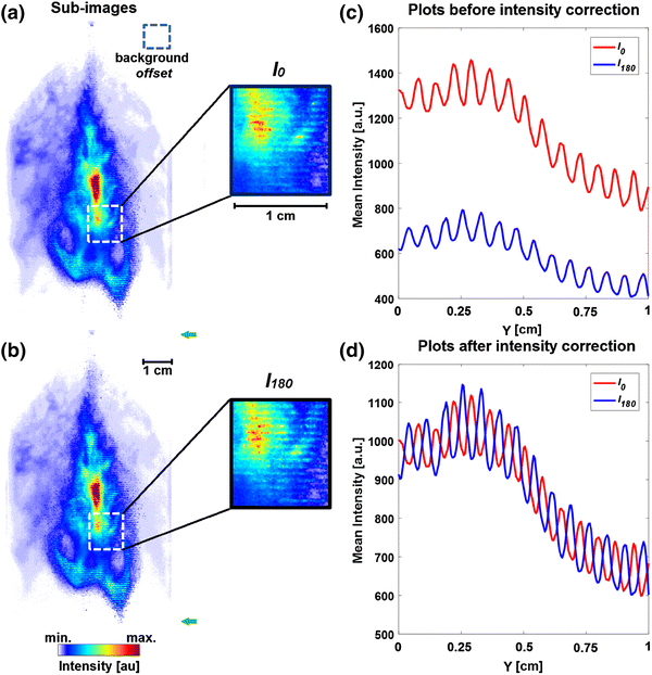
Two modulated LIF sub-images of complementary phase are shown in a and b. The plots of the mean intensity of \(I_{0}\) and \(I_{180}\) from the indicated region (white-dashed box) are given in c without any intensity correction. The same plots are shown in d after the correction procedure for the variations in light intensity
.
- Step 2:
-
The average values of the offset-corrected image, A off, are calculated and the mean value of these M R is deduced. Both offset-corrected sub-images in step 1 are then multiplied by M R and divided by its corresponding A off.
- Step 3:
-
The Fourier transform of both sub-images (from step 2) is calculated and multiplied with a low-pass filter to filter out the modulation. The inverse Fourier transform of these filtered data is then calculated, referred to as I LPF.
- Step 4:
-
The average value of the two I LPF is then calculated, M LPF, and the factor M LPF/ILPF is used as normalization maps for the two sub-images.

Figure 6a, b shows a pair of sub-images (I 0, I 180) recorded with the 2p-SLIPI setup (LIF signal). Figure 6c, d shows plots of the mean intensity of the two images, calculated over the region indicated by the white-dashed boxes in Fig. 6a and b. Figure 6c displays the data before applying any intensity fluctuation corrections, where it can be observed that the detected intensities for the two sub-images are significantly different. Figure 6d shows the outcome of applying steps 1–4, illustrating that such differences can be compensated for computationally. These graphs demonstrate the importance of addressing the issue with intensity variations/fluctuations between the recorded sub-images.
4.3 Subtraction of the sub-images and suppression of residuals
The two sub-images corrected from intensity variations (described in Sect. 4.2) are subtracted and the absolute value of their subtraction \(\left| {I_{0} - I_{180} } \right|\) is deduced. Figure 7a shows one of the modulated sub-images,\(I_{0}\), along with its Fourier transformation. Figure 7b shows \(\left| {I_{0} - I_{180} } \right|\) without applying the intensity correction procedure (see Fig. 6). The image shows an apparent residual line structure, having a spatial frequency corresponding to that of the incident modulation ν as shown by the Fourier transform. Figure 7c is obtained from the absolute value of the subtraction between the two sub-images after applying the correction procedure described in Sect. 4.2. Although less apparent, this image also contains a residual line structure stretching across the entire image. This is also observed in the corresponding Fourier transform, which shows a clear modulation at a spatial frequency twice that of the incident modulation. To obtain a residual-free ‘final’ 2p-SLIPI image, a Gaussian low-pass filter F 2υ is locally applied at the location of the residual frequencies, as shown in Fig. 7d. It should be noted that any structural information appearing periodically at 2ν, i.e., residing within the indicated filter range (see Fig. 7d), is also removed in the final step of the procedure.

Illustration of the post-processing procedure for creating a 2p-SLIPI image from two sub-images. One of the modulated sub-images in a and subtracted images (without the intensity correction) in b along with their Fourier transforms, respectively. c Subtracted image produces an intermediate processed image and its Fourier transform with residuals appearing at 2ν instead of at ν as in b. d ‘Final’ 2p-SLIPI image along with its Fourier transform, where the residuals in c have been suppressed. A band-rejection filter is locally applied in the region indicated in d to remove the residuals
The residuals in Fig. 7c can also be suppressed by a ‘global’ low-pass filter with a cut-off frequency below 2ν. Figure 8 shows a comparison between 2p-SLIPI images constructed using either this approach or the one described in Sect. 4.3. The benefit of the latter approach—locally filter out residual lines—is that it preserves more of the high spatial frequencies, while a possible benefit of the ‘global’ filter approach is that it ensures the data have a uniform spatial frequency response.

2p-SLIPI images, where the residual lines have been suppressed by means of either a local rejection filter in a or a ‘global’ low-pass filter (cutoff below 2ν) in b. In a, parts of the high-frequency image details are lost only in one direction, while preserving in all other directions. In b, the high-frequency image details are lost in all the directions
5 Image post-processing for 1p-SLIPI
5.1 General description
The 1p-SLIPI approach aims at reconstructing the SLIPI image from just one modulated sub-image. It is based on extracting the amplitude of the modulation superimposed on the singly scattered photons. The amplitude can be deduced from the maxima and minima of the modulated signal along each pixel column. This approach, which has been demonstrated both experimentally and with Monte Carlo simulations, is referred to as ‘peak detection’ in this article. Another approach is to use a spatial lock-in algorithm, which has been demonstrated for Rayleigh scattering thermometry of flames (Kempema and Long 2014; Kristensson et al. 2015). In this algorithm, the fundamental frequency (denoted as the “first order” in Fig. 7) of the incident illumination is deduced from the Fourier image. Using this known frequency value, two reference signals (90° phase shifted from each other) are constructed. Then, both vectors are multiplied with each column of the sub-image matrix. Because of this multiplication, in the resulting matrix, all the modulated terms of the column data are demodulated, while the non-modulated “zeroth order” experiences a shift in frequency. As a result, in the Fourier plane, the unwanted frequency components are kept far from the origin while placing the desired frequency of the modulated signal at the center. Applying a Gaussian low-pass filter to this rearranged image matrix permits the retrieval of only the modulated components in the acquired image. The resulting SLIPI image, after the 1p-SLIPI post-processing (see Sects. 5.2, 5.3), losses the original spatial resolution of the recorded sub-image. The spatial resolution is also compromised, because the probed sample cannot be fully illuminated with one-phase structured illumination. Thus, to further improve the spatial resolution of the processed image, it is important to illuminate the sample with as many “line patterns” as possible in a given full field-of-view of the image. Whether the frequency of the incident spatial modulation pattern is high or low can be estimated according to the image full field-of-view offered by the detector chip. For example, in this article, the used “line pattern” of four-line pairs/mm can be considered very high for an image of full field-of-view of 9.7 cm × 8.2 cm. However, it could be too low if the focusing objective is moved towards the light sheet to form a relatively small full field-of-view.
5.2 Approach 1: Detection of the first-order peak
The first-order peak detection approach for generating a 1p-SLIPI image is illustrated in Fig. 9. The modulated sub-image and its FFT are given, in (a, b), respectively. The “first order” and “zeroth order” are indicated in the frequency domain. All frequencies are shifted using the MATLAB function circshift making one of the first orders located now in the center of the Fourier domain as shown in (c). The resulting shifted FFT is called T. The multiplication of T with the desired band-pass filter BPF results in SP, where only the central part of the image is now apparent as shown in (d). The band-pass filter used here is a rotationally symmetric two-dimensional Gaussian low-pass filter. In (e), the desired 1p-SLIPI image is shown, which is obtained by taking the inverse Fourier transform of SP. When comparing the image details between Fig. 9a, e, it can be seen that, in the 1p-SLIPI image, the out-of-focus light effects are suppressed. However, some degradation in image spatial resolution is observable. This degradation is directly related to the dimension of the applied Gaussian low-pass filter, which is itself governed by the fundamental frequency of the incident modulation. Thus, finer incident line structures directly lead to lower losses in image resolution in 1p-SLIPI.

Illustration of the first-order peak detection of 1p-SLIPI post-processing. a, b Modulated sub-image and its FFT, respectively. c Shift of the FFT of the sub-image, where one of the “first order” is now located at the center of the image. d Results of the multiplication between the FFT image in c and a band-pass filter (BPF), for selecting the information represented by the “first order” region only. In e, given the inverse FFT of d, which is the ‘final’ 1p-SLIPI image of the spray
5.3 Approach 2: Lock-in detection algorithm
The lock-in detection algorithm of 1p-SLIPI is illustrated in Fig. 10. The sub-image and its Fourier transform are shown in (a, b), respectively. The first-order peak indicated in (b) corresponds to the modulation frequency of the incident illumination. Using this frequency, two sinusoidal reference signals with a phase difference of 90° are generated as shown in (g) along with their FFT plots. The multiplication between the generated reference signals and the recorded sub-image matrix yields to T1 and T2 as shown in (c). This multiplication allows the “first order” peak and “zeroth order” peak to switch places. Thus, a modulated signal becomes demodulated and vice versa. The signals of interest, SP1 and SP2 shown in (d), are obtained after the multiplication of T1 and T2 with a desired band-pass filter BPF; which is a rotationally symmetric two-dimensional Gaussian low-pass filter. The image (e) is deduced from the square root of the sum of the SP signals in square. Finally, the 1p-SLIPI image shown in (f) is finally deduced from the inverse Fourier transform of the SI signal.

Illustration of the lock-in detection algorithm of 1p-SLIPI. a, and b The modulated sub-image and its FFT, respectively. a The resulting signals T1 and T2 from the multiplication of the sub-image signal and the generated reference signals are shown. The reference signals are generated using the modulated signal frequency (“first order” in FFT), as shown in g. When multiplied with the reference signal, the modulated intensity components of the sub-image in a are demodulated, while the non-modulated components are modulated. d Resulting SP1 and SP2 from the multiplication between the FFT images in c and BPF, respectively. e FFT of the SI signal is calculated. To extract this, first, the inverse FFT of both SP1and SP2 is deduced, and then, the square root of the sum of (SP1)2 and (SP)2 is obtained. f ‘Final’ 1p-SLIPI image of the spray, which is calculated from the inverse FFT of SI signal
To explain the process mathematically, consider a 1D signal, \(I(x)\), which has an amplitude that varies periodically:
where ν equals the spatial frequency given in mm−1 and \(\phi\) is the unknown spatial phase of the modulation. The last term, \(I_{\text{MS}}\), represents the intensity contribution stemming from multiply scattered light, as well as other background light. To remove this undesired contribution and extract the \(I_{\text{S}}\) term, which carries the information from the singly scattered light, the signal is multiplied with two computationally created reference signals, \(R_{1}\) and \(R_{2}\), whose spatial frequencies match the modulation frequency in \(I(x)\), but with a relative phase difference is π/2, according to:
The multiplication between \(I(x)\) and these references yields the following equations:
By analyzing the frequency contents in \(I_{1}\) and \(I_{2}\), one finds that they contain three components: a non-modulated (DC) component and two modulated components, having spatial frequencies of either 2ν or ν. Applying a low-pass filter on these expressions removes the two latter components and thus the \(I_{\text{MS}}\) term, leaving only:
where the tilde assignment indicates the applied low-pass filter. From these two equations, \(\tilde{I}_{\text{S}}\) can finally be calculated:
Here, the desired term \(\tilde{I}_{\text{S}}\) corresponds to the amplitude of the modulation of the modulated signal given in Eq. (5), obtained after operating a low-pass Fourier filtering process.
6 Results comparison between 1p-SLIPI and 2p-SLIPI
6.1 Effects of Fourier filtering on spatial resolution
To analyze the effects of Fourier filtering on image spatial resolution, a sector star target is considered and the resulting images are shown in Fig. 11, where the visibility for each spatial frequency is analyzed. The initial image, the 2p-SLIPI Fourier filtering, and the 1p-SLIPI Fourier filtering images are given in (a–c), respectively. For each of those cases, the low spatial frequencies, which are located at a large distance from the center of the sector star, are clearly visible. However, by zooming in the center of the target, wherethe high frequencies’ information is located, some losses in image resolution are observed, as shown in Fig. 11b, c. For the case of 2p-SLIPI Fourier filtering, this loss in spatial resolution occurs only along the vertical direction and the image details along the horizontal direction are fully preserved. This effect is induced by the local nature of the filtering process used in 2p-SLIPI. For 1p-SLIPI Fourier filtering, the central part of the star target appears blurry with a clear loss in image contrast for all high frequencies’ information. This is due to the Fourier filtering process involved in the 1p-SLIPI process, which smooth out detailed structures of frequencies smaller than the frequency of the incident-modulated illumination.

Effect of Fourier filtering on the image of a sector start target. a Initial image of the target without any Fourier filtering. b, c Fourier filtering applied during 2p-SLIPI and 1p-SLIPI post-processing, respectively. Comparing a with b, loss of image contrast at high frequencies only in the vertical direction while fully preserved in the horizontal of the 2p-SLIPI Fourier filtered image. Comparing c with both a and b, the loss of image contrast is significant at high frequencies in all directions for the 1p-SLIPI Fourier filtering image
6.2 Detection of single and multiple scattering
The numerical modeling of 1p and 2p-SLIPI is performed here by means of Monte Carlo simulation where the modulated light sheet is characterized by a square pattern. The simulated medium is identical than the one presented previously in Sect. 2.2. A modulated light sheet of 532 nm wavelength is crossing a 30 mm side cubic volume containing a distribution of spherical ethanol droplets, as illustrated in Fig. 2. Here, two modulated sub-images with a phase shift of 180° have been generated to reconstruct the 2p-SLIPI image.
The results of the simulation are presented in Fig. 12. It is observed that both the 2p and 1p-SLIPI images show a similar light intensity distribution which is close from the one obtained with the single scattering detection. Similar to the simulated results with 3p-SLIPI given in Sect. 2.2, it is observed that the amount of multiple light scattering intensity suppressed with SLIPI is more than one order of magnitude higher than the desired signal. However, the remaining maximum light intensity detected varies as a function of the filtering process applied. Smoothing effects as well as some edge artifacts are visible on the 1p-SLIPI image due to the employed Fourier filtering post-processing. On the contrary, those effects are not visible on the 2p-SLIPI image.

Results from Monte Carlo simulation for a spatially modulated light sheet (square profile) crossing a homogeneous cubic volume containing ethanol droplets. In a, one modulated sub-image is shown where both the contribution of single and multiple light scattering contribute to the entire detected signal. In b, only the single scattering intensity is given. In c and d, the 2p-SLIPI and 1p-SLIPI images are shown, respectively, demonstrating the possibility in obtaining a signal close to the exact single scattering detection. The graph (e) shows the light intensity integrated along the vertical direction. By closely comparing the exact single scattering intensity with the two SLIPI signals, as shown in f, it is seen that the three curves are close from each other but do not overlap
6.3 Analysis of instantaneous and averaged images of a transient spray
The instantaneous images of LIF and Mie optical signals are shown in Fig. 13 for conventional, 2p-SLIPI, and 1p-SLIPI detections, respectively. The conventional images, referred here as CONV, are deduced by averaging the sub-images, \(I_{0}\) and \(I_{180}\). The LIF images are given in Fig. 13a–c, while the Mie images are given in Fig. 13d–f. It is seen that the conventional LIF and Mie images are affected by the contribution from multiple light scattering. Both the 2p-SLIPI and the 1p-SLIPI methods reject this unwanted signal, thus revealing a more faithful representation of the spray structure within the illumination plane of the light sheet. By comparing the LIF images with the Mie images, the appearance of voids is more pronounced for the LIF signal detection. This can be explained by the fact that the liquid LIF signal generated from the droplets in the spray has a volumetric dependence, whereas the Mie scattering signal is related to the droplet surface area. Thus, the signal difference between small and large droplets is much more pronounced for fluorescence than for Mie scattering. This makes the contribution of small droplet not as visible on the LIF images than for the Mie images. As a result, the larger voids observed on the LIF images contain, in fact, some small droplets which are visible on the Mie images. It is then important to use, when possible, the full dynamic range of the camera on the LIF images. Those effects of signal dependence to the liquid volume and surface lead to a signal intensity distribution which is not similar between the two detections.

Comparison between instantaneous LIF (a–c) and Mie (d–f) images of the DISI sprays for the CONV, 2p-SLIPI, and 1p-SLIPI detections. The conventional images in a, and d suffer from multiple light scattering effects. In contrast, both the 2p-SLIPI and 1p-SLIPI images in b, c and e, f reject this unwanted signal, thus revealing a more faithful representation of the spray within the illumination plane of the light sheet. When comparing SLIPI detections, it is clearly visible that the 1p-SLIPI in c and d appear to have less resolved image detail in comparison to 2p-SLIPI in b and e. When comparing LIF and Mie images, the signal intensity distribution for both is not the same and voids are more pronounced in LIF than in Mie because of droplet volumetric dependence on LIF and surface area dependence on Mie. Such regions can be characterized by the presence of small droplets
From the 2p-SLIPI setup given in Fig. 4, it is important to mention that the linear polarization direction of the first pulse is perpendicular to the linear polarization direction of the second pulse. Thus, the probed droplets should, in this case, remain sufficiently larger than the incident wavelength to obtain an equal level of signal from the two modulated Mie sub-images. In the present conditions, droplets ranging between 5 and 20 µm were illuminated satisfying those conditions. One should rotate the polarization directions by 45° for the cases of Rayleigh scattering detection.
The LIF images averaged over 200 instantaneous images are shown in Fig. 14a–c, for the conventional, 2p-SLIPI, and 1p-SLIPI detections, respectively. Similar to the instantaneous imaging results, the signal from multiple light scattering is evident for the conventional detection. However, in both SLIPI detections, such unwanted signals are removed and the images show a more faithful representation of the spray structures. Interestingly, the differences between the 2p-SLIPI and 1p-SLIPI images are not as important here than for the previously presented results. This can be explained by the fact that image details are smoothed due to averaging removing any sharp gradients and details from instantaneous images. Note that some residual lines can be seen from the zoomed area of the conventional image given in Fig. 14a. Those artifacts are due to the field-dependent intensity fluctuation in between the two modulated sub-images, as shown in Fig. 4d. In some situations, \(I_{180}\) has a higher amplitude of the modulation than for \(I_{0}\), despite the correction for light intensity fluctuations. Therefore, some residual lines can, in such cases, still remain on the final processed images.
A summary of all pros and cons of the two techniques, which has been demonstrated in this article, is given in Table 1. The requirements regarding the respective optical setups are also included.

Averaged LIF images of the DISI spray, over 200 instantaneous images. The conventional, 2p-SLIPI, and 1p-SLIPI detections are given in a–c, respectively. In a, the conventional image suffers from multiple light scattering effects. The 2p-SLIPI in b and 1p-SLIPI in c efficiently remove the unwanted signal intensity and provide a more reliable representation of spray structures. Note that in this case of averaged imaging, the two SLIPI methods give more similar images than for instantaneous imaging
7 Conclusions
In conclusion, both 1p and 2p SLIPI techniques are capable of suppressing most of the unwanted effects caused by the detection of multiple light scattering, rendering large improvements in image contrast when applied for spray visualization. Both techniques are suitable for instantaneous imaging for the studies of spray dynamics and fast liquid/air mixing, where the undesired surrounding light induced by the incident illumination needs to be suppressed. However, while similar global spray features are obtained, there is a clear difference between the two approaches concerning spatial resolution. The 2p-SLIPI preserves nearly the full spatial resolution offered by the imaging system, rejecting only some specific high spatial frequencies (those coinciding with residual structures). On the contrary, a 1p-SLIPI system provides images with less clarity as it rejects all high spatial frequencies above the frequency of the incident illumination. Depending on the applied modulation frequency, certain fine structural details in the spray may, therefore, be unresolvable with a 1p-SLIPI setup.
In terms of the optical arrangement, the 2p-SLIPI approach is more complex, since it requires the use of two pulsed laser systems and a detector capable of recording the two sub-images on a sub-microseconds time scale to freeze the motion of the spray. In addition, the thickness of the calcite crystal needs to perfectly agree with the modulation frequency and the wavelength used, so that the phase shift induces equals half the modulation period. The optical design of 1p-SLIPI is significantly less complicated and less demanding in terms of optical arrangement/alignment and of hardware requirements. Thus, 1p-SLIPI can easily be combined with other existing planar-based imaging techniques.
Finally, as the level of details provided by the two methods differs, this will determine which of the two techniques fits best to a given application. If only the global spray structures are sought, the less complicated 1p-SLIPI setup will suffice. However, if the detailed study of the droplet cloud is desired, the 2p-SLIPI would be more suitable.
References
Adrian RJ, Westerweel J (2011) Particle image velocimetry. Cambridge University Press, Cambridge
Bachalo WD, Houser MJ (1984) Phase/Doppler spray analyzer for simultaneous measurements of drop size and velocity distributions. OPTICE 23:235583. doi:10.1117/12.7973341
Berrocal E (2006) Multiple scattering of light in optical diagnostics of dense sprays and other complex turbid media. Ph. D. Thesis, Cranfield University, Cranfield
Berrocal E, Kristensson E, Richter M, Linne MA, Aldén M (2008) Application of structured illumination for multiple scattering suppression in planar laser imaging of dense sprays. Opt Express 16:17870–17881. doi:10.1364/OE.16.017870
Berrocal E, Kristensson E, Sedarsky DML (2009) Analysis of the SLIPI technique for multiple scattering suppression in planar imaging of fuel sprays ICLASS 2009. In: 11th triennial international annual conference on liquid atomization and spray systems, Vail, Colorado USA
Berrocal E, Johnsson J, Kristensson E, Alden M (2012) Single scattering detection in turbid media using single-phase structured illumination filtering. J Eur Opt Soc Rapid Publ 7
Brübach J, Patt A, Dreizler A (2006) Spray thermometry using thermographic phosphors. Appl Phys B 83:499. doi:10.1007/s00340-006-2244-8
Bruchhausen M, Guillard F, Lemoine F (2005) Instantaneous measurement of two-dimensional temperature distributions by means of two-color planar laser induced fluorescence (PLIF). Exp Fluids 38:123–131. doi:10.1007/s00348-004-0911-2
Charalampous G, Hardalupas Y, Taylor AMKP (2009) Novel technique for measurements of continuous liquid jet core in an atomizer. AIAA J 47:2605–2615. doi:10.2514/1.40038
Cole MJ, Siegel J, Webb SED et al (2001) Time-domain whole-field fluorescence lifetime imaging with optical sectioning. J Microsc 203:246–257. doi:10.1046/j.1365-2818.2001.00894.x
Crua C, Heikal MR, Gold MR (2015) Microscopic imaging of the initial stage of diesel spray formation. Fuel 157:140–150. doi:10.1016/j.fuel.2015.04.041
Dodge LG, Rhodes DJ, Reitz RD (1987) Drop-size measurement techniques for sprays: comparison of Malvern laser-diffraction and Aerometrics phase/Doppler. Appl Opt 26:2144–2154. doi:10.1364/AO.26.002144
Domann R, Hardalupas Y (2003) Quantitative measurement of planar droplet Sauter mean diameter in sprays using planar droplet sizing. Part Part Syst Charact 20:209–218. doi:10.1002/ppsc.200390027
Fansler T, Parrish S (2015) Spray measurement technology: a review. Meas Sci Technol 26:012002
Halls BR, Heindel TJ, Kastengren AL, Meyer TR (2014) Evaluation of X-ray sources for quantitative two- and three-dimensional imaging of liquid mass distribution in atomizing sprays. Int J Multiph Flow 59:113–120. doi:10.1016/j.ijmultiphaseflow.2013.10.017
Kempema NJ, Long MB (2014) Quantitative Rayleigh thermometry for high background scattering applications with structured laser illumination planar imaging. Appl Opt 53:6688–6697. doi:10.1364/AO.53.006688
Kristensson E (2012) Structured laser illumination planar imaging SLIPI applications for spray diagnostics. PhD Thesis, Lund University, Lund
Kristensson E, Berrocal E, Richter M, Aldén M (2010) Nanosecond structured laser illumination planar imaging for single-shot imaging of dense sprays. Atom Sprays 20:337–343. doi:10.1615/AtomizSpr.v20.i4.50
Kristensson E, Araneo L, Berrocal E et al (2011) Analysis of multiple scattering suppression using structured laser illumination planar imaging in scattering and fluorescing media. Opt Express 19:13647–13663. doi:10.1364/OE.19.013647
Kristensson E, Berrocal E, Aldén M (2014) Two-pulse structured illumination imaging. Opt Lett 39:2584–2587. doi:10.1364/OL.39.002584
Kristensson E, Ehn A, Bood J, Aldén M (2015) Advancements in Rayleigh scattering thermometry by means of structured illumination. Proc Combust Inst 35:3689–3696. doi:10.1016/j.proci.2014.06.056
Le Gal P, Farrugia N, Greenhalgh DA (1999) Laser sheet dropsizing of dense sprays. Opt Laser Technol 31:75–83. doi:10.1016/S0030-3992(99)00024-9
Lee K, Abraham J (2011) Spray applications in internal combustion engines. In: Ashgriz N (ed) Handbook of atomization and sprays: theory and applications. Springer, US, pp 777–810
Linne MA (2013) Imaging in the optically dense regions of a spray: a review of developing techniques. Prog Energy Combust Sci 39:403–440. doi:10.1016/j.pecs.2013.06.001
Linne MA, Paciaroni M, Berrocal E, Sedarsky D (2009) Ballistic imaging of liquid breakup processes in dense sprays. Proc Combust Inst 32:2147–2161. doi:10.1016/j.proci.2008.07.040
Mishra YN, Kristensson E, Berrocal E (2014) Reliable LIF/Mie droplet sizing in sprays using structured laser illumination planar imaging. Opt Express 22:4480–4492. doi:10.1364/OE.22.004480
Mishra YN, Abou Nada F, Polster S, Kristensson E, Berrocal E (2016) Thermometry in aqueous solutions and sprays using two-color LIF and structured illumination. Opt Express 24:4949–4963. doi:10.1364/OE.24.004949
Neil MAA, Juškaitis R, Wilson T (1997) Method of obtaining optical sectioning by using structured light in a conventional microscope. Opt Lett 22:1905–1907. doi:10.1364/OL.22.001905
Omrane A, Särner G, Aldén M (2004) 2D-temperature imaging of single droplets and sprays using thermographic phosphors. Appl Phys B 79:431–434. doi:10.1007/s00340-004-1584-5
Storch, Mishra, Koegl, Kristensson, Will, Zigan, Berrocal (2016) Two-phase SLIPI for instantaneous LIF and Mie imaging of transient fuel sprays. Opt Lett 41:5422–5425. doi:10.1364/OL.41.005422
Vetrano MR, Simonini A, Steelant J, Rambaud P (2013) Thermal characterization of a flashing jet by planar laser-induced fluorescence. Exp Fluids 54:1573. doi:10.1007/s00348-013-1573-8
Wellander R, Berrocal E, Kristensson E, Richter M, Aldén M (2011) Three-dimensional measurement of the local extinction coefficient in a dense spray. Meas Sci Technol 22:125303
Westerweel J, Elsinga GE, Adrian RJ (2013) Particle image velocimetry for complex and turbulent flows. Annu Rev Fluid Mech 45:409–436. doi:10.1146/annurev-fluid-120710-101204
Acknowledgements
This project has received funding from the European Research Council (ERC) under the European Union’s Horizon 2020 research and innovation programme (Agreement No. 638546—ERC starting Grant “Spray Imaging”). The funding support from the Erlangen Graduate School in Advanced Optical Technologies (SAOT) is also greatly acknowledged.
Author information
Authors and Affiliations
Corresponding author
Rights and permissions
Open Access This article is distributed under the terms of the Creative Commons Attribution 4.0 International License (http://creativecommons.org/licenses/by/4.0/), which permits unrestricted use, distribution, and reproduction in any medium, provided you give appropriate credit to the original author(s) and the source, provide a link to the Creative Commons license, and indicate if changes were made.
About this article

Cite this article
Mishra, Y.N., Kristensson, E., Koegl, M. et al. Comparison between two-phase and one-phase SLIPI for instantaneous imaging of transient sprays. Exp Fluids 58, 110 (2017). https://doi.org/10.1007/s00348-017-2396-9
Received:
Revised:
Accepted:
Published:
DOI: https://doi.org/10.1007/s00348-017-2396-9