Unitary Anchored Planar Algebras

Abstract

In our previous article (http://arxiv.org/abs/1607.06041), we established an equivalence between pointed pivotal module tensor categories and anchored planar algebras. This article introduces the notion of unitarity for both module tensor categories and anchored planar algebras, and establishes the unitary analog of the above equivalence. Our constructions use Baez’s 2-Hilbert spaces (i.e., semisimple $\textrm{C}^*$-categories equipped with unitary traces), the unitary Yoneda embedding, and the notion of unitary adjunction for dagger functors between 2-Hilbert spaces.

1 Introduction

Planar algebras were introduced by Vaughan Jones in [Jon21]. A planar algebra $\mathcal {P}$ is a collection of vector spaces $\mathcal {P}[n]$, called box-spaces, indexed by the nonnegative integers, along with a linear map

$$\begin{aligned} Z(T): \mathcal {P}[n_1]\otimes \cdots \otimes \mathcal {P}[n_k]\longrightarrow \mathcal {P}[n_0] \end{aligned}$$

for every planar tangle T. These maps are required to be compatible with the operation of composition of tangles in the sense that $Z(S\circ _i T) = Z(S)\circ ({{\,\textrm{id}\,}}\otimes \ldots \otimes {{\,\textrm{id}\,}}\otimes Z(T)\otimes {{\,\textrm{id}\,}}\otimes \ldots \otimes {{\,\textrm{id}\,}})$. See Sect. 4.1 for more details.

In [HPT23b], we internalised the notion of planar algebra to the context of a pivotal braided tensor category $\mathcal {V}$, and called the resulting notion an anchored planar algebra. The box-spaces $\mathcal {P}[n]$ of an anchored planar algebra are now objects of our ambient category $\mathcal {V}$, and we have morphisms

$$\begin{aligned} Z(T): \mathcal {P}[n_1]\otimes \cdots \otimes \mathcal {P}[n_k]\longrightarrow \mathcal {P}[n_0] \end{aligned}$$

for every anchored planar tangle. For example:

The full definition is given in §4.2.

We then proceeded to establish an equivalence of categories

$$\begin{aligned} \left\{ \begin{array}{l} \mathrm{Anchored\, planar\, algebras\, in\, } \mathcal {V}\\ \end{array} \right\} \,\,\,\,\cong \,\, \left\{ \begin{array}{l} \mathrm{Pointed\, pivotal\, module\,} \\ \mathrm{tensor\, categories\, over\,} \mathcal {V}\end{array} \right\} \end{aligned}$$

between the category $\textsf{APA}$ of anchored planar algebras in $\mathcal {V}$, and the category $\textsf{ModTens}_*$ of pointed¹ pivotal module tensor categories over $\mathcal {V}$ whose action functor admits a right adjoint. We refer the reader to §3.1 below for definitions of these notions.

In this paper we further specialise/generalise the notion of anchored planar algebra to the context when $\mathcal {V}$ is a unitary pivotal braided tensor category, and we prove an analog of the above result. This is motivated by enriched subfactor theory [JL17], bicommutant categories [Hen17b, HP17, HP23], topological orders [HBJP23], and higher unitary categories [CHPJP22, DHP22].

Let $\mathcal {V}$ be a braided unitary tensor category equipped with a unitary dual functor (the latter is the unitary analog of a pivotal structure [Yam04, Sel11, Pen20]; see §2.2 below for more details). A unitary module tensor category $\mathcal {C}$ is called pivotal if it is equipped with a unitary dual functor, compatibly with the action of $\mathcal {V}$. Our main result is the unitary analog of Theorem [HPT23b, Thm. A]:

Theorem A

There is an equivalence of categories²

$$\begin{aligned} \left\{ \begin{array}{l} \mathrm{Unitary\, anchored\, planar\, algebras\, in\, } \mathcal {V}\end{array} \right\} \cong \left\{ \begin{array}{l} \mathrm{Unitary\, pointed\, pivotal\, module\, tensor\, }{}^{3} \\ \mathrm{categories\, over} \mathcal {V}, \mathrm{with\, chosen\, state}. \end{array} \right\} \end{aligned}$$

Moreover,³ when $\mathcal {V}$ is ribbon, spherical unitary anchored planar algebras correspond under this equivalence to unitary module tensor categories whose chosen state is spherical.

1.1 Motivations for this article

1.1.1 Enriched subfactor theory

The development of planar algebras [Jon21] is intimately linked to subfactor theory. We expect a similar relation to hold between anchored planar algebras and enriched subfactor theory. In their paper [JP17], Corey Jones and the second author introduced a notion of $\textrm{W}^*$-algebra object A internal to a unitary tensor category $\mathcal {V}$. One could imagine formulating an analog of the notion of $\textrm{II}_{1}$ factor internal to $\mathcal {V}$ (perhaps just the condition that the neutral part of A, i.e. $\mathcal {V}(1\rightarrow A)$, is a $\textrm{II}_1$ factor) and, similarly, a notion of subfactor internal to $\mathcal {V}$.

We conjecture that, in this context, the correct analog of the standard invariant is that of a unitary anchored planar algebra:

Conjecture 1.1

The enriched standard invariant of a subfactor internal to $\mathcal {V}$ is a 2-shaded unitary anchored planar algebra in $Z(\mathcal {V})$. Finite index, finite depth hyperfinite $\textrm{II}_1$ subfactors internal to $\mathcal {V}$ are classified by their enriched standard invariants⁴.

As an example, in [JL17, Rem. 6.1], Jaffe and Liu construct a subfactor from the inductive limit of parafermion algebras, and obtain the parafermion subfactor planar para algebra from its ‘graded standard invariant.’ Planar para algebras are anchored planar algebras internal to $\mathcal {V}=\textsf{Vect}(\mathbb {Z}/N)$ with a particular braiding (see [HPT23b, Examples 3.7 and 3.8]), and the parafermion planar para algebra corresponds to a Tambara-Yamagami module tensor category over $\mathcal {V}$.

There is a classification of $\textrm{II}_1$ subfactors with index less than 4 [Jon83, GdlHJ89, Kaw95, BN91, Izu94] in terms of ADE Coxeter-Dynkin diagrams (where $D_{\text {odd}}$ and $E_{7}$ do not occur, and $E_6$ and $E_8$ occur twice). For subfactors enriched over super vector spaces, the non-simply laced Coxeter-Dynkin diagrams $C_{\text {even}}$ and $F_4$ also appear [ALW19, §6-7].

1.1.2 Internal structure of bicommutant categories

Bicommutant categories were introduced in [Hen17b], as higher categorical analogs of von Neumann algebras. The simplest example of a bicommutant category is $\textsf{Bim}(M)$, the tensor category of all bimodules over a von Neumann algebra M. Examples corresponding to unitary fusion categories were constructed in [HP17], and further studied in [HP23]. Examples corresponding to conformal nets were constructed in [Hen17a].

When $M=R$ is a hyperfinite $\textrm{II}_1$, $\textrm{II}_\infty$, or $\textrm{III}_1$ factor, there is a well-known correspondence [Pop90, Pop95, Jon21, Tom21, BCE+20] between conjugacy classes of finite depth R-R bimodules and isomorphism classes of unitary finite depth planar algebras⁵:

$$\begin{aligned} \left\{ \begin{array}{l} \text {Finite depth} R-R-\text {bimodules} \end{array} \right\} \bigg / \text {conj.} \,\leftrightarrow \left\{ \begin{array}{l} \text {Connected finite depth} \\ \text {unitary planar algebras} \end{array} \right\} \bigg / \text {iso.} \end{aligned}$$

We conjecture that, under suitable assumptions, conjugacy clases of finite depth objects in a bicommutant category $\mathcal {T}$ are in bijective correspondence with finite depth unitary anchored planar algebras in $Z(\mathcal {T})$.

Conjecture 1.2

Let $\mathcal {T}$ be a bicommutant category whose Drinfeld center $Z(\mathcal {T})$ is fusion. Then, under suitable assumptions, there exists a natural bijective correspondence

$$\begin{aligned} \left\{ \begin{array}{l} \textrm{Finite depth objects of} \mathcal {T}\end{array} \right\} \bigg / \text { conj.} \,\leftrightarrow \left\{ \begin{array}{l} \textrm{Connected finite depth unitary} \\ \textrm{anchored planar algebras in} \mathcal {Z}(\mathcal {T}) \end{array} \right\} \bigg / \text {iso.} \end{aligned}$$

For bicommutant categories coming from fusion categories, Conjecture 1.2 was proven in our recent paper [HPT23a].

1.1.3 (2+1)D topological orders

Topological order is a phenomenon in (theoretical) condensed matter physics beyond Landau’s symmetry breaking paradigm. In (2+1) dimensions, the low energy effective field theory of a topologically ordered phase of matter is a topological quantum field theory, and the low energy localised excitations form a unitary modular tensor category (UMTC).

Conjecture 1.3

Let $\mathcal {X}$ and $\mathcal {Y}$ be $(2+1)$D topological orders with the same anomaly, let $\mathcal {M}$ be a topological domain wall between them, and let m be a symmetrically self-dual point-like excitation that lives on $\mathcal {M}$. Then the collection of objects

(where the red dots represent m) in the unitary modular tensor category associated to $\mathcal {X}$ are the box-spaces of a unitary anchored planar algebra.

More generally, if $\mathcal {U}$ is any unitary 3-category (a notion yet to be defined) and $c:v\rightarrow w$ is a dualizable 1-morphism between dualizable objects, then $\mathcal {V}:={{\,\textrm{End}\,}}(1_{v})$ should be a unitary modular ribbon category and $\mathcal {C}:={{\,\textrm{End}\,}}(c)$ should be a unitary $\mathcal {V}$-module multifusion category. Moreover, for $m:c\Rightarrow c$ symmetrically self-dual, the objects ${\underline{{{\,\textrm{Hom}\,}}}}(1_c, m^{\otimes k})\in \mathcal {V}$ should form the box-spaces of a unitary anchored planar algebra.

Indeed, it should be the case that (2+1)D topological orders with the a given anomaly form a unitary 3-category whose 1-morphisms are topological domain walls and whose higher morphisms correspond to topological defects of higher codimension. More precisely, [HBJP23] posits that for a UMTC $\mathcal {A}$ whose Witt class represents an anomaly, the 3-category of $\mathcal {A}$-enriched unitary fusion categories describes this putative 3-category of (2+1)D topological orders.

1.1.4 Unitary higher categories

Over the past decades, a theory of higher linear algebra has emerged from work of many authors, e.g., [BD95, Bae97, Lur09, HV19]. The higher n-category $n\textsf{Vect}$ of n-vector spaces may be used as target for n-dimensional topological quantum field theories, where the fully dualizable objects give fully extended theories by the corbordism hypothesis. Until recently, definitions of $n\textsf{Vect}$ were bespoke, chosen to agree with well-known state-sum models. The recent breakthrough [GJF19] provides a uniform framework to construct (the fully dualizable part of) $n\textsf{Vect}$ via a formal inductive procedure starting from just the complex numbers.

Starting with $\mathbb {C}$, a commutative algebra, we can deloop and complete to obtain the 1-category $\mathsf {Vect_{fd}}$. Since $\textsf{Vect}$ is a symmetric monoidal tensor category, we can deloop and complete again to obtain the 2-category $\mathsf {Alg_{fd}^{sep}}$ of finite dimensional separable algebras, bimodules, and intertwiners. Assigning to an algebra its category of modules gives an equivalence to $2\textsf{Vect}$, the 2-category of finite semisimple categories, linear functors, and natural transformations. Since $2\textsf{Vect}$ is a symmetric monoidal 2-category, we may deloop and complete again to obtain the 3-category of (separable) multifusion categories [JF22], which is equivalent to the 3-category of semisimple 2-categories [DR18, Déc22].

$$\begin{aligned} \mathbb {C}\xrightarrow {\Sigma } \mathsf {Vect_{fd}} \xrightarrow {\Sigma } \mathsf {Alg_{fd}^{sep}} \simeq \mathsf {LinCat_{fin}^{ss}} \xrightarrow [28]{\Sigma } \textsf{MultFusCat} \underset{[9]}{\simeq } \mathsf {Lin2Cat_{fin}^{ss}} \xrightarrow {\Sigma } \cdots \end{aligned}$$

(1)

For physical applications in topologically ordered phases of matter, it is important to have a version of the above construction that incorporates unitary structures at all levels. However, extending this construction to the unitary setting is quite delicate. Whereas dualizability is a property in the non-unitary setting, it is additional structure in the unitary setting [Yam04, Pen20]. Thus $n\textsf{Hilb}$ should come with canonical involutions corresponding to duals at various levels.

Writing this article has allowed us to clarify these notions for $2\textsf{Hilb}$. Here, a 2-Hilbert space [Bae97] is a linear category (enriched in finite dimensional vector spaces) equipped with Hilbert space structures on hom spaces satisfying

$$\begin{aligned} \langle f , h \circ g^\dag \rangle _{b\rightarrow c} \!=\!\langle f\circ g , h \rangle _{a\rightarrow c} \!=\!\langle g , f^\dag \circ h \rangle _{a\rightarrow b} \quad \forall \, g:a\rightarrow b,\, f:b\!\rightarrow \! c,\, h: a\!\rightarrow \! c. \end{aligned}$$

As pointed out in [GMP+23, Rem. 3.6.1], 2-Hilbert spaces are the natural setting for defining the unitary Yoneda embedding [JP20]. In turn, we have a well-behaved notion of unitary adjunction for dagger functors, which we describe in §2.1 below. In Proposition 2.8 (see also Remark 2.9) we prove that unitary adjunction gives a canonical unitary dual functor on $2\textsf{Hilb}$. We expect this to be a key ingredient in defining higher dagger idempotents, for the unitary analog of (1).

1.2 Outline

In §2, we provide the preliminary background for this article, together with some new contributions for unitary and involutive categories. We discuss the unitary Yoneda embedding and unitary adjunction in §2.1, and we review unitary dual functors and spherical states in §2.2. In §2.3, we use the graphical calculus for the 2-category $\textsf{Cat}$ to transport involutive structures through adjunctions.

In §3, we review the notion of pivotal module tensor category over a braided pivotal category before introducing the unitary counterpart in §3.2. We briefly review the graphical calculus of strings on tubes for the categorified trace from [HPT16], and we study the adjoint of the unit map in §3.3. In the spherical setting, we prove unitarity of the traciator in §3.4.

In §4, we review the notions of planar algebra and anchored planar algebra before introducing the unitary counterparts in §4.3. We show that for a spherical unitary anchored planar algebra, the adjoint is compatible with the inside-out reflection of tangles in Proposition 4.8. Finally, in §5, we prove our main Theorem A.

2 Preliminaries

Our standard references for (unitary) tensor categories include [LR97, GLR85, Sel11, EGNO15, HPT16, Pen20].

Let $\textsf{Cat}_\mathbb {C}$ be the 2-category of $\mathbb {C}$-linear categories, linear and anti-linear functors, and natural transformations. We only allow natural transformations between functors if they are either both linear or both anti-linear. In this section, we shall often use the graphical calculus for $\textsf{Cat}_\mathbb {C}$, denoting linear categories by two-dimensional regions, functors by strands, and natural transformations by junctures. As in [CP22], we may identify a category $\mathcal {A}$ with the category of $\mathbb {C}$-linear functors $\textsf{Vect}\rightarrow \mathcal {A}$. Given a functor $F: \mathcal {A}\rightarrow \mathcal {B}$ and objects $a\in \mathcal {A}$ and $b\in \mathcal {B}$, this allows us to give a graphical representation e.g. for a morphism $f:F(a)\rightarrow b$, as follows:

Given an adjunction $F\dashv G$ between two functors $F: \mathcal {A}\rightarrow \mathcal {B}$ and $G: \mathcal {B}\rightarrow \mathcal {A}$, recall that $f: F(a) \rightarrow b$ and $g:A\rightarrow G(b)$ are called mates if they are mapped to one another under the natural isomorphism

$$\begin{aligned} \mathcal {B}\big (F(a) \rightarrow b\big )&\,\,\cong \,\, \mathcal {A}\big (a \rightarrow G(b)\big )\\ f \qquad&\,\,\leftrightarrow \,\,\,\,\,\,\, {{\,\textrm{mate}\,}}(f)\\ {{\,\textrm{mate}\,}}(g) \,\,\,\,&\,\,\leftrightarrow \,\,\qquad g. \end{aligned}$$

Mates are represented in the graphical calculus as follows:

where the cup and cap represent the unit and counit of the adjunction.

The operations of taking the mate are natural with respect to pre-composition and post-composition by another morphism:

• (M1) ${{\,\textrm{mate}\,}}(f_2\circ f_1) = G(f_2) \circ {{\,\textrm{mate}\,}}(f_1)$ for all $f_1:F(a)\rightarrow b_1$ and $f_2: b_1\rightarrow b_2$.

• (M2) ${{\,\textrm{mate}\,}}(g_2\circ g_1) = {{\,\textrm{mate}\,}}(g_2) \circ F(g_1)$ for all $g_1: a_1\rightarrow a_2$ and $g_2:a_2\rightarrow G(b)$.

2.1 The unitary Yoneda lemma and unitary adjunctions

In this section, we work with semisimple $\textrm{C}^{*}$ categories. (Note that every Cauchy complete $\textrm{C}^{*}$ category with finite dimensional hom spaces is semisimple [GMP+23, §3.1.1].)

Definition 2.1

A unitary trace on a semisimple $\textrm{C}^{*}$ category $\mathcal {A}$ is a collection of linear maps ${{\,\textrm{Tr}\,}}_a: \mathcal {A}(a\rightarrow a) \rightarrow \mathbb {C}$, for all $a\in \mathcal {A}$, satisfying

• ${{\,\textrm{Tr}\,}}_a(f\circ g)= {{\,\textrm{Tr}\,}}_b(g\circ f)$ for all $f: a\rightarrow b$ and $g: b\rightarrow a$, and

• The sesquilinear forms $\langle f, g\rangle _{a\rightarrow b}:={{\,\textrm{Tr}\,}}_a(g^\dag \circ f)$ are positive definite.

The above inner products satisfy

$$\begin{aligned} \langle f , h \circ g^\dag \rangle _{b\rightarrow c} =\langle f\circ g , h \rangle _{a\rightarrow c} =\langle g , f^\dag \circ h \rangle _{a\rightarrow b} \quad \forall \, g:a\rightarrow b,\, f:b\rightarrow c,\, h: a\rightarrow c,\nonumber \\ \end{aligned}$$

(2)

equivalently

$$\begin{aligned} (-\circ g)^\dagger =-\circ g^\dagger \qquad \text {and}\qquad (f\circ -)^\dagger =f^\dagger \circ -, \end{aligned}$$

(3)

and thus equip $\mathcal {A}$ with the structure of a 2-Hilbert space in the sense of [Bae97]. Conversely, one may recover the trace from the 2-Hilbert space structure by the formula ${{\,\textrm{Tr}\,}}_a(f):=\langle f, {{\,\textrm{id}\,}}_a\rangle _{a\rightarrow a}$. The notion of semisimple $\textrm{C}^{*}$ category equipped with a unitary trace is thus equivalent to the notion of 2-Hilbert space.

The first condition in (3) implies that for all $c\in \mathcal {A}$, the functor $\mathcal {A}(-\rightarrow c): \mathcal {A}^{{{\,\textrm{op}\,}}} \rightarrow \textsf{Hilb}$ is a $\dagger$-functor, and the second equality implies that the unitary Yoneda embedding

$$\begin{aligned} \mathcal {A}\,\,\,\hookrightarrow \,\,\, \textsf{Fun}^\dag (\mathcal {A}^{{{\,\textrm{op}\,}}}\rightarrow \textsf{Hilb}) \end{aligned}$$

(4)

is a $\dagger$-functor (where $\textsf{Fun}^\dag (\mathcal {A}^{{{\,\textrm{op}\,}}}\rightarrow \textsf{Hilb})$ denotes the $\dagger$-category of $\dagger$-functors $\mathcal {A}^{{{\,\textrm{op}\,}}}\rightarrow \textsf{Hilb}$).

The above facts were first observed in [GMP+23, Rem. 3.61 and footnote], and we shall refer to them collectively as the unitary Yoneda lemma. Note that the essential image of (4) is the same as its unitary essential image (using polar decomposition in $\textsf{Fun}^\dag (\mathcal {A}^{{{\,\textrm{op}\,}}}\rightarrow \textsf{Hilb})$), so a $\dagger$-functor $\mathcal {A}^{{{\,\textrm{op}\,}}} \rightarrow \textsf{Hilb}$ is unitarily representable if and only if the underlying functor is representable. Given a $\dagger$-functor $F\in \textsf{Fun}^\dag (\mathcal {A}^{\textrm{op}}\rightarrow \textsf{Hilb})$ in the essential image of (4), a representing object is given by

$$\begin{aligned} c := \bigoplus _{a\in {{\,\textrm{Irr}\,}}(\mathcal {A})} d_a^{-1}F(a)\otimes a, \end{aligned}$$

(5)

where $d_a:={{\,\textrm{Tr}\,}}^\mathcal {A}_a({{\,\textrm{id}\,}}_a)$, ${{\,\textrm{Irr}\,}}(\mathcal {A})$ is a basis⁶ of $\mathcal {A}$, and we use the notation $\lambda H$ to denote the Hilbert space with the same underlying vector space as H and inner product $\lambda \langle \,\cdot \,,\,\cdot \,\rangle _H$. The rescaling of the inner product of F(a) ensures the unitarity of the isomorphism $\mathcal {A}(-\rightarrow c)\cong F$ given by

$$\begin{aligned} \mathcal {A}\left( b\rightarrow \bigoplus _{a\in {{\,\textrm{Irr}\,}}(\mathcal {A})} d_a^{-1}F(a)\otimes a\right) \cong d_b^{-1}F(b)\otimes \mathcal {A}(b\rightarrow b) \xrightarrow {{{\,\textrm{id}\,}}_{F(b)}\otimes ({{\,\textrm{id}\,}}_b\mapsto 1)} F(b) \end{aligned}$$

(6)

for $b\in {{\,\textrm{Irr}\,}}(\mathcal {A})$.

Remark 2.2

If $\mathcal {A}$ is finitely semisimple and $\textsf{Hilb}$ is taken to mean finite dimensional Hilbert spaces, then (4) is a $\dag$-equivalence.

Definition 2.3

Let $(\mathcal {A},{{\,\textrm{Tr}\,}}^\mathcal {A})$ and $(\mathcal {B},{{\,\textrm{Tr}\,}}^\mathcal {B})$ be semisimple $\textrm{C}^{*}$ categories equipped with unitary traces. A unitary adjunction, denoted $F\dashv ^\dag G$, consists of linear $\dagger$-functors $F: \mathcal {A}\rightarrow \mathcal {B}$ and $G: \mathcal {B}\rightarrow \mathcal {A}$ and a family of unitary and natural isomorphisms

$$\begin{aligned} \psi _{a,b}:\mathcal {B}(F(a) \rightarrow b) \xrightarrow {\,\,\cong \,\,} \mathcal {A}(a\rightarrow G(b)). \end{aligned}$$

(7)

If F and G are instead antilinear $\dagger$-functors, and (7) is antiunitary, then adjunction is called an antiunitary adjunction.

Remark 2.4

In the above definition, if we had merely required F and G to be (anti)linear functors, they would nevertheless automatically be $\dagger$-functors. We prove that G is a dagger functor (the argument for F is similar). For any $f \in \mathcal {B}(b_1\rightarrow b_2)$, the following diagram commutes:

Applying $\dagger$ to all the arrows, by (3), the following diagram also commutes:

As $G(f^\dagger )\circ -$ also makes that second diagram commute, $G(f^\dagger )\circ - = G(f)^\dagger \circ -$, and hence $G(f^\dag )=G(f)^\dag$.

Similarly, whenever $F\dashv G$ are adjoint functors between linear categories, if (7) is (anti)linear, then F and G are automatically (anti)linear functors.

The above facts are reminiscent of the well-known fact that if H, K are Hilbert spaces and $S: H \rightarrow K$ and $T: K\rightarrow H$ are two functions such that $\langle S\eta , \xi \rangle = \langle \eta , T\xi \rangle$ for all $\eta \in H$ and $\xi \in K$, then S and T are automatically bounded linear maps.

Lemma 2.5

Let $(\mathcal {A},{{\,\textrm{Tr}\,}}^\mathcal {A})$ and $(\mathcal {B},{{\,\textrm{Tr}\,}}^\mathcal {B})$ be semisimple $\textrm{C}^{*}$ categories with unitary traces, and let $F: \mathcal {A}\rightarrow \mathcal {B}$ be a linear $\dagger$-functor that has a right adjoint. Then F also has a unitary right adjoint. The unitary right adjoint G is unique up to unique unitary natural isomorphism, and given by

$$\begin{aligned} G(b)\,= \bigoplus _{a\in {{\,\textrm{Irr}\,}}(\mathcal {A})} d_a^{-1}\mathcal {B}\big (F(a)\rightarrow b\big ) \otimes a. \end{aligned}$$

(8)

The same holds true for antilinear $\dagger$-functors.

Proof

The unitary right adjoint G, if it exists, sends $b\in \mathcal {B}$ to the object representing the $\dagger$-functor

$$\begin{aligned} a\mapsto \mathcal {B}\big (F(a)\rightarrow b\big ). \end{aligned}$$

(9)

By the unitary Yoneda Lemma, such a representing object, if it exists, is unique up to unique unitary isomorphism. We get (8) by substituting (9) into (5). If F admits a right adjoint, the functors (9) are representable, hence unitarily representable, hence F admits a unitary right adjoint.

Finally, antilinear $\dagger$-functors are the same thing as linear $\dagger$-functors $\mathcal {A}\rightarrow {\overline{\mathcal {B}}}$, so the same results hold true for antilinear $\dagger$-functors. $\square$

Lemma 2.6

If ${{\,\textrm{coev}\,}}$ and ${{\,\textrm{ev}\,}}$ are the unit and counit of an (anti-)unitary adjunction $F\dashv ^\dag G$, then ${{\,\textrm{ev}\,}}^\dag$ and ${{\,\textrm{coev}\,}}^\dag$ are the unit and counit of an (anti-)unitary adjunction $G\dashv ^\dag F$.

Proof

The adjunction is given by

$$\begin{aligned} \mathcal {A}(G(b)\rightarrow a) \underset{\text {anti-unitary}}{\cong } \mathcal {A}(a\rightarrow G(b)) \underset{\text {(anti-)unitary}}{\cong } \mathcal {A}(F(a)\rightarrow b) \underset{\text {anti-unitary}}{\cong } \mathcal {A}(b\rightarrow F(a)).\nonumber \\ \end{aligned}$$

(10)

The first equivalence is anti-unitary as

$$\begin{aligned} \langle f, g\rangle _{G(b)\rightarrow a} ={{\,\textrm{Tr}\,}}^\mathcal {A}(g^\dag \circ f) ={{\,\textrm{Tr}\,}}^\mathcal {A}(f \circ g^\dag ) =\langle g^\dag , f^\dag \rangle _{a\rightarrow G(b)}, \end{aligned}$$

and similarly for the third one.

If we set $a=G(b)$, the image of ${{\,\textrm{id}\,}}_{G(b)}$ under (10) is ${{\,\textrm{ev}\,}}^\dagger$. So ${{\,\textrm{ev}\,}}^\dagger$ is the counit of the adjunction (10). Similarly, setting $b=F(a)$, we see that ${{\,\textrm{coev}\,}}^\dagger$ is the unit of the adjunction. $\square$

Lemma 2.7

Let $(\mathcal {A},{{\,\textrm{Tr}\,}}^\mathcal {A})$ be a semisimple $\textrm{C}^{*}$ category with a unitary trace. Let $a\in \mathcal {A}$ be an object, viewed as linear $\dagger$-functor $a:\textsf{Hilb}\rightarrow \mathcal {A}$, and let $a^*:\mathcal {A}\rightarrow \textsf{Hilb}$ be its unitary adjoint. Then

where ${{\,\textrm{ev}\,}}_a$ is the mate of ${{\,\textrm{id}\,}}_a$ under the unitary adjunction $\textsf{Hilb}(a^*(a)\rightarrow \mathbb {C}) \cong \mathcal {A}(a\rightarrow a(\mathbb {C}))$.

Proof

$\square$

Anticipating the notion of unitary dual functor (see §2.2 below), we have the following result:

Proposition 2.8

Let $(\mathcal {A},{{\,\textrm{Tr}\,}}^\mathcal {A})$ be a semisimple $\textrm{C}^{*}$ category equipped with a unitary trace, and let ${{\,\textrm{End}\,}}^\dag _d(\mathcal {A})$ be its category of dualizable linear dagger endofunctors. Then the operation which sends a dagger functor $F:\mathcal {A}\rightarrow \mathcal {A}$ to its unitary adjoint defines a unitary dual functor on ${{\,\textrm{End}\,}}^\dag _d(\mathcal {A})$.

The same holds true for the category of linear or antilinear $\dagger$-functors from $\mathcal {A}$ to itself.

Proof

Given a dualizable $\dagger$-functor $F:\mathcal {A}\rightarrow \mathcal {A}$, we write $F^*$ for its unitary adjoint (which is unique up to unique unitary isomorphism). We must show that the canonical isomorphism $F^* G^* \Rightarrow (G F)^*$ is unitary, and that for all $\theta :F\Rightarrow G$ we have $\theta ^{*\dag }=\theta ^{\dag *}: F^*\Rightarrow G^*$. For the first statement, note that

exhibit $F^* G^*$ as a unitary adjoint of GF, as

$$\begin{aligned} \mathcal {A}(a\rightarrow F^*(G^*(b))) \underset{\text {(anti-)unitary}}{\cong } \mathcal {A}(F(a)\rightarrow G^*(b)) \underset{\text {(anti-)unitary}}{\cong } \mathcal {A}(G(F(a))\rightarrow b). \end{aligned}$$

By the uniqueness statement in Lemma 2.5, the isomorphism $F^* G^* \Rightarrow (G F)^*$ is therefore unitary.

For the second statement, we show that $\theta _a^{*\dag }=\theta _a^{\dag *}$ for all $a\in \mathcal {A}$. For all $f\in \mathcal {A}(G^*(a)\rightarrow b)$ and $g\in \mathcal {A}(F^*(a)\rightarrow b)$, we have:

where the second and fifth equalities hold by Lemmas  2.6 and 2.7. By the non-degeneracy of the pairing, we conclude that $\theta _a^{\dag *}=\theta _a^{*\dag }$. $\square$

Remark 2.9

More gener ally, unitary adjoints provide a canonical unitary dual functor on the $\textrm{C}^{*}$ 2-category of semisimple $\textrm{C}^{*}$ categories, dualizable dagger functors, and bounded natural transformations.

2.2 Unitary dual functors and spherical states

Let $\mathcal {C}$ be a unitary multitensor category (aka semisimple rigid tensor C* category). We recall the following definition from [Pen20]:

Definition 2.10

A unitary dual functor on $\mathcal {C}$ is a choice of dual $(c^\vee , {{\,\textrm{ev}\,}}_c,{{\,\textrm{coev}\,}}_c)$ for each object $c\in \mathcal {C}$ (where ${{\,\textrm{ev}\,}}_c:c^\vee \otimes c\rightarrow 1$, and ${{\,\textrm{coev}\,}}_c:1\rightarrow c \otimes c^\vee$ satisfy the zigzag identities), such that the corresponding functor $\vee : \mathcal {C}\rightarrow \mathcal {C}^{\textrm{mop}}$ is a dagger tensor functor: $f^{\vee \dag } = f^{\dag \vee }$, and $\nu _{a,b}: a^\vee \otimes b^\vee \rightarrow (b\otimes a)^\vee$ is unitary.

Remark 2.11

Unlike dual functors, unitary dual functors are not unique – see [Pen20].

By [Sel11, Lem. 7.5], [Pen20, Cor. 3.10], a unitary dual functor induces a pivotal structrue on $\mathcal {C}$ by

$$\begin{aligned} \varphi _c:=(1\otimes {{\,\textrm{ev}\,}}_c)\circ ({{\,\textrm{ev}\,}}_{c^\vee }^\dagger \otimes 1) = ({{\,\textrm{coev}\,}}_c^\dagger \otimes 1)\circ (1\otimes {{\,\textrm{coev}\,}}_{c^\vee }):c\rightarrow c^{\vee \vee }, \end{aligned}$$

(11)

and $\varphi _c$ is unitary for all $c\in \mathcal {C}$.

A unitary dual functor $\vee$ on a unitary multitensor category $\mathcal {C}$ gives two ${{\,\textrm{End}\,}}_\mathcal {C}(1_\mathcal {C})$-valued traces ${{\,\textrm{tr}\,}}_{L}$ and ${{\,\textrm{tr}\,}}_{R}$ on the underlying $\textrm{C}^{*}$ category.

Definition 2.12

A spherical state on a unitary multitensor category with unitary dual functor $(\mathcal {C},\vee )$ is a state $\psi$ on ${{\,\textrm{End}\,}}_\mathcal {C}(1_\mathcal {C})$ such that $\psi \circ {{\,\textrm{tr}\,}}_{L}(f) = \psi \circ {{\,\textrm{tr}\,}}_{R}(f)$ for every $f\in {{\,\textrm{End}\,}}_\mathcal {C}(c)$. Given a spherical state $\psi$, we write ${{\,\textrm{Tr}\,}}^\mathcal {C}:= \psi \circ {{\,\textrm{tr}\,}}_L$.

Lemma 2.13

Suppose $\mathcal {C}$ is an indecomposable unitary multitensor category.

• (1) A unitary dual functor admits at most one spherical state.

• (2) For each state $\psi$ on ${{\,\textrm{End}\,}}_\mathcal {C}(1_\mathcal {C})$, there is a unique unitary dual functor with respect to which $\psi$ is spherical.

We thus have a bijection

$$\begin{aligned} \left\{ \begin{array}{l} \mathrm{Unitary\, dual\, functors\, } \vee \mathrm{which\, } \\ \mathrm{admit\, a\, spherical\, state\, } \psi \end{array} \right\} \cong \left\{ \begin{array}{l} \mathrm{States\, } \psi \\ \mathrm{on\, } {{\,\textrm{End}\,}}_\mathcal {C}(1_\mathcal {C}) \end{array} \right\} \end{aligned}$$

Proof

Let $\mathcal {U}$ be the universal grading groupoid of $\mathcal {C}$. By [Pen20, Thm. A], unitary dual functors $\vee$ on $\mathcal {C}$ are classified by groupoid homomorphisms $\pi : \mathcal {U}\rightarrow \mathbb {R}_{>0}$, where $\vee$ corresponds to $\pi$ if

$$\begin{aligned} \exists \lambda \in \mathbb {C}, \,\,\,\, {{\,\textrm{coev}\,}}_c^\dag \circ (f \otimes {{\,\textrm{id}\,}}_{c^{\vee _\pi }})\circ {{\,\textrm{coev}\,}}_c =\lambda p_i, \qquad {{\,\textrm{ev}\,}}_c \circ ({{\,\textrm{id}\,}}_{c^{\vee _\pi }}\otimes f) \circ {{\,\textrm{ev}\,}}_c^\dag =\pi _{{\text {gr}}(c)} \cdot \lambda p_j\nonumber \\ \end{aligned}$$

(12)

for all homogeneous $c\in 1_i\otimes \mathcal {C}\otimes 1_j$ (homogeneous w.r.t. the $\mathcal {U}$-grading) and $f: c\rightarrow c$. Here, $p_1,\ldots ,p_r\in {{\,\textrm{End}\,}}_\mathcal {C}(1_\mathcal {C})$ are the projections onto the simple summands of $1_\mathcal {C}$, and ${\text {gr}}_c\in \mathcal {U}$ is the $\mathcal {U}$-grading of c.

If $\vee$ admits a spherical state $\psi$, then $\pi$ factors through the ‘matrix groupoid’ $\mathcal {M}_r$ with r objects and a unique isomorphism between any two objects. Indeed, applying the spherical state $\psi$ to (12), we have $\lambda \psi (p_i) = \pi _{{\text {gr}}(c)} \lambda \psi (p_j)$, and thus

$$\begin{aligned} \pi _{{\text {gr}}(c)} = \psi (p_i)/\psi (p_j) =: \pi _{ij} \end{aligned}$$

(13)

Since $\sum _i\psi (p_i)=1$, (13) completely determines $\psi$ in terms of $\pi$. This proves part (1) of the lemma. Equation (13) also determines $\pi$ in terms of $\psi$, so there is at most one unitary dual functor $\vee$ for which a given state $\psi$ can be spherical. It remains to verify that $\psi$ is spherical for the unitary dual functor associated to the homomrphism $\pi$ defined in (13):

$$\begin{aligned} \psi ({{\,\textrm{tr}\,}}_L(f))=\lambda \pi _{ij}\psi (p_j)=\lambda \frac{\psi (p_i)}{\psi (p_j)}\psi (p_j)=\lambda \psi (p_i)=\psi ({{\,\textrm{tr}\,}}_R(f)). \end{aligned}$$

This proves part (2) of the lemma. $\square$

Observe that (2) of Lemma 2.13 holds even when $\mathcal {C}$ is decomposable. Indeed, we can just restrict (and rescale) $\psi$ to each indecomposable summand and then apply the lemma.

Definition 2.14

A unitary multitensor category with unitary dual functor $(\mathcal {C},\vee )$ is called spherical if it admits a spherical state.

Warning 2.15

There exists an alternative possible definition of sphericality for a unitary multitensor category $\mathcal {C}$, that we will not be using in this article: the unitary dual functor corresponding to $\pi =1$ in (12). This is the balanced, or minimal unitary dual functor studied in [BDH14].

Definition 2.16

Suppose $(\mathcal {C},\varphi ^\mathcal {C})$ and $(\mathcal {D},\varphi ^\mathcal {D})$ are pivotal categories. A monoidal functor $F: \mathcal {C}\rightarrow \mathcal {D}$ is called pivotal if the canonical isomorphism

(where we have suppressed the tensorator of F) satisfies $(\chi _{c})^\vee \circ \varphi ^\mathcal {D}_{F(c)} = \chi _{c^\vee }\circ F(\varphi ^\mathcal {C}_c)$.

By [Pen20, Prop. 3.40], when $\mathcal {C}$ and $\mathcal {D}$ are unitary multitensor categories equipped with unitary dual functors, pivotality of F is equivalent to the canonical isomorphisms $\chi _c$ being unitary.

Recall that a unitary tensor category is a unitary multitensor category with simple unit.

Lemma 2.17

Let $(\mathcal {C},\vee _\mathcal {C})$ and $(\mathcal {D},\vee _\mathcal {D})$ be unitary multitensor categories equipped with unitary dual functors, with $1_\mathcal {C}$ simple (i.e. $\mathcal {C}$ is a tensor category), and $\mathcal {D}$ non-zero. If $\mathcal {D}$ is spherical and $F: \mathcal {C}\rightarrow \mathcal {D}$ is a pivotal dagger tensor functor, then $\mathcal {C}$ is spherical.

Proof

Let $c\in \mathcal {C}$ be any object. By the pivotality of F and [Pen20, Lem. 2.14],

$$\begin{aligned} F({{\,\textrm{tr}\,}}_L^\mathcal {C}({{\,\textrm{id}\,}}_c)) = {{\,\textrm{tr}\,}}^\mathcal {D}_L({{\,\textrm{id}\,}}_{F(c)}) \qquad \text {and}\qquad F({{\,\textrm{tr}\,}}_R^\mathcal {C}({{\,\textrm{id}\,}}_c)) = {{\,\textrm{tr}\,}}^\mathcal {D}_R({{\,\textrm{id}\,}}_{F(c)}). \end{aligned}$$

(14)

Since ${{\,\textrm{End}\,}}_\mathcal {C}(1_\mathcal {C})$ is one-dimensional, ${{\,\textrm{tr}\,}}_L^\mathcal {C}({{\,\textrm{id}\,}}_c)$ and ${{\,\textrm{tr}\,}}_R^\mathcal {C}({{\,\textrm{id}\,}}_c)$ are scalars. So the two quantities in (14) are scalar multiples of ${{\,\textrm{id}\,}}_{1_\mathcal {D}}$. Let $\psi$ be the spherical state of $\mathcal {D}$. The above two scalars are unchanged under applying $\psi$, so

$$\begin{aligned} {{\,\textrm{tr}\,}}^\mathcal {D}_L({{\,\textrm{id}\,}}_{F(c)}) =(\psi \circ {{\,\textrm{tr}\,}}^\mathcal {D}_L)({{\,\textrm{id}\,}}_{F(c)}) =(\psi \circ {{\,\textrm{tr}\,}}^\mathcal {D}_R)({{\,\textrm{id}\,}}_{F(c)}) ={{\,\textrm{tr}\,}}^\mathcal {D}_R({{\,\textrm{id}\,}}_{F(c)}). \end{aligned}$$

It follows that ${{\,\textrm{tr}\,}}_L^\mathcal {C}({{\,\textrm{id}\,}}_c)={{\,\textrm{tr}\,}}_R^\mathcal {C}({{\,\textrm{id}\,}}_c)$. $\square$

We end this section by explaining how a unitary dual functor on a unitary multitensor category $\mathcal {C}$ induces a unitary dual functor on its unitary Drinfeld center $Z^\dag (\mathcal {C})$ (the full subcategory of the ordinary Drinfeld center $Z(\mathcal {C})$ where all half-braidings are unitary):

Lemma 2.18

Let $\vee =(\vee ,{{\,\textrm{ev}\,}},{{\,\textrm{coev}\,}})$ be a unitary dual functor on $\mathcal {C}$. Then $\vee$ canonically induces a unitary dual functor on $Z^\dag (\mathcal {C})$.

Proof

Given an object $(X,\sigma _X)\in Z^\dag (\mathcal {C})$, we define $(X,\sigma _X)^\vee :=(X^\vee ,\sigma _{X^\vee })$ where

$$\begin{aligned} \sigma _{X^\vee ,Y}:= ({{\,\textrm{ev}\,}}_X \otimes {{\,\textrm{id}\,}}_Y \otimes {{\,\textrm{id}\,}}_{X^\vee }) \circ ({{\,\textrm{id}\,}}_{X^\vee }\otimes \sigma _{X,Y}^{-1}\otimes {{\,\textrm{id}\,}}_{X^\vee }) \circ ({{\,\textrm{id}\,}}_{X^\vee } \otimes {{\,\textrm{id}\,}}_Y \otimes {{\,\textrm{coev}\,}}_X). \end{aligned}$$

The half-braiding $\sigma _{X^\vee ,Y}$ is unitary. The evaluation and coevaluation are morphisms in $\mathcal {Z}(\mathcal {C})$ hence in $\mathcal {Z}^\dagger (\mathcal {C})$. Finally, since the (co)evaluations for $(X,\sigma _X)$ are the same as those of the underlying object X, the dual functor $(X,\sigma _X)^\vee := (X^\vee , \sigma _{X^\vee })$ is unitary. $\square$

2.3 Involutive functors

An involutive structure on a category $\mathcal {A}$ is an anti-linear functor $\overline{\,\cdot \,}: \mathcal {A}\rightarrow \mathcal {A}$ together with a coherence natural isomorphism $\varphi : {{\,\textrm{id}\,}}_\mathcal {A}\Rightarrow \overline{\overline{\,\cdot \,}}$ satisfying $\overline{\varphi _a} = \varphi _{{\overline{a}}}$ for all $a\in \mathcal {A}$. In the graphical calculus for $\textsf{Cat}_\mathbb {C}$, we denote the anti-linear functor $\overline{\,\cdot \,}$ by a thick red strand, $\varphi$ by a cap, and $\varphi ^{-1}$ by a cup.

The condition $\overline{\varphi _a} = \varphi _{{\overline{a}}}$ becomes

which is equivalent to $(\overline{\,\cdot \,},\varphi ,\varphi ^{-1})$ being an adjoint equivalence, i.e., it is equivalent to the zig-zag axioms

Definition 2.19

A conjugate-linear morphism from a to b, denoted $f: a\rightharpoonup b$, is a morphism $a\rightarrow {{\overline{b}}}$.

A real structure on an object $a\in \mathcal {A}$ is the data of a conjugate-linear morphism $r: a\rightharpoonup a$ such that ${{\overline{r}}}\circ r = \varphi _{a}$.

Definition 2.20

Let $\mathcal {A}$ and $\mathcal {B}$ be involutive categories. An involutive functor $(F,\chi )$ from $\mathcal {A}$ to $\mathcal {B}$ is a functor $F:\mathcal {A}\rightarrow \mathcal {B}$ equipped with a family of isomorphisms $\chi _a : F({\overline{a}}) \rightarrow \overline{F(a)}$, for $a\in \mathcal {A}$, satisfying

• (involutive) $\overline{\chi _a} \circ \chi _{{\overline{a}}} \circ F(\varphi ^\mathcal {A}_a) = \varphi _{F(a)}^\mathcal {B}$

• (conjugate natural) $\overline{F(f)} \circ \chi _{a_1} = \chi _{a_2}\circ F({\overline{f}})$ for all $f: a_1\rightarrow a_2$.

A natural transformation $\theta$ between two involutive functors $(F,\chi ^F),(G,\chi ^G): \mathcal {A}\rightarrow \mathcal {B}$ is called involutive if $\chi ^G_{a}\circ \theta _{{\overline{a}}} = \overline{\theta _a}\circ \chi ^F_a : F({\overline{a}})\rightarrow \overline{G(a)}$ for all $a\in \mathcal {A}$.

In the graphical calculus for $\textsf{Cat}_\mathbb {C}$, we denote $\chi ^F$ by a crossing:

The involutive and conjugate-natural axioms are denoted graphically by

Composing the first identity with a red $\varphi$ cap on the top left and a red $\varphi ^{-1}$ cup on the bottom right, we obtain the equivalent identity

The involutivity of a natural transformation $\theta$ between involutive functors is represented graphically by

The graphical proof of the following proposition is straightforward and left to the reader.

Proposition 2.21

Suppose $(F,\chi ^F): \mathcal {A}\rightarrow \mathcal {B}$ is an involutive functor which admits a right adjoint $G: \mathcal {B}\rightarrow \mathcal {A}$. Then

endow G with the structure of an involutive functor. Moreover the unit and counit of the adjunction $F\dashv G$ satisfy

Lemma 2.22

Let $F: \mathcal {A}\rightarrow \mathcal {B}$ be an involutive functor between involutive categories, and let $G:\mathcal {B}\rightarrow \mathcal {A}$ be its right adjoint (with involutive structure $\chi ^G$ as in Proposition 2.21). Then, for all $f\in \mathcal {B}(F(a)\rightarrow b)$, we have

$$\begin{aligned} \overline{{{\,\textrm{mate}\,}}(f)}=\chi ^G_b\circ {{\,\textrm{mate}\,}}({\overline{f}}\circ \chi ^F_a) \in \mathcal {A}\big ({\overline{a}}\rightarrow \overline{G(b)}\big ). \end{aligned}$$

Similarly, for all $g\in \mathcal {A}(a\rightarrow G(b))$, we have

$$\begin{aligned} \overline{{{\,\textrm{mate}\,}}(g)}={{\,\textrm{mate}\,}}\big ([\chi _b^G]^{-1}\circ \overline{g}\big )\circ [\chi _a^F]^{-1}\in \mathcal {B}\big (\overline{F(a)}\rightarrow {\overline{b}}\big ). \end{aligned}$$

Proof

We only prove the first equality, as the other one is similar. In the graphical calculus, we have

The result is an instance of the final statement in Proposition 2.21. $\square$

A bi-involutive category is an involutive category which is also a dagger category such that $\overline{\,\cdot \,}$ is a dagger functor and $\varphi$ is unitary. A bi-involutive functor $F: \mathcal {A}\rightarrow \mathcal {B}$ between bi-involutive categories is an involutive functor $(F,\chi )$ such that F is a dagger functor and $\chi$ is unitary.

Corollary 2.23

Let $F: \mathcal {A}\rightarrow \mathcal {B}$ be a dualizable functor between semisimple bi-involutive categories with unitary traces. Then its unitary adjoint $G:=F^*$ is also bi-involutive, maning $\chi ^G$ (as defined in Proposition 2.21) is unitary.

Proof

Let $\mathcal {C}:=\mathcal {A}\oplus \mathcal {B}$, and identify F, G with functors

$$\begin{aligned} \begin{pmatrix} 0 &{}0 \\ F &{} 0 \end{pmatrix} \,,\, \begin{pmatrix} 0 &{}G \\ 0 &{} 0 \end{pmatrix} \,:\,\mathcal {C}\rightarrow \mathcal {C}. \end{aligned}$$

$\overline{\,\cdot \,}:\mathcal {A}\rightarrow \mathcal {A}$ and $\overline{\,\cdot \,}:\mathcal {B}\rightarrow \mathcal {B}$ assemble to a functor

$$\begin{aligned} \begin{pmatrix} \overline{\,\cdot \,} &{} 0 \\ 0 &{}\overline{\,\cdot \,} \end{pmatrix} \,:\,\mathcal {C}\rightarrow \mathcal {C}\end{aligned}$$

that equips $\mathcal {C}$ with the structure of a bi-involutive category.

Working in the category of dualizable linear or antiliner $\dagger$-functors from $\mathcal {C}$ to itself (for which unitary adjoint defines a unitary dual functor by Proposition 2.8), $\chi ^G$ is the $2\pi$-rotation of $\chi ^F$. The result follows from the fact that $\chi ^F$ is unitary, and that the $2\pi$-rotation of a unitary under a unitary dual functor is again unitary. $\square$

2.4 Involutive lax monoidal functors

An involutive monoidal category [Egg11] is a monoidal category $\mathcal {C}$ equipped with an involutive structure $(\overline{\,\cdot \,},\varphi )$, and coherence natural isomorphisms $\nu _{a,b}: {\overline{a}}\otimes {\overline{b}}\rightarrow \overline{b\otimes a}$ and real structure $r: 1\rightarrow {\overline{1}}$ (equivalently, $r:1\rightharpoonup 1$) which satisfy

• (associativity) $\nu _{a,c\otimes b}\circ ({{\,\textrm{id}\,}}_{{\overline{a}}} \otimes \nu _{b,c}) = \nu _{b\otimes a, c} \circ (\nu _{a,b}\otimes {{\,\textrm{id}\,}}_{{\overline{c}}})$

• (unitality) $\nu _{1,a}\circ (r\otimes {{\,\textrm{id}\,}}_{{\overline{a}}}) = {{\,\textrm{id}\,}}_{{\overline{a}}}=\nu _{a,1}\circ ({{\,\textrm{id}\,}}_{{\overline{a}}}\otimes r)$

• (compatibility with $\varphi$) $\varphi _{a\otimes b} = \overline{\nu _{b,a}}\circ \nu _{{\overline{a}},{\overline{b}}}\circ (\varphi _a\otimes \varphi _b)$.

By [Pen20, §3.5], a unitary multitensor category $\mathcal {C}$ has a canonical involutive structure $\overline{\,\cdot \,}$. This involutive structure has the notable feature that for any choice of unitary dual functor $\vee$, the conjugate ${\overline{x}}$ of an object x is canonically unitarily isomorphic to its unitary dual $x^\vee$.

Remark 2.24

Note that the tensor product of a conjugate-linear morphism with an ordinary morphism is meaningless. However, if $f:a\rightharpoonup b$ and $g:a'\rightharpoonup b'$ are two conjugate-linear morphisms, then we may define $f\otimes g:a\otimes a'\rightharpoonup b'\otimes b$ as the composite

$$\begin{aligned} a\otimes a' \xrightarrow {f\otimes g} {\overline{b}}\otimes \overline{b'} \xrightarrow {\nu _{b,b'}} \overline{b'\otimes b}. \end{aligned}$$

Recall that a monoidal functor $F:\mathcal {C}\rightarrow \mathcal {D}$ between monoidal categories involves coherences $\iota ^F:1_\mathcal {D}\rightarrow F(1_\mathcal {C})$, and $\mu _{a,b}^F:F(a)\otimes F(b)\rightarrow F(a\otimes b)$.

Definition 2.25

Let $\mathcal {C}$ and $\mathcal {D}$ be involutive monoidal categories. An involutive (lax) monoidal functor $(F,\mu ,\iota ,\chi ): \mathcal {C}\rightarrow \mathcal {D}$ is an involutive functor $(F,\chi ):\mathcal {C}\rightarrow \mathcal {D}$ such that $(F,\mu ,\iota ): \mathcal {C}\rightarrow \mathcal {D}$ is (lax) monoidal, and such that the following additional conditions hold:

• (unitality) $\chi _{1_\mathcal {C}} \circ F(r_\mathcal {C}) \circ \iota = {\overline{\iota }} \circ r_{\mathcal {D}}$.

• (monoidality) $\chi _{d\otimes c} \circ F(\nu _{c,d}) \circ \mu _{{\overline{c}},{\overline{d}}} = \overline{\mu _{d,c}}\circ \nu _{F(c),F(d)} \circ (\chi _{c}\otimes \chi _d)$

Recall that the right adjoint $G: \mathcal {D}\rightarrow \mathcal {C}$ of a monoidal functor $(F,\mu ^F,\iota ^F): \mathcal {C}\rightarrow \mathcal {D}$ is lax monoidal by [Kel74]. Indeed, $\mu ^G_{d_1,d_2}:G(d_1)\otimes G(d_2) \rightarrow G(d_1\otimes d_2)$ is the mate of $(\varepsilon _{d_1}\otimes \varepsilon _{d_2})\circ (\mu ^F_{G(d_1),G(d_2)})^{-1}$ under the adjunction

$$\begin{aligned} \mathcal {C}\big (G(d_1)\otimes G(d_2) \rightarrow G(d_1\otimes d_2)\big ) \,\cong \, \mathcal {D}\big (F(G(d_1)\otimes G(d_2)) \rightarrow d_1\otimes d_2\big ), \end{aligned}$$

and $\iota ^G: 1_\mathcal {C}\rightarrow G(1_\mathcal {D})$ is the mate of $(\iota ^F)^{-1}$ under the adjunction

$$\begin{aligned} \mathcal {C}\big (1_\mathcal {C}\rightarrow G(1_\mathcal {D})\big ) \,\cong \, \mathcal {D}\big (F(1_\mathcal {C}) \rightarrow 1_\mathcal {D}\big ). \end{aligned}$$

Proposition 2.26

Let $(F,\mu ^F,\iota ^F,\chi ^F) : \mathcal {C}\rightarrow \mathcal {D}$ be an involutive monoidal functor between involutive monoidal categories. Then its right adjoint $(G,\mu ,\iota ): \mathcal {D}\rightarrow \mathcal {C}$ is involutive lax monoidal, with $\iota ^G$ and $\mu ^G$ as above, and $\chi ^G$ as in Proposition 2.21.

Proof

We need to check the two conditions in Definition 2.25. To prove unitality, we will argue that $\iota ^G \circ r_{\mathcal {C}}^{-1} = G(r_\mathcal {D}^{-1}) \circ \chi _{1_\mathcal {D}}^{-1}\circ \overline{\iota ^G} : \overline{1_\mathcal {C}}\rightarrow G(1_\mathcal {D})$. Taking mates under the adjunction

$$\begin{aligned} \mathcal {C}\big (\overline{1_\mathcal {C}} \rightarrow G(1_\mathcal {D})\big ) \,\cong \, \mathcal {D}\big (F(\overline{1_\mathcal {C}}) \rightarrow 1_\mathcal {D}\big ), \end{aligned}$$

the resulting morphisms fit in the following pasting diagram:

Going right and then down is the mate of $\iota ^G \circ r_{\mathcal {C}}^{-1}$, and going down and then right is the mate of $G(r_\mathcal {D}^{-1}) \circ \chi _{1_\mathcal {D}}^{-1}\circ \overline{\iota ^G}$. The triangles commute by the definition of $\iota ^G$. The bottom left quadrilateral commutes using the dfinition of $(\chi ^G)^{-1}$. And the middle pentagon is the unitality condition for F in Definition 2.25.

To prove monoidality, we argue that $G(\nu ^\mathcal {D}_{d_1,d_2}) \circ \mu _{\overline{d_1}, \overline{d_2}} \circ (\chi ^{-1}_{d_1}\otimes \chi ^{-1}_{d_2}) =\chi _{d_1\otimes d_2}^{-1} \circ \overline{\mu _{d_2,d_1}} \circ \nu ^\mathcal {C}_{G(d_1),G(d_2)}:\overline{G(d_1)}\otimes \overline{G(d_2)} \rightarrow G(\overline{d_2\otimes d_1})$ Taking mates under the adjunction

$$\begin{aligned} \mathcal {C}\big (\overline{G(d_1)}\otimes \overline{G(d_2)} \rightarrow G(\overline{d_2\otimes d_1})\big ) \,\cong \,\mathcal {D}\big (F(\overline{G(d_1)}\otimes \overline{G(d_2)}) \rightarrow \overline{d_2\otimes d_1}\big ), \end{aligned}$$

the resulting maps fit in the following pasting diagram:

Going right and then down is the mate of $G(\nu ^\mathcal {D}_{d_1,d_2}) \circ \mu _{\overline{d_1}, \overline{d_2}} \circ (\chi ^{-1}_{d_1}\otimes \chi ^{-1}_{d_2})$, while going down and then right is the mate of $\chi _{d_1\otimes d_2}^{-1} \circ \overline{\mu _{d_2,d_1}} \circ \nu ^\mathcal {C}_{G(d_1),G(d_2)}$. The hexagon in the top left is the monoidality condition for F in Definition  2.25. $\square$

3 Unitary Module Tensor Categories

3.1 Module tensor categories

Let $\mathcal {V}$ be a braided tensor category. A module tensor category $\mathcal {C}$ over $\mathcal {V}$ is a tensor category $\mathcal {C}$ equipped with an “action” of $\mathcal {V}$ in the following sense:

Definition 3.1

A module tensor category over $\mathcal {V}$ is a tensor category $\mathcal {C}$ together with a braided tensor functor $\Phi ^{\scriptscriptstyle \mathcal {Z}}:\mathcal {V}\rightarrow \mathcal {Z}(\mathcal {C})$ from $\mathcal {V}$ to the Drinfeld center of $\mathcal {C}$. If $\mathcal {V}$ and $\mathcal {C}$ are pivotal and if $\Phi ^{\scriptscriptstyle \mathcal {Z}}$ is a pivotal functor, then we call $\mathcal {C}$ a pivotal module tensor category.

Let $\mathcal {C}$ be a pivotal module tensor category over $\mathcal {V}$, and let us write $\varphi _a: a\rightarrow a^{\vee \vee }$ for the pivotal structure of $\mathcal {C}$. A pointing of $\mathcal {C}$ is a choice of object $c\in \mathcal {C}$ such that c and $\Phi ^{\scriptscriptstyle \mathcal {Z}}(\mathcal {V})$ generate $\mathcal {C}$ under the operations of tensor product, direct sum, and taking direct summands. We also require that our chosen object c comes equipped with a symmetric self-duality isomorphism $r_c: c\rightarrow c^\vee$ satisfying ${{\,\textrm{ev}\,}}_c\circ (r_c\otimes {{\,\textrm{id}\,}}_c) = {{\,\textrm{ev}\,}}_{c^\vee }\circ (\varphi _c\otimes r_c)$.⁷

Construction 3.2

Let $(\mathcal {C},\Phi ^{\scriptscriptstyle \mathcal {Z}})$ be a pivotal module tensor over $\mathcal {V}$. Suppose that the functor $\Phi :={{\,\textrm{Forget}\,}}_\mathcal {Z}\circ \Phi ^{\scriptscriptstyle \mathcal {Z}}: \mathcal {V}\rightarrow \mathcal {C}$ admits a right adjoint, denoted $\textbf{Tr}_\mathcal {V}$ (where ${{\,\textrm{Forget}\,}}_\mathcal {Z}: \mathcal {Z}(\mathcal {C})\rightarrow \mathcal {C}$ is the forgetful functor). In [HPT16], we showed that

$$\begin{aligned} \textbf{Tr}_\mathcal {V}:\mathcal {C}\rightarrow \mathcal {V}\end{aligned}$$

has a canonical structure of a categorified trace. It comes equipped with the following structure.

• The unit $\eta _v: v\rightarrow \textbf{Tr}_\mathcal {V}(\Phi (v))$ and counit $\varepsilon _x:\Phi (\textbf{Tr}_\mathcal {V}(x))\rightarrow x$ of the adjunction.

  

• A multiplication map .

• A unit map .

• A traciator natural isomorphism .

This structure satisfies various properties listed in [HPT16, §4], many of which are summarized in [HPT23b, §5.1].

Definition 3.3

A 1-morphism $(\mathcal {C}_1,\Phi _1^{\scriptscriptstyle \mathcal {Z}},\varphi ^1,x_1) \rightarrow (\mathcal {C}_2,\Phi _2^{\scriptscriptstyle \mathcal {Z}},\varphi ^2,x_2)$ of pivotal pointed module tensor categories is a pair $(G,\gamma )$ consisting of:

• a pivotal tensor functor $G: \mathcal {C}_1\rightarrow \mathcal {C}_2$ such that $G(x_1)=x_2$ and $r_2 = \chi _{x_1}\circ G(r_1)$, where $r_i: x_i \rightarrow x_i^\vee$ is the symmetric self-duality, and $\chi$ is as in Definition 2.16.

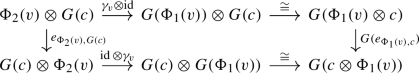
• an action coherence monoidal natural isomorphism $\gamma : \Phi _2\Rightarrow G\circ \Phi _1$ satisfying the following compatibility with the half-braidings:

  

Given two 1-morphisms $(G,\gamma ^G),(H,\gamma ^H)$ between pointed module tensor categories, by [HPT23b, Lem. 3.6], there is at most one monoidal natural transformation $\kappa : (G,\gamma ^G)\Rightarrow (H,\gamma ^H)$ satisfying the following compatibility with the action coherence morphisms:

When such a $\kappa$ exists, it is necessarily invertible. Hence the 2-category of pointed pivotal module tensor categories over $\mathcal {V}$ is 1-truncated, i.e., equivalent to a 1-category.

3.2 Unitary module tensor categories

For the remainder of this section, we assume that $(\mathcal {V},\vee _\mathcal {V})$ is a braided unitary tensor category with a fixed unitary dual functor, and let ${{\,\textrm{tr}\,}}^\mathcal {V}$ be the associated right pivotal trace.

Definition 3.4

Let $\mathcal {V}$ be as above. A unitary module (multi)tensor category over $\mathcal {V}$ is a unitary (multi)tensor category $\mathcal {C}$ with a unitary dual functor $\vee _\mathcal {C}$, a faithful state $\psi _\mathcal {C}$ on ${{\,\textrm{End}\,}}_\mathcal {C}(1_\mathcal {C})$, and a braided pivotal dagger tensor functor $\Phi ^{\scriptscriptstyle \mathcal {Z}} : \mathcal {V}\rightarrow \mathcal {Z}^\dag (\mathcal {C})$.

We call a unitary module multitensor category spherical if $\psi _\mathcal {C}$ is a spherical state (Definition 2.12). See Warning 2.15. Observe that, by Lemma 2.17, the existence of a non-zero spherical unitary $\mathcal {V}$-module tensor category implies that $\mathcal {V}$ is ribbon, i.e., that the unitary dual functor on $\mathcal {V}$ is spherical.

The choices of $\vee _\mathcal {C}$ and $\psi _\mathcal {C}$ endow $\mathcal {C}$ with a unitary trace

$$\begin{aligned} {{\,\textrm{Tr}\,}}^\mathcal {C}:=\psi _\mathcal {C}\circ {{\,\textrm{tr}\,}}^\vee _R. \end{aligned}$$

(15)

Moreover, $(\mathcal {C}, {{\,\textrm{Tr}\,}}^\mathcal {C})$ is a pivotal module $\textrm{C}^*$ category (aka unitary module category) [GMP+23, §3.6.2] for the underlying unitary tensor category of $\mathcal {V}$ (without the braiding). So unitary module tensor categories are, in particular, unitary module categories.

Remark 3.5

Suppose $(\mathcal {C},\vee _\mathcal {C},\psi _\mathcal {C},\Phi ^{\scriptscriptstyle \mathcal {Z}})$ is a unitary module multitensor category over $\mathcal {V}$. If $\Phi$ admits a right adjoint, then by Lemma 2.5, $\Phi$ admits a right unitary adjoint $\textbf{Tr}_\mathcal {V}$ which is automatically bi-involutive lax monoidal by Proposition 2.26 and Corollary 2.23. Thus $\textbf{Tr}_\mathcal {V}$ comes equipped with canonical unitary isomorphisms $\{\chi ^{\textbf{Tr}_\mathcal {V}}_c:\textbf{Tr}_\mathcal {V}({\overline{c}})\rightarrow \overline{\textbf{Tr}_\mathcal {V}(c)}\}_{c\in \mathcal {C}}$ satisfying the axioms in Definitions 2.20 and 2.25.

We warn the reader that ${{\,\textrm{Tr}\,}}^\mathcal {C}$ is a trace in the sense of Definition 2.1, whereas $\textbf{Tr}_\mathcal {V}$ is a categorified trace as described in Construction 3.2.

As before, a pointing of $\mathcal {C}$ is a choice of object $c\in \mathcal {C}$ such that c and $\Phi ^{\scriptscriptstyle \mathcal {Z}}(\mathcal {V})$ generate $\mathcal {C}$ under the operations of tensor product, orthogonal direct sum, and taking orthogonal direct summands. We also require that our symmetric self-duality $r_c: c\rightarrow c^\vee$ is unitary; this is also called a real structure for c.

Definition 3.6

A 1-morphism $(G,\gamma ): (\mathcal {C}_1,\vee _1,\psi _1,\Phi _1^{\scriptscriptstyle \mathcal {Z}},x_1) \rightarrow (\mathcal {C}_2,\vee _2,\psi _2,\Phi _2^{\scriptscriptstyle \mathcal {Z}},x_2)$ of pointed unitary module tensor categories over $\mathcal {V}$ is a 1-morphism of underlying pointed pivotal module tensor categories such that

• G is a $\dag$-tensor functor,

• the action coherence monoidal natural isomorphism $\gamma : \Phi _2 \Rightarrow G\circ \Phi _1$ is unitary and involutive: $\forall v\in \mathcal {V},\, \overline{\gamma _v} \circ \chi ^{\Phi _2}_v = \chi ^G_{\Phi _1(v)} \circ G(\chi ^{\Phi _1}_v)\circ \gamma _{{\overline{v}}}: \Phi _2({\overline{v}}) \rightarrow \overline{G(\Phi _1(v))}$,

• $\psi _2 \circ G = \psi _1$ on ${{\,\textrm{End}\,}}_{\mathcal {C}_1}(1_{\mathcal {C}_1})$.

3.3 The map $i^\dag$ and a formula for ${{\,\textrm{coev}\,}}^\dag _{\textbf{Tr}_\mathcal {V}(c)}$

In §4.3 below, we will define unitarity for an anchored planar algebra in terms of a certain pairing on $\mathcal {P}[n]$ from the anchored planar algebra being equal to ${{\,\textrm{coev}\,}}^\dag _{\mathcal {P}[n]}$.

Fix a unitary $\mathcal {V}$-module multitensor category $(\mathcal {C},\vee _\mathcal {C},\psi _\mathcal {C},\Phi ^{\scriptscriptstyle \mathcal {Z}})$ such that $\Phi : \mathcal {V}\rightarrow \mathcal {C}$ admits a right unitary adjoint $\textbf{Tr}_\mathcal {V}$. In this section, we will study $i^\dag :\textbf{Tr}_\mathcal {V}(1_\mathcal {C})\rightarrow 1_\mathcal {V}$, and prove the important formula (18) for ${{\,\textrm{coev}\,}}^\dag _{\textbf{Tr}_\mathcal {V}(c)}$. We represent $i^\dag$ diagrammatically by

In Lemma 3.11, we will show that if $\psi _\mathcal {C}$ is spherical, then all isotopies are allowed for strings on the capped tube:

Consider the finite dimensional abelian $\textrm{C}^{*}$-algebra $\mathcal {C}(1_\mathcal {C}\rightarrow 1_\mathcal {C})$. By unitary adjunction, we have an isomorphism

(16)

hence the right hand side is also equipped with the structure of an abelian $\textrm{C}^{*}$-algebra. The multiplication and $*$-structure on the right hand side of (16) are given by

$$\begin{aligned} x \cdot y = \mu _{1_\mathcal {C},1_\mathcal {C}}\circ (x\otimes y) \qquad \quad \text {and} \qquad \quad x^* = \big (\chi ^{\textbf{Tr}_\mathcal {V}}_{1_\mathcal {C}}\circ \textbf{Tr}_\mathcal {V}(r_\mathcal {C})\big )^{-1}\circ {\overline{x}}\circ r_\mathcal {V}. \end{aligned}$$

To see that the isomorphism (16) intertwines the two $*$-structures, i.e.,

$$\begin{aligned}&\textbf{Tr}_{\mathcal {V}}(f^\dag ) \circ i =(\chi _{1_{\mathcal {C}}}^{\textbf{Tr}_{\mathcal {V}}} \circ \textbf{Tr}_{\mathcal {V}}(r_{\mathcal {C}}))^{-1}\circ \overline{\textbf{Tr}_{\mathcal {V}}(f) \circ i } \circ r_{\mathcal {V}},{} & {} \text {equivalently}\\&\chi _{1_{\mathcal {C}}}^{\textbf{Tr}_{\mathcal {V}}} \circ \textbf{Tr}_{\mathcal {V}}(r_{\mathcal {C}}) \circ \textbf{Tr}_\mathcal {V}(f^\dag ) \circ i = \overline{ \textbf{Tr}_\mathcal {V}(f) \circ i } \circ r_\mathcal {V}, \end{aligned}$$

we check that, since $f^\dag ={\overline{f}}^{\vee }=(r_\mathcal {C})^{-1}\circ {\overline{f}}\circ r_\mathcal {C}$ on ${{\,\textrm{End}\,}}_\mathcal {C}(1_\mathcal {C})$ (as $r_\mathcal {C}={{\,\textrm{coev}\,}}_1$), we have

$$\begin{aligned} \chi _{1_{\mathcal {C}}}^{\textbf{Tr}_{\mathcal {V}}} \circ \textbf{Tr}_{\mathcal {V}}(r_{\mathcal {C}}) \circ \textbf{Tr}_{\mathcal {V}}(f^\dagger ) \circ i&= \chi _{1_{\mathcal {C}}}^{\textbf{Tr}_{\mathcal {V}}} \circ \textbf{Tr}_{\mathcal {V}}(r_{\mathcal {C}}) \circ \textbf{Tr}_\mathcal {V}(r_{\mathcal {C}}^{-1}) \circ \textbf{Tr}_\mathcal {V}({\overline{f}}) \circ \textbf{Tr}_\mathcal {V}(r_\mathcal {C})\circ i\\&=\chi _{1_{\mathcal {C}}}^{\textbf{Tr}_{\mathcal {V}}} \circ \textbf{Tr}_\mathcal {V}({\overline{f}}) \circ \textbf{Tr}_\mathcal {V}(r_\mathcal {C})\circ i\\&=\overline{\textbf{Tr}_\mathcal {V}(f)} \circ \chi _{1_{\mathcal {C}}}^{\textbf{Tr}_{\mathcal {V}}} \circ \textbf{Tr}_\mathcal {V}(r_\mathcal {C})\circ i\\&=\overline{\textbf{Tr}_\mathcal {V}(f)} \circ {\bar{i}} \circ r_\mathcal {V}. \end{aligned}$$

The third equality follows from involutivity of $\textbf{Tr}_\mathcal {V}$ (Definition 2.20), and the final equality uses the unitality axiom $\chi _{1_\mathcal {C}} \circ \textbf{Tr}(r_\mathcal {C}) \circ i = {\bar{i}} \circ r_\mathcal {V}$ from Definition 2.25, which holds by Proposition 2.26.

Lemma 3.7

The state $\mathcal {V}(1_\mathcal {V}\rightarrow \textbf{Tr}_\mathcal {V}(1_\mathcal {C})) \rightarrow {{\,\textrm{End}\,}}_\mathcal {V}(1_\mathcal {V})\cong \mathbb {C}$ given by $x\mapsto i^\dag \circ x$ corresponds to $\psi _\mathcal {C}:{{\,\textrm{End}\,}}_\mathcal {C}(1_\mathcal {C})\rightarrow \mathbb {C}$ under the isomorphism (16).

Proof

Fix $x\in \mathcal {V}(1_\mathcal {V}\rightarrow \textbf{Tr}_\mathcal {V}(1_\mathcal {C}))$. We then have

$$\begin{aligned} \psi _\mathcal {C}({{\,\textrm{mate}\,}}(x)) = \langle {{\,\textrm{mate}\,}}(x),{{\,\textrm{id}\,}}_{1_\mathcal {C}}\rangle _{1_\mathcal {C}\rightarrow 1_\mathcal {C}} = \langle x, i\rangle _{1_\mathcal {V}\rightarrow \textbf{Tr}_\mathcal {V}(1_\mathcal {C})} = i^\dag \circ x, \end{aligned}$$

where the first equality holds by combining (15) with the definition of $\langle \cdot \,,\cdot \rangle$ (Definition 2.1), and the second equality is the unitarity of the adjunction (16), using that ${{\,\textrm{mate}\,}}(i)={{\,\textrm{id}\,}}_{1_\mathcal {C}}$. $\square$

We will use the following lemma to get our equality of pairings in Proposition 3.9 below.

Lemma 3.8

Two maps $p,q: v\otimes {\overline{v}} \rightarrow 1_\mathcal {V}$ are equal if and only if for all $u\in \mathcal {V}$ and $f,g\in \mathcal {V}(u\rightarrow v)$,

$$\begin{aligned} p\circ (f\otimes {\overline{g}}) \circ {{\,\textrm{coev}\,}}_u = q\circ (f\otimes {\overline{g}}) \circ {{\,\textrm{coev}\,}}_u. \end{aligned}$$

(17)

Proof

The forward direction is trivial. Considering only simple $u\in {{\,\textrm{Irr}\,}}(\mathcal {V})$, the equality (17) holds iff

which holds true iff

$$\begin{aligned} p\circ (f\otimes {\overline{g}}) = q\circ (f\otimes {\overline{g}}) \qquad \qquad \forall \,f,g:u\rightarrow v. \end{aligned}$$

This is true for all u iff $p=q$. $\square$

Proposition 3.9

${{\,\textrm{coev}\,}}^\dag _{\textbf{Tr}_\mathcal {V}(c)}=i^\dag \circ \textbf{Tr}_\mathcal {V}({{\,\textrm{coev}\,}}^\dag _c)\circ \mu _{c,{\overline{c}}} \circ ({{\,\textrm{id}\,}}\otimes [\chi ^{\textbf{Tr}_\mathcal {V}}_c]^{-1}).$ Equivalently,

(18)

where we’ve suppressed the inverse of $\chi ^{\textbf{Tr}_\mathcal {V}}_c$ from the diagram.

Proof

Fix $v\in \mathcal {V}$, $f,g: v\rightarrow \textbf{Tr}_\mathcal {V}(c)$, and consider the morphism

(19)

Its mate under (16) is

$$\begin{aligned} \varepsilon _{1_\mathcal {C}} \circ \Phi (\textbf{Tr}_\mathcal {V}({{\,\textrm{coev}\,}}^\dag _c))\circ \Phi (\mu _{c,{\overline{c}}}) \circ \Phi \big (({{\,\textrm{id}\,}}_{\textbf{Tr}_\mathcal {V}(c)}\otimes (\chi ^{\textbf{Tr}_\mathcal {V}}_c)^{-1}) \circ (f\otimes {\overline{g}})\big )\circ \Phi ({{\,\textrm{coev}\,}}_v). \end{aligned}$$

We claim that the above morphism is equal to

$$\begin{aligned} {{\,\textrm{coev}\,}}^\dag _c \circ \big ({{{\,\textrm{mate}\,}}(f)} \otimes \overline{{{\,\textrm{mate}\,}}(g)}\big ) \circ {{\,\textrm{coev}\,}}_{\Phi (v)}. \end{aligned}$$

(20)

Indeed, in the diagrammatic notation of [HPT16], we check:

Now, by Lemma 3.7, $i^\dag \circ (19)=\psi _\mathcal {C}((20))$. By (15) and the definition of $\langle \cdot \,,\cdot \rangle$, this is equal to

$$\begin{aligned} \langle {{\,\textrm{mate}\,}}(f),{{\,\textrm{mate}\,}}(g)\rangle _{\mathcal {C}(\Phi (v)\rightarrow c)} =\langle f, g\rangle _{\mathcal {V}(v\rightarrow \textbf{Tr}(c))} ={{\,\textrm{tr}\,}}_\mathcal {V}(fg^\dag )={{\,\textrm{coev}\,}}^\dag _{\textbf{Tr}_\mathcal {V}(c)}\circ (f\otimes {\overline{g}})\circ {{\,\textrm{coev}\,}}_{v}. \end{aligned}$$

Hence

$$\begin{aligned} i^\dag \circ (19) = {{\,\textrm{coev}\,}}^\dag _{\textbf{Tr}_\mathcal {V}(c)}\circ (f\otimes {\overline{g}})\circ {{\,\textrm{coev}\,}}_{v} \qquad \qquad \forall \,f,g:v\rightarrow \textbf{Tr}_\mathcal {V}(c). \end{aligned}$$

The result follows by Lemma 3.8. $\square$

Remark 3.10

The problem of showing the pairing on the right hand side in the statement of Proposition 3.9 is non-degenerate was left open in [HPT16, Rem. 5.4]. As it is equal to ${{\,\textrm{coev}\,}}^\dag _{\textbf{Tr}_\mathcal {V}(c)}$ (up to suppressing $\chi$), this open question is now resolved in the unitary setting.

Lemma 3.11

If $\psi _\mathcal {C}$ is spherical, then the following maps $\textbf{Tr}_\mathcal {V}(c\otimes {\overline{c}})\rightarrow 1_\mathcal {V}$ are equal:

Note that the first and third tubes above represent the same morphism regardless of whether $\psi _\mathcal {C}$ is spherical or not, because the following two pictures are isotopic:

Proof

By the above discussion, it is enough to prove the first equality. Two maps $f,g:v\rightarrow 1_\mathcal {V}$ are equal if and only if $f\circ h = g\circ h$ for all $h: 1_\mathcal {V}\rightarrow v$, so we fix $h: 1_\mathcal {V}\rightarrow \textbf{Tr}_\mathcal {V}(c\otimes {\overline{c}})$ and wish to show that

(21)

By Lemma 3.7, this is the same as showing that

The result follows since

and

3.4 Unitarity of the traciator

Suppose $(\mathcal {C},\vee _\mathcal {C},\psi _\mathcal {C},\Phi ^{\scriptscriptstyle \mathcal {Z}})$ is a unitary module multitensor category over $\mathcal {V}$ and $\textbf{Tr}_\mathcal {V}:\mathcal {C}\rightarrow \mathcal {V}$ is the right unitary adjoint of $\Phi : \mathcal {V}\rightarrow \mathcal {C}$. Recall that each object $\Phi (v)$ comes with a unitary half-braiding $e_{\Phi (v),x}:\Phi (v)\otimes {x}\,\rightarrow \,{x}\otimes \Phi (v)$. In this section, we explore an extra coherence between these unitary half-braidings and the involutive structure of the categorified trace.

Lemma 3.12

We have the following coherence between the half-braiding $e_{\Phi (v),\bullet }$ and $\chi ^\Phi _v$:

Proof

Letting $(\overline{\Phi (v)},e_{\overline{\Phi (v)},\bullet })$ be the conjugate of $(\Phi (v),e_{\Phi (v),\bullet })$ in $Z^\dagger (\mathcal {C})$, we have $e_{\overline{\Phi (v)},b}=\nu _{b,\Phi (v)}^{-1} \circ \overline{e^{-1}_{\Phi (v),b}} \circ \nu _{\Phi (v),b}$, so the right hand side in the statement of the lemma simplifies to $e_{\overline{\Phi (v)},b}\circ (\chi ^\Phi _v \otimes {{\,\textrm{id}\,}}_{{\overline{b}}})$. (Note that since the half-braiding is unitary, we have $\overline{e^{-1}_{\Phi (v),b}}=e^\vee _{\Phi (v),b}$.) The result holds since $\chi ^\Phi _v: \Phi ({\overline{v}})\rightarrow \overline{\Phi (v)}$ is a morphism in $Z^\dag (\mathcal {C})$. $\square$

The following lemma expresses the coherence from Lemma 3.12 in terms of traciators.

Lemma 3.13

We have the following compatibility of the tracitator with the involutive structure of $\textbf{Tr}_\mathcal {V}$:

$$\begin{aligned} \overline{\tau _{x,y}} \circ \chi _{x\otimes y} \circ \textbf{Tr}_\mathcal {V}(\nu _{y,x}) = \chi _{y\otimes x} \circ \textbf{Tr}_\mathcal {V}(\nu _{x,y})\circ \tau _{{\overline{x}},{\overline{y}}}^{-1} \end{aligned}$$

(22)

Proof

We prove this equality after talking inverses on both sides, and after taking mates under the adjunction

$$\begin{aligned} \mathcal {V}\big (\overline{\textbf{Tr}_\mathcal {V}(y\otimes x)} \rightarrow \textbf{Tr}_\mathcal {V}({\overline{y}}\otimes {\overline{x}})\big ) \cong \mathcal {C}\big (\Phi (\overline{\textbf{Tr}_\mathcal {V}(y\otimes x)})\rightarrow {\overline{y}}\otimes {\overline{x}}\big ). \end{aligned}$$

The mate of the inverse of the left hand side of (22) is

$$\begin{aligned} {{\,\textrm{mate}\,}}(\textbf{Tr}_\mathcal {V}(\nu _{y,x}^{-1}) \circ \chi _{x\otimes y}^{-1}\circ \overline{\tau _{x,y}^{-1}})&= \nu _{y,x}^{-1} \circ {{\,\textrm{mate}\,}}(\chi _{x\otimes y}^{-1} ) \circ \Phi (\overline{\tau _{x,y}^{-1}}) \\ {}&= \nu _{y,x}^{-1}\circ \varepsilon _{\overline{x\otimes y}}\circ \Phi (\chi _{x\otimes y}^{-1})\circ \Phi (\overline{\tau _{x,y}^{-1}}) \\ {}&= \nu _{y,x}^{-1} \circ \overline{\varepsilon _{x\otimes y}} \circ \chi ^\Phi _{\textbf{Tr}_\mathcal {V}(x\otimes y)} \circ \Phi (\overline{\tau _{x,y}^{-1}}) \\ {}&= \nu _{y,x}^{-1} \circ \overline{\varepsilon _{x\otimes y}} \circ \overline{\Phi (\tau _{x,y}^{-1})} \circ \chi ^\Phi _{\textbf{Tr}_\mathcal {V}(y\otimes x)} \\ {}&= \nu _{y,x}^{-1} \circ \overline{\varepsilon _{x\otimes y} \circ \Phi (\tau _{x,y}^{-1})} \circ \chi ^\Phi _{\textbf{Tr}_\mathcal {V}(y\otimes x)} \\ {}&= \nu _{y,x}^{-1}\circ \overline{{{\,\textrm{mate}\,}}(\tau _{x,y}^{-1})} \circ \chi ^\Phi _{\textbf{Tr}_\mathcal {V}(y\otimes x)} \end{aligned}$$

where the third equality holds by the last equation in Proposition 2.21.

The mate of the inverse of the right hand side of (22) is ${{\,\textrm{mate}\,}}(\tau _{{\overline{x}},{\overline{y}}}) \circ \Phi (\textbf{Tr}_\mathcal {V}(\nu _{x,y}^{-1}))\circ \Phi (\chi _{y\otimes x}^{-1})$. Expanding, we get the map going right and then down in the pasting diagram below. To save space, we omit tensor symbols and subscripts.

It remains to prove that the map going down and then right in the above pasting diagram is equal to $\nu _{y,x}^{-1}\circ \overline{{{\,\textrm{mate}\,}}(\tau _{x,y}^{-1})} \circ \chi ^\Phi _{\textbf{Tr}_\mathcal {V}(y\otimes x)}$. Equivalently, we must show that

$$\begin{aligned} \overline{{{\,\textrm{mate}\,}}(\tau _{x,y}^{-1})} = \nu _{y,x}&\circ ({{\,\textrm{id}\,}}_{{\overline{y}}\otimes {\overline{x}}}\otimes {{\,\textrm{ev}\,}}_y) \circ ({{\,\textrm{id}\,}}_{{\overline{y}}}\otimes (\nu _{x,y}^{-1}\circ \overline{\varepsilon _{y\otimes x}})\otimes {{\,\textrm{id}\,}}_{y})\\&\circ ((\nu _{y, \Phi (\textbf{Tr}_\mathcal {V}(y\otimes x))}^{-1} \circ \overline{e^{-1}_{\Phi (\textbf{Tr}_\mathcal {V}(y\otimes x)),y}})\otimes {{\,\textrm{id}\,}}_y) \circ ({{\,\textrm{id}\,}}_{\overline{\Phi (\textbf{Tr}_\mathcal {V}(y\otimes x))}}\otimes {{\,\textrm{ev}\,}}_y^\dag ). \end{aligned}$$

By the coherences for $(\overline{\,\cdot \,},\nu )$, the above equality is equivalent to

$$\begin{aligned} {{\,\textrm{mate}\,}}(\tau _{x,y}^{-1}) = ({{\,\textrm{coev}\,}}_y^\dag \otimes {{\,\textrm{id}\,}}_{x\otimes y})&\circ ({{\,\textrm{id}\,}}_{{\overline{y}}}\otimes \varepsilon _{y\otimes x}\otimes {{\,\textrm{id}\,}}_y)\\&\circ ({{\,\textrm{id}\,}}_{{\overline{y}}}\otimes e^{-1}_{\Phi (\textbf{Tr}_\mathcal {V}(y\otimes x)),y}) \circ ({{\,\textrm{coev}\,}}_y \otimes {{\,\textrm{id}\,}}_{\Phi (\textbf{Tr}_\mathcal {V}(y\otimes x))}), \end{aligned}$$

which is exactly [HPT16, Lem. 4.14]. $\square$

In Jones’ planar algebras [Jon21], unitarity of the rotation plays a crucial role. Under the equivalence between anchored planar algebras and pivotal module tensor categories, the analog of rotation is given by the traciator. The next result says that traciators, and thus rotations in an anchored planar algebra, are unitary assuming sphericality.

Proposition 3.14

If the state $\psi _\mathcal {C}$ is spherical, then the traciator $\tau _{a,b}$ is unitary.

Proof

Since $\tau _{a,b}$ is invertible, it suffices to show that $\tau _{a,b}^\dag \tau _{a,b} = {{\,\textrm{id}\,}}_{\textbf{Tr}_\mathcal {V}(a\otimes b)}$. Since $\tau ^\dag = {\overline{\tau }}^\vee$, by Lemma 3.13 (and suppressing various coherences) we have $\tau ^\dagger =(\tau ^{-1})^\vee$. Thus:

$\square$

4 Unitary Anchored Planar Algebras

4.1 Planar algebras

We present here an abridged introduction to planar tangles, the planar operad, and planar algebras, and refer the reader to [HPT23b, §2.1] for an extended treatment.

An planar tangle consists of a collection of (round) parametrized disc $D_1,\ldots ,D_n$ inside some biger parametrised disc $D_0$, along with a collection of non-intersecting paths in $D_0\setminus (D_1\cup \ldots \cup D_k)$ called strings that start and end at the boundary of one of the circles, or are themselves closed loops. Here, a disc $D_i$ is called parametrised if $D_i=\varphi _i(\mathbb {D})$ for some chosen affine linear maps $\varphi _i:\mathbb {D}\rightarrow D_i$ from the standard unit disc. The points $\varphi _i(1)\in \partial D_i$ are called anchor points, and the strands are required to not start or end on the anchor points. Here is an example of a planar tangle, where we have marked the anchor points in red:

There is a composition operation for planar tangles

$$\begin{aligned} S\circ _i T := S \cup \phi _i(T) \end{aligned}$$

when the number of external string boundary points of T agrees with the number of internal string boundary points in the i-th disk of S. We shrink the tangle T, insert it into the i-th input disk of S using the map $\phi _i$, and match up the boundary points of the strings. For an explicit example, see [HPT23b, Ex. 2.2].

The collection of isotopy classes of planar tangles with the operation of tangle composition is called the planar operad. A planar algebra is an algebra for this operad. Unpacking, we have a vector space $\mathcal {P}[n]$ for each $n\in \mathbb {N}_{\ge 0}$, and each (isotopy class of) planar tangle T gives a linear map

Here, $n_i$ for $1\le i\le k$ is the number of boundary points of strings on the i-th input disk of T, and $n_0$ is the number of boundary points of strings on the output disk of T. For future convenience, we abbreviate these properties by saying T has type $(n_1,\dots , n_k; n_0)$.

Given planar tangles S, T of types $(m_1,\dots ,m_j;m_0), (n_1,\dots , n_k;n_0)$ respectively with $n_0=m_i$, composition of the linear maps Z(S), Z(T) must be compatible with composition of planar tangles:

$$\begin{aligned} Z(S\circ _i T)=Z(S)\circ ({{\,\textrm{id}\,}}_{\mathcal {P}[m_1]\otimes \ldots \otimes \mathcal {P}[m_{i-1}]}\otimes Z(T)\otimes {{\,\textrm{id}\,}}_{\mathcal {P}[m_{i+1}]\otimes \ldots \otimes \mathcal {P}[m_j]}). \end{aligned}$$

We also require that the identity tangle must act as the identity linear map. Finally, letting $T^\sigma$ be the tangle obtained by renumbering the input disks of T by some permutation $\sigma$, we should have $Z(T^\sigma )=Z(T)\circ \sigma$ (where we also use $\sigma$ to denote the symmetric braiding of the vector spaces $\mathcal {P}[n_i]$ corresponding to the permutation $\sigma$).

Remark 4.1

The notion of a planar algebra makes sense in any symmetric tensor category.

4.2 Anchored planar algebras

We present here an abridged introduction to the anchored planar operad and anchored planar algebras, and we refer the reader to [HPT23b, §2.2] for an extended treatment. An anchored planar tangle is a thing like this:

It differs from a planar tangle in that each internal anchor point is connected to the external anchor point by a red anchor line which stays in $D_0\setminus \{D_1,\ldots , D_k\}$. These anchor lines are transparent to the strings, but they may not intersect each other.

Like before, we say an anchored planar tangle T has type $(n_1,\dots , n_k; n_0)$ if T has k input disks, the i-th input disk of T meets $n_i$ string boundary points for $i\le 1\le k$, and the output disk of T meets $n_0$ string boundary points.

The anchored planar operad is the collection of isotopy classes of anchored planar tangles, with the operation of tangle composition. Here, given anchored planar tangles S, T of type $(m_1,\dots ,m_j;m_0), (n_1,\dots , n_k;n_0)$ respectively with $n_0=m_i$, the composition operation $S\circ _i T$ differs from the previous operation in that we must also give new anchor lines. We do so by replacing the i-th anchor line of T by k parallel lines, and composing each one of them with the i-th anchor line of S, as illustrated in the following picture:

(23)

Recall from [HPT16, Appendix A.2] that a braided pivotal tensor category is also rigid balanced.⁸ Hence our pivotal structure $\varphi ^\mathcal {V}$ induces a twist by

(24)

(By [HPT16, Prop. A.4], a braided unitary tensor category $(\mathcal {V},\beta ,\vee )$ is ribbon if and only if the $\varphi$ induced by $\vee$ is a spherical structure.)

Definition 4.2

Let $(\mathcal {V},\beta ,\varphi ^\mathcal {V})$ be a braided pivotal tensor category. An anchored planar algebra over $\mathcal {V}$ is an algebra in $\mathcal {V}$ over the anchored planar operad. Unpacking, we have a sequence $\mathcal {P}=(\mathcal {P}[n])_{n\ge 0}$ of objects of $\mathcal {V}$, along with operations

$$\begin{aligned} Z(T):\mathcal {P}[n_1]\otimes \ldots \otimes \mathcal {P}[n_k]\rightarrow \mathcal {P}[n_0] \end{aligned}$$

for every isotopy class of anchored planar tangle T of type $(n_1,\ldots ,n_k;n_0)$, subject to the following axioms:

• (identity) the identity anchored tangle acts as the identity morphism

• (composition) if S and T are anchored planar tangles of type $(m_1,\ldots ,m_j;m_0)$ and $(n_1,\ldots ,n_k;n_0)$, and if $n_0=m_i$, then

  $$\begin{aligned} Z(S\circ _i T)=Z(S)\circ ({{\,\textrm{id}\,}}_{\mathcal {P}[m_1]\otimes \ldots \otimes \mathcal {P}[m_{i-1}]}\otimes Z(T)\otimes {{\,\textrm{id}\,}}_{\mathcal {P}[m_{i+1}]\otimes \ldots \otimes \mathcal {P}[m_j]}) \end{aligned}$$

  (25)

• (anchor dependence) the following relations hold:

  • (braiding)     

  • (twist)          .

(Here, a little number n next to a string to indicates n parallel strings.) We call $\mathcal {P}[n]$ the n^th box object of the anchored planar algebra $\mathcal {P}$.

Notation 4.3

In the sections below, we use the notation of an anchored planar tangle T inserted into a coupon to denote the map Z(T) in $\mathcal {V}$ afforded by an anchored planar algebra. The strings in these diagrams are usually drawn horizontally for convenience, and we read them left to right. For example:

where T is the tangle in the coupon.

Definition 4.4

A morphism $H: \mathcal {P}_1\rightarrow \mathcal {P}_2$ of anchored planar algebras is a sequence of morphisms $(H[n]:\mathcal {P}_1[n]\rightarrow \mathcal {P}_2[n])_{n\ge 0}$ such that for every anchored planar tangle T of type $(n_1,\dots , n_k;n_0)$, $H[n_0]\circ Z(T) = Z(T)\circ (H[n_1]\otimes \cdots \otimes H[n_k])$.

4.3 Unitary anchored planar algebras

Let $(\mathcal {V},\vee ,\beta )$ be a unitary tensor category equipped with a chosen unitary dual functor $\vee$ and a unitary braiding $\beta = \{\beta _{u,v}: u\otimes v \rightarrow v\otimes u\}_{u,v\in \mathcal {V}}$ satisfying the usual axioms. Using the canonical pivotal structure (11) induced by $\vee$, the formula (24) for the twist simplifies to

Definition 4.5

A unitary anchored planar algebra in $\mathcal {V}$ is a triple $(\mathcal {P},r,\psi _\mathcal {P})$ consisting of an anchored planar algebra $\mathcal {P}$ in $\mathcal {V}$, a $\dag$-structure r, which is a family of real structures $r_n : \mathcal {P}[n] \rightharpoonup \mathcal {P}[n]$ for each $n\ge 0$, and a morphism $\psi _\mathcal {P}: \mathcal {P}[0] \rightarrow 1_\mathcal {V}$ called a faithful state satisfying such that:

• (P1) For every anchored planar tangle T of type $(n_1,\dots , n_k; n_0)$,

  $$\begin{aligned} \overline{Z(T)} \circ \nu ^{(k)}\circ (r_{n_k}\otimes \cdots \otimes r_{n_1})= r_{n_0}\circ Z({\overline{T}}), \end{aligned}$$

  where ${\overline{T}}$ is the reflection of T, and $\nu ^{(k)}: (\overline{\,\cdot \,}\otimes \ldots \otimes \overline{\,\cdot \,})\rightarrow \overline{(\,\cdot \,\otimes \cdots \otimes \,\cdot \,)}$ is an appropriate composite of $\nu$’s. When $k=0$, we have $\overline{Z(T)}\circ r_\mathcal {V}= r_{k_0}\circ Z({\overline{T}})$ where $r_\mathcal {V}: 1_\mathcal {V}\rightarrow \overline{1_\mathcal {V}}$ is the real structure of $1_\mathcal {V}$. (Suppressing the $\dag$-structure r, this axiom reads $Z({\overline{T}}) = \overline{Z(T)}$.)

• (P2) For every $n\ge 0$, we have an equality of pairings

  

  (26)

If $(\mathcal {V},\vee ,\beta )$ is moreover ribbon (so that $\vee$ is spherical), we say that a unitary anchored planar algebra $(\mathcal {P},r,\psi _\mathcal {P})$ is spherical if

In this paper, we do not always assume our anchored planar algebras to be spherical.

Definition 4.6

A morphism $H: (\mathcal {P}_1,r^1,\psi _1) \rightarrow (\mathcal {P}_2,r^2,\psi _2)$ of unitary anchored planar algebras is a morphism H of anchored planar algebras satisfying $\overline{H[n]}\circ r^1_n = r^2_n\circ H[n]$ for all $n\ge 0$, and $\psi _1 = \psi _2\circ H[0]$.

When $\mathcal {V}=\textsf{Hilb}_{\textsf{fd}}$, the definition of unitary anchored planar algebra reduces to the definition of a unitary planar algebra (also known as a semisimple $\textrm{C}^{*}$ planar algebra) from [GMP+23], but equipped with a faithful state. (The planar algebra of a bipartite graph [Jon00] is an example of a $\textrm{C}^{*}$ planar algebra that is naturally equipped wiht a faithful state.)

The following lemma is straightfoward and left to the reader.

Lemma 4.7

If a unitary anchored planar algebra is spherical, then for every $n\ge 0$ we have

$\square$

Proposition 4.8

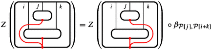
Let $(\mathcal {P},r,\psi _\mathcal {P})$ be a spherical unitary anchored planar algebra. Let A be an annular anchored planar tangle, and denote the inside-out reflection by $A^\dag$. Then $Z(A)^\dag =Z(A^\dag )$.

Corollary 4.9

is unitary.

Proof

Suppose A has m input strings and n output strings. Since $\psi _\mathcal {P}$ is spherical, the morphism

Indeed, this can be checked directly using sphericality of $\psi _\mathcal {P}$ by writing A as a composite of generating annular anchored planar tangles (see §5.1 below), and ‘pulling them over’ one at a time. By (26), the above equality simplifies (after a 90$^\circ$ rotation of the string diagrams) to

Precomposing with ${{\,\textrm{id}\,}}\otimes {{\,\textrm{ev}\,}}_{\mathcal {P}[m]}^\dag$, we get the desired equality

$\square$

5 Extending the Equivalence

We now prove Theorem A, extending the equivalence from [HPT23b, Thm. A] to an equivalence

$$\begin{aligned} \left\{ \begin{array}{l} \mathrm{Unitary\, anchored\, planar\,} \\ \mathrm{algebras\, in\, } \mathcal {V}\end{array} \right\} \,\,\,\,\cong \,\, \left\{ \begin{array}{l} \mathrm{Pointed\, unitary\, module\, multitensor} \\ \mathrm{categories\, over} \mathcal {V}\, \end{array} \right\} \end{aligned}$$

Recall that, by definition (see §3.2), a unitary module multitensor category comes with a state $\psi _\mathcal {C}$ and requires that the $\mathcal {V}$-action $\Phi ^{\scriptscriptstyle Z}:\mathcal {V}\rightarrow Z^{\dag }(\mathcal {C})$ is pivotal.

5.1 From unitary module tensor categories to unitary anchored planar algebras

Let $(\mathcal {C},\Phi ^{\scriptscriptstyle \mathcal {Z}},\vee _\mathcal {C},\psi _\mathcal {C})$ be a pointed unitary module multitensor category over $\mathcal {V}$, with real generator $(x,r_x)\in \mathcal {C}$, and $\textbf{Tr}_\mathcal {V}:\mathcal {C}\rightarrow \mathcal {V}$ the unitary right adjoint of $\Phi = {{\,\textrm{Forget}\,}}_\mathcal {Z}\circ \Phi ^{\scriptscriptstyle \mathcal {Z}}:\mathcal {V}\rightarrow \mathcal {C}$. We may then construct an ordinary anchored planar algebra, as in [HPT23b, Thm. 5.1]. This anchored planar algebra is completely determined by the following information:

• $\mathcal {P}[n]:=\textbf{Tr}_\mathcal {V}(x^{\otimes n})$

• 
• 
• 
• 

5.1.1 Adding the dagger structure

It remains to construct the $\dag$-structure r and the state $\psi _\mathcal {P}$ on $\mathcal {P}$, satisfying the conditions listed in Definition 4.5.

Definition 5.1

For $n\ge 0$, we define $r_n : \mathcal {P}[n]\rightarrow \overline{\mathcal {P}[n]}$ to be the composite

$$\begin{aligned} \textbf{Tr}_\mathcal {V}(x^{\otimes n}) \xrightarrow {\textbf{Tr}_\mathcal {V}(r_x^{\otimes n})} \textbf{Tr}_\mathcal {V}({\overline{x}}^{\otimes n}) \xrightarrow {\textbf{Tr}_\mathcal {V}(\nu )} \textbf{Tr}_\mathcal {V}(\overline{x^{\otimes n}}) \xrightarrow {\chi ^{\textbf{Tr}_\mathcal {V}}_{x^{\otimes n}}} \overline{\textbf{Tr}_\mathcal {V}(x^{\otimes n})}. \end{aligned}$$

Lemma 5.2

$\overline{r_n}\circ r_n = \varphi _{\mathcal {P}[n]}$.

Proof

Going right and then down in the following commutative diagram is $\overline{r_n}\circ r_n$

This is equal to the curved arrow $\varphi _{\textbf{Tr}_\mathcal {V}(x^{\otimes n})}=\varphi _{\mathcal {P}[n]}$. $\square$

Proposition 5.3

The pair $(\mathcal {P},r)$ satisfies P1:

$$\begin{aligned} \overline{Z(T)}\circ \nu ^{(k)} \circ (r_{n_k}\otimes \cdots \otimes r_{n_1}) = r_{n_0}\circ Z({\overline{T}}). \end{aligned}$$

(When $k=0$, $\overline{Z(T)}\circ r_\mathcal {V}= r_{n_0}\circ Z({\overline{T}})$ where $r_\mathcal {V}: 1_\mathcal {V}\rightarrow \overline{1_\mathcal {V}}$ is the real structure of $1_\mathcal {V}$.)

Proof

This essentially follows from the fact that $\textbf{Tr}_\mathcal {V}$ is involutive lax monoidal by Proposition 2.26. It is enough to check P1 on each of the following generating tangles:

First, since ${\overline{u}}=u$, by unitality,

$$\begin{aligned} \overline{Z(u)}\circ r_\mathcal {V}= {\overline{i}} \circ r_\mathcal {V}= \chi ^{\textbf{Tr}_\mathcal {V}}_1 \circ \textbf{Tr}_\mathcal {V}(r_\mathcal {C}) \circ i = r_0\circ Z({\overline{u}}). \end{aligned}$$

Since $\overline{m_{i,j}}=m_{j,i}$, by monoidality,

$$\begin{aligned} \overline{Z(m_{i,j})}\circ \nu \circ (r_j\otimes r_i)&= \overline{\mu _{i,j}}\circ \nu \circ \big ( (\chi ^{\textbf{Tr}_\mathcal {V}}_{x^{\otimes j}}\circ \textbf{Tr}_\mathcal {V}(\nu )\circ \textbf{Tr}_\mathcal {V}(r_x^{\otimes j}))\\&\quad \otimes (\chi ^{\textbf{Tr}_\mathcal {V}}_{x^{\otimes i}}\circ \textbf{Tr}_\mathcal {V}(\nu )\circ \textbf{Tr}_\mathcal {V}(r_x^{\otimes i})) \big )\\&=\overline{\mu _{i,j}}\circ \nu \circ (\chi ^{\textbf{Tr}_\mathcal {V}}_{x^{\otimes j}}\otimes \chi ^{\textbf{Tr}_\mathcal {V}}_{x^{\otimes i}}) \circ (\textbf{Tr}_\mathcal {V}(\nu )\otimes \textbf{Tr}_\mathcal {V}(\nu ))\\&\quad \circ (\textbf{Tr}_\mathcal {V}(r_x^{\otimes j})\otimes \textbf{Tr}_\mathcal {V}(r_x^{\otimes i}))\\&= \chi ^{\textbf{Tr}_\mathcal {V}}_{x^{\otimes i+j}} \circ \textbf{Tr}_\mathcal {V}(\nu ) \circ \mu _{\overline{x^{\otimes j}},\overline{x^{\otimes i}}} \circ (\textbf{Tr}_\mathcal {V}(\nu )\otimes \textbf{Tr}_\mathcal {V}(\nu )) \\&\quad \circ (\textbf{Tr}_\mathcal {V}(r_x^{\otimes j})\otimes \textbf{Tr}_\mathcal {V}(r_x^{\otimes i}))\\&= \chi ^{\textbf{Tr}_\mathcal {V}}_{x^{\otimes i+j}} \circ \textbf{Tr}_\mathcal {V}(\nu ) \circ \textbf{Tr}_\mathcal {V}(r_x^{\otimes i+j}) \circ \mu _{j,i}\\&= r_{i+j}\circ Z(\overline{m_{i,j}}). \end{aligned}$$

The third equality above uses the lax involutive property of $\textbf{Tr}_\mathcal {V}$, and the fourth equality uses naturality of $\mu$. Since $\overline{a_i}=a_{n-i}$ (when $Z(a_i):\textbf{Tr}_\mathcal {V}(x^{\otimes n+2})\rightarrow \textbf{Tr}_\mathcal {V}(x^{\otimes n})$), we see

$$\begin{aligned} \overline{Z(a_i)} \circ r_{n+2}&= \overline{\textbf{Tr}_\mathcal {V}({{\,\textrm{id}\,}}_{x^{\otimes i}} \otimes {{\,\textrm{ev}\,}}_x \otimes x^{\otimes n-i})} \circ \chi ^{\textbf{Tr}_\mathcal {V}}_{x^{\otimes n+2}} \circ \textbf{Tr}_\mathcal {V}(\nu ) \circ \textbf{Tr}_\mathcal {V}(r_x^{\otimes n+2}) \\ {}&= \chi ^{\textbf{Tr}_\mathcal {V}}_{x^{\otimes n}} \circ \textbf{Tr}_\mathcal {V}(\nu ) \circ \textbf{Tr}_\mathcal {V}(r_x^{\otimes n}) \circ \textbf{Tr}_\mathcal {V}({{\,\textrm{id}\,}}_{x^{\otimes n-i}} \otimes {{\,\textrm{ev}\,}}_x \otimes x^{\otimes i}) = r_n\circ Z(a_{n-i}). \end{aligned}$$

The proof for the $a_i^\dag$ is similar and omitted. (It also follows formally from the proof for $a_i$ as $\textbf{Tr}_\mathcal {V}$ is a dagger functor and $\chi ^{\textbf{Tr}_\mathcal {V}}$, r, $\nu$, and $r_x$ are all unitary.) Finally, for the tangles $t_{i,j}$, we have $\overline{t_{i,j}}=t_{i,j}^{-1}$, and by Lemma 3.13,

$$\begin{aligned} \overline{Z(t_{i,j})}\circ r_n&= \overline{\tau _{i,j}} \circ \chi ^{\textbf{Tr}_\mathcal {V}}_{x^{\otimes n}} \circ \textbf{Tr}_\mathcal {V}(\nu ) \circ \textbf{Tr}_\mathcal {V}(r_x^{\otimes n}) \\ {}&= \chi ^{\textbf{Tr}_\mathcal {V}}_{x^{\otimes n}} \circ \textbf{Tr}_\mathcal {V}(\nu ) \circ \tau ^{-1}_{{\overline{x}}^{\otimes i},{\overline{x}}^{\otimes j}} \circ \textbf{Tr}_\mathcal {V}(r_x^{\otimes n}) \\ {}&= \chi ^{\textbf{Tr}_\mathcal {V}}_{x^{\otimes n}} \circ \textbf{Tr}_\mathcal {V}(\nu ) \circ \textbf{Tr}_\mathcal {V}(r_x^{\otimes n}) \circ \tau ^{-1}_{x^{\otimes i},x^{\otimes j}} \\ {}&= r_n \circ Z(\overline{t_{i,j}}). \end{aligned}$$

$\square$

Definition 5.4

We define a state $\psi _\mathcal {P}:=i^\dag : \mathcal {P}[0] \rightarrow 1_\mathcal {V}$ as in §3.3.

Proposition 5.5

The triple $(\mathcal {P},r,\psi _\mathcal {P})$ satisfies P2.

Proof

Suppressing $\chi ^{\textbf{Tr}_\mathcal {V}}$ and $\nu$,

$\square$

Proposition 5.6

If $\psi _\mathcal {C}$ is spherical,⁹ so is $\psi _\mathcal {P}$.

Proof

If $\psi _\mathcal {C}$ is spherical, then

$\square$

5.1.2 Functoriality

Suppose $G=(G,\gamma ): (\mathcal {C}_1,\Phi _1^{\scriptscriptstyle \mathcal {Z}},\vee _1,\psi _1,x_1) \rightarrow (\mathcal {C}_2,\Phi _2^{\scriptscriptstyle \mathcal {Z}},\vee _2,\psi _2,x_2)$ is a 1-morphism of pointed unitary module multitensor categories over $\mathcal {V}$. (Recall that $\gamma$ is a family of unitary isomorphisms $\gamma _v: \Phi _2(v)\rightarrow G(\Phi _1(v))$.)

Let $(\mathcal {P}_i,r^i,\psi _i)=\Lambda (\mathcal {C}_i,\Phi _i^{\scriptscriptstyle \mathcal {Z}},\vee _i,\psi _i,x_i)$ be the unitary anchored algebra constructed in the previous subsection for $i=1,2$. In [HPT23b, §5.3], we obtained a map of ordinary anchored planar algebras $\Lambda (G): \mathcal {P}_1\rightarrow \mathcal {P}_2$ as follows.

• First, for each $c\in \mathcal {C}_1$, we define $\zeta _c : \textbf{Tr}_\mathcal {V}^1(c) \rightarrow \textbf{Tr}_\mathcal {V}^2(G(c))$ to be the mate of

  $$\begin{aligned} \Phi _2(\textbf{Tr}_\mathcal {V}^1(c)) \xrightarrow {\gamma _{\textbf{Tr}_\mathcal {V}^1(c)}} G(\Phi _1(\textbf{Tr}_\mathcal {V}^1(c))) \xrightarrow {G(\varepsilon _c^1)} G(c) \end{aligned}$$

  under the unitary adjunction $\Phi _2 \dashv \textbf{Tr}_\mathcal {V}^2$.

• The map $\Lambda (G):\mathcal {P}_1\rightarrow \mathcal {P}_2$ associated to $G:(\mathcal {C}_1, x_1)\rightarrow (\mathcal {C}_2, x_2)$ is the sequence of morphisms $\Lambda (G)[n]:\mathcal {P}_1[n]\rightarrow \mathcal {P}_2[n]$ given by

  $$\begin{aligned} \Lambda (G)[n]\,:\,\mathcal {P}_1[n] = \textbf{Tr}_\mathcal {V}^1(x_1^{\otimes n}) \xrightarrow {\,\,\,\,\textstyle \zeta _{x_1^{\otimes n}}\,\,\,} \textbf{Tr}_\mathcal {V}^2(G(x_1^{\otimes n})) \xrightarrow {\cong } \textbf{Tr}_\mathcal {V}^2(x_2^{\otimes n}) = \mathcal {P}_2[n]. \end{aligned}$$

It remains to prove that $\Lambda (G)$ is compatible with $r_n$ and $\psi$, i.e.,

$$\begin{aligned} \overline{\Lambda (G)[n]}\circ r_n^1&= r_n^2\circ \Lambda (G)[n]{} & {} \forall \,n\ge 0 \end{aligned}$$

(27)

$$\begin{aligned} \text {and}\quad \psi _1&= \psi _2\circ \Lambda (G)[0]. \end{aligned}$$

(28)

Equation (27) is checked by the following commutative diagram.

Lemma 5.7

The natural transformation $\zeta : \textbf{Tr}_\mathcal {V}^1 \Rightarrow \textbf{Tr}_\mathcal {V}^2\circ G$ is involutive, i.e., for all $c\in \mathcal {C}_1$, $\overline{\zeta _c}\circ \chi ^{\textbf{Tr}_\mathcal {V}^1}_{c} = \chi ^{\textbf{Tr}_\mathcal {V}^2}_{G(c)}\circ \textbf{Tr}_\mathcal {V}^2(\chi ^G_c) \circ \zeta _{{\overline{c}}}$.

Proof

We prove the equivalent relation:

$$\begin{aligned} (\chi ^{\textbf{Tr}_\mathcal {V}^2}_{G(c)})^{-1}\circ \overline{\zeta _c} = \textbf{Tr}_\mathcal {V}^2(\chi ^G_c) \circ \zeta _{{\overline{c}}}\circ (\chi ^{\textbf{Tr}_\mathcal {V}^1}_{c})^{-1}. \end{aligned}$$

To do so, we take mates under the adjunction

$$\begin{aligned} \mathcal {V}(\overline{\textbf{Tr}_\mathcal {V}^1(c)}\rightarrow \textbf{Tr}_\mathcal {V}^2(\overline{G(c)})) \cong \mathcal {C}_1(\Phi _2(\overline{\textbf{Tr}_\mathcal {V}^1(c)})\rightarrow \overline{G(c)}). \end{aligned}$$

In the commutative diagram below, the mate of the left hand side above is going down and then right, and the mate of the right hand side is going right and then down.

The pentagon in the diagram above is the involutivity axiom for $\gamma$. $\square$

Checking (28) is straightforward. By Lemma 3.7, $\psi _j$ on ${{\,\textrm{End}\,}}_{\mathcal {C}_j}(1_{\mathcal {C}_j})$ is identified with $i_j^\dag \circ -$ on ${{\,\textrm{Hom}\,}}_\mathcal {V}(1\rightarrow \mathcal {P}_j[0])$ under the isomorphism (16), which is exactly $\psi _j$ on $\mathcal {P}_j$ by Definition 5.4. Since $\psi _1=\psi _2 \circ G$ on ${{\,\textrm{End}\,}}_{\mathcal {C}_1}(1_{\mathcal {C}_1})$, the result follows.

5.2 From unitary anchored planar algebras to unitary module tensor categories

Given a unitary anchored planar algebra $(\mathcal {P},r,\psi _\mathcal {P})$ in $\mathcal {V}$, we begin by constructing an ordinary pivotal module tensor category $(\mathcal {C},\Phi ^{\scriptscriptstyle \mathcal {Z}})$ as in [HPT23b, §6]. First, we construct a full subcategory $\mathcal {C}_0$, and we obtain $\mathcal {C}$ by taking the Cauchy completion.

• Objects in $\mathcal {C}_0$ are formal symbols $``\Phi (v)\otimes x^{\otimes n}"$ for $v\in \mathcal {V}$ and $n\ge 0$.

• Hom spaces are defined by

  $$\begin{aligned} \mathcal {C}_0(``\Phi (u)\otimes x^{\otimes k}" \rightarrow ``\Phi (v)\otimes x^{\otimes n}") := \mathcal {V}(u \rightarrow v\otimes \mathcal {P}[n+k]). \end{aligned}$$

  Morphisms are represented graphically by

• Composition is given by

  

• The adjoint functor pair $\Phi \dashv \textbf{Tr}_\mathcal {V}$ is given on objects by $\Phi (u):=``\Phi (u)\otimes x^{\otimes 0}"$ and $\textbf{Tr}_\mathcal {V}(``\Phi (v)\otimes x^{\otimes n}"):=v\otimes \mathcal {P}[n]$ and given on morphisms by

  

  Moreover, the identity map

  $$\begin{aligned} \mathcal {C}\big (\Phi (u)\rightarrow ``\Phi (v)\otimes x^{\otimes n}"\big ) = \mathcal {V}\big (u\rightarrow v\otimes \mathcal {P}[n]\big ) = \mathcal {V}\big (u\rightarrow \textbf{Tr}_\mathcal {V}(``\Phi (v)\otimes x^{\otimes n}")\big ) \end{aligned}$$

  witnesses the adjunction $\Phi \dashv \textbf{Tr}_\mathcal {V}$.

• Tensor product is given by

  

  and the tensor unit is given by $``\Phi (1)\otimes x^{\otimes 0}"$. The associators and unitors are inhereted from those of $\mathcal {V}$, i.e.,

  

  and similarly for the unitors $\lambda ,\rho$.

• $\mathcal {C}_0$ is rigid with duals given by $(``\Phi (v)\otimes x^{\otimes n}")^\vee :=``\Phi (v^\vee )\otimes x^{\otimes n}"$, and evaluation and coevaluation given by

  

  Note here that the evaluation and coevaluation in $\mathcal {V}$ come from our chosen unitary dual functor of $\mathcal {V}$. These choices of duals endow $\mathcal {C}_0$ with a dual functor $\vee _\mathcal {C}$.

• The pivotal structure $\varphi ^\mathcal {C}:``\Phi (v)\otimes x^{\otimes n}"\rightarrow (``\Phi (v)\otimes x^{\otimes n}")^{\vee \vee }$ is given by

  

  The equality above comes from the fact that $\varphi _v$ is the canonical unitary pivotal structure of $\mathcal {V}$ coming from $\vee$.

• The generator is $x=``\Phi (1_\mathcal {V})\otimes x"$. Since we identify $1_\mathcal {V}^\vee$ with $1_\mathcal {V}$, we may identify $x^\vee =x$. The symmetric self duality $r_x:x\rightarrow x^\vee$ is the identity map.

5.2.1 Adding the dagger structure

It remains to perform the following tasks:

• (C1) construct a dagger structure on $\mathcal {C}$ making it a unitary multitensor category

• (C2) construct a faithful state $\psi _\mathcal {C}$ on ${{\,\textrm{End}\,}}_\mathcal {C}(1_\mathcal {C})$,

• (C3) check that $\vee _\mathcal {C}$ is a unitary dual functor and that the canonical unitary pivotal structure induced by $\vee _\mathcal {C}$ is $\varphi ^\mathcal {C}$.

• (C4) check that $r_x:x\rightarrow x^\vee$ is a real structure.

• (C5) check that the adjunction $\Phi \dashv \textbf{Tr}_\mathcal {V}$ is unitary.

Definition 5.8

We define a dagger structure on $\mathcal {C}_0$ by

(29)

It is straightforward to verify that $f^{**}=f$ for all morphisms f. To check the remainder of involutivity, we see that $*$ on the composite

$$\begin{aligned} ``\Phi (u)\otimes x^{\otimes k}" \xrightarrow {f} ``\Phi (v)\otimes x^{\otimes n}" \xrightarrow {g} ``\Phi (w)\otimes x^{\otimes p}" \end{aligned}$$

is given by

which is exactly the composite of $f^*$ and $g^*$. We now observe that

where we use the braiding axiom of an anchored planar algebra in the final equality. Finally, the associators and unitors are visibly unitary.

Lemma 5.9

For all $f\in \mathcal {C}_0(``\Phi (u)\otimes x^{\otimes k}" \rightarrow ``\Phi (v)\otimes x^{\otimes n}")$,

with equality if and only if $f=0$.

Proof

Expanding the quantity in question, we have

with equality if and only if $f=0$. $\square$

Proposition 5.10

[(C1)] The dagger structure (29) on $\mathcal {C}_0$ is $\textrm{C}^{*}$.

Proof

To show $\mathcal {C}_0$ is $\textrm{C}^{*}$, we prove that given arbitrary $``\Phi (u)\otimes x^{\otimes k}"$ and $``\Phi (v)\otimes x^{\otimes n}"$ in $\mathcal {C}_0$, the linking algebra

$$\begin{aligned} L:= \begin{pmatrix} \mathcal {C}_0(``\Phi (u)\otimes x^{\otimes k}" \rightarrow ``\Phi (u)\otimes x^{\otimes k}") &{} \mathcal {C}_0(``\Phi (v)\otimes x^{\otimes n}" \rightarrow ``\Phi (u)\otimes x^{\otimes k}") \\ \mathcal {C}_0(``\Phi (u)\otimes x^{\otimes k}" \rightarrow ``\Phi (v)\otimes x^{\otimes n}") &{} \mathcal {C}_0(``\Phi (v)\otimes x^{\otimes n}" \rightarrow ``\Phi (v)\otimes x^{\otimes n}") \end{pmatrix} \end{aligned}$$

is a $\textrm{C}^{*}$-algebra. To do this, we show that the map $\phi :L\rightarrow \mathbb {C}$ given by

is a faithful positive linear functional, i.e., $\phi (M^*M)\ge 0$ with equality if and only if $M=0$. Indeed, $\phi (M^*M)$ is a sum of four terms, each being positive by Lemma 5.9, and zero iff each term is individually zero. $\square$

Remark 5.11

Observe that the unitary Cauchy completion of $\mathcal {C}_0$ is the same as the ordinary Cauchy completion of $\mathcal {C}_0$ [GMP+23, Rem. 3.6]. In light of Proposition 5.10, $\mathcal {C}$ is a unitary multitensor category.

Corollary 5.12

[(C2)] The map $\psi _\mathcal {C}$ on ${{\,\textrm{End}\,}}_{\mathcal {C}_0}(1_\mathcal {C})$ given by

is a faithful state.

Proof

Apply Lemma 5.9 to the case $u=v=1_\mathcal {V}$ and $k=n=0$ to see that $\psi _\mathcal {C}$ is positive and faithful. Finally, the condition $\psi _\mathcal {C}({{\,\textrm{id}\,}}_{\mathcal {C}})=1$ is exactly . $\square$

Proposition 5.13

[(C3)] The dual functor $\vee _\mathcal {C}$ is unitary. Moreover, the pivotal structure $\varphi ^\mathcal {C}$ is the canonical unitary pivotal structure coming from $\vee _\mathcal {C}$.

Proof

By [Sel11, Lem. 7.5] (see also [Pen20, Prop. 3.9]), it suffices to check that for $c:=``\Phi (v)\otimes x^{n}"$, the pivotal structure $\varphi ^\mathcal {C}_c$ above is given by $({{\,\textrm{coev}\,}}_c^\dag \otimes {{\,\textrm{id}\,}}_{c^{\vee \vee }})\circ ({{\,\textrm{id}\,}}_c\otimes {{\,\textrm{coev}\,}}_{c^\vee })$. This is verified as follows. First, we observe that

We then calculate with $c=``\Phi (v)\otimes x^{n}"$ that $({{\,\textrm{coev}\,}}_c^\dag \otimes {{\,\textrm{id}\,}}_{c^{\vee \vee }})\circ ({{\,\textrm{id}\,}}_c\otimes {{\,\textrm{coev}\,}}_{c^\vee })$ is given by

This completes the proof. $\square$

Corollary 5.14

[(C4)] The symmetric self-duality $r_x: x\rightarrow x^\vee$ is unitary, i.e., $(x,r_x)$ is real.

Proof

We used the identification between $1_\mathcal {V}^\vee = 1_\mathcal {V}$ to identify $x=x^\vee$ and $r_x = {{\,\textrm{id}\,}}_x$, but the former identification is unitary, so the latter is too. $\square$

Recall from Lemma 2.17 that sphericality of the unitary dual functor $\vee _\mathcal {V}$ is a necessary condition for the state $\psi _\mathcal {C}$ to be spherical.

Proposition 5.15

If $\vee _\mathcal {V}$ is a spherical unitary dual functor on $\mathcal {V}$ and $(\mathcal {P},j,\psi _\mathcal {P})$ is spherical, then so is $\psi _\mathcal {C}$.

Proof

For $f\in {{\,\textrm{End}\,}}_{\mathcal {C}_0}(``\Phi (u)\otimes x^{\otimes n}")$, its left and right traces in $\mathcal {C}$ are given by

Now since $\vee _\mathcal {V}$ and $\psi _\mathcal {P}$ are spherical, we see that

and thus $\psi _\mathcal {C}({{\,\textrm{tr}\,}}^\mathcal {C}_L(f))=\psi _\mathcal {C}({{\,\textrm{tr}\,}}^\mathcal {C}_R(f))$. $\square$

Now that $\mathcal {C}_0$ is endowed with a unitary dual functor and faithful state, we get a unitary trace on ${{\,\textrm{End}\,}}_{\mathcal {C}_0}(``\Phi (v)\otimes x^{\otimes n}")$ by $\psi _\mathcal {C}\circ {{\,\textrm{tr}\,}}^\mathcal {C}_R$.

Proposition 5.16

[(C5)] The adjunction $\Phi \dashv \textbf{Tr}_\mathcal {V}$ is unitary. In particular, $\Phi$ and $\textbf{Tr}_\mathcal {V}$ are dagger functors.

Proof

We show the two inner products on $\mathcal {V}\big (u\rightarrow v\otimes \mathcal {P}[n]\big )$ coming from $\mathcal {C}$ and $\mathcal {V}$ agree:

as in the proof of Lemma 5.9. $\square$

5.2.2 Functoriality

We now suppose $H: (\mathcal {P}_1,r^1,\psi _1)\rightarrow (\mathcal {P}_2,r^2,\psi _2)$ is a map of unitary anchored planar algebras, and let $(\mathcal {C}_i,\Phi _i^{\scriptscriptstyle \mathcal {Z}},\vee _i,\psi _i,x_i)=\Delta (\mathcal {P}_i)$ for $i=1,2$ be the pointed unitary module multitensor categories constructed in the last subsection. In [HPT23b, §6.6], we constructed a strict map of ordinary pointed pivotal module tensor categories $\Delta (H): \mathcal {C}_1\rightarrow \mathcal {C}_2$ by

where the action-coherence morphism $\gamma ^{\Delta (H)}: \Phi _2\Rightarrow \Delta (H)\circ \Phi _1$ is the identity.

It remains to prove that:

• $\Delta (H)$ is a $\dag$-tensor functor,

• the identity action coherence monoidal natural isomorphism ${{\,\textrm{id}\,}}: \Phi _2 \Rightarrow \Delta (H)\circ \Phi _1$ is involutive, i.e., for all $v\in \mathcal {V}$, $\chi ^{\Phi _2}_v = \chi ^{\Delta (H)}_{\Phi _1(v)}\circ \Delta (H)(\chi ^{\Phi _1}_v): \Phi _2({\overline{v}}) \rightarrow \overline{\Delta (H)(\Phi _1(v))}$, and

• $\psi _2 \circ \Delta (H) = \psi _1$ on ${{\,\textrm{End}\,}}_{\mathcal {C}_1}(1_{\mathcal {C}_1})$.

For the first condition, since $\Delta (H)$ is strict, it suffices to check it is a $\dag$-functor. Indeed,

For the second condition, since these are the canonical coherences $\chi$ associated to a strict pivotal $\dag$-tensor functor, they are all identities, and the result holds trivially.

Finally, for the third condition, for all $f\in {{\,\textrm{End}\,}}_{\mathcal {C}_1}(1_{\mathcal {C}_1})$,

5.3 Equivalence

Fix a braided unitary tensor category $\mathcal {V}$ with a choice of unitary dual functor $\vee _\mathcal {V}$. For this section, we use the following notation.

• $\textsf{APA}$ is the 1-category of anchored planar algebras over $\mathcal {V}$, and $\textsf{UAPA}$ is the 1-subcategory of unitary anchored planar algebras over $\mathcal {V}$.

• $\textsf{ModTens}$ is the 1-truncation of the 2-category of pointed pivotal module tensor categories over $\mathcal {V}$, and $\textsf{UModTens}$ is the 1-truncation of the 2-category of pointed unitary module multitensor categories over $\mathcal {V}$.

In [HPT23b], we constructed functors $\Delta : \textsf{APA}\rightarrow \textsf{ModTens}$ and $\Lambda : \textsf{ModTens}\rightarrow \textsf{APA}$. In §5.2.2 above, we showed $\Delta$ extends to a functor $\textsf{UAPA}\rightarrow \textsf{UModTens}$, and in §5.1.2 above, we showed $\Lambda$ extends to a functor $\textsf{UModTens}\rightarrow \textsf{UAPA}$. Moreover, these extensions are clearly compatible with the forgetful functors which forget our extra unitary structure.

In [HPT23b, §7], we showed that $\Lambda \circ \Delta ={{\,\textrm{id}\,}}_{\textsf{APA}}$, and it is immediate that $\Lambda \circ \Delta ={{\,\textrm{id}\,}}_{\textsf{UAPA}}$ upstairs. We also constructed a natural isomorphism $\Psi : \Delta \circ \Lambda \Rightarrow {{\,\textrm{id}\,}}_{\textsf{ModTens}}$

where $\mathcal {C}'=\Lambda (\Delta (\mathcal {C}))$, which is the unitary Cauchy completion of $\mathcal {C}'_0$ (recall $\mathcal {C}_0'$ has objects $``\Phi (v)\otimes x^{\otimes n}"$ for $v\in \mathcal {V}$).

It remains to show that $\Psi$ lifts to a unitary natural isomorphism upstairs. To do so, it is enough (in view of the fact that $\Psi$ is an isomorphism) to show that $f\mapsto \Psi (f)$ is norm-preserving, i.e.,

$$\begin{aligned} \big \Vert f\big \Vert _{\mathcal {V}(u\rightarrow v\otimes \mathcal {P}[i+j])} = \big \Vert \Psi (f)\big \Vert _{\mathcal {C}(\Phi (u)\otimes x^{\otimes i} \rightarrow \Phi (v)\otimes x^{\otimes j})}. \end{aligned}$$

By replacing f by ${{\,\textrm{ev}\,}}_v\circ (1_{{{\overline{v}}}}\otimes f)$ (i.e. folding the v strand to the left), we may assume without loss of generality that $v=1_\mathcal {V}$. Similarly, by replacing $f\in \mathcal {C}'\big (``\Phi (u)\otimes x^{\otimes i}" \rightarrow ``\Phi (v)\otimes x^{\otimes j}"\big )$ by the corresponding morphism in $\mathcal {C}'\big (``\Phi (u)\otimes x^{\otimes 0}" \rightarrow ``\Phi (v)\otimes x^{\otimes i+j}"\big )$, we may assume without loss of generality that $i=0$. We may now proceed as in the proof of Proposition 3.9 to show:

as desired.

References

Aasen, D., Lake, E., Walker, K.: Fermion condensation and super pivotal categories. J. Math. Phys. 60(12), 121901 (2019). https://doi.org/10.1063/1.5045669. arXiv:1709.01941
Baez, J.C.: Higher-dimensional algebra. II. \(2\)-Hilbert spaces. Adv. Math. 127(2), 125–189 (1997). https://doi.org/10.1006/aima.1997.1617
Bischoff, M. , Charlesworth, I. , Evington, S.,Giorgetti, L. , Penneys, D.: Distortion for multifactor bimodules and representations of multifusion categories, 2020. arXiv:2010.01067
Baez, J.C., Dolan, J.: Higher-dimensional algebra and topological quantum field theory. J. Math. Phys. 36(11), 6073–6105 (1995). https://doi.org/10.1063/1.531236. arXiv:q-alg/9503002
Bartels, A., Douglas, C.L., Henriques, A.: Dualizability and index of subfactors. Quantum Topol. 5(3), 289–345 (2014). https://doi.org/10.4171/QT/53. arXiv:1110.5671
Bion-Nadal, J.: An example of a subfactor of the hyperfinite \({\rm II}_1\) factor whose principal graph invariant is the Coxeter graph \(E_6\). In Current topics in operator algebras (Nara, 1990), pages 104–113. World Sci. Publ., River Edge, NJ, 1991
Chen, Q., Hernández Palomares, R., Jones, C., Penneys, D.: Q-system completion for \(\rm C^*\) 2-categories. J. Funct. Anal. 283(3), 109524 (2022). https://doi.org/10.1016/j.jfa.2022.109524. arXiv:2105.12010
Chen, Q., Penneys, D.: Q-system completion is a 3-functor. Theory Appl. Categ. 38, 101–134 (2022). https://doi.org/10.1002/num.22828. arXiv:2106.12437
Décoppet, T.D.: Multifusion categories and finite semisimple 2-categories. J. Pure Appl. Algebra 226(8), 16 (2022). https://doi.org/10.1016/j.jpaa.2022.107029. arXiv:2012.15774
Dell, Z., Huston, P., Penneys, D.: Unitary braided-enriched monoidal categories, 2022. arXiv:2208.14992
Douglas, C.L., R.D.J.: Fusion 2-categories and a state-sum invariant for 4-manifolds, (2018). arXiv:1812.11933
Egger, J.M.: On involutive monoidal categories. Theory Appl. Categ. 25(14), 368–393 (2011)
Etingof, P., Gelaki, S., Nikshych, D., Ostrik, V.: Tensor categories, volume 205 of Mathematical Surveys and Monographs. American Mathematical Society, Providence, RI, (2015) https://doi.org/10.1090/surv/205
Goodman, F.M., Harpe, P.d., Jones, V.F.R.: Coxeter graphs and towers of algebras. Mathematical Sciences Research Institute Publications, 14. Springer-Verlag, New York, 1989. x+288 pp. ISBN: 0-387-96979-9,
Gaiotto, D., Johnson-Freyd, T.: Condensations in higher categories, 2019. arXiv:1905.09566
Ghez, P., Lima, R., Roberts, J.E.: \(W^\ast \)-categories. Pacific J. Math. 120(1), 79–109 (1985)
Grossman, P., Morrison, S., Penneys, D., Peters, E., Snyder, N.:. The Extended Haagerup fusion categories. Ann. Sci Éc Norm Supér. 56(2):589–664, (2023). https://doi.org/10.24033/asens.2541arXiv:1810.06076
Huston, P., Burnell, F., Jones, C., Penneys, D.: Composing topological domain walls and anyon mobility. SciPost Phys., 15(3):85, 2023. https://doi.org/10.21468/SciPostPhys.15.3.076arXiv:2208.14018
Henriques, A.: Bicommutant categories from conformal nets, 2017. arXiv:1701.02052
Henriques, A.G.: What Chern-Simons theory assigns to a point. Proc. Natl. Acad. Sci. USA, 114(51):13418–13423, 2017. https://doi.org/10.1073/pnas.1711591114arXiv:1503.06254
Henriques, A., Penneys, D.: Bicommutant categories from fusion categories. Selecta Math. 23(3), 1669–1708 (2017). https://doi.org/10.1007/s00029-016-0251-0. arXiv:1511.05226
Henriques, A., Penneys, D.: Representations of fusion categories and their commutants. Selecta Math. 29(3), 38 (2023). https://doi.org/10.1007/s00029-023-00841-2. arXiv:2004.08271
Henriques, A., Penneys, D., Tener, J.: Categorified trace for module tensor categories over braided tensor categories. Doc. Math. 21, 1089–1149 (2016). arXiv:1509.02937
Henriques, A., Penneys, D. Tener, J.: Classification of finite depth objects in bicommutant categories via anchored planar algebras. (2023) arXiv:2307.13822
Henriques, A., Penneys, D., Tener, J.: Planar algebras in braided tensor categories. Mem. Am. Math. Soc. (2023). https://doi.org/10.1090/memo/1392. arXiv:1607.06041
Heunen, C., Vicary, J.: Categories for quantum theory, volume 28 of Oxford Graduate Texts in Mathematics. Oxford University Press, Oxford, 2019. An introduction, https://doi.org/10.1093/oso/9780198739623.001.0001
Izumi, M.: On flatness of the Coxeter graph \(E_8\). Pacific J. Math. 166(2), 305–327 (1994)
Johnson-Freyd, T.: On the classification of topological orders. Comm. Math. Phys. 393(2), 989–1033 (2022). https://doi.org/10.1007/s00220-022-04380-3. arXiv:2003.06663
Jaffe, A., Liu, Z.: Planar Para Algebras, Reflection Positivity. Comm. Math. Phys. 352(1), 95–133 (2017). https://doi.org/10.1007/s00220-016-2779-4. arXiv:1602.02662
Vaughan, F.R.: Jones. Index for subfactors. Invent. Math. 72(1), 1–25 (1983). https://doi.org/10.1007/BF01389127
Jones, V.F.R.: The planar algebra of a bipartite graph. In: Knots in Hellas ’98 (Delphi), volume 24 of Ser. Knots Everything, pp. 94–117. World Sci. Publ, River Edge, NJ (2000)
Jones, V.F.R.: Planar algebras, I. New Zealand J. Math., 52:1–107, (2021). https://doi.org/10.53733/172arXiv:math.QA/9909027
Jones, C., Penneys, D.: Operator algebras in rigid \(\rm C^*\)-tensor categories. Comm. Math. Phys. 355(3), 1121–1188 (2017). https://doi.org/10.1007/s00220-017-2964-0. arXiv:1611.04620
Jones, C., Penneys, D.: Q-systems and compact W*-algebra objects. In Topological phases of matter and quantum computation, volume 747 of Contemp. Math., pages 63–88. Amer. Math. Soc., Providence, RI, 2020. https://doi.org/10.1090/conm/747/15039arXiv:1707.02155
Kawahigashi, Y.: On flatness of Ocneanu’s connections on the Dynkin diagrams and classification of subfactors. J. Funct. Anal. 127(1), 63–107 (1995). https://doi.org/10.1006/jfan.1995.1003
Kelly, G.M.: Doctrinal adjunction. In Category Seminar (Proc. Sem., Sydney, 1972/1973), pages 257–280. Lecture Notes in Math., Vol. 420. Springer, Berlin, 1974
Longo, R. Roberts, J.E.: A theory of dimension. \(K\)-Theory, 11(2):103–159, 1997. https://doi.org/10.1023/A:1007714415067arXiv:funct-an/9604008
Lurie, J.: On the classification of topological field theories. In Current developments in mathematics, 2008, pages 129–280. Int. Press, Somerville, MA, 2009. arXiv:0905.0465
Penneys, D.: Unitary dual functors for unitary multitensor categories. High. Struct., 4(2):22–56, 2020. arXiv:1808.00323
Popa, S.: Classification of subfactors: the reduction to commuting squares. Invent. Math. 101(1), 19–43 (1990). https://doi.org/10.1007/BF01231494
Popa, S.: Classification of subfactors and their endomorphisms, volume 86 of CBMS Regional Conference Series in Mathematics. Published for the Conference Board of the Mathematical Sciences, Washington, DC, 1995
Selinger, P.: A survey of graphical languages for monoidal categories. In New structures for physics, volume 813 of Lecture Notes in Phys., pages 289–355. Springer, Heidelberg, 2011. https://doi.org/10.1007/978-3-642-12821-9_4
Tomatsu, R.: Centrally Free Actions of Amenable \(\rm C^*\)-tensor categories on von Neumann algebras. Comm. Math. Phys. 383(1), 71–152 (2021). https://doi.org/10.1007/s00220-021-04037-7. arXiv:1812.04222
Yamagami, S.: Frobenius duality in \(C^*\)-tensor categories. J. Operator Theory 52(1), 3–20 (2004)
Acknowledgements
The authors would like to thank Peter Huston and David Reutter for helpful conversations. David Penneys was supported by NSF DMS 1500387/1655912, 1654159, and 2154389. James Tener was supported by Australian Research Council Discovery Project DP200100067, as well as by the Max Planck Institute for Mathematics, Bonn, during the initial stages of this work.
Author information
Authors and Affiliations
Corresponding author
Additional information
Communicated by Y. Kawahigash.
Publisher's Note
Springer Nature remains neutral with regard to jurisdictional claims in published maps and institutional affiliations.
Rights and permissions
Open Access This article is licensed under a Creative Commons Attribution 4.0 International License, which permits use, sharing, adaptation, distribution and reproduction in any medium or format, as long as you give appropriate credit to the original author(s) and the source, provide a link to the Creative Commons licence, and indicate if changes were made. The images or other third party material in this article are included in the article's Creative Commons licence, unless indicated otherwise in a credit line to the material. If material is not included in the article's Creative Commons licence and your intended use is not permitted by statutory regulation or exceeds the permitted use, you will need to obtain permission directly from the copyright holder. To view a copy of this licence, visit http://creativecommons.org/licenses/by/4.0/.
About this article
Cite this article
Henriques, A., Penneys, D. & Tener, J. Unitary Anchored Planar Algebras. Commun. Math. Phys. 405, 137 (2024). https://doi.org/10.1007/s00220-024-04985-w
Received:
Accepted:
Published:
DOI: https://doi.org/10.1007/s00220-024-04985-w