Algebraic Conditions for Conformal Superintegrability in Arbitrary Dimension

Abstract

We consider second order (maximally) conformally superintegrable systems and explain how the definition of such a system on a (pseudo-)Riemannian manifold gives rise to a conformally invariant interpretation of superintegrability. Conformal equivalence in this context is a natural extension of the classical (linear) Stäckel transform, originating from the Maupertuis-Jacobi principle. We extend our recently developed algebraic geometric approach for the classification of second order superintegrable systems in arbitrarily high dimension to conformally superintegrable systems, which are presented via conformal scale choices of second order superintegrable systems defined within a conformal geometry. For superintegrable systems on constant curvature spaces, we find that the conformal scales of Stäckel equivalent systems arise from eigenfunctions of the Laplacian and that their equivalence is characterised by a conformal density of weight two. Our approach yields an algebraic equation that governs the classification under conformal equivalence for a prolific class of second order conformally superintegrable systems. This class contains all non-degenerate examples known to date, and is given by a simple algebraic constraint of degree two on a general harmonic cubic form. In this way the yet unsolved classification problem is put into the reach of algebraic geometry and geometric invariant theory. In particular, no obstruction exists in dimension three, and thus the known classification of conformally superintegrable systems is reobtained in the guise of an unrestricted univariate sextic. In higher dimensions, the obstruction is new and has never been revealed by traditional approaches.

1 Introduction

Transformation groups play an important role in the natural sciences: the Poincaré group, for instance, and its subgroups, are pivotal in special relativity, for Maxwell’s field equations, in particle physics, and many other fields. Felix Klein’s Erlangen program has put the concept of transformations at the core of geometry, later generalised by Cartan [Kle00, SC00]. Inspired by this idea, the current paper reconsiders second order superintegrable Hamiltonian systems. These have been extensively studied as structures in (pseudo-)Riemannian geometry, but not yet as structures in conformal geometry.

Maximally superintegrable systems, traditionally, are Hamiltonian systems on a (pseudo-) Riemannian geometry that admit a maximal amount of (hidden) symmetry. Here second order maximally (conformally) superintegrable systems are exclusively considered. They are often seminal models in science. Historically, the theory of superintegrability arose from classical (and quantum) mechanics: While, in general, it is impossible, even for relatively simple models, to solve Hamilton’s or Schrödinger’s equation in exact, closed terms, for superintegrable systems the solution can be found by quadrature, i.e. using algebraic operations and the integration of known functions. Prominent examples of second order superintegrable systems are the Kepler-Coulomb and the Harmonic oscillator models. They have fundamental significance for the understanding of celestial mechanics, atomic orbitals, material science and many other disciplines.

1.1 What Geometry underpins superintegrability?

Traditionally, second order superintegrable systems are defined on a (pseudo-)Riemannian manifold (M, g). The suitable symmetry group for these systems is the semi-direct product $\mathfrak S=\textrm{Diff}(M)\rtimes \textrm{Aff}({\mathbb {R}})$ of diffeomorphisms (coordinate transformations on M) and the affine group $\textrm{Aff}({\mathbb {R}})={\mathbb {R}}^*\ltimes {\mathbb {R}}$, where ${\mathbb {R}}^*={\mathbb {R}}\setminus \{0\}$, see Sect. 2. However, these are not the only possible transformations of superintegrable systems. Indeed, conformal geometry manifests itself in the theory of superintegrable systems through (classical) Stäckel equivalence or coupling constant metamorphosis; details and a comparison with the more recent concept of non-linear multi-parameter Stäckel transform are discussed in Sect. 2.1. Historically, the Stäckel transform can be traced back to the 18^th centrury in the form of the Maupertuis principle [Tsi01, BKF95, Lag88, Jac84, dM50]. Classical Stäckel transformations are linked to very special conformal transformations, namely those that originate from superintegrable potentials.

Arbitrary conformal transformations, however, do not preserve superintegrability. Instead they lead to conformally superintegrable systems. Although these systems are well studied, their underlying conformal geometry is understood only superficially to date. One purpose of the present paper is to remedy this, and to derive a suitable concept of conformal equivalence on conformally superintegrable systems from (a modification of) Stäckel equivalence.

Given the significance of second order (conformally) superintegrable systems, it is natural to seek a classification. In [KSV23], the authors present an algebraic geometric framework for a classification of second order superintegrable systems in arbitrarily high dimension, and for arbitrary metrics. This framework put earlier attempts by various authors (see below) onto a firm base, yet it is not closed under conformal transformations of superintegrable systems. The current paper develops an algebraic geometric framework for conformally superintegrable systems that is closed under conformal transformations. In particular we obtain: Non-degenerate second order (conformally) superintegrable systems are characterised by a (conformally invariant) structure tensor, more specifically a trace-free and totally symmetric tensor field $S_{ijk}$. This leads to a natural definition of superintegrability on conformal manifolds, whose symmetry group we identify as $\mathfrak S=\textrm{Conf}(M)\rtimes {\mathbb {R}}^*$. In this way we naturally incorporate conformal geometry into the theory of superintegrable systems. Somewhat surprisingly, this appears to never have been attempted before, although it sheds considerable light on the geometry underpinning superintegrability and opens the subject for subsequent studies using Cartan geometry, tractor calculus, algebraic geometry, representation theory and geometric invariant theory. In particular, superintegrable systems on (pseudo-) Riemannian geometries can be viewed as specific conformal scale choices of a conformally invariant superintegrable system.

1.2 State of the art

A vast literature exists both on second order conformally superintegrable systems and on Stäckel transformations. To date, second order conformally superintegrable systems are classified completely only in dimension 2 [KKM05c, KKM05a]. For conformally flat spaces in dimension 3, at least so-called non-degenerate systems are classified [Cap14, KKM06]. The conformal classes of non-degenerate systems are classified in dimensions 2 and 3 [Kre07, Cap14]. Existing classification results largely ignore the geometric structure of the classification space. However, an algebraic geometric classification exists for superintegrable systems in the Euclidean plane [KS18], and the algebraic varieties of superintegrable systems in dimensions 2 and 3 are addressed in [KKM07a, KKM07b]. While the classification of the conformal classes in dimension 2 is a mere list [Kre07], in dimension 3 a classification in terms of representations of the rotation group exists [Cap14, CK14, CKP15]. These latter references are one major inspiration for our work as they highlight the power of the geometric approach, revealing for example a natural algebraic hierarchy of systems related to an inclusion tree of certain algebraic ideals. Unfortunately, there is little hope of applying the methods from those references in higher dimensions, neither conceptually nor practically, as the equations become ever more extensive with increasing dimension. The current paper develops a new approach, extending and generalising the framework from [KS18, KSV23]. We formulate the governing equations for second order conformally superintegrable systems in dimension $n\geqslant 3$ in a concise form, making the problem manageable in higher dimensions.

Stäckel transformations can be traced back to Maupertuis-Jacobi transformations [Jac84], which take a Hamiltonian with potential to a potential-free one. The classical Stäckel transform is well understood as an equivalence relation on second order (conformally) superintegrable systems. It was first introduced, for integrable Hamiltonian systems with potential, in [HGDR84] under the name coupling constant metamorphosis. The name Stäckel transformations has been introduced in [BKM86] for transformations of integrable systems admitting separation of variables. In general, coupling constant metamorphosis and (classical) Stäckel transform are not identical, but they coincide for second order (conformal) integrals of the motion [Pos10]. Higher order integrals are discussed in [KMP09], showing that coupling constant metamorphosis in general does not even preserve the polynomiality in momenta of an integral. The classical Stäckel transform involves one parameter on which the Hamiltonian depends linearly. A multi-parameter generalisation of Stäckel transform was developed in [SB08, BM12, BM17], allowing for several parameters on which the Hamiltonian may depend non-linearly. Here we only encounter Hamiltonians with linear parameter dependence, and therefore we do not need to exhaust the full scope of generalised multi-parameter Stäckel transformations. As we are interested in a geometric approach, we shall not require a specific parametrisation of the space of compatible potentials, but instead work with an $(n+2)$-dimensional linear space of potentials on an n-dimensional manifold, usually not specifying a particular basis.

For completeness we mention that conformal transformations are not the only possible transformations of superintegrable systems. For instance, Bôcher transformations of certain conformally superintegrable systems are studied in [KMS16, CKP15] and there is some indication that they can be understood as boundaries of orbit closures on the algebraic variety classifying the superintegrable systems [KS18]. Yet another transformation of superintegrable systems is possible if the underlying metrics share the same geodesics up to reparametrisation. Such metrics are called projectively (or geodesically) equivalent. For some examples of superintegrable systems defined on projectively equivalent geometries, see [Val16, KKMW03, Vol20].

To summarise, higher dimensions are out of the scope of traditional methods, which rely on the correspondence with properly superintegrable systems and on the extensive use of computer algebra. A particular challenge is the fast growth of the number of partial differential equations with increasing dimension. In the current paper, we overcome this problem and outline how to approach the classification of second order conformally superintegrable systems in arbitrarily high dimension. For the most prolific class of systems we find, somewhat surprisingly, that the underlying structure equations reduce to only a single, algebraic equation of degree 2.

1.3 Classifying second order superintegrability in arbitrarily high dimension

In reference [KSV23] the authors have developed an algebraic geometric framework for the classification of superintegrable systems. This framework generalises previous work in dimension two [KS18] to arbitrarily high dimensions. Older works in the field are [KKM07a] and [KKM07b] for dimensions two and three, respectively. While [KSV23] for the first time provides a framework to classify, in an algebraic geometric way, superintegrable systems in arbitrarily high dimensions, this framework in its original form is not (yet) closed under conformal transformations. The present paper extends the existing algebraic geometric framework to conformally superintegrable systems on (pseudo-) Riemannian metrics. This new framework is closed under conformal transformations.

Second order conformally superintegrable systems will be thoroughly introduced in Sects. 3.1 and 3.2. These systems are traditionally defined using a Hamiltonian

$$\begin{aligned} H = g^{ij}({\textbf{q}})p_ip_j+V({\textbf{q}}) \end{aligned}$$

(1.1)

where $g_{ij}$ denotes the underlying metric and where ${\textbf{q}}$ and ${\textbf{p}}$ are the canonical position and momenta variables on the manifold. A second order conformally superintegrable system is a Hamiltonian system with a sufficiently high number of functions $F:T^*M\rightarrow {\mathbb {R}}$, $F=K^{ij}({\textbf{q}})p_ip_j+W({\textbf{q}})$, satisfying

$$\begin{aligned} \{ H,F \} = \omega _q({\textbf{p}})\,H \end{aligned}$$

(1.2)

for some 1-form $\omega =\omega _idx^i$. The scalar function V is called a potential of H. Functions F satisfying (1.2) are called (conformal) integrals. The integrals F form a linear space ${\mathcal {F}}$. Likewise, the potentials V compatible with ${\mathcal {F}}$ form a linear space ${\mathcal {V}}$. Following the common convention, we take these spaces to be maximal, see Definitions 2.2 and 3.5 below.

1.4 First main result: conformal superintegrability in higher dimensions

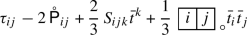
The method carried out in [KSV23] facilitates the classification of second order properly superintegrable systems, in particular of so-called abundant systems. Abundantness is going to be introduced thoroughly later, and so here we limit ourselves to saying that these systems comprise all known non-degenerate second order conformally superintegrable systems. In the present paper, we extend the framework to conformally superintegrable systems. We find that it is closed under conformal transformations and leads to a well-defined concept of superintegrability on conformal geometries arising from conformal equivalence classes of conformally superintegrable systems. For the abundant case in dimensions $n\geqslant 3$, we show in Sects. 5 and 6 that such systems are in natural correspondence with harmonic cubic forms $\Psi _{ijk}p^i\!p^j\!p^k$ on ${\mathbb {R}}^n$ that satisfy the simple algebraic equation

$$\begin{aligned} \left( g^{ab}\Psi _{{ija}}\Psi _{klb} - g^{ab}\Psi _{{ika}}\Psi _{jlb} \right) _\circ = 0 \end{aligned}$$

(1.3)

where $g^{ab}$ is an inner product on ${\mathbb {R}}^n$ with the same signature as the metrics on the underlying manifold. The subscript “$\circ$” stands for projection onto the trace-free part.

We show that initial data in the form of a cubic form $\Psi _{ijk}p^i\!p^j\!p^k$ satisfying (1.3) can be extended, locally, to a conformal structure tensor $S_{ijk}$ of an abundant second order superintegrable system. We make this precise by introducing the concept of c-superintegrable systems, i.e. conformal equivalence classes whose underlying geometry is a conformal manifold. In Sect. 6.4 we derive conformally invariant structural equations for abundant c-superintegrable systems. The equations governing abundant properly superintegrable systems [KSV23] naturally follow from the equations we present here. Condition (1.3) is conformally invariant, and therefore a suitable foundation for an algebraic geometric classification of second order systems on the level of conformal geometries. Condition (1.3) is also surprisingly simple, and in dimensions $n\geqslant 4$ it encodes new obstructions to conformal superintegrability. These obstructions do not exist in lower dimensions and have not been revealed by classical approaches.

We also show: Abundant conformally superintegrable systems can only exist on conformally flat geometries. Such systems naturally correspond to solutions of Eq. (1.3). The task of classifying equivalence classes of n-dimensional conformally superintegrable systems is therefore equivalent to classifying harmonic cubics in n variables that satisfy (1.3). Note that while a general classification of harmonic cubics under the rotation group is out of sight, a classification under the additional condition (1.3) may well be simple enough to admit a managable solution.

In dimension $n=3$, particularly, (1.3) is trivially satisfied. Thus abundant superintegrable systems in dimension 3 naturally correspond to harmonic ternary cubic forms, or, equivalently, to univariate sextic polynomials

$$\begin{aligned} p(x) = a_6x^6 + a_5x^5 + a_4x^4 + a_3x^3 + a_2x^2 + a_1x + a_0. \end{aligned}$$

The details are discussed in Sect. 7. It is known that any conformally superintegrable system is Stäckel equivalent to a properly superintegrable systems [Cap14]. In dimension 3, every conformally superintegrable system is even Stäckel equivalent to a properly superintegrable system on a constant curvature space [KKM06, Theorem 4].

1.5 Second main result: superintegrable systems on constant curvature geometries

In our framework, second order conformally superintegrable systems are conformal scale choices of c-superintegrable systems. Thus the conformal structure tensor $S_{ijk}$ determines a conformally superintegrable system up to the choice of a conformal scale expressed via a function $\sigma$ that transforms as a weight-1 tensor density. For the prolific class of abundant second order conformally superintegrable systems we find that the conformal scale satisfies a Helmholtz like equation,

$$\begin{aligned} \left( R-4\frac{n-1}{n-2}\Delta \right) \sigma ^{1-\tfrac{n}{2}} = S\,\sigma ^{1-\tfrac{n}{2}}\,, \end{aligned}$$

(1.4)

where $S=S_{abc}S^{abc}$ is a conformal density obtained from the structure tensor $S_{ijk}$ mentioned earlier, and where R is the scalar curvature. The operator on the left hand side of (1.4) is the conformal Laplace operator.

If we restrict to properly superintegrable systems, the conformal structure tensor $S_{ijk}$ determines a superintegrable system up to provision of a suitable conformal scale. In the present paper, we prove the following: For abundant properly superintegrable systems on manifolds of constant sectional curvature, the conformal scale $\sigma$ is (a power of) an eigenfunction of the Laplacian for an eigenvalue determined by the curvature R,

$$\begin{aligned} \Delta \,\sigma ^{n+2} = -2\frac{n+1}{n-1}\,R\,\sigma ^{n+2}\,, \end{aligned}$$

(1.5)

which holds in addition to (1.4), see Theorem 6.11. Note that the operator in (1.5) is not conformally invariant as Eq. (1.5) does not describe a property of the conformal class, but of an individual superintegrable system. In particular we find that on the n-sphere the conformal scale function satisfies a Laplace equation with quantum number $n+1$. We show for any dimension (see Propositions 6.14 and 6.15): The generic system on the n-sphere is never conformally equivalent to a superintegrable system on flat space, and a non-degenerate properly superintegrable system on the n-sphere is never conformally equivalent to the harmonic oscillator.

2 Preliminaries

Before generalising to conformally superintegrable systems, it is instructive to briefly review properly superintegrable systems. We recall that, for clarity, the adjective “proper” is used to refer to superintegrable systems, whenever a distinction from conformally superintegrable systems is required. While self-contained, this review only highlights the aspects needed for a later comparison to conformally superintegrable systems. For a more in-depth review of proper superintegrability we refer the interested reader to the literature cited in the introduction and in particular to [KKM18].

Let (M, g) be a (pseudo-) Riemannian manifold. A Hamiltonian system on M is a dynamical system characterised by a function $H:T^*M\rightarrow {\mathbb {R}}$, $({\textbf{p}},{\textbf{q}})\mapsto H({\textbf{p}},\textbf{q})$, referred to as Hamiltonian. We denote the position and momentum coordinates on the phase space $T^*M$ by $\textbf{q}=(q_1,\ldots ,q_n)$ and ${\textbf{p}}=(p_1,\ldots ,p_n)$, respectively. The evolution of the system is determined by Hamilton’s equations

$$\begin{aligned} \dot{{\textbf{p}}}&=-\frac{\partial H}{\partial {\textbf{q}}}&\dot{{\textbf{q}}}&=+\frac{\partial H}{\partial {\textbf{p}}}\,. \end{aligned}$$

(2.1)

An integral, aka first integral or constant of the motion, for the Hamiltonian H is a function $F(\textbf{p},{\textbf{q}})$ on phase space that commutes with H with respect to the canonical Poisson bracket. It is therefore constant along solutions of (2.1),

$$\begin{aligned} \dot{F} = \{F,H\} = \frac{\partial F}{\partial {\textbf{q}}}\,\frac{\partial H}{\partial {\textbf{p}}} - \frac{\partial F}{\partial {\textbf{p}}}\,\frac{\partial H}{\partial {\textbf{q}}} =0. \end{aligned}$$

(2.2)

In this equation, the partial derivatives may be replaced by covariant derivatives, i.e. using the Levi-Civita metric $\nabla ^g$, without changing the Poisson bracket. Note that for the ease of presentation we use Darboux coordinates $({\textbf{q}},{\textbf{p}})$ in the following, but that our results do not require the choice of specific coordinates on M.

An integral restricts the trajectory of the system to a hypersurface in phase space. A (properly) superintegrable system is a Hamiltonian system that possesses the maximal number of $2n-1$ functionally independent constants of motion $F^{(0)},\ldots ,F^{(2n-2)}$. Its trajectories in phase space are the (unparametrised) curves given as the intersections of the hypersurfaces $F^{(\alpha )}({\textbf{p}},{\textbf{q}})=c^{(\alpha )}$, where the constants $c^{(\alpha )}$ are determined from the initial conditions. For convenience it is customary to choose $F^{(0)}=H$ without loss of generality. In particular, we assume the base manifold is endowed with a (pseudo-) Riemannian metric g and a natural Hamiltonian (1.1),

$$\begin{aligned} H = G({\textbf{q}},{\textbf{p}}) + V({\textbf{q}}), \end{aligned}$$

where $G({\textbf{q}},{\textbf{p}})=g_{{\textbf{q}}}({\textbf{p}},{\textbf{p}})$ denotes the kinetic part and $V({\textbf{q}})$ is a smooth scalar function called potential. Note that, as we consider Hamiltonians on the manifold M, the appropriate transformation group is given by diffeomorphisms of M, which induce, via their pullback, fibre-preserving symplectomorphisms on $T^*M$.

Definition 2.1

A second order superintegrable system is a Hamiltonian together with a linear space ${\mathcal {F}}$ of integrals of the form

$$\begin{aligned} F = K({\textbf{q}},{\textbf{p}}) + W({\textbf{q}}) := K^{ij}({\textbf{q}})p_ip_j + W({\textbf{q}})\,, \end{aligned}$$

(2.3)

satisfying (2.2). Moreover, ${\mathcal {F}}$ must contain $2n-1$ integrals that are functionally independent.

Note that $\dim ({\mathcal {F}})\geqslant 2n-1$. In case of the equality, it is common practice to only specify $2n-1$ linearly independent generators $F^{(\alpha )}$. We also recall that, for (2.3), Eq. (2.2) is a polynomial condition in the momenta with homogeneous components of cubic and linear degree, respectively:

$$\begin{aligned} \{ K , G \}&= 0 \end{aligned}$$

(2.4a)

$$\begin{aligned} \{ K , V \} + \{ W , G \}&= 0 \end{aligned}$$

(2.4b)

Condition (2.4a) is equivalent to the requirement that the (symmetric) components $K_{ij}$ in $K({\textbf{q}},\textbf{p})=K_{ij}p^ip^j$ are the components of a Killing tensor field, i.e.

$$\begin{aligned} K_{ij,k}+K_{jk,i}+K_{ki,j} = 0\,. \end{aligned}$$

(2.5)

Here, the comma denotes a covariant derivative. Condition (2.4b) can be rewritten in the form

$$\begin{aligned} W_{,j} = {K_{j}}^{k}V_{,k} \quad \text {or even}\quad dW = KdV, \end{aligned}$$

where by abuse of notation K denotes the endomorphism obtained from $K_{ij}$ via the metric g. The integrability condition for W is known as the Bertrand–Darboux condition [Ber57, Dar01],

$$\begin{aligned} d(KdV) = 0\,. \end{aligned}$$

(2.6)

The Bertrand–Darboux Equation (2.6) is the compatibility condition for the potential V and the space of Killing tensors $K_{ij}$. Let us denote the linear space of kinetic parts of the integrals $F\in {\mathcal {F}}$, viewed as endomorphisms, by

$$\begin{aligned} {\mathcal {K}} = \{ K: K({\textbf{p}},{\textbf{p}})+W\in {\mathcal {F}} \text { for some }W \}. \end{aligned}$$

Definition 2.2

For a second order superintegrable system with potential V, we introduce the spaces

$$\begin{aligned} {\mathcal {V}}^\text {max}&= \{ V : d(KdV)=0 \text { holds for every }\ K\in {\mathcal {K}} \} \\ {\mathcal {K}}^\text {max}&= \{ K : d(KdV)=0 \text { holds for every }\ V\in {\mathcal {V}}^\text {max} \} \end{aligned}$$

Remark 2.3

A second order superintegrable system is said to be irreducible if the endomorphisms $K_{i}{}^{j}=g^{ja}K_{ia}$ obtained from its associated Killing tensors $K\in {\mathcal {K}}$ form an irreducible set. In reference [KSV23], it is shown that for such irreducible systems we can solve (2.6) for all second derivatives of the potential except its Laplacian. Thus the Wilczynski equation is obtained,

$$\begin{aligned} V_{,ij} = {{T_{ij}}^{k}}V_{,k} + \frac{1}{n} g_{ij} \Delta V\,, \end{aligned}$$

(2.7)

where ${{T_{ij}}^{k}}$ is a tensor symmetric and trace-free in the first two indices, depending on the components of the Killing tensors $K^{(\alpha )}$ and their derivatives.

The properties of the partial differential Eq. (2.7) are discussed thoroughly in [KSV23], and similar equations appear in [KKM05b]. The most important fact is that in (2.7) the tensor ${{T_{ij}}^{k}}$ is determined by ${\mathcal {K}}$ independently from the potential. More precisely, at a point $x_0\!\in \!M$, ${{T_{ij}}^{k}}$ is determined by the values of the Killing tensors $K_{ij}$ and their derivatives in $x_0$.

In the classification theory of second order superintegrable systems, non-degenerate systems have received particular attention, e.g. [KKM18, KSV23, Cap14]. These are the systems satisfying (2.7) for which the dimension of ${\mathcal {V}}^\text {max}$ is maximal, i.e.

$$\begin{aligned} \dim ({\mathcal {V}}^\text {max}) = n+2. \end{aligned}$$

The integrability conditions of (2.7) are then generically satisfied [KKM07b, KSV23]. Resubstituting (2.7) into (2.6) and considering the coefficients of $\nabla V$ and $\Delta V$, one furthermore finds that for non-degenerate systems (see Sect. 2.3 for the notation of projectors via Young tableaux)

(2.8)

Now consider non-degenerate systems for which $\mathcal K^\text {max}$ has the maximal possible dimension, namely

$$\begin{aligned} \dim ({\mathcal {K}}^\text {max}) = \frac{n(n+1)}{2}. \end{aligned}$$

Such systems are called abundant [KSV23], implying that the integrability conditions of (2.8) are generically satisfied. Among second order superintegrable systems, abundant systems arguably are the most important ones: All non-degenerate examples known to date are abundant, and in dimensions two and three it is proven that non-degenerate systems are necessarily abundant [KKM05b]. In dimension two, all systems are restrictions of abundant ones [KKMP09].

2.1 Stäckel equivalence

The classical Stäckel transform is often introduced using a Hamiltonian with a coupling constant. Beginning along these lines, we then adopt an alternative, equivalent formulation better suited for our purposes. Consider a family of second order superintegrable systems on a (pseudo-) Riemannian manifold (M, g) given by the family of Hamiltonians

$$\begin{aligned} H_\beta =H_0+\sum _{k=1}^N \beta _k U_k, \end{aligned}$$

where $H_0=g({\textbf{p}},{\textbf{p}})$ is the free Hamiltonian, and where $U_k$ ($1\le k\le N$) are functions $U_k:M\rightarrow {\mathbb {R}}$ with coupling parameters $\beta _k$. For a concise exposition, we use only one parameter and incorporate the remaining potentials into a background Hamiltonian. Classical Stäckel equivalence is based on the following fact, see for example [KMP09, Pos10, KKM05b, HGDR84, BKM86].

Lemma 2.4

Let $H=H_0+V+\beta \,U$ be a family of second order superintegrable Hamiltonians with integrals $F(\beta )$, for $V,U\in \mathcal V^\text {max}$. Then the Hamiltonian ${{\tilde{H}}}=\frac{H+\eta }{U}$ admits the integral of motion ${{\tilde{F}}}(\eta )=F({{\tilde{H}}})$, parametrised by $\eta$.

The Hamiltonian ${{\tilde{H}}}$ is called the Stäckel transform of H with conformal factor U. While either sign is permitted, it is often preferrable to work with $U>0$ in order to preserve the signature of the underlying metric (this is always possible locally by redefining $\beta$). Lemma 2.4 exploits the fact that any constant $\eta$ can be added to H without changing the integrals. We could analogously write the Stäckel transform of $H=H_0+V+\beta U+\eta$ with integrals $F^{(\alpha )}$ as [BKM86, Pos10]

$$\begin{aligned} {{\tilde{H}}}&= U^{-1}H\,, \end{aligned}$$

(2.9a)

$$\begin{aligned} {{\tilde{F}}}^{(\alpha )}&= F^{(\alpha )} + \frac{1-W^{(\alpha )}}{U}\,H\,. \end{aligned}$$

(2.9b)

This transformation preserves the kinetic part up to a term proportional to $g({\textbf{p}},{\textbf{p}})$ with a coefficient that depends on the position only. For conciseness, we have restricted ourselves to one coupling parameter, but an analogous reasoning is valid whenever H depends linearly on the parameters (the multi-parameter generalisation of Stäckel transform in [SB08, BM12, BM17] exceeds this limitation, but is not needed here). Instead of working with a parametrised Hamiltonian, a parameter-free viewpoint is best suited for our purposes:

Definition 2.5

Two second order properly superintegrable systems are said to be Stäckel equivalent if their Hamiltonians and integrals satisfy (2.9).

For Stäckel equivalent Hamiltonians $H=H_0+V$ and ${{\tilde{H}}}={{\tilde{H}}}_0+{{\tilde{V}}}$, the underlying metrics are conformally equivalent, i.e. ${{\tilde{g}}}_{ij}=\Omega ^2\,g_{ij}$, if $U=\Omega ^2>0$. In case of negative sign, $U<0$, the metric’s signature is merely inverted. For the corresponding integrals $F=K^{ij}p_ip_j+W$ and ${{\tilde{F}}}={{\tilde{K}}}^{ij}p_ip_j+{{\tilde{W}}}$, (2.9) implies

$$\begin{aligned} {{\tilde{K}}}&= K+\frac{1-W}{U}g \\ {{\tilde{W}}}&= W +\frac{1-W}{U}\,V\,. \end{aligned}$$

2.2 Symmetry group

Consider a non-degenerate second order properly superintegrable system with potential V. The symmetry group of such a system is the semi-direct product ${\mathfrak {S}}=\textrm{Diff}(M) \rtimes \textrm{Aff}({\mathbb {R}})$ of the diffeomorphisms of the manifold M and the affine group $\textrm{Aff}({\mathbb {R}})\simeq {\mathbb {R}}^*\ltimes {\mathbb {R}}$. An element $\Phi =(\phi ,(a,b))\in {\mathfrak {S}}$ transforms a Hamiltonian according to

$$\begin{aligned} \Phi (g^{ij}p_ip_j+V) = \phi ^*(g)^{ij}p_ip_j+a\phi ^*(V)+b\,, \end{aligned}$$

(2.10)

where $\phi ^*$ is the pullback with $\phi$. Indeed, the underlying geometry and the space of compatible Killing tensors does not change under ${\mathfrak {S}}$. Moreover, the structure tensor $T_{ijk}$ in (2.7) remains unchanged under ${\mathfrak {S}}$. The structure tensor remains unchanged even¹ under ${\mathfrak {S}}'=\mathfrak S\times {\mathbb {R}}^*$, where $\Phi '=(\phi ,(a,b),c)\in {\mathfrak {S}}'$ transforms a Hamiltonian according to

$$\begin{aligned} \Phi '(g^{ij}p_ip_j+V) = c\phi ^*(g)^{ij}p_ip_j+a\phi ^*(V)+b\,. \end{aligned}$$

(2.11)

Note that two equivalent Hamiltonians remain equivalent after a Stäckel transformation.

2.3 Young projectors

In order to keep the notation concise, tensor symmetries are described by Young projectors in the following. In doing so, we adhere to the convention used for properly superintegrable systems in [KSV23], which we briefly review in the current section. A comprehensive introduction to representations of symmetric and linear groups is out of scope of the present paper, but can be found in [Ful97, FH00] for instance.

Let $n>0$ be an integer. A partition of n into a sum of ordered, positive integers can be represented by a Young frame, i.e. by non-increasing rows of square boxes, which by convention are left-aligned. For instance, to denote the partition $5=3+1+1$ we may draw the Young frame

Irreducible representations of the permutation group $S_n$ and the induced Weyl representations of $\textrm{GL}(n)$ can also be labelled by Young frames. A Young frame filled with tensor index names is called a Young tableau; it explicitly defines a projector onto an irreducible representation. Two simple examples are complete symmetrisation,

and complete antisymmetrization,

For example, a 2-tensor $\tau _{ij}$ can be decomposed into its symmetric and antisymmetric parts,

The symmetric part can be decomposed further, according to irreducible representations of $\textrm{SO}(n)$, into a trace-free and a trace component. The projection onto the completely trace-free part of a tensor is denoted by a sub- or superscript “$\circ$”. For example,

A general Young tableau denotes the composition of its row symmetrisers and column antisymmetrisers. By convention the antisymmetrisers are applied first. For instance,

The adjoint of a Young tableau is given by applying the symmetrisers first,

For a 3-tensor $T_{ijk}$ we have the decomposition

One particular 4-index Young tableaux that we make intensive use of is the projector

which projects onto algebraic curvature tensors. The well known Ricci decomposition can then be written as

where

is the Weyl curvature, $\mathring{R}_{ij}$ the trace-free part of the Ricci tensor and R the scalar curvature. For later reference, we also introduce the Schouten tensor,

$$\begin{aligned} (n-2)\textsf{P}_{ij} = R_{ij}-\tfrac{1}{2(n-1)}Rg_{ij} = \mathring{R}_{ij} + \tfrac{n-2}{2n(n-1)}Rg_{ij}\,. \end{aligned}$$

(2.12)

3 Conformal Structure Tensors

In the present chapter superintegrable systems on (pseudo-) Riemannian manifolds are generalised to conformally superintegrable systems. Before we begin, we need to introduce the conformal counterpart of Killing tensors.

Definition 3.1

A (second order) conformal Killing tensor is a symmetric tensor field $C_{ij}$ on a (pseudo-) Riemannian manifold satisfying the conformal Killing equation

(3.1)

where $\omega$ is a 1-form.

The 1-form $\omega$ can be expressed in terms of the conformal Killing tensor. Indeed, contracting (3.1) in (i, j), we find

$$\begin{aligned} \omega _k = \frac{1}{n+2}\,\left( {2C^{a}}_{k,a} + {C^{a}}_{a,k} \right) \,. \end{aligned}$$

(3.2)

Remark 3.2

 

• (i) Any Killing tensor is also a conformal Killing tensor, with $\omega =0$. In particular, the metric g is trivially a conformal Killing tensor.

• (ii) If $K_{ij}$ is a conformal Killing tensor, any trace modification $C_{ij}=K_{ij}+\lambda g_{ij}$ is also a conformal Killing tensor. If $K_{ij}$ is a proper Killing tensor, $C_{ij}$ is a conformal Killing tensor with $\omega =d\lambda$.

We mention that while for a proper Killing tensor $K_{ij}$, the function $K({\textbf{p}},{\textbf{p}})$ is preserved along geodesics, for a conformal Killing tensor $C_{ij}$ the function $C(\textbf{p},{\textbf{p}})$ is preserved along null geodesics.

3.1 Conformally superintegrable systems

On (pseudo-) Riemannian manifolds, the concept of superintegrable systems is generalised as follows.

Definition 3.3

• (i) By a conformally (maximally) superintegrable system, we mean a Hamiltonian system admitting $2n-1$ functionally independent conformal integrals of the motion $F^{(\alpha )}$,

  $$\begin{aligned} \{F^{(\alpha )},H\}&= \omega ^{(\alpha )}\,H\,,&\alpha&=0,1,\ldots ,2n-2, \end{aligned}$$

  (3.3)

  with a function $\omega ({\textbf{p}},{\textbf{q}})$ polynomial in momenta. The Hamiltonian can be assumed to be among the conformal integrals. Thus by convention we set

  $$\begin{aligned} F^{(0)} = H,\quad \omega ^{(0)}=0. \end{aligned}$$

• (ii) A conformal integral of the motion is second order if it is of the form

  $$\begin{aligned} F^{(\alpha )}=C^{(\alpha )}+V^{(\alpha )}, \end{aligned}$$

  (3.4)

  where

  $$\begin{aligned} C^{(\alpha )}({\textbf{p}},\textbf{q})=\sum _{i=1}^nC^{(\alpha )}_{ij}({\textbf{q}})p^ip^j \end{aligned}$$

  is quadratic in momenta and $V^{(\alpha )}=V^{(\alpha )}({\textbf{q}})$ a function depending only on positions. In this case, the function $\omega$ has to be linear in the momenta ${\textbf{p}}$. A conformally superintegrable system is second order if its conformal integrals $F^{(\alpha )}$ are second order.

• (iii) We call V a conformal superintegrable potential if the Hamiltonian (3.5) gives rise to a conformally superintegrable system.

A function $F({\textbf{q}}(t),{\textbf{p}}(t))$ that satisfies (3.3) is constant on the null locus of the Hamiltonian, since

$$\begin{aligned} \dot{F} = \{F,H\} = \omega \ H. \end{aligned}$$

By adding a constant c to the Hamiltonian, we achieve that F is constant on shells where the new Hamiltonian is constant and equal to c. Since we are concerned exclusively with second order maximally superintegrable systems, we omit the terms “second order” and “maximally” without further mentioning.

Assumption 3.4

From now on, unless otherwise stated, we assume that the quadratic parts correspond to trace-free conformal Killing tensors, except for the Hamiltonian $H=F^{(0)}$. This is no restriction, as the trace-free part of any such conformal Killing tensor is itself a conformal Killing tensor.

In view of Assumption 3.4 we distinguish the Hamiltonian by notation from the other (conformal) integrals,

$$\begin{aligned} H=G+V, \end{aligned}$$

(3.5)

where

$$\begin{aligned} G({\textbf{p}},{\textbf{q}})=\sum _{i=1}^ng_{ij}({\textbf{q}})p^ip^j \end{aligned}$$

is given by the (pseudo-) Riemannian metric $g_{ij}({\textbf{q}})$ on the underlying manifold.

For (3.4), condition (3.3) splits into two homogeneous parts with respect to momenta. These parts are cubic respectively linear in ${\textbf{p}}$:

$$\begin{aligned} \{C^{(\alpha )},G\}&=2\omega ^{(\alpha )}\,G \end{aligned}$$

(3.6a)

$$\begin{aligned} \{C^{(\alpha )},V\}+\{V^{(\alpha )},G\}&=2\omega ^{(\alpha )}\,V \end{aligned}$$

(3.6b)

Condition (3.6a) for $C({\textbf{p}},{\textbf{q}})=C_{ij}(\textbf{q})p^ip^j$ is equivalent to $C_{ij}$ being a conformal Killing tensor. The components of $\omega ({\textbf{p}},\textbf{q})=\omega ^i({\textbf{q}})p_i$ are given by a 1-form, also denoted by $\omega$ in the following. Compare (3.6) to the analogous equations (2.4) for proper superintegrability.

The metric g allows us to identify symmetric forms and endomorphisms by abuse of notation. Interpreting a conformal Killing tensor in this way as an endomorphism on 1-forms, Eq. (3.6b) can be written in the form

$$\begin{aligned} dV^{(\alpha )} = C^{(\alpha )}dV+\omega ^{(\alpha )}\,V\,. \end{aligned}$$

(3.7)

Its integrability condition is the Bertrand–Darboux condition

$$\begin{aligned} d(C^{(\alpha )}dV)+V\,d\omega ^{(\alpha )}+dV\wedge \omega ^{(\alpha )}=0 \end{aligned}$$

(3.8a)

which in components reads (we suppress the superscript $\alpha$)

(3.8b)

This is the counterpart to condition (2.6) from proper superintegrability.

By virtue of the Bertrand–Darboux equation (3.8), the potentials $V^{(\alpha )}$ for $\alpha \not =0$ are eliminated from our equations. As we are going to see in the following, for non-degenerate systems the remaining potential $V=V^{(0)}$ can be eliminated as well, leaving equations on the conformal Killing tensors $C^{(\alpha )}$ alone. In analogy to proper superintegrability we denote by ${\mathcal {F}}$ the linear space spanned by second order conformal integrals $F^{(\alpha )}=C^{(\alpha )}({\textbf{p}},{\textbf{p}})+V^{(\alpha )}$ satisfying (3.3).

Definition 3.5

Let $H=g({\textbf{p}},{\textbf{p}})+V$ with ${\mathcal {F}}=\langle F^{(\alpha )}\rangle$. Analogously to Definition 2.2 we introduce

$$\begin{aligned} {\mathcal {C}}&= \{ C : C({\textbf{p}},{\textbf{p}})+W\in {\mathcal {F}}\ \text { for some }W \} \end{aligned}$$

and then

$$\begin{aligned} {\mathcal {V}}^\text {max}&= \{ V : (3.8) \text { holds for every } C\in {\mathcal {C}} \} \\ {\mathcal {C}}^\text {max}&= \{ C : (3.8) \text { holds for every } V\in {\mathcal {V}}^\text {max} \}\,. \end{aligned}$$

From now on we (tacitly) work with these maximal spaces, facilitating a clean and concise exposition of the results, and following the most common convention in the relevant literature. Restricting to a subspace of ${\mathcal {F}}$ with a basis of functionally independent integrals, we could instead work with a concrete Hamiltonian $H:T^*M\rightarrow {\mathbb {R}}$. Translating the results is straightforward, but omitted, as it does not add to a deeper understanding of the geometry underpinning superintegrability.

Assumption 3.6

  Unless otherwise stated, a conformally superintegrable Hamiltonian will be considered together with all its conformal integrals $F=C_{ij}p^ip^j+W$ where $C\in {\mathcal {C}}^\text {max}$ and where W satisfies Eq. (3.7), i.e.

$$\begin{aligned} dW = CdV+\omega \,V. \end{aligned}$$

This assumption is no restriction, and ensures a tidy exposition as we do not need to specify the subspace ${\mathcal {C}}\subset \mathcal C^\text {max}$ each time.

3.2 Conformal equivalence

In analogy to Sect. 2.2 we obtain a symmetry group of conformally superintegrable systems on (pseudo-) Riemannian manifolds. For the time being, we insist that the metric is preserved (up to coordinate transformations). In contrast to properly superintegrable systems, the affine group does not map potentials to potentials for conformally superintegrable systems, since (1.2) contains the potential V without derivatives. The symmetry group of a conformally superintegrable system on a fixed (pseudo-) Riemannian manifold therefore is ${\mathfrak {S}}=\textrm{Diff}(M)\rtimes {\mathbb {R}}^*$ where $\Phi =(\phi ,a)\in {\mathfrak {S}}$ acts as

$$\begin{aligned} \Phi (g^{ij}p_ip_j+V) = \phi ^*(g)^{ij}p_ip_j+a\phi ^*(V). \end{aligned}$$

This is the counterpart of the symmetry group (2.10) for properly superintegrable systems. Analogously to (2.11) in Sect. 2.2, the symmetry group of the structure tensor $S_{ijk}$ of a conformally superintegrable system is ${\mathfrak {S}}'={\mathfrak {S}}\times {\mathbb {R}}^*$.

We now introduce a concept of conformal equivalence for conformally superintegrable systems on (pseudo-) Riemannian geometries motivated by [Kre07, KKM05a, KKM06, BKM86]. While inspiration is drawn from the classical Stäckel transform, compare Lemma 2.4, we stress that no specific parametrisation is needed.

Definition 3.7

Consider two second order conformally superintegrable systems with Hamiltonians $H=g({\textbf{p}},{\textbf{p}})+V$ respectively $\tilde{H}={{\tilde{g}}}({\textbf{p}}, {\textbf{p}})+{{\tilde{V}}}$ and conformal integrals $F^{(\alpha )}$ respectively ${{\tilde{F}}}^{(\alpha )}$ as in Definition 3.3.

We say that the two systems are conformally equivalent if the associated Hamiltonians H and ${{\tilde{H}}}$ satisfy $\tilde{H}=\Omega ^{-2}H$ for some function $\Omega$, and if the trace-free parts of the associated conformal Killing tensors, viewed as (2, 0)-tensors with upper indices, span the same linear space.

Later we reconsider this equivalence aiming at superintegrability as a concept on conformal geometries. We achieve this by Definition 3.9, for which the symmetry group of the structure tensor coincides with that of the superintegrable system. However, we first discuss Definition 3.7. Compare this to Definition 2.5. Classical Stäckel equivalence is a special case of conformal equivalence, insofar as in (2.9b) the conformal factor $\Omega$ is given by a potential $U\in {\mathcal {V}}^\text {max}$. Regarding the classical Stäckel transformation of the integrals, Eq. (2.9b), we remark the following: In [Cap14, Theorem 4.1.8] it is proven that if $H=g({\textbf{p}},{\textbf{p}})+V$ is a Hamiltonian with conformal integral $F=C({\textbf{p}},{\textbf{p}})+W$, and $U\in \mathcal V^\text {max}$, then there is a trace correction $\lambda$ such that ${{\tilde{H}}}=\frac{H}{U}$ admits the proper integral $\tilde{F}=C({\textbf{p}},{\textbf{p}})+\lambda \,g({\textbf{p}},\textbf{p})-\frac{VW}{U}$. This fact provides us with a way to transform a second order conformally superintegrable system into a properly superintegrable system, possibly on a different (pseudo-) Riemannian manifold.

In dimensions 2 and 3 it is proven that any second order non-degenerate superintegrable system on a conformally flat manifold is Stäckel equivalent to a properly superintegrable system on a manifold of constant curvature; see [KKM05a, Theorem 3] and [KKM06, Theorem 4] respectively. Stäckel classes of 2-dimensional second order systems are studied in [Kre07] using properties of their associated quadratic algebras.

As mentioned earlier, we impose trace-freeness on conformal Killing tensors, except for the metric, which thereby becomes a distinguished conformal Killing tensor. Trace-freeness is motivated, among other reasons, by the conformal transformation rules for conformal Killing tensors. Let us assume that $H,{{\tilde{H}}}$ are two conformally equivalent Hamiltonians. Let $F(\textbf{q})=C_{{\textbf{q}}}({\textbf{p}},{\textbf{p}})+W({\textbf{q}})$ be a conformal integral for H, i.e.

$$\begin{aligned} \left\{ H({\textbf{p}},{\textbf{p}}),C({\textbf{p}},\textbf{p})+W\right\} =\omega ({\textbf{p}})H({\textbf{p}},{\textbf{p}}). \end{aligned}$$

Then we compute, with $\Upsilon =\ln \Omega$,

$$\begin{aligned} \left\{ {{\tilde{H}}},F\right\} = \left\{ \frac{H({\textbf{p}},\textbf{p})}{\Omega ^2},C({\textbf{p}},{\textbf{p}})+W\right\} = \big ( \omega ({\textbf{p}}) - 2C({\textbf{p}},d\Upsilon ) \big )\,{{\tilde{H}}} =: {\tilde{\omega }}(\textbf{p})\,{{\tilde{H}}}\,. \end{aligned}$$

(3.9)

We obtain the following statement, where the spaces $\mathcal F,\tilde{{\mathcal {F}}}$ are maximal due to Assumption 3.6.

Proposition 3.8

Let g and ${{\tilde{g}}}=\Omega ^2\,g$ be a pair of conformally equivalent metrics, $\Omega >0$.

• (i) If $C_{ij}$ is a trace-free conformal Killing tensor for g then ${{\tilde{C}}}_{ij}=\Omega ^4C_{ij}$ is a trace-free conformal Killing tensor for ${{\tilde{g}}}$.

• (ii) If $(g,V,{\mathcal {F}})$ and $({{\tilde{g}}},\tilde{V},\tilde{{\mathcal {F}}})$ are conformally equivalent second order conformally superintegrable systems, where for $F=C(\textbf{p},{\textbf{p}})+W\in {\mathcal {F}}$ with F non-proportional to H, the coefficients $C_{ij}$ are the components of a trace-free conformal Killing tensor. Then $\tilde{{\mathcal {F}}}={\mathcal {F}}$.

Note that ${{\tilde{C}}}_{ij}$ is trace-free with respect to ${{\tilde{g}}}$, but also g, since g and ${{\tilde{g}}}$ are conformally equivalent.

Proof

For part (i), we have the equation for the conformal Killing tensor C. A straightforward computation then shows that

where

$$\begin{aligned} {{\tilde{C}}}_{ij} := \Omega ^4C_{ij}\,, \qquad {\tilde{\omega }}_i := \Omega ^2\,(\omega _i-2C_{ia}\Upsilon ^{,a})\,, \end{aligned}$$

and $\Upsilon =\ln \Omega$.

Part (ii) then follows immediately from (3.9) in the light of Assumption 3.6. $\quad \square$

Proposition 3.8 yields the transformation rules under conformal equivalence: The Hamiltonian is conformally modified, but the space of integrals is preserved. We can encode this in an efficient manner using weighted tensor densities. A conformal density $\delta$ of weight w is a section in ${\mathcal {E}}[w]:=S^2T^*M\otimes (\Lambda ^nTM)^{-w/n}$ such that $\phi ^*(\delta )=\Omega ^w\delta$ if $\phi \in \textrm{Conf}(M)$ is a conformal transformation, i.e. $\phi ^*(g)=\Omega ^2g$. Given the data $(g,V,{\mathcal {F}})$, we observe that $g\in {\mathcal {E}}_{(0,2)}[2]$ and $V\in {\mathcal {E}}[-2]$ are weighted densities. We are thus able to define conformally invariant densities of weight 0, ${\textbf{g}}\in {\mathcal {E}}_{(0,2)}[0]$ and ${\textbf{v}}\in {\mathcal {E}}[0]={\mathcal {C}}^\infty (M)$, given in local components by

$$\begin{aligned} {\textbf{g}}_{ij} = \frac{g_{ij}}{|\det (g)|^{\tfrac{1}{n}}}, \end{aligned}$$

compare [CG14], and

$$\begin{aligned} {\textbf{v}} = |\det (g)|^{\tfrac{1}{n}}V, \end{aligned}$$

respectively. One straightforwardly verifies that $\phi ^*({\textbf{g}})={\textbf{g}}$ and $\phi ^*({\textbf{v}})={\textbf{v}}$. This leads us to the following definition:

Definition 3.9

Let $(M,{\textbf{g}})$ be a conformal manifold. A second order c-superintegrable system on M is given by a conformally invariant function ${\textbf{v}}$ and a maximal linear space ${\mathcal {F}}$ of invariant scalar functions $F:T^*M\rightarrow {\mathbb {R}}$ on M such that

• (i) If $F\in {\mathcal {F}}$, then $F=C({\textbf{q}})^{ij}p_ip_j+W(\textbf{q})$ where $C^{ij}$ are the components of a trace-free conformal Killing tensor.

• (ii) There is a density $\Omega \in {\mathcal {E}}[1]$ of weight 1 such that $V=\Omega ^2{\textbf{v}}$ satisfies the Bertrand–Darboux condition (3.8) for all $F\in {\mathcal {F}}$.

Note that the definition is conformally invariant, and for any $\Omega \in {\mathcal {E}}[1]$ we have that $(\Omega ^{-2}{\textbf{g}},\Omega ^{2}{\textbf{v}},{\mathcal {F}})$ is a conformally superintegrable system.

Remark 3.10

Let us consider the symmetry group of c-superintegrable systems. It is given by ${\mathfrak {S}} =\textrm{Conf}(M)\rtimes {\mathbb {R}}^*$, where ${\mathbb {R}}^*$ acts as

$$\begin{aligned} ({\textbf{g}},{\textbf{v}},{\mathcal {F}})\mapsto \left( {\textbf{g}},a{\textbf{v}},{\mathcal {F}}\right) \end{aligned}$$

It contains, in particular, all diffeomorphisms, and the transformations having a constant conformal factor. We remark that two different conformal factors do not necessarily result in different geometries. For instance, if g is a Euclidean metric in dimension two, then any conformally equivalent metric $\Omega ^2g$ is also Euclidean if it satisfies

$$\begin{aligned} \left( \frac{\partial \Omega }{\partial x}\right) ^2 + \left( \frac{\partial \Omega }{\partial y}\right) ^2 = \Omega \frac{\partial ^2\Omega }{\partial x^2} + \Omega \frac{\partial ^2\Omega }{\partial y^2}. \end{aligned}$$

3.3 Structure tensors of a conformally superintegrable system

We consider the Bertrand-Darboux equation (3.8). It is a compatibility condition for the potential and the space of conformal Killing tensors associated to a second order superintegrable systems. Our aim is to solve the overdetermined system of linear equations (3.8) for the highest derivatives of the potential V. Following the analogous discussion in [KSV23], we use a generalisation of Cramer’s rule.

Definition 3.11

On an inner product space, the Gram Coefficients $G_k(A)$ of a linear map A are the coefficients of the polynomial

$$\begin{aligned} \det (1+tAA^*)=\sum _{k=0}^\infty G_k(A)t^k, \end{aligned}$$

where $A^*$ is the adjoint of A.

Up to sign and order, the $G_k(A)$ are the coefficients of the characteristic polynomial of $AA^*$. Consider a linear map A of rank r on an inner product space. The system of linear equations $Ax=b$ has a solution x if and only if the augmented matrix (A|b) satisfies $G_{r+1}(A|b)=0$. The minimal norm solution $x=A^\dagger b$ is obtained via the Moore-Penrose inverse [DTGVL05]

$$\begin{aligned} A^\dagger =\frac{1}{G_r(A)}\sum _{k=1}^rG_{r-k}(A)(-A^*A)^{k-1}A^*\,. \end{aligned}$$

(3.10)

Concretely, consider the linear system, obtained from (3.8) written in local coordinates,

$$\begin{aligned} AX=b_1(dV)+b_0V, \end{aligned}$$

(3.11)

where X is a vector that contains the unknown components of the trace-free Hessian of V and where the coefficient matrix A contains the components of the conformal Killing tensors. On the right hand side, $b_1$ and $b_0$ are the matrix and (column) vector containing the coefficients of components of dV and of V respectively.

The rank r for (3.11) does not need to be constant, but if the conformal Killing tensors are analytic, then so are the components of the matrix A. Consequently the Gram coefficients $G_k(A)$ are also analytic and then the rank of A is constant on an open and dense subset. Thus we can express the trace-free Hessian of V, using the Moore-Penrose inverse, as

$$\begin{aligned} X = A^\dagger b_1(dV)+A^\dagger b_0V. \end{aligned}$$

(3.12)

Definition 3.12

A conformally superintegrable system on a (pseudo-) Riemannian manifold M has rank r, if the coefficient matrix A in (3.11) has rank r on an open and dense subset of M.

The rank of a conformally superintegrable system is at most

$$\begin{aligned} r_\text {max}=\frac{n(n+1)}{2}-1=\frac{(n-1)(n+2)}{2}. \end{aligned}$$

(3.13)

We characterise systems of maximal rank in terms of their trace-free conformal Killing tensors, tacitly identifying (trace-free) bilinear forms and (trace-free) endomorphisms on the tangent space. Due to Proposition 3.8, any conformally superintegrable system that is conformally equivalent to a maximal rank conformally superintegrable system is itself of maximal rank.

Definition 3.13

 

• (i) A set of endomorphisms is irreducible if they do not have a non-trivial invariant subspace in common.

• (ii) A set of endomorphism fields on a (pseudo-) Riemannian manifold M is called irreducible, if they are pointwise irreducible on an open and dense subset of M.

• (iii) We call a conformally superintegrable system irreducible, if its conformal Killing tensors form an irreducible set.

• (iv) We call a c-superintegrable system irreducible, if its conformal Killing tensors form an irreducible set.

The next lemma follows analogously to the corresponding statement in the case of properly superintegrable systems [KSV23].

Lemma 3.14

A conformally superintegrable system has maximal rank if and only if it is irreducible.

Irreducibility thus ensures that we can solve (3.11) for X. In particular we find the minimal-norm solution (3.12), to which we may add any element from the kernel of A. For second order conformally superintegrable systems, the Bertrand–Darboux equation (3.8) can therefore be solved assuming irreducibility. We have the requirement that the trace of the Hessian of V is the Laplacian of V and thus the potential V of an irreducible conformally superintegrable system satisfies

$$\begin{aligned} V_{,ij}={{T_{ij}}^{m}}V_{,m}+\tfrac{1}{n}g_{ij}\Delta V+\tau _{ij}V \end{aligned}$$

(3.14)

with a (not necessarily unique) (2, 1)-tensor $T_{ijk}$ and a (2, 0)-tensor $\tau _{ij}$. We refer to (3.14) as Wilczynski equation because our methods are inspired by Wilczynski’s series of papers on the projective differential geometry of surfaces [Wil07, Wil09]. Equations similar to (3.14) appear in [KKM05b] in local coordinates and for dimension three. The tensors T and $\tau$ necessarily satisfy the following symmetries

(3.15a)

(3.15b)

We call $T_{ijk}$ the primary structure tensor and $\tau _{ij}$ the secondary structure tensor of the conformally superintegrable system. Note that these tensors are not invariant under conformal transformations.

The analog of (3.14) in proper superintegrability is Eq. (2.7), which formally coincides with (3.14) for $\tau _{ij}=0$. However, note that (2.7) was obtained from (2.6), where K is a proper Killing tensor. Instead, the Wilczynski Eq. (3.14) is obtained from the Bertrand–Darboux Eq. (3.8), where trace-free conformal Killing tensors appear. In spite of this difference, the following lemma shows that vanishing $\tau$ indeed follows from proper superintegrability. We are going to see below in Corollary 5.3 that, for non-degenerate second order conformally superintegrable systems, the converse holds as well.

Lemma 3.15

Consider a second order superintegrable system with potential V and associated proper Killing tensors $K^{(\alpha )}$. Let $C^{(\alpha )}=\mathring{K}^{(\alpha )}$ and assume they satisfy the Wilczynski Eq. (3.14) with V. Then $\tau _{ij}=0$.

Proof

We choose a specific $\alpha$ and suppress the corresponding superscript for conciseness. By hypothesis, there is a function $\lambda$ such that

$$\begin{aligned} K_{ij}=C_{ij}+\frac{1}{n}\lambda g_{ij} \end{aligned}$$

(3.16)

satisfies (2.6).

The proper Killing tensor $K_{ij}$ satisfies the Killing equation . Substituting (3.16) into the Killing equation, and then using the conformal Killing equation , we find $\lambda _{,k}=-n\omega _k$. We conclude that $\omega$ is exact, $d\omega =0$. It follows that $\tau _{ij}=0$, as (3.8) does not have a term involving V without derivative. $\square$

3.4 Non-degenerate and abundant systems

From now on we tacitly assume an analytic manifold and an analytic (pseudo-) Riemannian metric. In the previous section, it was shown that for irreducible second order superintegrable systems, the Bertrand–Darboux Eq. (3.8) can be solved for the second derivatives of V up to the Laplacian $\Delta V$. The Wilczynski equation (3.14) then allows one to express all higher covariant derivatives of V linearly in V, $\nabla V$ and $\Delta V$. Hence all higher derivatives of V at some point are determined by the value of $(V,\nabla V,\Delta V)$ at this point, i.e. by $n+2$ constants. This motivates the following definition.

Definition 3.16

A conformally superintegrable system is called non-degenerate if it satisfies the Wilczynski condition (3.14), and if (3.14) admits an $(n+2)$-dimensional space of solutions V.²

Due to (3.15), the structure tensors satisfy the following symmetry conditions for a non-degenerate potential:

$$\begin{aligned} {{T_{ji}}^{m}}&={{T_{ij}}^{m}}&g^{ij}{{T_{ij}}^{m}}&=0 \\ \tau _{ij}&=\tau _{ji}&g^{ij}\tau _{ij}&=0\,. \end{aligned}$$

Lemma 3.17

For a non-degenerate conformally superintegrable system the structure tensors $T_{ijk}$ and $\tau _{ij}$ are unique.

Proof

Assume that the Wilczynski condition (3.14) were satisfied for two different pairs of structure tensors, say $T_{ijk},\tau _{ij}$ and ${{\tilde{T}}}_{ijk},{\tilde{\tau }}_{ij}$ respectively. Then, subtracting the corresponding copies of (3.14),

$$\begin{aligned} 0 = ( {{T_{ij}}^{k}}-{{\tilde{T}}_{{ij}}}{}^{k} )\,V_{,k} + ( \tau _{ij}-{\tilde{\tau }}_{ij} )\,V. \end{aligned}$$

By the hypothesis of non-degeneracy, the coefficients of $V_{,k}$ and V have to vanish independently, i.e. ${{T_{ij}}^{k}} = {{\tilde{T}}_{{ij}}}{}^{k}$ and $\tau _{ij} = {\tilde{\tau }}_{ij}$. $\quad \square$

Example 3.18

The isotropic harmonic oscillator is an irreducible system in the sense of Definition 3.13 and has the potentials

$$\begin{aligned} V({\textbf{x}})=\frac{\omega ^2}{2}({\textbf{x}}-{\textbf{x}}_0)^2+V_0 \end{aligned}$$

with the $n+2$ free parameters $\omega ^2$, ${\textbf{x}}_0$ and $V_0$. $V({\textbf{x}})$ solves the Wilczynski equation (3.14). The isotropic harmonic oscillator on flat n-dimensional space has vanishing structure tensor T. It is properly superintegrable and therefore also the structure tensor $\tau _{ij}$ vanishes. Any conformally superintegrable system conformally equivalent to the isotropic harmonic oscillator is characterised by $\mathring{T}_{ijk}=0$, and we obtain (3.14) in the form

$$\begin{aligned} V_{,ij}=\frac{ n\,t_i V_{,j} + n\,t_j V_{,i} - 2\,g_{ij} t^m V_{,m} }{(n-1)(n+2)} + \frac{1}{n}\,g_{ij}\Delta V+\tau _{ij}V\,. \end{aligned}$$

(3.17)

We define abundantness in analogy to properly superintegrable systems.

Definition 3.19

We call a non-degenerate second order conformal superintegrable system in dimension n abundant, if the subspace

$$\begin{aligned} \mathring{{\mathcal {C}}}=\{\mathring{C}: C\in {\mathcal {C}}^\text {max}: \textrm{tr}(C)=0 \} \end{aligned}$$

has dimension

$$\begin{aligned} \dim (\mathring{{\mathcal {C}}}) = \frac{n(n+1)}{2}-1 = \frac{(n-1)(n+2)}{2} = r_\text {max}. \end{aligned}$$

Note that non-degeneracy and abundantness are conformally invariant, i.e. well-defined for c-superintegrable systems, by virtue of Proposition 3.8.

Definition 3.20

 

• (i) We call a c-superintegrable system non-degenerate if one (and hence all) members of the corresponding equivalence class are non-degenerate in the sense of Definition 3.16.

• (ii) We call a c-superintegrable system abundant, if one (and hence all) members of the corresponding equivalence class are abundant in the sense of Definition 3.19.

It is manifest that for an abundant conformally superintegrable system, a properly superintegrable system conformally equivalent to it is also abundant in the sense of [KSV23]. In Sect. 5 we find that abundantness is tantamount with the generic integrability of the prolongation equations for the trace-free conformal Killing tensors arising from a second order conformally superintegrable system. Abundantness is trivial in dimension $n=2$. For dimension $n=3$, it follows from [KKM05b] that every non-degenerate second order c-superintegrable system on a conformally flat manifold is abundant (the so-called $(5\Rightarrow 6)$-Lemma).

From now on we restrict to non-degenerate systems that satisfy the Wilczynski Eq. (3.14). Our aim in the present section is to formulate and study the integrability conditions imposed onto the structure tensors by the non-degeneracy and (3.14).

Remark 3.21

For the sake of expositional simplicity, we require an abundant system to have $\tfrac{n(n+1)}{2}-1$ linearly independent trace-free conformal Killing tensors. Functional independence of $2n-1$ of the arising conformal integrals is not yet required in the definition, but in Lemma 6.7 we prove that systems which do admit $2n-1$ functionally independent conformal integrals lie dense among abundant systems.

We devote the remainder of this paragraph to an alternative characterisation of abundantness.

Definition 3.22

We say that a collection of linearly independent Killing tensors $K^{(\alpha )}_{ij}$ is conformally linearly independent if

$$\begin{aligned} \sum _\alpha c_\alpha K^{(\alpha )} = f\,g\,, \end{aligned}$$

(3.18)

with constants $c_\alpha$ and a function f, implies $f=0$ and $c_\alpha =0$ for all $\alpha$.

The following lemma ensures that a conformally superintegrable system is abundant if the conformal Killing tensors $C^{(\alpha )}$ for $\alpha \in \{1,2,\dots ,\tfrac{n(n+1)}{2}\}$ in Definition 3.3 are conformally linearly independent.

Lemma 3.23

Let $(K^{(1)},\dots ,K^{(m)})$ be a collection of Killing tensors and denote the corresponding trace-free conformal Killing tensors by $C^{(\alpha )}=K^{(\alpha )}-\frac{1}{n}\,\textrm{tr}(K^{(\alpha )})\,g$. Then the tupel $(g,C^{(1)},\dots ,C^{(m)})$ is linearly independent if any only if $(K^{(1)},\dots ,K^{(m)})$ is conformally linearly independent.

Proof

Assume first that $(g,C^{(1)},\dots ,C^{(m)})$ is linearly dependent. This means there is a combination

$$\begin{aligned} \sum c_\alpha C^{(\alpha )} = c_0\,g \end{aligned}$$

with constants $(c_0,c_1,\dots ,c_m)\ne 0$. This means

$$\begin{aligned} \sum c_\alpha K^{(\alpha )} = f\,g \end{aligned}$$

for a function f obtained from $c_0$ and the trace terms. This proves one implication.

For the other implication, we assume that $(K^{(1)},\dots ,K^{(m)})$ are conformally linearly dependent. Therefore we have

$$\begin{aligned} \sum _{\alpha =1}^m c_{(\alpha )}C^{(\alpha )} = \left( f+\frac{1}{n}\,\sum c_{(\alpha )}\textrm{tr}(K^{(\alpha )}) \right) \,g. \end{aligned}$$

In this equation the left hand side and the right hand side have to vanish independently, as they are trace-free respectively pure trace. We conclude

$$\begin{aligned} \sum c_{\alpha }C^{(\alpha )} = 0,\qquad f=-\frac{1}{n}\,\sum c_{\alpha }\textrm{tr}(K^{(\alpha )}) \end{aligned}$$

Because of the hypothesis of conformal linear dependence, we have $(c_1,\dots ,c_m)\ne 0$. This implies that $(g,C^{(1)},\dots ,C^{(m)})$ are linearly dependent. $\quad \square$

Moreover: if the integrals $F^{(\alpha )}=C^{(\alpha )\,ij}p_ip_j+W^{(\alpha )}\in {\mathcal {F}}$ are functionally independent, then their kinetic parts are associated to conformally linearly independent conformal Killing tensors. This follows from Theorem 1 of [KKM05b].

3.5 Structure tensors and c-superintegrability

We are now going to determine how the structure tensors behave under conformal changes of the superintegrable system.

Lemma 3.24

Let $H=g({\textbf{p}},{\textbf{p}})+V$ and ${\tilde{H}}=\Omega ^{-2}\,H$ be a pair of conformally equivalent Hamiltonians, $\Omega >0$. Assume H gives rise to an irreducible conformally superintegrable system such that the Wilczynski Eq. (3.14) is satisfied. Then ${\tilde{H}}$ satisfies (3.14) as well. (We decorate the corresponding objects with a tilde). In particular, the structure tensors $T_{ijk}$ and $\tau _{ij}$ are transformed, respectively, to $(\Upsilon =\ln \Omega )$

(3.19a)

(3.19b)

Proof

By a straightforward computation, using the Wilczynski Eq. (3.14) and the product rule, we arrive at

$$\begin{aligned} {\hat{\nabla }}^2_{ij}\hat{V}&=\frac{1}{n}\,\hat{g}_{ij}{\hat{\Delta }}\hat{V} + \left( {{T_{ij}}^{k}} -3\,\left( \Upsilon _i\,g_j^k +\Upsilon _j\,g_i^k \right) -\tfrac{6}{n}\,g_{ij}\,\Upsilon ^{,k} \right) \,\hat{V}_k \\&\quad +\left( \tau _{ij} +2\,{{T_{ij}}^{k}}\,\Upsilon _{,k} -2\,\tfrac{ \nabla ^2_{ij}\Omega }{\Omega } +\tfrac{2}{n}\,g_{ij}\,\tfrac{\Delta \Omega }{\Omega } -2\,\Upsilon _{,i}\Upsilon _{,j} +\tfrac{2}{n}\,g_{ij}\,\Upsilon ^{,a}\Upsilon _{,a} \right) \,\hat{V}\,. \end{aligned}$$

The result then simplifies further using . $\quad \square$

According to the Wilczynski Eq. (3.14), the structure tensor $T_{ijk}$ of a conformally superintegrable system determines the conformally superintegrable potential up to the action of ${\mathfrak {S}}=\textrm{Diff}(M)\rtimes {\mathbb {R}}^*$. The following corollary is straightforwardly obtained, but will be fundamental.

Corollary 3.25

Let the hypothesis and notation be as in Lemma 3.24.

• (i) Under conformal transformations, the trace $t_i = {T_{ia}}^a={T_{ai}}^a$ undergoes a translation by $\Upsilon _{,i}$,

  $$\begin{aligned} {{\tilde{t}}}_i = t_i - \frac{3}{n}\,(n-1)(n+2)\,\Upsilon _{,i}\,. \end{aligned}$$

  (3.20)

• (ii) Under conformal transformations, the trace $T^{a}{}_{ai}$ remains unchanged,

  $$\begin{aligned} \tilde{T}^{a}{}_{ai} = {T^{a}}{}_{ai}\,. \end{aligned}$$

• (iii) Under conformal transformations, the trace-free part of the primary structure tensor remains unchanged,

  $$\begin{aligned} \mathring{\tilde{T}}_{ij}{}^{k} = {\mathring{T}}_{ij}{}^{k}\,. \end{aligned}$$

  (3.21)

Remark 3.26

Although ${\mathring{T}}_{ij}{}^{k}$ is conformally invariant, it is often advantageous to work with the tensor $\mathring{T}_{ijk}$ instead, which in the context below turns out to be a totally symmetric tensor field. While $\mathring{T}_{ijk}$ is not actually invariant, it is still equivariant of conformal weight 2. According to its weight, under conformal transformations it is multiplied with a power of $\Omega$,

$$\begin{aligned} \mathring{{\tilde{T}}}_{ijk} = \Omega ^2 g_{ka}\mathring{{\tilde{T}}}_{{ij}}{}^{a} = \Omega ^2\mathring{T}_{ijk}. \end{aligned}$$

As shown in [KSV23], is closely related to the Weyl curvature. Under mild assumptions we are going to find that ${\mathring{{T}}_{ij}}{}^{k}$ carries enough information to reconstruct the conformal equivalence class of a (conformally) superintegrable system. With properly superintegrable systems in mind, it might at first seem that the conformal case requires additional information, in the form of an additional structure tensor $\tau _{ij}$. We find, however, that for abundant systems $\tau _{ij}$ is determined by $T_{ijk}$ and the Ricci curvature. We summarise the discussion in this section with the following proposition.

Proposition 3.27

On a (pseudo-) Riemannian manifold M, every non-degenerate irreducible conformally superintegrable system admits tensor fields T and $\tau$ with the following properties:

• (i) T is well-defined and smooth on the open and dense subset $N=\{G_{r_\text {max}}(A)\ne 0\}\subseteq M$. It is of valence 3, symmetric and trace-free in its first two indices:

  $$\begin{aligned} T_{jik}&=T_{ijk}&g^{ij}T_{ijk}&=0 \end{aligned}$$

  (3.22)

  Moreover, $\tau$ is well-defined and smooth on N. It is of valence 2, symmetric and trace-free:

  $$\begin{aligned} \tau _{ji}&=\tau _{ij}&g^{ij}\tau _{ij}&=0 \end{aligned}$$

  (3.23)

• (ii) The conformally superintegrable potential satisfies the Wilczynski Eq. (3.14).

• (iii) T and $\tau$ are uniquely determined by the metric and by the trace-free conformal Killing tensors $C^{(\alpha )}$ in the conformally superintegrable system, and depend only on the subspace ${\mathcal {C}}$ spanned by these $C^{(\alpha )}$, i.e. it is invariant under basis changes on ${\mathcal {C}}$.

• (iv) The trace-free part ${\mathring{{T}}_{ij}{}^{k}}$ of the (2, 1)-tensor field ${{T_{ij}}^{k}}$ is invariant under conformal changes of the conformally superintegrable system.

The components $T_{ijk}$ of T are given explicitly in terms of the Killing tensors by the rank-r Moore-Penrose inverse, where $r=r_\text {max}$ is the maximal rank (3.13).

Proof

The first three assertions follow analogous to the case of properly superintegrable systems, see [KSV23], such that the tensors T and $\tau$ are given by $A^\dagger b_1$ and $A^\dagger b_0$, respectively, using Eq. (3.11). To see (iv), take the trace-free part of (3.19a). $\quad \square$

Let us reconsider the aforesaid in the light of Definition 3.9.

Corollary 3.28

• (i) Every non-degenerate irreducible c-superintegrable system on a conformal manifold $(M,{\textbf{g}})$ admits a well-defined totally symmetric and trace-free tensor field $S=\mathring{T}$ that is invariant under conformal transformations.

• (ii) If this tensor coincides for two non-degenerate irreducible c-superintegrable systems on the same conformal manifold, then these systems are conformally equivalent if also

  

  coincides for both systems.

The corollary is easily obtained using (3.19) and recalling, see e.g. [CG14, Kul69, Kul70],

$$\begin{aligned} \mathring{R}_{ij}&\rightarrow \mathring{R}_{ij} - (n-2) \left( \Upsilon _{,ij}-\Upsilon _{,i}\Upsilon _{,j} \right) _\circ \end{aligned}$$

(3.24a)

$$\begin{aligned} R&\rightarrow \Omega ^{-2} \bigg ( R+2(n-1)\left( \Delta \Upsilon -\tfrac{n-2}{2}\,\Upsilon ^{,a}\Upsilon _{,a} \right) \bigg )\,. \end{aligned}$$

(3.24b)

The Schouten tensor transforms according to

$$\begin{aligned} \textsf{P}_{ij} \rightarrow \textsf{P}_{ij} - \Upsilon _{,ij} + \Upsilon _{,i}\Upsilon _{,j} - \frac{1}{2}\,g_{ij}\,\Upsilon _{,c}\Upsilon ^{,c}\,. \end{aligned}$$

(3.25)

4 Conformally Superintegrable Potentials

Written in local coordinates, the Wilczynski Eq. (3.14) is a second order partial differential equation (PDE) for the potential V. In Proposition 3.27 we have seen that for irreducible second order superintegrable systems, the coefficients in this PDE are determined by the space of trace-free conformal Killing tensors and the metric.

4.1 Prolongation of a superintegrable potential

The Wilczynski Eq. (3.14) expresses the trace-free part of the Hessian of the potential V linearly in the differential $\nabla V$, the Laplacian $\Delta V$, and the potential V itself. The coefficients in this expression are determined by the structure tensors T and $\tau$. In the following Proposition, the Wilczynski Eq. (3.14) is extended by a second equation which expresses the derivatives of $\Delta V$ linearly in $\Delta V$, $\nabla V$ and V. Again, the coefficients are determined by the structure tensors. The system (4.1) below is an extended system of PDEs for (3.14). Such an extended system is called a prolongation of the initial PDE, and it allows one to make use of the powerful theory of parallel linear connections. In particular, by virtue of (4.1) all higher derivatives of V, $\nabla V$ and $\Delta V$ are expressed in terms of these.

Proposition 4.1

Equation (3.14) has the prolongation

$$\begin{aligned} V_{,ij}&={{T_{ij}}^{m}}V_{,m} +\tfrac{1}{n}g_{ij}\Delta V +\tau _{ij}V \end{aligned}$$

(4.1a)

$$\begin{aligned} \tfrac{n-1}{n}(\Delta V)_{,k}&={q_{k}}^mV_{,m} +\tfrac{1}{n}t_k\Delta V +\gamma _kV, \end{aligned}$$

(4.1b)

with

$$\begin{aligned} {q_{j}}^m&:={Q_{aj}}{}^{am} \end{aligned}$$

(4.2a)

$$\begin{aligned} t_j&:={T_{aj}}^a \end{aligned}$$

(4.2b)

$$\begin{aligned} \gamma _k&:={\Gamma _{ak}}^a \end{aligned}$$

(4.2c)

where

$$\begin{aligned} {Q_{ijk}}^{m}&:= {T_{ij}}^{m},_{k} +{{T_{ij}}^{l}}{T_{lk}}^m -{R_{ijk}}^m + \tau _{ij}g_k^m. \end{aligned}$$

(4.3)

$$\begin{aligned} \Gamma _{ijk}&:= \tau _{ij,k}+{T_{ij}}^a\tau _{ak} \end{aligned}$$

(4.4)

Proof

Equation (4.1a) is nothing but the Wilczynski Eq. (3.14). Substituting it into its covariant derivative, we obtain

$$\begin{aligned} V_{,ijk}=\bigl ( {T_{ij}}^{m},_{k} +{{T_{ij}}^{l}}{T_{lk}}^{m} +\tau _{ij}g_k^m \bigr )V_{,m} +\tfrac{1}{n} \bigl ( T_{ijk}\Delta V +g_{ij}(\Delta V)_{,k} \bigr ) +\bigl ( \tau _{ij,k}+{{T_{ij}}^{m}}\tau _{mk} \bigr )\,V. \end{aligned}$$

Antisymmetrising in j and k and applying the Ricci identity gives

Solving for the term involving $(\Delta V)_{,k}$ on the right hand side, we get

The contraction of this equation in i and j now yields (4.1b), since $T_{ijk}$ and ${Q_{ijk}}^m$ are trace-free in i and j by definition. $\quad \square$

4.2 Integrability conditions for a non-degenerate potential

From the perspective of the Eq. (4.1), non-degeneracy implies that the corresponding integrability conditions be satisfied generically, independently of the potential. With this condition we finally eliminate the potential V (and therefore all $V^{(\alpha )}$) from the system, leaving a system of equations depending only on the structure tensors $T_{ijk}$ and $\tau _{ij}$, as well as on the underlying metric g and its curvature.

Proposition 4.2

The Wilczynski Eq. (3.14) locally has a non-degenerate solution V if and only if the following integrability conditions hold:

(4.5a)

(4.5b)

(4.5c)

(4.5d)

(4.5e)

Proof

The system (4.1) allows one to write all higher derivatives of V, $\nabla V$ and $\Delta V$ as linear combinations of V, $\nabla V$ and $\Delta V$. Necessary and sufficient integrability conditions are then given by the Ricci identities

where we substitute (3.14) in the left hand side of the equations. We obtain

and, respectively,

For a non-degenerate superintegrable potential the coefficients of $\Delta V$, $\nabla V$ and V must vanish separately. In addition to the stated integrability conditions, this yields the condition

(4.6)

The latter is redundant, since it can be obtained from equation (4.5b) by a contraction over i and l. $\quad \square$

Note that the Eq. (4.2) are not invariant under conformal trnasformations, as they emerge from coefficients of V, $\nabla V$ and $\Delta V$, respectively. Still, after a conformal transformation as in Proposition 3.8, the form of (4.2) is the same, but the metric, the curvature and the structure tensors are replaced. We can solve Eq. (4.5a) right away, because it is linear and does not involve derivatives.

Proposition 4.3

The first integrability condition for a superintegrable potential, Eq. (4.5a), has the solution

(4.7)

where S is an arbitrary totally symmetric and trace-free tensor. The 1-form ${\bar{t}}_i$ is given by

$$\begin{aligned} {\bar{t}}_i = \frac{n}{(n-1)(n+2)}\,t_i = \frac{n}{(n-1)(n+2)}\,{T_{ia}}^a\,. \end{aligned}$$

(4.8)

Note that $S_{ijk}$ and ${\bar{t}}_i$ are uniquely determined by T.

Proof

Decompose $T_{ijk}$, which by definition is trace-free and symmetric in (i, j), according to

Due to (4.5a), the penultimate component of this decomposition vanishes, and therefore we obtain

where $s_k$ and $\xi _k$ are components of some 1-forms. Substituting (4.5a), and taking the trace in (j, k),

$$\begin{aligned} t_i = {T_{ia}}^a = \frac{n+2}{3}\,s_i-\frac{n-1}{4}\,\xi _i. \end{aligned}$$

Taking the trace in (i, j) instead,

$$\begin{aligned} 0 = {T^{a}}_{ai} = \frac{n+2}{3}\,s_i+\frac{n-1}{2}\,\xi _i. \end{aligned}$$

Solving for $s_i$ and $\xi _i$, we find

$$\begin{aligned} s_i = \frac{2t_i}{n+2},\quad \xi _i = -\frac{4t_i}{3(n-1)}. \end{aligned}$$

Resubstituting into the initial formula for $T_{ijk}$, we arrive at (4.7). $\quad \square$

Corollary 4.4

• (i) The tensor $q_{ij}$ is symmetric, i.e. $q_{ji}=q_{ij}$.

• (ii) The 1-form ${\bar{t}}_i$ is the derivative of a function ${\bar{t}}$, i.e. ${\bar{t}}_i={\bar{t}}_{,i}$.

Note that consequently also $t_i=t_{,i}$. Without loss of generality we impose ${\bar{t}}=\tfrac{n}{(n-1)(n+2)}\,t$ on the arbitrary integration constant.

Proof

The first statement follows from substituting (4.7) into the definition (4.2a) of $q_{ij}$. The second then follows from (4.6). $\quad \square$

Proposition 4.5

The third integrability condition for a superintegrable potential, Eq. (4.5c), has the solution

(4.9)

where $\Sigma$ is an arbitrary totally symmetric and trace free tensor and

$$\begin{aligned} {\bar{\gamma }}_i=\frac{n}{(n+2)(n-1)}\,\gamma _{i}. \end{aligned}$$

Note that $\Sigma$ and $\gamma$ are uniquely determined by $\Gamma$.

The proof is the same as that of Proposition 4.3.

4.3 The conformal scale function

As we have just seen, the trace $t_i$ of the primary structure tensor is the differential of a function t. We thus obtain the following transformation rule under conformal changes of the Hamiltonian, which is an immediate consequence of (3.20).

Lemma 4.6

Under a conformal change of the superintegrable system, say $H\mapsto \Omega ^{-2}H$, $\Omega >0$, the function t transforms as $(\Upsilon =\ln \Omega )$

$$\begin{aligned} {\bar{t}} \mapsto {\bar{t}} -3\Upsilon \quad \text {up to an irrelevant constant}\,, \end{aligned}$$

(4.10)

Note that the function ${\bar{t}}$ is determined by the structure tensor T only up to an irrelevant constant. The symmetry group of c-superintegrable systems is ${\mathfrak {S}}=\textrm{Conf}(M)\rtimes {\mathbb {R}}^*$, c.f. Remark 3.10. The second factor of ${\mathfrak {S}}$ does not affect ${\bar{t}}$. Indeed, we see that if $\bar{t}^\text {new}-{\bar{t}}^\text {old}=c\in {\mathbb {R}}$, then $\Omega =e^{-\frac{c}{3}}$ and

$$\begin{aligned} H^\text {new}=e^{\tfrac{2c}{3}}\,H^\text {old}. \end{aligned}$$

Lemma 4.6 above therefore confirms that ${\bar{t}}$ behaves like a scale function.

Definition 4.7

The conformal scale function is the density of weight 1 defined by

$$\begin{aligned} \sigma = e^{-\frac{1}{3}\,\bar{t}}\,. \end{aligned}$$

$\square$

Lemma 4.6 allows us to change ${\bar{t}}$ arbitrarily, resulting in a natural gauge freedom of a conformally superintegrable system. There are three natural scale choices, in particular, that are relevant here, each of which has specific features we can exploit to gain information or to simplify certain computations. Table 1 summarises some properties of these scale choices and the notation we use.

4.3.1 Standard scale

This scale choice realises ${\bar{t}}_{,i}=0$.

Definition 4.8

A conformally superintegrable system with ${\bar{t}}_i = 0$ is said to be in standard scale.

We shall use a specific notation for the metric and the secondary structure tensor when we work in standard scale. Given an arbitrary scale choice, we can apply a conformal transformation with conformal rescaling $\Omega =e^{\frac{1}{3}{\bar{t}}}$. Let $\Upsilon =\ln \Omega$. The transformed metric of the system in standard scale, then is

$$\begin{aligned} {{\tilde{g}}}_{ij}&= e^{\frac{2}{3}\,{\bar{t}}}\,g_{ij} =: {\mathfrak {g}}_{ij}\,, \end{aligned}$$

(4.11a)

and the new structure tensors become ${{\tilde{T}}_{{ij}}}{}^{k} = {S_{ij}}^{k}$ and

(4.11b)

For later reference, we mention the Schouten curvature ${\mathfrak {P}}_{ij}$ of ${\mathfrak {g}}_{ij}$, which is given by

$$\begin{aligned} {\mathfrak {P}}_{ij}&= \textsf{P}_{ij} - \Upsilon _{,ij} + \Upsilon _{,i}\Upsilon _{,j} - \frac{1}{2}\,g_{ij}\,\Upsilon _{,c}\Upsilon ^{,c}\,, \end{aligned}$$

(4.11c)

while the Weyl curvature remains unchanged under conformal transformations. Equations (4.11b) and (4.11c) are obtained, respectively, from (3.19b) and (3.25).

Note that the standard scale is not unique, as we may add any constant to ${\bar{t}}$. For simplicity we usually choose $\bar{t}=0$. As discussed after Lemma 4.6, however, this only means that the Hamiltonian is multiplied by a constant, and moreover the structure tensor is not changed in the process. From the viewpoint of conformally superintegrable systems however, if we multiply the metric by a constant, this typically changes the underlying metric (unless the transformation is already in $\textrm{Diff}(M)$). Yet, the space $\mathring{{\mathcal {C}}}$ of conformal Killing tensors of a conformally superintegrable system remains unaffected by such a change.

The standard scale has two major advantages: on the one hand, it yields very compact equations, facilitating some otherwise tedious computations. On the other hand, the standard scale exposes the invariant data of the problem, which is going to be particularly helpful when we discuss conformal equivalence classes.

Example 4.9

The systems VII [5], O and A in Table 3 are in standard scale.

4.3.2 Flat scale

This scale choice only exists for conformally flat metrics.

Definition 4.10

A conformally superintegrable system with flat curvature is said to be in flat scale.

We find, using (4.11a), that there is a function $\rho :{\mathcal {C}}^\infty (M)\rightarrow {\mathbb {R}}$ such that

$$\begin{aligned} {\mathfrak {g}}_{ij} = e^{\frac{2}{3}\rho }\,h_{ij}. \end{aligned}$$

(4.12)

where h has vanishing curvature. A major advantage of flat scales is that covariant derivatives coincide with partial ones, facilitating concrete computations in local coordinates. Moreover, the existence of a flat scale permits us to express the Ricci curvature in terms of the scalar function $\rho$ using (3.24).

Flat scales are not unique. For example, we can add any constant to $\rho$. According to [Kul70], any conformal change transforming a flat metric into a flat metric is given via $\rho \rightarrow \rho -\eta$ where $\eta$ is a function satisfying

$$\begin{aligned}{} & {} \left[ Q(Y,Z)+g(Y,Z)r \right] \,X - \left[ Q(X,Z)+g(X,Z)r \right] \,Y +g(Y,Z)Q(X) -g(X,Z)Q(Y) = 0 \end{aligned}$$

where

$$\begin{aligned} Q(X,Y)=(\nabla ^2\eta )(X,Y)-X(\eta )Y(\eta ) \end{aligned}$$

with $g(Q(X),Y)=Q(X,Y)$ and $r=g(d\eta ,d\eta )$.

Example 4.11

All systems in Table 3 are in flat scale. In particular, note that the systems III [23] and V [32] are conformally equivalent.

4.3.3 Proper scale

A third natural choice is the proper scale, in which the system is properly superintegrable (up to a trace correction of the trace-free conformal Killing tensors). As mentioned earlier, any conformally superintegrable system is conformally equivalent to a properly superintegrable system [Cap14, Theorem 4.1.8]. According to Lemma 3.15 it satisfies $\tau _{ij}=0$.

Definition 4.12

A conformally superintegrable system with $\tau _{ij} = 0$ is said to be in proper scale.

Again, the proper scale choice is not unique. Its advantage is that all the known results about properly superintegrable systems can be invoked. Yet it is less useful for gaining insight into the underlying conformal geometry. Nevertheless, from the viewpoint of conformal geometry, proper scale choices have some interesting properties which we explore in Sect. 6.5 for constant curvature spaces.

Example 4.13

All systems in Table 3 are in proper scale. For an example that is in proper scale, but neither in flat nor standard scale, consider the metric $g=(z{\bar{z}}+4)^{-1}dzd{\bar{z}}$ on the 2-sphere. It admits the superintegrable potential

$$\begin{aligned} V = a_0\,\left( \frac{z{\bar{z}}+4}{z+{\bar{z}}}\right) ^2 + a_1\,\left( \frac{z{\bar{z}}+4}{z-{\bar{z}}}\right) ^2 + a_2\,\left( \frac{z\bar{z}+4}{z{\bar{z}}-4}\right) ^2 + a_3 \end{aligned}$$

with parameters $a_i\in {\mathbb {R}}$, and satisfies

$$\begin{aligned} {\bar{t}} = \frac{3}{2}\,\ln \frac{i\,(z{\bar{z}}+4)^3}{(z{\bar{z}}-4)(z+\bar{z})(z-{\bar{z}})} \end{aligned}$$

Example 4.14

(Generic system on the 3-sphere) Consider the 3-sphere with metric

$$\begin{aligned} g = d\phi ^2 + \sin ^2(\phi )\,\left( d\theta ^2 +\sin ^2(\theta )\,d\psi ^2 \right) . \end{aligned}$$

The potential

$$\begin{aligned} V= & {} \frac{a_1}{\cos ^2(\phi )} +\frac{a_2}{\sin ^2(\phi )\cos ^2(\theta )} +\frac{a_3}{\sin ^2(\phi )\sin ^2(\theta )\cos ^2(\psi )}+\frac{a_4}{\sin ^2(\phi )\sin ^2(\theta )\sin ^2(\psi )} + a_0 \end{aligned}$$

is non-degenerate and defines the so-called generic system on the 3-sphere; in [KKM06] it is labelled VIII. It is in proper scale, but neither in flat nor in standard scale.

Note that the Harmonic Oscillator, see Example (3.18), is simultaneously in standard, flat and proper scale. In Sect. 6 we find that this is an immediate consequence of $T_{ijk}=0$.

Table 1 Notation and conventions for the three natural scale choices

5 Conformal Killing Tensors in Conformally Superintegrable Systems

5.1 Prolongation equations for trace-free conformal Killing tensors

In Sect. 4.1 we have discussed a prolongation system for the potential V. Similarly, we can write down a prolongation for an arbitrary trace-free conformal Killing tensor $C_{ij}$. In general, this system can be rather complicated [Wei77], given also the explicit but complicated expressions well known for proper second order Killing tensors in [Wol98, GL19]. However, as is shown in [KSV23], the prolongation system for proper second order Killing tensors in non-degenerate superintegrable systems simplifies considerably. In fact, the prolongation system in this case closes after the first covariant derivative. We observe the same phenomenon with trace-free conformal Killing tensors, and trace-freeness is paramount. Indeed, for conformal Killing tensors with non-vanishing trace, the prolongation system would not be finite.

Theorem 5.1

A trace-free conformal Killing tensor $C_{ij}$ in a non-degenerate conformally superintegrable system satisfies

(5.1)

with the primary structure tensor ${{T_{ij}}^{k}}$ given by the Wilczynski Eq. (3.14).

The Bertrand–Darboux condition (3.8) in this situation is equivalent to (5.1) and

(5.2)

Note that from (5.1) we obtain $\omega _i$ using Formula (3.2). We also remark that (5.1) does not contain the secondary structure tensor $\tau _{ij}$. Indeed, we shall see that, under the hypothesis of the theorem, the tensor $\tau _{ij}$ is obtained from $T_{ijk}$ and the Ricci curvature.

Remark 5.2

Equation (5.1) should be compared to the prolongation Eq. (2.8) for a Killing tensor in a properly superintegrable system. However, here $K_{ij,k}$ is not trace-free. Therefore, we need to subtract the trace, obtaining

$$\begin{aligned} {K^{a}}_{a,k} =\frac{2}{3}\,\left( {t^{m}}\, {g^{n}}_k - {T_{k}}^{mn}\right) \,K_{mn}\,. \end{aligned}$$

(5.3)

Next, verify that

which, combined with (2.8) and (5.3), yields

where $C_{ij}=K_{ij}-\frac{1}{n}\,g_{ij}\,{K^{a}}_{a}$. Summarising, we have thus confirmed that the trace-free part $C_{ij}$ of a properly superintegrable Killing tensor $K_{ij}$ satisfies (5.1).

Proof of Theorem 5.1

We decompose $C_{ij,k}$ as

(5.4)

The totally symmetric component is given by the conformal Killing equation,

The hook symmetric component is obtained as follows: Substituting the Wilczynski Eq. (3.14) into the Bertrand–Darboux Eq. (3.8) gives

(5.5)

From non-degeneracy it follows that the coefficients of $V_{,m}$ and V vanish independently. The coefficient of V yields (5.2). From the coefficients of $V_{,m}$ we obtain

Altogether, using (5.4),

The trace-freeness of $C_{ij}$ now implies

(5.6)

which completes the proof. $\quad \square$

Equation (5.2) allows us to prove the converse of Lemma 3.15 for non-degenerate systems. Note that there is a natural mapping from the space ${\mathcal {K}}$ of Killing tensors into the space $\mathring{{\mathcal {C}}}$ of trace-free conformal Killing tensors,

This map is not surjective as not every conformal Killing tensor arises from a proper Killing tensor. Its range consists of trace-free conformal Killing tensors whose $\omega$ from (3.2) is exact, $\omega =d\lambda$, and thus

is surjective. It is not injective as we may add a constant multiple of the metric to any Killing tensor. From (5.2) we infer that $\omega$ is exact for trace-free conformal Killing tensors that commute with $\tau$.

Corollary 5.3

If $\tau _{ij}=0$ for a non-degenerate second order conformally superintegrable system, then the system is properly superintegrable.

Note that in the proof we do not take functional independence into account yet, but we will account for it in Lemma 6.7. This lemma ensures the existence of sufficiently many functionally independent conformal integals for almost any potential of a non-degenerate system, which suffices here as we consider the space ${\mathcal {V}}^\text {max}$.

Proof

Let $C_{ij}$ be a trace-free conformal Killing tensor of the conformally superintegrable system. We need to find a function $\lambda$ such that $K_{ij}=C_{ij}+\frac{1}{n}\,g_{ij}\lambda$ is a proper Killing tensor, i.e. it satisfies the Bertrand–Darboux condition (2.6).

We proceed in two steps. First we show that $d\omega =0$. Then we prove that this leads to a properly superintegrable system.

For the first step, take the coefficient of V in (5.5). For a non-degenerate system (5.2) yields

and therefore $\omega$ is exact if $\tau _{ij}=0$, i.e. $\omega =d\lambda$. Let $K_{ij}=C_{ij}+\frac{1}{n}\,g_{ij}\lambda$ with this specific function $\lambda$. We conclude, using the trace-freeness of $C_{ij}$,

(5.7)

due to the conformal Bertrand–Darboux condition (3.8). So $K_{ij}$ satisfies the proper Bertrand–Darboux Eq. (2.6). This proves the claim. $\quad \square$

To allow for a concise notation, we introduce the shorthand

(5.8)

Consequently, we have (5.1) in the form

$$\begin{aligned} K_{ij,k} = {P_{ijk}}^{ab}K_{ab}. \end{aligned}$$

Given $T_{ijk}$, we can compute ${P_{{ijk}}}^{mn}$. The following lemma shows that ${P_{{ijk}}}^{mn}$ contains all the information about $\tau _{ij}$, i.e. for abundant systems the secondary structure tensor is redundant.

Lemma 5.4

In an abundant conformally superintegrable system, the tensor $\tau _{ij}$ is given by

$$\begin{aligned} \tau _{ij} = \frac{2}{n}\,\bigg ({{\Lambda _{ij}}^{a}}_{,a}-{\Lambda ^{a}}_{ja,i}+{\Lambda _{i}}^{ab}\,{P_{ab}}^c{}_{cj} -\Lambda ^{cab}\,P_{abijc}\bigg ) \end{aligned}$$

(5.9)

where

Moreover,

(5.10)

Note that $\tau _{ij}$ in (5.9) is symmetric and trace-free due to (5.10). Because of Eq. (5.9) the superintegrable potential is completely determined by the primary structure tensor ${{T_{ij}}^{k}}$, and this observation can be interpreted as follows: Any conformally superintegrable system corresponds to a properly superintegrable system [Cap14], for which the Wilczynski Eq. (3.14) holds with $\tau _{ij}=0$. Applying a conformal transformation, due to (3.19b) the tensor $\tau _{ij}$ can only contain information from the properly superintegrable system (and the conformal factor). Indeed, this is the information appearing on the right hand side of Eq. (5.9).

Proof of Lemma 5.4

Equation (5.2) yields the antisymmetric part of $\omega _{i,j}$,

(5.11)

On the other hand we obtain from (5.6), after one differentiation,

$$\begin{aligned} \omega _{i,j} = \left( {{\Lambda _{i}}^{mn}}_{,j} + {\Lambda _{i}}^{ab} {P_{abj}}^{mn} \right) \,C_{mn} \end{aligned}$$

Resubstituting into (5.11),

Next, using the fact that there are $\frac{n(n+1)}{2}-1=r_\text {max}$ linearly independent, trace-free and symmetric $C_{ij}$, we conclude that the symmetrisation of the coefficients of $C_{mn}$ must vanish independently,

(5.12)

Contracting in (n, j) yields (5.9). Contracting (5.12) in (n, m) shows that (5.9) is the only independent trace of (5.12). The trace-free part of (5.12) is (5.10), and this completes the proof. $\quad \square$

Lemma 5.4 ensures that ${P_{{ijk}}}^{mn}$ contains enough information to recompute the structure tensors $T_{ijk}$ and $\tau _{ij}$.

Corollary 5.5

In an abundant system, the structure tensors can be recomputed from ${P_{{ijk}}}^{mn}$ defined in (5.8). We have

which yield $T_{ijk}$, and (5.9), which yields $\tau _{ij}$.

Proof

This follows from ${P_{abi}}^{ab} = -\frac{n}{3}\,t_i$, and

Together with Lemma 5.4 the claim follows. $\quad \square$

5.2 Integrability conditions in an abundant system

A trace-free conformal Killing tensor in an abundant conformally superintegrable system satisfies the prolongation system (5.1). Due to the condition of abundantness, its integrability condition only depends on g, T and $\nabla T$. We have already seen that non-degeneracy is the condition for the generic integrability of V. Along a similar line, abundantness is then the condition for the generic integrability of $K_{ij}$.

Proposition 5.6

For the trace-free conformal Killing tensor fields in an abundant (conformally) superintegrable system, the integrability condition of (5.1) reads

(5.13)

Note that the integrability conditions (5.13) are not conformally invariant. This is entirely analogous to (4.2), which are not invariant either. However, our further analysis is going to show that we can distill invariant conditions out of (5.13) and, as we shall see, these already imply (4.2).

Proof

Writing

$$\begin{aligned} C_{ij,k} = {P_{ijk}}^{mn}C_{mn}\,, \end{aligned}$$

(5.14)

and taking the covariant derivative, yields

$$\begin{aligned} C_{ij,kl}= {{P_{ijk}}^{mn}}_{,l}C_{mn} +{P_{ijk}}^{mn}C_{mn,l}. \end{aligned}$$

After antisymmetrisation over (k, l) we can eliminate all derivatives of C by using the Ricci identity

on the left hand side, and substituting (5.14) for $C_{mn,l}$ on the right hand side. We obtain

(5.15)

An abundant conformally superintegrable system has $\frac{n(n+1)}{2}-1=r_\text {max}$ linearly independent trace-free conformal Killing tensors C. Since this is exactly the number of independent components of the trace-free symmetric tensor $C_{mn}$, we can replace $C_{mn}$ by a symmetrisation in m and n as the expression in parentheses in (5.15) is already trace-free in m and n. $\quad \square$

Lemma 5.7

For an abundant system, the curvature tensor ${R^l}_{ijk}$ satisfies

(5.16)

Proof

Contracting (5.13) in n and j immediately yields the result. $\quad \square$

Lemma 5.7 allows us to express the curvature in terms of the superintegrable structure tensor. Alternatively we can also view it as a curvature obstruction to the structure tensor. In any case, it enables us to (almost) eliminate the curvature from the integrability conditions.

Lemma 5.8

An abundant conformally superintegrable system satisfies the curvature independent equation

(5.17)

The proof is straightforward. By a tedious computation, the following corollary is confirmed.

Corollary 5.9

For an abundant system, (5.9), (5.16) and (5.17) imply (4.2).

Therefore, for abundant systems, the integrability conditions for the potential V, its trace-free conformal Killing tensors $C_{ij}$ and their respective scalar parts W are equivalent to (5.9), (5.10), (5.16) and (5.17).

5.3 Non-linear prolongation equations for the structure tensor

We have found the prolongation (4.1) for the potential and the prolongation (5.1) for the trace-free conformal Killing tensors in a conformally superintegrable system. Now we show that these imply a third, non-linear prolongation for the structure tensor $T_{ijk}$, which expresses covariant derivatives of $T_{ijk}$ polynomially in terms of $T_{ijk}$ and the Ricci tensor $R_{ij}$.

Proposition 5.10

For an abundant conformally superintegrable potential in dimension $n\geqslant 3$, the primary structure tensor $T_{ijk}$, decomposed according to (4.7) as

satisfies the following non-linear prolongation:

(5.18a)

(5.18b)

(5.18c)

Remarkably, the system (5.18) is the same as the one found for properly superintegrable systems in [KSV23], with the curvature term in (5.18a) replaced using (5.9). Here we leave the curvature term, in order to not re-introduce $\tau _{ij}$ into (5.18).

Proof of Proposition 5.10

The equations (5.18a) and (5.18b) are obtained from (5.16) by contraction. Now, using (5.17), define

which is pure trace.

Its trace components are given by $E^{(1)}_{kmnl}={E^{a}}_{akmnl}$, $E^{(2)}_{ijkl}={{{E^{a}}_{ja}}^{mn}}_{l}$, and $E^{(3)}_{ijnl}={{E_{ija}}^a}_{nl}$, satisfying the relation $2(n-2)\left( E^{(2)}_{ijkl} - E^{(3)}_{kjil} \right) = (n^2-2n-2)\,E^{(1)}_{lkji}$. This yields the trace-free part of (5.18c). The trace part is obtained from ${{E^{(1)}}_{ija}}^a$. $\quad \square$

Notably, the system (5.18) is already conformally invariant, see Sect. 6.4 for details. Indeed, in (5.18a) and (5.18b) the terms involving $\bar{t}$ absorb the transformation behaviour of $R_{ij}$ under (3.24).

5.4 The integrability conditions for abundant systems

In addition to the integrability conditions for Killing tensors in abundant systems, we have two more equations, namely (5.9) and (5.10). Note that only (5.9) involves the secondary structure tensor $\tau _{ij}$, as it allows us to express $\tau _{ij}$ in terms of the structure tensor $T_{ijk}$.

Lemma 5.11

• (i) The non-linear prolongation (5.18) implies Eq. (5.10).

• (ii) For abundant systems in dimension $n\geqslant 3$, the equations of the non-linear prolongation (5.18), together with

  

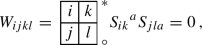  (5.19)

  are equivalent to the integrability condition (5.13).

• (iii) With (5.18), Eq. (5.9) becomes

  $$\begin{aligned} 3\,(n-2)\,\left( \mathring{\textsf{P}}_{ij} - \frac{1}{2}\,\tau _{ij} \right) = \left( (n-2)(S_{ija}\bar{t}^a+\bar{t}_i\bar{t}_j) - {S_{i}}^{ab}S_{jab} \right) _\circ \ . \end{aligned}$$

  (5.20)

Proof

For the first part simply resubstitute (5.18) into (5.10). The proof of part (ii), namely of Equation (5.19), is analogous to that of Theorem 5.9 in [KSV23]. Finally, for part (iii), resubstitute (5.18) into Eq. (5.9). We obtain (5.20). $\quad \square$

As an immediate consequence of (5.18) and (5.19), we obtain the following obstruction on the geometry underlying an abundant system.

Corollary 5.12

Abundant conformally superintegrable systems can only exist on conformally flat manifolds.

Proof

It follows immediately from (5.19) that an abundant conformally superintegrable system can only exist on a Weyl flat manifold. Therefore, for dimension $n\geqslant 4$, they can exist only on conformally flat manifolds. In dimension 2, any metric is conformally flat. We are therefore left with the case $n=3$. Using standard scale, i.e. ${\bar{t}}=0$, Eq. (5.18c) yields that

$$\begin{aligned} {S_{i}}^{ab} S_{jab} - \frac{3}{20}\,S^{abc}S_{abc}\,g_{ij} \end{aligned}$$

is a Codazzi tensor. The claim then follows from the Weyl-Schouten Theorem. $\quad \square$

6 Equivalence Classes of Abundant Superintegrable Systems

So far, we have considered conformally superintegrable systems whose underlying geometry is a (pseudo-) Riemannian manifold. We now turn towards conformal equivalence classes, i.e. towards c-superintegrable systems on conformal manifolds. For such systems, $S_{ijk}$ is the conformally invariant structure tensor. According to (5.20), the secondary structure tensor $\tau _{ij}$ is determined by $T_{ijk}$ and the Ricci curvature. Table 2 contrasts the setting of properly and conformally superintegrable systems as opposed to c-superintegrable systems.

Table 2 Synopsis of the main objects in proper, conformal and c-superintegrability

6.1 Obstructions to the integrability of the non-linear prolongation

Consider the non-linear prolongation (5.18) of PDEs for ${\bar{t}}$ and $S_{ijk}$. We now investigate the integrability conditions for this system. The prolongation Eq. (5.18) are non-linear in the components of $S_{ijk}$ and ${\bar{t}}_i$. Therefore the Ricci conditions,

(6.1a)

(6.1b)

are necessary, but need not be sufficient for the integrability of (5.18). Sufficiency is guaranteed if not only the Ricci condition, but also all of its differential consequences are satisfied in a given point $x_0$ [Gol67]. We find that the integrability conditions, of which a priori there can be infinitely many, reduce to a single algebraic equation of the form (1.3).

Theorem 6.1

• (i) If Eq. (5.19) holds, then the integrability conditions (6.1) of (5.18) are satisfied.

• (ii) Let M be a conformally flat, pseudo-Riemannian manifold of dimension $n\geqslant 3$ and let $x_0\in M$ be a point on this manifold. Then any solution $\Psi _{ijk}=S_{ijk}(x_0)$ of (1.3) together with the arbitrary initial values ${\bar{t}}(x_0)$ and $\nabla \bar{t}(x_0)$ can be extended, in a neighborhood of $x_0$, to solutions $S_{ijk}(x)$ and ${\bar{t}}(x)$ of the non-linear prolongation (5.18).

Proof

• (i) Since the integrability condition cannot depend on ${\bar{t}}$, we may w.l.o.g. perform a conformal transformation such that the transformed system is in standard scale, ${\bar{t}}=0$. As a result, (5.18a) and (5.18b) determine the Ricci curvature tensor in this scale. We shall comment on this after finishing the proof. First, let us investigate the integrability condition for (5.18c), which by virtue of the aforementioned transformation has turned into

  

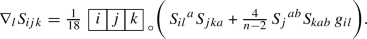  (6.2)

  Using (5.18a), (5.18b) and Weyl-flatness (5.19), we replace the Riemann curvature in (6.1a) by a quadratic expression in S. Due to (5.19) in combination with the non-linear prolongation (5.18) and (5.20), Eq. (6.1a) is equivalent to the conformally invariant condition

  

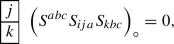
  which is confirmed to be an algebraic consequence of (5.19) by way of contracting (5.19) with S. We have therefore established (5.19) as the only first order integrability condition of (5.18c). By an analogous computation we then confirm that all Ricci identities of (5.18) are satisfied if (5.19) holds. As explained earlier, however, the first order integrability conditions (6.1) need not be sufficient for the integrability of (5.18). We now proceed to show their sufficiency.

• (ii) In order to find sufficient, pointwise integrability criteria, higher order integrability conditions have to be taken into account. Concretely, all differential consequences of (5.19) need to be satisfied in a fixed point $x_0$ in order to allow us to extend $S_{ijk}$ and ${\bar{t}}$ such that the extensions satisfy (5.18) in a neighborhood of $x_0$. Taking a covariant derivative of (5.19) and replacing derivatives of $S_{ijk}$ by (6.2), we find an algebraic condition on $S_{ijk}$. Using (5.19) again, it is verified that this second order condition is an algebraic consequence of the first order one, i.e. (5.19). $\quad \square$

If instead of a pseudo-Riemannian manifold we consider a conformal manifold, we obtain the following statement.

Corollary 6.2

Let $(M,{\textbf{g}})$ be a flat conformal manifold of dimension $n\geqslant 3$. A solution of (1.3) can be extended to ${S_{{ij}}}^k(x)$ in a neighborhood of a point $x_0\in M$, such that for $g=\Omega ^{-2}{\textbf{g}}$ (where $\Omega >0$ is a scalar function) the totally symmetric and trace-free tensor field $S_{ijk}(x)$ satisfies (6.2).

Proof

Note that (1.3) is an invariant condition. The statement follows from statement (ii) in the theorem, making use of the fact that there exists a flat conformal scale choice, which removes the curvature from the non-linear prolongation system (5.18). If (1.3) holds in $x_0\in M$ for this case, the system is integrable in a neighborhood of $x_0$. Note that the specific scale choice is technical and irrelevant for the statement. $\quad \square$

Corollary 6.3

In dimension $n=3$, (5.18) can be integrated for any $S_{ijk}(x_0)$.

Proof

Note that (5.19) has Weyl symmetry and thus vanishes trivially in dimension $n=3$. $\quad \square$

6.2 The conformal factors between standard scale, proper scale and flat scale

In the standard scale ${\bar{t}}=0$, Equations (5.18a) and (5.18b) become algebraic conditions on the curvature tensor. In contrast, if a flat scale exists, exactly the curvature terms disappear. In an arbitrary scale choice we have the following formula for the curvature, in terms of the conformally invariant tensor $S_{ijk}$ and the conformal scale function $\sigma$.

Proposition 6.4

The Ricci tensor satisfies

$$\begin{aligned} {R}_{ij}= -\frac{1}{9}\,\left( {S_{i}}^{ab}S_{jab}+\frac{n}{3(n+2)}\,g_{ij}S^{abc}S_{abc}\right) + (n-2)\,\left( \frac{\mathring{\nabla }^2_{ij}\sigma }{\sigma } -\frac{4(n-1)}{n(n-2)^2}\, \frac{\Delta \sigma ^{\frac{n-2}{2}}}{\sigma ^{\frac{n-2}{2}}}\,g_{ij} \right) \end{aligned}$$

(6.3)

where $\sigma =\exp (-\frac{1}{3}{\bar{t}}\,)$ is the conformal scaling from Definition 4.7.

Proof

Solve (5.18a) and (5.18b) for the Ricci tensor. $\quad \square$

On the right hand side of (6.3), the first term is invariant (up to a conformal factor), while the second term vanishes in standard scale. In a flat scale, $R_{ijkl}=0$, and the left hand side vanishes. The function ${\bar{t}}=\rho$ arising from the primary structure tensor measures ‘how far’ the flat scale is from the standard scale. According to (4.12), the conformal scale factor between the two scales is

$$\begin{aligned} \theta :=e^{-\frac{1}{3}\rho } \end{aligned}$$

(6.4)

(note that we transform from the scale defined by $h_{ij}$ back to the standard scale with metric ${\mathfrak {g}}_{ij})$. From (6.3) we see that the flat conformal scales $\theta$ are determined by $S_{ijk}$. The following lemma makes this explicit.

Lemma 6.5

For any conformal class of abundant superintegrable systems there are functions $\theta >0$ satisfying

$$\begin{aligned} \mathring{\nabla }^2_{ij}\theta&= -\frac{\left( {S_{i}}^{ab}S_{jab} \right) _\circ }{9(n-2)}\,\theta \end{aligned}$$

(6.5a)

$$\begin{aligned} \Delta \theta ^{1-\frac{n}{2}}&= \frac{(n-2)(3n+2)}{36(n-1)(n+2)}\,S^{abc}S_{abc}\, \theta ^{1-\frac{n}{2}}\,. \end{aligned}$$

(6.5b)

where $\mathring{\nabla }^2$ is the flat, trace-free Hessian and $\Delta$ the flat Laplace operator, and where $S_{ijk}$ is the conformal structure tensor in the flat scale.

Proof

Let the function ${\bar{t}}=\rho$ be the trace of the structure tensor after a conformal transformation to a flat scale. Then a conformal transformation with $\Upsilon =-\frac{\nabla \rho }{\rho }$ takes us back to the standard scale. Rewriting (5.18a) and (5.18b) in terms of $\theta$, and decomposition of the result into its trace-free and trace parts, confirms the claim. $\quad \square$

Solutions $\theta$ are not unique. Indeed, a positive constant scalar multiple of $\theta$ is again a solution, and, in general, more solutions can exist. For instance, in Table 3 the systems III and V are both in flat scale, and they are conformally equivalent, see [Cap14]. Two different solutions $\theta$ represent two different flat conformally superintegrable systems within the same conformal class. They share the same ${{\mathring{T}}_{ij}}{}^{k}={S_{ij}}^k$ but the traces of $T_{ijk}$ will be different unless the ${\bar{t}}$ differ only by an additive constant. In order to understand the space of solutions $\theta$ better, let us study (6.5a) further, ignoring the additional constraint (6.5b) for a moment. We find:

Lemma 6.6

Equation (6.5a) has the linear prolongation

$$\begin{aligned} \nabla ^2_{ij}\theta&= -\frac{({S_{i}}^{ab}S_{jab})_\circ }{9(n-2)}\,\theta +\frac{1}{n}\,g_{ij}\,\Delta \theta \end{aligned}$$

(6.6a)

$$\begin{aligned} (\Delta \theta )_{,k}&= \frac{n}{9(n-2)}\,S^{abc}S_{kab}\,\theta _{,c} +\frac{3n+2}{27(n-1)(n-2)}\, {S_{k}}^{ab}{S_{a}}^{cd}S_{bcd}\,\theta \end{aligned}$$

(6.6b)

where $\nabla ^2$ is the flat Hessian and $\Delta$ the flat Laplace operator, and where $S_{ijk}$ is the conformal structure tensor in the flat scale. The integrability conditions for (6.6) are equivalent to (5.19).

Proof

Equations (6.6) are obtained in formal analogy to (4.1), where formally $T\equiv 0$. Its integrability conditions are satisfied due to (5.19), as (6.6a) is a special case of (5.18a).

$\square$

Equations (6.6) are a linear prolongation system for $\theta$ whose coefficients are determined by $S_{ijk}$. Its solutions $\theta$ lie in an (at most) $(n+2)$-dimensional linear space, determined by the values of $\Delta \theta ,\nabla \theta$ and $\theta$ in a fixed point. The additional constraint (6.5b) defines a quadric in this space.

6.3 Classifying the conformal classes of conformally superintegrable systems

In the previous section we have found algebraic integrability conditions whose form is the same for any conformally superintegrable system within a class (in the next section we reformulate them as equivariant conditions). As initial data we need to specify $\Psi _{ijk}=S_{ijk}(x_0)$. For a conformally flat geometry we may choose a flat metric, which facilitates determining a solution for $S_{ijk}$. In order to reconstruct an abundant conformally superintegrable system from the initial data $\Psi _{ijk}=S_{ijk}(x_0)$, we recall that an abundant superintegrable system requires a conformally flat metric $g=\phi ^2\,h$ where h is the flat metric. Then we can use the following procedure.

• (i) Let $\Psi _{ijk}=S_{ijk}(x_0)$ be the initial data given in a point $x_0$. Assume that $\Psi _{ijk}$ solves the algebraic condition (1.3). The $\Psi _{ijk}$ do not depend on $\phi$, and if $\Psi _{ijk}$ are solutions then so are $k\Psi _{ijk}$ for $k\ne 0$.

• (ii) We extend the initial data $\Psi _{ijk}$ to a solution in a neighborhood of $x_0$ such that the non-linear prolongation (5.18) holds. This is possible by virtue of Corollary 6.2. For a concrete computation we should choose some conformal scale, and the flat scale is a reasonable choice. We then need to specify the initial data $\nabla \rho (x_0)$ and $\rho (x_0)$ in addition to $\Psi _{ijk}$.

• (iii) This yields $T_{ijk}$ up to a conformal transformation. Integrating the Wilczynski Eq. (3.14) for V in the specific scale given by ${\bar{t}}=\rho$, and computing ${\textbf{v}}=e^{\frac{2\rho }{3}}V$, we find the conformally invariant potential as an $(n+2)$-parameter family of densities of weight $-2$. This is the space ${\mathcal {V}}^\text {max}$. The space ${\mathcal {C}}^\text {max}$ of conformal Killing tensors is similarly obtained by integration of (5.1).

Since all integrability conditions are satisfied generically, we find at least $\tfrac{1}{2}\,n(n+1)$ many linearly independent conformal integrals. We address their functional independence below in Lemma 6.7.

The procedure just outlined allows one to reconstruct an abundant c-superintegrable system from the given initial data and the knowledge of the underlying conformal metric up to the choice of the potential from ${\mathcal {V}}^\text {max}$. We recall Assumption 3.6, but remark that with Lemma 6.7 below, we are able to restrict the space ${\mathcal {C}}^\text {max}$ in order to obtain $2n-1$ functionally independent conformal integrals. Let us reinterpret the aforesaid in the light of classifying c-superintegrable systems. In [KSV23, Theorem 6.4] it is shown that the classification space for irreducible non-degenerate superintegrable systems on a (pseudo-) Riemannian manifold M with analytic metric is a quasi-projective subvariety ${\mathcal {U}}\subset G_{2n-1}(\mathcal K(M))$ in the Grassmannian of $(2n-1)$-dimensional subspaces in the space ${\mathcal {K}}(M)$ of Killing tensors on M. Since any c-superintegrable system admits at least one system in proper scale, it follows that the classification space of irreducible non-degenerate c-superintegrable systems with analytic metric is the quotient $\tilde{{\mathcal {U}}}={\mathcal {U}}/\textrm{Conf}(M)$. For non-degenerate irreducible conformally superintegrable systems on analytic metrics, the classification space is a fibre bundle over $\tilde{{\mathcal {U}}}$.

The following lemma was proven for properly superintegrable systems in reference [KSV23]. We adapt it for conformal systems.

Lemma 6.7

Let $C^{(\alpha )}$ be $2n-2$ linearly independent, trace-free conformal Killing tensors satisfying the integrability conditions (5.15) for (5.1), and (4.2) for (4.1). Then, in the linear space ${\mathcal {V}}^\text {max}$ of solutions V to Eq. (4.1), those V that give rise to functionally dependent integrals are confined to an affine subspace of ${\mathcal {V}}$ with non-empty complement.

Proof

Suppose the integrals (3.4) were functionally dependent. Then there is a function $\varphi :{\mathbb {R}}^{2n-2}\rightarrow {\mathbb {R}}$, non-zero in an open subset of its domain, such that

$$\begin{aligned} \varphi (F^{(1)},\ldots ,F^{(2n-2)})=0 \end{aligned}$$

(6.7)

This implies the infinitesimal condition

$$\begin{aligned} \sum _{\alpha =1}^{2n-2} \lambda _{(\alpha )} dF^{(\alpha )} =0, \end{aligned}$$

(6.8)

where

$$\begin{aligned} \lambda _{(\alpha )}&=\frac{\partial \varphi }{\partial F^{(\alpha )}}(F^{(\alpha )})\,,&dF^{(\alpha )}&=\frac{\partial F^{(\alpha )}}{\partial x^k}dx^k +\frac{\partial F^{(\alpha )}}{\partial p^k}dp^k\,. \end{aligned}$$

By a direct computation we find

$$\begin{aligned} \frac{\partial F^{(\alpha )}}{\partial x^k}&= C^{(\alpha )}_{ij,k}p^ip^j+V^{(\alpha )}_{,k}\,,&\frac{\partial F^{(\alpha )}}{\partial p^k}&= 2C^{(\alpha )}_{jk}p^j. \end{aligned}$$

Separating the components of (6.8) and substituting (3.7), we conclude

$$\begin{aligned} \sum _\alpha \lambda _{(\alpha )}\left( C^{(\alpha )}_{ij,k}p^ip^j +C^{(\alpha )}_{jk}V^{,j} +\omega ^{(\alpha )}_kV \right)&=0 \end{aligned}$$

(6.9a)

$$\begin{aligned} \sum _\alpha \lambda _{(\alpha )} C^{(\alpha )}_{jk}p^j&=0. \end{aligned}$$

(6.9b)

Invoking (5.1), we obtain

$$\begin{aligned} C^{(\alpha )}_{ij,k}p^ip^j&=\frac{2}{3} \left( {{T^a}_{ij}}C^{(\alpha )}_{ka} - {{T^a}_{kj}}C^{(\alpha )}_{ia} \right) p^ip^j -\frac{2}{3n}\,\left( {{T_k}^{ab}}C_{ab}^{(\alpha )} -t^aC_{ak}^{(\alpha )} \right) \,p^cp_c\,. \end{aligned}$$

Multiplying with $\lambda _{(\alpha )}$ and summing over $\alpha$, we find, using (6.9b) and the decomposition (4.7),

$$\begin{aligned} \sum _\alpha \lambda _{(\alpha )} C^{(\alpha )}_{ij,k}p^ip^j&=\frac{2}{3} \sum _\alpha \lambda _{(\alpha )} \left( {{S^a}_{ij}}C^{(\alpha )}_{ka} -\frac{1}{n}\,t^ag_{ij}C^{(\alpha )}_{ka} -\frac{1}{n}\,{{S_k}^{ab}}C_{ab}^{(\alpha )}g_{ij} \right) \,p^ip^j\,. \end{aligned}$$

Substituting this back into (6.9a), invoking (3.2), and using again the decomposition (4.7), we conclude

$$\begin{aligned} C_{ab}\eta ^{kab} = 0\,, \end{aligned}$$

(6.10)

where we use the abbreviations

$$\begin{aligned} C_{ab}:=\sum _\alpha \lambda _{(\alpha )} C^{(\alpha )}_{ab} \end{aligned}$$

and

$$\begin{aligned} \eta ^{kab}= & {} g^{ka} \left( {{S^b}_{ij}}p^ip^j -\frac{1}{n}t^bp^cp_c +\frac{3}{2}\,V^{,b} -\frac{1}{n}\,\frac{(n+1)(n-2)}{(n-1)(n+2)}t^b\,V \right) \\{} & {} +\frac{1}{n}\,S^{kab}\,(V-p^cp_c). \end{aligned}$$

Note that $C(x_0)\not =0$. Indeed, otherwise the $C^{(\alpha )}_{ab}(x_0)$ would be linearly dependent,

$$\begin{aligned} \sum _{\alpha }k_{(\alpha )}C^{(\alpha )}_{ab}(x_0)=0, \qquad k_{(\alpha )}=\lambda _{(\alpha )}(x_0). \end{aligned}$$

Because of (5.1) the derivatives of $C^{(\alpha )}_{ab}$ are linearly dependent at $x_0$, with the same constants $k_{(\alpha )}$. Iterated application of (5.1) to higher derivatives shows that the same is true for all higher derivatives. It readily follows that $\sum _\alpha k_{(\alpha )}C^{(\alpha )}=0$ everywhere, which contradicts the linear independence of the conformal Killing tensors $C^{(\alpha )}$.

Now, for $x_0\in M$, consider the mapping $\Xi :T^{\otimes 3}_{x_0}M\rightarrow T_{x_0}M$, given by contracting with $C_{ab}$,

$$\begin{aligned} \Xi (\eta ^{kab}) = C_{ab}\eta ^{kab}. \end{aligned}$$

By virtue of Eq. (6.10), we conclude that for any potential $V\in {\mathcal {V}}^\text {max}$

$$\begin{aligned} \eta ^{kab}(x_0)\,\,\in \,\ker \Xi . \end{aligned}$$

Using the linearity of the kernel, we conclude further that

$$\begin{aligned} \left[ \frac{3}{2}\,g^{kb}V^{,a} +\frac{1}{n}\,\left( S^{kab} -\frac{(n+1)(n-2)}{(n-1)(n+2)}g^{kb}t^a \right) \,V \right] _{x_0} \,\,\in \,\ker \Xi . \end{aligned}$$

Choosing $V(x_0)=0$, we obtain that

$$\begin{aligned} {{C_k}}^aV_{,a}(x_0)=0 \end{aligned}$$

for any choice of $V_{,a}(x_0)$, contradicting that $C(x_0)\not =0$. $\quad \square$

Theorem 6.8

Abundant conformally superintegrable Hamiltonians with their $(n+2)$-parameter family of potentials, and identified under conformal transformations, are classified by (1.3).

Proof

An abundant conformally superintegrable Hamiltonian with its $(n+2)$-dimensional space ${\mathcal {V}}^\text {max}$ of all compatible potentials, can be recovered from $S_{ijk}$ up to a conformal transformation of superintegrable systems and every abundant system satisfies (1.3).

$\square$

6.4 Invariant formulation of the non-linear prolongation equations

In this section we express the non-linear prolongation equations (5.18) in a conformally invariant way.

Proposition 6.9

• (i) Equation (5.18a) is equivalent to

  $$\begin{aligned} \mathring{{\mathbb {H}}}_{ij}\sigma = -\frac{1}{9(n-2)}\,\left( {{S_i}^{ab}}S_{jab} \right) _\circ \,\sigma \,, \end{aligned}$$

  (6.11)

  where $\sigma =e^{-\frac{1}{3}\,{\bar{t}}}$ and where $\mathring{{\mathbb {H}}}$ is the conformally invariant trace-free Hessian, defined by

  $$\begin{aligned} \mathring{{\mathbb {H}}}_{ij} = \left( \nabla ^2_{ij}-\textsf{P}_{ij}\right) _\circ . \end{aligned}$$

• (ii) Equation (5.18b) is equivalent to

  $$\begin{aligned} {\mathbb {L}}\sigma ^{1-\frac{n}{2}} = -\frac{2}{9}\,\frac{3n+2}{n+2}\,S^{abc}S_{abc}\,\sigma ^{1-\frac{n}{2}}\,, \end{aligned}$$

  (6.12)

  where ${\mathbb {L}}$ denotes the conformal Laplacian,

  $$\begin{aligned} {\mathbb {L}} = -4\,\frac{n-1}{n-2}\,\Delta + R. \end{aligned}$$

• (iii) Equation (5.18c) is equivalent to

  

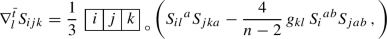  (6.13)

  where $\nabla ^{{\bar{t}}}$ is the conformally equivariant Weyl connection [Wey18] defined by

  $$\begin{aligned} \nabla ^{{\bar{t}}}_i\alpha _j = \nabla _i\alpha _j - \frac{w+1}{3}\,\bar{t}_i\alpha _j - \frac{1}{3}\,{\bar{t}}_j\alpha _i + \frac{1}{3}\,\bar{t}^a\alpha _ag_{ij}\,, \end{aligned}$$

  (6.14)

  for $\alpha _j$ of conformal weight $w=-\frac{2}{3}$, i.e. $\alpha _j\mapsto \Omega ^w\alpha _j$ under conformal transformations.

Proof

Parts (i) and (ii) are straightforward. For part (iii), apply (6.14) to $S_{ijk}$,

A direct computation indeed confirms that $\nabla ^{{\bar{t}}}$ is invariant under conformal changes up to multiplication by a factor: The replacement rules are $g\rightarrow \Omega ^2\,g$ and ${\bar{t}}\rightarrow \bar{t}-3\ln |\Omega |$, as well as, respectively, $S_{ijk}\rightarrow \Omega ^2 S_{ijk}$ or $\alpha _i\rightarrow \Omega ^w\alpha _i$ with $w=-\frac{2}{3}$. $\quad \square$

Two remarks are in place with regard to the above proposition. First, note that the conformal weights required for the trace-free conformal Hessian and the conformal Laplacian are different, leading to different powers of the conformal scale function. The second remark concerns the conformal invariance of the operators. Note that, under conformal transformations with rescale function $\Omega$, we have

$$\begin{aligned} \sigma ^{1-\frac{n}{2}}\rightarrow \Omega ^{1-\tfrac{n}{2}}\,\sigma ^{1-\frac{n}{2}}, \end{aligned}$$

and the conformal invariance of ${\mathbb {L}}$ means

$$\begin{aligned} {\mathbb {L}}\circ \Omega ^{1-\frac{n}{2}} = \Omega ^{-1-\frac{n}{2}}\circ {\mathbb {L}}, \end{aligned}$$

which is consistent as $S^{abc}S_{abc}\rightarrow \Omega ^{-2}S^{abc}S_{abc}$. Note that in the standard scale, i.e. for $\bar{t}=0$ resp. $\sigma =1$, Eq. (6.12) is an expression for the scalar curvature in terms of $S_{ijk}$, and (6.11) for the Schouten tensor.

Remark 6.10

To determine whether the non-linear system (5.18) is integrable, it is sufficient to know the invariants in (6.11), (6.12) and (6.13) as well as those in (6.6), which are constructed algebraically from S.

These invariants are

The last of these invariants has the following geometric interpretation. Due to (5.18a),

$$\begin{aligned} \mathring{{\mathfrak {P}}}_{ij} = \frac{1}{9(n-2)}\,\mathring{\Sigma }_{ij}, \end{aligned}$$

where ${\mathfrak {P}}_{ij}$ denotes the Schouten curvature for the standard scale. Its trace satisfies

$$\begin{aligned} {{{\mathfrak {P}}^a}_{\, a}} = \frac{3n+2}{18(n-1)(n+2)}\,{\Sigma ^a}_a. \end{aligned}$$

The invariant $B_k$ also has a geometric meaning. It is easy to show that

$$\begin{aligned} {{{\mathfrak {P}}^a}_{a,k}} = -\frac{(3n+2)\,B_k}{27(n-2)(n-1)}\,, \end{aligned}$$

(6.15)

and therefore $B_k=0$ characterises the case when the standard scale system has constant scalar curvature. Note that $B_k$ and ${\Sigma ^a}_a$ are not (differentially) independent.

6.5 Properly superintegrable systems on constant curvature manifolds

In the reference [KSV23] abundant properly superintegrable systems are studied. These systems satisfy $\tau _{ij}=0$ due to Lemma 3.15 and thus (5.20) becomes

$$\begin{aligned} \left[ (n-2)(S_{ija}\bar{t}^a+\bar{t}_i\bar{t}_j) - {S_{i}}^{ab}S_{jab} \right] _\circ = 3\,\mathring{R}_{ij}\,. \end{aligned}$$

(6.16)

For a metric of constant sectional curvature, the right hand side of (6.16) vanishes. Moreover, [KSV23] shows that, for constant curvature, (6.16) and (5.18) imply that

$$\begin{aligned} S^{abc}S_{abc} - (n-1)(n+2)\,{\bar{t}}^a {\bar{t}}_a = 9 R\,. \end{aligned}$$

(6.17)

Theorem 6.11

Let g be of constant sectional curvature. If $\tau _{ij}=0$ and (6.17) hold, then

$$\begin{aligned} \Delta \sigma ^{n+2} = -2\,\frac{n+1}{n-1}\,R\,\sigma ^{n+2} \end{aligned}$$

(6.18)

where $\sigma =e^{-\frac{1}{3}\bar{t}}$ as in Definition 4.7.

Proof

If (6.17) holds, then $S^{abc}S_{abc}$ can be eliminated from Eq. (5.18b), yielding

$$\begin{aligned} \Delta \bar{t} = \frac{6(n+1)}{(n-1)(n+2)}\,R +\frac{n+2}{3}\,\bar{t}^{,a}\bar{t}_{,a}\,. \end{aligned}$$

In terms of $\sigma =e^{-\frac{1}{3}\,{\bar{t}}}$, this rewrites as (6.18). $\quad \square$

For constant curvature spaces, Eq. (5.18b) thus becomes a Laplace eigenvalue problem, and a power of the scale function $\sigma$ is an eigenfunction of $\Delta$. For a flat manifold, (6.18) merely implies that $\sigma ^{n+2}$ is harmonic. On the round sphere ${\mathbb {S}}^n\subset {\mathbb {R}}^{n+1}$, we have spherical harmonics with the quantum number $\mu =n+1$ satisfying

$$\begin{aligned} \mu \,(\mu +n-1) := 2\,\frac{n+1}{n-1}\,Rr^2 = 2\,n(n+1)\,, \end{aligned}$$

(6.19)

where the second equality follows from $R=\frac{n(n-1)}{r^2}$ with $r>0$ denoting the radius of the sphere.

A close connection between the Helmholtz-Laplace equations and conformal superintegrability has been found in [KMS16, KKMP11]. Such links also appear in the present paper, although in different context: Earlier we have seen that on conformally flat spaces we find a scalar function $\theta ^{1-\frac{n}{2}}$ satisfying the generalised Helmholtz Eq. (6.5b). Now we have found (6.12), which is a conformally invariant generalised Helmholtz equation. In particular, in the case of proper superintegrability, the $(n+2)$-nd power of the conformal scale function satisfies the generalised Helmholtz Eq. (6.18). It is a proper Helmholtz equation in the case of constant scalar curvature.

We use Eq. (6.18) to study conformally equivalent properly superintegrable systems further.

Proposition 6.12

Assume we are provided with an abundant second order properly superintegrable system on the sphere with the round metric g, which is conformally equivalent to a properly superintegrable system on flat space with the flat metric $h=\Omega ^{-2}g$. Then the conformal factor $\sigma$ on the sphere has to satisfy

$$\begin{aligned} \Omega \,\left( \Delta \Omega -g(d\ln (\sigma ^{n+2}),d\Omega )\right) + \,g(d\Omega ,d\Omega ) = 0\,. \end{aligned}$$

(6.20)

Note that $\Omega$ is the conformal factor mediating between the standard and the spherical scale, while $\sigma$ mediates between the spherical and the flat scale.

Proof

Due to (6.18), a properly superintegrable system on flat space must satisfy the condition $\Delta _\text {flat}(\Omega ^{-(n+2)}\sigma ^{n+2})=0$. A direct computation using (6.18) then shows

$$\begin{aligned} \Delta _\text {flat}(\Omega ^{-(n+2)}\sigma ^{n+2}) = (3n+2)\,\sigma ^{n+2}\Omega ^{-(n+6)}\,\bigg [ \Omega \Delta \Omega + \Omega ^{,a}\Omega _{,a} - \Omega \Omega ^{,a}\,(\ln \sigma ^{n+2})_{,a} \bigg ]\,, \end{aligned}$$

taking into account that

$$\begin{aligned} R = -2\frac{n-1}{\Omega ^2}\,\left( \Omega \Delta \Omega -\frac{n}{2}\,\Omega ^{,a}\Omega _{,a} \right) . \end{aligned}$$

due to (3.24). $\quad \square$

The following example generalises a result shown in [KKM06], which addresses the specific case of dimension 3, see also [Cap14]. The proof presented here is a relatively simple exercise, while with traditional methods the claim, if at all, cannot be obtained for arbitrary dimension in a straightforward fashion.

Example 6.13

(Generic system on the n-sphere) Consider the generic system on the n-sphere, with $n\geqslant 3$, introduced for dimension 3 in Example 4.14. In arbitrary dimension we have the metric

$$\begin{aligned} g = \sum _{m=1}^{n} \left( \prod _{k=2}^{m}\sin ^2(\phi _{k-1})\right) d\phi _m^2 \end{aligned}$$

with angular coordinates $\phi _1,\dots ,\phi _n$. The superintegrable potential defining the generic system is

$$\begin{aligned} V = a_0 + \sum _{m=1}^{n} \left( \frac{a_m}{ \cos ^2(\phi _m) \prod _{k=2}^{m} \sin ^2(\phi _{k-1}) } \right) + \frac{a_{n+1}}{\prod _{k=1}^n \sin ^2(\phi _k)} \end{aligned}$$

For this system, $\sigma ^{n+2}$ satisfies the Laplace eigen-equation with quantum number $n+1$,

$$\begin{aligned} \Delta \sigma ^{n+2} = -2n(n+1)\sigma ^{n+2}. \end{aligned}$$

Solutions of this equation span a vector space of dimension $(n+2)^2$ whose basis is given by hyperspherical harmonics.

Concretely, for the generic system, we have

$$\begin{aligned} \sigma ^{n+2} = \prod _{k=1}^n \cos (\phi _k)\sin ^{n-k+1}(\phi _k), \end{aligned}$$

which does not satisfy (6.20).

We have thus proven the following.

Proposition 6.14

The generic system on the n-sphere is not conformally equivalent to a properly superintegrable system on flat space.

We remark that the generic system on the n-sphere can be transformed into a proper superintegrable systems on flat space using Bôcher transformations or orbit degenerations [Cap14]. Opposed to conformal transformations, however, these are not equivalence relations on conformally superintegrable systems.

Proposition 6.15

A non-degenerate properly superintegrable system on the n-sphere cannot be conformally equivalent to the harmonic oscillator.

Proof

The harmonic oscillator has a vanishing structure tensor, $T_{ijk}=0$. Therefore any system conformally equivalent to the harmonic oscillator must satisfy $S_{ijk}=0$. Being proper, due to (6.11), (6.12) and (6.18), the system on the sphere satisfies

$$\begin{aligned} \mathring{\nabla }^2_{ij}\sigma = 0,\quad \Delta \sigma ^{1-\frac{n}{2}} = 0,\quad \Delta \sigma ^{n+2} = -2\,\frac{n+1}{n-1}\,R\sigma ^{n+2}\ne 0, \end{aligned}$$

where $\mathring{\nabla }^2$ and $\Delta$ are the trace-free Hessian and the Laplace-Beltrami operator on the sphere of constant scalar curvature $R\ne 0$. This system does not admit a solution. $\square$

Definition 6.16

We say that a c-superintegrable system is basic if it contains a member system that is an abundant properly superintegrable system on a manifold of constant curvature.

In reference [KSV23], it is proven that the structure tensor of an abundant second order properly superintegrable system on a constant curvature manifold of dimension $n\geqslant 3$ satisfies

(6.21)

where B is a scalar function, called its structure function. Obviously, the structure function is not unique, but according to [KSV23] it is determined up to addition of a solution $\delta B$ of

(6.22a)

(6.22b)

The next proposition allows one to extend structure functions to all basic c-superintegrable systems.

Proposition 6.17

Consider two manifolds of constant curvature and with properly superintegrable systems that are conformally equivalent. Denote their metrics by g and ${{\tilde{g}}}=\Omega ^2\,g$. Assume the superintegrable systems with underlying metric g has the structure function B. Then the structure function ${{\tilde{B}}}$ for the system of ${{\tilde{g}}}$ can be chosen such that

$$\begin{aligned} {{\tilde{B}}} = \Omega ^2 B\,. \end{aligned}$$

(6.23)

Proof

On a manifold with Hamiltonian $H=g^{ij}p_ip_j+V$, we infer from [KSV23] the following formula for $B_{ijk}$ in an abundant constant-curvature system,

where

$$\begin{aligned} C = \frac{n-2}{n+2}\,\Delta B + \frac{2(n+1)}{n(n-1)}\,RB - (n-2){\bar{t}} \end{aligned}$$

(6.24)

and

up to an irrelevant constant. By virtue of (3.19), we know the transformation rules

$$\begin{aligned} S_{ijk} \mapsto {\tilde{S}}_{ijk}=\Omega ^2S_{ijk}\qquad \text {and}\qquad {\bar{t}}_{,i} \mapsto {\bar{t}}_{,i} -3\Omega ^{-1}\Omega _{,i}, \end{aligned}$$

and therefore that of $B_{ijk}$,

$$\begin{aligned} {{\tilde{B}}}_{ijk} = \Omega ^2 \left( B_{ijk} + \text { trace terms} \right) \,. \end{aligned}$$

(6.25)

Secondly, we also know by construction that , where on the right hand side we recall that comma denotes the covariant derivative. An analogous equation holds for ${{\tilde{S}}}_{ijk}$ with a function ${{\tilde{B}}}$. Now, let us denote by $\nabla$ and ${\tilde{\nabla }}$ the Levi-Civita connections of g and ${{\tilde{g}}}$, respectively. Then, for the third derivatives,

(6.26)

because of the invariance of $S_{ijk}$. A straightforward computation verifies that ${{\tilde{B}}}=\Omega ^2B$ satisfies (6.26). We have therefore confirmed that $\bar{{\tilde{t}}}={\bar{t}}-3\ln |\Omega |$ and ${{\tilde{B}}}=\Omega ^2B$ yield the correct structure tensors ${{\tilde{S}}}_{ijk}$ and $\bar{{\tilde{t}}}_{,i}$ for the conformally transformed manifold with Hamiltonian ${{\tilde{H}}}=\Omega ^{-2}H$. The claim follows since structure functions are unique up to solutions of (6.22). $\quad \square$

In [KSV23] the structure function B is defined for abundant properly superintegrable systems on constant curvature spaces only. We can now define it for any basic c-superintegrable system.

Corollary 6.18

Abundant second order properly superintegrable systems on constant curvature spaces in dimension $n\geqslant 3$ are Stäckel equivalent if and only if their conformal densities ${\textbf{b}}\in {\mathcal {E}}[-2]$,

$$\begin{aligned} {\textbf{b}} = B\,\det (g)^{\frac{1}{n}}\,, \end{aligned}$$

coincide up to a gauge transformation given by a solution of (6.22).

7 Application to Dimension Three

In the present section, we apply our framework to the 3-dimensional case. Non-degenerate second order conformally superintegrable systems in dimension 3 are classified in [KKM06, Cap14]. Also, it is known that all these systems are abundant [KKM05b]. In [KKM06] it has been established that any non-degenerate second order conformally superintegrable system is Stäckel equivalent to a non-degenerate second order abundant and proper system on a constant curvature geometry. We shall therefore restrict to the study of abundant systems for constant curvature metrics. All non-degenerate 3-dimensional systems are equivalent to these. Recall that in dimension 3, the non-linear condition (5.19) is void. Consequently, no further restriction exists on the tensor $S_{ijk}$. Hence any trace-free symmetric initial conditions $\Psi _{ijk}=S_{ijk}(x_0)$ in a point $x_0\in M$ can be integrated for a structure tensor $S_{ijk}$ of an abundant second order conformally superintegrable system, c.f. Corollary 6.3. Therefore the set of conformal equivalence classes of such systems is parametrised by the seven dimensional space of trace-free symmetric 3-tensors $\Psi _{ijk}$ or, equivalently, harmonic ternary cubics $\Psi (\textbf{p})=\Psi _{ijk}{p}^i{p}^j{p}^k$. This parametrisation is equivariant with respect to the stabiliser subgroup of the point $x_0$ in the conformal group, which is isomorphic to $\textrm{SO}(3)$.

Table 3 The properly superintegrable systems in dimension 3 on flat space. The Systems III and V are conformally equivalent

We comment that this agrees with the references [KKMP11, CK14, Cap14]. In [KKMP11] a 10-parameter classification space is mentioned, corresponding to a 10-dimensional representation of $\textrm{SO}(3)$ in [Cap14, CK14]. This 10-dimensional representation decomposes into two irreducible components of dimension 7 and 3, corresponding to $S_{ijk}$ and ${\bar{t}}_{,i}$ in our framework. Note that the 3-dimensional component is restricted in the references, which corresponds to imposing proper superintegrability here. The 7-dimensional component is realised as the space of binary sextics and it is shown that no restrictions exist on this component. The relation to our framework is given by a known correspondence between harmonic ternary cubics and binary sextics as follows.

The adjoint action of $\textrm{SL}(2,{\mathbb {C}})$ on its Lie algebra $\textrm{sl}(2,{\mathbb {C}})\cong {\mathbb {C}}^3$ preserves the Killing form. This defines a group morphism $\textrm{SL}(2,\mathbb C)\rightarrow \textrm{SO}(3,{\mathbb {C}})$ with kernel $\{\pm 1\}$ and hence an isomorphism $\textrm{SL}(2,{\mathbb {C}})/\mathbb Z_2\rightarrow \textrm{SO}(3,{\mathbb {C}})$. The standard action of $\textrm{SL}(2,{\mathbb {C}})$ on ${\mathbb {C}}^2$ induces an $\textrm{SL}(2,{\mathbb {C}})$-action on $S^2{\mathbb {C}}^2$ which descends to an $\textrm{SO}(3,{\mathbb {C}})$-action, because the elements $\pm 1$ act trivially. The latter induces an $\textrm{SO}(3,\mathbb C)$-action on $S^3\,S^2{\mathbb {C}}^2$ which descends to $S^6{\mathbb {C}}^2$ under total symmetrisation $S^3S^2{\mathbb {C}}^2\rightarrow S^6{\mathbb {C}}^2$. Together with the isomorphism $S^2{\mathbb {C}}^2\cong {\mathbb {C}}^3$, we obtain a morphism $S^3{\mathbb {C}}^3\rightarrow S^6{\mathbb {C}}^2$ of $\textrm{SO}(3,{\mathbb {C}})$-representations, giving an $\textrm{SO}(3,{\mathbb {C}})$-equivariant morphism from the 10-dimensional space of ternary cubics to the 7-dimensional space of binary sextics. Its restriction to the 7-dimensional space of harmonic ternary cubics is non-trivial and hence an isomorphism by Schur’s lemma. Explicitly, it is given by defining a sextic s from the cubic $\Psi ({\textbf{p}})$ via

$$\begin{aligned} s(z,w)=\Psi (z^2-w^2,2zw,z^2+w^2). \end{aligned}$$

(7.1)

Note that the stabiliser subgroup contains only rotations. The action of translations is not linear and more involved.

Table 3 lists the established normal forms for 3-dimensional non-degenerate systems on flat space, see [KKM06, Cap14]. The functions B and ${\bar{t}}$ are obtained as established in [KSV23], and due to Proposition 6.17 and Eq. (4.10), we may compute the corresponding functions for any 3-dimensional non-degenerate system conformally equivalent to one of the systems in Table 3. If in Table 3, we take the quotient under conformal equivalence for each example, then the systems III and V are identified (use e.g. Corollary 6.18) and we obtain a list of nine abundant c-superintegrable systems. Due to [Cap14] these are all abundant c-superintegrable systems in dimension 3, up to one exception. Indeed, from [KKM05b, KKM06, Cap14] it follows that there is one equivalence class of non-degenerate 3-dimensional superintegrable system that does not admit a representative properly superintegrable system on flat 3-space. This system is the generic system on the 3-sphere from Example 4.14, see also Proposition 6.14. Its conformally equivariant structure tensor $S_{ijk}$ is generated by the structure function (up to gauge freedom)

$$\begin{aligned} B = -\frac{3}{2}\,\sum _k s_k^2\,\ln (s_k)\,. \end{aligned}$$

References

Bertrand, J.M.: Mémoire sur quelques-unes des forms les plus simples qui puissent présenter les intégrales des équations différentielles du mouvement d’un point matériel. J. Math. Pure Appl. II(2), 113–140 (1857)
Bolsinov, A.V., Kozlov, V.V., Fomenko, A.T.: The Maupertuis principle and geodesic flows on the sphere arising from integrable cases in the dynamics of a rigid body. Russian Mathematical Surveys 50(3), 473–501 (1995)
Boyer, C.P., Kalnins, E.G., Miller, W., Jr.: Stäckel-equivalent Integrable Hamiltonian systems. SIAM J. Math. Anal. 17(4), 778–797 (1986)
Błaszak, M., Marciniak, K.: On Reciprocal Equivalence of Stäckel systems, Studies in Applied Mathematics 129 (2012), no. 1, 26–50
Błaszak, M., Marciniak, K.: Classical and Quantum Superintegrability of Stäckel Systems. SIGMA 13, 008 (2017)
Capel, J.J.: Classification of second-order conformally-superintegrable systems, Ph.D. thesis, School of Mathematics and Statistics, University of New South Wales, 6 (2014)
Curry, S., Gover, R.A.: An introduction to conformal geometry and tractor calculus, with a view to applications in general relativity, arXiv:1412.7559 (2015)
Capel, J.J., Kress, J.M.: Invariant classification of second-order conformally flat superintegrable systems. Journal of Physics A: Mathematical and Theoretical 47, 495202 (2014)
Capel, J.J., Kress, J.M., Post, S.: Invariant classification and limits of maximally superintegrable systems in 3D, SIGMA Symmetry Integrability Geom. Methods Appl. 11 (2015), 038, 17
Darboux, G.: Sur un problème de méchanique. Archives Néerlandaises (ii) 6, 371–376 (1901)
de Maupertuis, Pierre Louis Moreau: Essai de Cosmologie (1750)
Gema, M.: Diaz-Toca, Laureano Gonzalez-Vega, and Henri Lombardi, Generalizing Cramer’s rule: Solving uniformly linear systems of equations. SIAM Journal on Matrix Analysis and Applications 27(3), 621–637 (2005)
Fulton, W., Harris, J.: Representation theory: A first course, springer study edition ed., Graduate Texts in Mathematics, no. 129, Springer-Verlag, (2000)
Fulton, W.: Young tableaux: With applications to representation theory and geometry, London Mathematical Society Student Texts, no. 35, Cambridge University Press, (1997)
Gover, R.A., Leistner, T.: Invariant prolongation of the Killing tensor equation, Ann. Mat. Pura Appl. (4) 198 (2019), no. 1, 307–334
Goldschmidt, H.: Integrability criteria for systems of nonlinear partial differential equations. J. Differential Geom. 1(3–4), 269–307 (1967)
Hietarinta, J., Grammaticos, B., Dorizzi, B., Ramani, A.: Coupling-constant metamorphosis and duality between integrable Hamiltonian systems. Phys. Rev. Lett. 53, 1707–1710 (1984)
Jacobi, C.G.J.: C. G. J. Jacobi’s Vorlesungen über Dynamik. Gehalten an der Universität zu Königsberg im Wintersemester 1842-1843 und nach einem von C. W. Borchart ausgearbeiteten Hefte. Hrsg. von A. Clebsch., Berlin, G. Reimer, 2. rev. Ausg., (1884)
Kalnins, E.G., Kress, J. M., Miller, W. Jr., Second order superintegrable systems in conformally flat spaces. II. The classical two-dimensional Stäckel transform, J. Math. Phys. 46 (2005), no. 5, 053510, 15
Kalnins, E.G., Kress, J.M., Miller, W. Jr., Second order superintegrable systems in conformally flat spaces. III. Three-dimensional classical structure theory, J. Math. Phys. 46 (2005), no. 10, 103507, 28
Kalnins, E.G., Kress, J.M., Miller, W. Jr., Second-order superintegrable systems in conformally flat spaces. I. Two-dimensional classical structure theory, Journal of Mathematical Physics 46 (2005), 053509
Kalnins, E.G., Kress, J.M., Miller, W. Jr., Second order superintegrable systems in conformally flat spaces. IV. The classical 3D Stäckel transform and 3D classification theory, Journal of Mathematical Physics 47 (2006), 043514
Kalnins, E.G., Kress, J.M., Miller, W., Jr.: Nondegenerate 2D complex Euclidean superintegrable systems and algebraic varieties. J. Phys. A 40(13), 3399–3411 (2007)
Kalnins, E.G., Kress, J.M., Miller, W. Jr., Nondegenerate three-dimensional complex Euclidean superintegrable systems and algebraic varieties, J. Math. Phys. 48 (2007), no. 11, 113518, 26
Kalnins, E.G., Kress, J.M., Miller, W.: Separation of variables and superintegrability, 2053-2563, IOP Publishing, (2018)
Kalnins, E.G., Kress, J.M., Miller, W., Jr., Post, S.: Structure theory for second order 2D superintegrable systems with 1-parameter potentials. SIGMA 5, 008 (2009)
Kalnins, E.G., Kress, J.M., Miller, W., Post, S.: Laplace-type equations as conformal superintegrable systems, Advances in Applied Mathematics 46 (2011), no. 1, 396 – 416, Special issue in honor of Dennis Stanton
Kalnins, E.G., Kress, J.M., Miller, W., Jr., Winternitz, P.: Superintegrable systems in Darboux spaces. J. Math. Phys. 44(12), 5811–5848 (2003)
Klein, F.: A comparative review of recent researches in geometry. Bulletin of the New York Mathematical Society 2(10), 215–249 (1900)
Kalnins, E.G., Miller, W., Post, S.: Coupling constant metamorphosis and Nth-order symmetries in classical and quantum mechanics, Journal of Physics A: Mathematical and Theoretical 43 (2009), no. 3, 035202
Kalnins, E.G., Miller, W. Jr., Subag, E.: Bôcher contractions of conformally superintegrable Laplace equations, SIGMA Symmetry Integrability Geom. Methods Appl. 12 (2016), Paper No. 038, 31
Kress, J.M.: Equivalence of superintegrable systems in two dimensions. Physics of Atomic Nuclei 70(3), 560–566 (2007)
Kress, J., Schöbel, K.: An algebraic geometric classification of superintegrable systems in the Euclidean plane, Journal of Pure and Applied Algebra (2018)
Kress, J., Schöbel, K., Vollmer, A.: An Algebraic Geometric Foundation for a Classification of Superintegrable Systems in Arbitrary Dimension, J. Geom. Anal. 33 (2023), no. 360
Kulkarni, R.S.: Curvature structures and conformal transformations. Bull. Amer. Math. Soc. 75, 91–94 (1969)
Kulkarni, R.S.: Curvature structures and conformal transformations. J. Differential Geometry 4, 425–451 (1970)
Lagrange, J.-L.: Mécanique analytique (1788)
Peeters, K.: A field-theory motivated approach to symbolic computer algebra, Computer Physics Communications 176 (2006), no. 8, 550–558, arxiv:arXiv:cs/0608005 [cs.SC]
Peeters, K.: Introducing Cadabra: a symbolic computer algebra system for field theory problems, (2007), arXiv:hep-th/0701238
Post, S.: Coupling constant metamorphosis, the Stäckel transform and superintegrability. AIP Conference Proceedings 1323(1), 265–274 (2010)
Sergyeyev, A., Błaszak, M.: Generalized Stäckel transform and reciprocal transformations for finite-dimensional integrable systems, Journal of Physics A: Mathematical and Theoretical 41 (2008), no. 10, 105205
Sharpe, R.W., Chern, S.S.: Differential geometry: Cartan’s generalization of Klein’s Erlangen program. Graduate Texts in Mathematics, Springer, New York (2000)
Tsiganov, A.V.: The Maupertuis principle and canonical transformations of the extended phase space. J. Nonlinear Math. Phys. 8(1), 157–182 (2001)
Valent, G.: Global structure and geodesics for Koenigs superintegrable systems. Regul. Chaotic Dyn. 21(5), 477–509 (2016)
Vollmer, A.: Projectively equivalent 2-dimensional superintegrable systems with projective symmetries, Journal of Physics A: Mathematical and Theoretical 53 (2020), no. 9, 095202
Weir, G.J.: Conformal Killing tensors in reducible spaces. Journal of Mathematical Physics 18(9), 1782–1787 (1977)
Weyl, H.: Reine Infinitesimalgeometrie, Mathematische Zeitschrift 2 (1918), 384–411 (ger)
Wilczynski, E.J.: Projective differential geometry of curved surfaces. I, Trans. Amer. Math. Soc. 8 (1907), no. 2, 233–260
Wilczynski, E.J.: Projective differential geometry of curved surfaces. IV, Trans. Amer. Math. Soc. 10 (1909), no. 2, 176–200
Wolf, T.: Structural equations for Killing tensors of arbitrary rank. Computer Physics Communications 115(2–3), 316–329 (1998)
Acknowledgements
We would like to thank Rod Gover for discussions and insightful input from the viewpoint of parabolic and conformal geometry, and for travel support via the Royal Society of New Zealand from Marsden Grant 16-UOA-051. We are grateful towards Benjamin McMillan, Thomas Leistner and Paul-Andy Nagy for helpful comments and discussions from the angle of conformal geometry and representation theory. We thank Vladimir Matveev for comments on integrability, analyticity and projective geometry. We are indepted to Joshua Capel for his insights into superintegrable systems in dimension 3 and the classification of their Stäckel classes. We also thank Jeremy Nugent for discussions. We thank the authors and contributors of the computer algebra system cadabra2 [Pee06, Pee07], which we have used to find, prove and simplify some of the most important results in this work, for providing, maintaining and extending their software and distributing it under a free license. We acknowledge support from ARC Discovery Project grant DP190102360. The project was funded by Deutsche Forschungsgemeinschaft (DFG, German Research Foundation), Project number 353063958; AV also acknowledges support through the project PRIN 2017 “Real and Complex Manifolds: Topology, Geometry and holomorphic dynamics”, and the MIUR grant “Dipartimenti di Eccellenza 2018–2022 (E11G18000350001)”.
Funding
Open Access funding enabled and organized by CAUL and its Member Institutions.
Author information
Authors and Affiliations
Corresponding author
Additional information
Communicated by J.d-Gier.
Publisher's Note
Springer Nature remains neutral with regard to jurisdictional claims in published maps and institutional affiliations.
Rights and permissions
Open Access This article is licensed under a Creative Commons Attribution 4.0 International License, which permits use, sharing, adaptation, distribution and reproduction in any medium or format, as long as you give appropriate credit to the original author(s) and the source, provide a link to the Creative Commons licence, and indicate if changes were made. The images or other third party material in this article are included in the article’s Creative Commons licence, unless indicated otherwise in a credit line to the material. If material is not included in the article’s Creative Commons licence and your intended use is not permitted by statutory regulation or exceeds the permitted use, you will need to obtain permission directly from the copyright holder. To view a copy of this licence, visit http://creativecommons.org/licenses/by/4.0/.
About this article
Cite this article
Kress, J., Schöbel, K. & Vollmer, A. Algebraic Conditions for Conformal Superintegrability in Arbitrary Dimension. Commun. Math. Phys. 405, 92 (2024). https://doi.org/10.1007/s00220-023-04872-w
Received:
Accepted:
Published:
DOI: https://doi.org/10.1007/s00220-023-04872-w