
Abstract
The quantum random energy model (QREM) is a random matrix of Anderson-type which describes effects of a transversal magnetic field on Derrida’s spin glass. The model exhibits a glass phase as well as a classical and a quantum paramagnetic phase. We analyze in detail the low-energy spectrum and establish a localization-delocalization transition for the corresponding eigenvectors of the QREM. Based on a combination of random matrix and operator techniques as well as insights in the random geometry, we derive next-to-leading order asymptotics for the ground-state energy and eigenvectors in all regimes of the parameter space. Based on this, we also deduce the next-to-leading order of the free energy, which turns out to be deterministic and on order one in the system size in all phases of the QREM. As a result, we determine the nature of the fluctuations of the free energy in the spin glass regime.
1 Introduction and Main Results
1.1 Quantum random energy model
In the theory of disordered systems the random energy model (REM) is a simple, yet ubiquitous toy model. It assigns to every N-bit or Ising string \( \pmb {\sigma } = (\sigma _1, \dots , \sigma _N) \in \{ -1, 1\}^N {=}{:}{\mathcal {Q}}_N \) a rescaled Gaussian random variable
with \( \left( \omega (\pmb {\sigma }) \right) \) forming \( 2^N \) canonically realized independent and identically distributed (i.i.d.) random variables with standard normal law \( {\mathbb {P}} \). The Hamming cube \( {\mathcal {Q}}_N \) is rendered a graph by declaring two bit strings connected by an edge if they differ by a single bit flip: introducing the flip operators \( F_j\pmb {\sigma }:= (\sigma _1, \dots , - \sigma _j, \dots , \sigma _N ) \) on components \( j \in \{ 1, \dots , N \} \), the edges of the Hamming cube are formed by all pairs of the form \( ( \pmb {\sigma }, F_j\pmb {\sigma } )\). The graph’s negative adjacency matrix
is defined on \( \psi \in \ell ^2( {\mathcal {Q}}_N) \), the \( 2^N \)-dimensional Hilbert space of complex-valued functions on N-bit strings. Since every vertex in \( {\mathcal {Q}}_N \) has a constant degree N, the negative graph Laplacian, \( T + N \mathbb {1} \), just differs by N times the identity matrix. We study the quantum random energy model (QREM) which is the random matrix
where \( \Gamma \ge 0 \) is a parameter, and U is diagonal in the canonical configuration basis \( (\delta _{\pmb {\sigma }} ) \) of \( \ell ^2({\mathcal {Q}}_N) \), i.e., \(U \delta _{\pmb {\sigma }} = U(\pmb {\sigma }) \delta _{\pmb {\sigma }} \) and \( \psi (\pmb {\sigma }) = \langle \delta _{\pmb {\sigma }} \vert \psi \rangle \). As usual in mathematical physics, we choose the scalar product \( \langle \cdot \vert \cdot \rangle \) on \( \ell ^2( {\mathcal {Q}}_N) \) to be linear in its second component.
The QREM is a random matrix of Anderson type—albeit on a quite unconventional graph whose connectivity grows to infinity with the system size N, and with a scaling of the random potential U which enforces the operator norm of both, T and U, to be of the same order N (cf. (1.4) and (1.9)). It is thus natural to investigate the localization properties of its eigenfunctions. The interest in the QREM is however many-faceted. In mathematical biology, the model has received attention under the name REM House-of-Cards model [63] as an element of a simplistic probabilistic model of population genetics, in which \( {\mathcal {Q}}_N \) is the space of gene types and U encodes their fitness [7, 8, 39, 42]. In this interpretation, the operator T implements mutations of the gene type, and one is interested in the long-time limit of the semigroup generated by H (cf. [6], in which the parameter regime \( \Gamma = \kappa /N\) with fixed \( \kappa > 0 \) corresponding to the normalized Laplacian is considered).
The Anderson-perspective has also attracted attention in discussions of many-body or Fock-space localization, where the QREM occasionally serves as an analytically more approachable toy to test ideas about more realistic disordered spin systems [9, 14, 27, 45]. We will comment on some of the conjectures in the physics literature concerning the localization properties of the eigenfunctions after presenting our results on this topic.
In statistical mechanics, the QREM was introduced [37] as a simplified model to investigate the quantum effects caused by a transversal magnetic field on classical mean-field spin-glass models [62]. In this context, the Hilbert space \(\ell ^2( {\mathcal {Q}}_N )\) is unitarily identified with the tensor-product Hilbert space \( \otimes _{j=1}^N \mathbb {C}^2\) of N spin-\(\tfrac{1}{2}\) quantum objects. A corresponding unitary maps the canonical basis \( (\delta _{\pmb {\sigma }} ) \) to the tensor-product basis in which the Pauli-z-matrix is diagonal on each tensor component. The Pauli matrices \( \sigma ^{x} = \left( \begin{matrix} 0 &{} 1 \\ 1 &{} 0 \end{matrix} \right) , \sigma ^{y} = \left( \begin{matrix} 0 &{} - i \\ i &{} 0 \end{matrix} \right) , \sigma ^{z} = \left( \begin{matrix} 1 &{} 0 \\ 0 &{} -1 \end{matrix} \right) \) are naturally lifted to \( \otimes _{j=1}^N \mathbb {C}^2\) by their action on the jth tensor component, \( \sigma ^{x}_j:= \mathbb {1} \otimes \dots \otimes \ \sigma ^{x} \ \otimes \dots \otimes \mathbb {1} \). Upon the above unitary equivalence, T corresponds to \(- \sum _{j=1}^N \sigma ^{x}_j \), i.e., a constant field in the negative x-direction exerted on all N spin-\(\tfrac{1}{2}\) (cf. [52]). In this interpretation, the random potential U is the energy operator of the spin-\(\tfrac{1}{2}\)-objects, which interact disorderly only through their z-components. Derrida [28, 29] originally invented the classical REM potential U as a simplification to other mean-field spin glasses such as the Sherrington-Kirkpatrick model.
The phenomenon common to such classical spin glass models is a glass freezing transition into a low temperature phase which, due to lack of translation invariance, is described by an order parameter (due to Parisi) more complicated than a global magnetization [54, 57, 58, 65]. In the absence of external fields the latter typically vanishes. These thermodynamic properties are encoded in the (normalized) partition function
at inverse temperature \( \beta \in [0, \infty ) \), or, equivalently, its pressure
Up to a factor of \( - \beta ^{-1} \), the latter coincides with the free energy. In the thermodynamic limit \( N \rightarrow \infty \), the specific pressure of the REM converges almost surely [17, 28, 29, 56],
It exhibits a freezing transition into a low-temperature phase characterized by the vanishing of the specific entropy above

Phase diagram of the QREM as a function of the transversal magnetic field \( \Gamma \) and the temperature \( \beta ^{-1}\) [37, 50]. The first-order transition occurs at fixed \( \beta \) and \( \Gamma _c(\beta ) \). The freezing transition is found at temperature \( \beta _c^{-1} \), which is unchanged in the presence of a small magnetic field
In the presence of the transversal field, the spin-glass phase of the REM disappears for large \( \Gamma > 0 \) and a first-order phase transition into a quantum paramagnetic phase described by
occurs at the critical magnetic field strength
In particular, \( \Gamma _c(0) = 1 \) and \( \Gamma _c(\beta _c) = \beta _c^{-1} {\text {arcosh}}(2) \). The precise location of this first-order transition and the shape of the phase diagram of the QREM, which we sketch in Fig. 1, had been predicted by Goldschmidt [37] in the 1990 s and was rigorously established in [50].
Proposition 1.1
[50]. For any \( \Gamma , \beta \ge 0 \) we have the almost sure convergence as \( N \rightarrow \infty \):
1.2 Low energy states
Through the low-temperature limit \( \beta \rightarrow \infty \), Proposition 1.1 contains also information on the ground state energy of the QREM,
The critical coupling for this quantum phase transition is at the endpoint \( \lim _{\beta \rightarrow \infty } \Gamma _c(\beta ) = \beta _c \) of the first order phase transition. As will be demonstrated below, this ground-state phase transition at \( \Gamma = \beta _c \) is manifested by a change of the nature of the corresponding eigenvector from sharply localized to (almost) uniformly delocalized. To provide some heuristics, it is useful to compare the ground-state energy and eigenvectors of the two operators entering \( H = \Gamma T + U \):
-
1.
The spectrum of T consists of \( N + 1\) eigenvalues,
$$\begin{aligned} {{\,\textrm{spec}\,}}T = \{ 2n - N \, \vert \, n \in {\mathbb {N}}_0, \; n \le N \}, \end{aligned}$$(1.4)with degeneracy given by the binomials \( \left( {\begin{array}{c}N\\ n\end{array}}\right) \). The corresponding \( \ell ^2 \)-normalized eigenvectors are the natural orthonormal basis for the Hadamard transformation, which diagonalizes T. They are indexed by subsets \( A \subset \{ 1, \dots , N \} \):
$$\begin{aligned} \Phi _A(\pmb {\sigma }):= \frac{1}{\sqrt{2^N}} \prod _{j \in A} \sigma _j. \end{aligned}$$(1.5)The eigenvalue to \( \Phi _A \) is \( 2\vert A \vert -N \) with \( \vert A \vert \) the cardinality of the set. In particular, the unique ground-state of \( \Gamma T \) is \( \Phi _\emptyset \) with energy \( - N \Gamma \). All eigenvectors \( \Phi _A \) are maximally uniformly delocalized over the Hamming cube.
-
2.
In contrast, all eigenvectors \( \delta _{\pmb {\sigma } }\) of U are maximally localized. The REM’s minimum energy, \( \min U \), is roughly at \( - N \beta _c \). For \(\eta > 0\) the event that \( \Vert U \Vert _{\infty } :=\max _{\pmb {\sigma }\in {\mathcal {Q}}_N} \vert U(\pmb {\sigma }) \vert > (\beta _c + \eta ) N\) has exponentially small probability, i.e,
$$\begin{aligned} \Omega _{N,\eta }^REM :=&\ \{ \Vert U \Vert _{\infty } \le (\beta _c + \eta ) N \}, \nonumber \\&{{\mathbb {P}}}(\Omega _{N,\eta }^REM ) \ge 1 - 2^{N+1} e^{-\frac{1}{2}(\eta + \beta _c)^2 N} = 1 - 2 \ e^{-N( \eta \beta _c + \frac{\eta ^2}{2}) } , \end{aligned}$$(1.6)where the inequality follows from the union bound and a Markov-Chernoff estimate. A more precise description of the extremal value statistics of \(\min U\) is [17, 46]
$$\begin{aligned} {{\mathbb {P}}}\left( \min U \ge s_N(x) \right) = \left( 1- 2^{-N} e^{-x + o(1)} \right) ^{2^N} \end{aligned}$$(1.7)for any x in terms of the function \( s_N \) given by
$$\begin{aligned} s_N(x) :=-\beta _c N+\frac{\ln (N \ln 2) + \ln (4\pi )}{2 \beta _c} - \frac{x}{\beta _c}. \end{aligned}$$(1.8)By symmetry of the distribution, a similar expression applies to the maximum.
These limiting cases suggest the following heuristic, perturbative description of the ground-state of \( H = \Gamma T + U \) in the regimes of small and large \( \Gamma \). To our knowledge, it goes back to [40]:
-
1.
For small \( \Gamma \), second-order perturbation theory starting from the vector \( \delta _{{\pmb {\sigma }}_{\min } } \), which is localized at \({\pmb {\sigma }}_{\min } :=\arg \min U \), reads:
$$\begin{aligned} \inf {{\,\textrm{spec}\,}}H&\approx \min U + \Gamma \ \langle \delta _{{\pmb {\sigma }}_{\min } } \vert T \delta _{{\pmb {\sigma }}_{\min } } \rangle + \Gamma ^2 \nonumber \\&\sum _{ \pmb {\sigma } \ne {\pmb {\sigma }}_{\min } } \frac{\left| \langle \delta _{{\pmb {\sigma }}} \vert \ T \delta _{{\pmb {\sigma }}_{\min } } \rangle \right| ^2 }{U(\pmb {\sigma }_{\min } )- U(\pmb {\sigma }) } \approx - N \beta _c - \frac{\Gamma ^2}{\beta _c} . \end{aligned}$$(1.9)The first-order term vanishes. The sum in the second-order term is restricted to the neighbors of the minimum, whose potential term typically is only of the order \( \sqrt{N} \).
-
2.
For large \( \Gamma \), second-order perturbation theory starting from the ground state \( \Phi _\emptyset \) of T reads:
$$\begin{aligned} \inf {{\,\textrm{spec}\,}}H&\approx - N \Gamma + \langle \Phi _\emptyset \vert U \Phi _\emptyset \rangle - \sum _{ A \ne \emptyset } \frac{\left| \langle \Phi _\emptyset \vert \ U \Phi _A\rangle \right| ^2 }{2 \vert A \vert \ \Gamma } \nonumber \\ {}&\approx - N \Gamma - \frac{ \langle \Phi _\emptyset \vert \ U^2 \Phi _\emptyset \rangle }{N \ \Gamma } \approx - N \Gamma - \frac{1 }{ \Gamma } . \end{aligned}$$(1.10)The next-to-leading term, \( \langle \Phi _\emptyset \vert U \Phi _\emptyset \rangle = 2^{-N} \sum _{ \pmb {\sigma } \in {\mathcal {Q}}_N } U(\pmb {\sigma }) \), vanishes by the law of large numbers. In the order \( \Gamma ^{-1} \)-term, one uses the approximation that most of the states of T are found near \( \vert A \vert \approx N/2 \). As will be explained in more detail in Sect. 3, one crucial point is that U is exponentially small when restricted to the eigenspace of T outside an interval around \( |A| \approx N/2 \). By a decomposition of unity one is therefore left with \( \langle \Phi _\emptyset \vert \ U^2 \Phi _\emptyset \rangle \approx N \), again by the law of large numbers.
Unlike in a finite-dimensional situation, higher orders in this naive perturbation theory turn out to be of lower order with \( N^{-1} \) the relevant parameter. One result of this paper is that these predictions can be confirmed: for \( \Gamma < \beta _c \) the ground state is sharply localized near a lowest-energy configuration of the REM. In contrast, for \( \Gamma > \beta _c \) the ground state resembles the maximally delocalized state given by the ground state of T. In both cases, the ground state is energetically separated and the ground-state gap only closes exponentially near \( \Gamma = \beta _c \), see also [1]. In fact, we do not only restrict attention to the ground state but characterize a macroscopic window of the entire low-energy spectrum in the different parameter regimes.
Before delving into the details, let us emphasize that the localization-delocalization transition at extreme energies presented here relies on the delocalization properties of T on \({\mathcal {Q}}_N \), which fundamentally differ from the finite-dimensional situation. The eigenfunctions of T can only form localized states from linear combinations in the center of its spectrum. This is given a precise mathematical formulation in the form of novel estimates on the spectral shift and Green function of Dirichlet restrictions of T to Hamming balls in Sect. 2, and random matrix estimates on projections of multiplication operators in Sect. 3. A separation of the localized versus delocalized parts of the spectrum beyond the extremal energies, on which the subsequent results concerning the finite-size corrections of the free energy rest, is facilitated by a novel detailed description of the geometry of extremal fluctuations the REM in Sect. 5.
Aside from Theorem 1.10, our results pertain to fixed, but arbitrarily large N on the product probability space \( \Omega _N \) corresponding to \( 2^N \) i.i.d. standard normal random variables whose product measure we denote by \( {\mathbb {P}} \). We suppress its dependence on N. In this setting, the results apply to all realizations \( \omega \), aside from exceptional events whose probability will be estimated and go (exponentially) to zero as \( N \rightarrow \infty \). This strong concentration enables in Theorem 1.10 (and also Proposition 1.1) the use of Borel-Cantelli arguments, applied to the product space \( \prod _{N=1}^\infty \Omega _N \). To present our results and estimates in a precise, yet reader-friendly, manner, we will make use of an “indexed” version of Landau’s O-notation.
Definition 1.2
Let \(\Theta = (\theta _1,\ldots , \theta _k)\) be a tuple of parameters, \((a_N)_{N \in {{\mathbb {N}}}}\) a real and \((b_N)_{N \in {{\mathbb {N}}}}\) a positive sequence. We then write
for some positive constant \(C(\Theta )\), which may depend on \(\Theta \). Analogously, we write
where \(c_N(\Theta )\) denotes a sequence which tends to zero.
In particular, the appearing constant \(C(\Theta )\) or, respectively sequence \(c_N(\Theta )\), does not depend on any other parameters in question not included in \(\Theta \). That is, if \(a_N\) is a random sequence and the realization \( \omega \) of the randomness is not included in the list \( \Theta \) of parameters, the estimates are understood to hold uniformly on the event of interest.
1.2.1 Paramagnetic regime \(\Gamma > \beta _c\).
Our first main result shows that in the paramagnetic regime the addition of the REM shifts the eigenvalues (1.4) of T at energies below the minimum of U deterministically.
Theorem 1.3
For \( \Gamma > \beta _c \) and any \( \tau \in ( 0,1) \) there are events \( \Omega _{N,\tau }^par \) with probability
and \( C \in (0,\infty ) \) a universal constant such that for all sufficiently large N and any \(\eta > 0\) on \( \Omega _{N,\tau }^par \cap \Omega _{N,\eta }^REM \) (cf. (1.6)) all eigenvalues of \( H = \Gamma T + U \) below \( -(\beta _c +2\eta ) N \) are found in the union of intervals of radius \( {\mathcal {O}}_{\Gamma ,\eta }(N^{\frac{\tau -1}{2}} )\) centered at
with \( n \in \{ m \in {\mathbb {N}}_0 \, \vert (2\,m-N) \Gamma < -(\beta _c +2\eta ) N \} \). Moreover, the interval centered at (1.13) contains exactly \( \left( {\begin{array}{c}N\\ n\end{array}}\right) \) eigenvalues of H.
For the ground-state in the regime \(\Gamma > \beta _c\), Theorem 1.3 implies that with overwhelming probability
The energy shift with respect to the ground state of \(\Gamma T\) is as predicted by naive second-order perturbation theory (1.10). Second-order perturbation theory for the eigenvalues corresponds to first-order perturbation theory for the eigenvectors: the eigenvectors are well approximated by their first order corrections. In particular, the ground state in the paramagnetic phase is close to the fully paramagnetic state \( \Phi _\emptyset \). This is made more precise in our next main result, whose proof alongside that of Theorem 1.3 can be found in Sect. 3.
Theorem 1.4
In the situation of Theorem 1.3 on the event \( \Omega _{N,\tau }^par \cap \Omega _{N,\eta }^REM \) with \(0< \eta < (\Gamma - \beta _c)/4\) the \( \ell ^2 \)-normalized ground state \(\psi \) of \( H = \Gamma T + U \) satisfies:
-
1.
The \(\ell ^2\)-distance of \(\psi \) and \( \Phi _\emptyset \) is \( \displaystyle \Vert \psi - \Phi _\emptyset \Vert = {\mathcal {O}}_{\Gamma }(N^{\frac{\tau -1}{2}} ) \).
-
2.
The ground state \(\psi \) is exponentially delocalized in the maximum norm, i.e.
$$\begin{aligned} \Vert \psi \Vert _{\infty }^2 \le 2^{-N} e^{N\gamma ((\beta _c + \eta )/(2\Gamma ) )+ o_\Gamma (N) }, \end{aligned}$$(1.15)where \(\gamma :[0,1] \rightarrow {{\mathbb {R}}}\) denotes the binary entropy
$$\begin{aligned} \gamma (x) :=- x\ln x - (1-x) \ln (1-x). \end{aligned}$$(1.16)
The true \( \ell ^2 \)-distance of the ground-state function to the fully delocalized state \( \Phi _\emptyset \) is presumably of order \( N^{-\frac{1}{2}} \) up to a logarithmic correction in N. The norm estimate (1.15) is not expected to be sharp: we conjecture a delocalization bound of the form \( \Vert \psi \Vert _{\infty }^2 \le 2^{-N+o(N)}\). Section 3, in which the proofs of Theorems 1.3 and 1.4 can be found, also contains (non-optimal) \( \ell ^\infty \)-delocalization estimates for all eigenvalues strictly below the threshold \( - \beta _c N \) in the paramagnetic regime. The optimal decay rates for excited states are not known.
1.2.2 Spin glass regime \(\Gamma < \beta _c\).
In the spin glass phase the low-energy configurations of the REM, which occur on the extremal sites
are also shifted by a deterministic, order-one correction by the transverse field as predicted by second-order perturbation theory. To characterize localization properties of the corresponding eigenvectors in the canonical z-basis, i.e., the configuration basis \( (\delta _{\pmb {\sigma }} ) \) of \( \ell ^2({\mathcal {Q}}_N) \), we let
stand for the Hamming ball and sphere of radius R, which are defined in terms of the Hamming distance
of two configurations \( \pmb {\sigma }, \pmb {\sigma }^\prime \in {\mathcal {Q}}_N \).
Theorem 1.5
For \(\Gamma < \beta _c\) and \( \delta > 0 \) small enough there are events \( \Omega _{N,\Gamma ,\delta }^loc \) with probability
for some \( c = c(\Gamma ,\delta ) \) such that the following applies for sufficiently large N on \( \Omega _{N,\Gamma ,\delta }^loc \):
-
1.
The eigenvalues E of \( H = \Gamma T + U \) below \(-(\beta _c - \delta ) N\) and low-energy configurations \(U(\pmb {\sigma })\) are in a one-to-one correspondence such that
$$\begin{aligned} E = U(\pmb {\sigma }) + \frac{\Gamma ^2 N}{ U(\pmb {\sigma })} + {\mathcal {O}}_{\Gamma ,\delta }(N^{-1/4}). \end{aligned}$$(1.18)In particular, the estimate \({\mathcal {O}}_{\Gamma ,\delta }(N^{-1/4})\) is independent of \( \pmb {\sigma } \in {\mathcal {L}}_{\beta _c - \delta }\).
-
2.
The \( \ell ^2 \)-normalized eigenvector \( \psi \) corresponding to E and \( \pmb {\sigma } \) concentrates near this configuration in the sense that:
-
(a)
Close to extremum: For any \(K \in {{\mathbb {N}}}\) and for all \(\pmb {\sigma }^\prime \in S_{K}(\pmb {\sigma })\):
$$\begin{aligned} \vert \psi (\pmb {\sigma }^\prime ) \vert = {\mathcal {O}}_{\Gamma ,\delta ,K}(N^{-K}), \quad \text {and} \quad \sum _{\pmb {\sigma }^\prime \notin B_K(\pmb {\sigma })} \vert \psi (\pmb {\sigma }) \vert ^2 = {\mathcal {O}}_{\Gamma ,\delta ,K}(N^{-(K+1)}). \end{aligned}$$ -
(b)
Far from extremum: For any \(0< \alpha <1\), there is \(c_\alpha \in (0,\infty ) \) such that
$$\begin{aligned} \sum _{\pmb {\sigma }^\prime \notin B_{\alpha N }(\pmb {\sigma })} \vert \psi (\pmb {\sigma }^\prime ) \vert ^2 \le e^{-c_\alpha N}. \end{aligned}$$(1.19)
-
(a)
This theorem covers states in the extreme localization regime in which the eigenvectors are sharply localized—each in its own extremal site of the potential. In this regime, the estimates on the decay rate of the eigenvectors close to the extremum are optimal and far from the extremum they are optimal up to determining the decay rate \( c_\alpha \). Concrete, non-optimized values of the energy threshold \( - N (\beta _c -\delta ) \) as well as more precise values of the error terms can be found in the proof of Theorem 1.5 in Sect. 4. In essence, the localization analysis in Sect. 4 proves that resonances and tunneling among different large deviation sites does not play a role in this energy regime. An upper bound for our technique to fail is at \( \delta = \beta _c /2\). The energy threshold at which eigenvectors are believed [9, 14] to occupy a positive fraction of \( {\mathcal {Q}}_N \) is strictly larger than \( - N \beta _c/2 \) and for small fields yet smaller than \(- N \Gamma \).
The precise low energy statistics of the REM U beyond the location of the minimum (1.7) is well known. Utilizing the rescaling (1.8) around its minimal value, the point process
converges weakly to the Poisson point process with intensity measure \(e^{-x} \, dx\) on \({{\mathbb {R}}}\) (i.e, when integrating the random measure against a continuous compactly supported function, the resulting random variables converge weakly, see e.g. [17, Thm 9.2.2] or [46]). Theorem 1.5 implies a similar result for the low energy statistics in the QREM.
Corollary 1.6
Let \(\Gamma < \beta _c\) and let
Then, the rescaled eigenvalue process \( {{\,\textrm{spec}\,}}H \) of the QREM \( H = \Gamma T + U \) converges weakly
In particular, the ground state energy converges weakly
where X is a random variable distributed according to the law of the maximum of a Poisson point process \({{\,\textrm{PPP}\,}}(e^{-x}\, dx )\) with intensity \(e^{-x} \, dx\) on the real line.
Proof
Corollary 1.6 is a straightforward consequence of Theorem 1.5 combined with (1.20). \(\square \)
Theorem 1.5 in particular covers the ground-state of the QREM and thus extends the result [6, Lemma 2.1] on the leading asymptotics of the ground-state energy in the parameter regime \( \Gamma = \kappa /N \) with \( \kappa > 0 \). The proof already contains more information on the \( \ell ^2 \)-properties of the ground-state eigenvector, which we record next. More can be said on its \( \ell ^1 \)-localization properties. The latter is of interest in the context of the interpretation of the QREM in population genetics [7, 8, 39].
Theorem 1.7
For \(\Gamma < \beta _c\) there are events \( {\hat{\Omega }}_{N,\Gamma }^loc \) with probability
for some \( c = c(\Gamma ) \) such that on \( {\hat{\Omega }}_{N,\Gamma }^loc \) for all N large enough there is \( \delta > 0 \) and \(\pmb {\sigma }_0 \in {\mathcal {L}}_{\beta _c - \delta }\) such that the positive \( \ell ^2 \)-normalized ground state \( \psi \) of the QREM Hamiltonian is concentrated near \( \pmb {\sigma }_0 \) in the sense that:
-
1.
the \(\ell ^2\)-distance of \(\psi \) and \(\delta _{\pmb {\sigma }_0 }\) is \( \Vert \psi -\delta _{\pmb {\sigma }_0 } \Vert ^2 = {\mathcal {O}}_{\Gamma }\left( \frac{1}{N}\right) \), and its first order correction
$$\begin{aligned} \xi :=\sqrt{1-\frac{\Gamma ^2}{\beta _c^2 N}} \delta _{\pmb {\sigma }_0} + \frac{\Gamma }{\beta _c N} \sum _{\pmb {\sigma } \in S_1} \delta _{\pmb {\sigma }} \end{aligned}$$(1.24)has the same energy as \(\psi \) up to order one, and \( \Vert \psi - \xi \Vert ^2 = {\mathcal {O}}_{\Gamma }\left( \frac{1}{N^2}\right) \).
-
2.
the \(\ell ^1\)-norm of \(\psi \) converges to a bounded constant:
$$\begin{aligned} \Vert \psi \Vert _{1} = \sum _{\pmb {\sigma }} \psi (\pmb {\sigma }) = \frac{\beta _c}{\beta _c-\Gamma } + o_{\Gamma }(1), \end{aligned}$$(1.25)and, for any \(1< p < \infty \): \( \displaystyle \Vert \psi \Vert _{p}^p = \sum _{\pmb {\sigma }} \vert \psi (\pmb {\sigma }) \vert ^p = 1 + o_{\Gamma ,p}(1) \).
It is natural to assume that the configuration \(\pmb {\sigma }_0\) on which the ground-state is asymptotically localized and the classical minimal configuration \({\pmb {\sigma }}_{\min } :=\arg \min U \) agree. While this is true with high probability, it does not hold almost surely. In the situation of Theorem 1.7 one may show that there are two constants \(C \ge c > 0\) such that for N large enough:
The reason for this is found in the following description of low-energy eigenvalues,
which is proved in Lemma 4.3 below and which takes into account the next leading term in comparison to (1.18). The random variables \( Z_{\pmb {\sigma }} \) are standard normal distributed and independent of the large deviations \( U(\pmb {\sigma }) \) with \( \pmb {\sigma } \in {\mathcal {L}}_{\beta _c-\delta } \) and \( \delta > 0 \) small enough. Since the extremal energies form a Poisson process with mean density of order one, the normal fluctuations in the energy-correction of order \( {\mathcal {O}}(1/N) \) are able to cause the event (1.26). More generally, the method presented in this paper allows for a systematic control of subleading corrections in an expansion of the energy eigenvalues. As we will see, they are determined by potential fluctuations on increasing spheres around the extremal sites.
1.2.3 Critical case \(\Gamma = \beta _c\).
We complete the picture on the ground state by describing the situation in the critical case \(\Gamma = \beta _c\), where the quantum phase transition occurs. Adapting techniques, one may also prove that typically one observes a paramagnetic behavior at criticality.
Proposition 1.8
Let \(\Gamma = \beta _c\). On an event of probability \(1-{\mathcal {O}}(N^{-1/2})\) the ground state is at \( \inf {{\,\textrm{spec}\,}}H = -\Gamma N - \Gamma ^{-1} + {\mathcal {O}}(N^{-1/4}) \) and the eigenvector \( \psi \) is paramagnetic in the sense that \( \Vert \psi - \Phi _\emptyset \Vert = {\mathcal {O}}(N^{-1/4}) \). On an event of probability \({\mathcal {O}}(N^{-1/2})\) the ground state is at \( \inf {{\,\textrm{spec}\,}}H = \min U - \Gamma + {\mathcal {O}}(N^{-1/4}) \), and the eigenvector \( \psi \) is localized in the sense that \( \Vert \psi - \delta _{\pmb {\sigma }_0} \Vert = {\mathcal {O}}(N^{-1/4}) \).
The heuristics explanation for this is the following. For \(\Gamma = \beta _c\) the ground state energy of \(\Gamma T\) is given by \(-\beta _c N\), whereas the classical minimal energy is given by \(\min U = - \beta _c N +C \ln (N) + {\mathcal {O}}(1)\) with \( C > 0 \). The logarithmic correction in this expression ensures that the paramagnetic behavior is dominant. This argument also suggests that the phase transition should be observed at the N-dependent field strength \(\Gamma _N\), where the energy predictions of Theorems 1.3 and 1.5 agree,
which leads to
Indeed, in an \(o(N^{-1})\) neighborhood of \(\Gamma _N\) one can observe a sign of critical behavior, the exponential vanishing gap of the Hamiltonian.
Proposition 1.9
Let \(\Delta _N(\Gamma ) > 0\) denote the energy gap of the QREM Hamiltonian. Then, for some \( c > 0\) and N large enough
except for a exponentially small event. The minimum is attained at some \(\Gamma _N^\star \) satisfying (1.27).
The proof of both Proposition 1.8 and 1.9 are found in the extended arXive version [49]. It relies on a spectral analysis of H and is completely different from the derivation in [1].
1.3 Free energy and partition function
The spectral techniques presented here also allow to pin down the pressure \(\Phi _N\) and its fluctuations up to order one in N in all three phases of the QREM: the spin-glass phase as well as the classical (’unfrozen REM’) and quantum paramagnetic phase, cf. Fig. 1.
Theorem 1.10
-
1.
If \(\Gamma > \Gamma _c(\beta )\) the pressure \(\Phi _N(\beta ,\Gamma )\) is up to order one deterministic and one has the almost sure convergence
$$\begin{aligned} \Phi _N(\beta ,\Gamma ) - (\ln \cosh (\beta \Gamma )) N \rightarrow \frac{\beta }{\Gamma \tanh (\beta \Gamma )}. \end{aligned}$$(1.29) -
2.
If \(\Gamma < \Gamma _c(\beta )\) and \(\beta \le \beta _c\), the pressure \(\Phi _N(\beta ,\Gamma )\) differs from the REM’s pressure \( \Phi _N(\beta ,0) \) by a deterministic \(\beta \)-independent shift of order one, i.e., one has the almost sure convergence
$$\begin{aligned} \Phi _N(\beta ,\Gamma ) - \Phi _N(\beta ,0) \rightarrow \Gamma ^2. \end{aligned}$$(1.30) -
3.
If \(\Gamma < \Gamma _c(\beta )\) and \(\beta > \beta _c\), the pressure \(\Phi _N(\beta ,\Gamma )\) differs from the REM’s pressure by a deterministic \(\beta \)-dependent shift of order one, i.e., one has the almost sure convergence
$$\begin{aligned} \Phi _N(\beta ,\Gamma ) - \Phi _N(\beta ,0) \rightarrow \frac{\Gamma ^2 \beta }{\beta _c}. \end{aligned}$$(1.31)
The proof of the almost-sure convergence, for which the probability space is the product \( \prod _{N=1}^\infty \Omega _N\) of independently redrawn variables for every single N, is based on a Borel-Cantelli argument and contained in Sect. 5.
At all values of \( \beta > 0 \), the fluctuations of the REM’s pressure \(\Phi _N(\beta ,0) \) below its deterministic leading term \(N p^{\textrm{REM}}(\beta )\) have been determined in [20] (see also [17, Thm. 9.2.1]). Their nature and scale changes from normal fluctuations on the scale \( \exp \left( - \frac{N}{2}(\ln 2 - \beta ^2) \right) \) for \( \beta \le \beta _c/2 \) into a more interesting form of exponentially small fluctuations in the regime \( \beta \in (\beta _c/2, \beta _c) \). In the spin glass phase \( \beta > \beta _c \), the fluctuations are of order one [34] and asymptotically described by Ruelle’s partition function of the REM [59]. More precisely, one has the weak convergence [20, Thm. 1.6]:
As a consequence of Theorem 1.10, we thus obtain the analogous result for the QREM.
Corollary 1.11
If \(\Gamma < \Gamma _c(\beta )\) and \(\beta > \beta _c\), we have the weak convergence:
Proof
By the continuity of the exponential function, this follows immediately from (1.31) and (1.32). \(\square \)
The fluctuations of the QREM’s partition function outside the spin glass phase are expected to be much smaller—for \( \Gamma < \Gamma _c(\beta ) \) and \( \beta < \beta _c \) most likely on a similar scale as in the REM and for the paramagnetic regime presumably even smaller. The methods in this paper do not allow to determine fluctuations on an exponential scale.
1.4 Comments
We close this introduction by putting our main results into the broader context of related questions discussed in the physics and mathematics literature.
In the past years, the QREM has attained interest in the physics community as basic testing ground for quantum annealing algorithms [40, 41] and, somewhat related, physicist have started to investigate many-body localization in the QREM [9, 14, 22, 32, 45]. Based on numerical computations and non-rigorous methods such as the forward-scattering approximation and the replica trick, they predict a dynamical phase transition between ergodic and localized behavior in the parameter region \(\Gamma< \Gamma _c(\beta ), \beta < \beta _c\). This transition is expected to be reflected in a change in the spread of eigenfunctions at the correspond energies, which in the ergodic regime is neither uniform nor localized. It is an interesting mathematical challenge to investigate this. As this requires a good understanding of the eigenfunctions far away from the spectral edges, the methods presented in this paper are not yet sharp enough to tackle those problems.
In simplified models of Rosenzweig-Porter type, such non-ergodic delocalization regimes have been predicted [44, 61] and confirmed by a rigorous analysis [68]. In an even more simplified model in which one replaces T by the orthogonal projection onto its ground-state \( - \vert \Phi _\emptyset \rangle \langle \Phi _\emptyset \vert \), a fully detailed description of the localization-delocalization transition has been worked out in [5].
Focusing on the physics of spin glasses, the independence of the REM is an oversimplification. This was the main motivation for Derrida to introduce the Generalized Random Energy Model (GREM) [30, 31], in which the basic random variables are correlated, but still with a prescribed hierarchical structure. The free energy of the GREM has been studied extensively [18, 19, 23, 59]. On the quantum side, the specific free energy of the QGREM has been determined in [52]; and in [53] the effects of an additional longitudinal field have been considered. We expect that our methods can be adapted to the case of a finite-level QGREM to derive analogous results as in Theorems 1.3, 1.5 and 1.10. More precisely, we conjecture that the multiple phase transitions in the QGREM are reflected in the behavior of the ground state wavefunction, i.e., at the critical field strengths \(\Gamma _k\) the wavefunction undergoes a transition from being localized in the block \(\pmb {\sigma _k}\) to a delocalized states in the respective part of the spin components. The infinite-level case might require substantially new ideas, as standard interpolation techniques do not reveal order-one corrections. Our methods, however, are strong enough to cover non-Gaussian REM type models, i.e., a centered square integrable i.i.d. process, whose distribution satisfies a large deviation principle (see also [52, Assumption 2.1]). Clearly, explicit expressions in analogous versions of Theorem 1.3, 1.5 and 1.10 will depend on the distribution of the process as already the parameter \(\beta _c\) is specific to Gaussians.
Among spin glass models with a transversal field, the Quantum Sherrington-Kirkpatrick (QSK) model, in which one substitutes in (1.1) for U the classical SK potential, is of particular interest [62]. In contrast to the classical SK model, which is solved by Parisi’s celebrated formula, such an explicit expression for the free energy of the QSK is lacking, and its analysis remains a physical and mathematical challenge. So far, the universality of the limit of the free energy has been settled in [25], and in [2] the limit of the free energy was expressed as a limit of Parisi-type formulas for high-dimensional vector spin glass models. Unfortunately, despite the knowledge of a Parisi-type formula, the qualitative features of the phase transition in the QSK could only be analyzed by other means, adapting the methods of [4, 21]. In terms of the glass behavior, the analysis in [48] shows that the glass parameter vanishes uniformly in \(\Gamma \) for all \(\beta \le 1\). This is complemented by [47], where the existence of a glass phase has been established for \(\beta > 1\) and weak magnetic fields \( \Gamma \).
The localization-delocalization transition for the QREM differs drastically from related results on a finite-dimensional graph such as \( {\mathbb {Z}}^d \) (see e.g. [3, 43] and references). Unlike on \( {\mathbb {Z}}^d \), all low-energy eigenvectors on \( {\mathcal {Q}}_N \) are delocalized in a regime of large \( \Gamma \) (a regime, which is also absent if one takes \( \Gamma = \kappa /N \) as in [6]). The localized states appear only for small \( \Gamma \). Although the norm of the adjacency matrix T is on the same scale N as the random potential U, which is not the case for the any of the variety of unbounded distributions studied on subsets of \( {\mathbb {Z}}^d \), the localization of eigenvectors for extremal energies is even stronger on \( {\mathcal {Q}}_N \). For the Gaussian distribution studied here, the mass of the eigenvectors sharply concentrates not only for a finite number of eigenvalues in one of the extremal sites of U, but rather for all eigenvalues below a threshold (cp. [38] with Theorem 1.5). In the finite-dimensional setting, the ground state and the first few excited states concentrate on a small, but growing subdomain of \({{\mathbb {Z}}}^d\) and, hence, a finite \(\ell ^1\)-norm for the ground state is specific to the QREM. This seemingly contradictory strong localization property compared to \( {\mathbb {Z}}^d \) can be traced to the adjacencies matrix’s T bad localization properties to balls, on which we elaborate in Sect. 2: the spectral shift due to localization on a ball of radius K is of order N and not \( K^{-2} \) as on \( {\mathbb {Z}}^d \). This together with the sparseness of the potential’s extremal sites does not allow for resonances (cf. Lemma 4.4). In this sense, our proof is in fact somewhat simpler (and hence also stronger) than existing proofs of localization in the extremal sites of a random potential on \( {\mathbb {Z}}^d \). E.g. most recently and notably, in [15] the statistics of a finite number of eigenvalues above the ground state and the localization properties of their eigenvectors were studied for single-site distributions with doubly exponential tails (see also [43] for more references). While the degree of localization in the \(\Gamma < \beta \) phase is significantly stronger than in the models studied in [15], we observe a similar exponential decay of the localized states for larger distances, and in both cases the extremal statistics is governed by a Poisson process. In the study of the parabolic Anderson model, an interesting question is how the shape of the localized eigenstates and the speed of convergence depend on the underlying distribution of the random potential [43]. For the sake of concreteness, we only study the most prominent case of a Gaussian distribution. Although several quantities such as the constant \(\beta _c\) depend crucially on the Gaussian nature, we expect the qualitative aspects of the localization–delocalization transition to be persistent even with other unbounded distributions (e.g. those which meet [52, Ass 2.1]).
The operator T coincides up to a diagonal shift N with the Laplacian, i.e., the generator of a simple clock process on \({\mathcal {Q}}_N\). This correspondence gives rise to yet another link with the parabolic Anderson model on \({{\mathbb {Z}}}^d\). The dynamics of the Anderson model is a vast research topic and its study has revealed many interesting phenomena such as ageing. The spin glass nature is believed to be reflected in non-equilibrium properties and a slow relaxation to equilibrium. However, aging in spin glasses is typically not studied under an unbiased random walk, but rather under the Glauber dynamics for which the transition rates depend on the sites’ energies. In the case of the REM, the related Glauber dynamics has drawn considerable interest as a well treatable case for metastability and aging [10, 11, 24, 35, 36]. Our spectral methods might provide some further insights into the dynamics of REM-type clock processes.
2 Adjacency Matrix on Hamming Balls
This section collects results on the spectral properties of the restriction of T to Hamming balls. We focus on the analysis of the Green’s function, which by rank-one perturbation theory, is closely related to the ground state for potentials corresponding to a narrow deep hole - a situation typically encountered in potentials of REM type. Most of the spectral analysis in the literature related to T is motivated by the theory of error corrections (see e.g. [16, 26, 33] and references therein). The methods we use are rather different and neither rely on elaborate combinatorics nor a Hadamard transformation, which is applicable on a full Hamming cube only.
2.1 Norm estimates
In the following, we fix \(\pmb {\sigma }_0 \in {\mathcal {Q}}_N\) and \(0 \le K \le N \in {{\mathbb {N}}}\). The restriction \(T_K\) of T to the Hamming ball \(B_K(\pmb {\sigma }_0 )\) is defined through its matrix elements in the canonical orthonormal basis on \( \ell ^2(B_K(\pmb {\sigma }_0 ) )\), which is naturally embedded in \( \ell ^2({\mathcal {Q}}_N) \):
We start with two known results on \(T_K\). The first part of the following lemma has been already proved in [33] in case \( K = \varrho N \), and a simpler proof is included in [49]. The second part is just a special case of the spectral symmetry of any bipartite graph’s adjacency matrix (cf. [26]).
Proposition 2.1
(cf. [33]). For the restriction \( T_{K} \) to balls \(B_{K}(\pmb {\sigma }_0) \) of radius \(K \le N/2\):
-
1.
The operator norm is bounded according to
$$\begin{aligned} \Vert T_K \Vert \le 2 \sqrt{K(N-K+1)}, \end{aligned}$$(2.2)and for any radius \( \varrho N \) with \( 0< \varrho < 1/2 \):
$$\begin{aligned} E_N(\varrho ):= \inf {{\,\textrm{spec}\,}}T_{\varrho N} = - \Vert T_{\varrho N} \Vert = - 2\sqrt{\varrho (1-\varrho )}N + o_{\varrho }(N). \end{aligned}$$(2.3) -
2.
If \(\varphi \) is an eigenvector of \(T_K\), then \({\hat{\varphi }}\) given by \( {\hat{\varphi }}(\pmb {\sigma }) :=(-1)^{d(\pmb {\sigma },\pmb {\sigma }_0)} \varphi (\pmb {\sigma }) \) is also an eigenvector of \(T_K\) with \( \langle {\hat{\varphi }} \vert T_K {\hat{\varphi }} \rangle = - \langle \varphi \vert T_K \varphi \rangle \). Consequently, the spectrum is symmetric, \( {{\,\textrm{spec}\,}}(T_K) = - {{\,\textrm{spec}\,}}(T_K)\).
If K is of order one as a function of N, we have \(\Vert T_K \Vert = {\mathcal {O}}_K(\sqrt{N})\). This drastic shift of the operator norm due to confinement should be compared to the finite-dimensional situation where this shift for a ball of radius K is propartional to \( K^{-2} \).
In the remaining part of this section, we will analyze \(T_K\) and its Green function in the two extreme cases in relation to N: (1) fixed-size balls in Sect. 2.2, and (2) growing balls with radius \(K = \varrho N \) with some \( 0< \varrho < 1/2 \) in Sect. 2.3.
2.2 Green function for balls of fixed size
The Green’s function of the operator \(T_K\) on \( \ell ^2(B_K(\pmb {\sigma }_0)) \) is defined by
Before we derive decay estimates in case \( E \not \in [ -\Vert T_K \Vert ,\Vert T_K \Vert ] \), we recall some general facts:
-
1.
By radial symmetry, \(G_{K}(\pmb {\sigma }, \pmb {\sigma }_0;E)\) only depends on the distance \(d(\pmb {\sigma }, \pmb {\sigma }_0)\).
-
2.
All \( \ell ^2\)-normalized eigenvectors \((\varphi _j) \) of \(T_K\) with eigenvalues \((E_j)\) can chosen to be real, and we have
$$\begin{aligned} \begin{aligned} G_{K}(\pmb {\sigma }, \pmb {\sigma }_0;E)&= \sum _{j}\frac{ \varphi _j(\pmb {\sigma }) \varphi _j(\pmb {\sigma }_0) }{E_j - E} = \sum _{j} (-1)^{d(\pmb {\sigma }, \pmb {\sigma }_0)} \frac{ \varphi _j(\pmb {\sigma }) \varphi _j(\pmb {\sigma }_0) }{-E_j - E} \\ {}&= (-1)^{d(\pmb {\sigma }, \pmb {\sigma }_0)+1} G_{K}(\pmb {\sigma }, \pmb {\sigma }_0;-E), \end{aligned} \end{aligned}$$where the second equality follows from the symmetry of the spectrum stated in Lemma 2.1. Thus, it is sufficient to derive decay estimates for \( E < - \Vert T_K \Vert \).
-
3.
The Green function at \( E < - \Vert T_K \Vert \) is related to the ground-state \(\varphi \) of the rank-one perturbation
$$\begin{aligned} H^{(E)} :=T_K - \alpha ^{(E)} \vert \delta _{\pmb {\sigma }_0} \, \rangle \langle \delta _{ \pmb {\sigma } _0} \vert \end{aligned}$$(2.5)on \( \ell ^2(B_K(\pmb {\sigma }_0)) \). More precisely, by rank-one perturbation theory \( \alpha ^{(E)}:= G_{K}(\pmb {\sigma }_0, \pmb {\sigma }_0;E)^{-1} \) is the unique value at which \( H^{(E)} \) has a ground-state at \( E < - \Vert T_K \Vert \), and
$$\begin{aligned} G_{K}(\pmb {\sigma }, \pmb {\sigma }_0;E) = \frac{1}{ \alpha ^{(E)} } \frac{\varphi (\pmb {\sigma })}{\varphi (\pmb {\sigma }_0)}, \end{aligned}$$(2.6)cf. [3, Theorem 5.3]. By the Perron-Frobenius theorem, \( \varphi \) and hence the Green function is strictly positive on \( B_K(\pmb {\sigma }_0) \). A decay estimate for \( G_{K}(\cdot , \pmb {\sigma }_0;E)\) translates to a bound on the ground state \(\varphi \) of \( H^{(E)} \) and vice versa. Our proof of the localization results in Sect. 4 will make use of this relation.
In order to establish decay estimates, we employ the radial symmetry and write the Green function as a telescopic product
with factors \( \Gamma _{K}(0;E) :=G_{K}(\pmb {\sigma }_0, \pmb {\sigma }_0;E) \) and
The choice of \( \pmb {\sigma } \in S_d(\pmb {\sigma }_0) \) and \( \pmb {\sigma }^\prime \in S_{d-1}(\pmb {\sigma }_0) \) in the last definition is irrelevant due to the radial symmetry.
The fundamental equation \((-T_{K} -E) G_{K}(\cdot , \pmb {\sigma }_0;E) = \delta _{\cdot ,\pmb {\sigma }_0}\) yields for a configuration \(\pmb {\sigma }\) with \(1 \le d = \text {dist}(\pmb {\sigma }, \pmb {\sigma }_0) \le K\)
where we use the convention \( \Gamma _{K}(K+1;E) :=0 \). In the case \(d= 0\), we have \( 1 = (-N \Gamma _{K}(1;E) - E) \Gamma _{K}(0;E) \). That translates to the following recursive relation of Riccati type:
with the fractional linear transformation acting on \({{\mathbb {C}}}\):
We now analyze the behavior of solutions to the recursive relation in the various regimes of interest.
Proposition 2.2
For any \(K \in {{\mathbb {N}}}\) there is some \( C_K < \infty \) such that for any \(N > 2K\) and \(E < -\Vert T_K \Vert \) we have
Since the proof of Proposition 2.2 is arguably simpler than the one of Proposition 2.4, we refer to [49] for the arguments.
2.3 Green function for growing balls
We now turn to the behavior of the Green’s function on balls, which grow with N. This will require a more detailed analysis of the recursion relation (2.8). To see what to expect, we first derive an estimate on the Green’s function of the full Hamming cube.
Lemma 2.3
For any \(N\in {\mathbb {N}} \), \(E < - N = - \Vert T \Vert \) and \( \pmb {\sigma }, \pmb {\sigma }_0 \in {\mathcal {Q}}_N \):
Proof
The Neumann series formula readily implies the operator identity
for any operator with \(\Vert X \Vert < 1\). Setting \(d = d(\pmb {\sigma }, \pmb {\sigma }_0)\), we thus obtain
since terms in (2.12) corresponding to \(k < d\) vanish. Radial symmetry of the Green function yields
where \( \Phi _\emptyset (\pmb {\sigma }) = 2^{-N/2} \) denotes the lowest energy eigenfunction of T, and we applied the eigenfunction equation, \(T \Phi _\emptyset \ = \ - N \Phi _\emptyset \), in the last step. \(\square \)
A main difference between the small versus large ball behavior of the Green’s function is in the factor \((\sqrt{N}/\vert E\vert )^d\) in (2.10) versus \((N/\vert E\vert )^d\) in (2.11). In the case of interest where \(\vert E\vert \) is of order N, we arrive at a decay of the order \(N^{-d/2}\) versus \(e^{-C d}\).
There are at least two strategies to derive upper bounds on the Green function \( G_{\varrho N}(\pmb {\sigma }, \pmb {\sigma }_0;E) \) for \(E < E_N(\varrho ) = - 2\sqrt{\varrho (1-\varrho )}N + o(N) \) and \( 0<\varrho < 1/2 \), cf. (2.3). The first strategy is to apply the arguments, which led to (2.11) and which yield
with \( \Psi _\varrho \in \ell ^2(B_{\varrho N}( \pmb {\sigma }_0))\) the \( \ell ^2\)-normalized, positive eigenfunction corresponding to \( E_N(\varrho ) \). It then remains to establish a bound on the ratio \( \Psi _\varrho (\pmb {\sigma }_0)/\Psi _\varrho (\pmb {\sigma })\). We, however, will instead proceed by an analysis of the factors \(\Gamma _{\rho N}\) defined in (2.7).
Proposition 2.4
Let \( 0< \varrho <1/2\), and \( \varepsilon > 0 \). Then for \(E \le E_N(\varrho ) - \varepsilon N\), all \(\pmb {\sigma }\in B_{\rho N}(\pmb {\sigma }_0)\) and all N large enough:
where \( 0< \varrho _0(\varrho ) < \varrho \) is the unique solution of the equation \(2 \sqrt{\varrho (1-\varrho )} = 3 \sqrt{\varrho _0(1-\varrho _0)}\). Moreover, for any fixed \(K \in {{\mathbb {N}}}\) there is some \( C_K < \infty \) such that for all N large enough:
-
1.
for all \(\pmb {\sigma } \in S_K(\pmb {\sigma }_0)\): \( \displaystyle G_{\varrho N}(\pmb {\sigma }, \pmb {\sigma }_0;E) \ \le \frac{1}{\varepsilon N} \frac{C_K}{\sqrt{N^K}} {N \atopwithdelims ()d(\pmb {\sigma }_0,\pmb {\sigma })}^{-1/2}. \)
-
2.
\( \displaystyle \sum _{\pmb {\sigma } \not \in B_K(\pmb {\sigma }_0)} G_{\varrho N}(\pmb {\sigma }, \pmb {\sigma }_0;E)^2 \le \frac{C_K}{\varepsilon ^2 N^{K+2}} \).
Proof
It is convenient to separate the combinatorial factor \({N \atopwithdelims ()d(\pmb {\sigma }_0,\pmb {\sigma })}^{-1/2}\) and study
By direct inspection of (2.15) one obtains the relation \({\hat{\Gamma }}_{\varrho N}(d;E) := \sqrt{\frac{N-d}{d}} \ \Gamma _{\varrho N}(d;E)\) for \( d \ge 1 \), which in turn implies the recursive relation
We will now analyze the solution of these recursive relations.
We first claim that for all N large enough:
This is proven by induction on d starting from \( d= \varrho N+1 \), where it trivially holds. For the induction step from \(d+1\) to d, we recall that \(E_N(\varrho ) = -2 \sqrt{\varrho (1-\varrho )} +o_\varrho (N)\) from (2.3). The monotonicity of V(d) and m(d) then implies that for all \(\varrho _0 N \le d \le \varrho N\) and all N large enough:
Inserting these estimates into the recursion relation (2.16), the claimed inequality (2.17) follows.
We now control the recursion relation in the regime \( 1 \le d \le \varrho _0 N \). To this end, note that the definition of \(\varrho _0\) implies that for any \( d \le \rho N\) and N large enough: \( \vert E\vert / V(d) \ge 3 + \varepsilon / (2\sqrt{\rho (1-\rho )})\). Using \({\hat{\Gamma }}_{\varrho N}(\varrho _0 N +1;E) \le 1\) one readily establishes \({\hat{\Gamma }}_{\varrho N}(d;E) \le \frac{1}{2}\) inductively as long as \(m(d) \le 2\). The monotonicity \( m(d) \le m(1) = \sqrt{2} \ (1+ {\mathcal {O}}(N^{-1})) \) implies that this is true for any \(d \ge 1\) at sufficiently large N. The proof of the claimed exponential decay (2.14) is then completed using the trivial norm bound
Let us finally consider the case of fixed integers K. Note that for any \(K \ge 1\) we know by the above \({\hat{\Gamma }}_{\varrho N}(K+1;E) \le 1/2\). The recursion relation (2.16) then yields for any \( 1 \le d \le K\)
with some constants \(d_K = d_K(\rho )\). This completes the proof of the first item. For the second item we organize the summation into sums over spheres of radius greater or equal to \( K+1 \):
The product in the prefactor is estimated by \( C_K /(\varepsilon ^2 N^{K+2}) \) using the first item. The second product is dominated by \( 4^{K - D} \) such that the summation over \( D \ge K+1 \) is bounded by a geometric series. The last product is bounded by \( 4^{K - \varrho _0 N} \) such that the sum is bounded trivially by this exponential factor times \( \varrho N \). This completes the proof. \(\square \)
The decay established in Proposition 2.4 for fixed distance K to the center of the ball agrees in its dependence on N with the result of Proposition 2.2. Moreover, the rough decay estimate (2.14) is ’qualitatively correct’ in the sense that we expect an estimate of the form
with some positive function \(L(E,\varrho ,d(\pmb {\sigma }_0,\pmb {\sigma }))\). However, it is clear from the proof of Proposition 2.4 that we did not attempt to derive a sharp bound for L as it requires a more elaborate analysis of the factors \({\hat{\Gamma }}_{\varrho N}(d;E)\).
3 Delocalization Regime
3.1 Spectral concentration
The analysis of the low-energy spectrum in the paramagnetic phase is based on the Schur complement method [3, Theorem 5.10] for which we define the spectral projections for \(\varepsilon \in (0,1)\)
which separate eigenstates of T with energies at the center of its spectrum from the edges. Here and in the following, \( \mathbb {1}(\cdot ) \) stands for the indicator function. A Chernoff bound shows that the dimension of the range of \( P_\varepsilon \) is only an exponential fraction of the total dimension of the Hilbert space:
The exact asymptotics of \(\dim P_\varepsilon \) is in fact well-known, \( \ln \dim P_\varepsilon = (\gamma (\frac{1-\varepsilon }{2}) +o(1))N \), in terms of the binary entropy \(\gamma \) defined in (1.16).
The following spectral concentration bound expresses the exponential smallness of the projection of symmetric random multiplication operators to the above subspace. It will be our main working horse in the paramagnetic phase.
Proposition 3.1
Let \(\varepsilon > 0\) and \( W(\pmb {\sigma }) \), \(\pmb {\sigma } \in Q_N \), be independent and identically distributed random variables such that
-
i.
the mean is zero, \( {\mathbb {E}}\left[ W(\pmb {\sigma })\right] = 0 \),
-
ii.
the variance of \(W(\pmb {\sigma })\) is bounded by one, i.e. \( {\mathbb {E}}\left[ W(\pmb {\sigma })^2\right] \le 1 \), and
-
iii.
W is bounded, i.e. \( \Vert W \Vert _\infty \le M_N \) with some \( M_N <\infty \), and \(M_N^2 N\, \dim P_\varepsilon / 2^N \le 1\).
Then there are (universal) constants \( c, C \in (0,\infty ) \) such for any \( \lambda > 0 \):
Moreover, we have the following bound:
Proof
The first statement follows from Talagrand’s concentration inequality [64] (see also [66, Thm. 2.1.13]) by considering \( F: {\mathbb {R}}^{Q_N} \rightarrow {\mathbb {R}} \) given by \( F(W):= \Vert P_\varepsilon W P_\varepsilon \Vert \). We need to show that F is Lipschitz continuous and convex. Convexity, i.e., \( F(\alpha W + (1-\alpha ) W') \le \alpha F(W) + (1-\alpha ) F(W') \) for all \( \alpha \in [0,1] \), is evident from the triangle inequality. To establish the Lipschitz continuity, let \(W,W^\prime \in {\mathbb {R}}^{Q_N}\) and \( \psi \in P_\varepsilon \ell ^2(Q_N) \) with \( \Vert \psi \Vert = 1 \) be such that \( \Vert P_\varepsilon (W-W^\prime ) P_\varepsilon \Vert = \langle \psi , (W-W^\prime ) \psi \rangle \). Then, one has
The first estimate is the triangle inequality. The next two estimates are special cases of Hölder’s inequality, in which we also use \( \Vert \psi \Vert = 1 \). The last estimate results from the Cauchy-Schwarz inequality applied to \( \Vert \psi \Vert _\infty =\max _{\pmb {\sigma }} \vert \langle P_\varepsilon \delta _{\pmb {\sigma }}\vert \psi \rangle \vert \) and the fact that \( \Vert P_\varepsilon \delta _{\pmb {\sigma }} \Vert = \sqrt{\vert \langle P_\varepsilon \delta _{\pmb {\sigma }}\vert \delta _{\pmb {\sigma }} \rangle \vert } \). Since by symmetry for any \( \pmb {\sigma } \in {\mathcal {Q}}_N \):
we conclude that F is Lipschitz with constant \( 2^{-N/2 } \, \sqrt{\dim P_\varepsilon } \). This finishes the proof of (3.3).
The second statement is derived from the matrix Bernstein inequality [55, 67]. For its application, we note that the matrix under consideration is a sum of independent random matrices,
where \( \vert \psi (\pmb {\sigma }) \rangle \langle \psi (\pmb {\sigma }) \vert \) denotes the rank-one projection onto \( \psi (\pmb {\sigma }):= \sqrt{ \frac{2^N}{\dim P_\varepsilon }} \ P_\varepsilon \delta _{ \pmb {\sigma } } \), which in view of (3.5) is a normalised vector. By assumption the matrices \( S(\pmb {\sigma }) \) are centred, \( {\mathbb {E}}\left[ S(\pmb {\sigma })\right] = 0 \), and bounded
The mean variance matrix of \( P_\varepsilon W P_\varepsilon \) is
The last inequality follows from the assumption, \( {\mathbb {E}}\left[ W(\pmb {\sigma })^2\right] \le 1 \), as well as the fact that \(( \delta _{\pmb {\sigma }} )\) form an orthonormal basis. Consequently, [67, Thm. 6.6.1] together with the trivial bound, \( \dim P_\varepsilon \le 2^{N}\), on the dimension of the matrices implies
which completes the proof. \(\square \)
Alternatively to Talagrand’s concentration inequality, the concentration of measure part of the matrix Bernstein inequality [67, Thm. 6.6.1] would also have been sufficient for proving a slightly less sharp upper bound on the upper tail of the large-deviation probability (3.3).
As an application, we state the following straightforward corollary. Its assumptions are tailored to fit in particular the case of the REM.
Corollary 3.2
Suppose that \( W(\pmb {\sigma }) \), \( \pmb {\sigma } \in Q_N \) are i.i.d. random variables which are
-
i.
mean zero with variance \( w_N:= {\mathbb {E}}\left[ W(\pmb {\sigma })^2\right] \le N\) and obey a moment bound \( {\mathbb {E}}\left[ W(\pmb {\sigma })^{8}\right] \le c \, N^4 \) for some \( c < \infty \).
-
ii.
linearly bounded in the sense that there is some \(c < \infty \) such that \( \Vert W \Vert _\infty \ \le \ c\, N \).
Then, there is some \( C \in (0,\infty ) \) such that for any \( \tau \in (0,1) \) there are events \( \Omega _{N,\tau } \) with
such that for all sufficiently large N and at \( \varepsilon = {N}^{\frac{\tau -1}{2}} \):
Proof
The proof of these inequalities follows by three applications of Proposition 3.1 with different \( W^\prime \) always at the same \( \lambda = \sqrt{N} \). We note that by (3.2) our choice \( \varepsilon = {N}^{\frac{\tau -1}{2}}\) implies \( \dim P_\varepsilon \le 2^{N+1} e^{-N^\tau /2} \). This in turn yields for any polynomial \(M_N\) and N large enough \(M_N^2 N \dim P_\varepsilon / 2^N \le 1\), which indeed checks one of the assumptions of Proposition 3.1. We then construct three events \( \Omega _{N,\tau }^{(j)} \) with \( j \in \{ 1,2,3 \} \) each with probability \( {{\mathbb {P}}}( \Omega _{N,\tau }^{(j)}) \ge 1- 3^{-1} e^{-N/C} \) with some (universal) \( C < \infty \) and all N large enough. Their intersection \( \Omega _{N,\tau } :=\Omega _{N,\tau }^{(1)} \cap \Omega _{N,\tau }^{(2)} \cap \Omega _{N,\tau }^{(3)}\) then defines the required events.
More specifically, for a proof of (3.7), we take \( W^\prime (\pmb {\sigma }) = W(\pmb {\sigma }) /\sqrt{N} \). The event \( \Omega _{N,\tau }^{(1)} \) on which (3.7) holds then satisfies the required probability estimate.
The proof of (3.8) follows again from Proposition 3.1 with \( W^\prime (\pmb {\sigma }) = c^{-1/4} \, (W(\pmb {\sigma })^2-w_N) /N \) and the prefactor ensuring \( {\mathbb {E}}\left[ W^\prime (\pmb {\sigma })^2\right] \le 1 \). In this way, we construct \( \Omega _{N,\tau }^{(2)} \).
By Jensen’s inequality \( \langle \psi , W^p \psi \rangle ^{4/p} \le \langle \psi , W^4 \psi \rangle \) for any \( p \in [1,4] \), it suffices to establish (3.9) for \( p = 4 \). We choose \( W'(\pmb {\sigma }) = c^{-1/2} \, (W(\pmb {\sigma })^4-{\mathbb {E}}\left[ W(\pmb {\sigma })^4\right] ) /N^{2} \) to define \( \Omega _{N,\tau }^{(3)} \). \(\square \)
3.2 Proof of Theorem 1.3
We now use the estimates of the preceding subsection in our Schur’s complement analysis for the proofs of Theorem 1.3 and 1.4. These results will actually follow from a slightly more general theorem on operators \( H = \Gamma T + W \) of QREM-type. As a preparation and motivation of the following lemma, we collect some basic facts about these operators. The kinetic part of the block component \( Q_\varepsilon H Q_\varepsilon = \Gamma T Q_\varepsilon + \, Q_\varepsilon W Q_\varepsilon \) is estimated by
which implies
For any \( z \in {\mathbb {C}} \) with \( {{\,\textrm{Re}\,}}z < \Vert W\Vert _\infty - \Gamma \varepsilon \, N \), the operator \( Q_\varepsilon H Q_\varepsilon - z \) is hence invertible on \( Q_\varepsilon \ell ^2(Q_N) \) with inverse denoted by \( R_\varepsilon (z):= (Q_\varepsilon H Q_\varepsilon - z Q_\varepsilon )^{-1}\). The latter features in Schur’s complement formula for the resolvent of H projected onto the subspace \( P_\varepsilon \ell ^2(Q_N) \):
Our main observation is that Schur’s complement is approximated by an operator proportional to the identity.
Lemma 3.3
Consider the operator \( H:= \Gamma T + W \) on \( \ell ^2({\mathcal {Q}}_N)\) with W satisfying the assumptions in Corollary 3.2 and let \( \Omega _{N,\tau } \) with \( \tau \in (0,1) \) be the events constructed there. Then on \( \Omega _{N,\tau } \) and at \( \varepsilon = {N}^{\frac{\tau -1}{2}} \) for all N large enough:
for all \( z \in {\mathbb {C}} \) such that \( \min \{ \vert z\vert \,, \, {{\,\textrm{dist}\,}}({{\,\textrm{spec}\,}}Q_\varepsilon H Q_\varepsilon , z ) \} \ge d \, N \) with \( d \in (0,1] \).
Proof
We use the resolvent equation to write
and estimate both terms in the second line separately. For the first expression we rewrite
According to (3.7) and (3.8), the norm of the two terms in the right side is negligible in comparison to \( N^{\frac{\tau - 1}{2}} \) for all N large enough. It hence remains to estimate the norm of the second term in the right side of (3.14). To do so, we split the terms as follows
and use (3.10) together with \( \Vert R_\varepsilon (z) \Vert \le ( d N)^{-1} \) (since \({{\,\textrm{dist}\,}}({{\,\textrm{spec}\,}}Q_\varepsilon H Q_\varepsilon , z ) \ge d N\) ) and \( \Vert P_\varepsilon W \Vert ^2 = \Vert P_\varepsilon W^2 P_\varepsilon \Vert \le C N \) by (3.8). On \( \Omega _{N,\tau } \) for all N large enough, we thus conclude:
Similarly, we estimate
In order to estimate the norm in the right side with the help of (3.9), we rewrite
On \( \Omega _{N,\tau } \) the norm of this operator is bounded by \( C \, N^2 \) for all N large enough by (3.9). This concludes the proof. \(\square \)
These preparations enable us to prove the following general result.
Theorem 3.4
Consider the operator \( H = \Gamma T + W \) on \( \ell ^2({\mathcal {Q}}_N)\) with W satisfying the assumptions in Corollary 3.2 and let \( \Omega _{N,\tau } \) with \( \tau \in (0,1) \) arbitrary be the events constructed there. Then on \( \Omega _{N,\tau } \) and for all N large enough the eigenvalues of H below \( - \Vert W \Vert _\infty - \eta N \) with \( \eta > 0 \) are found in the union of intervals of radius \( {\mathcal {O}}_{\Gamma ,\eta }(N^{\frac{\tau -1}{2}} )\) centered at
with \( n \in \{ m \in {\mathbb {N}}_0 \, \vert (2\,m-N) \Gamma < - \Vert W \Vert _\infty -\eta N \} \). Moreover, the ball centered at (3.19) contains exactly \( \left( {\begin{array}{c}N\\ n\end{array}}\right) \) eigenvalues of H if \( \Gamma > \eta + \Vert W \Vert _\infty /N \).
Proof
We write H using the block decomposition of \( \ell ^2({\mathcal {Q}}_N) \) induced by \( P_{\varepsilon } \) and employ the Schur complement method. Since the \( Q_\varepsilon \) block is lower bounded according to (3.11), all eigenvalues E of H strictly below \( - \Vert W \Vert _\infty - \Gamma \varepsilon N \) can be read from the equation
Lemma 3.3 combined with (3.11) and (3.7) implies that for any \( \eta > 0 \) at \( \varepsilon = N^{(\tau -1)/2} \) and on the event \( \Omega _{N,\tau } \) in Corollary 3.2
for all N large enough. As a consequence of standard perturbation theory [13, Corollary 3.2.6] and using the explicit values (1.4) of the spectrum of T, within this energy region the solution of (3.20) are found within the union of intervals of radius at most \( C \max \{1,\Gamma \} \eta ^{-2} N^{(\tau -1)/2} \) from the solutions to the equation
with integers \(2n < N(\Gamma -\Vert W \Vert _\infty - \eta )/ \Gamma \). This leads to
which completes the proof of (3.19). The assertion concerning the range of the spectral projections on the small intervals around the above points follows from the monotonicity of \( T_\varepsilon (E) \) and the fact that the eigenvalue \( 2n-N \) of T has multiplicity \( \left( {\begin{array}{c}N\\ n\end{array}}\right) \). \(\square \)
Theorem 1.3 now immediately follows.
Proof of Theorem 1.3
On \(\Omega _{N,\eta /2}^REM \) the REM’s extremal values are bounded by \( \Vert U \Vert _\infty \le N (\beta _c + \eta ) \). Moreover, \( {\mathbb {E}}\left[ U(\pmb {\sigma })^2\right] = N \) and \( {\mathbb {E}}\left[ U(\pmb {\sigma })^8\right] = 105 \ N^4 \), so that U satisfies all requirements on W in Corollary 3.2. The claim is thus a straightforward consequence of Theorem 3.4 with \( W = U \). \(\square \)
3.3 Proof of Theorem 1.4
The proof of our second main result, Theorem 1.4, is based on delocalization properties of the eigenprojection of T, which will be derived using the semigroup properties of T. More generally, let \(B \subset {\mathcal {Q}}_N\) be any subset of the Hamming cube and T(B) the corresponding restriction, i.e, the operator with matrix elements \( \langle \delta _{\pmb {\sigma }} \, \vert \, T(B) \, \delta _{\pmb {\sigma }^\prime } \rangle :=- \mathbb {1}_{d(\pmb {\sigma },\pmb {\sigma }^\prime )=1} \mathbb {1}_B(\pmb {\sigma }) \mathbb {1}_B(\pmb {\sigma }^\prime ) \). For Hamming balls \(B_K(\pmb {\sigma }_0)\) the operator \(T(B_K(\pmb {\sigma }_0))\) was studied in Section 2 and abbreviated there by \(T_K\). Standard semigroup techniques may be used to obtain for any \(V :B \rightarrow {{\mathbb {R}}}\) the bound
for all \(\beta \ge 0\) and \(\pmb {\sigma }, \pmb {\sigma }^\prime \in {\mathcal {Q}}_N\), cf. [49]. Since \(-T(B)\) and \(-T\) have nonnegative matrix elements and \( \langle \delta _{\pmb {\sigma }} \, \vert \, (-T(B)) \, \delta _{\pmb {\sigma }^\prime } \rangle \le \langle \delta _{\pmb {\sigma }} \, \vert \, (-T) \, \delta _{\pmb {\sigma }^\prime } \rangle \) for any \(\pmb {\sigma }, \pmb {\sigma }^\prime \), we also conclude
where the last equality is by an explicit calculation using the Hadamard transformation, i.e., the representation of T in terms of Pauli matrices.
Proposition 3.5
Let \(B \subset {\mathcal {Q}}_N\) and \(V: B \rightarrow {\mathbb {R}} \) a potential with \(V \ge - v N\) for some \(0 \le v < 1\). Then the eigenprojection \( P_E:= \mathbb {1}_{(-\infty , E)}(T(B)+V) \) onto eigenvalues \(E \in [ - N (1+v), - v N ] \) satisfies:
with the binary entropy \(\gamma \) from (1.16) and \(\nu (E):= \frac{E}{N} +v \). Moreover, for all normalised states \(\psi \in \ell ^2(B) \):
Proof
The spectral theorem combined with an exponential Markov inequality implies for any \( \beta \ge 0 \): \( \langle \delta _{\pmb {\sigma }} \, \vert \, \mathbb {1}_{(-\infty , E)}(T(B)+V) \, \delta _{\pmb {\sigma }} \rangle \le e^{\beta E} \langle \delta _{\pmb {\sigma }} \, \vert \, e^{-\beta (T(B)+V)} \, \delta _{\pmb {\sigma }} \rangle \le e^{\beta \nu (E) N} (\cosh \beta )^N. \) An elementary optimization with respect to \(\beta \) concludes the proof (cf. [49]). \(\square \)
We are now ready to complete the proofs of the main results in the paramagnetic regime.
Proof of Theorem 1.4
We pick \( \tau \in (0,1) \) and \( 0< \eta < (\Gamma - \beta _c)/4\) arbitrary and restrict our attention to the event \( \Omega _{N,\tau }^per \cap \Omega _{N,\eta }^REM \) on which the assertions of Corollary 3.2 for \( W = U \) and Theorem 1.3 are valid.
For a proof of the first assertion, we apply Schur’s complement formula to the ground state \(\psi = \psi _1 + \psi _2 \) of \( H = \Gamma T + U \). We split \( \psi \) into \( \psi _1 \in P_\varepsilon \ell ^2({\mathcal {Q}}_N) \) and \( \psi _2 \in Q_\varepsilon \ell ^2({\mathcal {Q}}_N) \) such that:
where \( E = \inf {{\,\textrm{spec}\,}}H = - \Gamma N - \frac{1}{\Gamma } + {\mathcal {O}}_\Gamma (N^{\frac{\tau -1}{2}} )\) is the ground-state energy according to Theorem 1.3 since \( \Gamma N - \Vert U \Vert _{\infty }> \frac{1}{2} (\Gamma - \beta _c) N > \eta N\) on \(\Omega _{N,\eta }^REM \) by the choice for \(\eta \). Sticking to the notation (3.20), from the proof of Theorem 1.3 we conclude that the first equation can be rewritten in terms of
with \(\Vert Y_\varepsilon (E) \Vert \le {\mathcal {O}}_\Gamma (N^{\frac{\tau -1}{2}} )\). Since T has an energy gap 2 above its unique ground state \( \Phi _\emptyset \) (cf. (1.4)), we thus conclude
To further estimate the norm of \( \psi _2 = - R_\varepsilon (E) Q_\varepsilon U \psi _1 \), we recall that \(\Vert R_\varepsilon (E) \Vert \le \frac{C_\Gamma }{N}\) and \(\Vert U \psi _1 \Vert ^2 \le \Vert P_\varepsilon U^2P_\varepsilon \Vert \le {\mathcal {O}}(N) \) by Corollary 3.2. Hence, \(\Vert \psi _2 \Vert ^2 \le {\mathcal {O}}_\Gamma \left( \frac{1}{N} \right) \). We thus arrive at
For the second part, we recall the bound (1.7), and write \(H = \Gamma (T + U/\Gamma )\). The claim now follows directly from Proposition 3.5.\(\square \)
4 Extreme Localization Regime
4.1 Deep-hole geometry
The proof of our main results in the spin-glass regime are based on the deep-hole geometry of the REM. They rest on the fact that the large extremal sites \( {\mathcal {L}}_{\beta _c - \delta } \) of the REM, which were defined in (1.17), are well separated on \({\mathcal {Q}}_N\) at least if \( \delta \in (0, \beta _c) \) is not too large.
Definition 4.1
Let \( \varepsilon ,\delta > 0 \) and \( \alpha \in (0,\tfrac{1}{2}) \). Then \( U:{\mathcal {Q}}_N \rightarrow {\mathbb {R}} \) is said to satisfy:
-
1.
a local \((\varepsilon ,\delta ,\alpha ) \)-deep hole scenario on \( B_{\alpha N}(\pmb {\sigma }) \) with \(\pmb {\sigma } \in {\mathcal {L}}_{\beta _c-\delta }\) if:
-
(a)
\(\vert U(\pmb {\sigma }^\prime )\vert \le \varepsilon N\) for all \(\pmb {\sigma }^\prime \in B_{\alpha N}(\pmb {\sigma })\) with \( \pmb {\sigma }^\prime \ne \pmb {\sigma } \),
-
(b)
\(u(\pmb {\sigma }):=\frac{1}{N^2} \sum _{\pmb {\sigma }^\prime \in S_1(\pmb {\sigma }) } \vert U(\pmb {\sigma }^\prime ) \vert \le N^{-1/4}\).
-
(a)
-
2.
a global \((\varepsilon ,\delta ,\alpha ) \)-deep hole scenario if:
-
(a)
U satisfies a local \((\varepsilon ,\delta ,\alpha ) \)-deep hole scenario on \( B_{\alpha N}(\pmb {\sigma }) \) for all \(\pmb {\sigma } \in {\mathcal {L}}_{\beta _c-\delta }\),
-
(b)
\( B_{\alpha N}( \pmb {\sigma }) \cap B_{\alpha N}( \pmb {\sigma }^\prime ) = \emptyset \) for all pairs \( \pmb {\sigma }, \pmb {\sigma }^\prime \in {\mathcal {L}}_{\beta _c-\delta } \) with \( \pmb {\sigma } \ne \pmb {\sigma }^\prime \).
-
(a)
The probabilistic estimate for the occurrence of a global deep-hole scenario in the REM is the subject of the following lemma.
Lemma 4.2
Let \(\varepsilon , \delta >0\) and \( \alpha \in (0,1/2) \) be such that
The event \( \Omega _N(\varepsilon ,\delta ,\alpha ) :=\left\{ U \text {satisfies a global} (\varepsilon ,\delta ,\alpha ) -\text {deep hole scenario} \right\} \) occurs with probability exponentially close to one, i.e., there is some \( c(\varepsilon ,\delta ,\alpha ) > 0 \) such that for all N sufficiently large:
Proof
We first bound the probability of the event
On its complement, all \( \pmb {\sigma } \in {\mathcal {L}}_{\beta _c-\delta } \) satisfy the first requirement in the local deep-hole definition on \( B_{\alpha N}( \pmb {\sigma }) \subset B_{3\alpha N}( \pmb {\sigma }) \), and the balls of radius \( \alpha N \) around the large deviation sites are disjoint., i.e., the second requirement in the global deep-hole definition is also checked. By a union bound and independence, we conclude:
The second line is a result of the usual Gaussian-tail estimates and the fact that the volume of a Hamming ball of radius \( \alpha N < N/2 \) is asymptotically given in terms of the binary entropy, \( \ln \vert B_{\alpha N} \vert = N ( \gamma (\alpha ) + o(1)) \) as \( N \rightarrow \infty \). Using assumption (4.1), we see that the above probability is exponentially small in N.
The proof is concluded by showing that the event
occurs with a probability, which is exponentially close to one, i.e.
For a proof of this bound, we rewrite the moment-generating function of \( u(\pmb {\sigma }) \) for any \(t >0\) in terms of a standard normal variable g:
By an exponential Chebychev-Markov estimate with \(t = N^{7/4}\), this then yields \( {{\mathbb {P}}}(u(\pmb {\sigma }) > N^{-1/4}) \le 2^N e^{-N^{3/2}/2} \), and hence the claim by a union bound using \(\vert {\mathcal {Q}}_N\vert = 2^N\). \(\square \)
4.2 Rank-one analysis
If U satisfies a local \((\varepsilon ,\delta ,\alpha ) \)-deep hole scenario on \( B_{\alpha N}(\pmb {\sigma }) \) at some fixed \( \pmb {\sigma } \in {\mathcal {L}}_{\beta _c-\delta } \), it is natural to consider the Hamiltonian \( H_{\alpha N}(\pmb {\sigma }) = \Gamma T_{\alpha N} + U \) restricted to \( \ell ^2(B_{\alpha N}(\pmb {\sigma })) \), i.e.
A spectral analysis of these self-adjoint matrices is facilitated by rank-one perturbation theory. Since \( \delta _{\pmb {\sigma }} \) is a cyclic vector for \( H_{\alpha N}(\pmb {\sigma }) \), the spectrum can read from zeros of the meromorphic function given by
where \( H_{\alpha N}^{\prime } (\pmb {\sigma }) \) coincides with the matrix \( H_{\alpha N}^{\prime } (\pmb {\sigma }) \) when setting \( U(\pmb {\sigma }) = 0 \). Moreover, an \( \ell ^2 \)-normalized eigenvector \( \varphi _E \) corresponding to \( E \in {{\,\textrm{spec}\,}}H_{\alpha N}(\pmb {\sigma }) \) is given in terms of the free resolvent, i.e.,
for any \( \pmb {\tau } \in B_{\alpha N}(\pmb {\sigma }) \), cf. [3, Theorem 5.3]. The deep-hole scenario then entails the following information about the low-energy part of the spectrum.
Lemma 4.3
Suppose U satisfies a local \((\varepsilon ,\delta ,\alpha ) \)-deep hole scenario on \( B_{\alpha N}(\pmb {\sigma }) \) at some \( \pmb {\sigma } \in {\mathcal {L}}_{\beta _c-\delta } \) with
Then for all sufficiently large N, the spectrum \( {{\,\textrm{spec}\,}}_{E_\delta } H_{\alpha N}(\pmb {\sigma }) :={{\,\textrm{spec}\,}}H_{\alpha N}(\pmb {\sigma }) \cap (-\infty , E_\delta ) \) below \( E_\delta := -N (\beta _c - \delta ) \) consists only of one simple eigenvalue \( E_{\pmb {\sigma } } \) which satisfies
The \( \ell ^2 \)-normalized eigenfunction \( \psi _{\pmb {\sigma } } \) corresponding to \( E_{\pmb {\sigma } } \) satisfies:
-
1.
for any \(K \in {{\mathbb {N}}}\) and for all \(\pmb {\sigma }^\prime \in S_{K}(\pmb {\sigma })\)
$$\begin{aligned} \vert \psi (\pmb {\sigma }^\prime )\vert = {\mathcal {O}}_{\Gamma ,\delta ,K}(N^{-K}), \quad \text {and} \quad \sum _{\pmb {\sigma }^\prime \notin B_K(\pmb {\sigma })} \vert \psi (\pmb {\sigma }^\prime )\vert ^2 = {\mathcal {O}}_{\Gamma ,\delta ,K}(N^{-(K+1)}). \end{aligned}$$(4.9) -
2.
for any \( \alpha ' \in (0,\alpha ] \) there are \( C = C(\Gamma ,\delta ), c = c(\alpha ,\alpha ^\prime ) \in (0,\infty ) \), such that
$$\begin{aligned} \sum _{\pmb {\sigma }^\prime \notin B_{\alpha ' N }(\pmb {\sigma })} \vert \psi _{\pmb {\sigma }} (\pmb {\sigma }^\prime )\vert ^2 \le C N \exp \left( - N c \right) . \end{aligned}$$(4.10)
Proof
The deep-hole scenario together with (2.3) and (4.7) implies that for all sufficiently large N:
By rank-one perturbation theory, there is exactly one zero of (4.5) and hence one simple eigenvalue \( E_{\pmb {\sigma } }\) of \( H_{\alpha N}(\pmb {\sigma }) \) below \( \inf {{\,\textrm{spec}\,}}H_{\alpha N}^{\prime } (\pmb {\sigma }) \). A Rayleigh-Ritz bound
provides a first, crude estimate on this eigenvalue. According to (4.6) the corresponding \( \ell ^2 \)-normalized eigenvector \( \psi _{\pmb {\sigma }} \) satisfies for all \( \pmb {\sigma }^\prime \in B_{\alpha N }(\pmb {\sigma })\):
As in (4.11), these inequalities are consequence of the deep-hole scenario, the crude bound (4.12) combined with the positivity of the semigroup, cf. (3.22). The assertions (4.9) and (4.10) concerning the decay rates of the eigenfunction are now a straightforward consequence of Proposition 2.4. For its application, we note that the assumption (4.7) ensure that \( {{\,\textrm{dist}\,}}( \Gamma ^{-1} {{\,\textrm{spec}\,}}T_{\alpha N}, U(\pmb {\sigma } ) + \varepsilon N ) \ge \Gamma ^{-1}(E_\delta - U(\pmb {\sigma } ) + \delta ) N \ge \frac{\delta }{\Gamma } N \). The first inequality in Proposition 2.4 then yields
where we also used that the function \(U \mapsto \frac{-U}{x-U}\) is monotone increasing in U on \((- \infty , x)\). Hence, (4.10) follows after a summation over the spheres \( S_d(\pmb {\sigma }) \) with \( d \in (\alpha ^\prime N, \alpha N] \). The above binomial decay factor is thereby exactly compensated by the volume \( \vert S_d(\pmb {\sigma }) \vert = {N \atopwithdelims ()d} \). The claimed bounds (4.9) follow analogously from the respective bounds in Proposition 2.4.
For a proof of the asymptotics (4.8), we first consider the eigenvalue equation at any \(\pmb {\sigma }^\prime \in S_1({\pmb {\sigma }})\):
The uniform \( {\mathcal {O}}_{\Gamma ,\delta }(N^{-1})\) estimate is a direct consequence of (4.9). This equation can be rewritten as
which we insert into the eigenvalue equation at \( \pmb {\sigma }\):
The third equality follow from a second-order Taylor expansion with an error estimate using \(\vert U(\pmb {\sigma }^{\prime })\vert ^2 \le \varepsilon N \vert U(\pmb {\sigma }^{\prime })\vert \) as well as the bound on \( u(\pmb {\sigma }) \) in the deep-hole assumption in Definition 4.1. Since \( \psi _{\pmb {\sigma }}({\pmb {\sigma }}) = 1 + {\mathcal {O}}(N^{-1})\), the first identity in (4.8) follows. For a proof of the second identity, we again use the bound on \( u(\pmb {\sigma }) \) as well as our crude estimate (4.12) to estimate the last term in the above square brackets by \({\mathcal {O}}_{\Gamma ,\delta }(N^{-1/4})\). This concludes the proof. \(\square \)
4.3 Spectral averaging
In order to control the probability of resonances between distinct extremal sites, we will use the spectral averaging technique from the theory of random operators [3, Chapter 4.1].
Lemma 4.4
Let \(\varepsilon , \delta >0\) and \( \alpha \in (0,1/2) \) be such that (4.1) and (4.7) holds. Then, there is some \( c = c(\varepsilon , \delta ,\alpha ) > 0 \) such that for all N sufficiently large and
-
1.
for any real interval I:
$$\begin{aligned} {{\mathbb {P}}}\left( \exists \, \pmb {\sigma } \in {\mathcal {L}}_{\beta _c-\delta } \text { s.t. } {{\,\textrm{spec}\,}}_{E_\delta } H_{\alpha N}(\pmb {\sigma }) \cap I \ne \emptyset \right) \le 2 \vert I\vert \ e^{\beta _c \delta N - \delta ^2 N/2} + e^{-cN}.\nonumber \\ \end{aligned}$$(4.18) -
2.
for any \( r > 0 \):
$$\begin{aligned}{} & {} {{\mathbb {P}}}\left( \exists \, \pmb {\sigma }, \pmb {\sigma }^\prime \in {\mathcal {L}}_{\beta _c-\delta }, \pmb {\sigma }\ne \pmb {\sigma }^\prime \text { s.t. } {{\,\textrm{dist}\,}}\left( {{\,\textrm{spec}\,}}_{E_\delta } H_{\alpha N}(\pmb {\sigma }), {{\,\textrm{spec}\,}}_{E_\delta } H_{\alpha N}(\pmb {\sigma }^\prime ) \right) \le r \right) \nonumber \\{} & {} \quad \le 4 r e^{(2\beta _c \delta - \delta ^2 )N} + e^{-cN}. \end{aligned}$$(4.19)
Proof
For a proof of the above estimates, we may thus restrict attention to events in \(\Omega _N(\varepsilon ,\delta ,\alpha ) \), cf. Lemma 4.2.
-
1.
According to Lemma 4.3, under the deep-hole scenario \( {{\,\textrm{spec}\,}}_{E_\delta } H_{\alpha N}(\pmb {\sigma }) \cap I \ne \emptyset \) if and only if \( E_{\pmb {\sigma } } = \inf {{\,\textrm{spec}\,}}H_{\alpha N}(\pmb {\sigma }) \in I \). Since \( \psi _{\pmb {\sigma }}({\pmb {\sigma }})^2 \ge 1/2 \) by Lemma 4.3 for sufficiently large N and all \( \pmb {\sigma } \in {\mathcal {L}}_{\beta _c-\delta } \), the latter implies \( \langle \delta _{\pmb {\sigma }} \vert P_I \delta _{\pmb {\sigma }} \rangle \ge 1/2 \), where \( P_I \) denotes the spectral projection of \( H_{\alpha N}(\pmb {\sigma }) \) onto I. A union bound hence enables to estimate the probability of the event in the left side of (4.18) and its intersection with \(\Omega _N(\varepsilon ,\delta ,\alpha ) \) by

The inequality is a Chebychev-Markov estimate. Conditioning on all random variables aside from \( U(\pmb {\sigma }) \), the integration of \( p_I( U(\pmb {\sigma })):= \langle \delta _{\pmb {\sigma }} \vert P_I \delta _{\pmb {\sigma }} \rangle \) with respect to the random variable \( U(\pmb {\sigma }) \) is bounded with the help of the spectral averaging lemma (also referred to as Wegner estimate, cf. [3, Thm. 4.1]).
-
2.
On \( \Omega _N(\varepsilon ,\delta ,\alpha ) \), we may assume that \( B_{\alpha N}( \pmb {\sigma }) \cap B_{\alpha N}( \pmb {\sigma }^\prime ) = \emptyset \) for all pairs \( \pmb {\sigma }, \pmb {\sigma }^\prime \in {\mathcal {L}}_{\beta _c-\delta } \). This ensures that the random variables \( E_{\pmb {\sigma }^\prime } = \inf {{\,\textrm{spec}\,}}H_{\alpha N}(\pmb {\sigma }^\prime ) \) and \( U(\pmb {\sigma }^\prime ) \) are independent of all random variables in \( B_{\alpha N}(\pmb {\sigma }) \). Using the strategy as in 1., we thus bound the probability of the event in the left side of (4.19) and its intersection with \( \Omega _N(\varepsilon ,\delta ,\alpha ) \) by
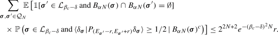
where \( {{\mathbb {P}}}( \cdot \vert B_{\alpha N}(\pmb {\sigma })^c ) \) denotes the conditional expectation, conditioned on all random variables aside from those in \( B_{\alpha N}(\pmb {\sigma }) \) and \( P_I \) is still the spectral projection of \( H_{\alpha N}(\pmb {\sigma }) \) onto I. The last inequality resulted from an application of the bound from 1. to the conditional expectation.\(\square \)


4.4 Proof of Theorem 1.5
The proof of Theorem 1.5 makes use of the deep-hole geometry of the REM. If U satisfies a global \( (\varepsilon ,\delta ,\alpha ) \)-deep hole scenario, we study the auxiliary Hamiltonian
with operators \( H_{\alpha N}(\pmb {\sigma }) \), whose action is restricted to the non-intersecting balls \( B_{\alpha N}(\pmb {\sigma }) \) around extremal sites \( \pmb {\sigma } \in {\mathcal {L}}_{\beta _c-\delta } \). These operator have been introduced and studied in Sect. 4.2. The remainder \(H_r\) is that part of H which purely belongs to the complement of the union of balls,
The difference between the Hamiltonian of interest \(H = \Gamma T + U \) and the auxiliary \(H^\prime \) is
It describes the hopping between the balls and the complementary configuration space, i.e.,
The norm of A can be bounded as follows
where the last equality is (2.2). It is easy to see that \( \Vert A \Vert \) is indeed of order N. However, for energies below \( E_\delta = -N (\beta _c - \delta ) \), the perturbation is of a much smaller magnitude. This is the basic idea in the proofs of our main results for the localization regime. As a preparation, we also need the following result, which is implicitly contained in [52].
Proposition 4.5
(cf. [52]). For all \( \Gamma , \delta > 0 \) the truncated Hamiltonian \( H :=\Gamma T + U \mathbb {1}_{U \ge -(\beta _c-\delta ) N } \) acting on \( \ell ^2({\mathcal {Q}}_N) \) is lower bounded by
except for an event of exponentially small probability.
Proof of Theorem 1.5
We only study the joint event \( \Omega _N(\Gamma ,\delta ,\alpha ) \) on which i) the bound in Proposition 4.5 applies, and ii) U satisfies a global \( (\varepsilon ,\delta ,\alpha ) \)-deep hole scenario with parameters
and \( \alpha > 0\) small enough such that (4.1) and \( 2 \Gamma \sqrt{\alpha (1-\alpha ) } < \delta /8 \), and hence in particular (4.7) is satisfied. Together with Lemma 4.2 this ensures that \( \Omega _N(\Gamma ,\delta ,\alpha )\) occurs with a probability of at least \( 1 - e^{- c N} \) with at some \( c \equiv c(\Gamma , \delta ,\alpha ) > 0 \). Moreover:
-
1.
From Lemma 4.3 we learn that for any \(\pmb {\sigma } \in {\mathcal {L}}_{\beta _c-\delta } \) the spectrum \( {{\,\textrm{spec}\,}}H_{\alpha N}(\pmb {\sigma }) \) below \( E_\delta = - N (\beta _c -\delta ) \) consists of just one eigenvalue \( E_{\pmb {\sigma }} = \inf {{\,\textrm{spec}\,}}H_{\alpha N }(\pmb {\sigma }) \), which is given by (4.8) with an error term \({\mathcal {O}}_{\Gamma ,\delta }\left( N^{-1/4} \right) \) uniformly for all \( \pmb {\sigma } \in {\mathcal {L}}_{\beta _c-\delta } \).
-
2.
By the variational principle and the natural embedding of Hilbert spaces, the ground state energy of \(H_r\) is bounded from below by that of \( \Gamma T + U \mathbb {1}_{U \ge -(\beta _c-\delta ) N } \) on \( \ell ^2({\mathcal {Q}}_N) \). The lower bound in Proposition 4.5 then shows that
$$\begin{aligned} \inf {{\,\textrm{spec}\,}}H_r \ge - N \left( \beta _c - \delta +o_{\Gamma ,\delta }(1) \right) . \end{aligned}$$
Hence, \( H_r \) does not contribute to the low-energy spectrum of \( H' \) below \( E_{\delta /2} = -N (\beta _c - \delta /2) \) for all N large enough. Moreover, the spectral projection \( P_{\delta } :=\mathbb {1}_{(-\infty ,E_{\delta /2} )}(H^\prime ) \) can be written as
in terms of rank-one projections of the \( \ell ^2 \)-normalized ground states \( \psi _{\pmb {\sigma }} \) of \( H_{\alpha N}(\pmb {\sigma }) \). We thus conclude for some \( C = C(\Gamma ,\delta ) < \infty \), and \( c = c(\alpha ) > 0 \)
where the inequalities follow from (4.21) and (4.10) together with the fact that \(A_{\pmb {\sigma }}\) only acts on the part of \(\psi _{\pmb {\sigma }}\) on \(S_{\alpha N}(\pmb {\sigma })\).
We then rewrite H using the block decomposition of \( \ell ^2({\mathcal {Q}}_N) \) induced by \( P_{\delta } \) and \( Q_\delta :=1-P_{\delta } \) and again employ the Schur complement method. Since \( H^\prime \) is diagonal in this decomposition and its \( Q_{\delta } \) projection has a spectrum above the threshold energy \( E_{\delta /2} \), it remains to investigate the blocks of the perturbation \( \Gamma A \):
-
1.
Since \( P_\delta \) is supported entirely on the balls, the first diagonal term vanishes, i.e. \( P_\delta A P_\delta = 0 \). The operator norms of the off-diagonals \( \Vert P_\delta A (1-P_\delta ) \Vert \le \Vert A P_{\delta } \Vert \) are exponentially small by (4.23).
-
2.
The operator \(Q_{\delta } A Q_{\delta } \) is bounded from below by \( - \Vert A\Vert \) which is estimated in (4.21). We thus conclude that for all N large enough:
$$\begin{aligned} Q_\delta H^\prime + Q_{\delta } A Q_{\delta }&\ge E_{\delta /2} - \Vert A\Vert \ge -N \left( \beta _c - \delta /2 + 2 \Gamma \sqrt{\alpha (1-\alpha )} +o_{\Gamma ,\alpha }(1) \right) \\ {}&\ge -N \left( \beta _c - \delta /4 \right) . \end{aligned}$$Consequently, the Schur complement matrix
$$\begin{aligned} S_\delta (E):= \left( Q_\delta H^\prime + Q_{\delta } A Q_{\delta } - E \right) ^{-1} \end{aligned}$$is well defined on \( Q_\delta \ell ^2({\mathcal {Q}}_N) \) and bounded, \( \Vert S_\delta (E) \Vert \le (E_{\delta /4}-E)^{-1} \) for any \( E < E_{\delta /4} \).
The spectrum of H below \( E_{\delta /4} = -N \left( \beta _c - \delta /4 \right) \) is thus characterized using Schur’s method, which yields:
-
1.
\( E < E_{\delta /4}\) is an eigenvalue of H if and only if \( E \in {{\,\textrm{spec}\,}}\left( P_\delta H' - P_\delta A S_\delta (E) A P_{\delta } \right) \).
-
2.
The \( \ell ^2 \)-normalized eigenvector \( \psi \) corresponding to E and H satisfies:
$$\begin{aligned} (P_\delta H' - E P_\delta ) \psi&= P_\delta A S_\delta (E) A P_{\delta } \psi \nonumber \\ Q_\delta \psi&= - S_\delta (E) A P_\delta \psi . \end{aligned}$$(4.24)
We now proceed with the completion of the proof of the assertion on the spectrum and eigenvectors separately.
Spectrum: The spectrum of H below \( E_{\delta /8} \) is determined through the above Schur complement method. Since for all \( E \le E_{\delta /8} \) at at some \( C = C(\Gamma ,\delta ) < \infty \) and \( c = c(\alpha ) > 0 \)
the eigenvalues below \( E_{\delta /8} \) thus coincide with the eigenvalues of \( P_\delta H' \) below this energy up to an error, which is exponentially small in N [13, Corollary 3.2.6]. Since the eigenvalues of \( P_\delta H' \) are given by (4.8), the assertion in Theorem 1.5 follows.
Eigenvectors: We concentrate our attention on energies below \( E_s = - N (\beta _c- s ) \) with \( s \in (0, \delta /8] \) small enough such that \( 2 \beta _c s < c \) with the decay rate \( c > 0 \) from (4.25). This ensures that \( e^{-\alpha c N} < e^{-2 \beta _c s N} {=}{:}r(s) \) for all sufficiently large N. According to the spectral averaging Lemma 4.4, since \( s \le \delta /8 \) and the condition (4.7) is monotone in \( \delta \), the event
has probability of at least \( 1 - 4 e^{- s^2 N } - e^{-c N} \) for some \( c > 0 \). We may therefore assume its occurrence.
Perturbation theory based on the above Schur complement analysis and (4.25) (combined with the characterization of eigenvalues established in Theorem 1.5) then guarantees that the eigenvector \( \psi \) of H corresponding to the eigenvalue \( E= U(\pmb {\sigma }) + \Gamma ^2 N/U(\pmb {\sigma }) + {\mathcal {O}}(N^{-1/4}) \), which is uniquely characterized by \( \pmb {\sigma } \in {\mathcal {L}}_{\beta _c-s} \), is norm-close to the ground-state eigenvector \( \psi _{ \pmb {\sigma }} \) of \( H_{\alpha N}(\pmb {\sigma }) \), i.e.,
Here, the inequalities combine (4.24)–(4.26). The rest of the claim on the \( \ell ^2 \)-estimates of the eigenvectors then follows from the respective properties of \( \psi _{ \pmb {\sigma }} \) established in Lemma 4.3. The event \(\Omega _{N,\Gamma ,\delta }^loc \) is then defined by specifying a value for \(\alpha _0 = \alpha _0(\Gamma ,\delta )\) and intersecting \( \Omega _N(\Gamma ,\delta ,\alpha _0)\) with (4.26). \(\square \)
4.5 Proof of Theorem 1.7
All assertions concerning the \( \ell ^2 \)-properties of the ground-state can easily be collected from the proof of Theorem 1.5.
Proof of Theorem 1.7 (\( \ell ^2 \)-properties). According to Theorem 1.5 for all events aside from one of exponentially small probability, there is some \( \pmb {\sigma }_0 \in {\mathcal {Q}}_N \) such that the ground state eigenvector is approximated by \( \Vert \psi - \delta _{\pmb {\sigma }_0 }\Vert _{\ell ^2}^2 = {\mathcal {O}}_{\Gamma }\left( \frac{1}{N}\right) \). The estimate \({\mathcal {O}}_{\Gamma }\left( \frac{1}{N}\right) \) does not depend on \(\delta \) anymore as we may fix \(\delta \), if we only consider the ground state. This will be always assumed in the following. Moreover, the ground-state energy is \( E = U(\pmb {\sigma }_0 ) + \frac{\Gamma ^2 N}{U(\pmb {\sigma }_0 )} + {\mathcal {O}}_{\Gamma }\left( N^{-1/4} \right) \), where \( U(\pmb {\sigma }_0 ) \) is one of the REM’s extremal energies for which we may assume that
at the expense of excluding another event of exponentially small probability stemming from deviations to the known extremal statistics of the REM, cf. (1.7).
It thus remains to establish the assertion on the first order perturbation \( \xi \in \ell ^2({\mathcal {Q}}_N) \). That \(\langle \xi \vert H \xi \rangle \) agrees with the ground state energy up to order \(o_\Gamma (1)\) is a result of a simple calculation and a comparison with the above formula for E. It remains to prove \(\Vert \psi - \xi \Vert ^2 = {\mathcal {O}}_{\Gamma }(N^{-2})\). To this end, we revisit the proof of Theorem 1.5. From the validity of the global \((\beta _c/2,\delta ,\alpha ) \)-deep hole scenario specified there and in view of (4.9), it suffices to show
For a proof of these assertions, we use the eigenvalue equation (4.16) on \( S_1(\pmb {\sigma }_0) \) together with \(\psi ({\pmb {\sigma }_0}) = 1+ {\mathcal {O}}_{\Gamma }(N^{-1})\). If we pick \( \pmb {\sigma } \in S_1(\pmb {\sigma }_0) \), this yields
Here the last step also relied on the estimate \( \vert U(\pmb {\sigma })\vert \le \varepsilon N \) valid in the \((\varepsilon ,\delta ,\alpha ) \)-deep hole scenario, as well as (4.28). With a suitable constant \( C = C(\Gamma ) < \infty \), we then have
An exponential Chebychev-Markov estimate leads to \({{\mathbb {P}}}( N^{-2} \sum _{\pmb {\sigma } \in S_1(\pmb {\sigma }_0 )} (U(\pmb {\sigma })^{2} - N) ) \ge 1) \le e^{-c N} \) for some \( c >0\). Thus, except for an event of exponentially small probability the second claim in (4.29) holds. Since \(\psi \) is \( \ell ^2\)-normalized, this leads to
which readily implies the first claim in (4.29).
For a proof of the \( \ell ^1 \)-estimate on the ground state eigenfunction, we need to sharpen estimates on the large-deviation geometry of the REM. To this end we define for \(\varepsilon , \delta > 0\) the following tripartition of the Hamming cube:
A modification of ideas used in the proof of Lemma 4.2 and [51, Lemma 2] yields:
Lemma 4.6
For any \(\varepsilon > 0\) there exist \(K = K(\varepsilon ) \in {{\mathbb {N}}}\) and a family of events \(\Omega _{\varepsilon , N}\) such that for N large enough
-
(i)
For any \(\pmb {\sigma } \in A_2(\varepsilon , \delta ) \cup A_3(\delta ) \): \( \displaystyle \vert B_4(\pmb {\sigma }) \cap (A_2(\varepsilon , \delta ) \cup A_3(\delta )) \vert \le K \) on \(\Omega _{\varepsilon , N}\).
-
(ii)
\({{\mathbb {P}}}(\Omega _{\varepsilon , N}) \ge 1 - 2^{-N}\).
Proof
Let \(\Omega _{\varepsilon , N,K}\) be the event, where the assertion (i) holds true with constant K. It remains to show that the complement satisfies \({{\mathbb {P}}}(\Omega _{\varepsilon , N,K}^{c}) \le 2^{-N}\) for an appropriate choice for K and N large enough. To this end we estimate
Here the second line is a consequence of the union bound and the third line follows from the independence and a simple counting argument. Choosing \(K > 4 \ln 2/\varepsilon ^2\), we see that \({{\mathbb {P}}}(\Omega _{\varepsilon , N,K}^{c}) < 2^{-N}\) for N large enough. \(\square \)
As a final preparation, we also need the following elementary observation on the size of large deviation sites.
Lemma 4.7
For any \( \delta \in (0,\beta _c) \) and all N:
Proof
The cardinality \(\vert A_3(\delta )\vert \) is a sum of \(2^N \) independent Bernoulli variables with success probability \( p = {{\mathbb {P}}}(\vert U(\pmb {\sigma })\vert > (\beta _c - \delta ) N) \le 2 e^{-\frac{1}{2} (\beta _c - \delta )^2 N} \) such that \( {\mathbb {E}}[\vert A_3((\delta ))\vert ] = 2^N p \). The claim thus follows from a standard Markov estimate. \(\square \)
We are finally ready to finish the proof of our main result in the localization regime.
Proof of Theorem 1.7\( (\ell ^p \)-properties). We first observe that the claims on the \(\ell ^p\)-norms immediately follow from the \(\ell ^1\)-norm asymptotics (1.25). To see this, recall that \(\psi (\pmb {\sigma }_0 ) = 1 + o_{\Gamma }(1)\) for some \( \pmb {\sigma }_0 \in {\mathcal {Q}}_N \), and that \(\psi (\pmb {\sigma }) \le c \, N^{-1}\) for all \(\pmb {\sigma } \ne \pmb {\sigma }_0\). Hence for any \(1< p < \infty \):
It therefore remains to establish (1.25).
Recalling that the ground state wavefunction \(\psi \) is positive, we can write \( \Vert \psi \Vert _{\ell ^1} = \sum _{\pmb {\sigma }} \psi (\pmb {\sigma }) \). The eigenvalue equation for \(\psi \) leads to
The second equality follows from the fact that each \(\pmb {\sigma }\) has N neighbors. The main idea is now to show that the remainder term \( \sum _{\pmb {\sigma } \ne \pmb {\sigma }_0} U(\pmb {\sigma }) \psi (\pmb {\sigma })\) can be controlled by the other two terms on the right side. Here, we use the tripartition \(A_1(\varepsilon ), A_2(\varepsilon ,\delta ), A_3(\delta )\) of the configuration space and bound the contribution of each \(A_i\) separately.
In the following, we fix \( \delta , \alpha > 0 \) small enough, such that the REM satisfies a global \( (\beta _c/2,\delta ,\alpha ) \)-deep hole scenario with a probability which is exponentially close to one. Moreover, we pick \( \varepsilon > 0 \) arbitrary and fix \( K=K(\varepsilon ) \in {\mathbb {N}} \) the assertions of Lemma 4.6 hold on a joint event on which the global \( (\beta _c/2,\delta _0,\alpha _0 ) \)-deep hole scenario applies as well. This event still has a probability of at least \( 1 - e^{-c(\delta ,\alpha ) N } \) with some \( c(\delta ,\alpha ) > 0 \), which is independent of \( \varepsilon \).
Contribution of \(A_1(\varepsilon )\): In this case we use the trivial estimate, \( \left| \sum _{\pmb {\sigma } \in A_1} U(\pmb {\sigma }) \psi (\pmb {\sigma })\right| \le \varepsilon N \Vert \psi \Vert _{\ell ^1} \).
Contribution of \(A_3(\delta )\): We only consider \(\delta \le \delta _0\), such that sites \(\pmb {\sigma } \in A_3(\delta ) {{\setminus }}\{\pmb {\sigma }_0\}\) lie outside the ball \(B_{\alpha _0 N}(\pmb {\sigma }_0)\). In particular, there is some \(c > 0\) such that for all N large enough and all \(\pmb {\sigma } \in A_3(\delta ) {{\setminus }}\{\pmb {\sigma }_0\}\) the ground state is uniformly bounded, \(\vert \psi (\pmb {\sigma })\vert \le e^{-cN}\). We now pick \( \delta :=\min \{\delta _0, c/(4 \beta _c) \}\) and shrink the considered event such that \( \vert A_3(\delta )\vert \le 2 \ e^{N c/4} \). According to Lemma 4.7 this event still has a probability greater than \( 1 - e^{-c(\delta ,\alpha ) N } \) with some \( c(\delta ,\alpha ) > 0 \). On this event, we conclude for all N large enough
Contribution of \(A_2(\varepsilon ,\delta )\): We first consider the configurations in \(A_2(\varepsilon ,\delta )\) close to the center \(\pmb {\sigma }_0\), which we estimate for N large by
with some \(C = C(\Gamma )\). We use \( \vert U(\pmb {\sigma })\vert \le \beta _c N/2 \) due to the validity of the global \( (\beta _c/2,\delta ,\alpha ) \)-deep hole scenario as well as the pointwise bound \(\psi (\pmb {\sigma }) \le C N^{-1} \) for all \( \pmb {\sigma } \in B_4(\pmb {\sigma }_0) \) with \(\pmb {\sigma } \ne \pmb {\sigma }_0 \).
It remains to consider \(\pmb {\sigma } \in A_2(\varepsilon ,\delta ) {{\setminus }} B_4(\pmb {\sigma }_0)\). The eigenvalue equation reads
Since \(E \le (\beta _c - \delta /2) N\) for N large enough, we obtain for \(\pmb {\sigma } \in A_2(\varepsilon ,\delta )\) the bound
The essence of the following argument is that the value of any \(\psi (\pmb {\sigma })\) is comparable to the mean on the corresponding \(S_1(\pmb {\sigma })\) sphere and, thus, \(\psi \) cannot take especially large values on \(A_2(\varepsilon ,\delta )\). To make this intuition precise, we separate the \(A_3(\delta )\) configurations, which we possibly encounter in the spherical mean and repeat the procedure for the remaining \(\pmb {\sigma }^\prime \in S_1(\pmb {\sigma })\). This leads to
which for N large enough implies
We now further shrink the considered event to ensure that \(\Vert U\Vert _\infty \le 2 \beta _c N\) holds true. This happens for all but an event of exponentially probability, cf. (1.6). Thus, for N large enough
In the third line we used the observation that each configuration \(\pmb {\sigma } \in {\mathcal {Q}}_N\) appears in the summation at most K times due to Lemma 4.6. The last step is a consequence of our exponential bound on \( \psi (\pmb {\sigma }) \) on the \(A_3(\delta )\)-configurations.
Combining the partial results on each \(A_J\), we arrive with some \(C = C(\Gamma )\) at the bound
which is valid on with probability of at least \( 1- e^{-c N } \) with some \( c > 0 \) which in independent of \(\varepsilon \). Since \(\varepsilon > 0 \) was arbitrary, the claimed convergence now follows from (4.30).
5 Free Energy Asympotics
For our proof of Theorem 1.10 we exploit that the partition function is determined by the eigenvalues close to the thermal averages
depending on the phase. To determine their behavior we consider the local region around \(\pmb {\sigma } \in {\mathcal {L}}_{\varepsilon }\), where \( \varepsilon > 0 \) has to be allowed to be arbitrarily small. In this case, we cannot guarantee anymore that all balls \(B_R(\pmb {\sigma })\) are disjoint. However, we will show that this is still true for isolated extremal sites \(\pmb {\sigma } \in {\mathcal {L}}_{\varepsilon }\), which are in the majority. Then, we establish the order-one corrections of Theorem 1.5 for those isolated large deviations. Based on these results, we prove Theorem 1.10 via a suitable approximation argument using auxiliary operators on cut domains of the configuration space.
5.1 Basic large deviations
We first record some standard facts in the statistical mechanics of the pure REM and pure paramagnet.
Proposition 5.1
-
1.
For any \(\beta \ge 0\) we have \( \langle T \rangle ^{\text {pm}}_\beta = - N \tanh \beta \). Moreover, for any \(\beta \ge 0, \delta > 0\) there exists some \(c = c(\beta ,\delta ) > 0\) such that
$$\begin{aligned} \frac{ {{\text {Tr}}\,}\mathbb {1}_{[-N(\tanh \beta + \delta ),-N(\tanh \beta - \delta ) ]}(T) e^{-\beta T}}{{{\text {Tr}}\,}e^{-\beta T}} \ge 1 - e^{-cN}. \end{aligned}$$(5.2) -
2.
For \(\beta < \beta _c\) we have almost surely \( \langle U \rangle ^{\text {cl}}_\beta = - (\beta + o(1)) N \). Moreover, for \(\beta < \beta _c \) and \( \delta > 0\) there exists some \(c = c(\beta ,\delta ) > 0\) such that
$$\begin{aligned} \frac{ {{\text {Tr}}\,}\mathbb {1}_{[-N(\beta + \delta ),-N( \beta - \delta ) ]}(U) e^{-\beta U}}{{{\text {Tr}}\,}e^{-\beta U}} \ge 1 - e^{-cN} \end{aligned}$$(5.3)except for an exponentially small event.
-
3.
For \(\beta > \beta _c\) we have almost surely \( \langle U \rangle ^{\text {cl}}_\beta = - (\beta _c + o(1)) N \). Moreover, for \(\beta > \beta _c \) and \( \delta > 0\) there exists some \(c = c(\delta ) > 0\) such that
$$\begin{aligned} \frac{ {{\text {Tr}}\,}\mathbb {1}_{(-\infty ,-N( \beta _c - \delta ) ]}(U) e^{-\beta U}}{{{\text {Tr}}\,}e^{-\beta U}} \ge 1 - e^{-cN}. \end{aligned}$$(5.4)
The proof for the expressions of the thermal averages \(\langle T \rangle ^{\text {pm}}_\beta , \langle U \rangle ^{\text {cl}}_\beta \) is by differentiating the explicit formulas for the pressure with respect to \(\beta \). The results on the concentration of the Gibbs measure are then of Cramér type and follow from the usual convexity estimates of the (explicit) free energy.
5.2 Spectral analysis on clusters
In the proofs of Theorem 1.5 and 1.7 we derived the order-one correction of the energy levels \(U(\pmb {\sigma })\) caused by extremal sites \(\pmb {\sigma } \in {\mathcal {L}}_{\varepsilon }\) with \( \varepsilon \approx \beta _c \) from a local analysis on non-overlapping balls \(B_R(\pmb {\sigma })\) of some radius R. For the proof of Theorem 1.10 however, we need good control on all eigenvalues with energy below \( - \varepsilon N \) with \( \varepsilon > 0 \) arbitrary and, thus, the large deviation set \({\mathcal {L}}_{\varepsilon }\) has to be considered for any \(\varepsilon >0\). The balls \(B_R(\pmb {\sigma })\) then have a nonempty intersection and the aim of this subsection is to deal with this modified situation. Let us introduce some definitions and notation.
Definition 5.2
Let \(\varepsilon > 0\) and \( k \in {\mathbb {N}}_0 \). We denote \( \pmb {\sigma } \overset{k}{\sim }\ \pmb {\sigma }^\prime \iff d(\pmb {\sigma },\pmb {\sigma }^\prime ) \le 2k +2 \). We call a set \( G \subset {\mathcal {L}}_{\varepsilon }\) \((k,\varepsilon )\)-connected (with respect to \( \overset{k}{\sim }\ \)) if for any \(\pmb {\sigma },\pmb {\sigma }^\prime \in G\) there exists a sequence \(\pmb {\sigma } = \pmb {\sigma }^{(0)}, \pmb {\sigma }^{(1)}, \cdots , \pmb {\sigma }^{(m)} = \pmb {\sigma }^{\prime }\) such that \(\pmb {\sigma }^{(i)} \in G\) and \(\pmb {\sigma }^{(i)} \overset{k}{\sim } \pmb {\sigma }^{(i+1)}\) for all \( 0 \le i \le m-1\). If \(G \subset {\mathcal {L}}_{\varepsilon }\) is \((k,\varepsilon )\)-connected and for any \((k,\varepsilon )\)-connected \(G^\prime \) with \(G \subset G^\prime \subset {\mathcal {L}}_{\varepsilon }\) it follows \(G = G^\prime \), we call G a \((k,\varepsilon )\)-component. We denote the family of \((k,\varepsilon )\)-components of \({\mathcal {L}}_{\varepsilon }\) by \({\mathcal {G}}_{k,\varepsilon }\).
We call \(\pmb {\sigma } \in {\mathcal {Q}}_N\) \((k,\varepsilon )\)-isolated if \(G = \{\pmb {\sigma } \} \in {\mathcal {G}}_{k,\varepsilon } \) and \(I_{k,\varepsilon }\) denotes the collection of \((k,\varepsilon )\)-isolated configurations.
The case \(k=0\) coincides with the notion of ’gap-connected’ used in [50,51,52].
The extremal set \({\mathcal {L}}_{\varepsilon }\) naturally decomposes in its components, i.e., \({\mathcal {L}}_{\varepsilon } = \cup _{G \in {\mathcal {G}}_{k,\varepsilon } } G\). We define for each \((k,\varepsilon )\)-component G the corresponding cluster
By construction \(d(C_k(G),C_k(G^\prime )) \ge 2\) for different k-components \(G \ne G^\prime \).
We start with a combinatorial lemma which shows that the size of \((k,\varepsilon )\)-components remains bounded and that most \((k,\varepsilon )\)-components are isolated.
Lemma 5.3
Let \(\varepsilon > 0\) and \(k \in {{\mathbb {N}}}_0\) be fixed, but arbitrary.
-
1.
There exists an \(M = M(k,\varepsilon ) \in {{\mathbb {N}}}\) such that
$$\begin{aligned} \Omega _{N,M}(\varepsilon ,k) :=\left\{ \max _{G \in {\mathcal {G}}_{k,\varepsilon }} \vert G\vert \le M \right\} . \end{aligned}$$(5.5)occurs with probability \( {{\mathbb {P}}}( \Omega _{N,M}(k,\varepsilon ) ) \ge 1 - e^{-c N} \) for some \( c > 0 \).
-
2.
Let \( \varepsilon< a < b\) and \(b < \beta _c\). Then for all events, but one of exponentially small probability:
$$\begin{aligned} \frac{ \vert {\mathcal {L}}_{a,b} \cap I_{k,\varepsilon }^{c} \vert }{\vert {\mathcal {L}}_{a,b}\vert } \le e^{-\varepsilon ^2 N/4}, \end{aligned}$$(5.6)where \( {\mathcal {L}}_{a,b} :={\mathcal {L}}_{a} \cap {\mathcal {L}}_{b}^{c} \) and \( (\cdot )^c \) indicates the complement of that set.
-
3.
Let \(a = \beta _c - \delta \) and suppose that \( \delta (2 \beta _c-\delta ) < \varepsilon ^2\). Then, besides of an exponentially small event
$$\begin{aligned} {\mathcal {L}}_{a} \cap I_{k,\varepsilon }^{c} = \emptyset . \end{aligned}$$(5.7)
Proof
For a proof of the first assertion, we estimate for any \( M \in {\mathbb {N}} \) using a union bound
As the binomial coefficient is a polynomial in N the claim follows for \(M > 2 \ln 2/ \varepsilon ^2\).
For a proof of the second assertion, we rewrite \( \vert {\mathcal {L}}_{a,b}\vert = \sum _{\pmb {\sigma }} Z_{\pmb {\sigma }} \), where \(Z_{\pmb {\sigma }}\) are i.i.d. Bernoulli variables with success probability
Since \( b < \beta _c\), the average size \( {\mathbb {E}}[\vert {\mathcal {L}}_{a,b}\vert ] = 2^N p_N \) is exponentially large and, by a Markov estimate, the same applies to all events aside from one of super-exponentially small probability, i.e., \( {{\mathbb {P}}}(\vert {\mathcal {L}}_{a,b}\vert \le 2^{N-1} p_N ) \le e^{-e^{C N}} \) for some \( C > 0 \). Similarly, the conditional probability \( {\mathbb {P}}_{\pmb {\sigma }}:= {\mathbb {P}}\left( \cdot \vert \{ \pmb {\sigma } \}^c \right) \) of the configuration to not be \((\varepsilon ,k) \)-isolated equals the probability to find on \(B^{o}_{2k+2} :=B_{2k+2}(\pmb {\sigma } )\backslash \{ \pmb {\sigma }\} \) another large deviation in \({\mathcal {L}}_{\varepsilon }\) and hence \( {\mathbb {P}}_{\pmb {\sigma }}(\exists \ \pmb {\sigma }^\prime \in I_{k,\varepsilon }^c\cap B^{o}_{2k+2} ) \le \vert B_{2k+2}\vert e^{-N \varepsilon ^2/2} \le N^{2k+2} e^{-N \varepsilon ^2/2 } \) by the union bound and the Gaussian-tail estimate. This allows us to estimate

with \(p_N \) from (5.8). Excluding the event on which \( \vert {\mathcal {L}}_{a,b}\vert \le 2^{N-1} p_N \), we thus arrive at
by a Chebychev-Markov estimate. Inserting the bound (5.9) completes the proof.
For the last assertion, we note that by Lemma 4.2 the condition on \(\delta \) implies that for \(\alpha > 0\) small enough a global \((\varepsilon ,\delta ,\alpha )\)-deep hole scenario occurs with probability exponentially close to one. \(\square \)
The next lemma establishes the spectral properties of the restriction \(H_{C_k(G)}\) of the QREM Hamiltonian to the Hilbert space \( \ell ^2(C_k(G)) \) of a cluster corresponding to \(G \in {\mathcal {G}}_{k,\varepsilon }\). For its formulation, we define for \( \delta > 0 \) the spectral projections
Recall the events \( \Omega _N^{u} \) defined in (4.3) and \( \Omega _{N,M}(k,\varepsilon ) \) defined in (5.5).
Lemma 5.4
Let \(\varepsilon > 0\) and \(k\ge 2 \). On the event \( \Omega _N^{u} \cap \Omega _{N,M}(\varepsilon ,k) \) the following assertions are valid for all N large enough:
-
1.
\( \displaystyle \max _{G \in {\mathcal {G}}_{k,\varepsilon }} \Vert H_{C_k(G)} - U_{C_k(G)} \Vert = {\mathcal {O}}_{\Gamma ,k,M}(\sqrt{N}) \).
-
2.
If \(\psi \) is an \( \ell ^2 \)-normalized eigenfunction of \(H_{C_k(G)}\) with \(\langle \psi , \, H_{C_k(G)}\psi \rangle \le - \frac{3}{2} \varepsilon N\), we have
$$\begin{aligned} \vert \psi (\pmb {\sigma })\vert = {\mathcal {O}}_{\Gamma ,k,M,\varepsilon }( N^{-{{\,\textrm{dist}\,}}(G,\pmb {\sigma })}), \end{aligned}$$(5.10)and
$$\begin{aligned} \Vert \mathbb {1}_{C_k(G)\backslash G }\psi \Vert ^2 = {\mathcal {O}}_{\Gamma ,k,M,\varepsilon }(N^{-1}), \qquad \Vert \mathbb {1}_{\partial C_k(G)}\psi \Vert ^2 = {\mathcal {O}}_{\Gamma ,k,M,\varepsilon }(N^{-k}), \end{aligned}$$(5.11)where \(\mathbb {1}_{\partial C_k(G)}\) is the natural projection onto the boundary of \(C_k(G)\). In particular, all estimates are independent of \( \psi \) and G.
-
3.
\( \displaystyle \sup _{ G\in {\mathcal {G}}_{k,\varepsilon }} \sup _{\pmb {\sigma } \in {\mathcal {L}}_{2 \varepsilon } \cap G} \langle \delta _{\pmb {\sigma }} \vert Q_{3 \varepsilon /2}(G) \delta _{\pmb {\sigma }} \rangle = {\mathcal {O}}_{\Gamma ,k,M,\varepsilon }(N^{-1}) \).
-
4.
If \(G = \{\pmb {\sigma _0} \}\) is \((k,\varepsilon )\)-isolated and \(U(\pmb {\sigma }_0) \le - 2\varepsilon N\), then the ground state energy of \(H_{C_k(G)}\) is given by
$$\begin{aligned} E_{\pmb {\sigma _0}} :=\inf {{\,\textrm{spec}\,}}H_{C_k(G)} = U(\pmb {\sigma }_0) + \frac{\Gamma ^2 N}{ U(\pmb {\sigma }_0)} + {\mathcal {O}}_{\Gamma ,k,\varepsilon }(N^{-1/4}). \end{aligned}$$(5.12)
Proof
-
1.
We write \(H_{C_k(G)} = U_{C_k(G)} + \Gamma T_{C_k(G)}\) and recall that \(C_k(G)\) is a union of at most M Hamming balls \(B_k(\pmb {\sigma })\) with \( \pmb {\sigma } \in G \). Thus, by the triangle inequality and Proposition 2.1 we obtain \( \Vert T_{C_k(G)}\Vert \le M c_k \sqrt{N} \), and hence the claim.
-
2.
We introduce the modified spheres \(S_r(G)\) for \(0 \le r \le k\),
$$\begin{aligned} S_r(G) :=C_r(G) {\setminus } C_{r-1}(G) = \{ \pmb {\sigma } \in C_k(G) \, \vert \, \text {dist}(\pmb {\sigma },G) = r \} \end{aligned}$$and for the eigenvector \( \psi \) the maximal values on the spheres, \( s_r :=\max _{\pmb {\sigma } \in S_r(G)} \vert \psi (\pmb {\sigma })\vert \). We use the convention \(S_0(G) = G\) and note that \(S_k(G) = \partial C_k(G)\). Moreover, we observe that for any \(\pmb {\sigma } \in S_r(G)\) and \(1 \le r \le k\):
$$\begin{aligned} \begin{aligned} \vert S_1(\pmb {\sigma }) \cap S_r(G)\vert \le M, \qquad r&\le \vert S_1(\pmb {\sigma }) \cap S_{r-1}(G)\vert \le r M, \\ \quad N - (r+1)M&\le \vert S_1(\pmb {\sigma }) \cap S_{r+1}(G)\vert \le N - r. \end{aligned} \end{aligned}$$We now use the eigenvalue equation
$$\begin{aligned} - E \psi (\pmb {\sigma }) = \Gamma \sum _{\pmb {\sigma }^\prime \in S_1(\pmb {\sigma })} \psi ( \pmb {\sigma }^\prime ) - U(\pmb {\sigma }) \psi (\pmb {\sigma }), \end{aligned}$$to derive the claimed decay estimate. Inserting the above geometric bounds into the eigenvalue equation, we obtain for all \( 1 \le r \le k \) with the convention \( s_{k+1} = 0 \):
$$\begin{aligned} - E s_r \le \Gamma rM s_{r-1} + \Gamma (N-r) s_{r+1} + (\varepsilon N + \Gamma M) s_r. \end{aligned}$$(5.13)We claim that for all \( 1 \le r \le k \) and N large enough
$$\begin{aligned}s_r \le \frac{2 M \Gamma k }{\vert E\vert -\varepsilon N - \Gamma M} s_{r-1}.\end{aligned}$$This is immediate from (5.13) in case \( r = k \) (even without the factor 2). In case \( 1 \le r < k \), the bound is proven recursively. If the inequality holds for \( r+1 \), then (5.13) implies
$$\begin{aligned} \vert E\vert s_r \le \Gamma rM s_{r-1} + \left( \frac{2 N \Gamma ^2 k }{\vert E\vert -\varepsilon N - \Gamma M } + \varepsilon N + \Gamma M \right) s_r, \end{aligned}$$and hence the claimed inequality for all N large enough. Since \(s_0 \le 1\), this establishes (5.10) by iteration.
The first claim in (5.11) follows from (5.10) using \( \vert G\vert \le M \). Indeed, for some \(C = C(\Gamma ,k,M,\varepsilon )\)
$$\begin{aligned} \sum _{\pmb {\sigma } \ne \pmb {\sigma }_0} \vert \psi (\pmb {\sigma })\vert ^2 \le C \sum _{r=1}^K N^{-2r} \left| \{ \pmb {\sigma } \, \vert \,{{\,\textrm{dist}\,}}(\pmb {\sigma },G) = r \} \right| \le C M \, \sum _{r=1}^K N^{-r} =\frac{C M}{N-1}. \end{aligned}$$Since \(\vert \partial C_k(G)\vert \le M N^k\) the second inequality in (5.11) follows similarly.
-
3.
We will repeatedly make use of a coupling principle which follows from 1., namely the fact that the eigenvalues of \(H_{C_k(G)} \) and \( U_{C_k(G)} \) agree up to a uniform error of order \( {\mathcal {O}}_{\Gamma ,k,M}(N^{1/2}) \). Since \(\vert {\mathcal {L}}_\varepsilon \cap G \vert \le \vert G\vert \le M\), this implies that \( \dim P_{3\varepsilon /2}(G) \le M\) for any component \(G \in {\mathcal {G}}_{k,\varepsilon }\) if N is chosen large enough. By the pigeon-hole principle, for any component G we find some \(a = a(G) \in [3 \varepsilon /2, 2 \varepsilon ] \) such that
$$\begin{aligned} P_{a - \varepsilon /(2M)}(G) - P_{a + \varepsilon /(2M)}(G) = \mathbb {1}_{(-(a+\varepsilon /(2M))N,- (a-\varepsilon /(2M))N}(H_{C_k(G)}) = 0.\nonumber \\ \end{aligned}$$(5.14)Since \( Q_{3 \varepsilon /2}(G) \le Q_a(G)\), it is enough to prove the assertion with \( Q_{3 \varepsilon /2}(G) \) replaced by \( Q_a(G) \).
To this end, we fix a component \(G \in {\mathcal {G}}_{k,\varepsilon }\) and observe that the coupling principle and (5.14) yield
$$\begin{aligned} \vert {\mathcal {L}}_a \cap G\vert = \dim P_a(G) {=}{:}m_a \end{aligned}$$(5.15)with a natural number \(m_a \le M\). We denote by \(\psi _1, \ldots \psi _{m_a} \) the normalized low energy eigenfunctions of \(H_{C_k(G)}\) corresponding to \(P_a(G)\), which form an orthonormal basis for this subspace. The first inequality in (5.11) bounds the contribution of each eigenfunction to \( C_k(G){\setminus } G \). Moreover, the eigenvalue equation readily implies for \(\pmb {\sigma } \in G {{\setminus }} {\mathcal {L}}_a\):
$$\begin{aligned} \vert \psi _j(\pmb {\sigma }))\vert \le \frac{\Gamma }{\vert E_j - U(\pmb {\sigma }) \vert } \sum _{\pmb {\sigma }^\prime \in S_1(\pmb {\sigma } )} \vert \psi _j(\pmb {\sigma }^\prime ))\vert \le \frac{2M \Gamma }{\varepsilon N} \sum _{\pmb {\sigma }^\prime \in S_1(\pmb {\sigma } )} \vert \psi _j(\pmb {\sigma }^\prime ))\vert \le \frac{2M \Gamma }{\varepsilon \sqrt{N}}, \end{aligned}$$with \(E_j = \langle \psi _j, \, H_{C_k(G)}\psi _j \rangle \le - a N \) the eigenvalue corresponding to \(\psi _j\). The second inequality follows from (5.14) and the last step is a consequence of the Cauchy-Schwarz inequality and \( \Vert \psi _j \Vert = 1 \). As \(\vert G {{\setminus }} {\mathcal {L}}_a\vert \le M\), we also conclude that
$$\begin{aligned} \sum _{\pmb {\sigma } \in C_k(G){\setminus } {\mathcal {L}}_a } \vert \psi _j(\pmb {\sigma })\vert ^2 \le \frac{C}{N} \end{aligned}$$with a uniform \(C = C(\Gamma ,k,M,\varepsilon ) < \infty \). We thus learn that \(\sup _j \Vert \mathbb {1}_{{\mathcal {L}}_a \cap G}\ \psi _j - \psi _j \Vert ^2 \le C/N\). Lemma 5.5 below shows that (with \(P = \mathbb {1}_{{\mathcal {L}}_a \cap G}\) and \(F = P_a(G))\)
$$\begin{aligned} \begin{aligned} \sup _{\pmb {\sigma } \in {\mathcal {L}}_{a } \cap G} \langle \delta _{\pmb {\sigma }} \vert Q_{a}(G) \delta _{\pmb {\sigma }} \rangle&\le \Vert Q_{a}(G) \mathbb {1}_{{\mathcal {L}}_a \cap G} \Vert \le 4(\sqrt{m_a} + m_a)^2 \frac{C}{N} \le 16 M^{2} \frac{C}{N}. \end{aligned} \end{aligned}$$Since \(a \le 2 \varepsilon \), this proves the claim.
-
4.
By the Rayleigh-Ritz variational principle, we have \(E_{\pmb {\sigma }_0} \le - 2 \varepsilon N\), and hence the results of 2. apply to the corresponding ground state wavefunction \(\psi \in \ell ^2(C_k(G) ) \). By (5.11) this ensures \( \psi (\pmb {\sigma }_0) = 1 + O_{\Gamma ,k,\varepsilon }(N^{-1/2}) \). Following the steps in analysis (4.15)–(4.17) of the eigenfunction equation, in which we use (5.10) and the assumed bound on u, we thus conclude that (4.8) remains valid. This concludes the proof of (5.12).\(\square \)
In the proof of Lemma 5.4 we used the following result on finite-rank projections:
Lemma 5.5
Suppose \({\mathcal {H}}\) is a finite-dimensional Hilbert space, P an orthogonal projection of rank m and \(f_1,f_2, \ldots f_m\) a sequence of m orthonormal vectors in \({\mathcal {H}}\), which span the projection F. If for some \( c < \infty \)
then \( \Vert P - F \Vert \le (m + 2\sqrt{m}) c \).
Proof
We employ the triangle inequality \( \Vert P - F \Vert \le \Vert PF - F \Vert + \Vert PF - PFP \Vert + \Vert P - PFP \Vert \) and bound the three terms on the right-hand side individually. For the first term we invoke that \( PF - F\) vanishes on the orthogonal complement \({{\text {Im}}\,}F^{\perp }\) and, thus, a Frobenius norm estimate yields
Our bound on the second term, relies on the norm estimate for the first term, \( \Vert PF - PFP \Vert = \Vert P(F - FP) \Vert \le \Vert F - FP \Vert = \Vert PF - F \Vert \le \sqrt{m} c \), where we used that \(\Vert P \Vert = 1\) for the first bound and applied the elementary identity \(\Vert A \Vert = \Vert A^{*} \Vert \). For the last term, we employ the operator inequality \(0 \le PFP \le P\) and the fact that the operator norm is bounded by the trace norm \(\Vert \cdot \Vert _1\):
This completes the proof. \(\square \)
5.3 Proof of Theorem 1.10
Before we dive into the details of the proof, we fix some notation. For \(k \in {{\mathbb {N}}}\) and \(\varepsilon >0\), we will use the restricted Hamiltonian corresponding to the collection of all clusters \(C_k(G)\),
acting on the complete Hilbert space \(\ell ^2({\mathcal {Q}}_N)\). We further denote by
the spectral projections of \(H^{(c)}\). The factor 3/2 is motivated by the third assertion of Lemma 5.4. The subspace corresponding to \( P_{\delta }^{(c)} \) represents the "localized" part of the QREM and \( Q_{\delta }^{(c)} \) corresponds to the "delocalized" part. Corresponding to this block decomposition, we set the diagonal parts of H as well as their partition functions:
Here the traces \( {{\text {Tr}}\,}_j(\cdot ) \) run over the natural subspaces \(P_{ \varepsilon }^{(c)} \ell ^{2}({\mathcal {Q}}_N)\) in case \( j = 1 \), or \(Q_{ \varepsilon }^{(c)} \ell ^{2}({\mathcal {Q}}_N)\) in case \( j = 2 \), on which \( H^{(j)} \) acts non-trivially.
The key observation is now that \(P_{ \varepsilon }^{(c)}\) commutes with the restriction of H to the clusters \(H^{(c)}\). If we denote by A the adjacency matrix between the inner and outer boundaries of the clusters \(C_k(G)\), we see
We recall that \(d(C_k(G),C_k(G^\prime )) \ge 2 \) for two different components \(G \ne G^\prime \in {\mathcal {G}}_{k,\varepsilon }\), which implies that the adjacency matrix A is a direct sum of operators \(A_{C_k(G)}\) corresponding to each cluster \(C_k(G) \). This in turn yields
by Proposition 2.1on the event on which the assertions in Lemma 5.3 apply. We further observe that A only acts nontrivially on the boundaries \(\partial C_k(G)\). Exploiting the decay estimate (5.11) from Lemma 5.4, we arrive at
We conclude that for any \(k \ge 2\):
The proof of Theorem 1.10 now reduces to an analysis of \(Z_N^{(1)}\) and \(Z_N^{(2)}\).
Proof of Theorem 1.10
Since our claims in case \(\beta = 0\) and \(\Gamma = 0\) are trivial, we fix \(\beta ,\Gamma >0\) away from the phase transition, and pick
In the following, we will only work on the event \( \Omega _{N,\beta _c}^REM \cap \Omega _N^{u} \cap \Omega _{N,M}(\varepsilon ,k) \), where the conditions of Lemma 5.3 are valid at \( k \ge 2 \) and some M. According to Lemma 5.4 and (4.4) as well as (1.7), this event can be chosen to have a probability of at least \( 1 - e^{-c N } \).
We now proceed in four steps. We first analyze the localized part \(Z_N^{(1)}\). As a second and third step we derive an upper and lower bound for \(Z_N^{(2)}\). The last part then collects these estimates.
Step 1—Analysis of \(Z_N^{(1)}\): Let us first remark that \(H^{(1)} = P_{ \varepsilon }^{(c)} H P_{ \varepsilon }^{(c)} = P_{ \varepsilon }^{(c)} H^{(c)} P_{ \varepsilon }^{(c)}\) and hence \(H^{(1)} P_{ \varepsilon }^{(c)} = H^{(c)} P_{ \varepsilon }^{(c)}\). It thus remains to consider the low energy spectrum of \(H^{(c)}\). We abbreviate
by Proposition 5.1. Since \( 8 \varepsilon < - u\), the dominant energy levels of U are not effected by the projection \(P_{ \varepsilon }^{(c)}\). We now split \(Z_N^{(1)}\) into the contribution arising from energy levels within \( J_\delta := [ (u-\delta )N, (u+\delta ) N ] \) with \( 0< \delta < \min \{-u/2 -3\varepsilon /4, \varepsilon ^2/(16\beta ) \} \) arbitrarily small, and a remainder:
The second term is estimated using Lemma 5.4 and subsequently Proposition 5.1, which yields some \(c = c(\beta ,\delta ) > 0\) such that for all sufficiently large N:

The remaining term is decomposed further into the contribution of isolated and non-isolated clusters:
Since \( \sup _{G \in {\mathcal {G}}_{k,\varepsilon }} \Vert H_{C_k(G)} - U_{C_k(G)} \Vert \le {\mathcal {O}}_{\Gamma ,k,M}(\sqrt{N}) \) by Lemma 5.4, we bound the second term for all sufficiently large N as follows:
At the expense of throwing out another event of exponentially small probability, we consult Lemma 5.3 and assume in case \( u > - \beta _c\) the validity of (5.6) with \( a = -u - 2 \delta \) and \( b = - u + 2 \delta \) and in case \( u = - \beta _c\) the validity of (5.7) with \( a = -u- 2 \delta \). This guarantees that non-isolated clusters are exponentially rare. The last inequality is a consequence of the choice of \( \delta \) and of the fact our definition of the partition function \( Z_N \) includes a normilisation by \(2^{-N}\).
The first term on the right side of (5.23) can be expressed using the energy correction formula (5.12) for isolated extremal sites. At the expense of excluding or including small subintervals at the boundary of \( J_\delta \), which are negligible in comparison to the main term by Proposition 5.1, this first term is of the form
where, similarly to (5.24), the remainder is again bounded using (5.6):
The main term is
By definition of \(J_\delta \) and since the REM’s partition function concentrates around u by Proposition 5.1, S equals \( 2^{N} Z(\beta ,0 ) \) plus an error which is bounded by \( e^{-c N} 2^{N} Z(\beta ,0 ) \).
In summary, in this first step we have shown that for any \(\delta >0\) small and N large enough:
Step 2—Upper bound on \(Z_N^{(2)}\): We write \(U_\varepsilon ^< :=U \mathbb {1}_{U \ge - 2 \varepsilon N} \) and \( U_\varepsilon ^> :=U \mathbb {1}_{U > - 2 \varepsilon N}\) as well as \(U_\varepsilon :=U \mathbb {1}_{\vert U\vert \le 2 \varepsilon N} \), and estimate using the Jensen-Peierls inequality [12]:
The last inequality follows from a trivial extension of the trace and the monotonicity of eigenvalues in the potential, \( U_\varepsilon ^< \ge U_\varepsilon \). From Lemma 5.4 we learn that \(\max _{ \pmb {\sigma } \in {\mathcal {L}}_{2\varepsilon }} \Vert Q_{ \varepsilon }^{(c)} \delta _{\pmb {\sigma } } \Vert ^2 \le C N^{-1} \). Moreover, if \(\pmb {\sigma } \in C_k(G)\) for some component G, the projection \(Q_{ \varepsilon }^{(c)} \delta _{\pmb {\sigma }}\) has only support on \(C_k(G)\). As any cluster \(C_k(G)\) has at most M configurations \(\pmb {\sigma } \in {\mathcal {L}}_{2\varepsilon }\), these observations result in the norm estimate
Since on the event considered we also have \( \Vert U \Vert _\infty \le 2 \beta _c \) and the operator \(Q_{ \varepsilon }^{(c)} U_\varepsilon ^> Q_{ \varepsilon }^{(c)}\) only acts non trivially on the clusters \(C_k(G)\), we thus conclude that for some \(D\in (0,\infty )\):
To summarize, we have thus shown that \( Z_N^{(2)}(\beta , \Gamma ) \le 2^{-N} {{\text {Tr}}\,}e^{-\beta [\Gamma T +U_\varepsilon + V ]} \).
From here, there are at least two possible ways to continue the proof. One could show that the potential \(U_\varepsilon + V\) meets the requirements of Theorem 3.4. Then, one needs to control V, which is a little bit technical. Instead, we will employ a convexity argument. To this end, we introduce for \(\lambda \in {{\mathbb {R}}}\) the family of pressures and corresponding Hamiltonians on \( \ell ^2({\mathcal {Q}}_N) \):
The pressure \(\Phi _N(\beta ,\Gamma ,\lambda )\) is convex [60] in \(\lambda \), and \(\lambda = 1\) is the case of interest.
Let us first discuss the case \(\lambda = 0\) in which case Theorem 3.4 is applicable with \( W =U_\varepsilon \). Since \(\Vert U_\varepsilon \Vert _\infty \le 2 \varepsilon N \) and \( {\mathbb {E}}\left[ U_\varepsilon (\pmb {\sigma })^2\right] \le N (1- e^{-2\varepsilon ^2 N} ) \le N \), Theorem 3.4 guarantees that all eigenvalues of \( \Gamma T + U_\varepsilon \) below \(E < -4 \varepsilon N\), counted with multiplicity, are shifted with respect to the eigenvalues E of \(\Gamma T\) to \(E + \frac{N}{E} +o(1) \). Since \(\langle \Gamma T \rangle ^{\text {pm}}_\beta = - N \Gamma \tanh \beta \Gamma \le -8 \varepsilon N \), Proposition 5.1 allows to spectrally focus the partition function onto an interval around \( \langle \Gamma T \rangle ^{\text {pm}}_\beta \) of arbitrarily small size \( 0< \delta < \Gamma \tanh \beta \Gamma - 4 \varepsilon \). A similar argument as in Step 1, then yields for all sufficiently large N:
Next, we consider general parameters \(\lambda \). Recall that \( \mathbb {1}_{{\mathcal {C}}} \) stands for the orthogonal projection onto the subspace of the union of all clusters, and that \( \mathbb {1}_{{\mathcal {C}}^c} \) is the orthogonal complement. In terms of the operator A introduced in (5.19), the norm estimate (5.20) yields: \( \Vert H(\lambda ) - \mathbb {1}_{{\mathcal {C}}} H(\lambda )\mathbb {1}_{{\mathcal {C}}} - \mathbb {1}_{{\mathcal {C}}^c} H(\lambda ) \mathbb {1}_{{\mathcal {C}}^c} \Vert \le \Vert A \Vert \le C\sqrt{N} \) and hence
at some \(C< \infty \), which is independent of N and \(\lambda \). Each of the traces in the right side is now estimated separately:
where we used the triangle inequality for the operator norm as well as (5.20) again. Since \( H(\lambda ) \) and H(0) agree on \(\mathbb {1}_{{\mathcal {C}}^c} \, \ell ^2({\mathcal {Q}}_N)\), we also have
The first inequality relied on the Jensen–Peierls estimate, which allows to pull down the projections [12].
Since \( \Phi _N(\beta , \Gamma , 0) > 4 \beta \varepsilon N\), the correction to the pressure at \(\lambda _0 :=\frac{\varepsilon N}{D} \), is still of order \( {\mathcal {O}}(\sqrt{N}) \):
We are now in the situation to exploit convexity:
Step 3—Paramagnetic lower bound: To show that the upper bound of Step 2 is also an asymptotic lower bound, it is more convenient to work with the full partition function \(Z_N\), which by (5.21) is a lower bound on \(Z_N^{(2)}\) up to a multiplicative error of \( e^{o(1)} \).
For an estimate on \( Z_N \), we split the potential \( U = U_\varepsilon + V_\varepsilon \), where \( V_\varepsilon :=U \mathbb {1}[\vert U\vert > 2 \varepsilon ] \). The pressure \( \Phi _N(\beta ,\Gamma ,0) \) of \( H(0) = \Gamma T + U_\varepsilon \), which is defined in (5.26), was already analyzed in Step 2. Here, we now consider the following family of Hamiltonians \( H(\lambda ) = \Gamma T + U_\varepsilon +\lambda V_\varepsilon \), which differs from the one in Step 2. By a slight abuse of notation, we nevertheless denote the corresponding pressure again by \( \Phi _N(\beta ,\Gamma ,\lambda ) :=\ln {{\text {Tr}}\,}2^{-N} {{\text {Tr}}\,}e^{-\beta H(\lambda )} \). The convexity of the pressure in \(\lambda \) is again the basis for our argument.
Since on the event considered, we may assume \( \Vert U \Vert \le 2 \beta _c N \), the potential \( W = U_\varepsilon +\lambda V_\varepsilon \) meets the requirements of Theorem 3.4 with \( \Vert W \Vert _\infty \le N \max \{ 2\varepsilon , 2\lambda \beta _c\} \) and \( {\mathbb {E}}\left[ W(\pmb {\sigma })^2\right] \le N (1- e^{-2\varepsilon ^2 N} ) \le N \). Thus if \(\lambda < \varepsilon /\beta _c\) the eigenvalues of \( H(\lambda ) \) below \(E < -4 \varepsilon N \), counted with multiplicity, are shifted with respect to the eigenvalues E of \(\Gamma T\) to \(E + \frac{N}{E} +o(1) \) and we have \( \Phi _N(\beta ,\Gamma ,\lambda ) = \Phi _N(\beta ,\Gamma ,0) +o(1) \). Fixing \(\lambda _0 :=\frac{\varepsilon }{2 \beta _c} < 1 \), convexity implies:
The last step, which holds for all \( \delta > 0 \) sufficiently small, is the desired lower bound, again relied on an explicit estimate based on the concentration of the partition function of \( \Gamma T \) around energies near \( -\Gamma \tanh \beta \Gamma \), cf. Proposition 5.1.
Step 4—Completing the proof. Away from the first-order phase transition at \( \Gamma = \Gamma _c(\beta ) \) described in Proposition 1.1 and on the event on which Step 1–3 are valid, the partition function (5.21) is either dominated by the REM-term \( Z_N^{(1)} \) in case \( \Gamma < \Gamma _c(\beta ) \), or by the paramagnetic term \( Z_N^{(2)} \) in case \( \Gamma > \Gamma _c(\beta ) \).
More precisely, in case \( \Gamma < \Gamma _c(\beta ) \) and since the probability of the event, which is excluded in Step 1–3, is exponentially small in N and hence summable, we conclude for any \( \varepsilon > 0 \):
The claimed almost-sure convergence then follows by a Borel-Cantelli argument. The analogous argument establishes the claim in case \( \Gamma > \Gamma _c(\beta ) \). \(\square \)
References
Adame, J., Warzel, S.: Exponential vanishing of the ground-state gap of the QREM via adiabatic quantum computing. J. Math. Phys. 56, 113301 (2015)
Adhikari, A., Brennecke, C.: Free energy of the quantum Sherrington–Kirkpatrick spin-glass model with transverse field. J. Math. Phys. 61, 083302 (2020)
Aizenman, M., Warzel, S.: Random Operators: Disorder Effects on Quantum Spectra and Dynamics. AMS, Providence (2015)
Aizenman, M., Lebowitz, J.L., Ruelle, D.: Some rigorous results on the Sherrington–Kirkpatrick spin glass model. Commun. Math. Phys. 112, 3–20 (1987)
Aizenman, M., Shamis, M., Warzel, S.: Resonances and partial delocalization on the complete graph. Ann. Henri Poincare 16, 1969–2003 (2015)
Avena, L., Gün, O., Hesse, M.: The parabolic Anderson model on the hypercube. Stoch. Proc. Appl. 130, 3369–3393 (2020)
Baake, E., Baake, M., Wagner, H.: Ising quantum chain is equivalent to a model of biological evolution. Phys. Rev. Lett. 78, 559–562 (1997). Erratum: Phys. Rev. Lett. 79, 1782 (1997)
Baake, E., Wagner, H.: Mutation-selection models solved exactly with methods of statistical mechanics. Genet. Res. 78, 93–117 (2001)
Baldwin, C.L., Laumann, C.R., Pal, A., Scardicchio, A.: The many-body localized phase of the quantum random energy model. Phys. Rev. B 93, 024202 (2016)
Ben Arous, G., Bovier, A., Gayrard, V.: Glauber dynamics of the random energy model. I. Metastable motion on the extreme states. Commun. Math. Phys. 235, 379–425 (2003)
Ben Arous, G., Bovier, A., Gayrard, V.: Glauber dynamics of the random energy model. II. Aging below the critical temperature. Commun. Math. Phys. 236, 1–54 (2003)
Berezin, F.A.: Convex operator functions. Math. USSR. Sbornik 17, 269–277 (1972)
Bhatia, R.: Matrix Analysis. Springer, New York (1997)
Biroli, G., Facoetti, D., Schiró, M., Tarzia, M., Vivo, P.: Out-of-equilibrium phase diagram of the quantum random energy model. Phys. Rev. B 103, 014204 (2021)
Biskup, M., König, W.: Eigenvalue order statistics for random Schrödinger operators with doubly-exponential tails. Commun. Math. Phys. 341, 179–218 (2016)
Bollobás, B., Leed, J., Letzter, S.: Eigenvalues of subgraphs of the cube. Eur. J. Comb. 70, 125–148 (2018)
Bovier, A.: Statistical Mechanics of Disordered Systems. A Mathematical Perspective. Cambridge University Press, Cambridge (2012)
Bovier, A., Kurkova, I.: Derrida’s generalised random energy models. I. Models with finitely many hierarchies. Ann. Inst. H. Poincaré Probab. Stat. 40, 439–480 (2004)
Bovier, A., Kurkova, I.: Derrida’s generalized random energy models. II. Models with continuous hierarchies. Ann. Inst. H. Poincaré Probab. Stat. 40, 481–495 (2004)
Bovier, A., Kurkova, I., Löwe, M.: Fluctuations of the free energy in the REM and the p-spin SK models. Ann. Probab. 30, 605–651 (2002)
Bray, A.J., Moore, M.A.: Replica theory of quantum spin glasses. J. Phys. C Solid State Phys. 13, L655 (1980)
Burin, A.: Localization and chaos in a quantum spin glass model in random longitudinal fields: mapping to the localization problem in a Bethe lattice with a correlated disorder. Ann. Phys. 529, 1600292 (2017)
Capocaccia, D., Cassandro, M., Picco, P.: On the existence of thermodynamics for the generalized random energy model. J. Stat. Phys. 46, 493–505 (1987)
Cerný, J., Wassmer, T.: Aging of the metropolis dynamics on the random energy model. Probab. Theory Relat. Fields 167, 1–51 (2015)
Crawford, N.: Thermodynamics and universality for mean field quantum spin glasses. Commun. Math. Phys. 274, 821–839 (2007)
Cvetković, D.M., Doob, M., Sachs, H.: Spectra of Graphs: Theory and Applications, 3rd edn. Johann Ambrosius Barth, Heidelberg (1995)
De Tomasi, G., Khaymovich, I.M., Pollmann, F., Warzel, S.: Rare thermal bubbles at the many-body localization transition from the Fock space point of view. Phys. Rev. B 104, 024202 (2021)
Derrida, B.: Random energy model: limit of a family of disordered models. Phys. Rev. Lett. 45, 79–82 (1980)
Derrida, B.: Random energy model: an exactly solvable model of disordered systems. Phys. Rev. B 24, 2613–2326 (1981)
Derrida, B.: A generalization of the random energy model that includes correlations between the energies. J. Phys. Lett. 46, 401–407 (1985)
Derrida, B., Gardner, E.: Solution of the generalized random energy model. J. Phys. C 19, 2253–2274 (1986)
Faoro, L., Feigelman, M.V., Ioffe, L.: Non-ergodic extended phase of the quantum random energy model. Ann. Phys. 409, 167916 (2019)
Friedman, J., Tillich, J.P.: Generalized Alon–Boppana theorems and error-correcting codes. SIAM J. Descrete Math. 19, 700–718 (2005)
Galves, A., Martinez, S., Picco, P.: Fluctuations in Derrida’s random energy and generalized random energy models. J. Stat. Phys. 54, 515–529 (1989)
Gayrard, V.: Aging in Metropolis dynamics of the REM: a proof. Probab. Theory Relat. Fields 174, 501–551 (2019)
Gayrard, V., Hartung, L.: Dynamic phase diagram of the REM. In: Gayrard, V., Arguin, L.P., Kistler, N., Kourkova, I. (eds.) Statistical Mechanics of Classical and Disordered Systems. StaMeClaDys 2018. Springer Proceedings in Mathematics & Statistics, vol. 293. Springer, Cham (2019)
Goldschmidt, Y.Y.: Solvable model of the quantum spin glass in a transverse field. Phys. Rev. B 41, 4858 (1990)
Grenkova, L.N., Molchanov, S.A., Sudarev, Yu.N.: Structure of spectrum edge for multidimensional Anderson model. Theor. Math. Phys. 85, 1033–1039 (1990)
Hermisson, J., Redner, O., Wagner, H., Baake, E.: Mutation-selection balance: ancestry, load, and maximum principle. Theor. Popul. Biol. 62, 9–46 (2002)
Jörg, T., Krzakala, F., Kurchan, J., Maggs, A.C.: Simple glass models and their quantum annealing. Phys. Rev. Lett. 101, 147204 (2008)
Jörg, T., Krzakala, F., Semerjian, G., Zamponi, F.: First-order transitions and the performance of quantum algorithms in random optimization problems. Phys. Rev. Lett. 104, 207206 (2010)
Kingman, J.F.C.: A simple model for the balance between selection and mutation. J. Appl. Probab. 15, 1–12 (1978)
König, W.: The Parabolic Anderson Model. Birkhäuser, Basel (2016)
Kravtsov, V.E., Khaymovich, I.M., Cuevas, E., Amini, M.: A random matrix model with localization and ergodic transitions. New J. Phys. 17, 122002 (2015)
Laumann, C.R., Pal, A., Scardicchio, A.: Many-body mobility edge in a mean-field quantum spin glass. Phys. Rev. Lett. 113, 200405 (2014)
Leadbetter, M.R., Lindgren, G., Rootzén, H.: Extremes and Related Properties of Random Sequences and Processes. Springer Series in Statistics. Springer, New York (1983)
Leschke, H., Manai, C., Ruder, R., Warzel, S.: Existence of replica-symmetry breaking in quantum glasses. Phys. Rev. Lett. 127, 207204 (2021)
Leschke, H., Rothlauf, S., Ruder, R., Spitzer, W.: The free energy of a quantum Sherrington–Kirkpatrick spin-glass model for weak disorder. J. Stat. Phys. 182, 55 (2021)
Manai, C., Warzel, S.: Spectral Analysis of the Quantum Random Energy Model. Extended version arXiv:2202.00334 (2022)
Manai, C., Warzel, S.: Phase diagram of the quantum random energy model. J. Stat. Phys. 180, 654–664 (2020)
Manai, C., Warzel, S.: The quantum random energy model as a limit of p-spin interactions. Rev. Math. Phys. 33, 2060013 (2020)
Manai, C., Warzel, S.: Generalized random energy models in a transversal magnetic field: free energy and phase diagrams. Probab. Math. Phys. 3, 215–245 (2022)
Manai, C., Warzel, S.: The de Almeida–Thouless line in hierarchical quantum spin glasses. J. Stat. Phys. 186, 14 (2022)
Mézard, M., Parisi, G., Virasoro, M.A.: Spin Glass Theory and Beyond. World Scientific, Singapore (1987)
Oliveira, R. I.: Concentration of the adjacency matrix and of the Laplacian in random graphs with independent edges. Preprint arXiv:0911.0600 (2010)
Olivieri, E., Picco, P.: On the existence of thermodynamics for the random energy model. Commun. Math. Phys. 96, 125–144 (1984)
Panchenko, D.: The Sherrington-Kirkpatrick Model. Springer, New York (2013)
Parisi, G.: The order parameter for spin glasses: a function on the interval 0–1. J. Phys. A Math. Gen. 13, 1101–1112 (1980)
Ruelle, D.: A mathematical reformulation of Derrida’s REM and GREM. Commun. Math. Phys. 108, 225–239 (1987)
Simon, B.: The Statistical Mechanics of Lattice Gases. Princeton University Press, Princeton (1993)
Smelyanskiy, V.N., Kechedzhi, K., Boixo, S., Isakov, S.V., Neven, H., Altshuler, B.: Nonergodic delocalized states for efficient population transfer within a narrow band of the energy landscape. Phys. Rev. X 10, 011017 (2020)
Suzuki, S., Inoue, J., Chakrabarti, B.K.: Quantum Ising Phases and Transitions in Transverse Ising Models, 2nd edn. Springer, New York (2013)
Szendro, I.G., Schenk, M.F., Franke, J., Krug, J., de Visser, J.A.G.M.: Quantitative analyses of empirical fitness landscapes. J. Stat. Mech. Theory Exp. 2013, P01005 (2013)
Talagrand, M.: Concentration of measure and isoperimetric inequalities in product spaces. Publ. Math. IHES 81, 73–205 (1995)
Talagrand, M.: Mean Field Models for Spin Glasses, vols. I+II. Springer, New York (2011)
Tao, T.: Topics in Random Matrix Theory. AMS, Providence (2012)
Tropp, J.A.: An introduction to matrix concentration inequalities. Found. Trends Mach. Learn. 8, 1–230 (2015)
von Soosten, P., Warzel, S.: Non-ergodic delocalization in the Rosenzweig–Porter model. Lett. Math. Phys. 109, 905–922 (2019)
Acknowledgements
This work was supported by the DFG under EXC-2111 – 390814868.
Funding
Open Access funding enabled and organized by Projekt DEAL.
Author information
Authors and Affiliations
Corresponding author
Additional information
Communicated by L. Erdos.
Publisher's Note
Springer Nature remains neutral with regard to jurisdictional claims in published maps and institutional affiliations.
Rights and permissions
Open Access This article is licensed under a Creative Commons Attribution 4.0 International License, which permits use, sharing, adaptation, distribution and reproduction in any medium or format, as long as you give appropriate credit to the original author(s) and the source, provide a link to the Creative Commons licence, and indicate if changes were made. The images or other third party material in this article are included in the article’s Creative Commons licence, unless indicated otherwise in a credit line to the material. If material is not included in the article’s Creative Commons licence and your intended use is not permitted by statutory regulation or exceeds the permitted use, you will need to obtain permission directly from the copyright holder. To view a copy of this licence, visit http://creativecommons.org/licenses/by/4.0/.
About this article

Cite this article
Manai, C., Warzel, S. Spectral Analysis of the Quantum Random Energy Model. Commun. Math. Phys. 402, 1259–1306 (2023). https://doi.org/10.1007/s00220-023-04743-4
Received:
Accepted:
Published:
Issue Date:
DOI: https://doi.org/10.1007/s00220-023-04743-4