
Abstract
We prove that the isomonodromic tau function on a torus with Fuchsian singularities and generic monodromies in \(GL(N,{\mathbb {C}})\) can be written in terms of a Fredholm determinant of Plemelj operators. We further show that the minor expansion of this Fredholm determinant is described by a series labeled by charged partitions. As an example, we show that in the case of \(SL(2,{\mathbb {C}})\) this combinatorial expression takes the form of a dual Nekrasov–Okounkov partition function, or equivalently of a free fermion conformal block on the torus. Based on these results we also propose a definition of the tau function of the Riemann–Hilbert problem on a torus with generic jump on the A-cycle.
1 Introduction
A central object in the study of monodromy preserving equations is the so-called tau function [1], which encodes important information about the system, e.g. by generating the Hamiltonians governing its dynamics. Tau functions, when expressed as Fredholm determinants, bring together concepts from mathematics and physics: notable examples are the relation between Painlevé III and the two-dimensional Ising model [2], Painlevé V and quantum correlations of Bose gases [3], and between Painlevé III and self-avoiding polymers [4], among others. An important example is the formulation of the general tau function of Painlevé VI as a Fredholm determinant [5, 6], and consequentially taking the form of Nekrasov partition functions [7, 8] or equivalently free fermion conformal blocks.
While this correspondence was originally derived by using methods from two-dimensional Conformal Field Theory (CFT) [6, 9,10,11,12,13,14], it was later directly proven by representing the tau functions as Fredholm determinants in [5, 15,16,17] for the cases of Painlevé III,V,VI, and for Fuchsian systems on the sphere. Not only does the Fredholm determinant representation of the tau function provide an explicit formulation of the general solution to the Painlevé equations (Painlevé transcendents), but also reveals the combinatorial structure in terms of charged partitions underlying the tau functions, that are organized as a convergent power series in the isomonodromic time: such a representation is especially remarkable given the transcendental nature of these solutions.
A fascinating property of Painlevé equations is that they can be expressed as time-dependent Hamiltonian systems with a Calogero-type potential: this is the so-called Painlevé-Calogero correspondence [18, 19]. In particular the sixth Painlevé equation with the parameters  , can be expressed as a Hamiltonian system with an elliptic potential [20],
where
For a specific set of parameters, \(\alpha _i=\frac{m^2}{8}\), \(i=0,1,2,3\), this is the equation of the 2-particle nonautonomous Calogero–Moser system whose particles are positioned at \(\pm Q\) in their center-of-mass frame, that we write below in (1.3), and the associated Lax pair lives on a torus with one puncture at \(z=0\), making it the simplest example to study isomonodromic deformations on a torus.
In this paper, we first extend the determinant formalism of [5] to construct the tau function of the 2-particle nonautonomous Calogero–Moser system as a Fredholm determinant that is explicitly determined by hypergeometric functions. We then generalise our construction and show that isomonodromic tau functions on a torus with an arbitrary number of Fuchsian singularities [21,22,23,24,25] have a Fredholm determinant representation, and its minor expansion can be written in terms of Nekrasov functions [7, 8]. This extends and completes the analysis of [26, 27], where these cases were studied by using CFT methods. We conclude by outlining the general ideas behind the extension of the Widom constant’s approach of [16] to the present case.
1.1 Overview of the results
Our starting point is the equation of motion for the 2-particle nonautonomous Calogero–Moser system [23]
where \(m\in {\mathbb {C}}\) is an arbitrary complex parameter, and the Weierstrass \(\wp \) function is defined in terms of the theta function \(\theta _1\) by
with the theta function satisfying the following periodicity properties:
The modular parameter of the torus \(\tau \) lies in the upper-half plane \({\mathbb {H}}\) and assumes the role of the isomonodromic time. The equation (1.3) arises as the compatibility condition of the following linear system on a torus with one puncture [21,22,23],
where \((L_{CM},M_{CM})\) is the Lax pair of 2-particle non-autonomous Calogero–Moser system
The functions \(x(\xi ,z)\), \(y(\xi ,z)\) and P in (1.8) are respectively,
As opposed the behaviour of the Lax matrices on the sphere, the Lax matrix \(L_{CM}\) in (1.8) is not single-valued, and satisfies the relations
Subsequently, the solution of the linear system (1.8) has the following monodromy properties around A,B cycles of the torus and around the puncture:
under the constraint
and without loss of generality, it is always possible to set \(M_A\) to be diagonal by conjugation. Introducing the monodromy exponent \(a\notin {\mathbb {Z}} + \frac{1}{2}\) around the A-cycle, we have
where \(\sim \) means "in the same conjugacy class of", \(\sigma _{3}\) is the Pauli sigma matrix, and m is the free parameter of the equation (1.3). Furthermore, the Hamiltonian of the system (1.8) is the A-cycle contour integral [21, 25]
where \(\eta (\tau )\) is Dedekind’s eta function
The generator of the Hamiltonian \(H_{CM}\) is called the (isomonodromic) tau function \({\mathcal {T}}_{CM}\) of the 2-particle non-autonomous Calogero–Moser system, and is defined by
Our first result, proving a conjecture (equations 3.47, 4.10) of [26], is that the tau function \({\mathcal {T}}_{CM}\) in (1.16) is proportional to the Fredholm determinant of an operator whose entries are determined solely by hypergeometric functions.
Theorem 1
The isomonodromic tau function \({\mathcal {T}}_{CM}\) for the one-punctured torus is given by the following expression:
where \(\rho \) is an arbitrary constant, \( Q(\tau )\) is the solution of the equation of motion for the 2-particle nonautonomous Calogero–Moser system (1.3). The kernel \(K_{1,1}(z,w; \tau )\) reads

and the corresponding operator acts on \(L^{2}(S^{1})\otimes \left( {\mathbb {C}}^2 \oplus {\mathbb {C}}^{2}\right) \). The function
is the local behavior of the solution to the associated three-point spherical problem for \(z\rightarrow -i\infty \), normalized in such a way that the monodromy around \(-i\infty \) is diagonal and equal to \(e^{2\pi ia\sigma _3}\), well-defined as a series in \(e^{-2\pi iz}\), convergent for \(|e^{-2\pi iz}|<1\), \({_2F_1}\) are hypergeometric functions, and the function \({\widetilde{Y}}_{out}\) is defined by
This expression for \({\widetilde{Y}}_{out}\), which is well-defined as a series in \(e^{2\pi iz}\), was obtained in [28], where \(\nu \) parametrizes the B-cycle monodromy \(M_B\) and \(\delta \nu (a,m)\) is a shift depending on a, m. \(\sigma _1\) is a Pauli sigma matrix, m is the monodromy exponent around the puncture, a is the monodromy exponent around the A-cycle of the torus, and \(\Upsilon _{1,1}\) is an arbitrary function of the monodromy data.
An important consequence of the Fredholm determinant representation of the tau function in Theorem 1 is the combinatorial expansion in terms of Nekrasov partition functions, or equivalently free fermion conformal blocks, that we show in Theorem 3. The results for the 2-particle nonautonomous Calogero–Moser system are further generalized to the isomonodromic problem on an n-punctured torus \(C_{1,n}\) which is characterised by the following \(N\times N\) system of linear differential equations [25, 29]
whereFootnote 1\({\mathcal {Y}}(z) \in GL(N)\), and \(L,M_{\tau }, M_{z_{k}}\in \mathfrak {gl}_N\) are the Lax matrices. The isomonodromic time evolution in this case is generated by \(n+1\) Poisson commuting Hamiltonians, that can be obtained as before from contour integrals of \(\frac{1}{2}{\text {tr}}L^2\), and are generated by the isomonodromic tau function \({\mathcal {T}}_H\):
In Theorem 2 we show that the isomonodromic tau function for the linear system (1.21) is also described by a Fredholm determinant (3.49). Furthermore, Theorem 4 generalizes Theorem 3, describing the tau function of the elliptic Garnier system in terms of Nekrasov partition functions.
1.2 Outline of the paper
This paper is organised as follows. We introduce our main motivating example, the 2-particle nonautonomous Calogero–Moser system, in Sect. 2. We then introduce the pants decomposition for the one-punctured torus, and construct Plemelj operators acting on functions holomorphic on the annuli of the pants decomposition, in Sect. 2.1. In Sect. 2.2, we show that the Fredholm determinant of the Plemelj operators constructed in Sect. 2.1 is described by hypergeometric functions, and show its relation to the isomonodromic tau function \({\mathcal {T}}_{CM}\) proving Theorem 1, in Sect. 2.3.
We extend the construction in Sect. 2 to the case of a GL(N) linear problem over a torus with n Fuchsian singularities, in Sect. 3. In proving Theorem 2, we show that the isomonodromic tau function \({\mathcal {T}}_H\) in (1.22) can be written in terms of the Fredholm determinant of 3-point Plemelj operators constructed on boundary spaces of the pants decomposition of the n-punctured torus.
In Sect. 4.1, we perform the explicit minor expansion of the Fredholm determinant of the n-point in Theorem 2. Using previously obtained results for the tau functions associated to rank-1 linear systems, we write the explicit Nekrasov sum representation for the tau functions of the 2-particle nonautonomous Calogero–Moser system in Theorem 3, and the elliptic Garnier system in Theorem 4. Finally, in Sect. 5, we outline a possible representation of the tau function on the one point torus in terms of determinant of a particular combination of Toeplitz operators and \(e^{2\pi i \tau \partial _z}\), which we propose to be the generalization of the Widom constant.
2 The 2-Particle Nonautonomous Calogero–Moser System: A Toy Model
We defined the isomonodromic tau function \({\mathcal {T}}_{CM}\) for the equation (1.3) in equation (1.14) as the generator of the corresponding Hamiltonian. Another notion of a tau function describes it as a Fredholm determinant (if it exists) of an operator whose vanishing locus, called the Malgrange divisor [30], defines the non-solvability of some linear problem [31, 32]. In this spirit, following the construction in [5], we define a tau function as the Fredholm determinant of certain Plemelj operators. The overview of the construction for the one-punctured torus is as follows:
-
the pants decomposition [33] of the one-punctured torus consists of a trinion with two legs identified [34], whose boundaries become the A-cycle of the torus;
-
a linear system with 3 Fuchsian singularities, whose solution is explicitly described by hypergeometric functions, is associated to the trinion;
-
boundary (Hilbert) spaces are defined on the two legs of the trinion;
-
two Plemelj operators, \(\mathcal {P}_{\Sigma }\) and \(\mathcal {P}_{\oplus }\), are defined in terms of the solutions to the linear systems on the torus and on the trinion respectively. The Plemelj operators project one boundary space on to the other, effectively ’gluing’ the cut along the A-cycle and giving us the one-punctured torus;
-
a tau function is then defined in (2.29) as a determinant of some combination of (restrictions of) the operators \({\mathcal {P}}_{\Sigma }\) and \({\mathcal {P}}_{\oplus }\).
2.1 Pants decomposition and Plemelj operators
Let us introduce the \(2\times 2\) matrix-valued function \({\widetilde{Y}}(z)\) that solves the following auxiliary linear system on a cylinder with 3 punctures at \(-i\infty ,0,+i\infty \):
whose fundamental solution \(\widetilde{{\mathcal {Y}}}(z)\) is described by hypergeometric functions, see [5, 26]. The local monodromy exponents of the Lax matrix in (2.1) are chosen so that they coincide with those on the torus (1.13):
and \(\widetilde{{\mathcal {Y}}}(z)\) itself is chosen in such a way that
is regular and single-valued around \(z=0\) and has no monodromy around the closest A-cycles. In other word, \(\widetilde{{\mathcal {Y}}}(z)\) “approximates” analytic behavior of \({\mathcal {Y}}(z)\) in the fundamental domain having the same monodromies around puncture and around two closest A-cycles.
The trinion \({\mathscr {T}}\) can then be viewed as being obtained by cutting the torus along its A-cycle, see Fig. 1, inducing a homomorphism of monodromy groups \(\pi _1(C_{3,0})\rightarrow \pi _1(C_{1,1})\)
that defines the monodromies of the three-punctured cylinder around \(-i\infty ,0,+i\infty \) in terms of the monodromy representation of the torus as in Fig. 1b.

Pants decomposition of \(C_{1,1}\)
Remark 1
The linear system (2.1) is simply the usual three-point Fuchsian problem on the sphere, having mapped the sphere to a cylinder by \(z\rightarrow e^{-2\pi iz}\). The punctures at \(0,1,\infty \) become punctures at \(-i\infty ,0,i\infty \) respectively.
Definition 1
Out of the solutions \({\mathcal {Y}}_{CM}(z)\), \(\widetilde{{\mathcal {Y}}}(z)\) of the linear problems (1.7), (2.1) respectively, we define two matrix-valued functions \(Y_{CM}(z)\), \({\widetilde{Y}}(z)\) with diagonal monodromies around the boundary circles \({\mathcal {C}}_{in}\) and \({\mathcal {C}}_{out}\) in Fig. 1, by the following equations:
Notice that \(Y_{CM}(z)\) and \({\widetilde{Y}}(z)\) also solve (1.7), (2.1) respectively. Moreover,
so effectively they can be exchanged in the formulas where they appear in the form of such ratios. Notice also that under such definition
The Hilbert spaces \({\mathcal {H}}_{in}\), \({\mathcal {H}}_{out}\) on the boundaries of the pants \({\mathcal {C}}_{in}, {\mathcal {C}}_{out}\) respectively (see Fig. 1) have an orthogonal decomposition into spaces of positive and negative Fourier modes. A Hilbert space \({\mathcal {H}}\) defined as the direct sum of \({\mathcal {H}}_{in}\) and \({\mathcal {H}}_{out}\) is then associated to the trinion \({\mathscr {T}}\):
where
The functions \(f(z) \in {\mathcal {H}}\) then have the decomposition
where
and the ± parts of the function are defined by their Fourier expansions:
where the coefficients \(f_{in,\pm n},\, f_{out,\pm n}\) are column vectors. On the space \({\mathcal {H}}\) we introduce two Plemelj projectors in terms of the solutions to the linear systems (1.8), (2.1) respectively.
Definition 2
The Plemelj operator \({\mathcal {P}}_{\Sigma _{1,1}}:{\mathcal {H}}\rightarrow {\mathcal {H}}\) is defined in terms of the solution to the linear system on the torus (1.8) as
where
The function \(\Xi _2(z,w; \tau )dw\) in (2.14) is a twisted Cauchy kernel, with the properties
The variableFootnote 2\(Q\equiv Q(\tau )\) is the solution of the non-autonomous Calogero–Moser system (1.3), and \(\rho \) is a parameter encoding a U(1) B-cycle monodromy of the twisted Cauchy kernel as can be seen in (2.15). It does not appear in the linear problem (1.7), but rather it is an arbitrary parameter whose role will become clear later (see remark 2). The expansion of \(\Xi _2(z,w; \tau )\) for \(z\sim w\) reads

Definition 3
Since the integrand in (2.13) has a singularity at \(w=z\), we define the following rule: each time \(w\) approaches \(z\), we go around the singularity in clockwise direction. Sometimes it is also useful to use the notation \({\mathcal {C}}={\mathcal {C}}_{in}\cup {\mathcal {C}}_{out}\), and \(\underline{{\mathcal {C}}}\), \(\overline{{\mathcal {C}}}\) for the shifted contours as in Fig. 2.
One can verify that \( {\mathcal {P}}_{\Sigma _{1,1}}^2 = {\mathcal {P}}_{\Sigma _{1,1}}\), and that the space of functions on the annulus \({\mathscr {A}}\), which is defined by the equation (2.36) (see also Fig. 1a), is
Definition 4
The Plemelj operator \( {\mathcal {P}}_{\oplus }: {\mathcal {H}}\rightarrow {\mathcal {H}}\) is defined in terms of the solution of the 3–point linear system (2.1) as
For \(z\sim w\),
It can be verified that \( {\mathcal {P}}_{\oplus }^2 = {\mathcal {P}}_{\oplus }\), and
Furthermore, one can prove that
and therefore, the space of functions on the trinion \({\mathscr {T}}\) in Fig. 1a is defined as

Contours
The components of \(\mathcal P_\oplus \) under the orthogonal decomposition are obtained by computing its action on the function \(f(z)\in {\mathcal {H}}\):
To analyze the formulas above we notice that
and
Because of (2.25), (2.26), the action of \({\mathcal {P}}_{\oplus }\) on f(z) in (2.23), (2.24) can be rewritten as
where \({{\textsf {a}}}, {{\textsf {b}}}, {{\textsf {c}}}, {{\textsf {d}}} \) are the components of \({\mathcal {P}}_\oplus \) with respect to the decomposition \({\mathcal {H}}={\mathcal {H}}_{in} \oplus {\mathcal {H}}_{out} \):

The functions \({\widetilde{Y}}_{in},{\widetilde{Y}}_{out}\) are the local solutions of the three-point problem (2.1) around \({\mp } i\infty \), defined in Definition 1. They are given by, respectively (1.19), which is well-defined as a series in \(e^{-2\pi iz}\), convergent for \(|e^{-2\pi iz}|<1\), and (1.20), which is well-defined as a series in \(e^{2\pi iz}\).
Definition 5
The tau function \({\mathcal {T}}^{(1,1)} \) is defined, in terms of the Plemelj operators \({\mathcal {P}}_{\oplus },{\mathcal {P}}_{\Sigma _{1,1}}\) in Definitions 4 and 2, as:

where
In general, it is useful to introduce the following notation:
Notation 1
\({\mathcal {T}}^{(g,n)}\) denotes the determinant tau function on genus g Riemann Surfaces with n Fuchsian singularities.
2.2 Constructing the Fredholm determinant
As a stepping stone to Theorem 1, that links the determinant tau function (2.29) to the isomonodromic tau function (1.16), in the following proposition we show that the tau function \({\mathcal {T}}^{(1,1)}\) of Definition 5 depends solely on the operators \({\textsf {a}},{\textsf {b}},{\textsf {c}},{\textsf {d}}\) defined by the three-point problem.
Proposition 1
The tau function \({\mathcal {T}}^{(1,1)}(\tau )\) is the Fredholm determinant of an operator acting on \(L^2(S^{1})\otimes \left( {\mathbb {C}}^2 \oplus {\mathbb {C}}^{2}\right) \), explicitly determined by hypergeometric functions
where
\({\widetilde{Y}}_{in}\) and \({\widetilde{Y}}_{out}\) are the solutions of the three-point problem on the cylinder (2.1), given by (1.19) and (1.20) respectively, \(\rho \) parametrizes the \(U(1)\) shift of the B-cycle monodromy of \({\mathcal {P}}_{\Sigma }\), and \(\tau \) is the modular parameter of the torus.
Proof
Starting from the Definition (2.29) of \({\mathcal {T}}^{(1,1)}\), we compute the action of \({\mathcal {P}}_{\Sigma _{1,1},+}^{-1}{\mathcal {P}}_{\oplus ,+}\) on a function \(f\in {\mathcal {H}}_+\):
Noting that for any projector \(\mathcal P\) acting on a vector x, one has \(x-\mathcal P x\in \text {ker } \mathcal P\), and thatFootnote 3\( \text {ker } {\mathcal {P}}_{\Sigma _{1,1}}={\mathcal {H}}_{\mathscr {A}}\):
In components, A reads
The identification of \({\mathcal {C}}_{in}\) with \({\mathcal {C}}_{out}\), that produces the torus from the trinion as in Fig. 1, is implemented at the level of functional spaces by setting
where \(\nabla :{\mathcal {H}}_{in}\rightarrow {\mathcal {H}}_{out}\) is a translation operator acting on an arbitrary function \(g(z)\in {\mathcal {H}}_{in}\) as
The factor \(e^{2\pi i\rho }\) takes into account the U(1) B-cycle monodromy of the Cauchy kernel in (2.15). Using the explicit form of \({\mathcal {P}}_\oplus \) in (2.27), together with the fact that \(F\in {\mathcal {H}}_+\), equation (2.34) reads:
The \({\mathcal {H}}_-\) components of (2.38) are solved by
and substituting (2.39) into (2.38) gives
We note that the kernel \({\widehat{K}}\) in (2.40), when expressed in spherical coordinates, becomes the one appearing in Section 4 of [26]. It is however more natural to conjugate the kernel \({\widehat{K}}_{1,1}\) by the operator \(\textrm{diag}(1,\nabla ^{-1})\):
The advantage of such a conjugation is the following: recall that we identify \({\mathcal {C}}_{in}\) and \({\mathcal {C}}_{out}\) with two copies of the A-cycle obtained by cutting the B-cycle of the torus. They are given by the segments in Fig. 3 with endpoints identified.

\({\mathcal {C}}_{in},{\mathcal {C}}_{out}\) in coordinates on the torus
After the conjugation, \({\widehat{K}}_{1,1}\) is defined on a single circle, since all the functions on \({\mathcal {C}}_{out}\) are translated by \(\tau \), as is clear from the explicit expression
The tau function \({\mathcal {T}}^{(1,1)}\) in (2.29) is therefore
\(\square \)
Let us highlight the block determinant structure of the tau function
which will prove important in theorem (2), that generalizes proposition 1 to the case of a genus 1 surface with n punctures, with tau function \({\mathcal {T}}^{(1,n)}\).
2.3 Relation to the Hamiltonian: Proof of Theorem 1
In this section we prove that the logarithmic derivative of the tau function (2.29) differs from the Hamiltonian (1.14) by a factor that we compute. Let us recall the main statement of Theorem 1:
where \(\Upsilon _{1,1}\) is an arbitrary function of the monodromy data of the system (1.7).
Proof
Recall from (2.13), (2.18) that
and since \({\mathcal {P}}_\oplus \) does not depend on \(\tau \), the logarithmic derivative of \({\mathcal {T}}^{(1,1)}\) in (2.29) is (see also pg. 20 in [5])
The computation of the \(\tau \)-derivative of \({\mathcal {P}}_{\Sigma }\) needs careful analysis. In principle, the operator \({\mathcal {P}}_{\Sigma }\) acts on different spaces for different values of the complex moduli: to define its derivative we need a local identification of these spaces (connection). In the spherical case such an identification is absolutely natural, because we can keep the system of contours \({\mathcal {C}}_{in,out}\) untouched while varying the complex moduli; which is no longer true in the torus case, since the position of \({\mathcal {C}}_{out}\) depends on \(\tau \), see Fig. 3. In order to make the space \({\mathcal {H}}_{out}\) \(\tau \)-independent we identify it with \({\mathcal {H}}_{in}\) using the shift operator \(\nabla \) defined in (2.37), by setting \({\mathcal {H}}_{out}=\nabla {\mathcal {H}}_{in}'\), where the space \({\mathcal {H}}_{in}'\) is isomorphic to \({\mathcal {H}}_{in}\). This identification gives us a new operator \({\mathcal {P}}_{\Sigma _{1,1}}'\) acting on “time-independent” spaces: \({\mathcal {P}}_{\Sigma _{1,1}}': {\mathcal {H}}_{in}\oplus {\mathcal {H}}_{in}'\rightarrow {\mathcal {H}}_{in}\oplus {\mathcal {H}}_{in}'\).
We identify \({\mathcal {H}}_{in}'\) with the space of functions on \({\mathcal {C}}_{in}'\), which is just another copy of \({\mathcal {C}}_{in}\), introduced for convenience to describe the block structure of \({\mathcal {P}}_{\Sigma }'\) by indicating the positions of the arguments of the kernel. Using these notations, the kernel of \({\mathcal {P}}_{\Sigma }'\) is given by the following expressions:
Now we define the \(\tau \)-derivative of \({\mathcal {P}}_{\Sigma _{1,1}}\) simply as
Using (2.50) we get the kernel of \(\partial _{\tau }{\mathcal {P}}_{\Sigma _{1,1}}\) explicitly:
Therefore,Footnote 4
where
In the multiple integrals we always use the convention that z is inside w (recall that the notation \(\overline{{\mathcal {C}}}\), \(\underline{{\mathcal {C}}}\) is explained in Fig. 2) and we close the contours in the direction of \({\mathscr {A}}\). The reason for such choice of the contour is the following: the kernel \(\left( \partial _{\tau }{\mathcal {P}}_{\Sigma _{1,1}} \right) (w,z)\) is regular at \(z=w\) since \(\partial _{\tau }\frac{1}{w-z}=0\) and \(\left( \partial _{\tau }+\partial _z+\partial _w \right) \frac{1}{w-z}=0\), which means that the relative positions of the arguments of \(\partial _{\tau }{\mathcal {P}}_{\Sigma _{1,1}}\) can be arbitrary. Keeping this in mind we first act on \(\left( {\mathcal {P}}_{\Sigma _{1,1}} \right) (w,z_0)\), viewed as a function of w, by \({\mathcal {P}}_{\oplus }(z,w)\): the action results in an integral over w, whose contour should be chosen according to Definition 3. Namely, since \({\mathcal {P}}_{\oplus }(z,w)\) has pole along the diagonal, we deform the contour for \(w\) to \(\overline{{\mathcal {C}}}\), and also move \(z\) to \(\underline{{\mathcal {C}}}\) for convenience. After this, we set \(z_0=z\) and integrate over z on \(\underline{{\mathcal {C}}}\) to take trace.
The integration of w over \(\overline{{\mathcal {C}}}\) then picks up the residue at \(w=z\). Let us begin with the integral \(I_{z}\):
where
To compute \(I_{z}^{(1)}\), we expand \(\Xi _2(w,z)\) as in (2.16), and use (2.19)

with \(L_{CM}(z)\), \(L_{3pt}(z)\) given in (1.8), (2.1) respectively. Similarly, \(I_{z}^{(2)}\) reads

Plugging the expressions for \(I_z^{(1)}\) in (2.60) and \(I_z^{(2)}\) in (2.61) into (2.57), observing that \({\text {tr}}L_{CM}={\text {tr}}L_{3pt}=0\), and rearranging the terms we find:
Let us integrate by parts the first two terms in (2.62):
Therefore,

To compute the first term in (2.64), we use the explicit form (2.1), (2.2) and recall that the contour \(\underline{{\mathcal {C}}}_{out}\) is simply the interval \([\tau ,\tau +1]\):
The second term of (2.64) is simply the isomonodromic Hamiltonian, while all the other terms are constants, that are unaffected by the integration. The term \(I_{w}\) in (2.56) vanishes because the z-loop is contractible.
Finally, we compute \(I_{\tau }\):
where
As for \(I_{\tau }^{(1)}\),
because the z-loop is contractible. Now computing the integral \(I_{\tau }^{(2)}\),
because \(\partial _\tau \Xi _2(z,w)\) is regular at \(w=z\). Since \(I_{\tau }^{(1)}\) and \(I_{\tau }^{(2)}\) vanish, \(I_{\tau } = I_{\tau }^{(3)}\). Finally, we compute the integral \(I_{\tau }^{(3)}\) by expanding \(\Xi \) as before:

Again, in the last line of (2.72) we used the fact that \(M_{CM}\) in (1.8), is regular at the puncture. Therefore,
To compute the above expression, we study the behavior of \(L_{CM},M_{CM},L_{3pt}\) in (1.8) and (2.1) respectively, at \(z=0\), using the expansions
and
Substituting (2.74) and (2.75) in the Lax matrices one finds (the solutions \(Y_{CM}(z)\), \({\widetilde{Y}}(z)\) can be simultaneously re-normalized in such a way that their monodromy around \(z=0\) is \(e^{2\pi i m\sigma _3}\))
From equation (2.76), it follows that
so, the integrand in equation (2.73) has no pole, and
We have thus shown that the logarithmic derivative of the tau function \({\mathcal {T}}^{(1,1)}\) in (2.48) is
In the last line we used the heat equation for \(\theta _1\)
the expression for Dedekind eta function
As well as the fact that \(P=2\pi i\frac{dQ}{d\tau }\), leading to
Integrating (2.79) on both sides, we obtain (1.17) where the explicit form of the kernel \(K_{1,1}\) is in (2.42). \(\square \)
Remark 2
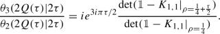
Due to the factor \(\frac{\theta _{1}(Q+\rho )\theta _1(Q-\rho )}{\eta (\tau )^2}\) in (1.17) between the isomonodromic tau function \({\mathcal {T}}_{CM}\) and the determinant tau function \({\mathcal {T}}^{(1,1)}\), we have the following statement:
i.e. the zero locus of the Fredholm determinant in \(\rho \) computes the solution to the equation (1.3). This is an isomonodromic version of Krichever’s solution of the isospectral elliptic Calogero–Moser model [26, 27, 35], and justifies the introduction of the extra parameter \(\rho \).
Further comments are in order:
-
1.
We see that, in contrast to the spherical case, now there are two different tau functions, \({\mathcal {T}}_{CM}\) and \({\mathcal {T}}^{(1,1)}\). It is usually supposed that the object called ’tau function’ is related to free fermions, has a determinant representation, and satisfies some bilinear relations. It turns out that only \({\mathcal {T}}^{(1,1)}\) has such properties, in particular, it was shown in [36] that equation (1.3) is equivalent to some bilinear relations on the two \(\rho \)-independent parts of \({\mathcal {T}}^{(1,1)}\). These bilinear relations are the consequences of the blow-up relations for the theory with adjoint matter (for other examples of such equations see [37]). The free-fermionic nature of \({\mathcal {T}}^{(1,1)}\) was shown in [26]. Instead, \({\mathcal {T}}_{CM}\) has one property, which \({\mathcal {T}}^{(1,1)}\) does not have: its derivative gives the Hamiltonian.
-
2.
A consequence of the determinant expression (1.17) for \({\mathcal {T}}_{CM}\) is the following relation between the solution Q to the nonautonomous elliptic Calogero–Moser equation and the determinant (see equations 3.56 and F.3, [26]):
 (2.84)

3 Generalization to the n-Punctured Torus
We now generalize the discussion of the previous section to the GL(N) linear system (1.21) on a torus with n punctures, using the expressions derived in [25] for the matrices \(L,M_{z_k},M_{\tau }\). In this case the matrix elements \(L_{ij}\) of the Lax matrix L(z) are
while the matrix elements of the M-matrices (1.21) are
where the functions \(x(u,z),\, y(u,z)\) are defined in (1.9). The dynamical variablesFootnote 5\(Q_1,\dots ,Q_N\), \(P_1,\dots ,P_N\) satisfy \(\sum _iQ_i=\sum _iP_i=0\) and are canonically conjugated, and the matrices \(S^{(k)}\) satisfy the Kirillov-Kostant Poisson bracket
where we defined \(S^{(k)}:=S^{(k)}_at^a\) in terms of a set of generators \(t_a\) of \(\mathfrak {sl}_N\), and \(f{_{ab}}^{c}\) are the \(\mathfrak {sl}_N\) structure constants. The residues take value in \(\mathfrak {gl}(N)\) due to the U(1) factors \(\Lambda _{k}\).
Notation 2
Given an N-tuple of parameters \((\xi _1,\dots \xi _N)\), and a function \(g(\xi _i)\), \(i=1,\dots ,N\) of these parameters, we define
In particular, when \(g(\xi _i)=\xi _i\), this is
Remark 3
The generic isomonodromic problem on genus one surfaces is formulated in [25] under the requirement that the matrices \(S^{(k)}\), parametrizing the \(\mathfrak {sl}_N\) residues at the punctures \(z_k\), satisfy
For consistency of the construction, (3.7) will be imposed on the \(\mathfrak {sl}_N\) component of the residues, \(S^{(k)}\).
The matrices \(L,M_{z_k},M_{\tau }\) are not single-valued on the torus, but rather under the shift \(z\rightarrow z+\tau \) behave as (using notation 2)
so that the solution of the linear system (1.8) will transform as follows:
where \(M_B\in SL(N)\). The pants decomposition corresponding to the n-punctured torus consists of n trinions, as shown in Fig. 4, with each trinion \({\mathscr {T}}^{[k]}\) associated to its own three-point problem.
where
for \(k =1, \dots n\). As in the 1-point case, we choose \(\widetilde{{\mathcal {Y}}}^{[k]}(z)\) in such a way that
is regular and single-valued around \(z=z_k\) and has no monodromies around two closest A-cycles.

Pants decomposition for the n-punctured torus
In (3.12) we introduced a U(1) parameter \(\Lambda _0\) shifting the monodromy exponent \(\varvec{\sigma }_1\) around \({\mathcal {C}}_{in}^{[1]}\), whose significance will become apparent in Sects. 4.2 and 4.3Footnote 6. The monodromy exponents \(\varvec{m}_k\), \(\varvec{a}_k\) parametrize the SL(N) component of the monodromy, and the \(\varvec{a}_k\)’s satisfy \(\varvec{a}_{n+1} = \varvec{a}_{1}\). In terms of the original problem on the torus, the monodromy exponents \(\varvec{\sigma }_{k}\), \(\varvec{\mu }_{k}\) in equation (3.10) are defined by the conjugacy class of the monodromies around the punctures \(\left\{ z_k\right\} _{k=1}^{n}\), and around the circles \({\mathcal {C}}_{in}\), \({\mathcal {C}}_{out}\) being glued in the pants decomposition (see Fig. 4), which are respectively
for \(k= 1,\dots n \), and
The matrix \(G_k\) is the matrix that diagonalizes \(M_{{\mathcal {C}}_{in}^{[k]}}=M_{{\mathcal {C}}_{out}}^{[k-1]}\), while \(G_{n+1}:=M_B\) is the matrix that diagonalizes \(M_{{\mathcal {C}}_{out}}^{[n]}\) as in the one-punctured case, and we fixed \(G_1=\mathbb {1}\). The total Hilbert space \({\mathcal {H}}\) is decomposed into a direct sum of spaces \({\mathcal {H}}^{[k]}\) corresponding to each pair of pants:
where
Definition 6
Corresponding to the solutions \({\mathcal {Y}}(z)\), \(\widetilde{{\mathcal {Y}}}^{[k]}(z)\) of the linear problems (1.21), (3.10) respectively, we define two matrix-valued functions: Y(z) with diagonal monodromies around the boundary circles \({\mathcal {C}}^{[k]}_{in}\) and \({\mathcal {C}}^{[k]}_{out}\), and \({\widetilde{Y}}^{[k]}(z)\) with diagonal monodromies around \({\mathcal {C}}^{[k]}_{in}\) and \({\mathcal {C}}^{[k]}_{out}\) (see Fig. 4), by the following equations:
with \(G_{1}= \mathbb {1}\), and \(G_{n+1}= M_{B}\).
The functions \(f^{[k]}(z) \in {\mathcal {H}}^{[k]}\) are decomposed as
The generalization of Definition 4 to the n-punctured case is as follows:
where \({\mathcal {P}}^{[k]}\) is the Plemelj operator given by the solution to the three-point problem (3.10) in the pants decomposition,
Equivalently,
where
The functions \({\widetilde{Y}}_{in}^{[k]},{\widetilde{Y}}_{out}^{[k]}\) are the local solutions of the k-th three-point problem around \({\mp } i\infty \), respectively, defined in Definition 6. In the case of a semi-degenerate system (i.e. a linear system with a single independent local monodromy exponent at \(z=0\) instead of N) these solutions are described by generalized hypergeometric functions \(_NF_{N-1}\) (see eq. 19 in [38]). Similar to (2.20), \( {\mathcal {P}}_{\oplus }^2 = {\mathcal {P}}_{\oplus }\), and
Generalizing Definition 2, we now introduce the Plemelj operator described by the solution to the n-point linear system (1.21),
where
and
where
and as before \(\rho \) is an arbitrary parameter, and \(\Xi _N\) transforms as
The shift of the parameter \(\rho \) in (3.29) makes the monodromies of the Cauchy kernel time-independent (see equation (3.9)), and the following is true:
where \({\mathscr {A}}:= \bigcup _{k=1}^{n} {\mathscr {A}}^{[k]}\) in Fig. 4, and the space of functions are defined by the equation (3.45). It is straightforward to check that \( {\mathcal {P}}_{\Sigma _{1,n}}^2 = {\mathcal {P}}_{\Sigma _{1,n}}\), and one can further prove:
The space of functions on \({\mathscr {T}}:=\bigcup _{k=1}^{n} {\mathscr {T}}^{[k]}\) in Fig. 4 is
Definition 7
The determinant tau function \({\mathcal {T}}^{(1,n)}\) is defined in terms of the Plemelj operators in equations (3.21), (3.26), as
We now proceed to formulate the generalization of proposition 1 to the present case.
3.1 Block-determinant representation of the tau function
Proposition 2
The tau function \({\mathcal {T}}^{(1,n)}\) in (3.34) is the Fredholm determinant of a block operator acting on \(L^{2}(S^{1}) \otimes \left( \bigoplus _{k=1}^{2n} {\mathbb {C}}^N \right) \):
where

and
The operators \({\textsf {a}}^{[k]}, {\textsf {b}}^{[k]}, {\textsf {c}}^{[k]}, {\textsf {d}}^{[k]}\) defined in (3.24), and \(\nabla \) is the shift operator defined in (3.41).
Proof
The proof goes along the same lines as that of Proposition 1. Recalling the definition of the tau function in (3.34) and of the Plemelj operators in (3.22), (3.26), we compute the action of \({\mathcal {P}}_{\Sigma _{1,n},+}^{-1} {\mathcal {P}}_{\oplus ,+}\) on a function \(f\in {\mathcal {H}}_{+}\):
Now we use that for any projector \(\mathcal P\) acting on a vector x, one has \(x-\mathcal P x\in \text {ker } \mathcal P\), and thatFootnote 7\( \text {ker } {\mathcal {P}}_{\Sigma _{1,n}}={\mathcal {H}}_{\mathscr {A}}\):
The orthogonal decomposition of A is
The z-dependent B-cycle monodromy in (3.9) implies that the monodromies around \({\mathcal {C}}_{in}^{[1]}\) and \({\mathcal {C}}_{out}^{[n]}\) (see Fig. 4) are given by (3.14), prompting the following expression for the shift operator \(\nabla :{\mathcal {H}}^{[1]}_{in} \rightarrow {\mathcal {H}}^{[n]}_{out}\)
in order to ’glue’ the boundary spaces on \({\mathcal {C}}_{in}\), \({\mathcal {C}}_{out}\). The factor \(e^{2\pi i z \sum _{j=1}^{n} \Lambda _{j}}\) in the above definition of \(\nabla \) leads to the following action of \(\nabla ^{-1}\):
Identifying the boundaries \({\mathcal {C}}^{[n]}_{out}\) with \({\mathcal {C}}^{[1]}_{in}\), and \({\mathcal {C}}^{[k]}_{out}\) with \({\mathcal {C}}^{[k+1]}_{in}\) for \(k = 1\ldots n-1\), produces the torus from the pants decomposition as in Fig. 4, and translates to the following constraints on A in (3.40):
where the translation operator \(\nabla :{\mathcal {H}}^{[1]}_{in}\rightarrow {\mathcal {H}}^{[n]}_{out}\) is defined as in (3.41). Component-wise, equation (3.39) reads
Imposing the condition that the \({\mathcal {H}}_{-}\) component of F is zero, and using the constraints in (3.43) we get
Substituting (3.45) in (3.44),
Similar to (2.41), we conjugate \({\widehat{K}}_{1,n}\) with the diagonal operator \(\mathrm{\text {diag}}\left( 1,1,\ldots ,\nabla ^{-1} \right) \)
obtaining equation (3.36). \(\square \)
Remark 4
It is straightforward to recover (2.29) from the kernel below.

Kernel
Moreover, the block form of the tau function \({\mathcal {T}}^{(1,n)}\) includes naturally an \((n-1)\times (n-1)\) sub-block identical to the tau function appearing in pg. 18 of [5] for the \(n+2\)-punctured sphere, as emphasised in Fig. 5. This is a consequence of the fact that if we cut the tube that joins the first and last trinion in Fig. 4, (i.e. if we take the limit \(\tau \rightarrow +i\infty \)), we obtain a Fuchsian problem for an \(n+2\)-punctured sphere:
3.2 Relation to the Hamiltonians
Theorem 2
The isomonodromic tau function \({\mathcal {T}}_{H}\) in (1.22) is related to the Fredholm determinant of the operator \(K_{1,n}\) in (3.36) as
where \(\Upsilon _{1,n}\) is an arbitrary function of the monodromy data of the linear system (1.21), \(Q_{i} \equiv Q_{i}(\tau , z_{1},\ldots ,z_{n})\) are the Calogero-like dynamical variables in the linear system (3.1), \( \varvec{\sigma }_{k}=\varvec{a}_k+\sum _{j<k}\Lambda _{j}\) are the monodromy exponents defined in (3.13), and \(\varvec{a}_{n+1}=\varvec{a}_1\),
and \(\rho \) is an arbitrary parameter.
Proof
Let us recall equation (3.34):
where the operators \({\mathcal {P}}_{\oplus }\), \({\mathcal {P}}_{\Sigma _{1,n}}\) are defined in (3.22) and (3.26) respectively. The logarithmic derivative of the tau function \({\mathcal {T}}^{(1,n)}\), has two main components: the derivatives with respect to the modular parameter \(\tau \), and the position of the singularities \(\lbrace z_{k}\rbrace _{k=1}^{n}\):
Computation of this derivative can be done exactly in the same way as in [5, page 20]:
The computation for the first term in (3.53) is the same as in the proof for Theorem 1 in Sect. 2.3: the \(\tau \)-derivative is given by
where
Note that the contours of \(I_{z}\), \(I_{w}\) involve only the final trinion, because the identification \(z\sim z+\tau \) glues \(\mathcal C_{out}^{[n]}\) to \(\mathcal C_{in}^{[1]}\), as in Fig. 4. Like in the case of one puncture, \(I_\tau =\sum _lI_\tau ^{(l)}\) vanishes because \(M_\tau \) in (3.3) has zero residue at the punctures, while \(I_w\) vanishes because the z-loop is contractible. Using the notation 2,
we are then left with the following expression (see (2.64) for comparison) for the first term in (3.53):
In the last line we used
so that
Let us now compute the second term in (3.53):
where
since the z-loop is contractible, and
since \(\partial _{z_k}\Xi _N(w,z)\) is regular in \(w \sim z\). The term \(I_{z_{k}}^{(l,3)}\) is computed by expanding \(\Xi _{N}\) for \(w\sim z\) as in (3.28), and using (2.19):
Note that (3.63) can be different from zero only for \(l=k\), because the integrand is regular for \(l\ne k\). To compute the first and second term, we use the regular parts \(L(z)_{reg}\) and \(L_{3pt}^{[k]}(z)_{reg}\) of L(z) (eq. (3.1)) and \(L_{3pt}^{[k]}\) (eq. (3.10)), as well as the explicit expression (3.2): for \(M_{z_k}\):
where we used the identity
To compute the second term in (3.63), we note that \(M_{z_k}\) in (3.2) is simply the singular part at \(z_k\) of L in (3.1) with a negative sign, so that
The last term in (3.63):
since \({\text {tr}}S^{(k)} =0\). To simplify (3.67) further, let us first substitute (3.1), (3.2) in (3.66):
which implies, together with the canonical Poisson bracket \(\{Q_i,P_j\}=\delta _{ij}\), that
Then (3.67) becomes
Substituting (3.64), (3.66), (3.70) back in (3.63),
Putting it all together (3.53):
Integrating (3.72) and substituting (3.29), we obtain (3.49). \(\square \)
4 Charged Partitions and Nekrasov Functions
In this section, we expand the Fredholm determinant (3.35) in terms of its principal minors labeled by random partitions, and show that the resulting combinatorial expression takes the form of a Fourier series of Nekrasov functions, known as dual Nekrasov–Okounkov partition function [8] in the self-dual Omega-background, for a class of four-dimensional \({\mathcal {N}}=2\) supersymmetric gauge theories called circular quiver gauge theories. These are gauge theories with multiple SU(N) gauge groups, each of which is coupled to two matter hypermultiplets in the bifundamental representation, and their partition functions are equal to free fermion conformal blocks on the torus.
4.1 Minor expansion
The Hilbert space \(L^2(S^1)\) admits a natural orthonormal basis of Fourier modes. We now compute the minor expansion of the Fredholm determinant (3.35) in this particular basis. The kernels of the operators \({\textsf {a}}^{[k]},{\textsf {b}}^{[k]},{\textsf {c}}^{[k]},{\textsf {d}}^{[k]}\) in (3.24) read:
Since the solution \({\widetilde{Y}}^{[k]}\) to the k-th three-point problem defined in (3.10) is multivalued on \({\mathcal {C}}_{in},{\mathcal {C}}_{out}\), with monodromy determined by \(\varvec{\sigma }_{k},\varvec{\sigma }_{k+1}\) respectively as in equation (3.13), the matrix elements of the kernels in (4.1) have the following (twisted) Fourier series representation:
with \(\alpha ,\beta =1,\dots ,N\), and \({\mathbb {Z}}'_+\) denoting the set of positive half-integers. The Fourier coefficients \({\textsf {a}}^{-r;\alpha }_{s;\beta },{\textsf {b}}^{-r;\alpha }_{-s;\beta },{\textsf {c}}^{r;\alpha }_{s;\beta },{\textsf {d}}^{r;\alpha }_{-s;\beta }\) were computed in [5], but we will not need their explicit form. A submatrix of either \({\textsf {a}}^{[k]},{\textsf {b}}^{[k]},{\textsf {c}}^{[k]},{\textsf {d}}^{[k]} \), of size \(i\times j\), is denoted by two unordered sets \(\{(r,\alpha )_1,\dots ,(r,\alpha )_i\} \in 2^{{\mathbb {Z}}'_{+} \times \lbrace 1,\ldots ,N \rbrace }\) and \(\{(s,\beta )_1,\dots ,(s,\beta )_j\} \in 2^{{\mathbb {Z}}'_{+} \times \lbrace 1,\ldots ,N \rbrace }\) where r, s are the Fourier indices in the expansion (4.2), and \(\alpha ,\beta \) are the matrix ("color") indices. Such sets comprised of positive (negative) Fourier modes will be denoted by I (J). Minors of K will then be denoted by collections of such sets \({I}:=\{I_1,\dots ,I_n\} \), \({J}:=\{J_1,\dots ,J_n\}\), and a generic minor \(K_{{I},{J}}\) has the form:
A combinatorial interpretation in terms of Maya diagrams and charged partitions proves vital in expressing the minors as Nekrasov functions: the multi-indices (I, J) can be viewed as the positions \(\textsf {h}(m^{(\alpha )})\) and \(\textsf {p}(m^{(\alpha )})\) of ’holes’ and ’particles’ respectively, of a coloured Maya diagram \(\textsf {m}^{(\alpha )}\), where \(\alpha =1,\ldots ,N\), see Fig. 6. Each particle (hole) carries a positive (negative) unit charge, so that the total charge associated to every Maya diagram is
Using the notation
the total charge is
and it is the same for every N-tuple of coloured Maya diagrams appearing in our expansions. Each Maya diagram determines uniquely a charged Young diagram \(\left( \textsf {Y},\textsf {Q}\right) \) as exemplified in Fig. 6. Consequently, the minors can be labeled by N-tuples of charged partitions \(\left( {{\textsf {Y}}},{{\textsf {Q}}}\right) \).
Definition 8
With the labels in terms of partitions \(\textsf {Y}\) and charges \(\textsf {Q}\), let us define the trinion partition function by the following expression:
where \(k=1,\dots , n\), and \(I_{n+1}= I_{1}, J_{n+1}=J_{1}\). \({\mathscr {T}}^{[k]}\) is the k-th trinion in the pants decomposition in Fig. 4.

Young and Maya diagrams
Note that the determinant in (4.7) is non zero for \(\vert I_{k+1} \vert + \vert J_{k} \vert = \vert I_{k} \vert + \vert J_{k+1} \vert \), which in turn implies that all the Maya diagrams carry the same charge \(\textsf {Q}\).
Proposition 3
The determinant tau function \({\mathcal {T}}^{(1,n)}\) in (3.72) has the following minor expansion in terms of the trinion partition functions in (4.7):
where the \(Z^{{{\textsf {Y}}}_{k},{{\textsf {Q}}}_{k} }_{{{\textsf {Y}}}_{k+1},{{\textsf {Q}}}_{k+1} }({\mathscr {T}}^{[k]})\) is the determinant defined in (4.7), \({\sigma }_1:=\left( \sigma _1^{(1)},\dots ,\sigma _1^{(N)} \right) \)Footnote 8 is the vector of monodromy exponents along the A-cycle of the torus, with modular parameter \(\tau \).
Proof
From (4.3), we can read off the minor expansion of the tau function (3.35) in terms of the trinion partition functions in (4.7):
Additionally, we can write the last factor in (4.9) as follows
In the second line of (4.10), we used the fact that if \(\varvec{\sigma }_1\) is the monodromy exponent on \({\mathcal {C}}_{in}^{[1]}\), then the monodromy exponent on \({\mathcal {C}}_{out}\) is \(\varvec{\sigma }_1-\sum _{j=1}^n\Lambda _j\) Since \(s\in I_{1}\), the hole positions in the corresponding Maya diagram \(\textsf {m}\) are \({\textsf {h}(m)}= \left\{ -s_{1},\ldots ,-s_{k} \right\} \), and since \(r\in J_{1}\), the particle positions are \({\textsf {p}(m)} =\left\{ r_1,\ldots ,r_l \right\} \).

Pictorial proof of (4.11)
To obtain the last line in (4.10), we use the following equalities:
which can be read off from Fig. 7 noting that the r’s and s’s are to the left and right sides of the axis respectively. As an example, in the Fig. 7, \({\textsf {p}(m)}=\left\{ \frac{13}{2}, \frac{9}{2}, \frac{3}{2} \right\} \), \({\textsf {h}(m)}=\left\{ \frac{-3}{2} \right\} \). \(\vert Y \vert \) is the \(\#\)boxes in the Young diagram which in the present example is 12. The charge \(\textsf {Q}(m)=2\). \( \sum r\) is the blue area and \(\sum s\) is the red area in the Fig. 7. Equations (4.9), (4.10) imply (4.8). \(\square \)
Although the determinant tau function \({\mathcal {T}}^{(1,n)}\) in (3.35) admits the expansion (4.8), the trinion partition functions (4.7) are known explicitly in terms of Nekrasov functions only in the case where the Lax matrix residues are of rank-1. We denote the determinant tau function for a generic Fuchsian system on the torus with rank-1 residues,i.e. residues of the form \(\varvec{\mu }_k=\left( \mu _1,0,\dots ,0 \right) \), and monodromy exponents around \({\mathcal {C}}_{in}^{[k]}\) given by \({\widetilde{{\mathcal {T}}}}^{(1,n)}:=\det \left[ \mathbb {1}-{\widetilde{K}}_{1,n} \right] \). Using the expressions for \(Z^{{\textsf {Y}}_{k},{\textsf {Q}}_{k} }_{{\textsf {Y}}_{k+1},{\textsf {Q}}_{k+1} }({\mathscr {T}}^{[k]})\) computed in [5, 17] for the rank-1 case, we obtainFootnote 9
where we set \(z_{0}:=z_{n}\), the Fourier series parameters \({\nu }_i\) were defined in [5, 17] in terms of the normalization of the three-point solution, and we have used introduced the functions
G(x) being the Barnes’ G-function, and
with
In the above equations, \({\sigma },{\mu }\in {\mathbb {C}}^N\), \({{\textsf {Y}}},{\textsf {W}}\in {\mathbb {Y}}^N\), where \(a_{{\textsf {Y}}}(\Box )\) and \(l_{{\textsf {Y}}}(\Box )\) denote respectively the arm and leg length of the box \(\Box \) in the Young diagram \({\textsf {Y}}\), as in Fig. 8.
Remark 5
In (4.12), the expression
is the Nekrasov–Okounkov dual partition function [8] of a circular quiver \({\mathcal {N}}=2\), SU(N) gauge theory. By the AGT correspondence [39], \(Z^D\) is equal to a conformal block of N free fermions on the torus, as in [27]. Consequently, we expect \(Z^D\) in (4.16) to satisfy appropriate bilinear equations, along the lines of [12, 13].

Arm and leg length
Our next goal is to relate the explicit expression (4.12) for the tau function \({\widetilde{{\mathcal {T}}}}^{(1,n)}\) of a linear system on the torus with rank-1 residues, to the tau function \({\mathcal {T}}_H\) of an isomonodromic problem, where the residues are generic and satisfy the constrain (3.7). With the observation that any SL(2) matrix can be reduced to rank-1 by a scalar transformation, we will do this for the cases of the 2-particle nonautonomous Calogero–Moser system and of the elliptic Garnier system, which is the restriction to \(N=2\), \(\Lambda ^{(j)}=0\), \(j=1,\dots ,n\) of the linear system (1.21).
4.2 Reduction to rank-1 residues: the case of 2-particle nonautonomous Calogero–Moser system
With the above considerations in mind, we formulate the tau function of the equation (1.3) in terms of the dual Nekrasov–Okounkov partition function (4.12) for the \({\mathcal {N}}=2^*\) gauge theoryFootnote 10: the Lax matrix \(L_{CM}\) in (1.7) behaves as follows around the puncture \(z=0\)
so that it has rank-2 residue. To make it rank-1, we perform the scalar gauge transformation
after which the Lax matrix and its behavior around the puncture become
As a consequence of (4.18), the monodromies will be dressed by additional scalar factors that we denote by \(g_B(z),g_1\) for the B-cycle and for the monodromy around the puncture respectively. The absence of a factor \(g_A\) for the A-cycle, as well as the expression for \(g_B(z)\), are determined by the periodicity of theta functions:
The z-dependence of the factor \(g_B(z)\) leads to a nontrivial factor \(g_1\) for the monodromy around \(z=0\):
The Hamiltonian tau function \({\widetilde{{\mathcal {T}}}}_{CM}\) associated to the gauge-transformed Lax matrix (4.19) is:
Proposition 4
The tau function (1.17) of the equation (1.3) is related to the tau function (4.23) of the rank-1 Lax matrix in (4.18) as
where m is the monodromy exponent at the puncture and \(\tau \) is the isomonodromic time.
Proof
We begin with the equation (4.23):
To compute the last term in (4.25), consider the following integral over the deformed contour \({\mathcal {C}}_{\varepsilon }\) as in Fig. 9
To obtain the last line we use that
The residue on the left hand side of (4.26) is computed shifting z by \(\tau \) and expanding around 0:
and

Contour of integration
Therefore,
Substituting (4.30) in (4.26), and taking the limit \(\epsilon \rightarrow 0\) we get
Therefore,
having set the integration constant to 1 without any loss of generality. \(\square \)
Theorem 3
The isomonodromic tau function \({\mathcal {T}}_{CM}\) admits the following combinatorial expansion:
where the functions \(Z_{inst}\), \(Z_{pert}\) are defined in (4.14), (4.13) respectively, \({a}=\left( a,-a \right) \), with a the local monodromy exponent around the A-cycle of the torus, m is the monodromy exponent at the puncture \(z=0\), \(\rho \) is an arbitrary parameter, Q is the solution of the equations of motion of the 2-particle nonautonomous Calogero–Moser system (1.3), \({{\textsf {Q}}}\) is the vector of charges (4.5), \({\textsf {Q}}\) is the total U(1) charge (4.6), and \({\widetilde{\Upsilon }}_{1,1}\) is an integration constant depending on monodromy data.
Proof
The linear system (4.19) is the specialisation of (3.1) to the case \(n=1\) (with the puncture at 0), \(N=2\). The corresponding monodromy exponents \({\sigma }_{1}\), \({\sigma }_{2}\), and the U(1) shifts \(\Lambda _{0}\), \(\Lambda _{1}\) in (3.12), and the parameter \({\widetilde{\rho }}\) in (3.29), for the present case are
Theorem 2 then implies that the tau function \({\widetilde{{\mathcal {T}}}}_{CM}\) in (4.24) can be written as a Fredholm determinant of an operator we call \({\widetilde{K}}_{1,1}\) whose minor expansion has an interpretation through Nekrasov functions as in (4.12), of the tau-function in (3.49). Therefore,
\(\square \)
Remark 6
Equation (4.33) coincides with equations (3.48) (4.10) in [26], obtained by CFT methods. To compare the two expressions, one has to set \(\sigma =0\) and send \(\rho +\frac{1}{2}+\frac{\tau }{2}\rightarrow -\rho +\frac{m(\tau +1)}{2}\) in the expressions of [26].
4.3 Elliptic Garnier system and Nekrasov functions
For the \(N\times N\) case, it is in general only possible, with a scalar gauge transformation, to reduce the rank of the residues to \(N-1\), which means that the minors can be written in terms of Nekrasov functions only in the case of semi-degenerate residues, as in [14, 17].Footnote 11 Therefore, we restrict the Lax matrix in (3.1) to \(N=2\), which can always be reduced to rank-1 by the scalar gauge transformation
where \(m_k\) is the local monodromy exponent at the puncture \(z_k\). The new Lax matrix is
The U(1) factors around the punctures are given by
while \(g_A,g_B(z)\), are induced as before by the periodicity of theta functions:
where we defined
Again, we want to find the relation between the isomonodromic tau function \({\mathcal {T}}_H\) of the SL(2) elliptic Garnier system [24, 25, 29], and the GL(2) tau function \({\widetilde{{\mathcal {T}}}}_H\) for the system with rank-1 residues obtained from the scalar gauge transformation (4.37), defined by
Proposition 5
The tau function \({\widetilde{{\mathcal {T}}}}_H\) (4.43) of the rank-1 system is related to the tau function \({\mathcal {T}}_H\) (1.22) of the Garnier system (whose Lax matrix is (3.1) restricted to \(N=2\), \(\Lambda _i=0\) for \(i=1,\dots ,n\)) as
where \(m_k\) is the local monodromy exponent at the puncture \(z_k\), \(k=1,\dots , n\), and \(\tau \) is the modular parameter of the torus.
Proof
Under the transformation (4.37), the \(z_k\)-derivative of \({\widetilde{{\mathcal {T}}}}_H\) is
In the last line we use that
and
We now turn to the computation of the \(\tau \)-derivative:
Let us consider the A-cycle integral of the first term in equation (4.48).

Contour of integration
The computation goes along the same lines of the \(n=1\) case (4.26), but in the present case we do not shift the contour by \(i\epsilon \), since the singularity \(z_l\) is now in the interior of the contour \({\mathcal {C}}\) in Fig. 10:
while
Equating (4.49), (4.50), we see that the first term of (4.48) simply consists of n copies of the 1-point computation (4.31):
We then turn to the computation of the second term of (4.48):
To compute \(I_{kl}\), we consider the following integral over the deformed contour \({\mathcal {C}}\) in Fig. 10:
The left-hand side of (4.53) is
Equating (4.54) and (4.53), we find
Therefore, the second term of (4.48) reads
Substituting (4.51) and (4.56) in (4.48),
Combining (4.45) and (4.57) we find
Integrating the above equation on both sides and setting the integration constant to 1, we obtain
\(\square \)
Remark 7
Note that (4.44) takes the form of the partition function for a Coulomb gas on a torus, with the first term encoding the self-interaction of the particles, while the second term encodes the pairwise interactions.
Using Proposition 5, it is possible to write the tau function of the elliptic Garnier system as a Fourier series of Nekrasov partition functions.
Theorem 4
The isomonodromic tau function of the elliptic Garnier system (see (3.49) restricted to \(N=2\)) admits the following combinatorial expression:
where the functions \(Z_{inst}\), \(Z_{pert}\) are defined in (4.14), (4.13) respectively, \({a}_k=\left( a_k,-a_k \right) \), \(a_k\) being the \(\mathfrak {sl}_2\) local monodromy exponent on the circle \({\mathcal {C}}_{in}^{[k]}\) in Fig. 4, \(m_k\) is the \(\mathfrak {sl}_2\) monodromy exponent at the puncture \(z_k\), \(Q\equiv Q(\tau ; z_{1},\ldots ,z_{n})\) is the Calogero-like variable in the Lax matrix (3.1) specialized to \(N=2\), \(\tau \) is the modular parameter, \({\widetilde{\Upsilon }}_{1,n}\) is an integration constant that depends on the monodromy data, \(({{\textsf {Y}}}, {{\textsf {Q}}})\) are charged partitions,
and \(\rho \) is an arbitrary parameter.
Proof
The Lax matrix (4.38) is the same as (3.1) specialised to n-punctures, \(N=2\). The monodromy exponents \({\sigma }_{k}\), the U(1) shifts \(\Lambda _{k}\) in (3.12), and the parameter \({\widetilde{\rho }}\) defined in (3.29) read as follows for the present case:
with m defined in (4.42), and
Theorem 2 then implies that the tau function \({\widetilde{{\mathcal {T}}}}_{H}\) in (4.44) can be written in terms of a Fredholm determinant of an operator we call \({\widetilde{K}}_{1,n}\) which in turn can be written in terms of Nekrasov functions as in (4.12).
\(\square \)
5 Comments on the Riemann–Hilbert Problem on the Torus and Generalization of the Widom Constant
It is known from [16] that the isomonodromic tau function of a linear system on a sphere can be identified with the so-called Widom constant [42], which depends only on the \(N\times N\) jump matrix \(G(z)\) of the associated Riemann-Hilbert problem (RHP) with unit determinant. For the 4-point isomonodromic problem on a sphere, the general RHP can be recast as a RHP on a unit circle with the jump \(G(z)\) is given by the ratio of the solutions \(\psi _{in,out}\) of the auxiliary 3-point problems:
and admits Birkhoff factorization. Finding the opposite factorization to (5.1) is equivalent to solving the RHP with the above jump condition, which in turn is the same as solving the general 4-point RHP.
Following the same logic, we rewriteFootnote 12 the Fredholm determinant (1.17) in terms of the ratio of the solutions to the 3-point problem \({\widetilde{Y}}\) as defined in (2.1), and the projectors \(\Pi _{\pm }\) onto \({\mathcal {H}}^0_{\pm }\), where \({\mathcal {H}}^0_{\pm }\) are spaces of functions with identical A-cycle monodromies (in this section “\(+\)” and “−” are understood in the sense of (2.12)):
where we set
Using the fact that \(\Pi _{\mp }\) vanishes on \({\mathcal {H}}_\pm ^0\), and conjugating (5.2) by the matrix \({\text {diag}}\left( {\widetilde{Y}}_-^{-1},{\widetilde{Y}}_+^{-1}\right) \), which is an isomorphism \({\mathcal {H}}_-\oplus {\mathcal {H}}_+\rightarrow {\mathcal {H}}^0_-\oplus {\mathcal {H}}^0_+\), we get:
Defining the jump function
and writing \(\nabla \) explicitly as in (2.37), we propose the following definition for a tau function generalizing the Widom constant to the case of the torus.
Definition 9
The torus tau function for the jump J(z) defined in (5.5) is
where
\(\rho \) is an arbitrary parameter, and \(\tau \) is the modular parameter.
Let us now find an appropriate definition of the corresponding RHP. Consider the solution to the the torus one-point linear system \({\mathcal {Y}}(z)\) in (1.7), whose monodromies inside the fundamental domain are the same as the monodromies of the solution to the 3-pt problem \(\widetilde{{\mathcal {Y}}}(z)\). The function
is analytic inside the fundamental domain, and satisfies the following relation on the A-cycle,
where
making it a natural candidate for solution of the RHP. An important observation here is that unlike in the spherical case, on the torus we have an extra diagonal twist \(e^{2\pi i {\varvec{Q}}[J]}\), which implies that \(\Psi (z)\) is not a function, but a section of some non-trivial vector bundle on the torus. So we propose the following
Definition 10
The solution of the RHP \(\Psi (z)\) (5.7) with jump \(J(z)\) on the A-cycle of the torus, is a section of a vector bundle, which is analytic in the fundamental domain and satisfies (5.8) at the boundaries. The complex moduli of the bundle \(Q_i[J]\) are some functionals of \(J\).
We conjecture that the RHP for generic jump \(J(z)\) is solvable, and moreover, that complex moduli of the vector bundle are given by zeroes of \({\mathcal {T}}^{(1,1)}[\rho ,J]\) in \(\rho \) as in (2.83):
It should not be hard to verify that the \(\rho \)-dependence of \({\mathcal {T}}^{(1,1)}[\rho ,J]\) should be factorizable as in the 1-point case (1.17), or even in the more general case (3.49), with the \(\rho \)-independent part that we denote by \({\mathcal {T}}^{(1,1)}_0[J]\):
Furthermore, the solution to the RHP (5.8) is not unique. Namely, if \(\Psi _{N}(z)\) is a solution to the \(N \times N\) RHP, then
where \(\sum _{i=1}^N k_i=0\), is also a solution with the moduli of the vector bundle given by
using the Notation 2. This demonstrates that \(Q_i\)’s are points on the same complex torus over which the RHP is formulated (they are the Tyurin points that parametrize the vector bundle on the torus, as in [43, 44]), and is consistent with (5.11).
The next point of discussion is the distinction between what is called the direct RHP (5.8) and the dual one (5.5). In the spherical case the direct and dual RHPs were identical, and even in the present case it seems that we can rewrite the dual RHP in a similar way, \({\widetilde{Y}}_{out}(z+\tau )=J(z){\widetilde{Y}}_{in}(z)\). However, the important difference with respect to the spherical case is that here, \(\Psi (z)\) is analytic for \(\Im z \in [0,\Im \tau ]\), \({\widetilde{Y}}_{in}(z)\) is analytic for \(\Im z\in (-i\infty ,0]\), and \({\widetilde{Y}}_{out}(z)\) is analytic for \(\Im z\in [\Im \tau ,i\infty )\). So the dual RHP is actually the same Birkhoff factorization problem as in the spherical case, while the direct one is different.
Another interesting question regards the possible options for \(J(z)\). In the 1-puncture case J(z) was constructed from (5.3), where \({\widetilde{Y}}_-\), \({\widetilde{Y}}_+\) were the analytic continuations of the same function in two different regions. We do not know the features of the RHPs with such jumps, which jumps are more natural to consider, and what is the natural \(\tau \)-dependence of \(J(z)\).
In the torus case, the jump \(J(z)\) can be in principle \(\tau \)-dependent, but we can also consider \(\tau \)-independent jump \(J(z)\) and find a limit to the usual Widom constant. Namely, setting \(\rho =\tau /2\), one finds that the eigenvalues of \(e^{-2\pi i\rho +\tau \partial _z}\) acting on \({\mathcal {H}}_-^0\) are \(e^{2\pi i (n+1/2)\tau }\) for \(n\ge 0\), and similarly for \(e^{2\pi i\rho -\tau \partial _z}\) acting on \({\mathcal {H}}_+^0\) (recall the definition of \({\mathcal {H}}_{+}\) in (2.12)). They vanish in the \(\tau \rightarrow i\infty \) limit, so we are left with the standard determinant giving the Widom constant. We also see this degeneration at the level of the RHP (5.8): \(\Psi (z)\) at the boundaries can be first approximated by Fourier series’ decaying towards the interior of the fundamental domain, and then consistency conditions around \(z=\tau /2\) will introduce corrections of order \({\mathcal {O}}\left( e^{\pi i\tau }\right) \).
Another observation is that equation (5.8), for rational \(J(z)\), can be considered as the solution to a \(q\)-difference linear system. In this case \(\varvec{Q}[J]\) has a different interpretation: following the \(q\)-difference generalization of the approach of [45] to difference equations, we introduce the following function
which solves an equation
Then, \(\varvec{Q}[J]\) parametrizes the local monodromy of the \(q\)-difference system, since
and the monodromy matrix \(e^{-2\pi i\varvec{Q}[J]/\tau }\) is defined up to multiplication by \(e^{-2\pi i\varvec{k}/\tau }\), due to the presence of the \(\tau \)-periodic exponentials \(e^{-2\pi i\varvec{k} z/\tau }\).
Another interesting question is then the following: what is the meaning of the torus tau function in this case of the \(q\)-difference system, and what information can we extract about the local monodromy from equation (5.10)? What is the generalization of the Widom formula for the variation of \({\mathcal {T}}^{(1,1)}[\rho ,J]\) under the variations of \(J(z)\)? We leave all these questions for a future work.
6 Outlook and Discussion
An immediate question regards the modular properties of tau functions on the torus which provides a way to study the so-called connection constant [10, 46]. A starting point in analyzing the modular properties of the tau function \({\mathcal {T}}_{H}\) in (3.49) is the free fermion conformal block \(Z^D\) in (4.16), whose transformations can be obtained by using the results of [47,48,49,50,51], where the so-called modular kernel, governing the behavior of the conformal block under modular transformations was derived. The other key ingredient is the variable \(Q_i\) that appears in the argument of the theta functions. Its modular properties have been studied in [20] for the SL(2) one-punctured case, for which Q is the solution of the equation (1.3).
A natural continuation of this work is the generalization of the Fredholm determinant representation of tau functions on higher genus (\(g\ge 2\)) Riemann surfaces, and for \(g\ge 1\) cases with irregular singularities. The main obstacle in providing explicit formulas for the tau function in both these cases is that the corresponding pants decomposition necessarily contains trinions with no external legs (see Fig. 11), for which the construction for the matrix elements of the Plemelj operators is not clear. Solving the problem posed by the all-internal trinion would immediately allow us to generalize several results on the Riemann sphere [15, 16, 52, 53] to the case of the torus.

Pants decomposition for a genus-2 Riemann surface
The explicit formulas for the higher genus case would have important consequences in theoretical physics as well: the relation between the isomonodromic tau function and free fermion conformal blocks argued in [54] would provide new explicit formulas for higher genus conformal blocks. From yet another perspective, the determinant tau functions studied in this paper coincide with partition functions of topological string theory on certain local Calabi-Yau threefolds, as already observed in [26], and the identification with determinants provides a powerful nonperturbative definition of such partition functions [28, 55,56,57,58]. Further extending our construction to higher genus Riemann Surfaces and irregular punctures would provide explicit formulas for cases that have proven inaccessible by usual methods, like the topological vertex [59]. In CFT, these would be given by irregular conformal blocks on Riemann surfaces (for relations of irregular conformal blocks on the sphere with Painlevé equations, see also [38, 60,61,62]).
Notes
The dependence on the variables \(\tau \), \(z_{1},\ldots , z_{n}\) of the functions \({\mathcal {Y}}(z)\), L(z), M(z), \(H_{k}\), \(H_{\tau }\), \({\mathcal {T}}_{H}\) is dropped henceforth for brevity.
Here on, we drop the \(\tau \) dependence of Q for brevity.
When \(\left( \mathbb {1}- K_{1,1}\right) \) is invertible, \({\mathcal {H}}= {\mathcal {H}}_{{\mathscr {T}}} \oplus {\mathcal {H}}_{A}\), and therefore \(\text {ker } {\mathcal {P}}_{\Sigma _{1,1}}={\mathcal {H}}_{\mathscr {A}}\).
We drop the \(\tau \) dependence of \(Y_{CM}\), \(L_{CM}\) and \(M_{CM}\) in this proof for brevity
In the interest of brevity, we omit writing the \(\tau \), \(z_{1}\ldots z_{n}\) dependence of the functions L(z), M(z), Y(z) and the dynamical variables \(Q_{i}\)’s, \(P_{i}\)’s.
From the point of view of the dynamical system, the monodromy exponents on \({\mathcal {C}}_{in}^{[1]}\) have the role of initial conditions, so that it is natural that \(\Lambda _0\) doesn’t appear in the Lax matrix, contrary to \(\Lambda _1,\dots ,\Lambda _N\), which are residues at the punctures.
As in the previous section, when \(\left( \mathbb {1}- K_{1,n}\right) \) is invertible, \({\mathcal {H}}= {\mathcal {H}}_{{\mathscr {T}}} \oplus {\mathcal {H}}_{A}\), and therefore \(\text {ker } {\mathcal {P}}_{\Sigma _{1,n}}={\mathcal {H}}_{\mathscr {A}}\).
Note that here, differently from (3.13) where we collected the monodromy exponents \(\sigma _i^{(1)},\dots ,\sigma _i^{(N)}\) into diagonal matrices denoted by \(\varvec{\sigma }_i\), we organize them into vectors \({a}_i\), since they are summed with the charges \({{\textsf {Q}}}_i\), that are vectors in the root lattice \({\mathbb {Z}}^N\) of \(\mathfrak {gl}_N\).
Time-independent term \(\frac{1}{2}\sum _{j=1}^{n}\Lambda _j\) comes from the ratios of the asymptotics of \(U(1)\) corrections to solutions of the 3-pt problems, given explicitly by \(\left( \sin \pi (z-z_k)\right) ^{\Lambda _k}\).
This is the SU(2), \({\mathcal {N}}=2\) Super Yang-Mills theory with one massive adjoint hypermultiplet.
In this section, we use the SL(N) analogues of the objects studied in Sect. 2 for the one-punctured torus.
References
Jimbo, M., Miwa, T., Ueno, K.: Monodromy preserving deformations of linear differential equations with rational coefficients. 1. Physica D2, 306 (1981)
Wu, T.T., McCoy, B.M., Tracy, C.A., Barouch, E.: Spin-spin correlation functions for the two-dimensional ising model: exact theory in the scaling region. Phys. Rev. B 13, 316 (1976)
Its, A.R., Izergin, A.G., Korepin, V.E., Slavnov, N.A.: Differential equations for quantum correlation functions. Int. J. Mod. Phys. B 4, 1003 (1990)
Zamolodchikov, A.B.: Painleve III and 2-d polymers. Nucl. Phys. B 432, 427 (1994). arXiv:hep-th/9409108
Gavrylenko, P., Lisovyy, O.: Fredholm determinant and Nekrasov sum representations of isomonodromic tau functions. Commun. Math. Phys. 363, 1 (2018). arXiv:1608.00958
Gavrylenko, P.G., Marshakov, A.V.: Free fermions, W-algebras and isomonodromic deformations. Theor. Math. Phys. 187, 649 (2016). arXiv:1605.04554
Nekrasov, N.A.: Seiberg-Witten prepotential from instanton counting, in International Congress of Mathematicians (ICM 2002) Beijing, China, August 20–28, 2002 (2003). arXiv:hep-th/0306211
Nekrasov, N., Okounkov, A.: Seiberg-Witten theory and random partitions. Prog. Math. 244, 525 (2006). arXiv:hep-th/0306238
Gamayun, O., Iorgov, N., Lisovyy, O.: Conformal field theory of Painlevé VI. JHEP 10, 038 (2012). arXiv:1207.0787
Iorgov, N., Lisovyy, O., Tykhyy, Yu.: Painlevé VI connection problem and monodromy of \(c=1\) conformal blocks. JHEP 12, 029 (2013). arXiv:1308.4092
Iorgov, N., Lisovyy, O., Teschner, J.: Isomonodromic tau-functions from Liouville conformal blocks. Commun. Math. Phys. 336, 671 (2015). arXiv:1401.6104
Bershtein, M., Shchechkin, A.: Bilinear equations on Painlevé \(\tau \) functions from CFT. Commun. Math. Phys. 339, 1021 (2015). arXiv:1406.3008
Bershtein, M.A., Shchechkin, A.I.: Backlund transformation of Painleve III(\(D_8\)) tau function. J. Phys. Series A50, 115205 (2017). arXiv:1608.02568
Gavrylenko, P., Iorgov, N., Lisovyy, O.: Higher rank isomonodromic deformations and \(W\)-algebras. Lett. Math. Phys. 110, 327 (2019). arXiv:1801.09608
Gavrylenko, P., Lisovyy, O.: Pure \(SU(2)\) gauge theory partition function and generalized Bessel kernel. Proc. Symp. Pure Math. 18, 181 (2018). arXiv:1705.01869
Cafasso, M., Gavrylenko, P., Lisovyy, O.: Tau functions as Widom constants. Commun. Math. Phys. 365, 741 (2019). arXiv:1712.08546
Gavrylenko, P., Iorgov, N., Lisovyy, O.: On solutions of the Fuji-Suzuki-Tsuda system. SIGMA 14, 123 (2018). arXiv:1806.08650
Levin, A.M., Olshanetsky, M.A.: Painlevé-Calogero correspondence, pp. 313–332. Springer New York, New York, NY, 2000. https://doi.org/10.1007/978-1-4612-1206-5 20
Takasaki, K.: Painlevé-Calogero correspondence revisited. J. Math. Phys. 42 (2001) 1443 [math/0004118]
Manin, Y.I.: Sixth painlevé equation, universal elliptic curve, and mirror of \(\textbf{P}^2\), arXiv preprint alg-geom/9605010 (1996) arXiv:alg-geom/9605010
Korotkin, D.A., Samtleben, J.A.H.: On the quantization of isomonodromic deformations on the torus. Int. J. Mod. Phys. A 12, 2013 (1997). arXiv:hep-th/9511087
Levin, A., Olshanetsky, M.: Hierarchies of isomonodromic deformations and hitchin systems. Transl. Am. Math. Soc. Ser. 2(191), 223 (1999)
Takasaki, K.: Elliptic Calogero-Moser systems and isomonodromic deformations. J. Math. Phys. 40, 5787 (1999)
Korotkin, D., Manojlovic, N., Samtleben, H.: Schlesinger transformations for elliptic isomonodromic deformations. J. Math. Phys. 41, 3125 (2000). arXiv:solv-int/9910010
Levin, A., Olshanetsky, M., Zotov, A.: Classification of isomonodromy problems on elliptic curves. Russ. Math. Surveys 69, 35 (2014). arXiv:1311.4498
Bonelli, G., Del Monte, F., Gavrylenko, P., Tanzini, A.: \(\cal{N} =2^*\) gauge theory, free fermions on the torus and Painlevé VI. Commun. Math. Phys. 377, 1381 (2020). arXiv:1901.10497
Bonelli, G., Del Monte, F., Gavrylenko, P., Tanzini, A.: Circular quiver gauge theories, isomonodromic deformations and \(W_N\) fermions on the torus. arXiv:1909.07990
Bonelli, G., Grassi, A., Tanzini, A.: Seiberg Witten theory as a Fermi gas. Lett. Math. Phys. 107, 1 (2017). arXiv:1603.01174
Takasaki, K.: Spectral curve and Hamiltonian structure of isomonodromic SU(2) Calogero-Gaudin system. J. Math. Phys. 44, 3979 (2003). arXiv:nlin/0111019
Malgrange, B.: Sur les déformations isomonodromiques. I. Singularités régulières, pp. 1–26. No. 17 in Cours de l’institut Fourier. Institut des Mathématiques Pures-Université Scientifique et Médicale de Grenoble (1982)
Bertola, M.: The dependence on the monodromy data of the isomonodromic tau function. Commun. Math. Phys. 294, 539 (2010). arXiv:0902.4716
Bertola, M.: CORRIGENDUM: The dependence on the monodromy data of the isomonodromic tau function. ArXiv e-prints (2016) arXiv:1601.04790
Hatcher, A.: Pants Decompositions of Surfaces, arXiv Mathematics e-prints (1999). arXiv:math/9906084
Goldman, W.M.: Trace Coordinates on Fricke spaces of some simple hyperbolic surfaces. arXiv e-prints (2009) arXiv:0901.1404
Krichever, I.M.: Elliptic solutions of the Kadomtsev-Petviashvili equation and integrable systems of particles. Funct. Anal. Appl. 14, 282 (1980)
Bershtein, M., Gavrylenko, P., Grassi, A.: to appear
Gu, J., Haghighat, B., Klemm, A., Sun, K., Wang, X.: Elliptic Blowup Equations for 6d SCFTs. III: E-strings, M-strings and Chains. arXiv:1911.11724
Gavrylenko, P., Marshakov, A., Stoyan, A.: Irregular conformal blocks, Painlevé III and the blow-up equations. arXiv:2006.15652
Alday, L.F., Gaiotto, D., Tachikawa, Y.: Liouville correlation functions from four-dimensional Gauge theories. Lett. Math. Phys. 91, 167 (2010). arXiv:0906.3219
Gaiotto, D.: N=2 dualities. JHEP 08, 034 (2012). arXiv:0904.2715
Gaiotto, D., Moore, G.W., Neitzke, A.: Wall-crossing, hitchin systems, and the WKB approximation. arXiv:0907.3987
Widom, H.: Asymptotic behavior of block Toeplitz matrices and determinants. II. Adv. Math. 21, 1 (1976)
Krichever, I.: Vector bundles and Lax equations on algebraic curves. Commun. Math. Phys. 229, 229 (2002). arXiv:hep-th/0108110
Krichever, I.: Isomonodromy equations on algebraic curves, canonical transformations and Whitham equations. arXiv:hep-th/0112096
Krichever, I.: Analytic theory of difference equations with rational and elliptic coefficients and the Riemann–Hilbert problem. Russ. Math. Surveys 59, 1117 (2004). arXiv:math-ph/0407018
Its, A., Lisovyy, O., Tykhyy, Y.: Connection problem for the sine-Gordon/Painlevé III tau function and irregular conformal blocks. arXiv:1403.1235
Ponsot, B., Teschner, J.: Liouville bootstrap via harmonic analysis on a noncompact quantum group. arXiv:hep-th/9911110
Ponsot, B., Teschner, J.: Clebsch–Gordan and Racah–Wigner coefficients for a continuous series of representations of U(q)(sl(2, R)). Commun. Math. Phys. 224, 613 (2001). arXiv:math/0007097
Hadasz, L., Jaskolski, Z., Suchanek, P.: Proving the AGT relation for N_f = 0,1,2 antifundamentals. JHEP 06, 046 (2010). arXiv:1004.1841
Nemkov, N.: On modular transformations of toric conformal blocks. JHEP 10, 039 (2015). arXiv:1504.04360
Nemkov, N.: Analytic properties of the Virasoro modular kernel. Eur. Phys. J. C 77, 368 (2017). arXiv:1610.02000
Desiraju, H.: The \(\tau \)-function of the Ablowitz-Segur family of solutions to Painlevé II as a Widom constant. J. Math. Phys. 60, 113505 (2019). arXiv:1906.11517
Desiraju, H.: Fredholm determinant representation of the Painlevé II \(\tau \)-function, arXiv e-prints (2020). arXiv:2008.01142
Del Monte, F.: Supersymmetric Field Theories and Isomonodromic Deformations. Ph.D. thesis (2020)
Grassi, A., Hatsuda, Y., Marino, M.: Topological strings from quantum mechanics. Annales Henri Poincare 17, 3177 (2016). arXiv:1410.3382
Bonelli, G., Grassi, A., Tanzini, A.: New results in \(\cal{N} =2\) theories from non-perturbative string. Annales Henri Poincare 19, 743 (2018). arXiv:1704.01517
Coman, I., Pomoni, E., Teschner, J.: From quantum curves to topological string partition functions. arXiv:1811.01978
Coman, I., Longhi, P., Teschner, J.: From quantum curves to topological string partition functions II. arXiv:2004.04585
Aganagic, M., Klemm, A., Marino, M., Vafa, C.: The Topological vertex. Commun. Math. Phys. 254, 425 (2005). arXiv:hep-th/0305132
Bonelli, G., Lisovyy, O., Maruyoshi, K., Sciarappa, A., Tanzini, A.:On Painlevé/gauge theory correspondence. arXiv:1612.06235
Nagoya, H.: Irregular conformal blocks, with an application to the fifth and fourth Painlevé equations. J. Math. Phys. 56, 123505 (2015). arXiv:1505.02398
Nagoya, H.: Remarks on irregular conformal blocks and Painlevé III and II tau functions. arXiv e-prints (2018) arXiv:1804.04782
Acknowledgements
We thank G. Bonelli, T. Grava, O. Lisovyy, A. Tanzini for their useful comments. Thanks are also due to the organizers of the workshops Geometric Correspondences of Gauge Theories (Trieste 2019) and Winter School on Integrable Systems and Representation Theory (Bologna, 2020) for their hospitality. F.D.M. thanks SISSA for providing him support in this taxing time after the end of his PhD. The work of P.G. is partially supported by the HSE University Basic Research Program, Russian Academic Excellence Project ’5-100’ and by the RSF Grant No. 19-11-00275 (results of Sects. 2.1 and 5 were funded by RSF). The work of H.D is partly supported by H2020-MSCA-RISE-2017 PROJECT No. 778010 IPaDEGAN. H.D thanks INFN Iniziativa Specifica GAST, and F.D.M thanks INFN Iniziativa Specifica ST &FI, for funding the travel to Winter School on Integrable Systems and Representation Theory (Bologna, 2020) where a part of the work was done. The work of F.D.M. was funded by SISSA, under the project "Fredholm determinants for tau functions and supersymmetric partition functions". A special thanks to the apps Microsoft Whiteboard, Telegram, and Zoom, where most of the work was done. P.G. would also like to thank Emacs+CDLaTeX+Magit.
Funding
Open Access funding enabled and organized by CAUL and its Member Institutions.
Author information
Authors and Affiliations
Corresponding author
Additional information
Communicated by J-d.Gier.
Publisher's Note
Springer Nature remains neutral with regard to jurisdictional claims in published maps and institutional affiliations.
Rights and permissions
Open Access This article is licensed under a Creative Commons Attribution 4.0 International License, which permits use, sharing, adaptation, distribution and reproduction in any medium or format, as long as you give appropriate credit to the original author(s) and the source, provide a link to the Creative Commons licence, and indicate if changes were made. The images or other third party material in this article are included in the article’s Creative Commons licence, unless indicated otherwise in a credit line to the material. If material is not included in the article’s Creative Commons licence and your intended use is not permitted by statutory regulation or exceeds the permitted use, you will need to obtain permission directly from the copyright holder. To view a copy of this licence, visit http://creativecommons.org/licenses/by/4.0/.
About this article

Cite this article
Del Monte, F., Desiraju, H. & Gavrylenko, P. Isomonodromic Tau Functions on a Torus as Fredholm Determinants, and Charged Partitions. Commun. Math. Phys. 398, 1029–1084 (2023). https://doi.org/10.1007/s00220-022-04458-y
Received:
Accepted:
Published:
Issue Date:
DOI: https://doi.org/10.1007/s00220-022-04458-y