Amplitudes in YM and GR as a Minimal Model and Recursive Characterization

Abstract

We study the tree scattering amplitudes of Yang–Mills and General Relativity as functions of complex momenta, using a homological and geometrical approach. This approach uses differential graded Lie algebras, one for YM and one for GR, whose Maurer Cartan equations are the classical field equations. The tree amplitudes are obtained as the $L_\infty$ minimal model brackets, given by a trivalent Feynman tree expansion. We show that they are sections of a sheaf on the complex variety of momenta, and that their residues factor in a characteristic way. This requires classifying the irreducible codimension one subvarieties where poles occur; constructing dedicated gauges that make the factorization manifest; and proving a flexible version of gauge independence to be able to work with different gauges. The residue factorization yields a simple recursive characterization of the tree amplitudes of YM and GR, by exploiting Hartogs’ phenomenon for singular varieties. This is similar to and inspired by Britto–Cachazo–Feng–Witten recursion, but avoids BCFW’s trick of shifting momenta, hence avoids conditions at infinity under such shifts.

1 Introduction

Gauge theories in physics are redundant in their description of physical processes; to extract actual physical information one must quotient by a large gauge group. Tree scattering amplitudes in Yang–Mills theory (YM) and General Relativity (GR) are interesting because they are gauge independent. They are extensively studied in the physics literature, see for example the Parke–Taylor formulas for YM amplitudes in [1, 2] exposing significant cancellations among Feynman graphs for certain helicity configurations;¹ the discussion of the factorization of residues along collinear and multiparticle singularities in [2] and earlier S-matrix literature; the Britto–Cachazo–Feng–Witten (BCFW) recursion relations in [3, 4]; the monograph [5] and a textbook [6].

Amplitudes are naturally studied on complex momentum space, e.g. [3]. The significance is clear already for 3-point amplitudes: Both for YM and GR, the 3-point amplitudes vanish identically for real momenta, but they do not vanish for complex momenta. This is paradoxical, since vanishing on the real points often implies vanishing in the complex.² The paradox is resolved by noting that the complex algebraic variety on which the 3-point amplitudes live has two irreducible components; these two components are conjugate to each other; hence the real points are contained in the intersection of the two irreducible components; hence the real points are not Zariski dense.

Summary. This paper concerns the ordinary, physical tree amplitudes of YM and GR, as functions of complex momenta. In our approach, they arise as $L_\infty$ minimal model brackets using trivalent (cubic) Feynman tree graphs. We then study their recursive characterization independent of Feynman graphs, based on factorization. This paper includes details often taken for granted in the literature on amplitudes, and departs conceptually from it because the development is consistently homological and geometrical.

The relation between homotopy minimal models and scattering amplitudes in another context, string field theory, is discussed in [7]. A systematic algebraic account of minimal models and homotopy transfer is in [8].

We treat YM and GR in a uniform way, by formulating each as a differential graded Lie algebra, based on [9,10,11,12]. These dgLa carry a grading by complex momentum $k \in \mathbbm {C}^4$. Their homology ${{{\mathfrak {h}}}}_k$ is nonzero only when k is on the complex light cone. The tree amplitudes are then the $L_\infty$ minimal model brackets $\{-,\dots ,-\}: {{{\mathfrak {h}}}}_{k_1}^1 \otimes \cdots \otimes {{{\mathfrak {h}}}}_{k_n}^1\rightarrow {{{\mathfrak {h}}}}_{k_1+\dots +k_n}^2$ of these dgLa, given by a sum of trivalent Feynman tree graphs. Our main results are:

• We give a homological proof of gauge independence, required to show that the amplitudes are well-defined. The point of this theorem (Theorem 5) is that its assumptions are weak: any gauge, namely any momentum conserving contraction used in the Feynman tree graphs, gives identical amplitudes $\{-,\ldots ,-\}$. We exploit this flexibility in the rest of the paper.

• We show that the YM and GR amplitudes are sections of a sheaf on the variety of kinematically admissible complex momenta (Theorem 12) and satisfy the key residue factorization of the caricatural form (Theorem 14)

  $$\begin{aligned} {{\,\mathrm{Res}\,}}_{{\mathfrak {p}}}\{\ldots \} \;=\; \{\ldots ,\{\ldots \}\} \end{aligned}$$

  (1)

  To make sense of this, we must classify all prime divisors ${{\mathfrak {p}}}$ corresponding to the irreducible codimension one subvarieties along which the amplitudes can have poles (Theorem 9). Our main tool to prove (1) are dedicated gauges, that we call optimal homotopies, and that we construct in a general setting using the homological perturbation lemma (Theorem 8).

• We prove that (1) determine the amplitudes uniquely, among all sections satisfying some obvious conditions such as their homogeneity degree. This recursive characterization (Theorem 13) is similar to and inspired by [3], but avoids BCFW’s characteristic trick of deforming momenta, resulting in a characterization with weaker assumptions. It is based on a conceptually more straightforward Hartogs extension property (Theorem 10).

Extended summary. For YM respectively GR about Minkowski spacetime we use a dgLa ${{\mathfrak {g}}}$ whose Maurer–Cartan equation

$$\begin{aligned} du + \tfrac{1}{2} [u,u] \;=\; 0 \end{aligned}$$

(2)

with unknown $u \in {{\mathfrak {g}}}^1$, is equivalent to the classical partial differential field equation. Here $d: {{\mathfrak {g}}}^1 \rightarrow {{\mathfrak {g}}}^2$ is the differential and $[-,-]: {{\mathfrak {g}}}^1 \otimes {{\mathfrak {g}}}^1 \rightarrow {{\mathfrak {g}}}^2$ is the bracket. The Lie algebra ${{\mathfrak {g}}}^0$ implements gauge transformations. We use ${{\mathfrak {g}}}$ to construct the tree amplitudes that are ordinarily constructed using an action, namely the YM respectively Einstein–Hilbert Lagrangian. Briefly:³

• For YM, the complex underlying ${{\mathfrak {g}}}$ has the following form [9,10,11]:

  

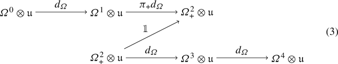
  The four columns correspond to the decomposition ${{\mathfrak {g}}}= {{\mathfrak {g}}}^0 \oplus {{\mathfrak {g}}}^1 \oplus {{\mathfrak {g}}}^2 \oplus {{\mathfrak {g}}}^3$. Here $\otimes = \otimes _{\mathbbm {C}}$; $\varOmega = \varOmega (\mathbbm {R}^4)$ are the complex de Rham differential forms; $\varOmega ^2 = \varOmega ^2_+ \oplus \varOmega ^2_-$ is the decomposition into eigenspaces of the Hodge star operator for the Minkowski metric; $\pi _+: \varOmega ^2 \rightarrow \varOmega ^2_+$ is the projection; $d_\varOmega$ is the de Rham differential and in (3) is also an abbreviation for $d_\varOmega \otimes \mathbbm {1}$; and ${{\mathfrak {u}}}$ is any finite-dimensional ‘internal’ or ‘color’ Lie algebra. The gLa bracket ${{\mathfrak {g}}}^i \otimes {{\mathfrak {g}}}^j \rightarrow {{\mathfrak {g}}}^{i+j}$, not detailed in this introduction, only involves the wedge product on $\varOmega$ and the Lie bracket on ${{\mathfrak {u}}}$, hence it is $C^\infty$-bilinear. One can define a formal invariant bilinear pairing on (3) that in particular gives an action [10, 11], but we will not invoke this pairing.

• For GR, the Maurer–Cartan equation (2) is an orthonormal frame formulation of the vacuum Einstein equations [12]; its solutions are the Ricci-flat metrics. The complex underlying ${{\mathfrak {g}}}={{\mathfrak {g}}}^0\oplus {{\mathfrak {g}}}^1\oplus {{\mathfrak {g}}}^2\oplus {{\mathfrak {g}}}^3\oplus {{\mathfrak {g}}}^4$ has the form

  

  Here ${{\mathfrak {v}}}$ is a 10-dimensional Lie algebra; $\varOmega \otimes {{\mathfrak {v}}}$ is a dgLa; and $I=I^2\oplus I^3\oplus I^4$ is a dgLa ideal necessary to obtain GR. The bracket in $\varOmega \otimes {{\mathfrak {v}}}$ is given by a base change formula, see (25), and the differential is $[m,-]$ with m a degree one element that satisfies $[m,m]=0$ and represents Minkowski spacetime. Set ${{\mathfrak {g}}}=(\varOmega \otimes {{\mathfrak {v}}})/I$. The Maurer–Cartan equation (2) has a concrete meaning: The unknown $u \in \varOmega ^1 \otimes {{\mathfrak {v}}}$ is an orthonormal frame and a metric-compatible affine connection; and the vanishing of $du + \tfrac{1}{2} [u,u] \in (\varOmega ^2 \otimes {{\mathfrak {v}}})/I^2$ forces torsion and Ricci curvature of u to vanish but, and this is the role of $I^2$, allows arbitrary Weyl curvature.⁴ While we are not aware of an associated action principle, this dgLa ${{\mathfrak {g}}}$ yields the ordinary GR tree amplitudes.

To construct amplitudes, we restrict to the sub-dgLa of ${{\mathfrak {g}}}$ given by all finite linear combinations of plane waves with complex momenta $k \in \mathbbm {C}^4$. Abusing notation, we now let ${{\mathfrak {g}}}$ be this sub-dgLa.⁵ Denote by ${{\mathfrak {g}}}_k$ the subspace of plane waves with momentum k. Both differential and bracket preserve momentum:

$$\begin{aligned} {{\mathfrak {g}}}= \textstyle \bigoplus _{k\in \mathbbm {C}^4}{{\mathfrak {g}}}_k \qquad \qquad d{{\mathfrak {g}}}_k \subseteq {{\mathfrak {g}}}_k \qquad \qquad [{{\mathfrak {g}}}_{k_1},{{\mathfrak {g}}}_{k_2}]\subseteq {{\mathfrak {g}}}_{k_1+k_2} \end{aligned}$$

Each ${{\mathfrak {g}}}_k$ is a copy of a fixed finite-dimensional graded $\mathbbm {C}$-vector space. Relative to any basis of that vector space, the differential respectively bracket are given by arrays whose entries are first order polynomials in k respectively $k_1$ and $k_2$. As Fourier multipliers, they are first order partial differential operators.

Let ${{{\mathfrak {h}}}}_k = H({{\mathfrak {g}}}_k)$ be the homology of d restricted to ${{\mathfrak {g}}}_k$. Let ${Q}$ be the Minkowski square of k. Then the homology is supported on the complex light cone ${Q}=0$, meaning $H({{\mathfrak {g}}}) = \bigoplus _{k:{Q}=0}{{{\mathfrak {h}}}}_k$. For $k \ne 0$ on the complex light cone:

• The homology ${{{\mathfrak {h}}}}_k$ is concentrated in degrees $i=1,2$.

• Canonically ${{{\mathfrak {h}}}}_k^i = {{{\mathfrak {h}}}}_k^{i,+}\oplus {{{\mathfrak {h}}}}_k^{i,-}$ with summands called helicities.

• There are canonical isomorphisms ${{{\mathfrak {h}}}}_k^{1,\pm } \simeq {{{\mathfrak {h}}}}_k^{2,\pm }$ and⁶${{\,\mathrm{Hom}\,}}_{\mathbbm {C}}({{{\mathfrak {h}}}}_k^{i,\pm },\mathbbm {C}) \simeq {{{\mathfrak {h}}}}_{-k}^{i,\mp }$.

The ${{{\mathfrak {h}}}}_k^{i,\pm }$ are fibers of a sheaf that distinguishes YM from GR.

We define the tree amplitudes as the $L_\infty$ minimal model brackets⁷

$$\begin{aligned} \{-,\ldots ,-\} \quad : \quad {{{\mathfrak {h}}}}_{k_1}^1 \otimes \cdots \otimes {{{\mathfrak {h}}}}_{k_n}^1 \rightarrow {{{\mathfrak {h}}}}_{k_1 + \ldots + k_n}^2 \end{aligned}$$

(5)

This definition is only made when all internal lines are off-shell, meaning: For all $J \subseteq \{1,\ldots ,n\}$ with $1< |J| < n$, the internal momentum $k_J = \sum _{i \in J} k_i$ is not on the complex light cone. This excludes momentum configurations where the amplitudes may have singularities, specifically poles; more about this later. The brackets (5) are a sum of trivalent trees as in Fig. 1, implementing $L_\infty$ homotopy transfer [8, 13,14,15,16]. The data required to define trees is an off-shell homotopy for every internal line and an on-shell contraction for every external line, informally defined as follows.⁸

Definition 1

(Gauge choice for trees). Let d denote the differential of the YM respectively GR dgLa ${{\mathfrak {g}}}$, it is a matrix with entries polynomial in $k\in \mathbbm {C}^4$. On a given Zariski open subset (patch) of $\mathbbm {C}^4-0$ we define:

• Off-shell homotopy: A matrix ${H}$ with entries rational in k that are regular on the patch, except along ${Q}= 0$. It must satisfy ${H}^2 = 0$ and ${H}d + d {H}= \mathbbm {1}$. Its evaluation at k with ${Q}\ne 0$ is a map ${H}_k: {{\mathfrak {g}}}_k \rightarrow {{\mathfrak {g}}}_k$ of degree minus one.

• On-shell contraction: Matrices h, i, p with entries rational in k that are regular on the patch. They must satisfy $hdh = h$, $h^2 = 0$, $ip = \mathbbm {1}- dh-hd$, $pi = \mathbbm {1}$. Further $dhd=d$ along ${Q}=0$. Thus for every k with ${Q}=0$, the evaluations at k are degree zero maps $i_k : {{{\mathfrak {h}}}}_k \rightarrow {{\mathfrak {g}}}_k$ and $p_k : {{\mathfrak {g}}}_k \rightarrow {{{\mathfrak {h}}}}_k$.

The homotopy ${H}$ plays the role of a ‘propagator’; i and p choose polarizations.

Fig. 1

A trivalent tree graph representing the composition $\pm p[{H}[{H}[i-,i-],i-],{H}[i-,i-]]$. Each node stands for an application of the dgLa bracket whose inputs are the two lines coming in on the bottom, and whose output is the line leaving at the top. See [8]

For comparison, recall that the tree amplitudes are usually defined using Feynman tree graphs that are not trivalent. For instance, the Einstein–Hilbert Lagrangian for GR yields nodes of arbitrarily high degree. Our construction gives exactly the same amplitudes, despite using only trivalent trees.

Data as in Definition 1 is not unique. A choice is required and this affects individual trees but not the sum of trees, provided all internal lines are free of homology. This is well-known in one form or another. Theorem 5 states this ‘gauge independence’ in considerable generality, for any dgLa with a momentum grading and momentum conserving homotopies.⁹ This is needed, further on, to show that local tree expansions match on overlaps and can be glued.

The optimal homotopies (6) in the following informal version of Theorem 8 imply at once that the residues of the amplitudes factor, see Fig. 2. They are optimal in the sense that their residue along the cone ${Q}=0$ has minimal rank, because it factors through the canonical isomorphism ${{{\mathfrak {h}}}}_k^2\rightarrow {{{\mathfrak {h}}}}_k^1$.

Theorem 1

(Optimal homotopies). For every $q\in \mathbbm {C}^4$ on the cone ${Q}=0$, except the origin, there exist matrices h, i, p, ${h}_{{Q}}$ whose entries are rational functions of $k\in \mathbbm {C}^4$ that are regular at q, such that defining

$$\begin{aligned} {H}= h + \frac{1}{{Q}} i {h}_{{Q}}p \end{aligned}$$

(6)

one has, on a Zariski open neighborhood of q:

• ${H}$ is an off-shell homotopy, see Definition 1.

• h, i, p is an on-shell contraction, see Definition 1.

The map ${h}_{{Q}}$ corresponds to the canonical isomorphism ${{{\mathfrak {h}}}}_k^2\rightarrow {{{\mathfrak {h}}}}_k^1$, for all k on the complex light cone where ${h}_{{Q}}$ is regular.¹⁰ Theorem 1 is for YM and GR, but the underlying Theorem 8 is in a more general setting, and is proved using a nested application of the homological perturbation lemma.

To discuss amplitudes geometrically, we must define the variety of momenta on which the amplitudes naturally live. This variety X enforces two physical conditions: all particles must be on-shell, and momentum conservation must hold. Explicitly, for each $N=n+1\ge 3$ define

$$\begin{aligned} X \;=\; \big \{ (k_1,\ldots ,k_N) \in (\mathbbm {C}^4)^N \;\mid \; {Q}_1 = \cdots = {Q}_N = 0, \; k_1 + \cdots + k_N = 0 \big \} \end{aligned}$$

where ${Q}_i$ is the Minkowski square of $k_i$. If $N \ge 4$ then X is irreducible, and R denotes its coordinate ring. If $N = 3$ then X has two irreducible components; for simplicity we sometimes skip this important case in this introduction.

The amplitudes may have singularities when an internal propagator goes on-shell. We say ‘may’ because for some helicity and momentum configurations, there are significant cancellations among trees, see e.g. the Parke–Taylor formula [1, 2]. Geometrically, these singularities occur along subvarieties of X. For every $J\subseteq \{ 1,\dots ,N \}$ with $1< |J| < N-1$, denote by

$$\begin{aligned} k_J \;=\; \textstyle \sum _{i\in J} k_i \end{aligned}$$

the corresponding internal momentum and by ${Q}_J$ its Minkowski square.¹¹ The zero locus of ${Q}_J$, which is a subvariety of X that we denote by ${V}({Q}_J)$, is in general reducible. Its geometrically irreducible components are the more basic objects, concretely because amplitudes sometimes are singular only along some, but not all, irreducible components. Algebraically, the irreducible components are labeled by the set of minimal prime ideals ${{\mathfrak {p}}}\subseteq R$ lying over the ideal $({Q}_J)$. Thus, for every N we consider the set of all ${{\mathfrak {p}}}$ for which there exists a J such that ${{\mathfrak {p}}}$ is minimal over $({Q}_J)$. This is a finite set of prime divisors:

• If $N=4$ then there are eight such ${{\mathfrak {p}}}$. Some of them lie over several $({Q}_J)$.

• If $N\ge 5$ then $({Q}_J)$ is itself prime iff J and its complement have at least three elements, otherwise there are two minimal primes lying over it.

The complete classification of these prime divisors ${{\mathfrak {p}}}$ is in Theorem 9. The associated codimension one subvarieties ${V}({{\mathfrak {p}}})$ are the irreducible geometric loci where amplitudes can have singularities, specifically poles. Thus set

$$\begin{aligned} D = \textstyle \sum _{{{\mathfrak {p}}}} {{\mathfrak {p}}}\end{aligned}$$

which is a Weil divisor; the sum runs over the finite set of prime divisors just mentioned. The sheaf ${\mathcal {O}}_X(D)$ allows first order poles along D.

There are exceptional configurations where the amplitudes can be more singular still, namely when two or more propagators are simultaneously on-shell. We define a subvariety $Z \subseteq X$ that captures these configurations: for each $N \ge 4$ it is the union of all pairwise intersections of all ${V}({{\mathfrak {p}}})$. Naturally, this subvariety Z has codimension two and hence is ‘negligibly small’ in a situation where a Hartogs extension theorem applies. On its complement $X-Z$ everything we care about is good: X is smooth, each ${V}({{\mathfrak {p}}})$ is smooth, ${\mathcal {O}}_X(D)$ is locally free, and the sheaf $\smash {\widetilde{{{\mathcal {M}}}}}$ defined below is locally free.

For every helicity configuration $\sigma \in \{ -,+ \}^N$ we define a sheaf $\smash {\widetilde{{{\mathcal {M}}}}}$ on X.¹² The restriction $\smash {\widetilde{{{\mathcal {M}}}}}|_{X-Z}$ is locally free and its fibers are the $\mathbbm {C}$-vector spaces

$$\begin{aligned} {{\,\mathrm{Hom}\,}}_\mathbbm {C}({{{\mathfrak {h}}}}^{1,-\sigma _1}_{k_1}\otimes \cdots \otimes {{{\mathfrak {h}}}}^{1,-\sigma _{N-1}}_{k_{N-1}},{{{\mathfrak {h}}}}^{2,\sigma _N}_{-k_N} ) \;\simeq \; {{{\mathfrak {h}}}}^{1,\sigma _1}_{-k_1}\otimes \cdots \otimes {{{\mathfrak {h}}}}^{1,\sigma _{N-1}}_{-k_{N-1}}\otimes {{{\mathfrak {h}}}}^{1,\sigma _N}_{-k_N} \end{aligned}$$

For $N \ge 4$, an informal version of Theorem 12 is:

Theorem 2

(Amplitudes as sections). For all helicity configurations, there is a unique section $B^\sigma \in (\smash {\widetilde{{{\mathcal {M}}}}}\otimes {\mathcal {O}}_X(D))(X-Z)$ whose value in every fiber on the complement of $\cup _{{{\mathfrak {p}}}} {V}({{\mathfrak {p}}})$ equals the minimal model bracket (5).

This extends with small modifications to the case $N=3$, where one makes separate statements for the two irreducible components of X, and furthermore one uses $D=0$ and $Z = \{k_1=0\}\cup \{k_2=0\}\cup \{k_3=0\}$.

In Theorem 2, excluding the codimension two set Z is natural and does not mean that any information is missed compared to other constructions of amplitudes; other constructions are likewise undefined for the exceptional momentum configurations that the small set Z describes, namely, when several propagators are simultaneously on-shell.¹³

The geometric setup allows a complete statement and proof of the factorization of residues of amplitudes and the corresponding recursive characterization. We state an informal version of Definition 19 and Theorem 14:

Theorem 3

(Amplitudes satisfy the factorization condition). For all $N\ge 4$, all helicity configurations $\sigma$, all prime divisors ${{\mathfrak {p}}}$ as above, one has

$$\begin{aligned} {{\,\mathrm{Res}\,}}_{{\mathfrak {p}}}B^\sigma = \sum _{\begin{array}{c} J:\;{{\mathfrak {p}}}\supseteq ({Q}_J)\\ N \notin J \end{array}} \sum _{\zeta = \pm } \Big (B^{(\sigma _J,\zeta )} \otimes _{{{\mathfrak {p}}},J} B^{(-\zeta ,\sigma _{J^c})}\Big ) \otimes {{\,\mathrm{Res}\,}}_{{\mathfrak {p}}}\frac{1}{{Q}_J} \end{aligned}$$

(7)

Here:

• ${{\,\mathrm{Res}\,}}_{{\mathfrak {p}}}$ denotes the residue along ${V}({{\mathfrak {p}}})-Z$, see Definition 17.

• $\otimes _{{{\mathfrak {p}}},J}$ sews together two lower-point amplitudes, see Definition 18.

This is proved using optimal homotopies (6) as indicated in Fig. 2. Note that the sum over J always degenerates to a single term if $N \ge 5$.

Fig. 2

Sketch of the factorization of residues for a single small tree, using an optimal homotopy ${H}$ as in Eq. (6). It is understood that the internal line has momentum $k_J$ and that ${{\mathfrak {p}}}\supseteq ({Q}_J)$. Note that ${{h}_{{Q}}}$ is the canonical isomorphism ${{{\mathfrak {h}}}}^2_{k_J} \rightarrow {{{\mathfrak {h}}}}^1_{k_J}$. Crucially, on the right hand side, the subtrees above and below ${{h}_{{Q}}}$ are again of the required structure as in Fig. 1. Summing over all trees and tree combinatorics gives (7)

The 3-point amplitudes, $(B^\sigma )_{N=3}$, are characterized by Lorentz invariance and homogeneity. This is in Lemma 23, which makes precise an argument in e.g. [5, Section 2.3]. The following is an informal version of Theorem 13.

Theorem 4

(Recursive characterization). The factorization condition (7) characterizes the amplitudes among all sections $B^\sigma \in (\smash {\widetilde{{{\mathcal {M}}}}}\otimes {\mathcal {O}}_X(D))(X-Z)$ of the appropriate homogeneity degree, given the $(B^\sigma )_{N=3}$.

The proof is by induction on N and goes roughly as follows. The difference of two putative such sections with identical residues has no poles and hence is in $\smash {\widetilde{{{\mathcal {M}}}}}(X-Z)$. It therefore suffices to show that $\smash {\widetilde{{{\mathcal {M}}}}}(X-Z)$ has no nonzero section of the appropriate homogeneity degree. This in turn follows easily once one knows that the canonical restriction

$$\begin{aligned} \underbrace{\smash {\widetilde{{{\mathcal {M}}}}}(X)}_{={{\mathcal {M}}}} \;\rightarrow \; \smash {\widetilde{{{\mathcal {M}}}}}(X-Z) \end{aligned}$$

(8)

is bijective. This follows from Theorem 10, a Hartogs extension result¹⁴ for this variety and sheaf.¹⁵ It states the absence of 0th and 1st local cohomology [17] along Z. Its proof uses spinors, and the fact that Hartogs extension holds for the structure sheaf of complete intersections. A hint of a proof of the recursive characterization, glossing over geometric details, is at the end of [3].

It is worth emphasizing that Hartogs extension (8) is never applied to the amplitude itself; this would not make sense, since the amplitudes have poles and are not themselves in $\smash {\widetilde{{{\mathcal {M}}}}}(X-Z)$. Hartogs extension is only applied to the difference of two candidate amplitudes with identical residues.

Relation to amplitudes literature. It is the nature of tree amplitudes that they are robust objects that can be obtained from different starting points. The recursive characterization, Theorem 4, can be used as a tool to show that different definitions yield identical amplitudes. Consider, for instance:

• The amplitudes for YM respectively GR constructed in this paper, as the $L_{\infty }$ minimal model brackets of a dgLa. See Theorem 2.

• The amplitudes constructed using the traditional method of Feynman rules associated to the Yang–Mills respectively Einstein–Hilbert Lagrangian.

Both yield sections away from Z that satisfy factorization (7), and have the appropriate homogeneity. Hence, they coincide by Theorem 4.¹⁶ As discussed further below, drawing the same conclusion using BCFW recursion would require making additional checks.

As a more concrete example, consider the YM amplitudes for $N \ge 4$ for a special class of helicity configurations $\sigma$: those with at most two − signs. Those with zero or one − vanish; this is known as helicity conservation. Those with two − are given by the well-known Parke–Taylor formula [1, 2], that may be obtained using Berends–Giele [18] or BCFW recursion [3].

Example 1

Each on-shell momentum $k_i \in \mathbbm {C}^4$ is non-uniquely an outer product of two vectors $v_i,w_i \in \mathbbm {C}^2$ called helicity spinors; this is most readily seen in a representation of momenta $k_i$ as two-by-two matrices where being on-shell means $\det k_i = 0$, and therefore $k_i = v_i w_i^T$; see Sect. 8. Then

(9)

is the Parke–Taylor formula for $N \ge 4$. Here $\epsilon : \mathbbm {C}^2 \times \mathbbm {C}^2 \rightarrow \mathbbm {C}$ is the unique-up-to-normalization antisymmetric bilinear map. Note that (9) is independent of the choice of factorizations $k_i = v_iw_i^T$ as it must be.¹⁷ Usually only the prefactor in (9) is called Parke–Taylor formula, but the additional tensor products are needed to produce a vector in the fiber of the appropriate sheaf, see Definition 13. Formula (9) is the color-ordered YM tree amplitude for helicities $\sigma = {-}{-}{+}\cdots {+}$; the formula is analogous when the negative helicities are not adjacent, and one obtains the YM amplitude $B^{\sigma }$ after suitable, but straightforward, tensoring with the bracket of the ‘color’ Lie algebra ${{\mathfrak {u}}}$. The denominator in (9) is accommodated by the sheaf ${\mathcal {O}}_X(D)$.

Suppose now we define the following sections $B^\sigma$ for $N \ge 4$, for helicity configurations $\sigma$ that contain at most two −:

$$\begin{aligned} B^\sigma \;=\; {\left\{ \begin{array}{ll} 0 &{} \text {if }\sigma \text { contains fewer than two }-\\ \text {via Parke--Taylor} &{} \text {if }\sigma \text { contains exactly two } - \end{array}\right. } \end{aligned}$$

(10)

All its residues ${{\,\mathrm{Res}\,}}_{{{\mathfrak {p}}}} B^\sigma$ may evaluated by explicit calculation, and one finds that the residue factorization (7) holds.¹⁸ This needs two clarifications: First, the $N=3$ amplitudes, which are essential for this calculation, are given by the formulas in Lemma 23. Second, the right hand side of (7) also refers to amplitudes with helicity configurations with more than two −, but they are always multiplied by zero, hence effectively not needed. Since the sections defined by (10) also have appropriate homogeneity, Theorem 4 implies¹⁹ that they coincide, say, with the amplitudes that we construct using minimal model brackets, see Theorem 2. See Proposition 11 for a further discussion of these amplitudes, both for YM and GR, from a more geometric perspective.

Relation to BCFW recursion. We recall BCFW recursion [3] which uses the factorization (7) to compute amplitudes. The BCFW trick of shifting momenta goes geometrically as follows: Given a generic point $(k_1,\ldots ,k_N) \in X$ and two indices $i < j$, there exists²⁰ an on-shell $q \in \mathbbm {C}^4-0$ such that

$$\begin{aligned} T \;=\; \text {span}_{\mathbbm {C}} \{ (k_1,\ldots ,k_N), (0,\ldots ,0,q,0,\ldots ,0,-q,0,\ldots ,0) \} \end{aligned}$$

is a 2-dimensional subspace of $(\mathbbm {C}^4)^N$ that is entirely contained in X; here $\pm q$ occupy the ith and jth entry. BCFW recursion first restricts the amplitude $B^\sigma$ to the subspace $T \simeq \mathbbm {C}^2$, and since the amplitude is homogeneous, it effectively lives on the Riemann sphere $\mathbbm {P}(T) \simeq \mathbbm {P}(\mathbbm {C}^2)$. BCFW then uses the familiar theorem from complex analysis by which a meromorphic function on the Riemann sphere, with simple poles, is determined by the location and residues of its poles, up to an additive constant. The residues are known from restricting (7), but one also needs control towards the point at infinity

$$\begin{aligned} P\;=\; (0,\ldots ,0,q,0,\ldots ,0,-q,0,\ldots ,0) \end{aligned}$$

Control towards P is subtle, in fact one needs more control than a Feynman tree expansion naively gives; a paper dedicated to this is [4]. Thus, if BCFW recursion is used not as a computational tool, but as a way of characterizing amplitudes based on factorization (7), it requires additional conditions towards P. For instance, if we used BCFW recursion to show that our dgLa-constructed amplitudes in Theorem 2 agree with the established action-constructed amplitudes, we would have to check additional conditions towards P. By contrast, Theorem 4 is a recursive characterization where checking conditions towards P is not needed, because P lies deep in the codimension two subvariety Z.

Further discussion. The recursive characterization in this paper is distinct from Berends-Giele recursion [18]. Recall that the Berends-Giele currents are given by sums of trees where a single particle is kept off-shell; think trees like in Fig. 1 but with the final p replaced by a propagator ${H}$. These gauge-dependent currents satisfy recursions that simplify calculations. But they are not recursions for the amplitudes themselves, and are not based on the factorization of the residues of amplitudes as functions of complex momenta.

In our non-Lagrangian setup it is not immediate that the amplitudes, which are invariant under permuting the inputs, are also invariant under exchanging the output with an input relative to suitable bilinear forms. We prove this separately in Remark 24.

In [19] we use a related recursive characterization for dimension neutral amplitudes, to show that a number of differential operators annihilate the YM and GR amplitudes. In [20] the YM dgca is extended to a homotopy Batalin-Vilkovisky algebra that captures Bern-Carrasco-Johansson or color-kinematics duality; it uses the recursive characterization as a key step.

Two recent papers [21, 22] on scattering amplitudes as minimal models, that appeared after our preprint, are not concerned with amplitudes as geometric objects and their factorization. In [21, 22] some steps in the construction of the minimal model are given only in the scalar field case, not gauge theories, and we were unable to understand the justification of some of those steps.

An interesting open mathematical problem is to rigorously relate the gauge independent tree amplitudes to solutions to the partial differential field equations. This would clarify to what extent these amplitudes describe the ‘nonlinear interaction of gravitational waves’ as modeled by GR.

2 Preliminaries

Here we collect definitions, facts and notations that are used later.

Ground field. All vector spaces and algebras and varieties are over the complex numbers $\mathbbm {C}$. Tensor products of vector spaces are over $\mathbbm {C}$.

Differential. Homotopy. Contraction. Homotopy equivalence. On a $\mathbbm {Z}$-graded vector space or module, by a differential we mean an endomorphism d of degree one that satisfies $d^2 = 0$. A space with a differential is called a complex. We use the following terminology:

• A homotopy for d is an endomorphism h of degree minus one that satisfies $h^2 = 0$ and $hdh = h$. It yields three mutually orthogonal projections

  $$\begin{aligned} dh \qquad \qquad (\pi =)\mathbbm {1}-dh-hd \qquad \qquad hd \end{aligned}$$

  (11)

• A contraction for d is what some authors call a strong deformation retract with side conditions. Namely a triple (h, i, p) where h is a homotopy as above and where i, p are linear maps such that $pi = \mathbbm {1}$ and $ip = \mathbbm {1} - dh - hd$. Note that $hi = ph = 0$. The codomain of p and domain of i is a second graded module, as in the non-commutative contraction diagram:

  

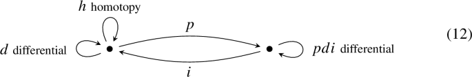
  Using the differential pdi, the maps p and i are a homotopy equivalence.

• A homotopy equivalence between two complexes (C, d) and $(C',d')$ are maps $R \in {{\,\mathrm{Hom}\,}}^0(C,C')$, $L \in {{\,\mathrm{Hom}\,}}^0(C',C)$, ${u}\in {{\,\mathrm{End}\,}}^{-1}(C)$, ${u}' \in {{\,\mathrm{End}\,}}^{-1}(C')$ where R, L are chain maps and $L R = \mathbbm {1}- d{u}- {u}d$ and $RL = \mathbbm {1}- d'{u}'-{u}'d'$. All four maps are part of the data. Note that R, L are quasi-isomorphisms. Compositions of homotopy equivalences are homotopy equivalences.

We often require that a homotopy satisfy $dhd = d$. Then the images of the projections in (11) are respectively ${{\,\mathrm{im}\,}}d$, a complement of ${{\,\mathrm{im}\,}}d$ in $\ker d$, and a complement of $\ker d$. Conversely, for every choice of two such graded complements there is a unique corresponding such homotopy.²¹ For a contraction, $dhd=d$ is equivalent to $di = 0$ or $pd = 0$ or $pdi = 0$. In this case the space on the right in (12) is canonically isomorphic, via i and p, to the homology of d.

Homological perturbation lemma. Given a contraction and a perturbation of the differential, the HPL produces a contraction for the perturbed differential. Explicitly, if the perturbed differential is called $d'$, and if we abbreviate $\delta = d'-d$, then

$$\begin{aligned} h' = h(\mathbbm {1} + \delta h)^{-1} \qquad i' = (\mathbbm {1} + h \delta )^{-1} i \qquad p' = p(\mathbbm {1} + \delta h)^{-1} \end{aligned}$$

(13)

is the new contraction if $\delta$ is suitably small so that the inverses are defined. The HPL keeps the spaces fixed and only perturbs the arrows in (12). Beware that $dhd=d$ does not imply $d'h'd'=d'$.²² See [23] for an exposition. One may think of $h-h' = h'(d'-d)h$ as analogous to Hilbert’s resolvent identity.

Differential graded Lie algebra and MC-elements. A graded Lie algebra or gLa is a $\mathbbm {Z}$-graded vector space ${{\mathfrak {g}}}$ with a bracket $[-,-] \in {{\,\mathrm{Hom}\,}}^0({{\mathfrak {g}}}\otimes {{\mathfrak {g}}},{{\mathfrak {g}}})$ that respects the grading, is graded antisymmetric, and satisfies the graded Jacobi identity. Explicitly for all homogeneous elements, the degree of [x, y] is the sum of the degrees of x and y and $[x,y] = -(-1)^{xy}[y,x]$ and

$$\begin{aligned}{}[x,[y,z]] + (-1)^{x(y+z)}[y,[z,x]] + (-1)^{z(x+y)}[z,[x,y]] = 0 \end{aligned}$$

(14)

A differential graded Lie algebra or dgLa ${{\mathfrak {g}}}$ is a gLa with $d \in {{\,\mathrm{End}\,}}^1({{\mathfrak {g}}})$ a differential, $d^2 = 0$, compatible with the bracket in the sense of the Leibniz rule $d[x,y] = [dx,y] + (-1)^x[x,dy]$. The Maurer–Cartan set is

$$\begin{aligned} {{\,\mathrm{MC}\,}}({{\mathfrak {g}}}) = \{u \in {{\mathfrak {g}}}^1 \mid du + \tfrac{1}{2}[u,u] = 0\} \end{aligned}$$

(15)

Formally, the Lie algebra ${{\mathfrak {g}}}^0$ acts on this set, and ${{\,\mathrm{MC}\,}}({{\mathfrak {g}}})/{\sim }$ is the moduli space of interest, a rigorous variant of which is the deformation functor [13].

Lie algebra of the Lorentz group and its representations. Given a 4-dimensional complex vector space with a nondegenerate quadratic form ${Q}$, the automorphism Lie algebra is ${\mathfrak {sl}}_{2}\oplus {\mathfrak {sl}}_{2}$ with ${\mathfrak {sl}}_{2}$ the complex Lie algebra of traceless $2 \times 2$ matrices. If the vector space is that of $2 \times 2$ complex matrices²³

$$\begin{aligned} k = \begin{pmatrix} a &{} b \\ c &{} d \end{pmatrix} \end{aligned}$$

and ${Q}= \det k = ad-bc$, then left- and right-multiplication by matrices with determinant one yield all automorphisms. Define right-multiplication with a transpose to get a left-action. At the Lie algebra level, ${\mathfrak {sl}}_{2}\oplus {\mathfrak {sl}}_{2}$. The finite-dimensional irreducible representations are

$$\begin{aligned} {(}p,q{)} = S^{2p}{(}\tfrac{1}{2},0{)} \otimes S^{2q}{(}0,\tfrac{1}{2}{)} \end{aligned}$$

where $p,q \ge 0$ are half-integers, ${(}\tfrac{1}{2},0{)} \simeq \mathbbm {C}^2$ and ${(}0,\tfrac{1}{2}{)} \simeq \mathbbm {C}^2$ are the fundamental representations of left and right ${\mathfrak {sl}}_{2}$ respectively, and S is the symmetric tensor product. So $\dim {(}p,q{)} = (2p+1)(2q+1)$. As ${\mathfrak {sl}}_{2}\oplus {\mathfrak {sl}}_{2}$ representations,

$$\begin{aligned} {(}p,q{)} \otimes {(}p',q'{)} \;\simeq \; \textstyle \bigoplus _{p'' = |p-p'|}^{p+p'} \bigoplus _{q''=|q-q'|}^{q+q'} {(}p'',q''{)} \end{aligned}$$

(16)

where $p''$ and $q''$ increase in steps of one. The Lie algebra ${\mathfrak {sl}}_{2}\oplus {\mathfrak {sl}}_{2}$ is the complexification of the real Lie algebra of the Lorentz group: On the real subspace of Hermitian $2 \times 2$ matrices, ${Q}$ is a real quadratic form of signature ${+}{-}{-}{-}$ whose automorphism Lie algebra is the real subalgebra of ${\mathfrak {sl}}_{2}\oplus {\mathfrak {sl}}_{2}$ of elements of the form $A \oplus {\overline{A}}$ where a bar means element-wise conjugation.

The Lorentz equivariant complexes ${\varGamma }_{\pm h}$. For every half-integer²⁴$h \ge \tfrac{1}{2}$ called helicity and for every momentum $k \in {(}\tfrac{1}{2},\tfrac{1}{2}{)} \simeq \mathbbm {C}^4$ define complexes

$$\begin{aligned} \begin{aligned} {\varGamma }_{h} :&\qquad 0 \rightarrow {(}h,0{)} \rightarrow {(}h-\tfrac{1}{2},\tfrac{1}{2}{)} \rightarrow {(}h-1,0{)} \rightarrow 0\\ {\varGamma }_{-h} :&\qquad 0 \rightarrow {(}0,h{)} \rightarrow {(}\tfrac{1}{2},h-\tfrac{1}{2}{)} \rightarrow {(}0,h-1{)} \rightarrow 0 \end{aligned} \end{aligned}$$

(17)

where, by definition, the three terms are in homological degrees 1, 2, 3 respectively and where the last term is dropped when $h = \frac{1}{2}$. The dependence on k is implicit in the differential. By definition, the differential is linear in $k \in {(}\tfrac{1}{2},\tfrac{1}{2}{)}$ and it is the unique ${\mathfrak {sl}}_{2}\oplus {\mathfrak {sl}}_{2}$ equivariant map

$$\begin{aligned} {(}\tfrac{1}{2},\tfrac{1}{2}{)} \otimes {(}h,0{)} \rightarrow {(}h-\tfrac{1}{2},\tfrac{1}{2}{)} \qquad {(}\tfrac{1}{2},\tfrac{1}{2}{)} \otimes {(}h-\tfrac{1}{2},\tfrac{1}{2}{)} \rightarrow {(}h-1,0{)} \end{aligned}$$

for ${\varGamma }_{h}$, analogous for ${\varGamma }_{-h}$. The uniqueness is by (16) and is up to an irrelevant multiplicative constant. This is a differential because its square is an equivariant map $S^2{(}\tfrac{1}{2},\tfrac{1}{2}{)} \otimes {(}h,0{)} \rightarrow {(}h-1,0{)}$ that vanishes by $S^2{(}\tfrac{1}{2},\tfrac{1}{2}{)} \simeq {(}0,0{)} \oplus {(}1,1{)}$ and (16). Explicitly, for ${\varGamma }_{\pm h}$ the first part of the differential is given by

$$\begin{aligned} S^{2h}\mathbbm {C}^2 \xrightarrow {\;\text {split}\;} S^{2h-1}\mathbbm {C}^2 \otimes \mathbbm {C}^2 \xrightarrow {\mathbbm {1}\otimes k^\mp \epsilon } S^{2h-1}\mathbbm {C}^2 \otimes \mathbbm {C}^2 \end{aligned}$$

(18a)

and the second is given by

$$\begin{aligned} S^{2h-1}\mathbbm {C}^2 \otimes \mathbbm {C}^2 \xrightarrow {\;\text {split}\;\otimes \mathbbm {1}} (S^{2h-2}\mathbbm {C}^2 \otimes \mathbbm {C}^2) \otimes \mathbbm {C}^2 \simeq S^{2h-2}\mathbbm {C}^2 \otimes (\mathbbm {C}^2 \otimes \mathbbm {C}^2)\nonumber \\ \xrightarrow {\mathbbm {1}\otimes (\epsilon k^{\pm } \epsilon )} S^{2h-2}\mathbbm {C}^2 \end{aligned}$$

(18b)

where $k = ({\begin{matrix} a &{} b \\ c &{} d \end{matrix}})$ and $\epsilon = ({\begin{matrix} 0 &{} 1 \\ -1 &{} 0 \end{matrix}})$ and $k^+ = k$ and $k^- = k^T$, splitting means $z^{\otimes p} \mapsto z^{\otimes p-1} \otimes z$ for all $z \in \mathbbm {C}^2$, and $\epsilon k^{\pm } \epsilon : \mathbbm {C}^2 \otimes \mathbbm {C}^2 \rightarrow \mathbbm {C}$, $x \otimes y \mapsto x^T\epsilon k^\pm \epsilon y$.²⁵ More explicitly still, there are bases for which the differential for ${\varGamma }_2$ is

$$\begin{aligned} \left( {\begin{matrix} a &{}\quad c &{}\quad 0 &{}\quad 0 &{}\quad 0 \\ b &{}\quad d &{}\quad 0 &{}\quad 0 &{}\quad 0 \\ 0 &{}\quad a &{}\quad c &{}\quad 0 &{}\quad 0 \\ 0 &{}\quad b &{}\quad d &{}\quad 0 &{}\quad 0 \\ 0 &{}\quad 0 &{}\quad a &{}\quad c &{}\quad 0 \\ 0 &{}\quad 0 &{}\quad b &{}\quad d &{}\quad 0 \\ 0 &{}\quad 0 &{}\quad 0 &{}\quad a &{}\quad c \\ 0 &{}\quad 0 &{}\quad 0 &{}\quad b &{}\quad d\end{matrix}}\right) \qquad \text {and} \qquad \left( {\begin{matrix} b &{}\quad -a &{}\quad d &{}\quad -c &{}\quad 0 &{}\quad 0 &{}\quad 0 &{}\quad 0\\ 0 &{}\quad 0 &{}\quad b &{}\quad -a &{}\quad d &{}\quad -c &{}\quad 0 &{}\quad 0\\ 0 &{}\quad 0 &{}\quad 0 &{}\quad 0 &{}\quad b &{}\quad -a &{}\quad d &{}\quad -c \end{matrix}}\right) \end{aligned}$$

(19)

Switch b, c for ${\varGamma }_{-2}$. Similar for ${\varGamma }_{\pm h}$. The homologies are in Lemmas 12 and 22 . Briefly, for $k\ne 0$ there is homology only when ${Q}=0$, that is, when $k=vw^T$ with $v,w \in \mathbbm {C}^2$. The homology is $0 \rightarrow \mathbbm {C}\rightarrow \mathbbm {C}\rightarrow 0 \rightarrow 0$ there. A representative for $H^1({\varGamma }_h)$ is $v^{\otimes 2h}$, one for $H^1({\varGamma }_{-h})$ is $w^{\otimes 2h}$.

3 Part I: Amplitudes as $L_\infty$ Minimal Model Brackets

4 The $L_\infty$ Minimal Model Reviewed

Homotopy transfer refers generally to the transfer of certain algebraic structures through quasi-isomorphisms, see e.g. [8]. In the special case of a dgLa ${{\mathfrak {g}}}$ and a contraction to the homology ${{{\mathfrak {h}}}}$, one obtains an $L_\infty$ algebra structure on ${{{\mathfrak {h}}}}$ called the $L_\infty$ minimal model, unique up to $L_\infty$ isomorphisms. We recall explicit formulas for the $L_\infty$ minimal model brackets as a sum of trivalent trees. We refer to the literature for proofs that they define the $L_\infty$ minimal model, including formulas for suitable $L_\infty$ quasi-isomorphisms [8, 13,14,15,16].

Let $T_n$ be the set of tree graphs with $n+1$ labeled leaves, $n-2$ unlabeled internal lines, $n-1$ internal nodes of degree 3 (known as trivalent or cubic). The leaves $1,\ldots ,n$ are called inputs, and $n+1$ the output. Let $P_n$ be the set of such trees with a planar embedding. The canonical map $P_n \rightarrow T_n$ that forgets the embedding is surjective.²⁶

Definition 2

(Trees). For a dgLa ${{\mathfrak {g}}}$ and a homotopy h (see Sect. 2) that satisfies $dhd = d$, let $p: {{\mathfrak {g}}}\rightarrow {{{\mathfrak {h}}}}$ and $i: {{{\mathfrak {h}}}}\rightarrow {{\mathfrak {g}}}$ be the unique associated contraction. For every $P \in P_n$ define $m_{P,h} \in {{\,\mathrm{Hom}\,}}^{2-n}({{{\mathfrak {h}}}}^{\otimes n},{{{\mathfrak {h}}}})$ as follows:

• Decorate each input leaf by i, the output leaf by p.

• Decorate each internal line by h.

• Decorate each node by $\llbracket -,-\rrbracket$. Here $\llbracket x,y\rrbracket = (-1)^x [x,y]$ for all $x,y \in {{\mathfrak {g}}}$.

• Given $x_1 \otimes \cdots \otimes x_n \in {{{\mathfrak {h}}}}^{\otimes n}$ one inserts each $x_j$ at the input labeled j.

• Multiply by the sign needed to permute $x_1,\ldots ,x_n$ into place, where an even (odd) $x_j$ is considered odd (even) for the purpose of this permutation.²⁷

• Multiply by the sign $(-1)^{x_{n-1} + x_{n-3} + x_{n-5} + \cdots }$.²⁸

Then $m_{P,h}$ is independent of the planar embedding.²⁹ So for every $T \in T_n$ we can set $m_{T,h} = m_{P,h}$ where $P \in P_n$ is any planar embedding of T.

Example 2

The set $P_n$ is in bijection with full parenthesizations of any permutation of the elements $1,\ldots ,n$. With this understanding,

$$\begin{aligned} m_{(12),h}(x_1,x_2)&= p[ix_1,ix_2]\\ m_{((((12)3)4)5),h}(x_1,\ldots ,x_5)&= p[h[h[h[ix_1,ix_2],ix_3],ix_4],ix_5]\\ m_{(((12)3)(45)),h}(x_1,\ldots ,x_5)&= (-1)^{1+x_1+x_2+x_3} p[h[h[ix_1,ix_2],ix_3],h[ix_4,ix_5]] \end{aligned}$$

Note that if all inputs have odd degree, one always gets a plus sign.

Definition 3

(Minimal model brackets associated to a homotopy). For a dgLa ${{\mathfrak {g}}}$ and a homotopy h as above, the n-slot minimal model bracket

$$\begin{aligned} \{-,\ldots ,-\}_h \;=\; \textstyle \sum _{T \in T_n} m_{T,h} \end{aligned}$$

is in ${{\,\mathrm{Hom}\,}}^{2-n}({{{\mathfrak {h}}}}^{\otimes n},{{{\mathfrak {h}}}})$. It satisfies $\{\ldots ,y,x,\ldots \}_h = -(-1)^{xy} \{\ldots ,x,y,\ldots \}_h$.

5 The $L_\infty$ Minimal Model is Gauge Independent

The minimal model of a dgLa is unique up to $L_\infty$ isomorphism [13]. Here we show a more special but stronger statement: For a dgLa ${{\mathfrak {g}}}$ with a momentum grading, the minimal model brackets associated to different momentum conserving homotopies are equal, when all internal lines are off-shell, not merely isomorphic. Individual trees depend on the homotopy, but the sum of all trees does not. We identify a minimal set of assumptions that imply such a result, for maximal flexibility later on. The result is for all homological degrees.

Definition 4

(Momentum grading). Suppose K is an Abelian group that we call momentum space. By a dgLa ${{\mathfrak {g}}}= \bigoplus _{i\in \mathbbm {Z}} {{\mathfrak {g}}}^i$ with momentum grading we mean one that carries a compatible K-grading, with algebraic direct sum

$$\begin{aligned} {{\mathfrak {g}}}= \textstyle \bigoplus _{k \in K} {{\mathfrak {g}}}_k \end{aligned}$$

Compatibility means that the K-grading respects the $\mathbbm {Z}$-grading and that

$$\begin{aligned} d {{\mathfrak {g}}}_k \subseteq {{\mathfrak {g}}}_k \qquad \qquad [{{\mathfrak {g}}}_{k_1},{{\mathfrak {g}}}_{k_2}] \subseteq {{\mathfrak {g}}}_{k_1+k_2} \end{aligned}$$

Then the homology of ${{\mathfrak {g}}}$ also decomposes, ${{{\mathfrak {h}}}}= \bigoplus _{k \in K} {{{\mathfrak {h}}}}_k$ where ${{{\mathfrak {h}}}}_k$ is the homology of ${{\mathfrak {g}}}_k$. A momentum k is called on-shell if ${{{\mathfrak {h}}}}_k \ne 0$, off-shell if ${{{\mathfrak {h}}}}_k = 0$.

In this section, ${{\mathfrak {g}}}$ is a dgLa with momentum grading. We always assume that homotopies are momentum conserving, $h{{\mathfrak {g}}}_k\subseteq {{\mathfrak {g}}}_k$ for all $k\in K$. Then, the minimal model bracket in Definition 3 is a map ${{{\mathfrak {h}}}}_{k_1} \otimes \cdots \otimes {{{\mathfrak {h}}}}_{k_n} \rightarrow {{{\mathfrak {h}}}}_{k_1 + \ldots + k_n}$. In the case $n=5$ it uses trees like in Fig. 3, where $h_k = h|_{{{\mathfrak {g}}}_k}$.

Fig. 3

An $n=5$ tree with momentum conserving homotopies

Remark 1

(Discontinuous nature of h). The space K has no topology and no continuity in k is assumed. In our application, $K=\mathbbm {C}^4$ and the homotopy h is discontinuous, separately defined off-shell and on-shell.

Theorem 5

(Gauge independence I). The bracket $\{-,\ldots ,-\}_h$ is independent of the momentum-conserving homotopy h when evaluated on

$$\begin{aligned} {{{\mathfrak {h}}}}_{k_1} \otimes \cdots \otimes {{{\mathfrak {h}}}}_{k_n} \rightarrow {{{\mathfrak {h}}}}_{k_1 + \ldots + k_n} \end{aligned}$$

with all internal lines off-shell, meaning for all $(k_1,\ldots ,k_n) \in K^n$ such that ${{{\mathfrak {h}}}}_{k_J}=0$ for all subsets $J \subseteq \{1,\ldots ,n\}$ with $1< |J| < n$ and $k_J = \sum _{i \in J} k_i$.

The proof of Theorem 5 is at the end of this section. We need a tool to connect different homotopies, that is, different gauge choices. The following lemma, which is for any complex of vector spaces, connects any two homotopies h and $h'$ by three transformations. We will use it to connect the homotopies by three curves polynomial in a parameter s. Pictorially,

Lemma 1

(ABC lemma). Consider a complex with differential d. In this lemma we only consider homotopies h that satisfy $dhd=d$, and we denote $\pi = \mathbbm {1}- dh - hd$. If h is a homotopy then another homotopy $h'$ is given by

for all ${a},{c}\in {{\,\mathrm{End}\,}}^0({{\mathfrak {g}}})$ or ${b}\in {{\,\mathrm{End}\,}}^{-2}({{\mathfrak {g}}})$ respectively, subject to the constraints. And any two homotopies h and $h'$ are related by a composition of $\mathcal {{A}}$, $\mathcal {{B}}$, $\mathcal {{C}}$. Namely, if one sets $h_{A}= \mathcal {{A}}h$ and $h_{B}= \mathcal {{B}}h_{A}$ and $h_{C}= \mathcal {{C}}h_{B}$ with

$$\begin{aligned} {a}= -dh'\pi \qquad {b}= -h_{A}dh'h_{A}\qquad {c}= -\pi _{B}h'd \end{aligned}$$

(20)

then $h_{C}= h'$.

Proof

First the transformations in the table. For $\mathcal {{C}}$ we have $(h')^2 = 0$ using $h^2 = 0$, $h\pi = 0$, we have $h'dh' = h'$ using $hdh = h$, $d\pi = 0$, we have $dh'd = d$ using $dhd = d$, $d\pi = 0$, and $\pi ' = \mathbbm {1}- h'd-dh'$. Similar for $\mathcal {{A}}$, $\mathcal {{B}}$. Before proving the second part of the theorem, we derive another characterization of $\mathcal {{A}}$, $\mathcal {{B}}$, $\mathcal {{C}}$.

Note that $\mathcal {{A}}$ implies $hd = h'd$, $\mathcal {{B}}$ implies $\pi = \pi '$, $\mathcal {{C}}$ implies $dh = dh'$. Conversely, for all h and $h'$, if $hd=h'd$ then they are related by $\mathcal {{A}}$ using ${a}= -d h'\pi$, if $\pi = \pi '$ then by $\mathcal {{B}}$ using ${b}= -hdh'h$, if $dh=dh'$ then by $\mathcal {{C}}$ using ${c}= -\pi h'd$. Say in the case $\mathcal {{A}}$, the given ${a}$ has degree zero, satisfies the constraints in the table, and $h(\mathbbm {1}-{a}\pi ) = h(\mathbbm {1}+ dh'\pi ) = h + hdh'\pi = h + h'dh'\pi = h + h'\pi = h + h'(\mathbbm {1}-dh-hd) = h'$ as required using $h'hd = h'h'd = 0$ and $h'dh = hdh = h$. Similar for $\mathcal {{B}}$, $\mathcal {{C}}$. The constraints make ${a},{b},{c}$ unique.

Though one can proceed at the level of equations, we switch to a geometric argument. Recall the bijection between homotopies h with $dhd=d$ and pairs (X, Y) of graded subspaces where X is a complement of ${{\,\mathrm{im}\,}}d$ in $\ker d$, Y a complement of $\ker d$. The bijection is given by $X = {{\,\mathrm{im}\,}}\pi$, $Y = {{\,\mathrm{im}\,}}hd$. The last paragraph shows that $\mathcal {{A}}$ connects any two homotopies with the same Y, $\mathcal {{B}}$ those with the same X and $Y \oplus {{\,\mathrm{im}\,}}d$, $\mathcal {{C}}$ those with the same X and $Y\oplus X$.

Now, given any two homotopies h, $h'$ corresponding to (X, Y), $(X',Y')$ respectively, define homotopies $h_{A}$, $h_{B}$, $h_{C}$ by $X_{A}= X_{B}= X_{C}= X'$, $Y_{A}= Y$, $Y_{C}= Y'$, and $Y_{B}$ is given by $Y\oplus {{\,\mathrm{im}\,}}d = Y_{B}\oplus {{\,\mathrm{im}\,}}d$ and $Y_{B}\oplus X'=Y'\oplus X'$. There exists a unique such $Y_{B}$ since Y and $Y'$ are complements of $\ker d = {{\,\mathrm{im}\,}}d\oplus X'$. By the last paragraph we have $h_{A}= \mathcal {{A}}h$, $h_{B}= \mathcal {{B}}h_{A}$, $h_{C}= \mathcal {{C}}h_{B}$ for some $\mathcal {{A}}$, $\mathcal {{B}}$, $\mathcal {{C}}$. One can see that they are given by (20). By construction, $h_{C}=h'$. $\quad \square$

Theorem 6

(Gauge independence II). Let $M_h \in {{\,\mathrm{Hom}\,}}^{2-n}({{\mathfrak {g}}}^{\otimes n},{{\mathfrak {g}}})$ be defined like the minimal model brackets but with input and output leaves decorated by $\pi = \mathbbm {1}- dh - hd$, replacing i and p. Let $d_{\text {tot}}$ be the differential on ${{\mathfrak {g}}}^{\otimes n}$, so

$$\begin{aligned} d_{\text {tot}}= \textstyle \sum _{i=1}^n (\pm \mathbbm {1})^{\otimes (i-1)} \otimes d \otimes \mathbbm {1}^{\otimes (n-i)} \end{aligned}$$

where $\pm \mathbbm {1}$ is the sign map. Then for all homotopies h and $h'$ there exists a linear map $E: {{\mathfrak {g}}}^{\otimes n} \rightarrow {{\mathfrak {g}}}$ (that can be given as a sum of trees built using only h and $h'$ and d and the bracket) such that

$$\begin{aligned} M_{h'} - M_h \qquad \text {equals} \qquad dE + Ed_{\text {tot}}\end{aligned}$$

when evaluated on ${{\mathfrak {g}}}_{k_1} \otimes \cdots \otimes {{\mathfrak {g}}}_{k_n} \rightarrow {{\mathfrak {g}}}_{k_1 + \ldots + k_n}$ with all internal lines off-shell, where off-shell means homology-free just like in Theorem 5.

Proof

It suffices to prove the theorem in the special cases $\mathcal {{A}}$, $\mathcal {{B}}$, $\mathcal {{C}}$ of Lemma 1. Since $h{{\mathfrak {g}}}_k \subseteq {{\mathfrak {g}}}_k$, (20) implies ${a}{{\mathfrak {g}}}_k, {b}{{\mathfrak {g}}}_k, {c}{{\mathfrak {g}}}_k\subseteq {{\mathfrak {g}}}_k$. The brackets are polynomial in h and $\pi$, so if we consider polynomial curves ${a}(s)$, ${b}(s)$, ${c}(s)$ then the brackets are polynomial in s. It suffices to show that we get the desired result when differentiating with respect to s, namely that ${\dot{M}} = d{\dot{E}} + {\dot{E}}d_{\text {tot}}$ for some ${\dot{E}}$ where a dot denotes a derivative at $s=0$:³⁰

• $\mathcal {{A}}$. Here ${\dot{h}} = -h{\dot{{a}}}\pi$ and ${\dot{\pi }} = dh{\dot{{a}}} \pi$. Since all internal lines are off-shell hence annihilated by $\pi$, we effectively have ${\dot{h}} = 0$. So only inputs and outputs are affected. One can take ${\dot{E}} = h{\dot{{a}}} M$ in this case.

• $\mathcal {{B}}$. Here ${\dot{h}} = d{\dot{{b}}}dh-hd{\dot{{b}}}d = d{\dot{{b}}} - {\dot{{b}}}d$ and ${\dot{\pi }} = 0$. In particular, only internal lines are affected. Here ${\dot{E}} = 0$.

• $\mathcal {{C}}$. Here ${\dot{h}} = -\pi {\dot{{c}}} h$ and ${\dot{\pi }} = \pi {\dot{{c}}} hd$. As in $\mathcal {{A}}$, we effectively have ${\dot{h}} = 0$. Here ${\dot{E}} = M {\dot{{C}}}$ where ${\dot{{C}}}$ is a graded symmetrization of ${\dot{{c}}} h \otimes \mathbbm {1}^{\otimes n-1}$.

With this setup, it suffices to show for every nonempty $J \subseteq \{1,\ldots ,n\}$ that the following infinitesimal variations, affecting internal lines with momentum $k_J = \sum _{i \in J} k_i$, yield zero after summation over all trees:

• Variations of type $d{\dot{{b}}}$ at an internal line if $1< |J| < n$ respectively $dh{\dot{{a}}}\pi$ at the input if $|J| = 1$. Note the d on the left.

• Variations of type $-{\dot{{b}}}d$ at an internal line if $1< |J| < n$, respectively $\pi {\dot{{c}}} hd$ at the output if $|J| = n$. Note the d on the right.

All cases reduce to Lemma 2. Given the results for ${\dot{E}}$, one can see that E has the claimed form. For $\mathcal {{A}}$ take $E=haM$, for $\mathcal {{B}}$ take $E=0$, similar for $\mathcal {{C}}$. $\quad \square$

Lemma 2

(A cancellation). The map ${{\mathfrak {g}}}_{k_1} \otimes \cdots \otimes {{\mathfrak {g}}}_{k_n} \rightarrow {{\mathfrak {g}}}_{k_1 + \cdots + k_n}$ defined just like M but with the output leaf decorated by Nd (rather than $\pi$) is identically zero when all internal lines are off-shell. Likewise if one input leaf is decorated by dN. Here N is any momentum conserving operator of degree $-1$ to guarantee that Nd respectively dN have degree zero.³¹

Proof

When d is the output, and all inputs are odd, then this is the lemma in dgLa-based deformation theory that says that obstructions are cocycles [24]. In general, when the output is decorated by Nd, the proof is by repeatedly moving occurrences of d down the trees using this algorithm:

$$\begin{aligned} \left. \begin{aligned}&\text {If }d \text { hits a bracket as in }d[-,-],\text { use the Leibniz rule.}\\&\text {If }d \text { hits an }h, \text {replace }dh = - hd - \pi + \mathbbm {1}.\\ {}&\text {Terms from}\, \pi \text { vanish since }\pi \text { annihilates off-shell momenta.}\\&\text {Terms from }\mathbbm {1}\text { are put in a basket, to be dealt with later.}\\&\text {If }d \text { hits an input }\pi , \text { use }d\pi = 0. \end{aligned}\;\;\;\right\} \end{aligned}$$

(21)

We must show that the terms in the basket add to zero. These terms are one-to-one with $T_n'$, the set of trees like $T_n$ but with a distinguished internal line. The distinguished line is the one decorated by $\mathbbm {1}$, corresponding to a direct nesting of two brackets as in $[[-,-],-]$. Define an equivalence relation on $T_n'$ that identifies trees that differ only by a permutation of the four lines adjacent to the distinguished line. Each equivalence class has three elements as in

where $t_R,t_A,t_B,t_C$ are subtrees and we agree that a planar embedding is chosen for each inducing an embedding for the three terms, and the output leaf is in $t_R$. These three terms are $\sigma \llbracket \llbracket A,B \rrbracket ,C\rrbracket$ and $\sigma ' \llbracket \llbracket B,C\rrbracket ,A\rrbracket$ and $\sigma ''\llbracket \llbracket C,A \rrbracket ,B \rrbracket$, inserted into the operator given by $t_R$. Their relative signs are

$$\begin{aligned} \sigma : \sigma ' : \sigma '' = 1 :(-1)^{(A+1)(B+C)} : (-1)^{(C+1)(A+B)} \end{aligned}$$

and so they add to zero by the definition of $\llbracket -,-\rrbracket$ and the Jacobi identity. The relative signs are due to the permutation sign in Definition 2, since $A+1$, $B+1$, $C+1$ are equal to the number of even elements entering $t_A$, $t_B$, $t_C$ respectively, mod 2. No relative sign was produced by algorithm (21), in particular the last application of the Leibniz rule is without sign since $\mathbbm {1}$ is left-adjacent to $t_R$.

Analogous if dN decorates an input leaf, in this case one repeatedly moves occurrences of d away from that input, a modification of (21). Suppose that input is in $t_A$. We get zero again since the relative signs are

$$\begin{aligned} \sigma : \sigma ' : \sigma '' = \underline{(-1)} : \underline{(-1)^{B+C+1}} (-1)^{A(B+C)} : \underline{(-1)^C} (-1)^{(C+1)(A+B+1)} \end{aligned}$$

because the number of even elements entering $t_A$ is now A mod 2 due to the presence of the operator N, and the underlined relative signs are introduced by the final application of the Leibniz rule. $\quad \square$

Proof of Theorem 5

Recall $M_h : {{\mathfrak {g}}}^{\otimes n} \rightarrow {{\mathfrak {g}}}$ in Theorem 6. It is a chain map, $dM_h = M_hd_{\text {tot}}$, because $d\pi = \pi d = 0$. It induces the minimal model bracket $\{-,\ldots ,-\}_h:{{{\mathfrak {h}}}}^{\otimes n} \rightarrow {{{\mathfrak {h}}}}$ on homology, since $\pi i = (i p) i = i (p i) = i$, analogously $p \pi = p$. By Theorem 6, $M_h$ and $M_{h'}$ are homotopy equivalent when internal lines are off-shell. Therefore they induce the same map on homology. $\quad \square$

6 YM and GR in Terms of a Differential Graded Lie Algebra

Here we recall constructions in [9,10,11] for YM and [12] for GR. We introduce two differential graded Lie algebras ${{\mathfrak {g}}}^\infty$ whose Maurer–Cartan equation are the classical field equations of YM respectively GR about Minkowski spacetime $\mathbbm {R}^4$. In particular, for GR the solutions are the Ricci-flat metrics.

We begin with YM. Here it is natural to first define a differential graded commutative associative algebra (dgca) ${{\mathfrak {a}}}^\infty$. Preliminaries:

• $C^\infty = C^\infty (\mathbbm {R}^4)$ are the smooth complex valued functions of $x \in \mathbbm {R}^4$.

• $\varOmega$ is the dgca of complex de Rham differential forms on $\mathbbm {R}^4$ with the de Rham differential. So $\varOmega = C^\infty \otimes \wedge \mathbbm {C}^4$ where $\wedge \mathbbm {C}^4$ is the unital gca freely generated in degree one by the symbols $dx^0,dx^1,dx^2,dx^3$.

• Decompose $\varOmega ^2 = \varOmega ^2_+ \oplus \varOmega ^2_-$ where $\varOmega ^2_{\pm }$ is the $C^\infty$-submodule generated by all $dx^0 dx^a \pm i\,dx^b dx^c$ with a, b, c a cyclic permutation of 1, 2, 3.

• Set $\varOmega ^{\le 2}_{\pm } = \varOmega ^0 \oplus \varOmega ^1 \oplus \varOmega ^2_{\pm }$ and $\varOmega _{\pm }^{\ge 2} = \varOmega ^2_{\pm } \oplus \varOmega ^3 \oplus \varOmega ^4$.

Remark 2

Recall that there are natural tensor products $\text {dgca}\otimes \text {dgca}= \text {dgca}$ and $\text {dgca}\otimes \text {dgLa}= \text {dgLa}$ that, at the level of complexes, correspond to the usual tensor product of complexes. If A, B are dgca then on $A \otimes B$ use the gca product $(a\otimes b)(a' \otimes b') = (-1)^{ba'} (aa') \otimes (bb')$. If A is a dgca and P is a dgLa then on $A \otimes P$ use the gLa bracket $[a \otimes p,a'\otimes p'] = (-1)^{pa'} (aa') \otimes [p,p']$.

Proposition 1

(YM dgca). Let $\mathbbm {C}\oplus \mathbbm {C}\epsilon$ be the dgca with $\epsilon$ a symbol of degree $-1$, product given by $\epsilon ^2 = 0$, and differential $z \oplus w\epsilon \mapsto w \oplus 0\epsilon$. Then the tensor product of dgca $(\mathbbm {C}\oplus \mathbbm {C}\epsilon ) \otimes \varOmega \simeq \varOmega \oplus \epsilon \varOmega$ (see Remark 2) has a dgca subquotient

$$\begin{aligned} {{\mathfrak {a}}}^\infty = \frac{\varOmega \oplus \epsilon \varOmega _+^{\ge 2}}{ \varOmega _-^{\ge 2} \oplus \epsilon 0} \end{aligned}$$

(22)

That is, the numerator is a sub-dgca of $\varOmega \oplus \epsilon \varOmega$, and the denominator is a dgca ideal in the numerator. It follows that ${{\mathfrak {a}}}^\infty$ is itself a dgca.

Proof

The dgca axioms hold for $\mathbbm {C}\oplus \mathbbm {C}\epsilon$. And (22) is a dgca subquotient:

• The numerator is a subcomplex of $\varOmega \oplus \epsilon \varOmega$, this is clear.

• The numerator is a subalgebra of $\varOmega \oplus \epsilon \varOmega$, since $\varOmega \varOmega _+^2 \subseteq {\varOmega _+^{\ge 2}}$.

• The denominator is a subcomplex of the numerator, this is clear.

• The denominator is an algebra ideal in the numerator, since $\varOmega _+^2 \varOmega _-^2 = 0$.$\quad \square$

Remark 3

As a $C^\infty$-module, ${{\mathfrak {a}}}^\infty \simeq \varOmega ^{\le 2}_+ \oplus \epsilon \varOmega _+^{\ge 2}$, which more explicitly is, with $d_\varOmega$ denoting the de Rham differential and $\pi _+ : \varOmega ^2 \rightarrow \varOmega ^2_+$ the projection:

Remark 4

Using the standard basis for $\varOmega$ and the basis for $\varOmega _+^2$ given before, we have ${{\mathfrak {a}}}^\infty = C^\infty \otimes {{V}}$ with ${{V}}\simeq \mathbbm {C}\oplus \mathbbm {C}^7 \oplus \mathbbm {C}^7 \oplus \mathbbm {C}$ with summands in homological degrees 0, 1, 2, 3 respectively. The differential is a constant coefficient first order differential operator, the product is bilinear over $C^\infty$.

Proposition 2

(YM dgLa). The tensor product of the dgca ${{\mathfrak {a}}}^\infty$ with any finite-dimensional complex Lie algebra ${{\mathfrak {u}}}$ (see Remark 2, with the understanding that ${{\mathfrak {u}}}$ is here ungraded and carries the zero differential) yields a dgLa

$$\begin{aligned} {{\mathfrak {g}}}^\infty = {{\mathfrak {a}}}^\infty \otimes {{\mathfrak {u}}}\end{aligned}$$

The associated MC-equation yields ordinary YM with ‘internal’ Lie algebra ${{\mathfrak {u}}}$.

Proof

Let $u \in ({{\mathfrak {g}}}^\infty )^1$, so $u = A \oplus \epsilon F$ with $A \in \varOmega ^1 \otimes {{\mathfrak {u}}}$ and $F \in \varOmega ^2_+ \otimes {{\mathfrak {u}}}$. The MC-equations $du + \tfrac{1}{2}[u,u]=0$ are $d_\varOmega A + F + \tfrac{1}{2} [A,A] = 0$ in $\varOmega ^2/\varOmega ^2_- \otimes {{\mathfrak {u}}}$ and $d_\varOmega F + [A,F] = 0$ in $\varOmega ^3 \otimes {{\mathfrak {u}}}$ with $d_\varOmega$ the de Rham differential and the bracket is the product of forms and the bracket in ${{\mathfrak {u}}}$. These are the YM equations.³² See also Costello [11, Section 6.2]. $\quad \square$

Remark 5

Similar to Remark 4, ${{\mathfrak {g}}}^\infty = C^\infty \otimes {{V}}$ with ${{V}}\simeq (\mathbbm {C}\oplus \mathbbm {C}^7 \oplus \mathbbm {C}^7 \oplus \mathbbm {C}) \otimes {{\mathfrak {u}}}$.

We turn to GR. We define a gLa (and then via ‘twisting’ with the Minkowski element a dgLa) ${{\mathfrak {g}}}$ whose Maurer–Cartan equation is an orthonormal frame formulation of the vacuum Einstein equations, essentially identical to the Newman–Penrose formalism [25], and equivalent to the traditional formulation as the Ricci-flatness of a metric. Informally^33,34

$$\begin{aligned} \frac{\text {Ricci-flat metrics}}{\text {diffeomorphisms}} \;\;\simeq \;\; \frac{\text {Maurer--Cartan elements}}{\sim } \end{aligned}$$

(24)

This gLa is defined in [12], where a background-independent account is given. The account given here uses Minkowski spacetime as an auxiliary background structure and thereby obscures background independence. Furthermore, we directly define the version over the complex numbers $\mathbbm {C}$, but there is an obvious real structure at every step of the construction. As a preliminary, in the next lemma we recall a purely algebraic construction. As before, $\otimes = \otimes _{\mathbbm {C}}$.

Lemma 3

(Base change). Given a graded commutative algebra A, a Lie algebra P, and a Lie algebra map $P \rightarrow \mathrm {Der}^0(A)$, so a representation of P as $\mathbbm {C}$-linear derivations of degree zero, then $A \otimes P$ becomes a gLa by defining

(25)

for all $a,a' \in A$ and $p,p' \in P$. The grading is induced from the grading on A.

Proof

By direct verification, the bracket is well-defined, bilinear, graded antisymmetric, and satisfies the graded Jacobi identity (14). $\quad \square$

In a first step, we apply Lemma 3 with $\varOmega = C^\infty \otimes \wedge \mathbbm {C}^4$ in the role of A, and the direct sum of Lie algebras ${{\mathfrak {v}}}= \mathbbm {C}^4 \oplus {{\mathfrak {so}}_{1,3}}$ in the role of P.³⁵ The required Lie algebra map ${{\mathfrak {v}}}\rightarrow \mathrm {Der}^0(\varOmega )$ is defined as follows:

• The Abelian Lie algebra $\mathbbm {C}^4$ acts by differentiation on $C^\infty$ via the identification $\mathbbm {C}^4 \simeq \mathbbm {C}\partial _0 \oplus \mathbbm {C}\partial _1 \oplus \mathbbm {C}\partial _2 \oplus \mathbbm {C}\partial _3$ with $\partial _\mu = \frac{\partial }{\partial x^\mu }$ the partial derivatives on $\mathbbm {R}^4$; and it acts trivially on $\wedge \mathbbm {C}^4$.

• The Lie algebra³⁶${{\mathfrak {so}}_{1,3}}$ acts trivially on $C^\infty$; and it acts as the fundamental representation on $dx^0,dx^1,dx^2,dx^3$ which extends uniquely to an action as derivations of degree zero on $\wedge \mathbbm {C}^4$.

Lemma 4

(Auxiliary dgLa for GR and the Minkowski element).

• The tensor product of vector spaces $\varOmega \otimes {{\mathfrak {v}}}$ becomes a graded Lie algebra, with grading from $\varOmega$, by defining for all $\omega ,\omega ' \in \varOmega$ and $v,v' \in {{\mathfrak {v}}}$:

  

  (26)

• The ‘Minkowski’ element $m \in \varOmega ^1 \otimes {{\mathfrak {v}}}$ defined by

  $$\begin{aligned} m \;=\; dx^0 \otimes \partial _0 + dx^1 \otimes \partial _1 + dx^2 \otimes \partial _2 + dx^3 \otimes \partial _3 \end{aligned}$$

  (27)

  satisfies $[m,m] = 0$. The map $d = [m,-] \in {{\,\mathrm{End}\,}}^1(\varOmega \otimes {{\mathfrak {v}}})$ is a differential, and satisfies the Leibniz rule for the bracket, thus turns $\varOmega \otimes {{\mathfrak {v}}}$ into a dgLa.

Proof

The first part is a direct application of the base change in Lemma 3. To check $[m,m]=0$, note that (26) implies $[dx^a \otimes \partial _\mu , dx^b \otimes \partial _\nu ] =0$ for all $a,b,\mu ,\nu$ since, by the definition of ${{\mathfrak {v}}}\rightarrow \mathrm {Der}^0(\varOmega )$ above, $\partial _\mu$ acts trivially on $dx^b$ and $\partial _\nu$ acts trivially on $dx^a$, and furthermore $[\partial _\mu ,\partial _\nu ] = 0$. Given $[m,m]=0$, the statements about $d = [m,-]$ are standard and known as ’twisting’: To prove $d^2=0$, note that by (14) we have, for all homogeneous $y \in \varOmega \otimes {{\mathfrak {v}}}$:

$$\begin{aligned} {[}y,[m,m]] + \underbrace{ [m,[m,y]] - (-1)^y[m,[y,m]] }_{ =\, 2[m,[m,y]]} = 0 \end{aligned}$$

The first term vanishes, hence $[m,[m,y]]=0$ for all y, hence $d^2=0$. The Leibniz rule for d also follows from the graded Jacobi identity (14). $\quad \square$

The complex underlying the dgLa $\varOmega \otimes {{\mathfrak {v}}}$ is

$$\begin{aligned} 0 \rightarrow \varOmega ^0 \otimes {{\mathfrak {v}}}\rightarrow \varOmega ^1 \otimes {{\mathfrak {v}}}\rightarrow \varOmega ^2 \otimes {{\mathfrak {v}}}\rightarrow \varOmega ^3 \otimes {{\mathfrak {v}}}\rightarrow \varOmega ^4 \otimes {{\mathfrak {v}}}\rightarrow 0 \end{aligned}$$

This dgLa is not yet suitable for GR, but we want to become familiar with it before we continue. Clearly $\varOmega \otimes {{\mathfrak {v}}}$ is a module over $\varOmega$ by left-multiplication, but the differential is not linear over $\varOmega$, instead one has:

Lemma 5

($\varOmega \otimes {{\mathfrak {v}}}$ is an $\varOmega$-dg-module). For all $\omega \in \varOmega$ and $y \in \varOmega \otimes {{\mathfrak {v}}}$:

$$\begin{aligned} d(\omega y) \;=\; d_\varOmega (\omega ) y+ (-1)^\omega \omega dy \end{aligned}$$

(28)

Proof

This is a direct consequence of (26) and (27). $\quad \square$

By (28), we know how the differential d acts on any element of $\varOmega \otimes {{\mathfrak {v}}}$ if we know how it acts on the generators ${{\mathfrak {v}}}= \mathbbm {C}^4 \oplus {{\mathfrak {so}}_{1,3}}$. Beware that the differential d annihilates the summand $\mathbbm {C}^4$, but it does not annihilate ${{\mathfrak {so}}_{1,3}}$:

Example 3

Let $\sigma _{12} \in {{\mathfrak {so}}_{1,3}}$ be the infinitesimal rotation in the 12-plane:

$$\begin{aligned} \sigma _{12}(dx^0) = 0 \qquad \sigma _{12}(dx^1) = -dx^2 \qquad \sigma _{12}(dx^2) = dx^1 \qquad \sigma _{12}(dx^3) = 0 \end{aligned}$$

Viewing $\sigma _{12}$ as an element of $\varOmega ^0 \otimes {{\mathfrak {v}}}$, we have

$$\begin{aligned} d(\sigma _{12}) = [m,\sigma _{12}] = -\sigma _{12}(dx^\mu ) \otimes \partial _\mu + dx^\mu \otimes \underbrace{[\partial _\mu , \sigma _{12}]}_{=0} = dx^2 \otimes \partial _1 - dx^1 \otimes \partial _2 \end{aligned}$$

Remark 6

The gLa bracket on $\varOmega \otimes {{\mathfrak {v}}}$ is not bilinear over $\varOmega$. In fact, similar to (28), also the bracket satisfies a certain Leibniz rule. This is captured by the language of algebroids, that we will not use here. See [12].

Real elements of degree one define a Lorentzian metric as follows, provided a nondegeneracy condition holds. Nondegeneracy is an open condition.

Definition 5

(Associated orthonormal frame and metric). Given a real element $u \in \varOmega ^1 \otimes {{\mathfrak {v}}}\simeq (\varOmega ^1 \otimes \mathbbm {C}^4) \oplus (\varOmega ^1 \otimes {{\mathfrak {so}}_{1,3}})$, consider only the projection of u onto the first summand which is an element of the form

$$\begin{aligned} e_a^\mu \, dx^a \otimes \partial _\mu \end{aligned}$$

with summation implicit, with real valued coefficient functions $e_a^\mu \in C^\infty$. Consider the four real vector fields on $\mathbbm {R}^4$ given by $e_a = e_a^\mu \partial _\mu$. If they are linearly independent, then we say that u is nondegenerate, and then we define a metric g by declaring the $e_a$ to be orthonormal:

$$\begin{aligned} g(e_a,e_b)_{a,b=0,1,2,3} \;=\; \text {diag}(-1,1,1,1) \end{aligned}$$

(29)

We refer to g as the metric associated to u.

Example 4

The metric associated to the Minkowski element m, which is a real element, is the Minkowski metric. Spelling out Definition 5 in this case yields $e^a_\mu = \delta ^a_\mu$ and $e_a = \partial _a$ and then (29) is the Minkowski metric.

More generally, given an element u of degree one, one has the following interpretation in terms of differential geometry, see [12] for details:

More precisely, the second summand are the coefficients of an affine connection relative to the orthonormal frame given, via Definition 5, by the first summand. This connection is metric-compatible by construction. Furthermore, [u, u] has degree two and it has the following differential geometric interpretation:

In particular, if $[u,u]=0$ then the affine connection defined by u is torsion-free, hence it is the Levi-Civita connection for the metric associated to u, and it is also curvature-free. Actually, this is for u real and nondegenerate, so that Definition 5 applies. An example is the Minkowski element m.

To get a dgLa suitable for GR, namely such that (24) holds, a further modification is needed. Recall that the vacuum Einstein equations only force the Ricci curvature of a metric to be zero, but allow arbitrary Weyl curvature. To identify the Weyl curvature in $\varOmega ^2 \otimes {{\mathfrak {so}}_{1,3}}$, we use representations.

Lemma 6

As representations of the Lorentz group,

$$\begin{aligned} \varOmega ^0&\;\;\simeq \;\; C^\infty \otimes {(}0,0{)} \\ \varOmega ^1&\;\;\simeq \;\; C^\infty \otimes {(}\tfrac{1}{2},\tfrac{1}{2}{)} \\ \varOmega ^2&\;\;\simeq \;\; C^\infty \otimes ({(}1,0{)} \oplus {(}0,1{)}) \\ \varOmega ^3&\;\;\simeq \;\; C^\infty \otimes {(}\tfrac{1}{2},\tfrac{1}{2}{)} \\ \varOmega ^4&\;\;\simeq \;\; C^\infty \otimes {(}0,0{)} \end{aligned}$$

and furthermore

$$\begin{aligned} \varOmega ^0 \otimes {{\mathfrak {so}}_{1,3}}&\;\;\simeq \;\; C^\infty \otimes ({(}1,0{)} \oplus {(}0,1{)}) \\ \varOmega ^1 \otimes {{\mathfrak {so}}_{1,3}}&\;\;\simeq \;\; C^\infty \otimes (2{(}\tfrac{1}{2},\tfrac{1}{2}{)} \oplus {(}\tfrac{3}{2},\tfrac{1}{2}{)} \oplus {(}\tfrac{1}{2},\tfrac{3}{2}{)})\\ \varOmega ^2 \otimes {{\mathfrak {so}}_{1,3}}&\;\;\simeq \;\; C^\infty \otimes (2{(}0,0{)} \oplus 2{(}1,1{)} \oplus {(}1,0{)} \oplus {(}0,1{)} \oplus \underline{{(}2,0{)}} \oplus \underline{{(}0,2{)}})\\ \varOmega ^3 \otimes {{\mathfrak {so}}_{1,3}}&\;\;\simeq \;\; C^\infty \otimes (2{(}\tfrac{1}{2},\tfrac{1}{2}{)} \oplus \underline{{(}\tfrac{3}{2},\tfrac{1}{2}{)}} \oplus \underline{{(}\tfrac{1}{2},\tfrac{3}{2}{)}})\\ \varOmega ^4 \otimes {{\mathfrak {so}}_{1,3}}&\;\;\simeq \;\; C^\infty \otimes (\underline{{(}1,0{)}} \oplus \underline{{(}0,1{)}}) \end{aligned}$$

The underscores should be ignored, they are used later.

Proof

Use the multiplication table (16) and ${{\mathfrak {so}}_{1,3}}\simeq {(}1,0{)} \oplus {(}0,1{)}$. $\quad \square$

Lemma 7

(A dgLa ideal). Let $I \subseteq \varOmega \otimes {{\mathfrak {so}}_{1,3}}\subseteq \varOmega \otimes {{\mathfrak {v}}}$ be the subspace given by the components that are underscored in Lemma 6, so $I^0 = I^1 = 0$ and

$$\begin{aligned} \begin{aligned} I^2&\;\;\simeq \;\; C^\infty \otimes ({(}2,0{)} \oplus {(}0,2{)})\\ I^3&\;\;\simeq \;\; C^\infty \otimes ({(}\tfrac{3}{2},\tfrac{1}{2}{)} \oplus {(}\tfrac{1}{2},\tfrac{3}{2}{)})\\ I^4&\;\;\simeq \;\; C^\infty \otimes ({(}1,0{)} \oplus {(}0,1{)}) \end{aligned} \end{aligned}$$

(30)

Then:

• I is equivalently the $\varOmega$-submodule of $\varOmega \otimes {{\mathfrak {v}}}$ generated by $I^2$.

• I is a dgLa ideal in $\varOmega \otimes {{\mathfrak {v}}}$.

Remark 7

The subspace $I^2$ are all the elements of $\varOmega ^2 \otimes {{\mathfrak {v}}}$ that have the algebraic symmetries of a Weyl curvature, that is, that have ‘spin 2’.

Proof

(Sketch). We use the multiplication table (16), and the fact that the operations involved are equivariant under the action of the Lorentz group. By (16), $\varOmega I \subseteq I$. Since ${{\mathfrak {v}}}$ is the Lie algebra of the Lorentz group, $[{{\mathfrak {v}}},I^2] \subseteq I^2$. This implies $[{{\mathfrak {v}}},I] \subseteq I$. This gives steps (2) and (3) in the computation

$$\begin{aligned} {[}\varOmega \otimes {{\mathfrak {v}}}, I] \;{\mathop {\subseteq }\limits ^{(1)}}\; \varOmega [{{\mathfrak {v}}}, I] \;{\mathop {\subseteq }\limits ^{(2)}}\; \varOmega I \;{\mathop {\subseteq }\limits ^{(3)}}\; I \end{aligned}$$

Step (1) follows from the following observation: I is in the kernel of the ‘anchor’ map $\varOmega \otimes {{\mathfrak {v}}}\rightarrow {{\,\mathrm{End}\,}}(\varOmega )$, $\omega \otimes v \mapsto (\omega ' \mapsto \omega v(\omega '))$, again by (16). Thus I is a gLa ideal, hence a dgLa ideal since $d(I) = [m,I] \subseteq I$. See [12] for details. $\quad \square$

Proposition 3

(GR dgLa). Consider the quotient dgLa

$$\begin{aligned} {{\mathfrak {g}}}^\infty \;=\; \frac{\varOmega \otimes {{\mathfrak {v}}}}{I} \end{aligned}$$

For $u \in ({{\mathfrak {g}}}^\infty )^1 = \varOmega ^1 \otimes {{\mathfrak {v}}}$ consider the Maurer–Cartan equation

$$\begin{aligned} du + \frac{1}{2} [u,u] = 0 \qquad \text {in}\;\; ({{\mathfrak {g}}}^\infty )^2 = \frac{\varOmega ^2 \otimes {{\mathfrak {v}}}}{I^2} \end{aligned}$$

This equation is an orthonormal frame formulation of the vacuum Einstein equations: If u is real and this equation holds, and if $m+u$ is nondegenerate,³⁷ then the metric associated to $m+u$ is Ricci-flat. Conversely, a Ricci-flat metric and a choice of an orthonormal frame correspond to a solution u.

Proof

(Sketch). It is essential that we are in ${{\mathfrak {g}}}^\infty$, so the differential and bracket are in this quotient. Since $d = [m,-]$, it is immediate that

$$\begin{aligned} du + \tfrac{1}{2} [u,u] = 0 \qquad \Longleftrightarrow \qquad [m+u,m+u] = 0 \end{aligned}$$

The vanishing of $[m+u,m+u]$ means that the torsion of $m+u$ vanishes, as well as that part of the curvature which is not in $I^2$. There is no limitation on the Weyl curvature, $I^2$, see Remark 7. Hence this equation is identical to the vanishing of the Ricci curvature. This is a sketch, for details see [12]. $\quad \square$

Remark 8

For ${{\mathfrak {g}}}^\infty$ as in Proposition 3 we have ${{\mathfrak {g}}}^\infty = C^\infty \otimes {{V}}$ with

$$\begin{aligned} {{V}}\simeq \mathbbm {C}^{10} \oplus \mathbbm {C}^{40} \oplus \mathbbm {C}^{50} \oplus \mathbbm {C}^{24} \oplus \mathbbm {C}^4 \end{aligned}$$

with summands in homological degrees 0, 1, 2, 3, 4. The stabilizer Lie algebra of m given by $\{ x\in ({{\mathfrak {g}}}^{\infty })^{0}\mid [x,m]=0 \}$ acts as dgLa automorphisms, corresponding to infinitesimal translations and Lorentz transformations. The differential and the bracket are constant coefficient first order differential operators.

7 YM and GR Homology and Amplitudes

In Sect. 5 we introduced a dgca ${{\mathfrak {a}}}^\infty$ for YM, a dgLa ${{\mathfrak {g}}}^\infty = {{\mathfrak {a}}}^\infty \otimes {{\mathfrak {u}}}$ for YM that depends on an internal Lie algebra ${{\mathfrak {u}}}$ as additional data, and a dgLa ${{\mathfrak {g}}}^\infty$ for GR. Recall from Remarks 4, 5, 8 that ${{\mathfrak {a}}}^\infty = C^\infty \otimes {{V}}$ and ${{\mathfrak {g}}}^\infty = C^\infty \otimes {{V}}$ for some finite-dimensional graded vector spaces ${{V}}$. We now let

(31)

be the subspaces of finite linear combinations of plane waves with complex momenta. By definition, a plane wave with momentum $k \in \mathbbm {C}^4$ is any element $(x \mapsto e^{ikx}) \otimes v$ with $v \in V$. The subspace of all plane waves with momentum k is denoted ${{\mathfrak {a}}}_k$ respectively ${{\mathfrak {g}}}_k$. Hence, with algebraic direct sums,

Canonically ${{\mathfrak {a}}}_k \simeq V$ respectively ${{\mathfrak {g}}}_k \simeq V$ as graded vector spaces.

Then ${{\mathfrak {a}}}$ is a sub-dgca of ${{\mathfrak {a}}}^\infty$, since differential and product are constant coefficient differential operators. Likewise, ${{\mathfrak {g}}}$ is a sub-dgLa of ${{\mathfrak {g}}}^\infty$. As a constant coefficient differential operator, the differential maps ${{\mathfrak {a}}}_k$ respectively ${{\mathfrak {g}}}_k$ to itself. Using the canonical ${{\,\mathrm{End}\,}}^1({{\mathfrak {a}}}_k) \simeq {{\,\mathrm{End}\,}}^1(V)$ respectively ${{\,\mathrm{End}\,}}^1({{\mathfrak {g}}}_k) \simeq {{\,\mathrm{End}\,}}^1(V)$ one obtains a differential on V that depends parametrically on $k \in \mathbbm {C}^4$. Relative to any basis of V, it is given by a matrix with entries in $\mathbbm {C}[k]$.

Proposition 4

(YM homology). Let ${{\mathfrak {a}}}$ be the YM dgca. For $k \ne 0$ there is a global canonical isomorphism between the homology of ${{\mathfrak {a}}}_k$ and that of ${\varGamma }_{-1} \oplus {\varGamma }_1$. (Recall that the complexes ${\varGamma }_{\pm 1}$ defined in (17) depend parametrically on k.)

Proof

Abbreviate $I_{\pm } = \varOmega _{\pm }^{\ge 2}$ viewed as a complex with the de Rham differential. Let $\varOmega \oplus \epsilon I_+$ be the complex with differential $a \oplus \epsilon b \mapsto (d_\varOmega a + b) \oplus (-\epsilon d_\varOmega b)$. There is a short exact sequence of complexes

$$\begin{aligned} 0 \rightarrow I_- \oplus I_+ \rightarrow (\varOmega \oplus \epsilon I_+) \oplus I_+ \rightarrow {{\mathfrak {a}}}^\infty \rightarrow 0 \end{aligned}$$

(32)

The left term is a direct sum of complexes. The middle term has a differential that in $2 \times 2$ block form is lower triangular with the lower left term $\varOmega \oplus \epsilon I_+ \rightarrow I_+$, $a \oplus \epsilon b \mapsto b$, which yields a differential. The first map in the sequence is the direct sum of the two inclusion maps, hence a chain map. We get a short exact sequence inducing the correct differential on ${{\mathfrak {a}}}^\infty \simeq (\varOmega \oplus \epsilon I_+)/I_-$.

Passing from $C^\infty$ to the algebraic ‘plane wave’ level, as in (31), we get a short exact sequence of complexes for every $k \in \mathbbm {C}^4$. If $k \ne 0$ then the middle term is exact because if we reorganize as $(\epsilon I_+ \oplus I_+) \oplus \varOmega$ then the differential is lower block triangular as a $2 \times 2$ matrix and exact since both diagonal entries are if $k \ne 0$, namely $\epsilon I_+ \oplus I_+$ is exact since it is the mapping cone for the identity map, and $\varOmega$ is exact if $k \ne 0$.³⁸ So for $k \ne 0$, the associated long exact sequence in homology yields an isomorphism of the homology of ${{\mathfrak {a}}}_k$ with the homology of $I_- \oplus I_+$ with a degree shift by one, which is ${\varGamma }_{-1} \oplus {\varGamma }_1$. This follows because as Lorentz representations, $\varOmega ^2_+ \simeq C^\infty \otimes {(}1,0{)}$, $\varOmega ^2_- \simeq C^\infty \otimes {(}0,1{)}$. $\quad \square$

Proposition 5

(GR homology). Let ${{\mathfrak {g}}}$ be the GR dgLa. For $k \ne 0$ there is a global canonical isomorphism between the homology of ${{\mathfrak {g}}}_k$ and that of ${\varGamma }_{-2} \oplus {\varGamma }_2$. (Recall that the complexes ${\varGamma }_{\pm 2}$ defined in (17) depend parametrically on k.)

Proof

Recall that m given by (27) satisfies $[m,m] = 0$ both in $\varOmega \otimes {{\mathfrak {v}}}$ and in ${{\mathfrak {g}}}^\infty$, and therefore defines a differential on both by $[m,-]$, and by restriction on the ideal I. Therefore we have a short exact sequence of complexes

$$\begin{aligned} 0 \rightarrow I \rightarrow \varOmega \otimes {{\mathfrak {v}}}\rightarrow {{\mathfrak {g}}}^\infty \rightarrow 0 \end{aligned}$$

(33)

Passing from $C^\infty$ to the algebraic ‘plane wave’ level, as in (31), we get a short exact sequence of complexes for every $k\in \mathbbm {C}^4$. If $k \ne 0$ then the middle term is exact because if we reorganize as $(\varOmega \otimes {{\mathfrak {so}}_{1,3}}) \oplus (\varOmega \otimes \mathbbm {C}^4)$ then the differential is lower block triangular as a $2\times 2$ matrix (see Lemma 5 and Example 3), and exact because the diagonal entries are exact, namely the differential on both $\varOmega \otimes {{\mathfrak {so}}_{1,3}}$ and $\varOmega \otimes \mathbbm {C}^4$ is the de-Rham differential on $\varOmega$, and $\varOmega$ is exact when $k \ne 0$. So for $k \ne 0$, the associated long exact sequence in homology yields an isomorphism of the homology of ${{\mathfrak {g}}}_k$ with the homology of I with a degree shift by one, which is equal to ${\varGamma }_{-2} \oplus {\varGamma }_2$ using (30). $\quad \square$

The following theorem summarizes all that we need to know about the dgLa ${{\mathfrak {g}}}$. It abstracts away details in the definitions of ${{\mathfrak {g}}}$ that are irrelevant for amplitudes. We state it as an existence theorem.

Theorem 7

(Existence of a dgLa for YM and GR about Minkowski). Let $h=1$ or $h=2$, that we refer to as YM and GR respectively. For $h=1$ suppose we are given a finite-dimensional non-Abelian Lie algebra ${{\mathfrak {u}}}$. Then there exists a dgLa ${{\mathfrak {g}}}$ with the following properties:

• Momentum grading: It has a $\mathbbm {C}^4$ momentum grading ${{\mathfrak {g}}}= \textstyle \bigoplus _{k \in \mathbbm {C}^4} {{\mathfrak {g}}}_k$, as in Definition 4. There is a graded vector space ${{V}}$ of finite dimension $d_{{V}}$ and isomorphisms ${{\mathfrak {g}}}_k \simeq {{V}}$ such that the differential ${{\mathfrak {g}}}_k \rightarrow {{\mathfrak {g}}}_k$ and bracket ${{\mathfrak {g}}}_{k_1} \otimes {{\mathfrak {g}}}_{k_2} \rightarrow {{\mathfrak {g}}}_{k_1+k_2}$ are given by arrays of size $d_{{V}}\times d_{{V}}$ and $d_{{V}}\times d_{{V}}\times d_{{V}}$ with entries in $\mathbbm {C}[k]$ and $\mathbbm {C}[k_1,k_2]$ respectively.³⁹

• Global structure of the homology: Define the complex of vector spaces

  $$\begin{aligned} \begin{aligned} {\varGamma _{\text {YM}}}\;&=\; ({\varGamma }_{-1} \oplus {\varGamma }_1) \otimes {{\mathfrak {u}}}\\ {\varGamma _{\text {GR}}}\;&=\; {\varGamma }_{-2} \oplus {\varGamma }_2 \\ \end{aligned} \end{aligned}$$

  (34)

  where the complexes ${\varGamma }_{\pm h}$ are defined in (17). Then

  $$\begin{aligned}&{} \textit{There is a collection of isomorphisms, one for every}\, k \ne 0, \textit{between the homology }\nonumber \\&{\textit{of}}\, {{\mathfrak {g}}}_k\simeq {{V}}\textit{ and that of }{\varGamma _{\text {YM}}}\, \textit{respectively }{\varGamma _{\text {GR}}}\textit{ at }k. \end{aligned}$$

  (35a)

  This collection is regular in the sense that:⁴⁰

  $$\begin{aligned}&{} \textit{Every }k \ne 0\, \textit{has a Zariski open neighborhood on which this isomorphism is }\nonumber \\&\text { induced by a homotopy equivalence (Sect.}~2)\ \textit{given by four matrices whose}\nonumber \\&\text { entries are regular rational functions in}\, k. \end{aligned}$$

  (35b)

• Homogeneity and Lorentz equivariance: Let ${{{\mathfrak {h}}}}_k={{{\mathfrak {h}}}}_k^-\oplus {{{\mathfrak {h}}}}_k^+$ be the homology of ${\varGamma _{\text {YM}}}$ respectively ${\varGamma _{\text {GR}}}$ in (34) evaluated at k. The minimal model bracket of ${{\mathfrak {g}}}$ (Definition 3), viewed as a map

  $$\begin{aligned} {{{\mathfrak {h}}}}_{k_1}^1 \otimes \cdots \otimes {{{\mathfrak {h}}}}_{k_n}^1 \rightarrow {{{\mathfrak {h}}}}_{k_1 + \ldots + k_n}^2 \end{aligned}$$

  (36)

  with $k_1,\ldots ,k_n,k_1 + \cdots + k_n \ne 0$ and assuming all internal lines off-shell, so that it is well-defined by Theorem 5, satisfies:

  • It is homogeneous of degree $3-2n$.⁴¹

  • For $n=2$ it is Lorentz invariant, with ${{\mathfrak {u}}}$ the trivial representation. For YM this $n=2$ bracket is proportional to the Lie bracket of ${{\mathfrak {u}}}$, namely an antisymmetric map times the Lie bracket of ${{\mathfrak {u}}}$.

  • For $n=2$ and $\sigma = \pm$, the maps ${{{\mathfrak {h}}}}^{1,-\sigma } \otimes {{{\mathfrak {h}}}}^{1,\sigma } \rightarrow {{{\mathfrak {h}}}}^{2,\sigma }$ do not identically vanish. In particular the dgLa bracket is not trivial.

Proof

Let ${{\mathfrak {g}}}^\infty$ be as in Sect. 5. Then the sub-dgLa of finite linear combinations of plane waves ${{\mathfrak {g}}}\subseteq {{\mathfrak {g}}}^\infty$, see (31), has the claimed properties. The graded vector space V is as in Remark 5 and 8 for YM respectively GR. Propositions 4 and 5 provide the isomorphisms in (35a). They also satisfy (35b); this more technical claim is by Lemma 8 below. It is straightforward that the minimal model brackets of these ${{\mathfrak {g}}}$ are homogeneous and, for $n=2$, Lorentz invariant and nontrivial as claimed. For YM, the non-triviality of ${{{\mathfrak {h}}}}^{1,-\sigma } \otimes {{{\mathfrak {h}}}}^{1,\sigma } \rightarrow {{{\mathfrak {h}}}}^{2,\sigma }$ uses the assumption that ${{\mathfrak {u}}}$ is non-Abelian. For Lorentz invariance and homogeneity, note that the Lorentz group and $\mathbbm {C}^\times$ act as dgLa automorphisms. The degree of homogeneity is effectively computed as follows:

where inputs and output contribute the degree of homogeneity of the connecting morphisms for the short exact sequences (32) respectively (33). $\quad \square$

Lemma 8

The isomorphisms in Propositions 4 and 5 have the property (35b).

Proof

This is a zig-zag argument. The short exact sequences of complexes (32) and (33), understood on the ‘plane wave’ level as in (31), are of the form

$$\begin{aligned} 0 \rightarrow C'' \xrightarrow {r' } C' \xrightarrow {r} C\rightarrow 0 \end{aligned}$$

where $r'$, $r$ are matrices with k-independent complex entries. So there exist matrices $\ell '\in {{\,\mathrm{Hom}\,}}(C',C'')$ and $\ell \in {{\,\mathrm{Hom}\,}}(C,C')$ with k-independent entries that witness exactness: $r' \ell ' +\ell r= r\ell = \ell ' r' = \mathbbm {1}$. For fixed $k\ne 0$ the complex $C'$ is exact, hence admits a homotopy $h'$. Use the HPL (13) to extend the homotopy $h'$ to a neighborhood, with rational entries in k.⁴² Let $d'',d',d$ be the differentials of $C'',C',C$ respectively, all polynomial in k. The matrices $R = rh'r' \in {{\,\mathrm{Hom}\,}}(C'',C)$, $L = \ell ' d'\ell \in {{\,\mathrm{Hom}\,}}(C,C'')$, $rh'\ell \in {{\,\mathrm{End}\,}}(C)$, $\ell ' h'r' \in {{\,\mathrm{End}\,}}(C'')$ are regular rational functions in k. They are a homotopy equivalence $C'' \leftrightarrow C$, with a degree shift by one. $\quad \square$

Definition 6

(Amplitudes). For $h=1$ respectively $h=2$ let ${{\mathfrak {g}}}$ be a dgLa as in Theorem 7 with a fixed collection of isomorphisms (35a). Then we refer to the minimal model brackets (36) as the amplitudes of YM respectively GR.

In Sect. 11 we show that amplitudes define sections of a sheaf. By the recursive characterization in Sect. 12, every dgLa ${{\mathfrak {g}}}$ that satisfies the properties of Theorem 7 defines the same amplitudes, see Theorems 13 and 14.

Remark 9

(Color-ordered amplitudes) The $C_\infty$ minimal model [26] for the dgca ${{\mathfrak {a}}}$ ought to give the so-called color-ordered amplitudes, with the $C_\infty$ axioms containing the Kleiss-Kuijf relations.

8 Optimal Homotopies

We construct homotopies for complexes C of vector spaces that depend on a parameter $k \in \mathbbm {C}^{{m}}$. We assume that the differential d is a matrix with entries in $\mathbbm {C}[k] = \mathbbm {C}[k_1,\ldots ,k_{{m}}]$ and that there is homology only along the zero locus of an irreducible polynomial ${Q}\in \mathbbm {C}[k]$. Under some assumptions, we construct homotopies with entries rational in k that degenerate just as much as they have to along ${Q}= 0$, formula (37) below. The construction is an iterated application of the homological perturbation lemma, HPL.

This section applies in particular to the complexes ${\varGamma }_{\pm h}$ that depend parametrically on the momentum $k \in \mathbbm {C}^4$, for which the homology carrying subvariety ${Q}=0$ is the light cone, see Lemmas 12, 13. Recall that homotopies play the role of propagators in YM and GR, and they encode gauge choices.

Notation: $H^{}_{k}(C)$ denotes the homology of C when d is evaluated at $k\in \mathbbm {C}^{{{m}}}$. Accordingly $H^{i}_{k}(C)$ denotes the degree i homology at the point k.

Consider this situation:

Start from a smooth point q of the homology carrying variety ${Q}=0$. To construct a homotopy in a neighborhood of q we need an assumption that we paraphrase as the homology disappears to first order transversal to the variety at q. To state this precisely, pick any vector $\xi$ transversal to the variety at q. Differentiate $d^2 = 0$ to find, with a dot denoting a derivative along $\xi$,

$$\begin{aligned} {\dot{d}}d+d{\dot{d}}=0 \qquad 2{\dot{d}}^2 + \ddot{d}d + d\ddot{d} = 0 \end{aligned}$$

The first implies that ${\dot{d}}$ induces a linear map on the homology $H^{}_{q}(C)$ at q. The second implies that this induced map is a differential. The assumption will be that $H^{}_{q}(C)$, as a complex with differential induced by ${\dot{d}}$, is exact.

Definition 7

(Regular homology point). Suppose ${Q}\in \mathbbm {C}[k]$ is irreducible. Let C be a finite-dimensional vector space with a differential d whose entries are in the polynomial ring $\mathbbm {C}[k]$. Suppose its homology $H^{}_{k}(C)$ at $k \in \mathbbm {C}^{{m}}$ is nonzero only if ${Q}(k) = 0$. We say that $q \in \mathbbm {C}^{{m}}$ is a regular homology point if:

• ${Q}(q) = 0$ and q is a smooth point of the variety ${Q}=0$.

• $\dim H^{}_{k}(C) = \dim H^{}_{q}(C)$ for all k with ${Q}(k) = 0$ in a neighborhood of q.

• There exists a $\xi \in T_q\mathbbm {C}^{{m}}$ such that, with a dot denoting a derivative along $\xi$ at q, we have ${\dot{{Q}}} \ne 0$ and the differential on $H^{}_{q}(C)$ induced by ${\dot{d}}$ is exact.

Example 5

Set ${{m}}=1$ and consider the complex $0 \rightarrow \mathbbm {C}\xrightarrow {k^a} \mathbbm {C}\rightarrow 0$ and ${Q}= k$. Then $q=0$ is regular homology point if $a=1$, but not if $a \ge 2$.

Theorem 8

(Optimal homotopy). Given a regular homology point q, there exist matrices $h,i,p,{{d}_{{Q}}},{{h}_{{Q}}}$ with entries in the field of fractions $\mathbbm {C}(k)$ whose denominators do not vanish at q, such that over $\mathbbm {C}(k)$ we have:

(a):

$h^2 = 0$, $hdh=h$, $ip = \mathbbm {1}-dh-hd$, $pi = \mathbbm {1}$, and at q we have $dhd = d$.

(b):

$pdi = {Q}{{d}_{{Q}}}$, $({{d}_{{Q}}})^2 = ({{h}_{{Q}}})^2 = 0$, ${{h}_{{Q}}}{{d}_{{Q}}} + {{d}_{{Q}}}{{h}_{{Q}}} = \mathbbm {1}$.

Furthermore ${H}^2 = 0$ and ${H}d+d{H}= \mathbbm {1}$ where

$$\begin{aligned} {H}= h + \frac{1}{{Q}} i{{h}_{{Q}}}p \end{aligned}$$

(37)

One can freely choose h, i, p at q provided they satisfy condition (a) at q. If C is graded, everything can be made compatible with the grading.

In summary, h, i, p is a contraction regular at and near q; the contraction is to $H^{}_{q}(C)$; the induced differential is of the form ${Q}{{d}_{{Q}}}$ with a regular differential ${{d}_{{Q}}}$ that is exact as witnessed by a regular ${{h}_{{Q}}}$; and C is exact over $\mathbbm {C}(k)$ as witnessed by a homotopy ${H}$ that is regular except for an explicit $1/{Q}$.

The proof below is in two stages. With reference to (12):

• 1st stage. If k is a point close to q, then the differential d is a small perturbation of $d_q$. Therefore starting from a contraction diagram at q, it extends to a Zariski open neighborhood using the HPL:

  

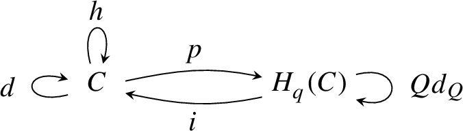
• 2nd stage. The factorization ${Q}{{d}_{{Q}}}$ is proved using the Nullstellensatz, and it is natural to study ${{d}_{{Q}}}$. The assumptions imply that ${{d}_{{Q}}}$ is exact at q, hence in a neighborhood by the HPL:

  

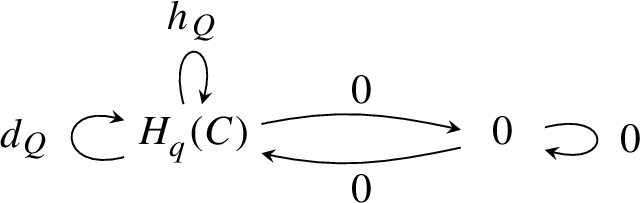
Contraction diagrams can be composed, and this gives ${H}$.

Proof

Denote by $d_q$ the differential at q, a matrix with complex entries. Such a differential always admits a contraction $h_q,i_q,p_q$ with $d_qh_qd_q = d_q$, given by matrices with complex entries. Set $\delta = d - d_q$ and

$$\begin{aligned} h = h_q(\mathbbm {1}+ \delta h_q)^{-1} \qquad i = (\mathbbm {1}+ h_q \delta )^{-1} i_q \qquad p = p_q(\mathbbm {1}+ \delta h_q)^{-1} \end{aligned}$$

Since $\delta$ has entries in $\mathbbm {C}[k]$ and vanishes at q, Cramer’s rule implies that h, i, p are matrices with entries in $\mathbbm {C}(k)$ whose denominators do not vanish at q. The HPL (13) implies that h, i, p is a contraction of d over $\mathbbm {C}(k)$ but not necessarily $dhd = d$, though this does hold at q by construction. The homologies of d and pdi coincide at each point. The assumption that $k \mapsto \dim H^{}_{k}(C)$ be constant along ${Q}=0$ near q implies that pdi vanishes along ${Q}=0$, because the dimension of the homology drops at points where $pdi \ne 0$. So Hilbert’s Nullstellensatz and irreducibility of ${Q}$ imply $pdi = {Q}{{d}_{{Q}}}$ for some matrix ${{d}_{{Q}}}$ with entries in $\mathbbm {C}(k)$ whose denominators do not vanish at q. Necessarily $({{d}_{{Q}}})^2 = 0$ and we now show that ${{d}_{{Q}q}}$ is exact. Differentiating $pdi = {Q}{{d}_{{Q}}}$ at q yields

$$\begin{aligned} p_q{\dot{d}}i_q = {\dot{{Q}}}{{d}_{{Q}q}} \end{aligned}$$

(38)

using $p_qd_q = d_qi_q = 0$. The differential $p_q{\dot{d}}i_q$ is that on $H^{}_{q}(C)$ induced by ${\dot{d}}$ which is exact by assumption, so ${\dot{{Q}}} \ne 0$ implies ${{d}_{{Q}q}}$ is exact. So it admits a homotopy ${{h}_{{Q}q}}$ with $({{h}_{{Q}q}})^2 = 0$, ${{h}_{{Q}q}}{{d}_{{Q}q}} + {{d}_{{Q}q}}{{h}_{{Q}q}} = \mathbbm {1}$. Set ${{h}_{{Q}}} = h_q'(\mathbbm {1}+ ({{d}_{{Q}}}-{{d}_{{Q}q}}) h_q')^{-1}$. By Cramer’s rule, ${{h}_{{Q}}}$ has entries in $\mathbbm {C}(k)$ whose denominators do not vanish at q, and the HPL (13) implies $({{h}_{{Q}}})^2 = 0$ and ${{h}_{{Q}}}{{d}_{{Q}}}+{{d}_{{Q}}}{{h}_{{Q}}} = \mathbbm {1}$. Define ${H}$ by (37). It is immediate that it has all the required properties. $\quad \square$

The next lemma contains more information about the composition $i {{d}_{{Q}}} p$ in Theorem 8, and shows that it induces a canonical differential on homology.

Lemma 9

(Canonical exact differential on homology). Given a regular homology point q, fix matrices $h,i,p,{d}_{{Q}},{h}_{{Q}}$ as in Theorem 8. Let k with $Q(k)=0$ be a regular homology point where these matrices are regular. Then

• $i {{d}_{{Q}}} p$ evaluated at k⁴³ induces an exact differential on $H^{}_{k}(C)$

• this differential is equivalently induced by ${\dot{d}}/{\dot{{Q}}}$ for all transversal $\xi \in T_k\mathbbm {C}^{{{m}}}$

Proof

At k we have $pdi = 0$, so the contraction h, i, p is to a complex with zero differential. The first claim follows because ${d}_{{Q}}$ is an exact differential at k. Analogous to (38) we have $p{\dot{d}}i = {\dot{{Q}}}{{d}_{{Q}}}$ at k, with derivation along $\xi$, which implies the second claim. $\quad \square$

The next lemma may be thought of as a simple special case of Theorem 8, that we will also need to construct amplitudes.

Lemma 10

(Homotopy near homology-free points). Given a complex C of finite dimensional vector spaces whose differential d has entries in $\mathbbm {C}[k]$. If $q\in \mathbbm {C}^{{{m}}}$ with $H^{}_{q}(C)=0$, then there exists a matrix h with entries in $\mathbbm {C}(k)$, whose denominators do not vanish at q, and $h^2 = 0$, $dh+hd = \mathbbm {1}$ over $\mathbbm {C}(k)$.

Proof

An application of the HPL. $\quad \square$

Next we show that Theorem 8 applies to the complexes ${\varGamma _{\text {YM}}}$, ${\varGamma _{\text {GR}}}$ and to the dgLa ${{\mathfrak {g}}}$ of Theorem 7, and we show how to transition between them via the homotopy equivalence (35b). Optimal homotopies are key in Sect. 12, to make the factorization of residues of the amplitudes manifest.

Lemma 11

(Regular homology points and homotopy equivalence). Let C, $C'$ be two complexes with homology only along ${Q}= 0$ with ${Q}$ irreducible. Suppose ${Q}(q) = 0$ and there exists a homotopy equivalence $C \leftrightarrow C'$ given by four matrices with entries in $\mathbbm {C}(k)$, regular at q. Then q is a regular homology point of C if and only if q is a regular homology point of $C'$.

Proof

We work with matrices whose entries are in $\mathbbm {C}(k)$ with denominators that do not vanish at q. If q is a regular homology point for C, apply Theorem 8 to it. Composition yields a homotopy equivalence $(H^{}_{q}(C),{Q}{d}_{{Q}}) \leftrightarrow (C',d')$, and this immediately implies that q is a regular homology point of $C'$. $\quad \square$

Lemma 12

(Single particle homology, cf. Lemma 22). The complex ${\varGamma }_{\pm h}$ has no homology if ${Q}= ad-bc \ne 0$. If ${Q}(q) = 0$ but $q \ne 0$ then

$$\begin{aligned} H^{1}_{q}({\varGamma }_{\pm h})\simeq H^{2}_{q}({\varGamma }_{\pm h}) \simeq \mathbbm {C}\qquad \qquad H^{3}_{q}({\varGamma }_{\pm h})\simeq 0 \end{aligned}$$

and every such point q is a regular homology point, so Theorem 8 applies.

Proof

It suffices to check this for one point in every orbit of the automorphism group of the cone ${Q}= 0$. Convenient are $(a,b,c,d) = (1,0,0,1)$ as well as $(a,b,c,d) = (1,0,0,0)$ and $\xi = (0,0,0,1)$. Use (19). $\quad \square$

Lemma 13

(Single particle homology). Let $h=1,2$. Take any dgLa as in Theorem 7, viewed as a vector space ${{V}}$ with differential $d^{{{V}}}$ polynomial in k. Let ${\varGamma }$ be one of ${\varGamma _{\text {YM}}}$, ${\varGamma _{\text {GR}}}$ in (34) with differential $d^{{\varGamma }}$. Let ${Q}= ad-bc$ and pick any $k \ne 0$ with ${Q}(k) = 0$. Then k is a regular homology point for both ${\varGamma }$ and ${{V}}$. Furthermore, the following maps (cf. Lemma 9) are isomorphisms

$$\begin{aligned}&H^{1}_{k}({\varGamma })\rightarrow H^{2}_{k}({\varGamma }) \text { induced by } \dot{d^{{\varGamma }}}/{\dot{{Q}}} \end{aligned}$$

(39a)

$$\begin{aligned}&H^{1}_{k}({{V}}) \rightarrow H^{2}_{k}({{V}}) \text { induced by } \dot{d^{{{V}}}}/{\dot{{Q}}} \end{aligned}$$

(39b)

and for every homotopy equivalence (35b), the associated isomorphism in homology $H^{}_{k}({\varGamma })\simeq H^{}_{k}({{V}})$ intertwines the maps (39).

Proof

By Lemma 12, k is a regular homology point of ${\varGamma }_{\pm h}$ and hence one of ${\varGamma }$. By Lemma 11 and (35b) it is also one of ${{V}}$. The maps (39) are isomorphisms because the differential in Lemma 9 is exact, and $H^{}_{k}({\varGamma })\simeq H^{}_{k}({{V}})$ are concentrated in degrees one and two. Let R, L be homotopy equivalences as in (35b). Differentiating $d^{{\varGamma }} L = L d^{{{V}}}$ along $\xi \in T_k\mathbbm {C}^{4}$ yields $\dot{d^{{\varGamma }}} L - L \dot{d^{{{V}}}} = {\dot{L}} d^{{{V}}} - d^{{\varGamma }} {\dot{L}}$; similar for R. Dividing by ${\dot{{Q}}}$, the last claim follows because the right hand side is zero on homology. $\quad \square$

Remark 10

(Inverses). Apply Theorem 8 to a regular homology point q of ${{V}}$ and suppose $h,i,p,{d}_{{Q}},{h}_{{Q}}$ are regular at k, also a regular homology point. Then the inverse of (39b) is induced by $i {h}_{{Q}}p$ evaluated at k. To see this, use ${h}_{{Q}}{d}_{{Q}}+{d}_{{Q}}{h}_{{Q}}= \mathbbm {1}$ and the fact that homology is concentrated degrees one and two. Analogously for (39a), with ${{V}}$ replaced by ${\varGamma }$.

9 Part II: Recursive Characterization

10 The Variety of Kinematically Admissible Complex Momenta

The variety for $N=n+1$ momenta is a direct product of N light cones, intersected with a codimension 4 plane that implements momentum conservation. We discuss its geometry emphasizing the Hartogs phenomenon, and list the irreducible codimension one subvarieties (prime divisors) where amplitudes can have residues. By convention, a variety need not be irreducible.

The complex light cone for the momentum

$$\begin{aligned} k = \begin{pmatrix} a &{} b \\ c &{} d \end{pmatrix} \end{aligned}$$

is the 3-dimensional irreducible quadratic variety ${V}(ad-bc) \subseteq \mathbbm {C}^4$. The singular locus is the origin and has codimension 3. Each k on the cone is non-uniquely an outer product $k = vw^T$ of vectors $v,w \in \mathbbm {C}^2$ called spinors. This is a surjective morphism of varieties

$$\begin{aligned} \mathbbm {C}^4 \rightarrow {V}(ad-bc),\qquad (v,w) \mapsto k = vw^T \end{aligned}$$

(40)

The preimage of the origin is the union of the 2-planes $v=0$ and $w=0$.

The corresponding injective map on coordinate rings $\mathbbm {C}[k]/(ad-bc) \rightarrow \mathbbm {C}[v,w]$ is given by $k \mapsto vw^T$; here k is a shorthand for four variables and v, w are shorthands for two variables each. The image consists of elements that are invariant under the algebra automorphisms $v \mapsto \lambda v$, $w \mapsto \lambda ^{-1}w$ for all $\lambda \in \mathbbm {C}^\times$. The following well-known lemma can be proved in different ways; we discuss it as preparation for Proposition 6 and Theorem 10.

Lemma 14

(Hartogs extension for the cone). A section of the structure sheaf of ${V}(ad-bc)$ on the complement of the origin $k=0$ extends uniquely to a global section, hence is the restriction of a polynomial in k to the cone.

Proof

This yields a section on the complement of $\{v = 0\} \cup \{w=0\}$ which has codimension 2. By the classical Hartogs theorem, it is the restriction of a unique element of $\mathbbm {C}[v,w]$. This element is necessarily invariant under $v \mapsto \lambda v$ and $w \mapsto \lambda ^{-1}w$ for all $\lambda \in \mathbbm {C}^\times$, hence is the image of an element of $\mathbbm {C}[k]$. $\quad \square$

Remark 11

A Hartogs-like statement such as Lemma 14 is not automatic for a singular variety. A well-known counterexample is the image of $(s,t)\in \mathbbm {C}^2 \mapsto (a,b,c,d) = (s^4,s^3t,st^3,t^4)\in \mathbbm {C}^4$. This 2-dimensional subvariety of the cone ${V}(ad-bc)$ does not satisfy Hartogs: The section of the structure sheaf given away from the origin by $b^2/a$, ac/b, bd/c, $c^2/d$ does not extend to a global section. Note that the origin has codimension 2, and it is the singular locus.

Set $k_i = ({\begin{matrix} a_i &{} b_i \\ c_i &{} d_i \end{matrix}})$ and ${Q}_i = a_id_i-b_ic_i$ and introduce 2-component vectors $v_i$ and $w_i$. We write $\mathbbm {C}[k_{1\ldots N}]$ respectively $\mathbbm {C}[v_{1\ldots N},w_{1\ldots N}]$ for the polynomial rings, each with 4N variables. The following varieties restrict N momenta to the cone and impose momentum conservation.

Definition 8

(Momenta variety). For $N \ge 3$ set:

$$\begin{aligned} I_N&= (k_1 + \ldots + k_N,{Q}_1,\ldots ,{Q}_N)&\text {an ideal in }\mathbbm {C}[k_{1\ldots N}]\\ I'_N&= (v_1w_1^T + \ldots + v_N w_N^T)&\text {an ideal in } \mathbbm {C}[v_{1\ldots N},w_{1\ldots N}] \end{aligned}$$

Then $k_i = v_iw_i^T$ defines a surjective morphism of varieties ${V}(I'_N) \rightarrow {V}(I_N)$.

Counting equations, ${V}(I_N)$ and ${V}(I'_N)$ ought to have dimensions $3N-4$ and $4N-4$ respectively. To make this rigorous one must show that the defining equations are suitably independent, a consequence of the next lemma.

Lemma 15

(Complete intersection). For $N \ge 3$ the given generators of $I_N$ and $I'_N$ are regular sequences, so the quotients are complete intersections.

Proof

Sufficient for nonzero $r_1,\ldots ,r_n$ in a polynomial ring to be a regular sequence⁴⁴ is that there exists a monomial order such that the leading monomials of $r_1,\ldots ,r_n$ are pairwise coprime.⁴⁵ We apply this as follows:

• For $I'_3$ use the degrevlex order⁴⁶ with $v_1> w_1> v_2> w_2'> v_3'> w_3> v_1'> w_1'> v_2'> w_2> v_3 > w_3'$ where, abusing notation, no dash or a dash indicate the first or second component respectively. The leading monomials of the given generators of $I'_3$ are $v_1w_1$, $v_2w_2'$, $v_3'w_3$, $v_1'w_1'$, which are coprime. The same order works for $I'_N$ with $N > 3$, by continuing the above list of monomials with $\ldots> v_4> v_4'> w_4> w_4'> \cdots> v_N> v_N'> w_N > w_N'$.

• For $I_N$ the given generators are a regular sequence iff, after eliminating $k_N$ using momentum conservation, $({Q}_1,{Q}_2,\ldots ,{Q}_{N-1}, \sum _{i \ne j,\; i,j < N} (a_i d_j - b_i c_j)$ is a regular sequence in $\mathbbm {C}[k_1,\ldots ,k_{N-1}]$. Using degrevlex with $a_1> b_1> c_1> d_1> a_2> b_2> c_2> d_2> \cdots> a_{N-1}> b_{N-1}> c_{N-1} > d_{N-1}$, the leading monomials are $b_1c_1$, $b_2c_2$, ..., $b_{N-1}c_{N-1}$, $a_2d_1$, which are coprime. $\quad \square$

Proposition 6

(Hartogs extension for the momenta variety). If $N \ge 3$ and $X = {V}(I_N)$ or $X = {V}(I'_N)$, and if $Y \subseteq X$ is a Zariski closed subset of codimension $\ge 2$, then restriction defines an isomorphism

$$\begin{aligned} {\mathcal {O}}_X(X) \simeq {\mathcal {O}}_X(X-Y) \end{aligned}$$

(41)

That is, every section of the structure sheaf away from Y extends uniquely to a global section, and is therefore the restriction of a polynomial to X.

Proof

A complete intersection is $S_2$ which implies Hartogs. More in detail, a complete intersection, meaning a polynomial ring modulo a regular sequence, is a local complete intersection, meaning all its local rings are complete intersections. Hence it is a Gorenstein ring and a Cohen–Macaulay ring by [27, Theorems 21.3 and 18.1], and it has the property $S_k$ of Serre for all k, see [27, Section 23]. Equation (41) now follows from [28, Proposition 1.11]. The elements of ${\mathcal {O}}_X(X)$ are well-known to be restrictions of polynomials. $\quad \square$

We now discuss further geometric properties of these ideals, first for $N \ge 4$. The $N=3$ special case is discussed later.

Proposition 7

(Primality). If $N \ge 4$ then $I_N$ and $I'_N$ are prime ideals.

Proof

This follows from Lemma 29 in “Appendix B”, with $n = N$ and $f = 0$, and the dummy choices $d = 1$ and ${{\mathfrak {p}}}= (x) \subseteq \mathbbm {C}[x]$ the maximal ideal. $\quad \square$

Lemma 16

(Singular loci). For $N \ge 4$ the singular loci are:

• ${V}(I_N)$: Points where $k_i=0$ for at least one $i = 1\ldots N$, and points where all the $k_1,\ldots ,k_N$ are contained in one line in $\mathbbm {C}^4$. Codimension 3.

• ${V}(I'_N)$: Points where all the $v_1w_1^T,\ldots ,v_Nw_N^T$ are contained in one line in $\mathbbm {C}^4$. Codimension $2N-5 \ge 3$.

Proof

Consider say ${V}(I_N)$, $N\ge 4$. Abbreviate $dQ_i = (d_i,-c_i,-b_i,a_i)$. The Jacobian of the list of generators of $I_N$ has the block structure

and is surjective iff $dQ_i \ne 0$ for all i and $\sum _i \ker (d Q_i) = \mathbbm {C}^4$, hence iff $k_i \ne 0$ for all i and at least two $k_i$ are linearly independent. This is the non-singular locus by the Jacobian criterion and primality of $I_N$ in Proposition 7, by which $I_N$ is the ideal of ${V}(I_N)$, see [29, Section I.5]. Similar for ${V}(I_N')$. $\quad \square$

Lemma 17

(Normality). If $N \ge 4$ then the quotient rings of $I_N$ and $I'_N$ are normal Noetherian domains.

Proof

Normality follows from Serre’s criterion, because the ring is a complete intersection by Lemma 15 hence $S_2$, and the singular locus has codimension $>1$ by Lemma 16. It is an integral domain by Proposition 7. $\quad \square$

Lemma 18

(Preimage). If $N \ge 4$, then under ${V}(I'_N) \rightarrow {V}(I_N)$ the preimage of every Zariski closed subset of codimension $\ge 2$ has codimension $\ge 2$.

Proof

Let $S \subseteq {V}(I'_N)$ be the union of (a) the singular locus, (b) the preimage of the singular locus of ${V}(I_N)$ under the map ${V}(I'_N) \rightarrow {V}(I_N)$, and (c) all points where the Jacobian of this map does not have full rank $3N-4$. One checks that (b) contains (a) and (c). So S has codimension 2. Consider now the claim. If the preimage does not have codimension $\ge 2$, then it has an irreducible component with codimension $\le 1$, this component has (since its singular locus is proper and closed) at least one non-singular point not in S, but then by a local analysis its image has codimension $\le 1$, a contradiction. $\quad \square$

We now discuss the special case $N=3$. Two remarks:

• The singular locus of ${V}(I_3)$ has codimension one, as one can check.

• Lemma 18 fails for ${V}(I'_3) \rightarrow {V}(I_3)$, because $\{ k_1=0 \}$ has codimension 2 but its preimage $\{ v_1 = 0 \} \cup \{ w_1 = 0 \}$ only has codimension 1.

Proposition 8

(Prime decomposition for $N=3$). The ideal $I_3$ is radical but not prime, instead $I_3 = I^+ \cap I^-$ for two prime ideals $I^{\pm } \subseteq \mathbbm {C}[k_{1\ldots 3}]$:

$$\begin{aligned} I^+&= \big (k_1 + k_2 + k_3,\, \text {all maximal minors of the } 2 \times 6 \text { matrix } (k_1\,k_2\,k_3)\big )\\ I^-&= \big (k_1 + k_2 + k_3,\, \text {all maximal minors of the } 2 \times 6 \text { matrix }(k_1^T\,k_2^T\,k_3^T)\big ) \end{aligned}$$

So ${V}(I_3) = {V}(I^+) \cup {V}(I^-)$, where ${V}(I^+)$ are all points of the form $k_i = vw_i^{T}$ with $w_1+w_2+w_3=0$, and ${V}(I^-)$ are all points of the form $k_i = v_iw^{T}$ with $v_1+v_2+v_3=0$. The ring $\mathbbm {C}[k_{1\ldots 3}]/I^\pm$ is Cohen–Macaulay.

Proof

Equation $I_3 = I^+ \cap I^-$ may be rigorously checked using Gröbner bases. For example, the following Macaulay2 [30] code does just that (see Remark 12):

For the primality of $I^\pm$ we include two independent proofs:

• The ring $\mathbbm {C}[k_{1\ldots 3}]/I^\pm$ is isomorphic to the coordinate ring of the determinantal variety of $2 \times 4$ matrices of rank $<2$, hence an integral domain and Cohen–Macaulay by Corollary 2.8 and Theorem 2.10 in [31].

• It suffices to check that $I^+$ is the kernel of the ring map

  $$\begin{aligned} \mathbbm {C}[k_{1\ldots 3}] \rightarrow \mathbbm {C}[v,w_{1\ldots 3}]/(w_1+w_2+w_3),\quad k_i \mapsto vw_i^T \end{aligned}$$

  because then $\mathbbm {C}[k_{1\ldots 3}]/I^+$ is isomorphic to a subring of an integral domain, hence itself an integral domain. To check that $I^+$ is indeed the kernel, one can use Gröbner bases, for example, the following Macaulay2 code:

  

Every intersection of prime ideals is radical, therefore $I_3$ is radical. $\quad \square$

Note that⁴⁷$I^+ \cap I^- \ne I^+I^-$.

Remark 12

Gröbner bases software such as Macaulay2 [30] may be used to calculate, in particular, intersections of ideals and kernels of ring maps. In these cases, results over $\mathbbm {Q}$ are also valid over $\mathbbm {C}$ in the following sense: Given two ideals in a polynomial ring $\mathbbm {C}[x_1,\ldots ,x_d]$, specified by generating polynomials in $\mathbbm {Q}[x_1,\ldots ,x_d]$, then if one computes their intersection in $\mathbbm {Q}[x_1,\ldots ,x_d]$ and obtains a set of generators, those are also generators of the intersection of the original ideals in $\mathbbm {C}[x_1,\ldots ,x_d]$. Similar for the kernel of a ring map.

Lemma 19

(Injective ring map). For $N \ge 3$ the assignment $k_i \mapsto v_i w_i^T$ induces an injective ring map $\mathbbm {C}[k_{1\ldots N}]/I_N \rightarrow \mathbbm {C}[v_{1\ldots N},w_{1\ldots N}]/I'_N$.

Proof

Every element in the kernel of $\mathbbm {C}[k_{1\ldots N}] \rightarrow \mathbbm {C}[v_{1\ldots N},w_{1\ldots N}]/I'_N$ vanishes on ${V}(I_N)$, since ${V}(I'_N) \rightarrow {V}(I_N)$ is surjective. Therefore it is in the radical $\sqrt{I_N}$ by the Nullstellensatz. But $I_N$ is radical, $\sqrt{I_N} = I_N$ (if $N=3$ see Proposition 8, if $N \ge 4$ see Proposition 7 and recall that prime implies radical). Hence the kernel is contained in $I_N$. Conversely, $I_N$ is in the kernel. $\quad \square$

The remainder of this section concerns subvarieties that, in the case of amplitudes, are the geometric loci where internal momenta go on-shell.

Definition 9

(Internal momenta). Given $N \ge 4$, an internal momentum is a subset $J \subseteq \{1,\ldots ,N\}$ with $2 \le |J| \le N-2$ and we denote

$$\begin{aligned} k_J&= \textstyle \sum _{i \in J} k_i\\ {Q}_J&= \det k_J \end{aligned}$$

in $\mathbbm {C}[k_{1\ldots N}]/I_N$. Note that $k_J = -k_{J^c}$ and ${Q}_J = {Q}_{J^c}$ and ${Q}_J$ is nonzero on an open dense subset of ${V}(I_N)$. The integer N is always taken from context.

Definition 10

(Prime divisors). Set ${\mathfrak {P}}_3 = \{\}$. For $N \ge 4$ set

$$\begin{aligned} {\mathfrak {P}}_N = \bigg \{ \;{{\mathfrak {p}}}\subseteq \mathbbm {C}[k_{1\ldots N}]/I_N\;\bigg |\; \begin{aligned}&\text {there is an internal }J \text { such that }{{\mathfrak {p}}}\text { is a minimal}\\&\text {prime ideal over the principal ideal }({Q}_J) \end{aligned} \bigg \} \end{aligned}$$

This is a finite set by a theorem of Noether, and each ${{\mathfrak {p}}}$ has height one by Krull’s principal ideal theorem. So ${\mathfrak {P}}_N$ is a finite set of prime divisors.

Theorem 9

(Classification of prime divisors). For $N = 4$ one has $|{\mathfrak {P}}_4|=8$ prime divisors, the following and their inequivalent permutations:⁴⁸

If $N \ge 5$ then every prime divisor ${{\mathfrak {p}}}\in {\mathfrak {P}}_N$ lies over a unique $({Q}_J)$:

• If J and $J^c$ both have at least three elements, then $({Q}_J)$ is itself prime.

• For $i \ne j$ there are exactly two minimal primes over $({Q}_{ij})$, namely ${{\mathfrak {p}}}_{ij}^+$ and ${{\mathfrak {p}}}_{ij}^-$ generated by the maximal minors of $(k_i\,k_j)$ respectively $(k_i^T\,k_j^T)$.

Remark 13

Recall that, in a commutative unital ring, if $\{{{\mathfrak {p}}}_\ell \}$ is a finite set of prime ideals with the property that for every index m one has $\cap _{\ell : \ell \ne m} {{\mathfrak {p}}}_\ell \not \subseteq {{\mathfrak {p}}}_{m}$, then $\{{{\mathfrak {p}}}_\ell \}$ is exactly the set of minimal primes over the radical ideal $\cap _\ell {{\mathfrak {p}}}_\ell$.⁴⁹

Proof

Distinguish two cases:

• $N=4$: Up to permutation, it suffices to show that the minimal primes over $({Q}_{12})$ are $\{{{\mathfrak {p}}}_{++++}, {{\mathfrak {p}}}_{----}, {{\mathfrak {p}}}_{++--}, {{\mathfrak {p}}}_{--++}\}$. By the same logic used to prove primality of $I^\pm$ in Proposition 8, ${{\mathfrak {p}}}_{++++}$ is prime because, by a Gröbner bases calculation (see Remark 12), it is the kernel of the ring map

  $$\begin{aligned} \mathbbm {C}[k_{1\ldots 4}]/I_4&\rightarrow \mathbbm {C}[v,w_{1\ldots 4}]/(w_1+w_2+w_3+w_4)\\ k_i&\mapsto vw_i^T \end{aligned}$$

  and ${{\mathfrak {p}}}_{++--}$ is prime because it is the kernel of the ring map

  $$\begin{aligned} \mathbbm {C}[k_{1\ldots 4}]/I_4&\rightarrow \mathbbm {C}[w_1,w_2,v_3,v_4]\\ k_{1\ldots 4}&\mapsto ((v_3+v_4)w_1^T,(v_3+v_4)w_2^T,-v_3(w_1^T+w_2^T),-v_4(w_1^T+w_2^T)) \end{aligned}$$

  Analogously for ${{\mathfrak {p}}}_{----}$ and ${{\mathfrak {p}}}_{--++}$. By a Gröbner bases calculation, the intersection of these four ideals is $({Q}_{12})$ and none of them is redundant. Hence we are done by Remark 13.

• $N \ge 5$: We use “Appendix B”. We are interested in primality, but we discuss geometric irreducibility first. Suppose $|J|, |J^c| \ge 3$. We have

  $$\begin{aligned} {V}({Q}_J)&\simeq {V}(I_{|J| + 1}) \times _{{{\mathbbm {C}^{4}}}} {\text {Cone}}^{|J^c|} \\ {V}({{\mathfrak {p}}}_{ij}^{\pm })&\simeq {V}(I^{\pm }) \times _{{{\mathbbm {C}^{4}}}} {\text {Cone}}^{N-2} \end{aligned}$$

  where the first fiber product is defined using

  $$\begin{aligned} {V}(I_{|J|+1}) \xrightarrow {\;\;((k_i)_{i \in J},k) \mapsto k \;\;} {{\mathbbm {C}^{4}}} \xleftarrow {\;\;(k_i)_{i \notin J} \mapsto \sum _{i \notin J} k_i \;\;} {\text {Cone}}^{|J^c|} \end{aligned}$$

  and the second is analogous. Lemma 28 now implies that ${V}({Q}_J)$ and ${V}({{\mathfrak {p}}}_{ij}^{\pm })$ are irreducible, since ${V}(I_{|J|+1})$ and ${V}(I^{\pm })$ are irreducible. Writing out the same isomorphisms at the level of ideals, Lemma 29 implies that $({Q}_J)$ and ${{\mathfrak {p}}}_{ij}^{\pm }$ are prime, since $I_{|J|+1}$ and $I^{\pm }$ are prime, where still $|J|,|J^c| \ge 3$. So, $({Q}_J)$ is minimal if $|J|,|J^c| \ge 3$, and by Remark 13 it now suffices to show that ${{\mathfrak {p}}}_{ij}^{\pm } \not \subseteq {{\mathfrak {p}}}_{ij}^{\mp }$, which is clear, and that ${{\mathfrak {p}}}_{ij}^+ \cap {{\mathfrak {p}}}_{ij}^- = \sqrt{({Q}_{ij})}$.⁵⁰ The last inclusion follows from the Nullstellensatz and the geometric equality ${V}({{\mathfrak {p}}}_{ij}^+) \cup {V}({{\mathfrak {p}}}_{ij}^-) = {V}({Q}_{ij})$. Inclusion $\subseteq$ in this geometric equality is trivial, inclusion $\supseteq$ follows from ${V}(I_3) = {V}(I^+) \cup {V}(I^-)$ in Proposition 8. $\quad \square$

Definition 11

(The P and Z subsets). For $N \ge 4$ set

$$\begin{aligned} P_N&= \textstyle \bigcup _{{{\mathfrak {p}}}\in {\mathfrak {P}}_N} {V}({{\mathfrak {p}}})&Z_N&= \textstyle \bigcup _{{{\mathfrak {p}}}, {{\mathfrak {q}}}\in {\mathfrak {P}}_N:\; {{\mathfrak {p}}}\ne {{\mathfrak {q}}}} {V}({{\mathfrak {p}}}) \cap {V}({{\mathfrak {q}}}) \end{aligned}$$

which are closed subsets of ${V}(I_N)$. Let

$$\begin{aligned} P_3 = Z_3 = \{k_1 = 0\} \cup \{k_2 = 0\} \cup \{k_3 = 0\} \end{aligned}$$

viewed as closed subsets of one of ${V}(I^{\pm })$.

Note that $P_N$ is equivalently the union of all ${V}({Q}_J)$, but there is no analogous definition of $Z_N$. Note that $Z_3$ has codimension two. The role of the subvariety $Z = Z_N$ is informally discussed in Sect. 1.

Proposition 9

(Good properties away from Z). Let $N \ge 4$. Then the subset $Z_N \subseteq {V}(I_N)$ has codimension $\ge 2$. In the complement $Z_N^c$:

• We have $k_i \ne 0$ for all $i = 1,\ldots ,N$ and $k_J\ne 0$ for all internal J. The $k_i \in \mathbbm {C}^4$ are pairwise linearly independent.

• The variety ${V}(I_N)$ is smooth of dimension $3N-4$.

• ${Q}_J$ has nonzero derivative tangent to ${V}(I_N)$, for all internal J. In particular ${V}({Q}_J)$ is smooth and has codimension one.

• $P_N$ is a smooth codimension one subvariety. If a point in ${V}({{\mathfrak {p}}})$ also lies in ${V}({Q}_J)$, then necessarily ${{\mathfrak {p}}}\supseteq ({Q}_J)$ and locally ${V}({{\mathfrak {p}}}) \simeq {V}({Q}_J)$.

Proof

Every intersection of two distinct irreducible codimension one subvarieties has codimension $\ge 2$, so $Z_N$ has. For $Z_N^c$, several claims follow from ${V}({{\mathfrak {p}}}_{ij}^+) \cap {V}({{\mathfrak {p}}}_{ij}^-)$ which contains all points with $k_i = 0$; all points with $k_{\{i,j\}}=k_i+k_j=0$; all points where $k_i$ and $k_j$ are linearly dependent. Points where $k_J=0$ with $|J|,|J^c| \ge 3$ are in ${V}({Q}_J) \cap {V}({Q}_{J\cup \{i\}})\subseteq Z_N$ for all $i \notin J$. Smoothness of ${V}(I_N)$ by Lemma 16. The tangent derivative of ${Q}_J=\det k_J$ is nonzero since $k_J \ne 0$ and the Jacobian of $Z_N^c \rightarrow \mathbbm {C}^4, (k_1,\ldots ,k_N) \mapsto k_J$ has rank four, which one sees using pairwise linear independence of the $k_i$. Every point of $P_N\cap Z_N^c$ lies in a unique ${V}({{\mathfrak {p}}})$, hence in ${V}({Q}_J)$ iff ${{\mathfrak {p}}}\supseteq ({Q}_J)$. $\quad \square$

11 The Helicity Sheaf for One Particle

Here we discuss certain rank one sheaves on the cone $X = {V}(ad-bc)$ and show how they arise as the homology of the complexes ${\varGamma }_{\pm h}$. Their fiber over each nonzero momentum is the space of polarizations for a gluon without color when $h=1$ (YM), or a graviton when $h=2$ (GR), with helicity $+$ or −.

In this section we denote $R = \mathbbm {C}[k]/(ad-bc)$ and $k = ({\begin{matrix} a &{} b \\ c &{} d \end{matrix}})$. It is convenient to set $k^+ = k$ and $k^- = k^T$. For every half-integer $h \ge 0$ let

$$\begin{aligned} S^{2h} k^{+} = \left( {\begin{matrix} a^{2h}&{}\cdots &{} b^{2h} \\ \vdots &{} \ddots &{} \vdots \\ c^{2h}&{}\cdots &{} d^{2h} \end{matrix}}\right) \end{aligned}$$

(42)

be the $(2h+1)\times (2h+1)$ matrix with entries in R where multiplication of an entry by ${\frac{b}{a}}={\frac{d}{c}}$ gives the next entry to the right, multiplication by ${\frac{c}{a}}={\frac{d}{b}}$ gives the next entry below. It is the symmetrized Kronecker product of matrices,

$$\begin{aligned} S^{2h}k^{+} \in {{\,\mathrm{End}\,}}_R(S^{2h}R^2) \end{aligned}$$

using $S^{2h}R^2 \simeq R^{2h+1}$. The matrix $S^{2h}k^{-}$ is the transpose.

Remark 14

The Lorentz group acts as graded ring automorphisms on R. The degree subspaces of R are irreducible, $R \simeq \bigoplus _h {(}h,h{)}$ where a $\mathbbm {C}$-basis of ${(}h,h{)}$ is given by the entries of (42). There is a category of graded R-modules whose objects M are also Lorentz modules with Lorentz equivariant scalar multiplication $R \times M \rightarrow M$, and whose morphisms are Lorentz equivariant. In this category, $S^{2h}k^+$ is the unique morphism $R \otimes {(}0,h{)} \rightarrow R \otimes {(}h,0{)}$ of degree 2h, up to normalization. Hence its image is also a Lorentz module, and its degree subspaces are seen to be irreducible,⁵¹${{\,\mathrm{im}\,}}S^{2h} k^+ \simeq \bigoplus _p {(}p,p+h{)}$.

Remark 15

(Momentum conservation). Consider the involutive graded ring automorphism on R given by $k \mapsto -k$. It induces an endofunctor on R-modules that we call ${{\,\mathrm{flip}\,}}$. For every graded module M one canonically has ${{\,\mathrm{flip}\,}}(M) \simeq M$ as modules, so ${{\,\mathrm{flip}\,}}$ is vacuous in this sense. However ${{\,\mathrm{flip}\,}}$ could be used in various places to make momentum conservation – equivariance under the translation group – manifest. For instance, in equation (43) below one could apply ${{\,\mathrm{flip}\,}}$ to either of the two input factors, so that the isomorphism holds with the trivial action of the translation group on ${\mathcal {O}}_X$. To simplify the notation, we leave it to the reader to insert ${{\,\mathrm{flip}\,}}$ in the right places.

We use the following notation:   $\smash {\widetilde{}}$   is the module to sheaf functor; every nonzero $f\in R$ defines a standard open $D_f = \{ x \in X \mid f(x) \ne 0 \}$; the localization $R_f$ is its coordinate ring. See “Appendix A”.

Remark 16

(Local factorization of momenta) We use the standard open cover $X-0= D_a \cup D_b \cup D_c \cup D_d$. On each patch there is a factorization $k = v w^T$. For example, on $D_a$ one can use $v=({\begin{matrix}a\\ c\end{matrix}})$, $w=({\begin{matrix}1\\ b/a\end{matrix}})$ with all entries in $R_a$ and they are unique up to replacing v, w by $\lambda v, \lambda ^{-1}w$ for any invertible $\lambda \in R_a$.

Lemma 20

(Locally free of rank one). The sheaf $({{\,\mathrm{im}\,}}S^{2h}k^{\pm })\,\,\smash {\widetilde{}}\,\,|_{X-0}$ is locally free of rank one.⁵²

Proof

On each standard open set in Remark 16, an isomorphism ${{\,\mathrm{im}\,}}(S^{2h}k^\pm )_f \simeq {{\,\mathrm{im}\,}}( (S^{2h}k^\pm )_f )\rightarrow R_f$ is given by $v^{\otimes 2h} \mapsto 1$ and $w^{\otimes 2h} \mapsto 1$ respectively. $\quad \square$

Lemma 21

(Inverse sheaf). There is a canonical isomorphism of sheaves

$$\begin{aligned} ({{\,\mathrm{im}\,}}S^{2h}k^+)\,\,\smash {\widetilde{}}\,\,|_{X-0} \otimes ({{\,\mathrm{im}\,}}S^{2h}k^-)\,\,\smash {\widetilde{}}\,\,|_{X-0} \;\simeq \; {\mathcal {O}}_X|_{X-0} \end{aligned}$$

(43)

given on each standard open in Remark 16 by $v^{\otimes 2h}\otimes w^{\otimes 2h} \mapsto 1$.

Proof

The map is well-defined on standard open sets by Remark 16, and compatible on overlaps. $\quad \square$

Definition 12

Let C be a complex of vector spaces depending parametrically on $k\in \mathbbm {C}^4$, whose differential is a matrix with entries in $\mathbbm {C}[k]$. By regarding the matrix entries as elements of R, these matrices define a complex of free R-modules that we denote by ${C^{R}}$.

For example, if this definition is applied to ${\varGamma }_{2}$, then ${\varGamma ^{R}_{2}}$ is a complex of free R-modules $0\rightarrow R^{5} \rightarrow R^{8} \rightarrow R^{3}\rightarrow 0$ with differential (19).

Lemma 22

(Single particle homology, cf. Lemma 12). The homology $H^j({\varGamma ^{R}_{\pm h}})\,\,\smash {\widetilde{}}\,\,|_{X-0}$ is locally free of rank one if $j=1,2$ and zero otherwise. There are canonical isomorphisms of locally free rank one sheaves

$$\begin{aligned} ({{\,\mathrm{im}\,}}S^{2h}k^\pm )\,\,\smash {\widetilde{}}\,\,|_{X-0} \;\simeq \; H^1({\varGamma ^{R}_{\pm h}})\,\,\smash {\widetilde{}}\,\,|_{X-0} \;\simeq \; H^2({\varGamma ^{R}_{\pm h}})\,\,\smash {\widetilde{}}\,\,|_{X-0} \end{aligned}$$

(44)

The first is induced by $v^{\otimes 2h}\mapsto v^{\otimes 2h}$ respectively $w^{\otimes 2h}\mapsto w^{\otimes 2h}$ on each standard open set in Remark 16. The second is induced by the canonical map (39a).

Proof

For the locally free claim use Theorem 8, which for every point on $X-0$ produces a local trivialization.⁵³ The first map in (44) is globally well-defined, in particular independent of the local factorization $k=vw^T$, and $v^{\otimes 2h}$ represents a nonzero element in homology because $k^- \epsilon v = 0$ and because $H^1$ is a kernel. For the second map, see also Lemma 9 and Remark 10. $\quad \square$

12 The Helicity Sheaf

We show that a certain rank one sheaf $\smash {\widetilde{M}}$ on ${V}(I_N)$ satisfies a variant of Hartogs extension if $N \ge 4$, while for $N=3$ there is local cohomology along $Z_3$. These results are used respectively to prove the uniqueness of amplitudes and to define the 2-to-1 amplitude, in the next section.

In this section, R denotes one of $R^\pm$ if $N=3$ respectively $R_N$ if $N \ge 4$, and X denotes one of $X^\pm$ if $N=3$ respectively $X_N$ if $N \ge 4$. Here,

$$\begin{aligned} R^{\pm }&= \mathbbm {C}[k_{1\ldots 3}]/I^{\pm }&X^{\pm }&= {V}(I^{\pm })\\ R_N&= \mathbbm {C}[k_{1\ldots N}]/I_N&X_N&= {V}(I_N) \end{aligned}$$

Recall that X is irreducible, R is its coordinate ring, and R is Cohen–Macaulay, see Sect. 8. Set $k_i = ({\begin{matrix} a_i &{} b_i \\ c_i &{} d_i \end{matrix}})$ and define the matrices $S^{2h}k_i^{\pm }$ as in Sect. 9.

Definition 13

(The helicity module M). For every integer $N\ge 3$, every half-integer $h \ge 0$ and every N-tuple of signs $\sigma \in \{-,+\}^N$:

• If $N \ge 4$, let $M_h^\sigma \subseteq R^{((2h+1)^N)}$ be the finitely generated R-module that is the image of the following Kronecker product of matrices:

  $$\begin{aligned} S^{2h}k_1^{\sigma _1} \otimes \cdots \otimes S^{2h}k_N^{\sigma _N} \end{aligned}$$

  (45)

• If $N=3$, make the same definition over $R^\pm$, denoted $M^{\pm ,\sigma }_h$.

We often use the shorthand M. Note that the module M inherits a grading from the ambient free module, and as such is generated in degree 2hN.

Remark 17

Analogous to Remark 14, here the Lorentz group acts as automorphisms on R separately on each $k_i$, preserving $k_1 + \ldots + k_N = 0$. Hence M is also a Lorentz module.

By definition of the   $\smash {\widetilde{}}$   functor, $\smash {\widetilde{M}}(X) \simeq M$, see “Appendix A”.

Theorem 10

(Hartogs extension for the helicity sheaf). If $N \ge 4$ then for all Zariski closed subsets $Y \subseteq X$ of codimension $\ge 2$, the restriction map from X to $X-Y$ induces an isomorphism

$$\begin{aligned} M \simeq \smash {\widetilde{M}}(X-Y) \end{aligned}$$

Proof

This proof contains elements of the proof of Lemma 14 and uses spinors. Let $R' = \mathbbm {C}[v_{1\ldots N},w_{1\ldots N}]/I'_N$. Recall $\phi : R \rightarrow R'$, $k_i \mapsto v_iw_i^T$ the injective ring map in Lemma 19. Let $L = (2h+1)^N$ and let K be the $L \times L$ matrix (45). The definition of $\phi$ implies a matrix factorization $\phi (K) = IS$ where I is a column vector and S is a row vector with entries in $R'$. And $I: R' \rightarrow R'^L$ is injective since $R'$ is an integral domain. Note that $\phi ^L K = IS \phi ^L$ hence the injectivity of $\phi$ and I yield a well-defined injective $\phi$-linear map⁵⁴$\alpha : M \rightarrow R'$, $Kx \mapsto S \phi ^L x$. The image of $\alpha$ is precisely the $\mathbbm {C}$-subspace of all $y\in R'$ that for all $(\lambda _1,\ldots ,\lambda _N) \in (\mathbbm {C}^\times )^{N}$ transform like

$$\begin{aligned} y \mapsto {\lambda _1^{-2h\sigma _1 }\cdots \lambda _N^{-2h\sigma _N } y} \end{aligned}$$

(46)

under the algebra automorphism of $R'$ given by $v_i \mapsto \lambda _i v_i$ and $w_i \mapsto \lambda _i^{-1} w_i$. Set $X' = {V}(I'_N)$. Let $Y'$ be the preimage of Y under $X' \rightarrow X$. We have the following commutative diagram, where $\rho$ and $\rho '$ are restriction maps, and $\beta = \smash {\widetilde{\alpha }}(X-Y)$ is induced by $\alpha$ and is injective⁵⁵:

Crucially, $\rho '$ is bijective by Proposition 6 for $X'$ and because $Y'$ has codimension $\ge 2$ by Lemma 18 and $N \ge 4$. The diagram implies that $\rho$ is injective. The following $(\mathbbm {C}^{\times })^{N}$-actions on the spaces in the diagram make all arrows equivariant: act trivially on the two spaces on the left, act on $R'$ as defined earlier. This makes sense because $Y'$ is $(\mathbbm {C}^{\times })^{N}$-invariant. Hence elements in the image of $(\rho ')^{-1} \beta$ transform like (46) and are contained in the image of $\alpha$. This implies that $\rho$ is also surjective. $\quad \square$

Lemma 18 fails for $N = 3$ and in fact then there is a different result. Theorem 11 and Lemma 23 below make precise an argument in the literature [5, Section 2.3], and construct the 2-to-1 amplitudes for YM and GR. The codimension two subset $Z_3$ in Definition 11 was chosen with this application in mind. There is an analogous proposition for $X^-$.

Theorem 11

(Hartogs failure for the helicity sheaf in $N=3$). For all $\sigma \in \{-,+\}^3$, restriction induces an injection of graded $R^+$-modules⁵⁶

$$\begin{aligned} M_h^{+,\sigma } \hookrightarrow \smash {\widetilde{M_h^{+,\sigma }}}(X^+-Z_3) \end{aligned}$$

The module on the left is generated in degree 6h. The module on the right is generated in degree 6h if $\sigma = {+}{+}{+},\, {-}{-}{-}$ and in degree 4h if $\sigma = {+}{+}{-},\, {+}{-}{-}$. As a Lorentz representation, see Remark 17, the degree 4h subspace is:

$$\begin{aligned} {+}{+}{-}\;\;:\;\; S^{2h} ({(}0,\tfrac{1}{2}{)} \oplus {(}0,\tfrac{1}{2}{)}) \qquad \qquad {+}{-}{-}\;\;:\;\; S^{2h} {(}\tfrac{1}{2},0{)} \end{aligned}$$

(48)

Analogous for permutations of $\sigma$.

Proof

This proof follows closely that of Theorem 10. Here $M = M_h^{+,\sigma }$ and $X = X^+$ and $R' = \mathbbm {C}[v,w_1,w_2,w_3]/(w_1+w_2+w_3)$ an integral domain and $\phi : R^+ \rightarrow R'$, $k_i \mapsto vw_i^T$ an injective ring map. The map $\alpha : M \rightarrow R'$, defined analogously to the one in the proof of Theorem 10, is injective. The image of $\alpha$ is the $\mathbbm {C}$-subspace of $R'$ spanned by all elements of the schematic form⁵⁷

$$\begin{aligned} v^{n_1+n_2+n_3+m_1^- + m_2^- + m_3^-} w_1^{n_1 + m_1^+} w_2^{n_2 + m_2^+} w_3^{n_3 + m_3^+} \end{aligned}$$

(49)

for all $n_1,n_2,n_3 \in \mathbbm {Z}_{\ge 0}$. Here $m_i^\pm = h(1\pm \sigma _i)\in \{0,2h\}$. The preimage of $Y=Z_3$ under $X' \rightarrow X$ is $Y' = \{v=0\} \cup \{w_1=0\} \cup \{w_2 = 0\} \cup \{w_3 = 0\}$ and has codimension 2. We again have the commutative diagram (47), in particular Hartogs on $X' \simeq \mathbbm {C}^6$ implies that $\rho '$ is bijective. The following are equal:

• (1) The set of all $y\in R'$ that for $\lambda \in \mathbbm {C}^\times$ transform like $y \mapsto \lambda ^{-2h(\sigma _1+\sigma _2+\sigma _3)}y$ under the algebra automorphism $v \mapsto \lambda v$ and $w_i \mapsto \lambda ^{-1} w_i$.

• (2) The $\mathbbm {C}$-subspace of $R'$ spanned by the elements (49) however allowing all $n_1,n_2,n_3 \in \mathbbm {Z}$ that give four nonnegative exponents. That is, all elements of the form $v^{n - 2h(\sigma _1+\sigma _2+\sigma _3)} w^n$ with $n \ge 0$ and $n \ge 2h(\sigma _1+\sigma _2+\sigma _3)$ where w is schematic for all components of $w_1,w_2,w_3$.

• (3) The image of $(\rho ')^{-1}\beta$.

Here $\text {(1)} \subseteq \text {(2)}$ is clear, $\text {(2)} \subseteq \text {(3)}$ is proved using the fact that on $X-Z_3$ one can locally factor⁵⁸$k_i = v w_i^T$, and $\text {(3)} \subseteq \text {(1)}$ by $\mathbbm {C}^\times$-equivariance of (47). Using (2), the lowest degree pieces in the image of $(\rho ')^{-1}\beta$ are all elements $w^{6h}$ for ${+}{+}{+}$, $w^{2h}$ for ${+}{+}{-}$, $v^{2h}$ for ${+}{-}{-}$, $v^{6h}$ for ${-}{-}{-}$. For ${+}{+}{-}$ and ${+}{-}{-}$ this is below the lowest degree of the image of $\alpha$, by 4h in $R'$-degree, 2h in $R^+$-degree. Given the quotient by $w_1+w_2+w_3$, the Lorentz modules of all $w^{2h}$ respectively $v^{2h}$ are as claimed using the natural Lorentz action on $R'$, since (47) is Lorentz equivariant using the Lorentz module structure on M in Remark 17. $\quad \square$

Remark 18

Note that $S^{2h} ({(}0,\tfrac{1}{2}{)} \oplus {(}0,\tfrac{1}{2}{)}) \simeq \bigoplus _{m+n=2h}S^{m}{(}0,\tfrac{1}{2}{)}\otimes S^{n}{(}0,\tfrac{1}{2}{)}$ contains the trivial representation exactly once if 2h is even, never if 2h is odd. The trivial representation never appears in $S^{2h} {(}\tfrac{1}{2},0{)} \simeq {(}h,0{)}$ if $h>0$.

Lemma 23

(2-to-1 amplitude to-be). If $h \in \mathbbm {Z}_{\ge 0}$ then $\smash {\widetilde{M_h^{+,++-}}}(X^+-Z_3)$ contains a unique Lorentz invariant element of degree 4h, up to normalization. It is given for any local factorization $k_i = v w_i^T$ with $w_1 + w_2 + w_3 = 0$ by

$$\begin{aligned} (w_1^T \epsilon w_2)^h\;v^{\otimes 2h} \otimes v^{\otimes 2h} \otimes w_3^{\otimes 2h} \end{aligned}$$

(50a)

where $\epsilon = ({\begin{matrix} 0 &{} 1 \\ -1 &{} 0 \end{matrix}})$. Analogous element in $\widetilde{M_h^{-,--+}}(X^--Z_3)$ using $k_i = v_iw^T$:

$$\begin{aligned} (v_1^T \epsilon v_2)^h\;w^{\otimes 2h} \otimes w^{\otimes 2h} \otimes v_3^{\otimes 2h} \end{aligned}$$

(50b)

Analogous for $\smash {\widetilde{M^{+,\sigma }}}$ if $\sigma$ has two plus, and for $\smash {\widetilde{M^{-,\sigma }}}$ if $\sigma$ has two minus.

Proof

The expression is independent of the local factorization, so we get a section. It is Lorentz invariant. It is unique by Remark 18. $\quad \square$

Next we define a sheaf $\smash {\widetilde{C}}$, isomorphic to $\smash {\widetilde{M}}$ on the complement of a codimension two subset. It will be used to reinterpret the amplitudes in Definition 6 as sections of a sheaf, in Sect. 11.

Definition 14

(The helicity module C) Let $N \ge 3$, $h \ge \frac{1}{2}$, $\sigma \in \{-,+\}^N$. Define the complex ${\varGamma ^{\mathbbm {C}[k_i]/{Q}_i}_{\pm h}}$ of free $\mathbbm {C}[k_i]/{Q}_i$-modules analogously to Definition 12, with k replaced by $k_i$.

• If $N \ge 4$, define for every i the complex ${\varGamma ^{}_{i,\pm h}} = R \otimes _{\mathbbm {C}[k_i]/{Q}_i} {\varGamma ^{\mathbbm {C}[k_i]/{Q}_i}_{\pm h}}$ of free R-modules, and define^59,60

  $$\begin{aligned} C_h^\sigma = H^{3-N}\big ( {{\,\mathrm{Hom}\,}}_R\big ( {\varGamma ^{}_{1,-\sigma _1 h}} \otimes _R \cdots \otimes _R {\varGamma ^{}_{N-1,-\sigma _{N-1} h}}, {\varGamma ^{}_{N,\sigma _N h}}\big ) \big ) \end{aligned}$$

  (51)

  the chain maps of homological degree $3-N$ modulo trivial chain maps.

• If $N=3$, make the same definition over $R^\pm$, denoted $C_h^{\pm ,\sigma }$.

Remark 19

As a matrix, the differential $d_i$ of ${\varGamma ^{}_{i,\pm h}}$ is that of ${\varGamma ^{\mathbbm {C}[k_i]/{Q}_i}_{\pm h}}$ but with entries reinterpreted in R. The differential of ${\varGamma ^{}_{1,\pm h}} \otimes _R \cdots \otimes _R {\varGamma ^{}_{N-1,\pm h}}$ is given, using the Kronecker product of matrices, by

$$\begin{aligned} d_{\text {tot}}= \textstyle \sum _{i=1}^{N-1} (\pm \mathbbm {1})^{\otimes (i-1)} \otimes d_i \otimes \mathbbm {1}^{\otimes (N-1-i)} \end{aligned}$$

Then chain maps are matrices A with entries in R with $Ad_{\text {tot}}= d_N A$, modulo the trivial chain maps of the form $A = Bd_{\text {tot}}+ d_NB$. The homological grading restricts all matrices to a specific block structure. If $f \in R-0$ then $\smash {\widetilde{C}}(D_f) = C_f$ is the corresponding quotient space of matrices with entries in $R_f$.

Proposition 10

(The helicity sheaves coincide). Let $N \ge 3$ and $h \ge \frac{1}{2}$. Set $Y = \{k_1 = 0\} \cup \cdots \cup \{k_N = 0\}$. The sheaves $\smash {\widetilde{C}}$ and $\smash {\widetilde{M}}$ are locally free of rank one on $X-Y$. There is a canonical isomorphism of sheaves⁶¹

$$\begin{aligned} \smash {\widetilde{C_h^\sigma }}|_{X-Y} \;\simeq \; \smash {\widetilde{M_h^\sigma }}|_{X-Y} \end{aligned}$$

(52)

induced by (43) and (44).

Proof

To show that $\smash {\widetilde{M}}|_{X-Y}$ is locally free, use local factorizations $k_i = v_i w_i^T$ (analogous to the proof of Lemma 20) over appropriate localizations of R. To show that $\smash {\widetilde{C}}|_{X-Y}$ is locally free, use Theorem 8 to obtain local trivializations (analogous to the proof of Lemma 22) and to implement a Künneth formula. The sheaf $\smash {\widetilde{C}}$ has rank one because homological degree $3-N$ implies that the only contribution comes from a product of degree 1 elements giving a degree 2 element. The claim (52) is now clear given (43) and (44). $\quad \square$

13 Amplitudes as Sections of the Helicity Sheaf

Amplitudes are defined algebraically as sums of trees in Definition 6. Here we show that they are sections of the helicity sheaf, times an internal Lie algebra for YM, times a sheaf that allows first order poles along the prime divisors in Theorem 9. They are the unique sections that satisfy the factorization condition in Sect. 12, which characterizes them independently of trees.

This section uses notation from all previous sections. Conventions and shorthands are summarized in Table 1. In this section, $h=1$ or $h=2$.

Table 1 Summary of notation. Often implicit are an integer $N\ge 3$, a tuple $\sigma \in \{-,+\}^N$, and the helicity h. Often the length $N_\sigma = |\sigma |$ is understood to determine N

Definition 15

(Internal Lie algebra). For YM, ${{\mathfrak {u}}}$ is a finite-dimensional non-Abelian Lie algebra together with an invariant nondegenerate symmetric $\mathbbm {C}$-bilinear form ${{\mathfrak {u}}}\otimes {{\mathfrak {u}}}\rightarrow \mathbbm {C}$. It could be the Killing form if ${{\mathfrak {u}}}$ is semisimple.

To keep the notation uniform, we introduce a corresponding but trivial object for GR. Both are denoted ${{\mathfrak {u}}}$, a finite-dimensional vector space⁶² together with a nondegenerate symmetric $\mathbbm {C}$-bilinear form ${{\mathfrak {u}}}\otimes {{\mathfrak {u}}}\rightarrow \mathbbm {C}$ and an element of ${{\mathfrak {u}}}^{\otimes 3}$:

The isomorphism ${{\mathfrak {u}}}\simeq {{\mathfrak {u}}}^*$ induced by ${{\mathfrak {u}}}\otimes {{\mathfrak {u}}}\rightarrow \mathbbm {C}$ is often used implicitly. With this understanding, for YM the element in ${{\mathfrak {u}}}^{\otimes 3}$ is the Lie algebra bracket $\wedge ^2 {{\mathfrak {u}}}\rightarrow {{\mathfrak {u}}}$ and it is totally antisymmetric. For GR, the element in ${{\mathfrak {u}}}^{\otimes 3}$ is totally symmetric. Introduce the additional notation

$$\begin{aligned} {\mathcal {M}}= M \otimes {{\mathfrak {u}}}^{\otimes N} \qquad \qquad {\mathcal {C}}= C \otimes {{\mathfrak {u}}}^{\otimes N} \end{aligned}$$

(54)

Each factor ${{\mathfrak {u}}}$ is associated to one momentum, hence one factor in (45), (51). When the permutation group $S_N$ acts, it also permutes the ${{\mathfrak {u}}}$ factors. As R-modules, ${\mathcal {M}}$ and ${\mathcal {C}}$ are direct sums of finitely many copies of M and C.

Definition 16

(An effective divisor). For $N \ge 4$ define the Weil divisor

$$\begin{aligned} D = \textstyle \sum _{{{\mathfrak {p}}}\in {\mathfrak {P}}} {{\mathfrak {p}}}\end{aligned}$$

on the normal Noetherian domain R⁶³. If $N = 3$ then set $D = 0$.

The purpose of D is to allow first order poles along the prime divisors in ${\mathfrak {P}}$ when $N\ge 4$. The following map, defined by restriction, is injective:⁶⁴

$$\begin{aligned} \big (\smash {\widetilde{{\mathcal {M}}}} \otimes {\mathcal {O}}_X(D)\big )(X-Z)\; \hookrightarrow \; \smash {\widetilde{{\mathcal {M}}}} (X-P) \end{aligned}$$

(55)

Recall that the amplitudes in Definition 6 are only defined when all internal lines are off-shell, which is $X-P$. But, due to the structure of $1/{Q}$ singularities in homotopies, the amplitudes actually define sections in the image of (55), as we show in detail below. This is important for the recursive characterization, which is all about residues across P.

All sheaves we consider are locally free on $X-Z$, hence they correspond to vector bundles on $X-Z$.⁶⁵ The fiber of the sheaf $\smash {\widetilde{{\mathcal {M}}}}$ at a maximal ideal ${{\mathfrak {m}}}\subseteq R$ corresponding to a point in $X-Z$ is the $\mathbbm {C}$-vector space $\frac{{\mathcal {M}}_{{\mathfrak {m}}}}{{{\mathfrak {m}}}{\mathcal {M}}_{{\mathfrak {m}}}}$.

Lemma 24

(Fibers of the helicity sheaf). Fix $h=1,2$ and ${{\mathfrak {u}}}$ as in (53). Let ${{{\mathfrak {h}}}}_k = {{{\mathfrak {h}}}}_k^{+}\oplus {{{\mathfrak {h}}}}_k^-$ be the homology of ${\varGamma _{\text {YM}}}$ respectively ${\varGamma _{\text {GR}}}$ in (34) at $k\in \mathbbm {C}^4$. Then for every maximal ${{\mathfrak {m}}}\subseteq R$ corresponding to a point $(k_1,\dots ,k_N) \in X-Z$ there is a canonical isomorphism of $\mathbbm {C}$-vector spaces^66,67

$$\begin{aligned} \frac{({\mathcal {M}}_h^\sigma )_{{\mathfrak {m}}}}{{{\mathfrak {m}}}({\mathcal {M}}_h^\sigma )_{{\mathfrak {m}}}} \;\simeq \; {{\,\mathrm{Hom}\,}}_\mathbbm {C}({{{\mathfrak {h}}}}^{1,-\sigma _1}_{k_1}\otimes \cdots \otimes {{{\mathfrak {h}}}}^{1,-\sigma _{N-1}}_{k_{N-1}},{{{\mathfrak {h}}}}^{2,\sigma _N}_{-k_N} ) \end{aligned}$$

(56)

induced by (52).

Proof

Equality of sheaves (52) implies equality of their fibers at ${{\mathfrak {m}}}$. Use a Künneth formula and note that $({\varGamma ^{}_{i,\sigma _i h}})_{{\mathfrak {m}}}/{{\mathfrak {m}}}({\varGamma ^{}_{i,\sigma _i h}})_{{\mathfrak {m}}}$ is ${\varGamma }_{\sigma _i h}$ at $k_i\in \mathbbm {C}^4$. $\square$

Theorem 12

(Amplitudes of YM and GR as sections). Fix $h=1,2$ and ${{\mathfrak {u}}}$ as in (53). Fix any dgLa ${{\mathfrak {g}}}$ as in Theorem 7 including a collection of isomorphisms (35a). Then for every $\sigma \in \{-,+\}^{N}$ there exists a unique section

$$\begin{aligned} B^{\pm ,\sigma }&\in \smash {\widetilde{{\mathcal {M}}^{\pm ,\sigma }_h}}(X^{\pm }-Z_3)&\text {if }N=3\\ B^{\sigma }&\in (\smash {\widetilde{{\mathcal {M}}^\sigma _h}} \otimes {\mathcal {O}}_X(D))(X-Z)&\text {if }N\ge 4 \end{aligned}$$

with the property:

For all maximal ${{\mathfrak {m}}}\subseteq R$ corresponding to a point $(k_1,\dots ,k_{N})\in X-P$, the value of $B^{\pm ,\sigma }$ resp. $B^{\sigma }$ in the fiber at ${{\mathfrak {m}}}$ is equal to the minimal model bracket of ${{\mathfrak {g}}}$ (amplitude) in Definition 6, via Eq. (56).

Proof

The given property characterizes the section: Every section that vanishes fiberwise on $X-P$ vanishes identically on $X-P$, and the restriction map (55) is injective. View the dgLa ${{\mathfrak {g}}}$ as a vector space ${{V}}$ with differential polynomial in k. Denote by $d_i$ respectively $d_J$ the differential on ${{V}}$, as a function of $k_i$ respectively $k_J = \sum _{i \in J} k_i$. By definition, homotopy data at a maximal ${{\mathfrak {m}}}\subseteq R$ corresponding to a point $q = (q_1,\ldots ,q_{N}) \in X-Z$ consists of

• Off-shell homotopy for internal tree lines: For every $J \subseteq \{1,\ldots ,N-1\}$ with $1< |J| < N-1$ a matrix ${H}_J$ with entries depending only on $k_J$ that satisfy $({H}_J)^2 = 0$ and ${H}_Jd_J + d_J{H}_J = \mathbbm {1}$:

  • If ${Q}_{J}(q) \ne 0$, use a trivial homotopy as in Lemma 10.

  • If ${Q}_{J}(q) = 0$, use an optimal homotopy as in Theorem 8.⁶⁸

  The entries of ${H}_J$ are in $R_{{\mathfrak {m}}}$, except for the explicit $1/{Q}_J$ if ${Q}_{J}(q)=0$.

• On-shell contraction for external tree lines: For every $i=1\ldots N$ a contraction given by matrices $(h_i,i_i,p_i)$ as in Theorem 8, depending only on $k_i$. Their entries are in $R_{{\mathfrak {m}}}$. They satisfy $h_id_ih_i = h_i$, $(h_i)^2 = 0$, $i_ip_i = \mathbbm {1}- h_id_i - d_ih_i$, $p_ii_i = \mathbbm {1}$, and (since ${Q}_i=0$) $d_ih_id_i = d_i$.

Restrict to $N\ge 4$; the case $N=3$ is identical up to adding ± in the notation. We construct a section $b^\sigma \in (\smash {\widetilde{{\mathcal {C}}^\sigma _h}} \otimes {\mathcal {O}}_X(D))(X-Z)$ with the property:

$$\begin{aligned}&\textit{ For every}\, {{\mathfrak {m}}}\,\textit{corresponding to a point in}\, X-Z, \textit{and every choice of homotopy data at}\nonumber \\&{{\mathfrak {m}}}\,\textit{as above,}~ b^\sigma \textit{is induced over}\, R_{{\mathfrak {m}}}\, \textit{by the chain map in Theorem}~6,~\textit{pre- and}\nonumber \\&\textit{postcomposed with}\, (35b). \end{aligned}$$

(57)

Once this is done, the corresponding section $B^\sigma$ defined via (52) is as required because (52) induces (56) and amplitudes in Definition 6 use (35a), which is induced by (35b). So it remains to construct $b^\sigma$. In any given tree at most one off-shell homotopy with $1/{Q}_J$ appears⁶⁹ and this goes into ${\mathcal {O}}_X(D)$. The chain map in Theorem 6 induces a $b^\sigma _{{\mathfrak {m}}}\in (\smash {\widetilde{{\mathcal {C}}^\sigma _h}}\otimes {\mathcal {O}}_X(D))(D_{f_{{\mathfrak {m}}}})$, where $f_{{\mathfrak {m}}}\notin {{\mathfrak {m}}}$ is a common multiple of all denominators excluding the $1/{Q}_J$ already taken care of. Here $D_{f_{{\mathfrak {m}}}} = \{f_{{\mathfrak {m}}}\ne 0\}$. Given homotopy data at two maximal ideals ${{\mathfrak {m}}}$ and ${{\mathfrak {n}}}$, then on the overlap $D_{f_{{\mathfrak {m}}}} \cap D_{f_{{\mathfrak {n}}}} = D_{f_{{\mathfrak {m}}}f_{{\mathfrak {n}}}}$ the elements $b^\sigma _{{\mathfrak {m}}}$ and $b^\sigma _{{\mathfrak {n}}}$ are equal by Theorem 6.^70,71 Gluing yields a section $b^\sigma$ on $X-Z$ and all choices of homotopy data yield the same $b^\sigma$. $\quad \square$

14 The Recursive Characterization of Amplitudes

We show that the amplitudes in Theorem 12 satisfy, and are uniquely characterized by, the factorization condition in Definition 19. Logically this is stated as a uniqueness and an existence result, Theorems 13 respectively 14.

We continue to use the notation in Table 1 and $h=1,2$. The factorization condition concerns residues of sections of $\smash {\widetilde{{\mathcal {M}}}}\otimes {\mathcal {O}}_X(D)$ with $N\ge 4$. This is only used away from Z, where the variety is smooth, D is smooth, and $\smash {\widetilde{{\mathcal {M}}}}$ is locally free, by Proposition 9. So there is no point in being overly technical.

The residue along ${{\mathfrak {p}}}\in {\mathfrak {P}}$ is the failure of a section in ${\mathcal {O}}_X({{\mathfrak {p}}})$ to be a section of ${\mathcal {O}}_X$. This is measured by the normal sheaf ${\mathcal {N}}_{{\mathfrak {p}}}$ along ${V}({{\mathfrak {p}}}) - Z$, defined by the short exact sequence of ${\mathcal {O}}_X$-sheaves

$$\begin{aligned} 0 \rightarrow {\mathcal {O}}_X|_{X-Z} \rightarrow {\mathcal {O}}_X({{\mathfrak {p}}})|_{X-Z} \rightarrow {\mathcal {N}}_{{\mathfrak {p}}}\rightarrow 0 \end{aligned}$$

(58)

It is a locally free sheaf of rank one on ${V}({{\mathfrak {p}}})-Z$. Defined this way, the residue does not depend on the choice of an equation that locally defines ${V}({{\mathfrak {p}}})$.⁷²

Definition 17

(Residue). If ${\mathcal {F}}$ is an ${\mathcal {O}}_X$-sheaf, locally free on $X-Z$, then

$$\begin{aligned} {{\,\mathrm{Res}\,}}_{{\mathfrak {p}}}\;:\; \big ({\mathcal {F}} \otimes {\mathcal {O}}_X(D)\big )(X-Z) \;\rightarrow \; \big ({\mathcal {F}} \otimes {\mathcal {N}}_{{\mathfrak {p}}}\big )({V}({{\mathfrak {p}}}) - Z) \end{aligned}$$

is defined using restriction and the second arrow of (58). The common kernel of all ${{\,\mathrm{Res}\,}}_{{\mathfrak {p}}}$ is ${\mathcal {F}}(X-Z)$, by left exactness of the section functor.

Remark 20

Recall that ${{\mathfrak {p}}}_{++++}$ is a minimal prime over all three $({Q}_{ij})$. The relative residues of the ${Q}_{ij}$ will play an interesting role. They are

$$\begin{aligned} \epsilon _{12}\epsilon _{34} {{\,\mathrm{Res}\,}}_{{{\mathfrak {p}}}_{++++}} \frac{1}{{Q}_{12}} \;=\; \epsilon _{31}\epsilon _{24} {{\,\mathrm{Res}\,}}_{{{\mathfrak {p}}}_{++++}} \frac{1}{{Q}_{13}} \;=\; \epsilon _{23}\epsilon _{14} {{\,\mathrm{Res}\,}}_{{{\mathfrak {p}}}_{++++}} \frac{1}{{Q}_{23}} \end{aligned}$$

where $k_i = v w_i^T$ and $w_1 + w_2 + w_3 + w_4 = 0$ and $\epsilon _{ij} = w_i^T \epsilon w_j$ and $\epsilon = ({\begin{matrix} 0 &{} 1 \\ -1 &{} 0 \end{matrix}})$.⁷³

Definition 18

(Fusion). Let $N \ge 4$, let $J\subseteq \{1,\dots ,N\}$ with $1<|J|<N-1$ be an internal momentum, ${{\mathfrak {p}}}\supseteq ({Q}_J)$ a prime divisor. Fusion is a map

with J and $J^c$ sorted in ascending order, $\sigma _J = (\sigma _i)_{i \in J}$, $\sigma _{J^c} = (\sigma _i)_{i \notin J}$, $\zeta = \pm$. Fusion is $\mathbbm {C}$-bilinear and defined as follows.

• Geometrically, fusion is based on the isomorphism of varieties between ${V}({{\mathfrak {p}}})\subseteq X_N$ and the fiber product $X_{|J|+1} \times _{{{\mathbbm {C}^{4}}}} X_{1+|J^c|}$, defined by

  

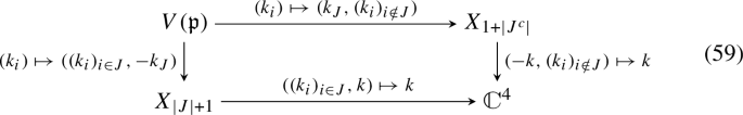
  This is for $|J|, |J^c| \ge 3$, otherwise see Remark 21. Both factors restrict the distinguished momentum $k = ({\begin{matrix} a &{} b \\ c &{} d \end{matrix}})$ to the cone ${V}(ad-bc) \subseteq {{\mathbbm {C}^{4}}}$.

• To obtain the fusion $\otimes _{{{\mathfrak {p}}},J}$ of two input sections, do in turn:⁷⁴

  • Pull them back along the projections $X_{|J|+1} \leftarrow {V}({{\mathfrak {p}}}) \rightarrow X_{1+|J^c|}$.

  • Take the tensor product.

  • Reorder the factors ${{\,\mathrm{im}\,}}S^{2h} k^\pm _i \otimes {{\mathfrak {u}}}$.

  • Annihilate the two superfluous ${{\,\mathrm{im}\,}}S^{2h} k^\pm \otimes {{\mathfrak {u}}}$ associated to the distinguished momentum k in (59), one from each input. The two ${{\,\mathrm{im}\,}}S^{2h} k^\pm$ are annihilated using (43); on each standard open in Remark 16 cancel

    $$\begin{aligned} v^{\otimes 2h} \otimes w^{\otimes 2h} \mapsto 1 \end{aligned}$$

    (60)

    The two ${{\mathfrak {u}}}$ are annihilated using ${{\mathfrak {u}}}\otimes {{\mathfrak {u}}}\rightarrow \mathbbm {C}$.

Remark 21

(Special rules). If $|J| = 2$ replace the lower left factor in (59) by one of $X^\pm$, if $|J^c| = 2$ replace the upper right factor by one of $X^\pm$. Which of $X^\pm$ is determined by requiring that the result be in ${V}({{\mathfrak {p}}})$. So if $J = \{1,2\}$:

• For ${{\mathfrak {p}}}= {{\mathfrak {p}}}_{++++}$ use $X^+ \times _{{{\mathbbm {C}^{4}}}} X^+$.

• For ${{\mathfrak {p}}}= {{\mathfrak {p}}}_{++--}$ use $X^+ \times _{{{\mathbbm {C}^{4}}}} X^-$.

• For $N\ge 5$ and ${{\mathfrak {p}}}= {{\mathfrak {p}}}_{12}^+$ use $X^+ \times _{{{\mathbbm {C}^{4}}}} X$.

All other cases are analogous.

Definition 19

(Factorization condition). For $h=1,2$ let $(B^{\sigma })$ be a collection indexed by all tuples $\sigma$ with $\ge 3$ elements: $\sigma \in \{-,+\}^{N_\sigma }$ with $N_\sigma \ge 3$. The $B^\sigma$ must be of the following type: $B^{\sigma } = B^{+,\sigma }\oplus B^{-,\sigma }$ if $N_\sigma =3$, and

$$\begin{aligned} B^{\pm ,\sigma }&\in \smash {\widetilde{{\mathcal {M}}^{\pm ,\sigma }_h}}(X^{\pm }-Z_3)&\text {if }N_\sigma =3\\ B^{\sigma }&\in (\smash {\widetilde{{\mathcal {M}}^\sigma _h}} \otimes {\mathcal {O}}_X(D))(X-Z)&\text {if }N_\sigma \ge 4 \end{aligned}$$

Then the collection $(B^\sigma )$ satisfies the factorization condition if and only if:

• If $N_\sigma = 3$ then only $B^{+,\sigma }$ with $\sigma$ any permutation of ${+}{+}{-}$, and $B^{-,\sigma }$ with $\sigma$ any permutation of ${-}{-}{+}$ are nonzero. They are up to normalization the elements in Lemma 23 times the given element in ${{\mathfrak {u}}}^{\otimes 3}$ in (53). Furthermore

  $$\begin{aligned} B^{+,+-+}\ne 0 \qquad B^{-,-+-}\ne 0 \end{aligned}$$

  (61)

• If $N_\sigma \ge 4$ then $B^{\sigma }$ is homogeneous of degree $2h + 2(N_\sigma -3)$ lower than the generators of ${\mathcal {M}}^\sigma _h$. Furthermore, for all prime divisors ${{\mathfrak {p}}}\in {\mathfrak {P}}$^75,76:

  $$\begin{aligned} {{\,\mathrm{Res}\,}}_{{\mathfrak {p}}}B^\sigma = \sum _{\begin{array}{c} J:\;{{\mathfrak {p}}}\supseteq ({Q}_J)\\ N_\sigma \notin J \end{array}} \sum _{\zeta = \pm } \Big (B^{(\sigma _J,\zeta )} \otimes _{{{\mathfrak {p}}},J} B^{(-\zeta ,\sigma _{J^c})}\Big ) \otimes {{\,\mathrm{Res}\,}}_{{\mathfrak {p}}}\frac{1}{{Q}_J} \end{aligned}$$

  (62)

  If $|J|=2$ or $|J^c|=2$ one must observe the special rules in Remark 21.

• For all $N\ge 3$, the subcollection $(B^\sigma )_{N_\sigma =N}$ is $S_N$ permutation invariant.

Remark 22

(Normalization). If $(B^\sigma )$ satisfies the factorization condition then so does $(\lambda ^{N_\sigma -2}\mu ^{N_{\sigma }^{+}-N_{\sigma }^{-}}B^\sigma )$ for all $\lambda ,\mu \in \mathbbm {C}^\times$, where $N_{\sigma }^{\pm }$ is the number of plus and minus signs in $\sigma$. Up to such transformations, any two collections $(B^\sigma )$ satisfying the factorization condition have identical $(B^{\sigma })_{N_{\sigma }=3}$.

Remark 23

(Degree of homogeneity). Using the grading on M in Definition 13, amplitudes have degree $d_N = 4+(N-1)(2h-2)$. This is compatible with (62), because fusion cancels (60) and is homogeneous of degree $-2h$, and $d_N = d_{|J|+1} + d_{1+|J^c|}-2h-2$. Incidentally, the last equation has a unique solution for every $d_3$, and $d_3=4h$ is the lowest allowed by Lemma 23.

Theorem 13

(Recursive characterization; uniqueness). Fix $h=1,2$ and ${{\mathfrak {u}}}$ as in (53). Then any two collections $(B^\sigma )$ satisfying the factorization condition are equal, up to normalization as in Remark 22.

Proof

Let $\delta B^\sigma$ be the discrepancy. It vanishes for $N_\sigma = 3$, and by induction for $N_\sigma \ge 4$. In fact, by the induction hypothesis, and since the common kernel of all ${{\,\mathrm{Res}\,}}_{{\mathfrak {p}}}$ are regular elements, we have $\delta B^\sigma \in \smash {\widetilde{{\mathcal {M}}}}(X-Z)$. Since Z has codimension $\ge 2$, Theorem 10 implies $\delta B^\sigma \in {\mathcal {M}}$. But $\delta B^\sigma$ is homogeneous of degree lower than the generators of ${\mathcal {M}}$, hence zero. $\quad \square$

Example 6

We spell out the residue factorization (62) in the special case $\sigma = {-}{+}{+}{+}$, keeping in mind the table in Theorem 9, and Remark 21:

• If ${{\mathfrak {p}}}= {{\mathfrak {p}}}_{++--}$ (analogously for ${{\mathfrak {p}}}_{+-+-}$ and ${{\mathfrak {p}}}_{+--+}$) we get

  $$\begin{aligned} {{\,\mathrm{Res}\,}}_{{{\mathfrak {p}}}} B^{-+++} \;=\; \textstyle \sum _{\zeta = \pm } (B^{+,-+\zeta } \otimes _{{{\mathfrak {p}}},12} B^{-,(-\zeta )++}) \otimes {{\,\mathrm{Res}\,}}_{{{\mathfrak {p}}}} \tfrac{1}{{Q}_{12}} \end{aligned}$$

  Both summands vanish since $B^{-,\pm ++} = 0$.

• If ${{\mathfrak {p}}}= {{\mathfrak {p}}}_{--++}$ (analogously for ${{\mathfrak {p}}}_{-+-+}$ and ${{\mathfrak {p}}}_{-++-}$) we get

  $$\begin{aligned} {{\,\mathrm{Res}\,}}_{{{\mathfrak {p}}}} B^{-+++} \;=\; \textstyle \sum _{\zeta = \pm } (B^{-,-+\zeta } \otimes _{{{\mathfrak {p}}},12} B^{+,(-\zeta )++}) \otimes {{\,\mathrm{Res}\,}}_{{{\mathfrak {p}}}} \tfrac{1}{{Q}_{12}} \end{aligned}$$

  Both summands vanish since $B^{-,-++}=0$ and $B^{+,+++}=0$.

• If ${{\mathfrak {p}}}= {{\mathfrak {p}}}_{----}$ we get

  $$\begin{aligned} {{\,\mathrm{Res}\,}}_{{\mathfrak {p}}}B^{-+++}&= \textstyle \sum _{\zeta = \pm }\; (B^{-,-+\zeta } \otimes _{{{\mathfrak {p}}},12} B^{-,(-\zeta )++}) \otimes {{\,\mathrm{Res}\,}}_{{{\mathfrak {p}}}} \tfrac{1}{{Q}_{12}} \; \\&\quad +(B^{-,-+\zeta } \otimes _{{{\mathfrak {p}}},13} B^{-,(-\zeta )++}) \otimes {{\,\mathrm{Res}\,}}_{{{\mathfrak {p}}}} \tfrac{1}{{Q}_{13}} \; \\&\quad +(B^{-,++\zeta } \otimes _{{{\mathfrak {p}}},23} B^{-,(-\zeta )-+}) \otimes {{\,\mathrm{Res}\,}}_{{{\mathfrak {p}}}} \tfrac{1}{{Q}_{23}} \end{aligned}$$

  All summands vanish since $B^{-,\pm ++} = B^{-,++\pm } = 0$.

Therefore, the residues along these seven ${{\mathfrak {p}}}$ vanish. For the final, eighth prime divisor ${{\mathfrak {p}}}= {{\mathfrak {p}}}_{++++}$ we get, dropping terms that vanish due to $B^{+,+++} = 0$:

$$\begin{aligned} \nonumber {{\,\mathrm{Res}\,}}_{{\mathfrak {p}}}B^{-+++} \;=\;\;&(B^{+,-++} \otimes _{{{\mathfrak {p}}},12} B^{+,-++}) \otimes {{\,\mathrm{Res}\,}}_{{{\mathfrak {p}}}} \tfrac{1}{{Q}_{12}}\; \nonumber \\ \nonumber&+ (B^{+,-++} \otimes _{{{\mathfrak {p}}},13} B^{+,-++}) \otimes {{\,\mathrm{Res}\,}}_{{{\mathfrak {p}}}} \tfrac{1}{{Q}_{13}}\; \nonumber \\&+ (B^{+,++-} \otimes _{{{\mathfrak {p}}},23} B^{+,+-+}) \otimes {{\,\mathrm{Res}\,}}_{{{\mathfrak {p}}}} \tfrac{1}{{Q}_{23}} \end{aligned}$$

(63)

The right hand side of (63) can be checked to vanish: either by direct calculation similar to Remark 24 below, or more easily by Proposition 11 below.

Lemma 25

(The impossibility of a single residue). For all $N \ge 4$ and all ${{\mathfrak {p}}}\in {\mathfrak {P}}$, a homogeneous element of $(\smash {\widetilde{{\mathcal {M}}}} \otimes {\mathcal {O}}_X({{\mathfrak {p}}}))(X-Z)$ of degree at least 3 lower than the generators of ${\mathcal {M}}$ is zero.

Proof

Let B be such an element. Every ${{\mathfrak {p}}}$ is minimal over some $({Q}_J)$, so ${Q}_J B \in \smash {\widetilde{{\mathcal {M}}}}(X-Z) \simeq {\mathcal {M}}$, using Theorem 10. But ${Q}_J B$ is homogeneous of degree lower than the generators of ${\mathcal {M}}$, hence zero. Hence $B=0$. $\quad \square$

Proposition 11

(Helicity violation). Every collection $(B^\sigma )$ satisfying the factorization condition has the property

• If $N_\sigma \ge 4$ then $B^\sigma = 0$ if $\sigma$ contains fewer than two $+$ or two −.

• If $N_\sigma \ge 5$ then $B^{--++\cdots +}$, known as MHV amplitudes,⁷⁷ can have nonzero residue only along the ${{\mathfrak {p}}}_{ij}^+$. The residue along ${{\mathfrak {p}}}_{12}^+$ is also zero.

Proof

By Example 6, the section $B^{-+++}$ can have residue only along ${{\mathfrak {p}}}_{++++}$, so it is zero by Lemma 25 since its degree is $2h+2$ below the generators of ${\mathcal {M}}$. This implies the first claim for $N_\sigma = 4$, for all $N_\sigma$ by induction using (62). The second claim is also by (62), here the sum over J and $\zeta$ always degenerates to at most one term. $\quad \square$

Below we show that amplitudes yield a collection $(B^\sigma )$ satisfying the factorization condition. For this collection, only $S_{N-1}\subseteq S_N$ permutation invariance is by construction. But by the next remark, this implies $S_{N}$ invariance.

Remark 24

(Permutation invariance) Suppose a collection $({B}^\sigma )$ satisfies the factorization condition, but with $S_N$ invariance of each $(B^{\sigma })_{N_\sigma =N}$ subcollection relaxed to $S_{N-1}$ invariance in the first $N-1$ factors. In particular, (62) is in force verbatim; the fact that N is always the rightmost element of $J^{c}$ is now critical. We use a vertical bar to separate the first $N-1$ factors from the last. For $N=3$, permutation invariance can only fail due to a mismatch of normalizations. For $({B}^{+,\sigma })_{N_\sigma = 3}$ define normalization constants $n_\pm \in \mathbbm {C}$ by

$$\begin{aligned} {B}^{+,++|-} = n_- B_{\text {ref}}^{++-} \qquad {B}^{+,+-|+} = n_+ B_{\text {ref}}^{+-+} \end{aligned}$$

where $B_{\text {ref}}^\sigma$ is the $S_3$ permutation invariant reference defined by Lemma 23. By (61) we have $n_+ \ne 0$. We must show $n_- = n_+$. Abbreviate

$$\begin{aligned} A&=\big (B_{\text {ref}}^{-++} \otimes _{{{\mathfrak {p}}},12} B_{\text {ref}}^{-++}\big )\otimes {{\,\mathrm{Res}\,}}_{{{\mathfrak {p}}}}\tfrac{1}{{Q}_{12}}\\ A'&=\big (B_{\text {ref}}^{-++} \otimes _{{{\mathfrak {p}}},13} B_{\text {ref}}^{-++}\big )\otimes {{\,\mathrm{Res}\,}}_{{{\mathfrak {p}}}}\tfrac{1}{{Q}_{13}}\\ A''&=\big (B_{\text {ref}}^{++-} \otimes _{{{\mathfrak {p}}},23} B_{\text {ref}}^{+-+}\big )\otimes {{\,\mathrm{Res}\,}}_{{{\mathfrak {p}}}}\tfrac{1}{{Q}_{23}} \end{aligned}$$

where ${{\mathfrak {p}}}= {{\mathfrak {p}}}_{++++}$. By (62) and Lemma 25 we have ${B}^{-++|+}=0$, hence $n_+^2 A+n_+^2 A'+n_-n_+ A''=0$ by (62). On the other hand we have $A+A'+A''=0$ by direct calculation, using the relative residues in Remark 20, the expressions in Lemma 23, the given element $U \in {{\mathfrak {u}}}^{\otimes 3}$, and:

• For YM, the Jacobi identity for the Lie algebra bracket U.

• For GR, $\epsilon _{12}\epsilon _{34} + \epsilon _{23}\epsilon _{14} + \epsilon _{31}\epsilon _{24} = 0$ and $U=1^{\otimes 3}$.

Since $n_+\ne 0$ and $A'' \ne 0$ we conclude that $n_- = n_+$. This establishes $S_3$ permutation invariance for $({B}^{+,\sigma })_{N_\sigma = 3}$, the case $({B}^{-,\sigma })_{N_\sigma = 3}$ is analogous. Now $S_{N}$ permutation invariance for $N\ge 4$ is by induction using (62).

The last theorem shows that the amplitudes in Theorem 12 satisfy the factorization condition. It entails an existence theorem for Definition 19, but beware that if existence is the only goal, there can be more direct constructions, perhaps using [34] or [5], but this is not a direction we pursue. This theorem implies, together with uniqueness in Theorem 13, that all dgLa satisfying the properties of Theorem 7 have equal amplitudes, for YM and GR respectively.

Theorem 14

(Amplitudes satisfy the factorization condition). Adopt the assumptions of Theorem 12. Then the collection $(B^\sigma )$ produced by Theorem 12, i.e. the amplitudes of YM and GR, satisfies the factorization condition.

Proof

By Remark 24 it suffices to show that $(B^\sigma )$ satisfies the factorization condition with only $S_{N-1}$ permutation invariance. The $(B^{\sigma })_{N_\sigma =3}$ are nonzero, Lorentz invariant, and homogeneous of the right degree⁷⁸ by Theorem 7. Hence they satisfy (61) and are up to normalization the elements in Lemma 23, as required. In this proof we transition freely between $B^\sigma$ and the corresponding $b^\sigma$ that use ${\mathcal {C}}$ via (52), as in the proof of Theorem 12. The $b^\sigma$ have the property (57). Let $N\ge 4$. We must show that the $B^\sigma$ have degree $2h+2(N-3)$ lower than the generators of ${\mathcal {M}}$. Equivalently, that they have degree zero using the shift ${\mathcal {M}}[4+(N-1)(2h-2)]$. This is seen as follows follows:

• Use ${\varGamma ^{}_{}}$ as a shorthand for the R-modules ${\varGamma ^{}_{i,\pm \sigma _ih}}$ that appear in (51). Endow them with an R-grading by ${\varGamma ^{}_{}}^1 \simeq R^{2h+1}$ and ${\varGamma ^{}_{}}^2 \simeq R^{4h}$ and ${\varGamma ^{}_{}}^3 \simeq R^{2h-1}$, meaning they are generated in degree zero.

• The homogeneity in Theorem 7 means that $b^\sigma$ has R-degree zero if in Eq. (51) one uses the shifts ${{\,\mathrm{Hom}\,}}({\varGamma ^{}_{}}^1[2] \otimes \cdots \otimes {\varGamma ^{}_{}}^1[2],{\varGamma ^{}_{}}^2[3])$.

• The two isomorphisms in (44) have degree zero using the shifts $({{\,\mathrm{im}\,}}S^{2h} k)[j]$ and ${\varGamma ^{}_{}}^1[j]$ and ${\varGamma ^{}_{}}^2[j-1]$. This holds for all j.⁷⁹

• The isomorphism (43) is induced by a degree zero map $({{\,\mathrm{im}\,}}S^{2h}k^\pm )[2h-2] \rightarrow (({{\,\mathrm{im}\,}}S^{2h} k^\mp )[2])^*$, with $*$ the dual.

We must show (62). To see that the residue along ${{\mathfrak {p}}}$ satisfies (62) at a given maximal ${{\mathfrak {m}}}\supseteq {{\mathfrak {p}}}$, corresponding to a point in $V({{\mathfrak {p}}})-Z$, choose homotopy data as in (57). Recall that for every internal $J\subseteq \{1,\dots ,N-1\}$ with ${{\mathfrak {p}}}\subseteq ({Q}_J)$ this involves an optimal homotopy

$$\begin{aligned} {H}_J = h + \frac{1}{{Q}_J} i {h}_{{Q}}p \end{aligned}$$

where $h,i,{h}_{{Q}}, p$ are matrices with entries in $R_{{\mathfrak {m}}}$ that depend only on $k_J$. To compute the residue along ${{\mathfrak {p}}}$ one uses:

• Tree combinatorics. There is at most one $1/{Q}_J$ in any given tree. The sum over all trees containing J as an internal line is a double sum over all trees below and all trees above J. The internal line J is decorated by ${H}_J$.

• The structure of ${H}_J$. Upon evaluation of ${{\,\mathrm{Res}\,}}_{{\mathfrak {p}}}$, the optimal homotopy inserts the matrix $i {h}_{{Q}}p$ at the internal line J. While this matrix depends on the choice of the optimal homotopy, the induced map on homology is canonical, namely the inverse of (39)⁸⁰ by Remark 10.

One obtains (62) by construction of the isomorphism (52). The sum over $\zeta = \pm$ in (62) corresponds to the direct sum of two complexes in (34). The $S_{N-1}$ permutation invariance in the first $N-1$ factors is by construction. $\quad \square$

It would be interesting to study qualitative properties of the amplitudes near Z in codimension $\ge 2$. Perhaps local cohomology calculations yield interesting constraints only based on the structure of the sheaves. The case where one $k_i$ approaches zero is known as the soft gluon respectively graviton limit.

Appendices

On the Module to Sheaf Functor

In this appendix, R is the coordinate ring of an irreducible affine $\mathbbm {C}$-variety X; hence R is a reduced affine $\mathbbm {C}$-algebra, Noetherian, and an integral domain. For every nonzero $f \in R$, the localization $R_f$ inherits these properties and it is the coordinate ring of the irreducible subvariety $D_f = \{x \in X \mid f(x) \ne 0\}$. Every localization of R is a subring of ${{\,\mathrm{Frac}\,}}(R)$.

Lemma 26

For every finitely generated R-module M there exists a unique ${\mathcal {O}}_X$-sheaf $\smash {\widetilde{M}}$ with $\smash {\widetilde{M}}(D_f) = M_f$ for all nonzero $f\in R$, and canonical restriction maps. Also $\smash {\widetilde{R}} = {\mathcal {O}}_X$, and   $\smash {\widetilde{}}$  is an exact functor from finitely generated modules to coherent sheaves, and

We also have $\smash {\widetilde{M}}|_{D_f} = \smash {\widetilde{M_f}}$.

This is in [35, Section I.1.3] or [29, Section II.5]. The second half of Lemma 26 can alternatively be taken to define the tensor product, the , and via exactness the kernel and cokernel and image of a morphism, for such sheaves. These operations are local in the sense that they commute with restriction to $D_f$, say $(M \otimes _R N)_f = M_f \otimes _{R_f} N_f$ implies

$$\begin{aligned} (\smash {\widetilde{M}} \otimes _{{\mathcal {O}}_X} \smash {\widetilde{N}})|_{D_f} = \smash {\widetilde{M}}|_{D_f} \otimes _{{\mathcal {O}}_{D_f}} \smash {\widetilde{N}}|_{D_f} \end{aligned}$$

A sheaf $\smash {\widetilde{M}}$ is locally free of rank one if every point has an open neighborhood $D_f$ such that $\smash {\widetilde{M}}|_{D_f} \simeq {\mathcal {O}}_X|_{D_f}$, that is $M_f \simeq R_f$. Local freeness on an open subset is preserved by and by the tensor product of sheaves. It is not preserved by cokernels, cf. skyscraper sheaf.

Irreducibility of a Fiber Product

The goal of this appendix is Lemma 29. Its proof does not logically require Lemmas 27 and 28 , but they are included because they convey a more geometric picture.

Lemma 27

Suppose X, Y are irreducible affine $\mathbbm {C}$-varieties, and

$$\begin{aligned} X \xrightarrow {\;\;f\;\;} {{\mathbbm {C}^{m}}} \xleftarrow {\;\;g\;\;} Y \end{aligned}$$

are morphisms of varieties. Suppose Y is Cohen–Macaulay, g is surjective, every fiber of g has dimension $\dim Y - m$, and there is an open dense subset $U \subseteq X$ such that the fiber $g^{-1}(f(x)) \subseteq Y$ is irreducible for all $x \in U$. Then

$$\begin{aligned} X \times _{{\mathbbm {C}^{m}}} Y = \{(x,y) \in X \times Y \mid f(x) = g(y) \} \end{aligned}$$

is an irreducible variety.

Proof

The morphism g is flat since Y is Cohen–Macaulay, ${{\mathbbm {C}^{m}}}$ is smooth, and the fibers of g have dimension $\dim Y - m$, see [29, Exercise III.10.9]. This is sometimes referred to as ‘miracle flatness’. The morphism g is locally of finite presentation, because the coordinate ring of Y admits a finite presentation as (via g) a $\mathbbm {C}[z_1,\ldots ,z_m]$-algebra. Flat and locally of finite presentation implies that every base change of g is open, by [35, IV.2, 2.4.6]. So base change by f yields an open map $X \leftarrow X \times _{{\mathbbm {C}^{m}}} Y$. By topology, if $X \leftarrow A$ is continuous and open, if X is irreducible, and if there is an open dense subset of X such that the corresponding fibers are irreducible, then A is irreducible. $\quad \square$

In the following, each $k_i$ has four components and each $v_i$ and $w_i$ has two components. We denote $k_i = (a_i,b_i,c_i,d_i)$ and ${Q}_i = a_id_i - b_ic_i$.

Lemma 28

(Irreducibility). Suppose X is an irreducible affine $\mathbbm {C}$-variety, and $f: X \rightarrow {{\mathbbm {C}^{4}}}$ a morphism of varieties. Let $n \ge 3$ be an integer and if $n=3$ then demand that f not be identically zero. Consider

$$\begin{aligned} X \xrightarrow {\;\;f\;\;} {{\mathbbm {C}^{4}}} \xleftarrow {\;\;(k_{1\ldots n}) \mapsto k_1 + \ldots + k_n\;\;} \mathrm{Cone}^n \end{aligned}$$

where $\mathrm{Cone} = {V}(ad-bc) \subseteq {{\mathbbm {C}^{4}}}$. Then the fiber product

$$\begin{aligned} X \times _{{{\mathbbm {C}^{4}}}}~ \mathrm{Cone}^n \end{aligned}$$

is irreducible. Same if the right map is ${{\mathbbm {C}^{4}}} \xleftarrow {(v_{1\ldots n},w_{1\ldots n}) \mapsto v_1w_1^T + \ldots + v_nw_n^T} {{\mathbbm {C}^{4n}}}$.

Proof

Clearly ${\text {Cone}}^n$ is irreducible, a complete intersection of dimension 3n, hence Cohen–Macaulay. The fibers of $g: (k_{1\ldots n}) \mapsto k_1 + \ldots + k_n$ have dimension⁸¹$3n-4$ because $(k_1 + \ldots + k_n - {{s}},{Q}_1,\ldots ,{Q}_n)$ is for all ${{s}}\in {{\mathbbm {C}^{4}}}$ a regular sequence in $\mathbbm {C}[k_{1\ldots n}]$ of length $n+4$, see Lemma 15. Let $A_n$ be the assertion that the fiber $g^{-1}({{s}})$ is irreducible for all ${{s}}\in {{\mathbbm {C}^{4}}}$, except ${{s}}=0$ if $n=3$. Note that $A_n$ implies Lemma 28 for that n, by Lemma 27. The claim $A_3$ follows from Lemma 30 below. We prove $A_n$, $n \ge 4$ by induction. Namely the fiber $k_1 + \ldots + k_n = {{s}}$ is equal to ${\text {Cone}}\times _{{{\mathbbm {C}^{4}}}} {\text {Cone}}^{n-1}$ for

$$\begin{aligned} {\text {Cone}}\xrightarrow {\;\; k_n \mapsto -k_n + {{s}}\;\;} {{\mathbbm {C}^{4}}} \xleftarrow {\;\;(k_{1 \ldots n-1}) \mapsto k_1 + \ldots + k_{n-1}\;\;} {\text {Cone}}^{n-1} \end{aligned}$$

(64)

and is irreducible because $A_{n-1}$ allows us to use Lemma 28 for $n-1$. $\quad \square$

Lemma 29

(Primality). Suppose ${{\mathfrak {p}}}\subseteq \mathbbm {C}[x_{1\ldots d}]$ is a prime ideal for some integer $d \ge 1$. Let $f \in \mathbbm {C}[x_{1\ldots d}]^4$ be four polynomials. Let $n \ge 3$ be an integer and if $n=3$ then demand that at least one of the four components of f not be in ${{\mathfrak {p}}}$. Then ${{\mathfrak {q}}}\subseteq \mathbbm {C}[x_{1\ldots d},k_{1\ldots n}]$ given by

$$\begin{aligned} {{\mathfrak {q}}}= ({{\mathfrak {p}}},k_1+\cdots + k_n - f, {Q}_1,\ldots ,{Q}_n) \end{aligned}$$

is a prime ideal. Same for ${{\mathfrak {q}}}= ({{\mathfrak {p}}},v_1w_1^T + \cdots + v_nw_n^T - f) \subseteq \mathbbm {C}[x_{1\ldots d},v_{1\ldots n},w_{1\ldots n}]$.

Proof

This proof is similar to the proof of Lemma 28, but Lemma 28 is not logically required. For every ${{s}}\in \mathbbm {C}^4$, define the ideal ${{\mathfrak {a}}}_{{s}}= (k_1 + \cdots + k_n - {{s}},{Q}_1,\ldots ,{Q}_n) \subseteq \mathbbm {C}[k_{1\ldots n}]$. Let $A_n$ be the assertion that ${{\mathfrak {a}}}_{{s}}$ is prime for all ${{s}}$, except ${{s}}=0$ if $n=3$. We first prove for all $n \ge 3$:

$$\begin{aligned} \textit{If } A_n \textit{ holds, then Lemma}~29 \textit{ holds for that } n. \end{aligned}$$

(65)

To prove (65), we will use the following two observations:

• (a) If $A_n$ holds then there exists an open dense $U \subseteq {V}({{\mathfrak {p}}})$ such that $x \in U$ implies that ${{\mathfrak {a}}}_{f(x)}$ is prime. For $n \ge 4$ take $U = {V}({{\mathfrak {p}}})$, for $n=3$ use the additional assumption on f.

• (b) There exist a monomial order for $k_{1\ldots n}$ and a Gröbner basis $G_{{s}}$ for ${{\mathfrak {a}}}_{{s}}$ whose elements are in $\mathbbm {C}[{{s}}][k_{1\ldots n}]$ (meaning their coefficients are polynomials in ${{s}}$) such that the coefficients of the leading monomials are independent of ${{s}}$.⁸²

We now prove the implication (65): Assuming $p_1p_2 \in {{\mathfrak {q}}}$, we must prove that $p_1 \in {{\mathfrak {q}}}$ or $p_2 \in {{\mathfrak {q}}}$. Denote evaluation at $x \in {V}({{\mathfrak {p}}})$ by $p_{1x},\;p_{2x} \in \mathbbm {C}[k_{1\ldots n}]$. If $x \in {V}({{\mathfrak {p}}})$ then $p_{1x}p_{2x} \in {{\mathfrak {a}}}_{f(x)}$. Set $U_i = \{x \in U \mid p_{ix} \in {{\mathfrak {a}}}_{f(x)}\}$. Primality of ${{\mathfrak {a}}}_{f(x)}$ for $x \in U$ implies $U_1 \cup U_2 = U$. Note that for $x \in U_i$, Gröbner reduction of $p_{ix}$ using the Gröbner basis $G_{f(x)}$ yields zero. Let $P_i \in \mathbbm {C}[x_{1\ldots d}][k_{1\ldots n}]$ be the result of Gröbner reduction of $p_i$ using $G_{f(x)}$ with x symbolic (crucially, by the properties in (b), no division by f(x) occurs during this Gröbner reduction). Clearly, $p_i-P_i \in {{\mathfrak {q}}}$. By construction, $P_i = 0$ if $x \in U_i$. Expand $P_i = \sum _M P_{iM} M$ where $P_{iM} \in \mathbbm {C}[x_{1\ldots d}]$ and M runs over the monomials in $k_{1\ldots n}$. For all $M_1$ and $M_2$, we have $P_{1M_1}P_{2M_2} = 0$ if $x \in U = U_1 \cup U_2$, and if $x \in {V}({{\mathfrak {p}}})$ by continuity. Hence $P_{1M_1}P_{2M_2} \in \sqrt{{{\mathfrak {p}}}} = {{\mathfrak {p}}}$ since ${{\mathfrak {p}}}$ is prime. Hence $P_{1M_1} \in {{\mathfrak {p}}}$ or $P_{2M_2} \in {{\mathfrak {p}}}$ since ${{\mathfrak {p}}}$ is prime. If $P_{1M} \in {{\mathfrak {p}}}$ for all M, then $P_1 \in {{\mathfrak {q}}}$ and then $p_1 \in {{\mathfrak {q}}}$ and we are done. If $P_{1M} \notin {{\mathfrak {p}}}$ for one M, then $P_{2M} \in {{\mathfrak {p}}}$ for all M, and then $P_2 \in {{\mathfrak {q}}}$ and then $p_2 \in {{\mathfrak {q}}}$. This concludes the proof of (65).

Given (65), it now suffices to prove $A_n$ for all $n \ge 3$. Assertion $A_3$ is in Lemma 30 below. The $A_n$ for $n \ge 4$ follow by induction on n, by a direct analog of (64). Namely, rearrange the definition of ${{\mathfrak {a}}}_{{s}}\subseteq \mathbbm {C}[k_{1\ldots n}] = \mathbbm {C}[k_n,k_{1\ldots n-1}]$ as follows:

$$\begin{aligned} {{\mathfrak {a}}}_{{s}}\;=\; ({Q}_n,k_1 + \ldots + k_{n-1} - (- k_n + {{s}}),{Q}_1,\ldots ,{Q}_{n-1}) \end{aligned}$$

By $A_{n-1}$ we can use Lemma 29 for $n-1$ ($\ge 3$) which implies that ${{\mathfrak {a}}}_{{{s}}}$ is prime for all ${{s}}$.

The proof is analogous in the case of the two-component vectors $v_i$ and $w_i$; one then works with the ideal ${{\mathfrak {a}}}_{{s}}= (v_1w_1^T + \ldots + v_nw_n^T - {{s}}) \subseteq \mathbbm {C}[v_{1\ldots n},w_{1\ldots n}]$ for each $s \in \mathbbm {C}^4$. To construct a Gröbner basis $G_{{s}}$, use a monomial ordering similar to the one in Lemma 15. $\quad \square$

The following lemma is used in the proof of Lemma 29. It may be thought of as a complement of Proposition 8, which deals with the case ${{s}}= 0$.

Lemma 30

If ${{s}}\in \mathbbm {C}^4 - 0$ then $(k_1 + k_2 + k_3 - {{s}}, {Q}_1,{Q}_2,{Q}_3) \subseteq \mathbbm {C}[k_{1\ldots 3}]$ is a prime ideal.

Proof

In this proof, $k_i$ and s are viewed as $2 \times 2$ matrices. So $k_i = ({\begin{matrix} a_i &{} b_i \\ c_i &{} d_i \end{matrix}})$ and ${Q}_i = \det k_i$. Eliminating $k_3$, it suffices to prove that $I_{{{s}}} = ({Q}_1,{Q}_2,\det (k_1+k_2-{{s}})) \subseteq \mathbbm {C}[k_1,k_2]$ is a prime ideal for all $s \in \mathbbm {C}^4 - 0$. It suffices to check this for one ${{s}}$ in every orbit of the automorphism group of the cone, say ${{s}}' = ({\begin{matrix} 1 &{} 0 \\ 0 &{} 1 \end{matrix}})$ and ${{s}}'' = ({\begin{matrix} 1 &{} 0 \\ 0 &{} 0 \end{matrix}})$. We first show that $I_{{s}}$ is the kernel of the following ring map $f_{{s}}$. Here $v_1,v_2,w_1,w_2$ have two components each.

$$\begin{aligned} f_{{s}}\;\;:\;\; \mathbbm {C}[k_1,k_2] \rightarrow \mathbbm {C}[v_1,v_2,w_1,w_2]/(\det (v_1w_1^T+v_2w_2^T-{{s}})),\quad k_i \mapsto v_iw_i^T \end{aligned}$$

This follows from the following Macaulay2 [30] calculation, see also Remark 12:⁸³

It follows that $\mathbbm {C}[k_1,k_2]/I_{{s}}$ is isomorphic to a subring of the target ring of $f_{{s}}$. But this target is an integral domain because the quartic $\det (v_1w_1^T+v_2w_2^T-{{s}})$ is an irreducible polynomial when ${{s}}={{s}}',{{s}}''$.⁸⁴ Therefore $\mathbbm {C}[k_1,k_2]/I_{{s}}$ is an integral domain, hence $I_{{s}}$ is prime [36]. $\quad \square$

References

Parke, S.J., Taylor, T.R.: An amplitude for n-gluon scattering. Phys. Rev. Lett. 56, 2459 (1986)
Mangano, M., Parke, S., Xu, Z.: Duality and multi-gluon scattering. Nucl. Phys. B 298(4), 653–672 (1988)
Britto, R., Cachazo, F., Feng, B., Witten, E.: Direct proof of the tree-level scattering amplitude recursion relation in Yang–Mills theory. Phys. Rev. Lett. 94(18), 181602 (2005)
Arkani-Hamed, N., Kaplan, J.: On tree amplitudes in gauge theory and gravity. J. High Energy Phys. 4, 76 (2008)
Arkani-Hamed, N., Bourjaily, J., Cachazo, F., Goncharov, A., Postnikov, A., Trnka, J.: Grassmannian Geometry of Scattering Amplitudes. Cambridge University Press, Cambridge (2016)
Elvang, H., Huang, Y.T.: Scattering Amplitudes in Gauge Theory and Gravity. Cambridge University Press, Cambridge (2015)
Kajiura, H.: Noncommutative homotopy algebras associated with open strings. Rev. Math. Phys. 19(01), 1–99 (2007)
Loday, J.L., Vallette, B.: Algebraic Operads, vol. 346. Springer, Berlin (2012)
Zeitlin, A.M.: Homotopy lie superalgebra in Yang–Mills theory. J. High Energy Phys. 9, 68 (2007)
Zeitlin, A.M.: Conformal field theory and algebraic structure of gauge theory. JHEP 1003, 056 (2010)
Costello, K.: Renormalization and Effective Field Theory, vol. 170. AMS, Providence (2011)
Reiterer, M., Trubowitz, E.: The graded Lie algebra of general relativity. arXiv:1412.5561 (2014) and arXiv:1812.11487 (2018)
Kontsevich, M.: Deformation quantization of Poisson manifolds. Lett. Math. Phys. 66, 157–216 (2003)
Huebschmann, J., Stasheff, J.: Formal solution of the master equation via HPT and deformation theory. Forum Math. 14, 847–868 (2002)
Berglund, A.: Homological perturbation theory for algebras over operads. Algebr. Geom. Topol. 14, 2511–2548 (2014)
Kontsevich M., Soibelman Y.: Homological mirror symmetry and torus fibrations. Symplectic geometry and mirror symmetry, 203 (2001)
Grothendieck A.: Local Cohomology. Lecture Notes in Math. 41 (1967)
Berends, F.A., Giele, W.T.: Recursive calculations for processes with \(n\) gluons. Nucl. Phys. B 306, 759–808 (1988)
Nützi, A., Reiterer, M.: Scattering amplitude annihilators. J. High Energy Phys. 2020, 20 (2020)
Reiterer, M.: A homotopy BV algebra for Yang–Mills and color-kinematics. arXiv:1912.03110 (2019)
Macrelli, T., Saemann, C., Wolf, M.: Scattering amplitude recursion relations in BV quantisable theories. Phys. Rev. D 100, 045017 (2019)
Arvanitakis, A.S.: The \(L_{\infty }\)-algebra of the S-matrix. J. High Energy Phys. 1907, 115 (2019)
Crainic, M.: On the perturbation lemma, and deformations. arXiv:math/0403266 (2004)
Gerstenhaber, M.: On the deformation of rings and algebras. Ann. Math. 79, 59–103 (1964)
Newman, E., Penrose, R.J.: An approach to gravitational radiation by a method of spin coefficients. J. Math. Phys. 3, 566–578 (1962)
Cheng, X.Z., Getzler, E.: Transferring homotopy commutative algebraic structures. J. Pure Appl. Algebra 212(11), 2535–2542 (2008)
Matsumura, H.: Commutative Ring Theory. Cambridge University Press, Cambridge (1989)
Hartshorne, R.: Generalized divisors on Gorenstein schemes. K-theory 8(3), 287–339 (1994)
Hartshorne, R.: Algebraic Geometry. Graduate Texts in Mathematics, vol. 52. Springer, Berlin (1977)
Grayson, D.R., Stillman, M.E.: Macaulay2, a software system for research in algebraic geometry. www.math.uiuc.edu/Macaulay2/
Bruns, W., Vetter, U.: Determinantal Rings. Lecture Notes in Mathematics 1327, Springer (1988)
Atiyah, M.F., MacDonald, I.G.: Introduction to Commutative Algebra. Addison-Wesley Publishing Company, Boston (1969)
Shafarevich, I.R.: Basic Algebraic Geometry, vol. 2. Springer, Berlin (1994)
Cachazo, F., Svrcek, P., Witten, E.: MHV vertices and tree amplitudes in gauge theory. J. High Energy Phys. 9, 6 (2004)
Grothendieck, A., Dieudonné, J.: Éléments de géométrie algébrique, EGA Publications Mathématiques de l’IHÉS
Christodoulou, D., Klainerman, S.: The Global Nonlinear Stability of the Minkowski Space. Princeton University Press, PMS-41, Princeton (1993)
Acknowledgements
We thank Thomas Willwacher for very useful comments on parts of this manuscript; Eugene Trubowitz for studying \(L_\infty \) algebras and homotopy transfer with us; and Horst Knörrer for his interest.
Funding
Open access funding provided by Bern University of Applied Sciences Open access funding provided by Bern University of Applied Sciences.
Author information
Authors and Affiliations
Corresponding author
Additional information
Communicated by C. Schweigert.
Publisher's Note
Springer Nature remains neutral with regard to jurisdictional claims in published maps and institutional affiliations.