
Abstract
This is the second of two works, in which we discuss the definition of an appropriate notion of mass for static metrics, in the case where the cosmological constant is positive and the model solutions are compact. In the first part, we have established a positive mass statement, characterising the de Sitter solution as the only static vacuum metric with zero mass. In this second part, we prove optimal area bounds for horizons of black hole type and of cosmological type, corresponding to Riemannian Penrose inequalities and to cosmological area bounds à la Boucher–Gibbons–Horowitz, respectively. Building on the related rigidity statements, we also deduce a uniqueness result for the Schwarzschild–de Sitter spacetime.
1 Introduction and Statement of the Main Results
In this paper we continue the study started in [14] about the notion of virtual mass of a static metric with positive cosmological constant. To make the exposition as much self-contained as possible, we briefly recall the basic notions and definitions.
1.1 Setting of the problem and preliminaries
In this paper we consider static vacuum metrics in presence of a positive cosmological constant. These are given by triples \((M,g_0, u)\) where \((M,g_0)\) is an n-dimensional compact Riemannian manifold, \(n \ge 3\), with nonempty smooth boundary \(\partial M\), and \(u \in {{\mathscr {C}}}^\infty (M)\) is a smooth nonnegative function obeying to the following system
where \(\mathrm{Ric}\), \(\mathrm{D}\), and \(\Delta \) represent the Ricci tensor, the Levi-Civita connection, and the Laplace–Beltrami operator of the metric \(g_0\), respectively, and \(\Lambda >0\) is a positive real number called cosmological constant. We will always assume that the boundary \(\partial M\) coincides with the zero level set of u, so that, in particular, u is strictly positive in the interior of M. For more detailed discussions on the legitimacy of these assumptions, we refer the reader to [5, 32]. In the rest of the paper the metric \(g_0\) and the function u will be referred to as static metric and static (or gravitational) potential, respectively, whereas the triple \((M,g_0, u)\) will be called a static solution. For a more complete justification of this terminology as well as for some comments about the physical nature of the problem, we refer the reader to the introduction of [14] and the references therein. Here, we only recall that, having at hand a solution \((M, g_0, u)\) to (1.1), it is possible to recover a static solution \((X, \gamma )\) to the vacuum Einstein field equations
just by setting \(X = {\mathbb {R}}\times M\) and letting \(\gamma \) be the Lorentzian metric defined on X by
To complete the setup of our problem, we now list some of the basic properties of static solutions to system (1.1), whose proof can be found in [5, Lemma 3] as well as in the indicated references.
-
Concerning the regularity of the function u, we know from [23, 58] that u is analytic. In particular, by the results in [54], we have that its critical level sets are discrete.
-
Since the manifold M is compact, \(\partial M = \{ u=0\}\) and \(u>0\) in \(M {\setminus } \partial M\), the static potential u achieves its maximum in the interior of M. To fix the notation, we set
$$\begin{aligned} u_{\mathrm{max}}\,\, = \,\, \max _M u \qquad \hbox {and} \qquad \mathrm{MAX}(u)=\{p\in M \, : \, u(p)=u_{\mathrm{max}}\} . \end{aligned}$$Since u is analytic, one has that, according to [44] (see also [40, Theorem 6.3.3]), the locus \(\mathrm{MAX}(u)\) is a (possibly disconnected) stratified analytic subvariety whose strata have dimensions between 0 and \(n-1\). More precisely, it holds
$$\begin{aligned} \mathrm{MAX}(u)\,=\,\Sigma ^0\sqcup \Sigma ^1\sqcup \dots \sqcup \Sigma ^{n-1}, \end{aligned}$$where \(\Sigma ^i\) is a finite union of i-dimensional analytic submanifolds, for every \(i=0,\dots ,n-1\). This means that, given a point \(p\in \Sigma ^i\), there exists a neighborhood \(p\in \Omega \subset M\) and an analytic diffeomorphism \(f:\Omega \rightarrow {\mathbb {R}}^n\) such that
$$\begin{aligned} f(\Omega \cap \Sigma ^i)\,=\,L\cap f(\Omega ), \end{aligned}$$for some i-dimensional linear space \(L\subset {\mathbb {R}}^n\). In particular, the set \(\Sigma ^{n-1}\) is a smooth analytic hypersurface and it will play an important role in what follows. We will refer to the hypersurface \(\Sigma ^{n-1}\) as the top stratum of \(\mathrm{MAX}(u)\).
-
Taking the trace of the first equation in (1.1) and substituting the result into the second one, it is immediate to deduce that the scalar curvature of the metric \(g_0\) is constant, and more precisely it holds
$$\begin{aligned} {\mathrm R}=2\Lambda . \end{aligned}$$(1.3)In particular, we observe that choosing a normalization for the cosmological constant corresponds to fixing a scale for the metric \(g_0\). Throughout the paper we will choose the following normalization
$$\begin{aligned} \Lambda \, = \, \frac{n(n-1)}{2} . \end{aligned}$$(1.4)So that in particular the manifold \((M, g_0)\) will have constant scalar curvature \({\mathrm R}\equiv n(n-1)\).
-
The boundary \(\partial M = \{u=0\}\), which is assumed to be a smooth submanifold of M, is also a regular level set of u. In particular it follows from the equations that it is a (possibly disconnected) totally geodesic hypersurface in \((M,g_0)\). The connected components of \(\partial M\) will be referred to as horizons. In Definition 2 below, we will distinguish between horizons of black hole type, horizons of cosmological type and horizon of cylindrical type. In order to simplify the exposition of some of the results in the paper, it is convenient to suppose that the manifold M is orientable. This of course is not restrictive. In fact, if the manifold is not orientable, we can consider its orientable double covering, and transfer the results obtained on this latter to the original manifold by means of the projection. We recall that an orientation of M induces an orientation on the boundary \(\partial M\), therefore, in particular, if M is orientable so are the horizons.
-
Finally, one has that the quantity \(|\mathrm{D}u|\) is locally constant and positive on \(\partial M\). Notice that the value of \(|\mathrm{D}u|\) at a horizon depends on the choice of the normalization of u. A more invariant quantity is the so called surface gravity of an horizon S, which can be defined as the constant
$$\begin{aligned} \kappa (S)\,\,=\,\,\frac{|\mathrm{D}u|_{|_S}}{u_{\mathrm{max}}} , \end{aligned}$$(1.5)where we recall that \(u_{\mathrm{max}}\) is the maximum of u in M. For a more precise explaination of the physical motivations behind this definition, we refer the reader to [14].
Recasting all the normalizations that we have introduced so far, we are led to study the following system
This system is of course equivalent to (1.1), with some of the assumptions made more explicit. In this work, we are interested in the classification of static triples up to isometry, or at least up to a finite covering. Even though these notions are quite natural, we recall their precise definitions in the setting of static triples.
Definition 1
We say that two triples \((M,g_0,u)\) and \((M',g_0',u')\) are isometric if there exists a Riemannian isometry \(F:(M,g_0)\rightarrow (M',g_0')\) such that, up to a normalization of u, it holds \(u=u'\circ F\). We say that \((M,g_0,u)\) is a covering of \((M',g_0',u')\) if there exists a Riemannian covering \(F:(M,g_0)\rightarrow (M',g_0')\) such that, up to a normalization of u, it holds \(u=u'\circ F\).
It is worth remarking that, for the most part, the results in this paper allow for a classification up to isometry of the solutions. However, as we will discuss more precisely in Remark 1, there is one example of a static triple that is not simply connected. In order to include this special case in our statements, it will be occasionally necessary to argue up to covering. We conclude this subsection introducing some more terminology, whose meaning will be clarified in the next subsection by the detailed description of the rotationally symmetric solutions to (1.6).
Definition 2
Let \((M, g_0, u)\) be a solution to problem (1.6). A connected component S of \(\partial M\) is called an horizon. An horizon is said to be:
-
of cosmological type if: \(\kappa (S) \,<\, \sqrt{n}\),
-
of black hole type if: \(\kappa (S) \,>\, \sqrt{n}\),
-
of cylindrical type if: \(\kappa (S) \,=\, \sqrt{n}\)
where \(\kappa (S)\) is the surface gravity of S defined in (1.5). A connected component N of \(M {\setminus } \mathrm{MAX}(u)\) is called region and we will denote by \(\partial N\) the collection of the horizons of M that lie in N, namely
A region N is said to be:
-
an outer region if all of its horizons are of cosmological type, i.e., if
$$\begin{aligned} \max _{S \in \pi _0(\partial N)} \kappa (S) \,<\, \sqrt{n}, \end{aligned}$$ -
an inner region if it has at least one horizon of black hole type, i.e., if
$$\begin{aligned} \max _{S \in \pi _0(\partial N)} \kappa (S) \,>\, \sqrt{n}, \end{aligned}$$ -
a cylindrical region if there are no horizons of black hole type and there is at least one horizon of cylindrical type, i.e., if
$$\begin{aligned} \max _{S \in \pi _0(\partial N)} \kappa (S) \,=\, \sqrt{n}. \end{aligned}$$
1.2 Rotationally symmetric solutions
In this subsection, we briefly recall the rotationally symmetric solutions to (1.6). These have three different qualitative behaviour, depending on the value of the mass parameter m, which is allowed to vary in the real interval \([0, m_{\mathrm{max}}]\), where
We observe that if the number \(m_{\mathrm{max}}\) is defined as above, then for every \(0<m<m_{\mathrm{max}}\) the equation \(f_m(r) = 0\), where \(f_m(r)=1 - r^2 - 2m\,r^{2-n}\), has exactly two positive solutions \(0< r_-(m)< r_+(m)< 1\). Moreover, in the interval \([r_-(m),r_+(m)]\) the function \(f_m(r)\) assumes its maximum value at \(r_0(m)=[(n-2)m]^{1/n}\). For \(m=0\), one has that \(r_0(0)=r_-(0)=0\) and \(r_+(0)=1\), whereas for \(m=m_{\mathrm{max}}\), one has \(r_0(m_{\mathrm{max}})=r_-(m_{\mathrm{max}}) = r_+(m_{\mathrm{max}}) = [(n-2)/n]^{1/2}\).
-
de Sitter solution [27] (\(m=0\)), Fig. 1a.
$$\begin{aligned}&M \, = \, \overline{B(0,1)}\subset {\mathbb {R}}^n , \qquad g_0 \, = \, \frac{d|x|\otimes d|x|}{1-|x|^2}+|x|^2 g_{{\mathbb {S}}^{n-1}} , \nonumber \\&u \, = \, \sqrt{1-|x|^2} . \end{aligned}$$(1.8)It is not hard to check that both the metric \(g_0\) and the function u, which a priori are well defined only in the interior of \(M{\setminus } \{ 0\}\), extend smoothly up to the boundary and through the origin. This model solution can be seen as the limit of the following Schwarzschild–de Sitter solutions (1.9), when the parameter \(m \rightarrow 0^+\). The de Sitter solution is such that the maximum of the potential is \(u_{\mathrm{max}}=1\), and it is achieved at the origin. Moreover, this solution has only one connected horizon with surface gravity
$$\begin{aligned} |\mathrm{D}u| \,\, \equiv \,\, 1 \qquad \hbox {on} \quad \partial M . \end{aligned}$$Hence, according to Definition 2 below, this horizon is of cosmological type.
-
Schwarzschild–de Sitter solutions [38] (\(0<m< m_{\mathrm{max}}\)), Fig. 1b.
$$\begin{aligned}&M \, = \, \overline{B(0,r_+(m))} {\setminus } B(0, r_-(m)) \subset {\mathbb {R}}^n , \nonumber \\&g_0 \, = \, \frac{d|x|\otimes d|x|}{1-|x|^2- 2m |x|^{2-n}}+|x|^2 g_{{\mathbb {S}}^{n-1}} , \nonumber \\&u \, = \, \sqrt{1-|x|^2- 2m |x|^{2-n}}. \end{aligned}$$(1.9)Fig. 1 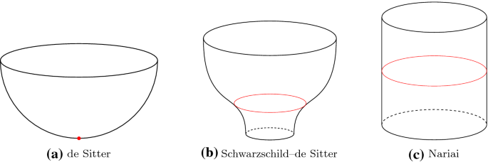
Rotationally symmetric solutions to problem (1.6). The red dot and red lines represent the set \(\mathrm{MAX}(u)\) for the three models
Here \(r_-(m)\) and \(r_+(m)\) are the two positive solutions to \(1-r^2-2mr^{2-n}=0\). We notice that, for \(r_-(m),r_+(m)\) to be real and positive, one needs (1.7). It is not hard to check that both the metric \(g_0\) and the function u, which a priori are well defined only in the interior of M, extend smoothly up to the boundary. This latter has two connected components with different character
$$\begin{aligned} \partial M_+ = \,\, \{ |x| = r_+(m)\} \qquad \hbox {and} \qquad \partial M_- = \,\, \{ |x| = r_-(m)\} . \end{aligned}$$In fact, it is easy to check (see formulæ (1.12) and (1.13)) that the normalized surface gravities satisfy
$$\begin{aligned} \kappa (\partial M_+)\,\,=\,\,\frac{|\mathrm{D}u |_{|_{\partial M_+}}}{u_{\mathrm{max}}} \,\, < \,\, \sqrt{n} \qquad \hbox {and} \qquad \kappa (\partial M_-)\,\,=\,\,\frac{|\mathrm{D}u |_{|_{\partial M_-}}}{u_{\mathrm{max}}} \,\, > \,\, \sqrt{n} . \end{aligned}$$Hence, according to Definition 2 below, one has that \(\partial M_+\) is of cosmological type, whereas \(\partial M_-\) is of black hole type. Furthermore, it holds
$$\begin{aligned} u_{\mathrm{max}}\,=\,\sqrt{1-\left( \frac{m}{m_{\mathrm{max}}}\right) ^{{2}/{n}}},\qquad \mathrm{MAX}(u)\,=\,\left\{ |x|=r_0(m)\right\} , \end{aligned}$$(1.10)where we recall that \(r_0(m)=[(n-2)m]^{1/n}\). Notice that \(M {\setminus } \mathrm{MAX} (u)\) has exactly two connected components: \(M_+\) with boundary \(\partial M_+\) and \(M_-\) with boundary \(\partial M_-\). According to Definition 2, we have that \(M_+\) is an outer region, whereas \(M_-\) is an inner region.
-
Nariai solution [46] (\(m=m_{\mathrm{max}}\)), Fig. 1c.
$$\begin{aligned}&M \, = \, [0,\pi ]\times {\mathbb {S}}^{n-1}, \qquad g_0 \, = \, \frac{1}{n}\,\big [d r\otimes d r+(n-2)\,g_{{\mathbb {S}}^{n-1}}\big ], \nonumber \\&u \, = \, \sin (r) . \end{aligned}$$(1.11)This model solution can be seen as the limit of the previous Schwarzschild–de Sitter solutions, when the parameter \(m \rightarrow m_{\mathrm{max}}^-\), after an appropriate rescaling of the coordinates and potential u (this was shown for \(n=3\) in [31] and then generalized to all dimensions \(n\ge 3\) in [21], see also [17, 18]). In this case, we have \(u_{\mathrm{max}}=1\) and \(\mathrm{MAX}(u)=\{\pi /2\}\times {\mathbb {S}}^{n-1}\). Moreover, the boundary of M has two connected components with the same constant value of the surface gravity, namely
$$\begin{aligned} |\mathrm{D}u| \,\, \equiv \,\, \sqrt{n} \qquad \hbox {on} \quad \partial M . \end{aligned}$$

In Sect. 1.3, we are going to use the above listed solutions as reference configurations in order to define the concept of virtual mass of a solution \((M, g_0, u)\) to (1.6). To this aim, it is useful to introduce the functions \(k_+\) and \(k_-\), whose graphs are plotted, for \(n=3\), in Fig. 2. They represent the normalized surface gravities of the model solutions as functions of the mass parameter m.
-
The outer surface gravity function
$$\begin{aligned} k_+ : [\, 0, m_{\mathrm{max}}) \longrightarrow [\, 1, \sqrt{n} \, ) \end{aligned}$$(1.12)is defined by
$$\begin{aligned} k_+(0) \,&= \, 1 ,\quad \qquad \qquad \qquad \qquad \qquad \qquad \;\;\qquad \qquad \hbox {for} \quad m=0, \\ k_+(m) \,&=\, \sqrt{\frac{r_+^2(m)\left[ 1-\big (r_0(m)/r_+(m)\big )^n\right] ^2}{1-\left( m / {m_{\mathrm{max}}}\right) ^{2/n}}},\quad \hbox {if} \quad 0<m<m_{\mathrm{max}}, \end{aligned}$$where \(r_+(m)\) is the largest positive root of the polynomial \(P_m(r) = r^{n-2}-r^n-2m\). Loosely speaking, \(k_+(m)\) is nothing but the constant value of \(|\mathrm{D}u|/u_{\mathrm{max}}\) at \(\{ |x| = r_+(m) \}\) for the Schwarzschild–de Sitter solution with mass parameter equal to m. We also observe that \(k_+\) is continuous, strictly increasing and \(k_+(m) \rightarrow \sqrt{n}\), as \(m \rightarrow m_{\mathrm{max}}^-\).
-
The inner surface gravity function
$$\begin{aligned} k_- : ( 0, m_{\mathrm{max}}\,] \longrightarrow [\, \sqrt{n}, +\infty \, ) \end{aligned}$$(1.13)is defined by
$$\begin{aligned} k_-(m_{\mathrm{max}}) \,&= \, \sqrt{n} , \qquad \qquad \qquad \qquad \qquad \qquad \qquad \qquad \quad \hbox {for} \quad m=m_{\mathrm{max}}, \\ k_-(m) \,&=\, \sqrt{\frac{r_-^2(m)\left[ 1-\big (r_0(m)/r_-(m)\big )^n\right] ^2}{1-\left( m / {m_{\mathrm{max}}}\right) ^{2/n}}}, \quad \hbox {if} \quad 0<m<m_{\mathrm{max}}, \end{aligned}$$where \(r_{-}(m)\) is the smallest positive root of the polynomial \(P_m(r) = r^{n-2}-r^n-2m\). Loosely speaking, \(k_-(m)\) is nothing but the constant value of \(|\mathrm{D}u|/u_{\mathrm{max}}\) at \(\{ |x| = r_-(m) \}\) for the Schwarzschild–de Sitter solution with mass parameter equal to m. We also observe that \(k_-\) is continuous, strictly decreasing and \(k_-(m) \rightarrow + \infty \), as \(m \rightarrow 0^+\).

Plot of the surface gravities \(|\mathrm{D}u|/u_{\mathrm{max}}\) of the two boundaries of the Schwarzschild–de Sitter solution (1.9) as a function of the mass m for \(n=3\). The red line represents the surface gravity of the boundary \(\partial M_+ = \{r = r_+(m)\}\), whereas the blue line represents the surface gravity of the boundary \(\partial M_- = \{r = r_-(m)\}\). Notice that for \(m=0\) we recover the constant value \(|\mathrm{D}u| \equiv 1\) of the surface gravity on the (connected) cosmological horizon of the de Sitter solution (1.8). The other special situation is when \(m=m_{\mathrm{max}}\). In this case the plot assigns to \(m_{\mathrm{max}}= 1/(3 \sqrt{3})\) the unique value \(\sqrt{3}\) achieved by the surface gravity on both the connected components of the boundary of the Nariai solution (1.11)
This concludes the list of rotationally symmetric solutions. However, it is worth mentioning that in higher dimensions there is a simple generalization of the above model triples. In fact, one can replace the spherical fibers in the Schwarzschild–de Sitter solution (1.9) with any \((n-1)\)-dimensional Einstein manifold \((E^{n-1},g_{E^{n-1}})\) with \(\mathrm{Ric}_{E^{n-1}}=(n-2)g_{E^{n-1}}\). The resulting triple is still a solution to (1.6), and it will be called generalized Schwarzschild–de Sitter solution
Analogously, one can define the generalized Nariai solution as the triple
where, again, \((E^{n-1},g_{E^{n-1}})\) is an \((n-1)\)-dimensional Einstein manifold with \(\mathrm{Ric}_{E^{n-1}}=(n-2)g_{E^{n-1}}\). Of course, the generalized solutions (1.14) and (1.15) are relevant only for \(n\ge 5\), since for \(n=3,4\) the only \((n-1)\)-dimensional Einstein manifold with \(\mathrm{Ric}_{E^{n-1}}=(n-2)g_{E^{n-1}}\) is the round sphere \(({\mathbb {S}}^{n-1},g_{{\mathbb {S}}^{n-1}})\). We also mention that, exploiting a previous work of Bohm about the existence of ’non round’ Einstein metrics on spheres [12], Gibbons, Hartnoll and Pope in [29] were able to exhibit infinite families of solutions to problem (1.6), in dimension \(4\le n\le 8\). These solutions are such that their boundary is connected and diffeomorphic to a \((n-1)\)-dimensional sphere. However, they do not have a warped product structure. This suggests that a complete classification of the solutions to problem (1.6) in dimension \(n\ge 4\) is a very hard task. On the other hand, in dimension \(n=3\), the only known solutions are the de Sitter, Schwarzschild–de Sitter and Nariai triple. The question of whether these are the only ones is still open, although there are some partial results. For instance, in [37, 41] it is proven that these models are the only locally conformally flat static metrics, in [47] this result has been extended to the Bach-flat case and in [26] the case of cyclic parallel Ricci tensor has been discussed. Some pinching conditions implying the same classification are provided in [5, 9]. Moreover, some further characterizations of the de Sitter metric have been proven in [16, 22, 32].
Since it will be of some importance in the forthcoming discussion, we conclude this section recalling the definition of Schwarzschild metric with mass parameter equal to \(m>0\). This is the simplest (and also the early) example of a non flat static metric in the case where the cosmological constant in the Einstein Field Equations (1.2) is taken to be zero.
-
Schwarzschild solutions [51] (\(m>0\)).
$$\begin{aligned}&M \, = \, {\mathbb {R}}^n {\setminus } {B(0,r_s(m))} \subset {\mathbb {R}}^n , \qquad g_0 \, = \, \frac{d|x|\otimes d|x|}{1- 2m |x|^{2-n}}+|x|^2 g_{{\mathbb {S}}^{n-1}} , \nonumber \\&u \, = \, \sqrt{1- 2m |x|^{2-n}} . \end{aligned}$$(1.16)Here, the so called Schwarzschild radius \(r_s(m) = (2m)^{1/(n-2)}\) is the only positive solution to \(1-2mr^{2-n}=0\). It is not hard to check that both the metric \(g_0\) and the function u, which a priori are well defined only in the interior of M, extend smoothly up to the boundary.
1.3 The virtual mass
As already discussed in [14], in the case of a positive cosmological constant there does not seem to be a general consensus about what the right notion of mass should be. For some possible approaches, as well as for more insights on the problems posed by the case \(\Lambda >0\), we refer the reader to the following references [1, 6,7,8, 24, 36, 45, 52, 53, 56]. In our previous work [14], we have introduced a different point of view, leading to a new notion of mass, that we now recall.
Definition 3
(Virtual Mass). Let \((M, g_0, u)\) be a solution to (1.6) and let N be a connected component of \(M {\setminus } \mathrm{MAX} (u)\). The virtual mass of N is denoted by \(\mu (N, g_0,u)\) and it is defined in the following way:
-
(i)
If N is an outer region, then we set
$$\begin{aligned} \mu (N,g_0,u) \,\, = \,\, k_+^{-1} \left( \max _{\partial N} \frac{|\mathrm{D}u |}{u_{\mathrm{max}}} \right) , \end{aligned}$$(1.17)where \(k_+\) is the outer surface gravity function defined in (1.12).
-
(ii)
If N is an inner region, then we set
$$\begin{aligned} \mu (N, g_0, u) \,\, = \,\, k_-^{-1} \left( \max _{\partial N} \frac{|\mathrm{D}u |}{u_{\mathrm{max}}} \right) , \end{aligned}$$(1.18)where \(k_-\) is the inner surface gravity function defined in (1.13).
In other words, the virtual mass of a connected component N of \(M{\setminus } \mathrm{MAX} (u)\) can be thought as the mass (parameter) that on a model solution would be responsible for (the maximum value of) the surface gravity measured at \(\partial N\). In this sense the rotationally symmetric solutions described in Sect. 1.2 are playing here the role of reference configurations. As it is easy to check, if \((M, g_0, u)\) is either the de Sitter, or the Schwarzschild–de Sitter, or the Nariai solution, then the virtual mass coincides with the explicit mass parameter m that appears in Sect. 1.2.
It is important to notice that it is not a priori guaranteed that the above definition is well posed. In fact, it could happen that the boundary of a connected component is empty or that the value of the normalized surface gravity does not lie in the range of either \(k_+\) or \(k_-\). The first possibility can be easily excluded arguing as in the No Island Lemma (see [14, Lemma 5.1]), whereas to exclude the second possibility we need to invoke [14, Theorem 2.2]. This result tells us that, on any region N of a solution \((M,g_0,u)\), it holds
and the equality is fulfilled only if \((M,g_0,u)\) is isometric to the de Sitter solution (1.8). As an immediate consequence we obtain the following Positive Mass Statement for static metrics with positive cosmological constant.
Theorem 1.1
(Positive Mass Statement for Static Metrics with Positive Cosmological Constant) Let \((M,g_0,u)\) be a solution to problem (1.6). Then, every connected component of \(M{\setminus }\mathrm{MAX}(u)\) has well–defined and thus nonnegative virtual mass. Moreover, as soon as the virtual mass of some connected component vanishes, the entire solution \((M, g_0,u)\) is isometric to the de Sitter solution (1.8).
We refer the reader to [14] for a more detailed discussion about the above statement as well as for a comparison with the classical Positive Mass Theorem proved by Schoen and Yau [49, 50] (and with a different proof by Witten [55]) for the ADM-mass of asymptotically flat manifolds with nonnegative scalar curvature.
1.4 Area bounds
An important feature of the above positive mass statement is that it gives a complete characterisation of the zero mass solutions. Another very interesting and nowadays classical characterisation of the de Sitter solution is given by the Boucher–Gibbons–Horowitz area bound [16], which in our framework can be phrased as follows
Theorem 1.2
(Boucher–Gibbons–Horowitz Area Bound). Let \((M^3,g_0,u)\) be a 3-dimensional solution to problem (1.6) with connected boundary \(\partial M\). Then, the following inequality holds
Moreover, the equality is fulfilled if and only if \((M^3, g_0, u)\) is isometric to the de Sitter solution (1.8).
Having at hand Theorems 1.1 and 1.2, it is natural to ask if in the case where the virtual mass is strictly positive and the boundary of M is allowed to have several connected components, it is possible to provide a refined version of both statements, whose rigidity case characterises now the Schwarzschild–de Sitter solutions described in (1.9) instead of the de Sitter solution. In accomplishing this program, we are inspired by the well known relation between the Positive Mass Theorem and the Riemannian Penrose Inequality as they are stated in the classical setting, where \(M^3\) is an asymptotically flat Riemannian manifold with nonnegative scalar curvature. To be more concrete, we report a simplified version of these statements in the case where the 3-manifold has one end and at most one compact horizon.
Theorem 1.3
Let \((M^3, g_0)\) be a 3-dimensional complete asymptotically flat Riemannian manifold with nonnegative scalar curvature and ADM-mass \(m_{ADM}(M^3,g_0)\) equal to \(m\in {\mathbb {R}}\). Then, the following statements hold.
-
(i)
Positive Mass Theorem (Schoen-Yau [49, 50], Witten [55]). The number m is always nonnegative
$$\begin{aligned} 0 \, \le \, m . \end{aligned}$$Moreover, the equality is fulfilled if and only if \((M^3, g_0, u)\) is isometric to the flat Euclidean space with \(u \equiv 1\).
-
(ii)
Riemannian Penrose Inequality (Huisken-Ilmanen [33], Bray [19]). Assume that the boundary of M is non empty and given by a connected, smooth and compact outermost minimal surface. Then, the following inequality holds
$$\begin{aligned} \sqrt{\frac{|\partial M|}{16 \pi }} \, \le \, m . \end{aligned}$$(1.20)Moreover, the equality is fulfilled if and only if \((M^3, g_0, u)\) is isometric to the Schwarzschild solution (1.8) with mass parameter equal to m.
For the precise definitions of asymptotically flat manifold and ADM-mass, we refer the reader to the above cited references. We also observe that in the original statement of the Positive Mass Theorem, the 3-manifold \((M^3, g)\) is a priori allowed to have a finite number of ends and that the rigidity statement holds in a stronger way, meaning that as soon as the mass of one end is vanishing, then the whole manifold is isometric to the Euclidean space. Concerning the Riemannian Penrose Inequality, it is worth pointing out that in the original statement by Huisken and Ilmanen [33, Main Theorem], the boundary of M is a priori allowed to have a finite number of connected component, namely \(\partial M = S_0 \, \sqcup \, S_1\, \sqcup \, \ldots \, \sqcup \,S_K \), and the authors are able to prove the following inequality
where \(m = m_{ADM}(M^3,g)\). With a different proof, Bray is able to recover in [19, Theorem 1] a stronger version of the above inequality, namely
Of course, when \(\partial M\) is connected, the two inequalities are the same and they reduce to (1.20). To introduce our first main result, we focus on this simple version of the Riemannian Penrose Inequality and we observe that, using the definition of the Schwarzschild radius given below formula (1.16), it can be rephrased as follows
where \(m = m_{ADM}(M^3,g)\). Having these considerations in mind, we can now state one of the main results of the present paper.
Theorem 1.4
(Refined Area Bounds). Let \((M^3,g_0,u)\) be a 3-dimensional solution to problem (1.6) and let N be a connected component of \(M^3{\setminus }\mathrm{MAX}(u)\) with virtual mass
Let \(S\subseteq \partial N\) be the horizon with the largest surface gravity in N, namely
Then, S is diffeomorphic to the sphere \({\mathbb {S}}^2\). Moreover, the following inequalities hold:
-
(i)
Cosmological Area Bound If N is an outer region, then
$$\begin{aligned} |S|\,\le \,4\pi r_+^{2}(m). \end{aligned}$$(1.21)Moreover, if the equality is fulfilled and \(S=\partial N\), then the triple \((M^3,g_0,u)\) is isometric to the Schwarzschild–de Sitter solution (1.9) with mass m.
-
(ii)
Riemannian Penrose Inequality If N is an inner region, then
$$\begin{aligned} |S|\,\le \,4\pi r_-^{2}(m). \end{aligned}$$(1.22)Moreover, if the equality is fulfilled and \(S=\partial N\), then the triple \((M^3,g_0,u)\) is isometric to the Schwarzschild–de Sitter solution (1.9) with mass m.
-
(iii)
Cylindrical Area Bound If N is a cylindrical region, then
$$\begin{aligned} |S|\,\le \,\frac{4\pi }{3}, \end{aligned}$$(1.23)Moreover, if the equality is fulfilled and \(S=\partial N\), then the triple \((M^3,g_0,u)\) is covered by the Nariai solution (1.11).
Remark 1
Notice that the rigidity statements are only in force when \(\partial N\) is connected. Concerning the rigidity statement in point (iii) of the above theorem, we observe that there is only one orientable triple which is not isometric to the 3-dimensional Nariai solution but that is covered by it, which is the quotient of the Nariai triple by the involution
where we have denoted by \(-x\) the antipodal point of x on \({\mathbb {S}}^2\). The existence of this solution was pointed out in [5, Section 7].
About the previous statement some comments are in order. First, the fact that S is necessarily diffeomorphic to a sphere is not a new result. In fact, a stronger result is already known from [5, Theorem B], where it is shown that every connected component of the boundary of a static solution to problem (1.6) is diffeomorphic to a sphere. Our approach allows to prove the same topological result, but only in the case where the horizons of \((M^3, g_0, u)\) are somehow separated from each other by the locus \(\mathrm{MAX}(u)\). Concerning the area bounds, we observe that, conceptually speaking, the inequality (1.21) should be compared with the Boucher–Gibbons–Horowitz Area Bound (1.19), since it involves the cosmological horizons of the solution, whereas the inequality (1.22) should be compared with (1.20) since it is a statement about horizons of black hole type.
An analogous statement holds in higher dimension, giving the natural analog of the inequality
which has been obtained by Chru\(\grave{\mathrm{s}}\)ciel in [22, Section 6] in the case of connected boundary, extending the Boucher–Gibbons–Horowitz method to every dimension \(n\ge 3\). Of course, in the above inequality \({\mathrm R}^{\partial M}\) stands for the scalar curvature of the boundary. Moreover, the equality is fulfilled if and only if \((M,g_0,u)\) coincides with the de Sitter solution.
Theorem 1.5
Let \((M,g_0,u)\) be a solution to problem (1.6) of dimension \(n\ge 3\), and let N be a connected component of \(M{\setminus }\mathrm{MAX}(u)\) with connected smooth compact boundary \(\partial N\). We then let \(m \in (0, m_{\mathrm{max}}]\) be the virtual mass of N, namely
Let \(S\subseteq \partial N\) be the horizon with the largest surface gravity in N, namely
Then, the following inequalities hold:
-
(i)
If N is an outer region, then
$$\begin{aligned} |S|\,\le \, \left( \int _{S} \frac{{\mathrm R}^{S}}{(n-1)(n-2)}\,\mathrm{d}\sigma \right) \, r_+^{2}(m). \end{aligned}$$(1.25)Moreover, if the equality is fulfilled and \(S=\partial N\), then \((M,g_0,u)\) is isometric to the Schwarzschild–de Sitter solution (1.9) with mass m, for \(n=3,4\). Whereas for \(n\ge 5\) it is isometric to some generalized Schwarzschild–de Sitter solution (1.14) with Einstein fiber.
-
(ii)
If N is an inner region, then
$$\begin{aligned} |S|\,\le \, \left( \int _{S} \frac{{\mathrm R}^{S}}{(n-1)(n-2)}\,\mathrm{d}\sigma \right) \, r_-^{2}(m). \end{aligned}$$(1.26)Moreover, if the equality is fulfilled and \(S=\partial N\), then \((M,g_0,u)\) is isometric to the Schwarzschild–de Sitter solution (1.9) with mass m, for \(n=3,4\). Whereas for \(n\ge 5\) it is isometric to some generalized Schwarzschild–de Sitter solution (1.14) with Einstein fiber.
-
(iii)
If N is a cylindrical region, then
$$\begin{aligned} |S|\,\le \, \int _{S}\frac{{\mathrm R}^{S}}{n(n-1)}\,\mathrm{d}\sigma . \end{aligned}$$(1.27)Moreover, if the equality is fulfilled and \(S=\partial N\), then \((M,g_0,u)\) is covered by the Nariai solution (1.11), for \(n=3,4\). Whereas for \(n\ge 5\) it is covered by some generalized Nariai solution (1.15) with Einstein fiber.
The proof of the above statement will be given in Sect. 5, except for the rigidity statements, whose proof will be discussed in Sect. 6, and for the cylindrical case, that will be discussed in Sect. 8. It is clear that Theorem 1.4 follows directly from Theorem 1.5, applying the Gauss-Bonnet formula. We also mention that the rigidity statement for Theorem 1.5 will be deduced by some more general statements (see Corollaries 6.1, 6.5 and 8.7) which correspond to some balancing formulas, in the case where the boundary of N is allowed to have several connected components. The inequalities proven in Theorem 1.5 share some analogies with the ones developed in [28, 57], see in particular [57, Theorem B].
Our approach will also allow us to prove some area lower bounds on the horizons. These lower bounds do not require the connectedness of the boundary of our region N and depend on the area of the hypersurface \(\Sigma _N\subseteq \mathrm{MAX}(u)\) that separates N from the rest of the manifold.
Theorem 1.6
(Area Lower Bound). Let \((M,g_0,u)\) be a solution to problem (1.6) of dimension \(n\ge 3\), and let N be a connected component of \(M{\setminus }\mathrm{MAX}(u)\) with connected smooth compact boundary \(\partial N\). We let \(m \in (0, m_{\mathrm{max}}]\) be the virtual mass of N, namely
Let \(\Sigma _N={\overline{N}}\cap \overline{M{\setminus } {\overline{N}}}\) be the possibly stratified hypersurface separating N from the rest of the manifold M. Then, the following inequalities hold:
-
(i)
If N is an outer region, then
$$\begin{aligned} |\partial N|\,\ge \, \left[ \frac{r_+(m)}{r_0(m)}\right] ^{n-1}\,|\Sigma _N|, \end{aligned}$$(1.28)and the equality is fulfilled if and only if \((M,g_0,u)\) is isometric to the Schwarzschild–de Sitter solution (1.9) with mass m, for \(n=3,4\). Whereas for \(n\ge 5\) it is isometric to some generalized Schwarzschild–de Sitter solution (1.14) with Einstein fiber.
-
(ii)
If N is an inner region, then
$$\begin{aligned} |\partial N|\,\ge \, \left[ \frac{r_-(m)}{r_0(m)}\right] ^{n-1}\,|\Sigma _N|, \end{aligned}$$(1.29)and the equality is fulfilled if and only if \((M,g_0,u)\) is isometric to the Schwarzschild–de Sitter solution (1.9) with mass m, for \(n=3,4\). Whereas for \(n\ge 5\) it is isometric to some generalized Schwarzschild–de Sitter solution (1.14) with Einstein fiber.
-
(iii)
If N is a cylindrical region, then
$$\begin{aligned} |\partial N|\,\ge \, |\Sigma _N|, \end{aligned}$$(1.30)and the equality is fulfilled if and only if \((M,g_0,u)\) is covered by the Nariai solution (1.11), for \(n=3,4\). Whereas for \(n\ge 5\) it is covered by some generalized Nariai solution (1.15) with Einstein fiber.
In the notations of Theorem 1.6, if we also assume that \(\partial N\) is connected we can combine the lower and upper bounds proved in Theorems 1.4 and 1.6 to obtain an area lower bound for the hypersurface \(\Sigma _N\). The general statement of this result is given in Theorem 5.3. Here we report the special 3-dimensional case, in which the bound turns out to be particularly nice.
Corollary 1.7
Let \((M,g_0,u)\) be a 3-dimensional solution to problem (1.6), and let N be a connected component of \(M{\setminus }\mathrm{MAX}(u)\) with connected smooth compact boundary \(\partial N\). We let \(m \in (0, m_{\mathrm{max}}]\) be the virtual mass of N, namely
Let \(\Sigma _N={\overline{N}}\cap \overline{M{\setminus } {\overline{N}}}\) be the possibly stratified hypersurface separating N from the rest of the manifold M. Then it holds
and the equality is fulfilled if and only if \((M,g_0,u)\) is either isometric to the Schwarzschild–de Sitter solution (1.9) with mass \(0<m<m_{\mathrm{max}}\) or \((M,g_0,u)\) is covered by the Nariai solution (1.11).
We conclude this subsection with a comparison of our Theorem 1.4 with the following recent result due to Ambrozio.
Theorem 1.8
([5, Theorem C]). Let \((M,g_0,u)\) be a 3-dimensional solution to problem (1.6), let \(S_0,\dots , S_p\) be the connected components of \(\partial M\) and let \(\kappa _0,\dots ,\kappa _p\) be their surface gravities. If \((M,g_0,u)\) is not isometric to the de Sitter solution (1.16), then
Moreover, if the equality holds, then \((M,g_0,u)\) is isometric to the Nariai solution (1.11).
Of course Ambrozio’s result is slightly different from ours under certain aspects, as Theorem 1.8 does not require any assumption on \(\mathrm{MAX}(u)\) and has a global nature, whereas our Theorem 1.4 uses the locus \(\mathrm{MAX}(u)\) to decompose the manifold into several connected components and provides on each of these components a (local) weighted inequality in the spirit of the above (1.31). Let us compare the two statements in a couple of special cases. First of all, if our solution \((M,g_0,u)\) has a single horizon and it is not isometric to the de Sitter solution, then Theorem 1.8 gives
which is a neat improvement of the classical Boucher–Gibbons–Horowitz inequality (1.19). In this respect, our Theorem 1.4 gives the same inequality if the horizon is of cylindrical type, a stronger inequality when the horizon is of black hole type and a worse result if the horizon is of cosmological type.
Let us now compare the two statements in the case upon which our result is modelled, that is, suppose that our solution \((M,g_0,u)\) is such that
where \(M_+\) is an outer region with connected boundary \(\partial M_+\) and \(M_-\) is an inner region with connected boundary \(\partial M_-\). If we denote by
the virtual masses of \(M_+\) and \(M_-\), then inequality (1.31) in Theorem 1.8 writes as
On the other hand, inequalities (1.21) and (1.22) in Theorem 1.4 give
The two inequalities (1.32), (1.33) are compared in Fig. 3, where we have highlighted the values of \(m_+,m_-\) for which our formula (1.33) improves (1.32). This comparison suggests that our result is particularly effective when the set \(\mathrm{MAX}(u)\) separates the manifold into an outer region and an inner one, and motivates in turn our definition of a 2-sided solution to problem (1.6) (see Definition 4 below), providing us with the natural setting for the uniqueness statement described in the next subsection.

In this plot we have numerically analyzed the relation between formulæ (1.32) and (1.33), in function of the values of \(m_+\) (on the x-axis) and of \(m_-\) (on the y-axis). The red line represents the points where \(m_+=m_-\), so that the Schwarzschild–de Sitter solutions lie on this line. The coloured region is the one where (1.33) is stronger than (1.32). The darker the colour, the better our formula is. To give also a quantitative idea, the black region at the bottom is where the difference between the right hand side of (1.32) and the right hand side of (1.33) is greater than 3
1.5 Uniqueness results
In this subsection, we discuss a characterization of both the Schwarzschild–de Sitter and the Nariai solution, which is in some ways reminiscent of the well known Black Hole Uniqueness Theorem proved in different ways by Israel [35], Zum Hagen et al. [59], Robinson [48], Bunting and Masood-ul Alam [20] and recently by the second author in collaboration with Agostiniani [3]. This classical result states that when the cosmological constant is zero, the only asymptotically flat static solutions with nonempty boundary are the Schwarzschild triples described in (1.16). In order to clarify what should be expected to hold in the case of positive cosmological constant, let us briefly comment the asymptotic flatness assumption. Without discussing the physical meaning of this assumption nor reporting its precise definition—which on the other hand can be easily found in the literature—we underline the fact that it amounts to both a topological and a geometric requirement. More precisely, each end of the manifold is a priori forced to be diffeomorphic to \([ \,0, + \infty ) \times {\mathbb {S}}^{n-1}\) and the metric has to converge to the flat one at a suitable rate, so that, up to a convenient rescaling, the boundary at infinity of the end is isometric to a round sphere. Another important feature of the asymptotic flatness assumption is that the static potential approaches its maximum value at infinity.
From this last property, it seems natural to guess that the boundary at infinity of an asymptotically flat static solution with \(\Lambda = 0\) should correspond in our framework to the set \(\mathrm{MAX}(u)\). The same analogy is also proposed in [18, Appendix], where it is used to justify the physical meaning of the normalization (1.5) for the surface gravity. Before presenting the precise statement of this uniqueness result, it is important to underline another feature of the set \(\mathrm{MAX}(u)\), that is peculiar of our setting. In fact, in sharp contrast with the \(\Lambda = 0\) case, we observe that \(\mathrm{MAX}(u)\) may in principle disconnect our manifold. On the other hand, this situation is not only possible but even natural, since it is realized in the model examples given by the Schwarzschild–de Sitter solutions (1.9) and the Nariai solutions (1.11). Here, the set \(\mathrm{MAX}(u)\) separates the manifold into two regions, one of which is either outer or cylindrical, while the other is either inner or cylindrical. Having this in mind, it is natural to introduce the notion of a 2-sided solution to problem (1.6).
Definition 4
(2-Sided Solution). A triple \((M,g_0,u)\) is said to be a 2-sided solution to problem (1.6) if
where \(M_+\) is either an outer or a cylindrical region, that is
and \(M_-\) is either an inner or a cylindrical region, that is
The generic shape of a 2-sided solution is shown in Fig. 4. We recall that, by a classical theorem of Łojasiewicz [44], the set \(\mathrm{MAX}(u)\) is given a priori by a possibly disconnected stratified analytic subvariety of dimensions ranging from 0 to \((n-1)\). In particular, it follows that a 2-sided solution contains a stratified (possibly disconnected) hypersurface \(\Sigma \subseteq \mathrm{MAX}(u)\) which separates \(M_+\) and \(M_-\), that is, \({\overline{M}}_+\cap {\overline{M}}_-=\Sigma \). This hypersurface will play an important role in our analysis, as it represents the junction between the regions \(M_+\) and \(M_-\). We are now ready to state the main result of this subsection.

The drawing represents the possible structure of a generic 2-sided solution to problem (1.6). The red line represents the set \(\mathrm{MAX}(u)\), with the separating stratified hypersurface \(\Sigma \) put in evidence. The blue colour of a boundary component indicates a black hole horizon, whereas the green colour indicates a cosmological horizon. Cylindrical horizons are not considered in this figure since they are non generic
A careful analysis along \(\Sigma \), combined with the area upper and lower bounds for the horizons stated in Sect. 1.4, will lead to the proof of the following 3-dimensional Black Hole Uniqueness Theorem:
Theorem 1.9
Let \((M,g_0,u)\) be a 3-dimensional 2-sided solution to problem (1.6), and let \(\Sigma \subseteq \mathrm{MAX}(u)\) be the stratified hypersurface separating \(M_+\) and \(M_-\). Let also
be the virtual masses of \(M_+\) and \(M_-\), respectively. Suppose that the following conditions hold
-
mass compatibility \(\,m_+=m= m_-\) for some \(0<m\le m_{\mathrm{max}}\),
-
connected cosmological horizon \(\,\partial M_+\) is connected.
Then the triple \((M,g_0,u)\) is isometric to either the Schwarzschild–de Sitter solution (1.9) with mass \(0<m<m_{\mathrm{max}}\) or to the Nariai solution (1.11) with mass \(m=m_{\mathrm{max}}\).
The hypothesis of connected cosmological horizon is motivated by the beautiful result in [5, Theorem B], where it is proven that any static solution \((M,g_0,u)\) admits at most one unstable horizon. From a physical perspective, one may expect that the unstable horizons should be the ones of cosmological type, whereas the horizons of black hole type should be stable. This is what happens for the model solutions, as one can easily check. This observation leads us to formulate the following conjecture, which, if proven to be true, would allow to remove the assumption of connected cosmological horizon from Theorem 1.9.
Conjecture
An horizon of cosmological type is necessarily unstable. In particular, every static solution to problem (1.6) has at most one horizon of cosmological type.
1.6 Summary
In the remainder of the paper we will prove the results stated in this introduction. We will first focus on outer and inner regions, since the analysis of these two cases is similar. Our study is based on the so called cylindrical ansatz, introduced in [2,3,4] and [15], which consists is finding an appropriate conformal change of the original metric \(g_0\) in terms of the static potential u.
After some preliminaries (Sect. 2) in Sect. 3 we will describe this method, we will set up the formalism and we will provide some preliminary lemmata and computations that will be used throughout the paper. Building on this, we will prove in Sect. 4 a couple of integral identities in the conformal setting.
In Sect. 5 we will proceed to the proof of the inequalities in Theorems 1.4, 1.5 and 1.6, for both the cases of outer and inner regions. In Sect. 6 we will translate the integral identities proven in Sect. 4 in terms of the original metric \(g_0\). As a consequence, we will prove the rigidity statements for Theorems 1.4, 1.5, together with some weighted area inequalities for the horizons.
In Sect. 7 we will show that our analysis can be improved under the assumption that the solution is 2-sided, and this will lead us to the proof of Theorem 1.9 stated in Sect. 1.5, in the case where \(m_+<m_{\mathrm{max}}\).
Finally, in Sect. 8 we will focus on the cylindrical regions. The analysis of the cylindrical case is slightly different, as our model solution will be the Nariai triple instead of the Schwarzschild–de Sitter triple, however the ideas behind our analysis are completely analogous. In this section we will establish the results stated in Sect. 1.4 for cylindrical regions and we will complete the proof of Theorem 1.9 by studying the case \(m_+=m_{\mathrm{max}}\).
2 Analytic Preliminaries
This section is devoted to the setup of the cylindrical ansatz, which will be the starting point of the proofs of our main results. We will work on a single region N of our manifold M, and we will always suppose that N is not cylindrical, that is
The case of equality requires a different analysis, and will be studied separately in Sect. 8.
The cylindrical ansatz is inspired by the analogous technique used in [2,3,4], and consists in an appropriate conformal change of the original triple. The idea comes from the observation that the Schwarzschild–de Sitter metric can be made cylindrical via a division by \(|x|^2\). In fact, the metric
after a rescaling of the coordinate |x|, is just the standard metric of the cylinder \({\mathbb {R}}\times {\mathbb {S}}^{n-1}\). We would like to perform a similar change of coordinates on a general solution \((M,g_0,u)\).
To this end, in Sect. 2.1 we are going to define on a region N of a general triple \((M,g_0,u)\) a pseudo-radial function\(\Psi :N\rightarrow {\mathbb {R}}\). The function \(\Psi \) will be constructed starting from the static potential u, and in the case where u is as in the Schwarzschild–de Sitter solution (1.9), it will simply coincide with |x|.
Section 2.2 is devoted to the proof of the relevant properties of the pseudo-radial function. Most of the results in this subsection are quite technical, and the reader is advised to simply ignore this part of the work and to come back only when needed. However, there is one result that deserves to be mentioned. In Proposition 2.3 we will prove that static potentials satisfy a reverse Łojasiewicz inequality. The proof does not depend so deeply on the equations in (1.6), and can thus be adapted to a much larger family of functions, see [13, Theorem 2.2]. For the purposes of this work, the reverse Łojasiewicz inequality will be crucial in the Minimum Principle argument that leads to Proposition 3.3. It is interesting to notice that Proposition 3.3, in turn, will allow to improve the reverse Łojasiewicz inequality, as explained in Remark 5. However, since the proof of Proposition 3.3 exploits the equations in (1.6), we do not know if the improved Łojasiewicz inequality still holds outside the realm of static potentials.
2.1 The pseudo-radial function
Let \((M,g_0,u)\) be a solution to problem (1.6), and let N be a connected component of \(M{\setminus }\mathrm{MAX}(u)\). As already discussed above, in this subsection we focus on inner and outer region. In other words, the quantity
will always be supposed to be different from \(\sqrt{n}\). In particular, the virtual mass
is strictly less than \(m_{\mathrm{max}}\). The special case \(m=m_{\mathrm{max}}\) will be discussed later, in Sect. 8.
The aim of this subsection is that of defining a pseudo-radial function, that is, a function that mimic the behavior of the radial coordinate |x| in the Schwarzschild–de Sitter solution. First of all, we recall that our problem is invariant under a normalization of u, hence we first rescale u in such a way that its maximum is the same as the maximum of the Schwarzschild–de Sitter solution with mass m.
Notation 1
We will make use of the notations \(m_{\mathrm{max}},u_{\mathrm{max}}\) introduced in (1.7), (1.10). We recall their definitions here
We emphasize that \(u_{\mathrm{max}}=u_{\mathrm{max}}(m)\) is a function of the virtual mass m of N. We will explicitate that dependence only when it will be significative.
Normalization 1
We normalize u in such a way that its maximum is \(u_{\mathrm{max}}(m)\), where m is the virtual mass of N and \(u_{\mathrm{max}}(m)\) is defined as in Notation 1.
As usual, we let \(r_+(m)>r_-(m)\ge 0\) be the two positive roots of the polynomial \(P_m(x)=x^{n-2}-x^n-2m\), we set \(r_0(m)=[(n-2)m]^{1/n}\) and we define the function
It is a simple computation to show that \(\partial F_m/\partial \psi =0\) if and only if \(\psi =0\) or \(\psi =r_0(m)\). Therefore, as a consequence of the Implicit Function Theorem we have the following.
Proposition 2.1
Let u be a positive function and let \(u_{\mathrm{max}}\) be its maximum value. Then there exist functions
such that \(F_m(u,\psi _-(u))=F_m(u,\psi _+(u))=0\) for all \(u\in [0,u_{\mathrm{max}}(m)]\).
Let us make a list of the main properties of \(\psi _+\) and \(\psi _-\), that can be derived easily from their definition.
-
First of all, we can compute \(\psi _+\), \(\psi _-\) and their derivatives using the following formulæ
$$\begin{aligned} u^2\,= & {} \,1-\psi _{\pm }^2-2m\psi _{\pm }^{2-n}. \end{aligned}$$(2.1)$$\begin{aligned} {\dot{\psi }}_{\pm }\,= & {} \,-\frac{u}{\psi _{\pm }\big [1-\big (r_0(m)/ \psi _{\pm }\big )^{n}\big ]},\qquad \ddot{\psi }_{\pm }\,=\,n\frac{{\dot{\psi }}_{\pm }^3}{u}+(n-1) \frac{{\dot{\psi }}_{\pm }^2}{{\psi }_{\pm }}+\frac{{\dot{\psi }}_{\pm }}{u}.\nonumber \\ \end{aligned}$$(2.2) -
The function \(\psi _-\) takes values in \([r_-(m),r_0(m)]\), hence \(\psi _-^n\le r_0^n(m)=(n-2)m\) and from (2.2) we deduce
$$\begin{aligned} {{\dot{\psi }}}_-\,\ge \,0,\qquad \ddot{\psi }_-\,\ge \, 0,\qquad \lim _{u\rightarrow u_{\mathrm{max}}^-}{{\dot{\psi }}}_-\,=\,+\infty . \end{aligned}$$ -
The function \(\psi _+\) takes values in \([r_0(m),r_+(m)]\), hence \(\psi _+^n\ge r_0^n(m)=(n-2)m\) and from the first formula in (2.2) we deduce that \({{\dot{\psi }}}_+\) is nonpositive and diverges as u approaches \(u_{\mathrm{max}}\). Moreover, the second formula in (2.2) can be rewritten as
$$\begin{aligned} \ddot{\psi }_+\,=\,\frac{{{\dot{\psi }}}_+}{u}\bigg \{1+\left[ 1+(n-1)(n-2)m \psi _+^{-n}\right] {{\dot{\psi }}}_+^2\bigg \}, \end{aligned}$$from which it follows \(\ddot{\psi }_+\le 0\). Summing up, we have
$$\begin{aligned} {{\dot{\psi }}}_+\,\le \,0,\qquad \ddot{\psi }_+\le 0,\qquad \lim _{u\rightarrow u_{\mathrm{max}}^-}{{\dot{\psi }}}_+\,=\,-\infty . \end{aligned}$$
Let us now come back to our case of interest, that is, let us consider a region \(N\subseteq M{\setminus }\mathrm{MAX}(u)\). We want to use the functions \(\psi _\pm \) in order to define a pseudo-radial function on N. To this end, we distinguish between the case where N is an outer or an inner region, according to Definition 2.
-
If N is an outer region, then our reference model will be the outer region of the Schwarzschild–de Sitter solution (1.9). Accordingly, we define the pseudo-radial function \(\Psi _+\) as
$$\begin{aligned} \begin{aligned} \Psi _+:\,N&\,\longrightarrow \, \left[ r_0(m),r_+(m)\right] \\ p&\,\longmapsto \, \Psi _+(p):=\psi _+(u(p)). \end{aligned} \end{aligned}$$(2.3)Notice that, if N is the outer region of the Schwarzschild–de Sitter solution (1.9) with mass m, for every \(p\in N\) the value of \(\Psi _+(p)\) is equal to the value of the radial coordinate |x| at p.
-
If N is an inner region, then our reference model will be the inner region of the Schwarzschild–de Sitter solution (1.9). Accordingly, we define the pseudo-radial function \(\Psi _-\) as
$$\begin{aligned} \begin{aligned} \Psi _-:\,N&\,\longrightarrow \, \left[ r_-(m),r_0(m)\right] \\ p&\,\longmapsto \, \Psi _-(p):=\psi _-(u(p)). \end{aligned} \end{aligned}$$(2.4)Notice that, if N is the inner region of the Schwarzschild–de Sitter solution (1.9) with mass m, for every \(p\in N\) the value of \(\Psi _-(p)\) is equal to the value of the radial coordinate |x| at p.
In the case of 2-sided solutions we will need a global version of the definition above.
-
If \((M,g_0,u)\) is a 2-sided solution in the sense of Definition 4, then we define the global pseudo-radial function as
$$\begin{aligned} \begin{aligned} \Psi :\,M&\,\longrightarrow \, \left[ r_-(m),r_+(m)\right] \\ p&\,\longmapsto \, \Psi (p):= {\left\{ \begin{array}{ll} \psi _+(u(p)) &{} \hbox { if } p\in M_+, \\ \psi _-(u(p)) &{} \hbox { if } p\in M_-, \\ r_0(m) &{} \hbox { if } p\in \mathrm{MAX}(u). \end{array}\right. } \end{aligned} \end{aligned}$$(2.5)If \((M,g_0,u)\) is isometric to the Schwarzschild–de Sitter solution (1.9) with mass m, then \(\Psi \) coincides with the radial coordinate |x|. The function \(\Psi \) is continuous by construction, but a priori we have no more information about its regularity near the set \(\mathrm{MAX}(u)\). However, in Sect. 2.2 we will prove that \(\Psi \) is always Lipschitz. Moreover, we will also show that \(\Psi \) is \({\mathscr {C}}^2\) at the points of the top stratum of the hypersurface \(\Sigma \subseteq \mathrm{MAX}(u)\) that separates \(M_+\) and \(M_-\).
By definition, we have the following relation between the derivatives of the pseudo-radial function \(\Psi \) and the potential u.
Notation 2
In the following sections, we will perform several formal computations. In order to simplify the notations, we will avoid to indicate the subscript ±, and we will simply denote by \(\Psi =\psi \circ u\) the pseudo-radial function on a region N of \(M{\setminus }\mathrm{MAX}(u)\), where we understand that \(\Psi \) is defined by (2.3) if we are in an outer region and by (2.4) if we are in an inner region. When there is no risk of confusion, we will also avoid to explicitate the composition with u, namely, we will write \(\psi \) instead of \(\psi \circ u\). For instance, the formulæ in (2.6) will be simply written as

Relation between \(u^2\) (on the x-axis) and the pseudo-radial functions (on the y-axis) for different values of the virtual mass m. The blue lines represent the relation with \(\psi _-\) whereas the red lines represent the relation with \(\psi _+\). We have also included in the plot a dashed line showing the relation between the radial coordinate and the static potential in the de Sitter solution (1.8), which represents the limit case when \(m\rightarrow 0\)
2.2 Preparatory estimates
Here we collect some lemmata that will be useful in the following. The first one shows an important connection between the value of the pseudo-radial function at the boundary and the surface gravity.
Lemma 2.2
Let \((M,g_0,u)\) be a solution to problem (1.6) and let \(N\subseteq M{\setminus }\mathrm{MAX}(u)\) be a region with virtual mass \(m=\mu (N,g_0,u)<m_{\mathrm{max}}\). If N is outer, then
If N is inner, then
Proof
The proof is an easy computation. We recall from the definition of the virtual mass m of N, that \(\max _{\partial N}|\mathrm{D}u|/u_{\mathrm{max}}= k_\pm (m)\), where \(k_\pm \) are the surface gravity functions defined by (1.12) and (1.13), and the sign ± depends on whether N is an outer or inner region. Therefore, we have
where the last equality follows from the definition of \(k_+\) and \(k_-\). \(\quad \square \)
Remark 2
Following the proof of Lemma 2.2, it is easy to see that, if N is an outer region, then, for every \(\mu (N,g_0,u)\le m\le m_{\mathrm{max}}\) it holds
Similarly, if N is an inner region, one can see that for every \(0\le m\le \mu (N,g_0,u)\) it holds
This remark will be useful in Sect. 7, where we will work with parameters m that do not necessarily coincide with the virtual mass.
We now pass to discuss an estimate for the gradient of the potential u near the maximum points. This estimate will be an important ingredient in the proof of Lemma 2.5 below, which is the result that we will actually need in the following. However, Proposition 2.3 is also interesting on its own. In fact, it can be interpreted as a reverse Łojasiewicz inequality for the function u (for the original Łojasiewicz inequality, see [43, Théorèm 4]). Proposition 2.3 is stated for solutions to problem (1.6), but we emphasize that a similar property can be proven for a much larger class of functions, see [13, Theorem 2.2].
Proposition 2.3
Let \((M,g_0,u)\) be a solution to problem (1.6) and let \(u_{\mathrm{max}}\) be the maximum of u. Then, for every \(0<\beta <1\), there exists a constant \(K_{\beta }\) and an open neighborhood \(\Omega _{\beta }\supset \mathrm{MAX}(u)\) such that
for all \(x\in \Omega _{\beta }\).
Proof
We consider the function
where \(K>0\) is a constant that will be chosen conveniently later. We compute
and diverging the above formula
where in the second equality we have used the Bochner formula. Since \(|\mathrm{D}u|\) goes to zero as we approach \(\mathrm{MAX}(u)\), so does the quantity \(h=2\mathrm{Ric}(\mathrm{D}u,\mathrm{D}u)+2\langle \mathrm{D}\Delta u|\mathrm{D}u \rangle \). Moreover, we have \(|\mathrm{D}^2u|\ge (\Delta u)^2/n=n u^2>0\) in a neighborhood of \(\mathrm{MAX}(u)\). From the compactness of the level sets of u, it follows that we can choose \(\eta >0\) small enough such that
Therefore, from the identity above we find
where in the second equality we have used \(|\mathrm{D}u|^2=w+K(u_{\mathrm{max}}-u)^{\beta }\). It follows that, on \(\{u_{\mathrm{max}}-\eta \le u\le u_{\mathrm{max}}\}\), it holds
where
On \(\{u_{\mathrm{max}}-\eta \le u\le u_{\mathrm{max}}\}\) we have
Moreover, \(\Delta u\) is continuous and thus bounded in a neighborhood of \(\mathrm{MAX}(u)\). This means that, for any K big enough, we have \((1-\beta )X+\Delta u\ge 0\) on the whole \(\{u_{\mathrm{max}}-\eta \le u\le u_{\mathrm{max}}\}\). For such values of K, the right hand side of (2.7) is nonnegative, that is,
Therefore, we can apply the Weak Maximum Principle [30, Corollary 3.2] to w in any open set where w is \({\mathscr {C}}^2\) –that is, on any open set of \(\{u_{\mathrm{max}}-\eta \le u\le u_{\mathrm{max}}\}\) that does not intersect \(\mathrm{MAX}(u)\). Up to increasing the value of K, if needed, we can suppose
so that \(w\le 0\) on \(\{u=u_{\mathrm{max}}-\eta \}\). Now we apply the Weak Maximum Principle to the function w on the open set \(\Omega _\epsilon =\{u_{\mathrm{max}}-\eta \le u\le u_{\mathrm{max}}-\epsilon \}\), obtaining
Taking the limit as \(\varepsilon \rightarrow 0\), from the continuity of u and the compactness of the level sets, we have \(\lim _{\varepsilon \rightarrow 0}\max _{\{u=u_{\mathrm{max}}-\varepsilon \}} (w)=0\), hence we obtain \(w\le 0\) on \(\{u_{\mathrm{max}}-\eta \le u\le u_{\mathrm{max}}\}\). Recalling the definition of w, we have proved that the inequality
holds in \(\Omega =\{u_{\mathrm{max}}-\eta \le u< u_{\mathrm{max}}\}\), which is a collar neighborhood of \(\mathrm{MAX}(u)\). \(\quad \square \)
The above result can actually be improved in the following way. Take \(\alpha<\beta <1\). In the neighborhood \(\Omega _{\beta }\) given by Proposition 2.3, we have
for some constant \(K_{\beta }\). Since \(\beta >\alpha \), the right hand side goes to zero as we approach \(\mathrm{MAX}(u)\) and we obtain the following corollary.
Corollary 2.4
Let \((M,g_0,u)\) be a solution to problem (1.6) and let \(u_{\mathrm{max}}\) be the maximum of u. Then, for every \(p\in \mathrm{MAX}(u)\), it holds
for all \(0<\alpha <1\).
Of course, we have specified \(x\not \in \mathrm{MAX}(u)\) in the limit above because otherwise the function in the argument is not defined. Corollary 2.4, in turn, allows us to prove the following useful estimate near \(\mathrm{MAX}(u)\).
Lemma 2.5
Let \((M,g_0,u)\) be a solution to problem (1.6) and let \(\Psi =\psi \circ u\) be defined by (2.3) or (2.4) with respect to a parameter \(m\in (0,m_{\mathrm{max}})\). Then, for every \(p\in \mathrm{MAX}(u)\), it holds
for every \(0<\alpha <1\).
Proof
First, we compute
We want to show that the quantity above has a finite nonzero limit as we approach \(\mathrm{MAX}(u)\). If we denote \(z=r_0(m)/\psi \), the equation above can be rewritten as
It is clear that the first factor above has a finite nonzero limit as we approach \(\mathrm{MAX}(u)\), that is, when z goes to 1. Concerning the second factor, one easily computes
Substituting, we easily obtain
where f(z) is a function that is analytic near \(z=1\) and such that \(f(1)=0\). In particular, recalling formula (2.2), we have proved that \((u_{\mathrm{max}}-u){{\dot{\psi }}}^2\) has a finite limit as we approach the set \(\mathrm{MAX}(u)\). Therefore, for any \(p\in \mathrm{MAX}(u)\) and \(0<\alpha <1\), we compute
and, since \({(u_{\mathrm{max}}-u)}{{{\dot{\psi }}}^{2}}\) has a finite limit on \(\mathrm{MAX}(u)\), from Corollary 2.4 we conclude. \(\quad \square \)
Lemma 2.5 will be crucial later in the proof of Proposition 3.3, where a Minimum Principle argument will be used to prove a stronger result, namely, that the quantity \({{\dot{\psi }}}|\mathrm{D}u|\) is bounded near \(\mathrm{MAX}(u)\), see Remark 5. In particular, since \((u_{\mathrm{max}}-u){{\dot{\psi }}}^2\) is also bounded near \(\mathrm{MAX}(u)\), as shown in the proof of Lemma 2.5, it follows that the quantity
is bounded near \(\mathrm{MAX}(u)\). In other words, the function \(\sqrt{u_{\mathrm{max}}-u}\) is always Lipschitz continuous on M.
It is worth remarking that, in the neighborhood of the points of the top stratum of \(\mathrm{MAX}(u)\), we can actually prove a much more precise result about the behavior of the static potential u. We recall that with top stratum of \(\mathrm{MAX}(u)\) we mean the open subset \(\Sigma \subset \mathrm{MAX}(u)\) which is a \((n-1)\)-dimensional analytic submanifold. In other words, the points \(p\in \Sigma \) are the ones such that there exists a neighborhood \(\Omega \) of p and an analytic function \(f:\Omega \rightarrow {\mathbb {R}}\) such that \(\mathrm{MAX}(u)\cap \Omega =f^{-1}(0)\) and \(|df|\ne 0\) in \(\Omega \).
Proposition 2.6
Let \((M,g_0,u)\) be a solution to problem (1.6) and let \(p\in \mathrm{MAX}(u)\) be a point in the top stratum of \(\mathrm{MAX}(u)\). Let \(\Omega \) be a small neighborhood of p such that \(\Sigma =\Omega \cap \mathrm{MAX}(u)\) is contained in the top stratum and \(\Omega {\setminus }\Sigma \) has two connected components \(\Omega _+,\Omega _-\). We define the signed distance to \(\Sigma \) as
Then the following expansion holds:
where \(\mathrm{H}\) is the mean curvature of \(\Sigma \) with respect to the normal pointing towards \(\Omega _+\).
Proof
Let \((x^1,\dots ,x^n)\) be a chart centered at p, with respect to which the metric \(g_0\) and the function u are analytic. From the fact that p belongs to the top stratum of \(\mathrm{MAX}(u)\), it follows that we can choose an open neighborhood \(\Omega \) of p in M, where the signed distance r(x) is a well defined analytic function (see for instance [39], where this result is discussed in full details in the Euclidean space, however the proofs extend with small modifications to the Riemannian setting). More precisely, we have
where \(\phi \) is an analytic function. Since r is a signed distance function, we have \(|\mathrm{D}r|=1\), which implies in particular that one of the partial derivatives of \(\phi \) has to be different from zero. Without loss of generality, let us suppose \(\partial \phi /\partial x^1\ne 0\) in a small neighborhood \(\Omega \) of p. As a consequence, we have that the function
satisfies \(\partial H/\partial x^1=-\partial \phi /\partial x^1\ne 0\) in \(\Omega \). We can then apply the Real Analytic Implicit Function Theorem (see [40, Theorem 2.3.5]), from which it follows that there exists an analytic function \(h:{\mathbb {R}}^n\rightarrow {\mathbb {R}}\) such that
In other words, the change of coordinates from \((r,x^2,\dots ,x^n)\) to \((x^1,\dots ,x^n)\), which is obtained setting \(x^1=h(r,x^2,\dots ,x^n)\), is analytic, and in particular u is an analytic function also with respect to the chart \((r,x^2,\dots ,x^n)\). In the following computation, it is convenient to denote this new analytic chart as \(y=(y^1,\dots , y^n)\), where \(y^1=r\) and \(y^i=x^i\) for \(i=2,\dots , n\). In particular, in this new chart, the smooth hypersurface \(\Sigma \cap \Omega \) coincides with the points with \(y^1=0\). Since u is analytic, we can take its Taylor expansion in p
where \(I = (I_1, \dots , I_n)\) is a multi-index and \(|I| = I_1 + \dots + I_n\). Since \(u_{\mathrm{max}}-u\equiv 0\) on \(\Sigma \cap \Omega =\{y^1=0\}\), the summand on the right hand side of (2.10) must be identically zero when we set \(y^1=0\). From this it follows that \(A_{I}=0\) whenever \(I_1=0\).
We now prove that \(A_I=0\) also when \(I_1=1\). In fact, suppose that this is not true, and let k be the smallest integer such that there exists a multi-index I with \(|I|=k\), \(I_1=1\) and \(A_I\ne 0\). Consider points of the form
where \(\varepsilon \in {\mathbb {R}}\), \(\sigma ^1 = 1\) and \(\sigma ^i\in {\mathbb {R}}{\setminus } \{0\}\) for all \(i=2,\dots , n\). Recalling that \(A_I=0\) whenever \(I_1=0\) and whenever \(|I|<k\) and \(I_1=1\), at these points it holds
We recall that we are supposing that there are some nonzero coefficients in the sum on the right hand side, hence we can choose the values of \(\sigma ^2,\dots ,\sigma ^n\) in such a way that \(\sum _{|I|=k,\ I_1=1} A_{I}\,\sigma ^I < 0\). Therefore, for small values of \(\varepsilon >0\), we would have \(u_{\mathrm{max}}-u<0\), against the hypothesis that \(u_{\mathrm{max}}\) is the maximum value of u.
From these considerations, it follows that we can write
where f is an analytic function. Notice that, at the point p, we have \(\partial _\alpha u=0\) for all \(\alpha =1,\dots ,n\), and from the second equation in (1.6) we find
It follows that \(A_{(2,0,\dots ,0)}=nu_{\mathrm{max}}/2> 0\).
Now that we have found a good expansion of u around the point p, it is convenient to come back to the old notation \((r,x^2,\dots ,x^n)\). Namely, we set again \(r=y^1\) and \(x^i=y^i\) for all \(i=2,\dots ,n\). Rewriting (2.11) recalling also that \(a=nu_{\mathrm{max}}/2\), we obtain the following expansion
We now want to gather more information on the analytic function f. To this end, set \(\Sigma _\rho =\{r=\rho \}\) and observe that all \(\Sigma _\rho \) with \(\rho \) small enough are smooth, since \((r,x)=(r,x^2,\dots ,x^n)\) is an analytic chart and \(|\mathrm{D}r|=1\ne 0\). In particular, of course, we have \(\Sigma _0=\Sigma \cap \Omega \). On each \(\Sigma _\rho \), the laplacian of u satisfies the following well known formula
where \({\mathrm{n}}_\rho =\partial /\partial r\) is the \(g_0\)-unit normal to \(\Sigma _\rho \), \(\mathrm{H}^{\Sigma _\rho }\) is the mean curvature of \(\Sigma _\rho \) with respect to \({\mathrm{n}}_\rho \) and \(\Delta ^{\Sigma _\rho }u\) is the laplacian of the restriction of u to \(\Sigma _\rho \) with respect to the metric induced by \(g_0\) on \(\Sigma _\rho \). Evaluating (2.13) at \(\rho =0\), since \(u\equiv u_{\mathrm{max}}\) and \(|\mathrm{D}u|=0\) on \(\Sigma _0\), recalling also that \(\Delta u=-nu\), we immediately get
in agreement with expansion (2.12). We now differentiate formula (2.13) two times with respect to r, obtaining the following
Let us focus first on the terms involving \(\Delta ^{\Sigma _r}u\). Calling \(g_{(r)}\) the metric induced by \(g_0\) on \(\Sigma _r\) and \(\Gamma _{(r)}\) the Christoffel symbols of \(g_{(r)}\), we have
where the indices i, j, k vary between 2 and n. On the other hand, notice from (2.12) that
for all \(i,j=2,\dots ,n\). From this, it easily follows
Since we also know that \(\partial u/\partial r=0\) and \(\partial ^2 u/\partial r^2=-nu_{\mathrm{max}}\) when \(r=0\), from the expansions above we deduce
where we have denoted by \(\mathrm{H}\) the mean curvature of \(\Omega \cap \Sigma =\Sigma _0\) for simplicity. Furthermore, from [34, Lemma 7.6] and the first equation in (1.6) we get
where we have used \(\mathrm{D}^2u(\nu ,\nu )=-nu_{\mathrm{max}}\), as proven above. Now that we have computed the third and fourth derivative of u, we can use this information to improve (2.12) and get the desired expansion of the static potential u. \(\quad \square \)
Proposition 2.6 has some very useful consequences for our analysis. Let us start from the simplest one. From expansion (2.9), we can compute the explicit formula for the gradient of u as we approach a point p in the top stratum of \(\mathrm{MAX}(u)\) as
In particular, recalling formula (2.8), at each point of the top stratum we deduce the following identity
We will see that the left hand side of formula (2.15) admits an interpretation as the norm of the gradient of a pseudo-affine function (see formula (3.10)) that will be of extreme importance in the rest of the work.
A second important consequence of Proposition 2.6 is the following regularity result for the pseudo-radial function \(\Psi \).
Proposition 2.7
Let \((M,g_0,u)\) be a solution to problem (1.6) and let \(p\in \mathrm{MAX}(u)\) be a point in the top stratum of \(\mathrm{MAX}(u)\). Let \(\Omega \) be a small neighborhood of p such that \(\Sigma =\Omega \cap \mathrm{MAX}(u)\) is contained in the top stratum and \(\Omega {\setminus }\Sigma \) has two connected components \(\Omega _+,\Omega _-\). We define the function
where \(\Psi _+\) is the pseudo-radial function defined by (2.3) with respect to a parameter \(m\in [0,m_{\mathrm{max}})\) and \(\Psi _-\) is the pseudo-radial function defined by (2.4) with respect to the same parameter m. Then the function \(\Psi \) is \({\mathscr {C}}^3\) in \(\Omega \).
Proof
Let us start from formula (2.8) obtained in the proof of Proposition 2.5, where we recall that we had set \(z=r_0(m)/\psi \). It is clear that it is possible to refine (2.8) by expanding around \(z=1\) the function f(z) appearing in it. Namely, we can write
for suitable \(A,B\in {\mathbb {R}}\). The computation of the precise values of the coefficients A, B is tedious and it will not be necessary in our proof, as for our argument it is sufficient that such coefficients exist. If we also expand \(1-\big (r_0(m)/\psi \big )^n=1-z^n\) in terms of \(1-z\), from (2.16) we obtain
for suitable coefficients \(C,D\in {\mathbb {R}}\) that, once again, we avoid to compute explicitly. We want to use (2.17) in order to prove that \(1-z\) can be expanded in terms of r close to \(\Sigma \). We do this by applying (2.17) repeatedly as follows
We observe, again from (2.17), that \({\mathcal {O}}(1-z)={\mathcal {O}}(u_{\mathrm{max}}-u)^{1/2}={\mathcal {O}}(r)\). Now we use Proposition 2.6 to substitute \(u_{\mathrm{max}}-u\) with its expansion (2.9). Using the known expansions for square roots and fractions, the cumbersome formula above reduces to
for suitable coefficients E, F, G. Notice that these coefficients are not necessarily constant, as they can depend on \(\mathrm{H}\) and \(|\mathring{\mathrm{h}}|\) coming from the expansion of u. Finally, we can substitute back in (2.16) to obtain
for suitable coefficients P, Q (that again, may not be constant). We are now ready to prove the regularity of \(\Psi \). Recalling (2.2), and using again the expansion (2.9) of u, we compute
We can now expand the three factors using (2.9) and (2.18), obtaining
where the coefficients R, S, T depend only on \(\mathrm{H}\) and \(|\mathring{\mathrm{h}}|\). It is then clear that \(\partial (\Psi ^2)/\partial r\), and also its first and second derivatives, are continuous along \(r=0\). A completely analogous reasoning can be done for \(\partial (\Psi ^2)/\partial x^i\), for all \(i=2,\dots ,n\). It follows that \(\Psi ^2\), and thus \(\Psi \), is \({\mathscr {C}}^3\).
It should be mentioned that it is possible to compute precisely the coefficients of the expansion of \(\Psi \). A sufficiently simple way of doing it is to recall that \(\Psi =r_0(m)\) on \(\mathrm{MAX}(u)\) and then write
where W, X, Y are functions of the coordinates \(x^2,\dots ,x^n\) only. Now one can compute the expansions of the left and right hand sides of the relation \(u^2\,=\,1-\Psi ^2-2m\Psi ^{2-n}\) to obtain information on the functions W, X, Y. With some lenghty (but standard) computations, one obtains
Anyway, this expansion will not be useful in what follows. \(\quad \square \)
Finally, we conclude this subsection with another important consequence of Proposition 2.6, which is the following regularity result on the top stratum of \(\mathrm{MAX}(u)\).
Proposition 2.8
Let \((M,g_0,u)\) be a solution to problem (1.6) and let \(\Sigma \) be the top stratum of \(\mathrm{MAX}(u)\). Then \({\overline{\Sigma }}\) is a \({\mathscr {C}}^1\) hypersurface (possibly with boundary).
Proof
We already know that the top stratum \(\Sigma \) is an analytic hypersurface, meaning that each point \(p\in \Sigma \) admits a neighborhood \(\Omega \) such that there exists an analytic function \(f:\Omega \rightarrow {\mathbb {R}}\) with \(\Omega \cap \Sigma =f^{-1}(0)\) and \(|df|\ne 0\) on the whole \(\Omega \). It remains to prove that \({\overline{\Sigma }}\) is a \({\mathscr {C}}^1\) hypersurface also at the points that do not belong to \(\Sigma \). Let then \(p\in {\overline{\Sigma }}{\setminus }\Sigma \) and let \(\Omega \ni p\) be a small open neighborhood. From the Łojasiewicz Structure Theorem [40, Theorem 6.3.3], it follows that we can choose \(\Omega \) small enough so that
for some \(k\in {\mathbb {N}}\), where the \(\Sigma _i\)’s are connected analytic hypersurfaces contained in the top stratum \(\Sigma \) and \(p\in {\overline{\Sigma }}_i\) for all \(i=1,\dots ,k\). For every \(i=1,\dots ,k\) and for every \(x\in \Sigma _i\), let us denote by \({\mathrm{n}}_i(x)\) the unit normal to \(\Sigma _i\) at the point x.
We now show that the following limit
exists for every \(i=1,\dots ,k\). To this end, suppose that this is not the case, that is, suppose that, for some i, there exists a sequence of points \(\{x_j\}_{j\in {\mathbb {N}}}\) on \(\Sigma _i\) with \(x_j\rightarrow p\) as \(j\rightarrow \infty \) and such that the sequence of normal vectors \({\mathrm{n}}_i(x_j)\) does not converge. Considering an orthonormal basis \({\mathrm{n}}_i(x_j),X_2(x_j),\dots ,X_n(x_j)\) of \(T_{x_j}M\), we easily see from formula (2.11) that the hessian \(\mathrm{D}^2u\) at the point \(x_j\) is represented by the following matrix
Since the normal vectors \({\mathrm{n}}_i(x_j)\) belong to \({\mathbb {S}}^{n-1}\) (viewed as a subspace of \(T_{x_j}M\)), which is compact, we can find two subsequences \(\{x_{j_k}^{(1)}\}, \{x_{j_k}^{(2)}\}\) of \(\{x_j\}_{j\in {\mathbb {N}}}\) such that the corresponding normal vectors \({\mathrm{n}}_i(x^{(1)}_{j_k}),{\mathrm{n}}_i(x^{(2)}_{j_k})\) converge to \(X^{(1)},X^{(2)}\in {\mathbb {S}}^{n-1}\) (viewed as a subspace of \(T_p M\)) with \(X^{(1)}\ne \pm X^{(2)}\). Up to pass to subsubsequences, we can also suppose that \(X_2(x_{j_k}^{(\ell )}),\dots ,X_n(x_{j_k}^{(\ell )})\) converge to some vectors \(X_2^{(\ell )},\dots ,X_n^{(\ell )}\) in \(T_pM\) for \(\ell =1,2\). Notice that the continuity of \(g_0\) grants us that \(X^{(1)},X_2^{(1)},\dots ,X_n^{(1)}\) and \(X^{(2)},X_2^{(2)},\dots ,X_n^{(2)}\) are both orthonormal bases of \(T_pM\). Since u is analytic, its hessian is continuous, hence passing to the limit along the subsequence \(\{x_{j_k}^{(1)}\}\) we deduce that \(\mathrm{D}^2u\) at the point p is represented by the matrix (2.21) with respect to the basis \(X^{(1)},X^{(1)}_2,\dots ,X^{(1)}_n\). Analogously, if we take the limit of \(\mathrm{D}^2u\) along the second subsequence, we get that \(\mathrm{D}^2u\) at the point p is represented by the matrix (2.21) with respect to \(X^{(2)},X^{(2)}_2,\dots ,X^{(2)}_n\). On the other hand, since \(X^{(1)}\ne \pm X^{(2)}\), it is clear that the change of basis from \(X^{(1)},X^{(1)}_2,\dots ,X^{(1)}_n\) to \(X^{(2)},X^{(2)}_2,\dots ,X^{(2)}_n\) must modify the first line and the first row of the hessian matrix, hence we have a contradiction. Therefore necessarily the limit in (2.20) must exist. Let us also observe that the limit in (2.20) cannot depend on the index \(i \in \{1,\dots ,k \}\), otherwise we could repeat the same argument working with two sequences on two different hypersurfaces to obtain the same contradiction. Therefore, up to a suitable choice of the orientation, all of the \({\overline{\Sigma }}_i\)’s share the same normal at the point \(p \in {\overline{\Sigma }} {\setminus } \Sigma \). In particular, the tangent space \(T_p{\overline{\Sigma }}\) is well defined.

Visual 1-dimensional representation of the possible singularities of \({\overline{\Sigma }}\). The first part of the proof of Proposition 2.8 is concerned with showing that the normal to \({\overline{\Sigma }}\) is well defined everywhere, thus ruling out transversal singularities like the one pictured in (a). To exclude folding singularities (cuspidal points (b) or multiple hypersurfaces touching tangentially (c)) one needs a different argument, which is presented in the second part of the proof
We are not finished yet, as it may happen that p is a cuspidal point or that there are multiple hypersurfaces touching at p, see Fig. 6. We now show that such folding singularities cannot happen by proving that \(\Sigma \) is uniformly distant from itself along its normal direction. Let us start by considering a point \(x\in \Sigma \) and a unit speed geodesic \(\gamma \) with \(\gamma (0)=x\) and \({{\dot{\gamma }}}(0)\) orthogonal to \(\Sigma \). Since M is compact and complete, there exists a positive constant \(K>0\) such that every such \(\gamma (t)\) exists (that is, it does not reach the boundary \(\partial M\)) and is smooth for \(|t|\le K\). From the above observations on the hessian of u, it follows that the restriction of u to \(\gamma \) satisfies the following
where \(\sigma (t)\) is an error term such that, for all t,
for some \(\xi \in {\mathbb {R}}\) with \(|\xi |<t\). Since u and \(\gamma \) are smooth and M is compact, in particular we have that the derivatives of \(u\circ \gamma \) are bounded, hence there exists a constant C such that \(|\sigma (t)|< C\,|t|^3\). But this implies that, for every \(|t|\le \min \{nu_{\mathrm{max}}/(2C),K\}\) it holds
This means that every point of \(\gamma (t)\) with \(|t|\le \min \{nu_{\mathrm{max}}/(2C),K\}\), \(t\ne 0\), does not belong to \(\mathrm{MAX}(u)\). This must hold for every unit speet geodesic starting from a point of \(\Sigma \) and directed orthogonally to \(\Sigma \). From this property it follows that there cannot be folding pathologies at our point p. In fact, if there exist \(\Sigma _1,\Sigma _2\) in the decomposition (2.19) that form a fold, this would mean that orthogonal geodesics starting from points of \(\Sigma _1\) arbitrarily close to p would intersect \(\Sigma _2\) (which is also contained in \(\mathrm{MAX}(u)\)) for arbitrarily small values of t. This is in contradiction with what we have just proven, hence such singularities cannot exist. This concludes our proof. \(\quad \square \)
Remark 3
We emphasize that Proposition 2.8, as it is presented here, does not contain any information about the boundary of \({\overline{\Sigma }}\), which in principle might consist of a stratified submanifold with dimension ranging from 0 up to \(n-2\). On the other hand, it is worth mentioning that in a recent joint work with P. T. Chruściel, we were able to show that the boundary of \({\overline{\Sigma }}\) is actually empty. The interested reader can find the details in [13, Theorem 3.3]. Here, we recall once again that Proposition 2.8 is however suited to the purposes of the present paper, as it will only be employed to study the separating hypersurface of a 2-sided solution, and it is clear that such an hypersurface has empty boundary. In other words, Proposition 2.8 tells us that the separating hypersurface of a 2-sided solution is \({\mathscr {C}}^1\). In Sect. 7, starting from this, we will refine the analysis to show that such an hypersurface is actually \({\mathscr {C}}^\infty \).
3 The Cylindrical Ansatz
In Sect. 3.1 we will finally use the pseudo-radial function \(\Psi \) to set up our cylindrical ansatz. More precisely, on a region N of our initial manifold, we will consider the new metric
and we will also define a pseudo-affine function\(\varphi \). The definitions are chosen in such a way that, if \((M,g_0,u)\) is isometric to the Schwarzschild–de Sitter solution, then the metric g is just the standard cylindrical metric and \(\varphi \) is an affine function, that is, the norm of \(\nabla \varphi \) with respect to the metric g is constant on M (here we have denoted by \(\nabla \) the Levi-Civita connection of g). Conversely, the general idea in the future proofs will be to find opportune conditions that force \(\varphi \) to be affine and g to be cylindrical, thus proving the isometry with the Schwarzschild–de Sitter solution. The highlight of this subsection is Proposition 3.1, where we will translate the equations in problem (1.6) in terms of g and \(\varphi \).
In Sect. 3.2 we will analyze the level sets of \(\varphi \), and in particular we will write down the relations between the mean curvature and second fundamental form of the level sets with respect to \(g_0\) and g.
In Sect. 3.3 we will apply the Bochner formula and the equations of the conformal reformulation of problem (1.6) written down in Proposition 3.1, in order to deduce an elliptic inequality for the quantity
where \(\beta \) is a suitably chosen positive function. A Minimum Principle argument, together with an estimate on the behavior of \(|\nabla \varphi |_g\) near \(\mathrm{MAX}(u)\) (which is provided by the reverse Łojasiewicz inequality proved in Sect. 2.2) will allow us to prove that w is positive on our region N. This will give us an important bound from above on the norm of the gradient of \(\varphi \), which will be of great importance in the next sections.
As a first consequence of this bound on \(|\nabla \varphi |_g\), in Sect. 3.4 we will prove the monotonicity along the level sets of u of the function \(\Phi \) defined in (3.28). From this we will deduce an area lower bound for the boundary of our region N.
3.1 Conformal reformulation of the problem
Let \((M,g_0,u)\) be a solution to problem (1.6), and let N be a connected component of \(M{\setminus }\mathrm{MAX}(u)\). As already observed, when \((M,g_0,u)\) is the Schwarzschild–de Sitter solution, the pseudo-radial function \(\Psi =\psi \circ u\), defined by (2.3) or by (2.4) depending on whether N is outer or inner, coincides with the radial coordinate |x|, provided the parameter m in the definition of \(\Psi \) coincides with the virtual mass of N. As anticipated, we want to proceed via a cylindrical ansatz, that is, on N we consider the following conformal change
and we rephrase problem (1.6) in terms of g. We fix local coordinates in N and we compute the relation between the Christoffel symbols \(\Gamma _{\alpha \beta }^{\gamma },G_{\alpha \beta }^{\gamma }\) of \(g,g_0\)
Denote by \(\nabla ,\Delta _g\) the Levi-Civita connection and the Laplace–Beltrami operator of g. For every \(z\in {\mathscr {C}}^{\infty }\), we compute
Substituting \(z=\Psi \) in formulæ (3.3) and (3.4), and using the equations in (1.6) we compute
On the other hand, we know from [11, Theorem 1.159] that the Ricci tensors of \(g_0\) and g are related by the formula
Substituting (3.7) in (3.5) we obtain
In order to simplify the above expressions, we notice that, a posteriori, in the rotationally symmetric case we expect the equality \(|\mathrm{D}u|^2=(u/{{\dot{\psi }}})^2\), or equivalently \(|\nabla \Psi |_g^2=(u\psi )^2\), to hold pointwise on N. For this reason, it is convenient to introduce a function \(\varphi \in {\mathscr {C}}^{\infty }(N)\) which satisfies \(|\nabla \varphi |^2_g=|\nabla \Psi |_g^2/(u\psi )^2\), so that, a posteriori, we expect \(|\nabla \varphi |_g=1\) pointwise on N, that is, we expect \(\varphi \) to be an affine function. Such a function \(\varphi \) can be defined in several ways. In fact, if \(\varphi \) is such a function, also \(c\pm \varphi \), with \(c\in {\mathbb {R}}\), satisfies the same equality \(|\nabla \varphi |_g=1\). However, all these choices are actually equivalent for our analysis, hence we will fix \(\varphi \) now, once and for all. We define the pseudo-affine function\(\varphi \) as
Despite the integrand has a singularity for \(t=r_\pm (m)\), the integral in (3.9) is finite. In fact, setting \(s=1-t^2-2mt^{2-n}\), fixed \(\eta >[(n-2)m]^{1/n}\), we have
The singularity of the integrand when \(t=r_-(m)\) can be handled in the same way. It follows that \(\varphi \) is well defined and smooth on N. However, a priori we do not know if the gradient of \(\varphi \) is bounded when we approach \(\mathrm{MAX}(u)\), because both the numerator and the denominator of formula (3.10) below go to zero. This point will be addressed in Proposition 3.3, where we will show that \(|\nabla \varphi |_g\) is bounded above by 1 on the whole N. Notice that the definition of \(\varphi \) is chosen in such a way that, when N is outer and \(p\in \partial N\), we have \(\varphi =0\) on \(\partial N\). Instead, when N is inner and \(p\in \partial N\), that is, \(\Psi (p)=r_-(m)\), the function \(\varphi \) assumes its maximum value.
For future convenience, we also write down some formulæ for the gradient and the hessian of \(\varphi \)
Combining equations (3.10), (3.12) with (3.6), (3.8), we arrive with some computations to a conformal reformulation of system (1.6).
Proposition 3.1
Let \((M,g_0,u)\) be a solution to problem (1.6), and let N be an outer or inner region with virtual mass
Let also \(\Psi =\psi \circ u\) be the pseudo-radial function defined by (2.3) or (2.4), depending on whether N is an outer or inner region, respectively. Then the metric \(g=g_0/\Psi ^2\) and the pseudo-affine function \(\varphi \) defined in (3.9) satisfy the following system of differential equations
with boundary conditions
Tracing the first equation of (3.13), one obtains
where \(\mathrm{R}_g\) is the scalar curvature of g. In the cylindrical situation, which is the conformal counterpart of the Schwarzschild–de Sitter solution, \(\mathrm{R}_g\) has to be constant. In this case, the above formula implies that also \(|\nabla \varphi |_g\) has to be constant and equal to 1, as already anticipated. For these reasons, also in the situation, where we do not know a priori if g is cylindrical, it is natural to think of \(\nabla \varphi \) as to a candidate splitting direction and to investigate under which conditions this is actually the case. A first important observation is that the splitting is in force when \(\varphi \) is an affine function, that is, when its hessian \(\nabla ^2\varphi \) and the quantity \(1-|\nabla \varphi |_g\) vanish everywhere in our region.
Proposition 3.2
Let \((M,g_0,u)\) be a solution to problem (1.6), and let N be an outer or inner region with virtual mass
Let \(\Psi =\psi \circ u\) be the pseudo-radial function defined by (2.3) or (2.4), depending on whether N is an outer or inner region, respectively. Finally, let \(g=g_0/\Psi ^2\) and let \(\varphi \) be the pseudo-affine function defined by (3.9). If \(\nabla ^2\varphi \equiv 0\) and \(|\nabla \varphi |_g\equiv 1\) on N, then \((M,g_0,u)\) is isometric to a generalized Schwarzschild–de Sitter solution (1.14) with mass m.
Proof
Let us suppose that N is an outer region, the inner case being completely equivalent. Proceeding as in the proof of [2, Theorem 4.1], we obtain that \((\{0\le \varphi < \varphi _0\},g)\) is isometric to the product
where \(g^{\partial N}\) is the metric induced by g on \(\partial N\). From the first equation in (3.13) we deduce that \(\mathrm{Ric}_{g^{\partial N}}=(n-2)g^{\partial N}\). Recalling the definition of \(\varphi \) and the relation between g and \(g_0\), we deduce that \(g_0\) is isometric to
This proves that \((N,g_0,u)\) is isometric to the outer region of a generalized Schwarzschild–de Sitter solution \((M^s,g_0^s,u^s)\) defined by (1.14), where \(\Psi \) is the radial coordinate. It remains to prove that this isometry between the outer regions extends to an isometry between the whole \((M,g_0,u)\) and the whole \((M^s,g_0^s,u^s)\). To this end, we distinguish two cases, depending on whether the (possibly stratified) hypersurface \(\Sigma _N={\overline{N}}\cap \overline{M{\setminus } {\overline{N}}}\subseteq \mathrm{MAX}(u)\) is orientable or not.
-
Let us start by considering the case in which \(\Sigma _N\) is an orientable hypersurface. Since M is orientable by hypothesis, the hypersurface \(\Sigma _N\) is orientable if and only if it is two sided, meaning that any neighborhood of \(\Sigma _N\) contains both points of N and points outside N. Considering the corresponding chart in \((M^s,g_0^s,u^s)\), by analytic continuation we can extend the isometry between \((N,g_0,u)\) and the outer region of \((M^s,g_0^s,u^s)\) to all the points in the chart. That way, the isometry passes through \(\Sigma \), and we can continue to argue chart by chart until we finally cover the whole manifold M, thus proving the global isometry of \((M,g_0,u)\) and \((M^s,g_0^s,u^s)\).
-
If \(\Sigma _N\) is not orientable, this means that it is one sided, that is, every point of \(\Sigma _N\) has a neighborhood that is entirely contained inside \({\overline{N}}\). Therefore, it easily follows that \((M,g_0,u)=({\overline{N}},g_0,u)\) is isometric to \(({\overline{M}}_+^s,g_0^s,u^s)/\sim \), where \(\sim \) is a relation on the points of
$$\begin{aligned} {\mathrm{MAX}}^s(u)\,=\,\{p\in M^s\,:\,u^s(p)=u_{\mathrm{max}}\}\,\subset \,\partial {\overline{M}}_+^s. \end{aligned}$$We first observe that this relation is induced by an involution
$$\begin{aligned} \iota _\sim :\,{\mathrm{MAX}}^s(u)\,\rightarrow \,{\mathrm{MAX}}^s(u). \end{aligned}$$In fact, the neighborhood of a point \(x\in {\mathrm{MAX}}^s(u)\) inside \(({\overline{M}}_+^s,g_0)\) is isometric to an half space \({\mathbb {R}}_+^{n}\) endowed with a metric such that the boundary \(\partial {\mathbb {R}}^n_+\) is smooth. In order for the manifold \(({\overline{M}}_+^s,g_0)/\sim \) to be smooth at x it is necessary that there exists exactly one point \(\iota _\sim (x)\in {\mathrm{MAX}}^s(u)\), \(\iota _\sim (x)\ne x\), such that \(x\sim \iota _\sim (x)\). Moreover, \(\iota _\sim \) has to be continuous and to reverse the orientation. It is also clear that \(\iota _\sim ^2\) is the identity, so that \(\iota _\sim \) is indeed an involution. We now notice that the mean curvature vector \(\mathbf {\mathrm{H}}\) of the hypersurface \({\mathrm{MAX}}^s(u)\) has constant nonzero norm and it always points outside \(M_+^s\) on the whole \({\mathrm{MAX}}^s(u)\), hence the same holds on \({\mathrm{MAX}}^s(u)/\sim \). In particular, at the points x and \(\iota _\sim (x)\) the vector \(\mathbf {\mathrm{H}}\) points outside \(M_+^s\). Therefore, in a chart centered at \(x=\iota _\sim (x)\) in the quotient manifold we would have that \(\mathbf {\mathrm{H}}\) points in one direction according to the measure at x, and points in the opposite direction if measured at \(\iota _\sim (x)\), which means that the mean curvature of \(\Sigma _N\) at x is not well defined. Since the same reasoning can be repeated at each point \(x\in \Sigma _N\), we would have that the mean curvature in nowhere defined on \(\Sigma _N\), against the fact that we know that \(\Sigma _N=\mathrm{MAX}(u)\) is a stratified hypersurface, so that in particular it is smooth \({\mathscr {H}}^{n-1}\)-almost everywhere. We have reached a contradiction, hence \(\Sigma _N\) is necessarily oriented and the first case applies.
This concludes the proof. \(\quad \square \)
3.2 The geometry of the level sets
In the forthcoming analysis a crucial role is played by the study of the geometry of the level sets of \(\varphi \), which coincide with the level sets of u in N, by definition. Hence, we pass now to describe the second fundamental form and the mean curvature of the regular level sets of \(\varphi \) (or equivalently of u) in both the original Riemannian context \((N, g_0)\) and the conformally related one (N, g). To this aim, we fix a regular level set \(\{ \varphi = s_0\}\) and we construct a suitable set of coordinates in a neighborhood of it. Note that \(\{ \varphi = s_0\}\) must be compact, by the properness of \(\varphi \). In particular, there exists a real number \(\delta >0\) such that in the tubular neighborhood \({\mathcal {U}}_\delta = \{s_0 - \delta< \varphi < s_0 + \delta \}\) we have \(|\nabla \varphi |_g> 0\) so that \({\mathcal {U}}_\delta \) is foliated by regular level sets of \(\varphi \). As a consequence, \({\mathcal {U}}_\delta \) is diffeomorphic to \((s_0 -\delta , s_0 + \delta ) \times \{ \varphi = s_0 \}\) and the function \(\varphi \) can be regarded as a coordinate in \({\mathcal {U}}_\delta \). Thus, one can choose a local system of coordinates \(\{\varphi ,\vartheta ^1,....,\vartheta ^{n-1}\}\), where \(\{\vartheta ^1,...., \vartheta ^{n-1} \}\) are local coordinates on \(\{ \varphi = s_0 \}\). In such a system, the metric \(g\) can be written as
where the latin indices vary between 1 and \(n-1\). We now fix in \({\mathcal {U}}_\delta \) the \(g\)-unit vector field \(\nu _g=-\nabla \varphi /|\nabla \varphi |_g\). We also define \(\nu \) as the \(g_0\)-unit vector field that points in the same direction as \(\nu _g\) at every point, that is
We will denote by \(\mathrm{h}\) and \(\mathrm{H}\) the second fundamental form and mean curvature with respect to the metric \(g_0\) and the normal \(\nu \). We will denote by \(\mathrm{h}_g\) and \(\mathrm{H}_g\) the second fundamental form and mean curvature with respect to the metric g and the normal \(\nu _g\). According to these choices, the second fundamental forms of the level sets of u or \(\varphi \) are given by
Taking the traces of the above expressions with respect to the induced metrics we obtain the following expressions for the mean curvatures in the two ambients
Taking into account expressions (3.10), (3.12), one can show that the second fundamental forms are related by
The analogous formula for the mean curvatures reads
Concerning the nonregular level sets of \(\varphi \), we first observe that, since u is analytic on M (see [23, 58]), then \(\varphi \) is analytic on the whole N. As anticipated in Sect. 1.1, it follows from the results in [44] (see also [40, Theorem 6.3.3]) that there exists an hypersurface \(S\subseteq \mathrm{Crit}(\varphi )\) such that \({\mathscr {H}}^{n-1}(\mathrm{Crit}(\varphi ){\setminus } S)=0\). In particular, the \((n-1)\)-dimensional Hausdorff measure of the level sets of \(\varphi \) is locally finite. Moreover, the unit normal to a level set is well-defined \({\mathscr {H}}^{n-1}\)-almost everywhere, and so are the second fundamental form \(\mathrm{h}_g\) and the mean curvature \(\mathrm{H}_g\). We now compute the relation between \(\mathrm{h}_g,\mathrm{H}_g\) and \(\mathrm{h},\mathrm{H}\) at a point \(y_0\in S\). Let \(\nu ,\nu _g\) be the unit normal vector fields to S at \(y_0\) with respect to \(g_0,g\) respectively. Since \( |\nu _g|_g^2\,=\,1\,=\,|\nu |^2\,=\,\psi ^2\,|\nu |_g^2\), we deduce that \(\nu _g\,=\,\psi \,\nu \). Let \((\partial /\partial x^1,\dots ,\partial /\partial x^{n-1})\) be a basis of \(T_{y_0}S\), so that in particular \((\partial /\partial x^1,\dots ,\partial /\partial x^{n-1},\nu _g)\) is a basis of \(T_{y_0}M\). Recalling (3.2) and observing that the derivatives of u and \(\Psi \) in \(y_0\) are all zero since \(y_0\in \mathrm{Crit}(\varphi )=\mathrm{Crit}(u)\), we have
Taking the trace we obtain \(\mathrm{H}_g=\psi \mathrm{H}\). This proves that formulæ (3.19) and (3.20) hold also at any point \(y_0\in S\), so that in particular they hold \({\mathscr {H}}^{n-1}\)-almost everywhere on any level set.
3.3 Consequences of the Bochner formula
Starting from the Bochner formula and using the equations in (3.13), we find
We will use (3.21) to compute the laplacian of the function
Since the function \(\Psi =\psi \circ u\) is smooth and nonzero in the interior of N, so is \(\beta \). We will denote by \(\beta '\) the derivative of \(\beta \) with respect to \(\varphi \), more precisely, \(\beta '\in {\mathscr {C}}^{\infty }(N)\) is the function that satisfies \(\nabla \beta =\beta '\nabla \varphi \). One computes
In order to compute the laplacian of w, we take the divergence of (3.23)
and using formula (3.21) we obtain
In particular, w satisfies an elliptic inequality on our connected component N and, as a consequence of the Minimum Principle, we obtain the following relevant bound on the gradient of the pseudo-affine function \(\varphi \).
Proposition 3.3
Let \((M,g_0,u)\) be a solution to problem (1.6) and let \(N\subseteq M{\setminus }\mathrm{MAX}(u)\) be an outer or inner region with virtual mass \(m=\mu (N,g_0,u)\). Let also \(g,\varphi \) be defined by (3.1), (3.9). Then it holds
on the whole N. Moreover, if \(|\nabla \varphi |_g=1\) at a point in the interior of N, then \(|\nabla \varphi |_g\equiv 1\) on the whole N and \((M,g_0,u)\) is isometric to a generalized Schwarzschild–de Sitter solution (1.14) with mass m.
Proof
We start by noticing that \(\beta =\psi ^2|1-(r_0(m)/\psi )^{n}|\) has a finite nonzero limit as \(\psi \rightarrow r_\pm (m)\). It follows that the function \(w=\beta (1-|\nabla \varphi |_g^2)\) is continuous up to the boundary \(\partial N\). We recall from (3.10) that it holds
therefore, from Lemma 2.2 we deduce that \(w\ge 0\) on \(\partial N\). On the other hand, we can also write w as follows:
Since by definition \(\beta \) goes to 0 as we approach \(\mathrm{MAX}(u)\), and \({{\dot{\psi }}}|\mathrm{D}u|^2\) goes to 0 by Lemma 2.5, we have \(w\rightarrow 0\) as we approach \(\mathrm{MAX}(u)\).
After these preliminary remarks, we now recall that u is analytic, hence, as observed in Sect. 1.1, this implies that the critical level sets of u are discrete. Therefore there exists \(\eta >0\) such that for any \(0<\varepsilon <\eta \) the level sets \(\{u=\varepsilon \}\) and \(\{u=u_{\mathrm{max}}-\varepsilon \}\) are regular. In particular, the submanifold
is a compact domain with smooth boundary. Since \(N_\varepsilon \) is contained in the interior of N, in particular the coefficients of the elliptic inequality (3.24) are bounded in \(N_\varepsilon \) and we can apply the Weak Minimum Principle (see for instance [30, Corollary 3.2]) to deduce that
Since inequality (3.26) holds for all \(0<\varepsilon <\eta \), we can take its limit as \(\varepsilon \rightarrow 0\). We have already observed that \(w\ge 0\) on \(\partial N\) and that \(w\rightarrow 0\) as we approach \(\mathrm{MAX}(u)\), therefore at the limit we get \(\min _N\,w\ge 0\). It follows that w is nonnegative, and this proves (3.25).
Now we pass to the proof of the second part of the statement. Let x be a point in the interior of N such that \(|\nabla \varphi |_g(x)=1\). In particular it holds \(w(x)=0\) and we have proved above that \(w\ge 0\) on the whole N. Applying the Strong Minimum Principle on an open set \(\Omega \) containing x, we obtain \(w\equiv 0\), or equivalently \(|\nabla \varphi |_g\equiv 1\), on \(\Omega \). From the arbitrariness of \(\Omega \) we deduce \(|\nabla \varphi |_g\equiv 1\) on N, and plugging this information inside the Bochner formula (3.21), we obtain \(|\nabla ^2\varphi |_g\equiv 0\). We can now invoke Proposition 3.2 to conclude. \(\quad \square \)
Remark 4
Proposition 3.3 should be compared with [10, Proposition 1], where an analogous result is obtained for a vast class of static perfect fluid solutions. The proof in [10] is based on the application of the Maximum Principle to an elliptic inequality which seems to be closely related to the one used in our proof.
Remark 5
Translating the thesis of Proposition 3.3 back in terms of \(u,g_0\), we have that \({{\dot{\psi }}}|\mathrm{D}u|\) is bounded in N, and recalling formula (2.8), we deduce that the quantity \(|\mathrm{D}u|^2/(u_{\mathrm{max}}-u)\) is bounded on N. In particular, for any \(p\in {\overline{N}}\cap \mathrm{MAX}(u)\) there exists a collar neighborhood \(p\in \Omega _p\subset {\overline{N}}\) and a constant \(K_p\) such that
for any \(x\in \Omega _p\). The same proof can be repeated on each inner and outer region, and a similar result will also be shown for cylindrical regions, see Proposition 8.2. It follows from these considerations that inequality (3.27) is always in force in a neighborhood of any \(p\in \mathrm{MAX}(u)\). This is an improvement of Proposition 2.3 proved above.
3.4 Area lower bound
In this subsection, we will study the function
which is defined on \(s\in [0,\varphi _0)\) or \(s\in (\varphi _0,\varphi _{\mathrm{max}}]\) depending on whether \(\max _{\partial N}|\mathrm{D}u|/u_{\mathrm{max}}\) is less or greater than \(\sqrt{n}\), respectively. As an application of Proposition 3.3, one can prove the following monotonicity result for \(\Phi \).
Proposition 3.4
Let \((M,g_0,u)\) be a solution to problem (1.6), let N be a connected component of \(M{\setminus }\mathrm{MAX}(u)\) with virtual mass \(m<m_{\mathrm{max}}\), and let \(\Phi (s)\) be the function defined by (3.28), with respect to the metric g and the pseudo-affine function \(\varphi \) defined by (3.1), (3.9).
-
(i)
If N is an outer region, then the function \(\Phi (s)\), defined for \(s\in [0,\varphi _0)\), is monotonically nonincreasing. Moreover, if \(\Phi (s_1)=\Phi (s_2)\) for two different values \(0\le s_1<s_2<\varphi _0\), then the triple \((M,g_0,u)\) is isometric to a generalized Schwarzschild–de Sitter triple (1.14) with mass m.
-
(ii)
If N is an inner region, then the function \(\Phi (s)\), defined for \(s\in (\varphi _0,\varphi _{\mathrm{max}}]\), is monotonically nondecreasing. Moreover, if \(\Phi (s_1)=\Phi (s_2)\) for two different values \(\varphi _0< s_1<s_2\le \varphi _{\mathrm{max}}\), then the solution \((M,g_0,u)\) is isometric a generalized Schwarzschild–de Sitter triple (1.14) with mass m.
Proof
Consider the case N outer, that is, \(\max _{\partial N}|\mathrm{D}u|/u_{\mathrm{max}}<\sqrt{n}\). In particular, the determination of \(\psi \) is (2.3), \(\varphi \in [0,\varphi _0)\), \({\dot{\psi }}\le 0\) and \(\Delta _g\varphi \le 0\) (this last inequality is a consequence of the second equation of system (3.13) and of Proposition 3.3). Integrating \(\Delta _g\varphi \le 0\) in \(\{s_1\le \varphi \le s_2\}\) for any \(0\le s_1<s_2<\varphi _0\), we get
Applying the Divergence Theorem to inequality (3.29), we easily obtain \(\Phi (s_2)\le \Phi (s_1)\), therefore \(\Phi \) is nonincreasing. To prove the rigidity statement, we observe that, if the equality \(\Phi (s_1)=\Phi (s_2)\) holds for some \(0\le s_1<s_2<\varphi _0\), then \(\Delta _g\varphi \equiv 0\) on \(\{s_1\le \varphi \le s_2\}\), hence by the analyticity of \(\varphi \) we deduce \(\Delta _g\varphi \equiv 0\) on N. Recalling the definition of \(\Delta _g\varphi \), this in turn implies \(|\nabla \varphi |_g\equiv 1\) on N. Substituting this information in the Bochner formula (3.21) we obtain \(|\nabla ^2\varphi |_g\equiv 0\), hence we can apply Proposition 3.2 to conclude.
If instead N is an inner region, that is, \(\max _{\partial N}|\mathrm{D}u|/u_{\mathrm{max}}>\sqrt{n}\), then \(\psi \) is as in (2.4), \(\varphi \in (\varphi _0,\varphi _{\mathrm{max}}]\) and \(\Delta _g\varphi \ge 0\). Proceeding in the same way as above, we obtain the opposite monotonicity for \(\Phi \). The rigidity statement is proved in the same way as in the preceding case. \(\quad \square \)
If the limit of \(\Phi (s)\) exists as \(s\rightarrow \varphi _0\), then this limit is finite since \(|\nabla \varphi |_g\) is bounded (this is a consequence of Proposition 3.3) and the level sets are compact. Therefore, from the monotonicity of \(\Phi \) we can deduce the following global monotonicity property.
Corollary 3.5
Let \((M,g_0,u)\) be a solution to problem (1.6), let N be a connected component of \(M{\setminus }\mathrm{MAX}(u)\) with virtual mass \(m<m_{\mathrm{max}}\), and let g and \(\varphi \) be defined by (3.1), (3.9). Let \(\Sigma _N={\overline{N}}\cap \overline{M{\setminus }{\overline{N}}}\) be the possibly stratified hypersurface separating N from the rest of the manifold M. Then
Moreover, if the equality holds, then \((M,g_0,u)\) is isometric to a generalized Schwarzschild–de Sitter triple (1.14) with mass m.
Proof
If N is outer, then we know that the function \(\Phi (s)\), defined for \(0\le \varphi <\varphi _0\), is monotonically nonincreasing by Proposition 3.4, hence \(\lim _{s\rightarrow \varphi _0}\Phi (s)\le \Phi (0)\). Moreover, from Lemma 2.2, we know that \(|\nabla \varphi |_g\le 1\) on \(\partial N\), thus \(\Phi (0)\le \int _{\partial N}\mathrm{d}\sigma _g=|\partial N|_g\). This proves the following
It remains to show that the right hand side is greater than or equal to \(|\Sigma _N|_g\). To this end, for a small value \(\varepsilon >0\), consider a set \(S_\varepsilon \subset \Sigma _N\) such that \(|S_\varepsilon |_g<\varepsilon \) and \(\Sigma _N{\setminus } S_\varepsilon \) is contained in the top stratum of \(\Sigma _N\). From Proposition 2.7 and formula (3.10) we know that \(g,\varphi \) are \({\mathscr {C}}^2\) and
as we approach the top stratum of \(\Sigma _N\). In particular, for every value s close enough to \(\varphi _0\), the flow of \(\nabla \varphi \) gives a diffeomorphism between \(\Sigma _N{\setminus } S_\varepsilon \) and an open subset \(V_s\subset \{\varphi =s\}\). Therefore, from the continuity of g and \(|\nabla \varphi |_g\), we get
Taking the limit as \(\varepsilon \rightarrow 0\) we obtain the wished inequality. The case N inner is proved in the exact same way. \(\quad \square \)
Recalling the definition of g, if we rewrite formula (3.30) in terms of \(g_0\), we obtain
where the sign ± depends on whether N is outer or inner. This proves Theorem 1.6, stated in the introduction, except for the case where N is a cylindrical region, which will be studied in Sect. 8.
4 Integral Identities
In this section we will construct vector fields Y and \(Y_\alpha \) (see (4.1), (4.12)) having nonnegative divergence in N. These vector fields will be defined in terms of the pseudo-affine function \(\varphi \), in such a way that it will be clear that Y and \(Y_\alpha \) vanish if the solution is isometric to the Schwarzschild–de Sitter triple (1.9). As an application of the Divergence Theorem, we will then deduce a couple of interesting sharp integral inequalities, whose equality cases force the rotational symmetry of the solution.
We will need to address the outer and inner case separately, as they need a slightly different analysis. The outer case will be studied in Sect. 4.1 and the inner case will be studied in Sect. 4.2.
4.1 Integral identities in the outer regions
We start by considering the case where N is an outer region, that is, in this subsection we will suppose
and the pseudo-radial function \(\Psi =\psi \circ u\) is chosen as in (2.3). Consider the vector field
It is worth remarking that, if N is isometric to the outer region of the Schwarzschild–de Sitter solution, then \(|\nabla \varphi |_g\equiv 1\) and \(\Delta _g\varphi \equiv 0\), hence Y vanishes pointwise. From the Bochner formula (3.21) and the equations in (3.13) we compute
Since
is negative when the chosen determination of \(\psi \) is (2.4), we have
Now consider the function
(notice that \(\gamma \ge 0\) when \(\Psi =\psi \circ u\) is as in (2.3)). We compute
Therefore, formula (4.2) rewrites as
Integrating (4.4) in N, we obtain the following proposition.
Proposition 4.1
Let \((M,g_0,u)\) be a solution to problem (1.6), let \(N\subseteq M{\setminus }\mathrm{MAX}(u)\) be an outer region with virtual mass \(m=\mu (N,g_0,u)\), and let \(\Psi \), g and \(\varphi \) be defined by (2.4), (3.1) and (3.9). For any \(0\le s<\varphi _0\) it holds
where \(C=C(m,n)=r_+^{2n+1}(m)[1-(n-2)mr_+^{-n}(m)]^2\) and \(\gamma \) is the function defined by (4.3). Moreover, if the equality
holds, then the solution \((M,g_0,u)\) is isometric to a generalized Schwarzschild–de Sitter triple (1.14) with mass m.
Proof
Let us recall from Sect. 1.1 that u is an analytic function. In particular, also \(\varphi \) is analytic in the interior of N, hence its critical level sets are discrete. It follows that we can choose \(0<s<S<\varphi _0\), with s arbitrarily close to zero and S arbitrarily close to \(\varphi _0\) such that both s and S are regular values for \(\varphi \). Integrating \({\mathrm{div}}_g(\gamma Y)\) on \(\{s\le \varphi \le S\}\) and using the Divergence Theorem we obtain
First of all, we notice that it holds
In fact, using formulæ (3.10), (3.12) and (3.13) to translate the integrand in terms of \(u,g_0\), we find
where \(\nu =\mathrm{D}u/|\mathrm{D}u|,\nu _g=\nabla \varphi /|\nabla \varphi |_g=\psi \,\nu \) are the unit normals to \(\{\varphi =S\}\), which exist everywhere because \(\{\varphi =S\}\) is a regular level set. Since \(|\nabla \varphi |_g^2=({{\dot{\psi }}}^2/u^2)|\mathrm{D}u|^2\le 1\) by Proposition 3.3, we deduce that the limit of the term in square bracket as \(S\rightarrow \varphi _0\) (or equivalently \(u\rightarrow u_{\mathrm{max}}\)) is bounded from above. Therefore, in order to prove (4.8), it is enough to show that
But this can be done proceeding exactly as in the proof of [14, Theorem 4.4], via a simple argument using the coarea formula and the facts that \(({{\dot{\psi }}}^2/u^2)|\mathrm{D}u|^2\le 1\) and \({{\dot{\psi }}}\rightarrow +\infty \) as \(u\rightarrow u_{\mathrm{max}}\). Therefore, taking the limit as \(S\rightarrow \varphi _0\) of (4.7), we deduce
where in the last inequality we have used (4.4). Now we compute the integral on the left hand side. Using the equations in (3.13), we obtain
and taking the limit as \(s\rightarrow 0\), since \(u\rightarrow 0\), \(\psi \rightarrow r_+(m)\) and \({{\dot{\psi }}}\rightarrow 0\), we get
Moreover, recalling from (2.2) the relation between \(\psi \), \({{\dot{\psi }}}\) and u, we find
Taking the limit of (4.9) as \(s\rightarrow 0\) and using the information given by (4.10) and (4.11), we obtain te desired inequality (4.5).
To prove the rigidity statement, we start by observing that, if the equality (4.6) holds, then necessarily the right-hand side of (4.5) is null. In particular, \(|\nabla \varphi |_g\equiv 1\) on N. Substituting this information in the Bochner formula (3.21) we obtain \(|\nabla ^2\varphi |_g\equiv 0\), hence we can apply Proposition 3.2 to conclude. \(\quad \square \)
4.2 Integral identities in the inner regions
In this subsection, we deal with the case in which N is an inner region, that is,
and the pseudo-radial function \(\Psi =\psi \circ u\) is defined by (2.3). This case is slightly more complicated than the outer one, and requires a generalization of the computations of the previous subsection. Let
where \(\alpha \in {\mathbb {R}}\). In analogy with the outer case discussed in the previous subsection, we notice that \(Y_\alpha \) has been chosen in such a way that it vanishes pointwise if N is the inner region of a Schwarzschild–de Sitter solution. From the Bochner formula (3.21) and the equations in (3.13) we compute
In order for the term \(2|\nabla ^2\varphi |_g^2+\alpha (\Delta _g\varphi )^2\) to be positive, we want \(\alpha \ge -2/n\). Recalling
we have
The term in square brackets is positive if and only if
Since the term on the right hand side goes to zero as \(\alpha \rightarrow \infty \), there exists an \(\alpha \) big enough so that
Notice that the value of \(\alpha \) that satisfies (4.15) is greater than or equal to 1 (in fact, if we set \(\alpha =1\) in (4.14) we have \(\psi ^n\ge (n-2)m\), which is never satisfied on N). If we choose \(\alpha \) as in (4.15), we have that the square bracket above is positive for any \(\psi \in [r_-(m),\big ((n-2)m\big )^{1/n}]\). In particular, for that \(\alpha \) we have
on the whole N. Now we choose
(notice that \(\gamma \ge 0\) when \(\Psi =\psi \circ u\) is as in (2.4)). We compute
From formulæ (4.13), (4.16) we deduce
Integrating (4.18) on N, we obtain the following statement.
Proposition 4.2
Let \((M,g_0,u)\) be a solution to problem (1.6), let \(N\subseteq M{\setminus }\mathrm{MAX}(u)\) be an inner region with virtual mass \(m=\mu (N,g_0,u)\), and let \(\Psi \), g and \(\varphi \) be defined by (2.3), (3.1) and (3.9). For any \(0\le s<\varphi _0\) it holds
where \(\alpha \ge 1\) is the solution of equation (4.15), \(\gamma \) is the function defined by (4.17) and \(C=C(\alpha ,m,n)=r_-^{(\alpha +1)n+1}(m)[1-(n-2)mr_-^{-n}(m)]^{\alpha +1}\). Moreover, if the equality
holds, then the solution \((M,g_0,u)\) is isometric to a generalized Schwarzschild–de Sitter triple (1.14) with mass m.
Proof
Let us recall from Sect. 1.1 that u is an analytic function. In particular, also \(\varphi \) is analytic in the interior of N, hence its critical level sets are discrete. It follows that we can choose \(\varphi _0<S<s<\varphi _{\mathrm{max}}\), with S arbitrarily close to \(\varphi _0\) and s arbitrarily close to \(\varphi _{\mathrm{max}}\) such that both s and S are regular values for \(\varphi \). Integrating \({\mathrm{div}}_g(\gamma Y_\alpha )\) on \(\{S\le \varphi \le s\}\) and using the Divergence Theorem we obtain
First of all, with analogous computations to the ones employed in the proof of Proposition 4.1, we obtain
Therefore, taking the limit as \(S\rightarrow \varphi _0\) of (4.21), we deduce
where in the last inequality we have used (4.18). Now we compute the integral on the left hand side. Using the equations in (3.13), we obtain
and taking the limit as \(s\rightarrow \varphi _{\mathrm{max}}\), since \(u\rightarrow 0\), \(\psi \rightarrow r_-(m)\) and \({{\dot{\psi }}}\rightarrow 0\), we get
Moreover, recalling from (2.2) the relation between \(\psi \), \({{\dot{\psi }}}\) and u, we find
Taking the limit of (4.22) as \(s\rightarrow \varphi _{\mathrm{max}}\) and using (4.23) and (4.24), we obtain the desired inequality (4.19).
The rigidity statement is proved in the same way as in Proposition 4.1. If the equality in (4.20) holds, then necessarily the right hand side of (4.19) is null. In particular, \(|\nabla \varphi |_g\equiv 1\) on N. Substituting this information in the Bochner formula (3.21) we obtain \(|\nabla ^2\varphi |_g\equiv 0\), hence we can apply Proposition 3.2 to conclude. \(\quad \square \)
5 Area Bounds
Section 5.1 is devoted to the proof of the inequalities in Theorems 1.4 and 1.5 for outer and inner regions. The proof of the corresponding rigidity statements will be discussed in Sect. 6, whereas the cylindrical case will be addressed in Sect. 8. In Sect. 5.2 we will discuss some area bounds for the hypersurface separating our region from the rest of the manifold. In particular, we will recover Corollary 1.7.
5.1 Area bounds for the horizons
Let N be a connected component of \(M{\setminus }\mathrm{MAX}(u)\), let \(\mu =\mu (N,g_0,u)\) be its virtual mass and let \(S\subseteq \partial N\) be an horizon with maximum surface gravity. We now follow [25] (see also [42, Section 4]) to prove area bounds for the horizon S. We start by noticing that, if we define \(g,\Psi ,\varphi \) as usual with respect to the mass m, the definitions are chosen in such a way that
where W(t) is the constant value of \(|\mathrm{D}u|^2\) on the level set \(\{u=t\}\cap M_\pm \) of the Schwarzschild–de Sitter solution, where of course the sign ± depends on whether we are on an outer or inner region.
From Lemma 2.2 we have \(|\nabla \varphi |_g=1\) on S, whereas Proposition 3.3 tells us that \(|\nabla \varphi |_g\le 1\) on the whole N. In other words, we have \(|\mathrm{D}u|^2\le W(u)\) on the whole N and the equality holds on S. Let now \(p\in S\) and \(\gamma :[0,\varepsilon )\rightarrow {\mathbb {R}}\) be a geodesic such that \(\gamma (0)=p\) and \(\gamma '(0)=\nu \), where \(\nu \) is the unit normal to S pointing inside N. Applying [5, (11)] in N we have
where in the second identity we have used the Gauss-Codazzi equation and the fact that the horizon S is totally geodesic. Of course we can apply the same formula on the model solution, obtaining the same expansion with \({\mathrm R}^{\partial M_\pm }\) in place of \({\mathrm R}^S\). Since \(|\mathrm{D}u|^2\le W\) as observed above, necessarily we have \({\mathrm R}^S\ge {\mathrm R}^{\partial M_\pm }\). In other words, we have proven the following:
Theorem 5.1
Let \((M,g_0,u)\) be a solution to problem (1.6), let \(N\subseteq M{\setminus }\mathrm{MAX}(u)\) be a region with virtual mass \(m=\mu (N,g_0,u)\). Let also \(S\subset \partial N\) be an horizon with maximum surface gravity. Then
-
If N is outer, it holds
$$\begin{aligned} {\mathrm R}^{S}\,\ge \,(n-1)(n-2)r_+^{-2}(m). \end{aligned}$$ -
If N is inner, it holds
$$\begin{aligned} {\mathrm R}^{S}\,\ge \,(n-1)(n-2)r_-^{-2}(m). \end{aligned}$$
Integrating the inequalities in Theorem 5.1 on S, we obtain the following formula
This gives a particularly nice result in the case \(n=3\).
Theorem 5.2
Let \((M,g_0,u)\) be a 3-dimensional solution to problem (1.6), and let \(N\subseteq M{\setminus }\mathrm{MAX}(u)\) be a region with virtual mass \(m=\mu (N,g_0,u)\). Let also \(S\subset \partial N\) be an horizon with maximum surface gravity in N. Then S is diffeomorphic to \({\mathbb {S}}^2\) and it holds
where the sign ± depends on whether N is an outer or inner region.
Proof
Substituting \(n=3\) in inequality (5.2) and using the Gauss-Bonnet formula, we immediately obtain
In particular, \(\chi (S)\) has to be positive, hence S is necessarily a sphere and we obtain the thesis. \(\quad \square \)
5.2 Area bounds for the disconnecting hypersurface
Combining the results of this section with Corollary 3.5, it is straightforward to obtain an area bound on the hypersurface \(\Sigma _N\) that separates N from the rest of the manifold.
Theorem 5.3
Let \((M,g_0,u)\) be a solution to problem (1.6), let \(N\subseteq M{\setminus }\mathrm{MAX}(u)\) be a region of M with connected boundary \(\partial N\) and with virtual mass \(m<m_{\mathrm{max}}\). Let \(\Sigma _N={\overline{N}}\cap \overline{M{\setminus }{\overline{N}}}\) be the hypersurface separating N from the rest of the manifold M.
-
If N is an outer region, then
$$\begin{aligned} |\Sigma _N|\,\le \,\left( \int _{\partial N} \frac{{\mathrm R}^{\partial N}}{(n-1)(n-2)}\,\mathrm{d}\sigma \right) \, \frac{r_0^{n-1}(m)}{r_+^{n-3}(m)}, \end{aligned}$$(5.3)and, if the equality holds, then \((M,g_0,u)\) is isometric to a generalized Schwarzschild–de Sitter triple (1.14) with mass m.
-
If N is an inner region, then
$$\begin{aligned} |\Sigma _N|\,\le \,\left( \int _{\partial N} \frac{{\mathrm R}^{\partial N}}{(n-1)(n-2)}\,\mathrm{d}\sigma \right) \, \frac{r_0^{n-1}(m)}{r_-^{n-3}(m)}, \end{aligned}$$(5.4)and, if the equality holds, then \((M,g_0,u)\) is isometric to a generalized Schwarzschild–de Sitter triple (1.14) with mass m.
Proof
Let us study the case where N is outer, the inner case being completely analogous. From Corollary 3.5, recalling the definitions of \(g,\varphi \), we get
Now we conclude using formula (5.2). \(\quad \square \)
This result becomes particularly nice in dimension \(n=3\). Combining Theorem 5.2 with Corollary 3.5 we immediately obtain Corollary 1.7, which we recall here for the reader’s convenience.
Corollary 5.4
Let \((M,g_0,u)\) be a 3-dimensional solution to problem (1.6), let \(N\subseteq M{\setminus }\mathrm{MAX}(u)\) be a region with connected boundary \(\partial N\) and with virtual mass \(m<m_{\mathrm{max}}\). Let \(\Sigma _N={\overline{N}}\cap \overline{M{\setminus }{\overline{N}}}\) be the hypersurface separating N from the rest of the manifold M. Then
Moreover, if the equality holds, then \((M,g_0,u)\) is isometric to the Schwarzschild–de Sitter triple (1.9) with mass m.
6 Balancing Inequalities and Rigidity of Area Bounds
Here we translate the integral identities obtained in Sect. 4 in terms of u and \(g_0\). Some computations will lead to the proof of the rigidity statements in Theorem 1.5 in the case where N is outer (Theorem 6.3) and inner (Theorem 6.7). As a consequence of the Gauss-Bonnet formula we will then deduce Theorem 1.4 (see Theorems 6.2 and 6.6). We will also prove some more general statements, in the cases where N has more than one horizon.
6.1 Area bounds for outer regions
Here we focus on the case where our region N is outer and translate Proposition 4.1, proved in Sect. 4.1, in terms of \(u, g_0\). To do that, it is useful to let \(A : \partial N \rightarrow (0,1]\) be the locally constant function defined for every \(x \in \partial N\) by
Theorem 6.1
Let \((M,g_0,u)\) be a solution to problem (1.6) and let \(N\subseteq M{\setminus }\mathrm{MAX}(u)\) be an outer region with virtual mass \(m=\mu (N,g_0,u)\). Then it holds
where \({\mathrm R}^{\partial N}\) is the scalar curvature of the metric induced by \(g_0\) on \(\partial N\) and A is the step function defined in (6.1). Moreover, if the equality holds, then the solution \((M,g_0,u)\) is isometric to a generalized Schwarzschild–de Sitter triple (1.14) with mass m.
Proof
It is enough to translate formula (4.5) in terms of u and \(g_0\), using the relations developed in Sect. 3.1. In particular, let us notice that
where the second identity follows from Lemma 2.2. Therefore
which in turn implies \(|\nabla \varphi |^2_g=|\mathrm{D}u|^2/\max _{\partial N}|\mathrm{D}u|^2\). Now we translate \(\mathrm{Ric}_g(\nu _g,\nu _g)\) in terms of \(\mathrm{Ric}(\nu ,\nu )\), where \(\nu =\mathrm{D}u/|\mathrm{D}u|\) and \(\nu _g=\nabla \varphi /|\nabla \varphi |_g=\psi \nu \) are the unit normals to the level sets of u with respect to \(g_0\) and g. Recalling the equations in systems (1.6), (3.13), using also formula (3.12) and the fact that \({{\dot{\psi }}}\rightarrow 0\) as \(u\rightarrow 0\), we obtain that on \(\partial N=\{u=0\}\cap N\) it holds
Substituting the above computations inside formula (4.5), and recalling that \(\psi =r_+(m)\) on \(\partial N\) (because N is an outer region and \(\psi \) is defined as specified in (2.4)), we obtain
where we recall that the equality holds if and only if the solution is isometric to the Schwarzschild–de Sitter solution. Notice that the above formula is slightly imprecise, as, rigorously, the quantity \(u/(\psi {\dot{\psi }})\) is not defined on \(\partial N\), because \({\dot{\psi }}\rightarrow 0\) as \(u\rightarrow 0\). However, from formula (2.2) that quantity can be explicitated as
which has a finite value on the boundary, as \(\psi =r_+(m)\) on \(\partial N\). Moreover, using the Gauss-Codazzi equation we have \(2\mathrm{Ric}(\nu ,\nu )={\mathrm R}-{\mathrm R}^{\partial N}=n(n-1)-{\mathrm R}^{\partial N}\), and substituting in the inequality above we get
Moreover, since \(r_+(m)\) satisfies \(1-r_+^2(m)-2mr_+^{2-n}(m)=0\), we have
hence the integral inequality above becomes
where A is the function defined in (6.1). The thesis follows from this inequality with some straightforward algebra. \(\quad \square \)
Notice that \(A\le 1\) on \(\partial N\) by definition, hence for \(n\ge 4\) Theorem 6.1 gives the following formula
Instead, in dimension \(n=3\), we can make Theorem 6.1 more explicit by means of the Gauss-Bonnet formula.
Theorem 6.2
Let \((M,g_0,u)\) be a 3-dimensional solution to problem (1.6) and let \(N\subseteq M{\setminus }\mathrm{MAX}(u)\) be an outer region with virtual mass \(m=\mu (N,g_0,u)\). Then
where \(\partial N=S_0\sqcup \cdots \sqcup S_p\) and \(\kappa _0\ge \cdots \ge \kappa _p\) are the surface gravities of \(S_0,\dots , S_p\). Moreover, if the equality holds then \(\partial N\) is connected and \((M,g_0,u)\) is isometric to the Schwarzschild–de Sitter solution with mass m.
Proof
For \(n=3\), the formula in Corollary 6.1 rewrites as
Since \(1-r_+^2(m)-2mr_+^{-1}(m)=0\) by definition, we compute \(5+4mr_+^{-3}(m)=3+2r_+^{-2}(m)\). Moreover, from the Gauss-Bonnet formula, we have \(\int _{S_i}{\mathrm R}^{S_i}\mathrm{d}\sigma =4\pi \chi (S_i)\) for all \(i=0,\dots ,p\). From [5, Theorem B], we also know that each \(S_i\) is diffeomorphic to a sphere, hence \(\chi (S_i)=2\). Substituting these pieces of information inside the above formula, with some manipulations we arrive to the thesis. \(\quad \square \)
The local formula proven in Theorem 6.2 may be compared with Theorem 1.8 by Ambrozio [5]. Although our result has the virtue of being sharp for the Schwarzschild–de Sitter solutions, the formula that we obtain is much more cumbersome. On the other hand, our results become particularly nice when the boundary \(\partial N\) is connected. In fact, in this case, the constancy of the quantity \(|\mathrm{D}u|\) on the whole boundary allows to obtain the following stronger results.
Corollary 6.3
Let \((M,g_0,u)\) be a solution to problem (1.6) and let \(N\subseteq M{\setminus }\mathrm{MAX}(u)\) be an outer region with virtual mass m. If \(\partial N\) is connected, then it holds
Moreover, if the equality is fulfilled, then the solution \((M,g_0,u)\) is isometric to a generalized Schwarzschild–de Sitter triple (1.14) with mass m.
Proof
The result is an immediate consequence of Corollary 6.1 and the fact that \(|\mathrm{D}u|\) is constant on \(\partial N\). \(\quad \square \)
Theorem 6.4
Let \((M,g_0,u)\) be a 3-dimensional solution to problem (1.6) and let \(N\subseteq M{\setminus }\mathrm{MAX}(u)\) be an outer region with virtual mass m. If \(\partial N\) is connected, then \(\partial N\) is diffeomorphic to \({\mathbb {S}}^2\) and it holds
Moreover, if the equality holds, then the solution \((M,g_0,u)\) is isometric to the Schwarzschild–de Sitter triple (1.9) with mass m.
Proof
Substituting \(n=3\) in Corollary 6.3 and using the Gauss-Bonnet formula, we immediately obtain
In particular, \(\chi (\partial N)\) has to be positive, hence \(\partial N\) is necessarily a sphere and we obtain the thesis. \(\quad \square \)
6.2 Area bounds for inner regions
Here we proceed as in Sect. 6.1 to prove analogous integral identities when N is an inner region.
Theorem 6.5
Let \((M,g_0,u)\) be a solution to problem (1.6) and let \(N\subseteq M{\setminus }\mathrm{MAX}(u)\) be an inner region with virtual mass \(m=\mu (N,g_0,u)\). Then it holds
where \({\mathrm R}^{\partial N}\) is the scalar curvature of the metric induced by \(g_0\) on \(\partial N\), \(\alpha \ge 1\) is the solution of (4.15) and A is the step function defined in (6.1). Moreover, if the equality holds, then the solution \((M,g_0,u)\) is isometric to a generalized Schwarzschild–de Sitter triple (1.14) with mass m.
Proof
As in the proof of Corollary 6.1, it is enough to translate formula (4.19) in terms of u and \(g_0\), using the relations developed in Sect. 3.1. Again one starts by noticing that
where the second identity follows from Lemma 2.2. In particular we have
which in turn implies \(|\nabla \varphi |^2_g=|\mathrm{D}u|^2/\max _{\partial N}|\mathrm{D}u|^2\). Translating also \(\mathrm{Ric}_g\) in terms of \(\mathrm{Ric}\), with similar computations to the ones done in the proof of Corollary 6.1, from formula (4.5) we obtain
where we recall that the equality holds if and only if the solution is isometric to the Schwarzschild–de Sitter solution). We remark that the above formula is not completely rigorous, as the quantity \(u/(\psi {\dot{\psi }})\) is not defined on \(\partial N\), because \({\dot{\psi }}\rightarrow 0\) as \(u\rightarrow 0\). However, from formula (2.2) that quantity can be explicitated as
which has a finite value on the boundary, as \(\psi =r_-(m)\) on \(\partial N\) (because N is an inner region and \(\psi \) is defined as specified in (2.3)). Moreover, using the Gauss-Codazzi equation we have \(2\mathrm{Ric}(\nu ,\nu )={\mathrm R}-{\mathrm R}^{\partial N}=n(n-1)-{\mathrm R}^{\partial N}\), hence we can rewrite the above inequality as
We also recall that \(r_-(m)\) satisfies \(1-r_-^2(m)-2mr_-^{2-n}(m)=0\), hence we easily compute
Substituting in the integral inequality above we obtain
where A is the step function defined in (6.1). The thesis follows with some easy algebra. \(\quad \square \)
Since \(A\le 1\) on \(\partial N\) by definition, for \(n\ge 4\) Theorem 6.5 gives the following formula
Concerning dimension \(n=3\), the above result can be made more explicit using the Gauss-Bonnet formula.
Theorem 6.6
Let \((M,g_0,u)\) be a 3-dimensional solution to problem (1.6) and let \(N\subseteq M{\setminus }\mathrm{MAX}(u)\) be an inner region with virtual mass \(m=\mu (N,g_0,u)\). Then
where \(\alpha \ge 1\) is the solution to equation (4.15), \(\partial N=S_0\sqcup \cdots \sqcup S_p\) and \(\kappa _0\ge \cdots \ge \kappa _p\) are the surface gravities of \(S_0,\dots , S_p\). Moreover, if the equality holds then \(\partial N\) is connected and \((M,g_0,u)\) is isometric to the Schwarzschild–de Sitter solution with mass m.
Proof
For \(n=3\), the formula in Corollary 6.5 rewrites as
Since \(1-r_-^2(m)-2mr_-^{-1}(m)=0\) by definition, we compute \(3\alpha +2+4mr_-^{-3}(m)=3\alpha +2r_-^{-2}(m)\). Moreover, from the Gauss-Bonnet formula, we have \(\int _{S_i}{\mathrm R}^{S_i}\mathrm{d}\sigma =4\pi \chi (S_i)\) for all \(i=1,\dots ,p\). From [5, Theorem B], we also know that each \(S_i\) is diffeomorphic to a sphere, hence \(\chi (S_i)=2\). Substituting this information inside the above formula, with some manipulations we arrive to the thesis. \(\quad \square \)
As in the outer case, when \(\partial N\) is connected, the constancy of the quantity \(|\mathrm{D}u|\) on the whole boundary allows to obtain stronger results.
Corollary 6.7
Let \((M,g_0,u)\) be a solution to problem (1.6) and let \(N\subseteq M{\setminus }\mathrm{MAX}(u)\) be an inner region with virtual mass m. If \(\partial N\) is connected, then it holds
Moreover, if the equality is fulfilled, then the solution \((M,g_0,u)\) is isometric to a generalized Schwarzschild–de Sitter triple (1.14) with mass m.
Proof
The result is an immediate consequence of Corollary 6.5 and the fact that \(|\mathrm{D}u|\) is constant on \(\partial N\). \(\quad \square \)
Theorem 6.8
Let \((M,g_0,u)\) be a 3-dimensional solution to problem (1.6) and let \(N\subseteq M{\setminus }\mathrm{MAX}(u)\) be an inner region with virtual mass m. If \(\partial N\) is connected, then \(\partial N\) is diffeomorphic to \({\mathbb {S}}^2\) and it holds
Moreover, if the equality holds, then the solution \((M,g_0,u)\) is isometric to the Schwarzschild–de Sitter triple (1.9) with mass m.
Proof
Substituting \(n=3\) in Corollary 6.7 and using the Gauss-Bonnet formula, we immediately obtain
In particular, \(\chi (\partial N)\) has to be positive, hence \(\partial N\) is necessarily a sphere and we obtain the thesis. \(\quad \square \)
7 Black Hole Uniqueness Theorem
In this section we will prove the Black Hole Uniqueness Theorem 1.9 stated in Sect. 1.5, in the case where \(m_+<m_{\mathrm{max}}\). The case \(m_+=m_{\mathrm{max}}\) requires a different analysis, as the model solution will be the Nariai triple (1.11), and it will be studied in Sect. 8. The hypothesis \(m_+<m_{\mathrm{max}}\) allows us to use the metric g and the functions \(\Psi ,\varphi \) defined in the previous sections by formulæ (3.1), (2.1), (3.9). We recall the definitions here, for the reader convenience. The function \(\Psi =\psi \circ u\) is defined as
where we recall that \(\psi _+:M_+\rightarrow [r_+(m),r_0(m)]\) and \(\psi _-:M_-\rightarrow [r_0(m),r_-(m)]\) are defined implicitly as the two determinations of the equation
In turn, the metric g and the function \(\varphi \) are defined as
We start by stating a lemma on the regularity of the pseudo-radial function along the hypersurface separating the two regions \(M_+\) and \(M_-\).
Lemma 7.1
Let \((M,g_0,u)\) be a 2-sided solution to problem (1.6), let \(\Psi \) be the global pseudo-radial function defined by (2.5) with respect to a parameter \(m\in [0,m_{\mathrm{max}})\) and let \(g,\varphi \) be defined by (3.1) and (3.9). Then, at each point in the top stratum of \(\Sigma \), we have that g, \(\Psi \) and \(\varphi \) are \({\mathscr {C}}^3\) and that \(|\nabla \varphi |_g=1\).
Proof
Proposition 2.7 tells us that \(\Psi \) is \({\mathscr {C}}^3\) at each point of the top stratum of \(\Sigma \). The regularity of g and \(\varphi \) follows immediately from their definition. Finally, recalling formula (2.15), we get
This concludes the proof. \(\quad \square \)
Lemma 7.1 will play an important role in the proof of the following theorem. which will be a crucial step in the proof of Theorem 1.9.
Theorem 7.2
Let \((M,g_0,u)\) be a 3-dimensional 2-sided solution to problem (1.6), and let \(\Sigma \subseteq \mathrm{MAX}(u)\) be the stratified hypersurface separating \(M_+\) and \(M_-\). Let also
be the virtual masses of \(M_+\) and \(M_-\), respectively. Then
Moreover, if \(m_+=m_-\) then \(\Sigma \) is a \({\mathscr {C}}^\infty \) hypersurface and it holds
where \(\nu \) is the \(g_0\)-unit normal to \(\Sigma \) pointing towards \(M_+\), \(\mathrm{H}\) and \(\mathrm{h}\) are the mean curvature and second fundamental form of \(\Sigma \) with respect to \(\nu \), \({\mathrm R}^\Sigma \) is the scalar curvature of the metric \(g_0^\Sigma \) induced on \(\Sigma \) by \(g_0\).
Proof
If \(m_+=m_{\mathrm{max}}\) the first part of the statement is trivial, whereas the second part will be proved in Sect. 8. Therefore, from now on we focus on the case \(m_+<m_{\mathrm{max}}\). To prove the first part of the statement let us suppose that \(m_+<m_-\) and then deduce from this a contradiction. Fix a value \(m\in [m_+,m_-]\) and define the global pseudo-radial function \(\Psi =\psi \circ u\) with respect to this parameter. We recall from Lemma 7.1 that the function \(\Psi \) is \({\mathscr {C}}^3\) in a neighborhood of the points in the top stratum of \(\Sigma \). In turn, also the pseudo-affine function \(\varphi \) defined by (3.9) is \({\mathscr {C}}^3\) in a neighborhood of \(\Sigma \), and so is the metric \(g=g_0/\Psi ^2\). In particular, the scalar curvature \(\mathrm{R}_g\) is continuous, and from formula (3.16) we deduce that
for every p in the top stratum of \(\Sigma \). As observed in Remark 2, following the proof of Lemma 2.2 it is easily seen that, since \(m\in [m_+,m_-]\), it holds
on the whole boundary \(\partial M=\partial M_+\sqcup \partial M_-\). We can then apply the Minimum Principle to the elliptic inequality (3.24) on \(M_+\) and \(M_-\), as we have done in Proposition 3.3. This proves that \(|\nabla \varphi |_g\le 1\) on the whole \(M{\setminus }\mathrm{MAX}(u)\). Furthermore, we recall that \({\dot{\psi }}\) has positive sign on \(M_-\) and negative sign on \(M_+\). Therefore \({\dot{\psi }}(1-|\nabla \varphi |_g^2)\) has to change sign when passing through \(\Sigma \), hence
for every p in the top stratum of \(\Sigma \). In particular, \(\Delta _g\varphi =0\) and \(|\nabla \varphi |_g=1\) on \(\Sigma \). Moreover, \(|\nabla \varphi |_g\) has a maximum on \(\Sigma \), hence \(\nabla |\nabla \varphi |_g^2=0\) on \(\Sigma \). In particular, \(\nabla ^2\varphi (\nu _g,\nu _g)=\langle \nabla \varphi \,|\,\nabla |\nabla \varphi |_g^2\rangle _g/|\nabla \varphi |_g^2=0\), where \(\nu _g=\nabla \varphi /|\nabla \varphi |_g=\nabla \varphi \) is the g-unit normal vector field to \(\Sigma \). At the points in the top stratum of \(\Sigma \), the mean curvature \(\mathrm{H}_g\) of \(\Sigma \) with respect to g and the normal \(\nu _g\) can be computed using formulæ (3.17) and (3.18). Using the fact that \(\Delta _g\varphi =\nabla ^2\varphi (\nu _g,\nu _g)=0\) on \(\Sigma \), from (3.18) we deduce
on \(\Sigma \). Translating (7.5) in terms of \(g_0\) using (3.20), and recalling that \(|\nabla \varphi |_g=|{{\dot{\psi }}}/u|\,|\mathrm{D}u|=1\) on \(\Sigma \), we obtain
Notice that the formula for \(\mathrm{H}\) depends on the parameter m, which can be chosen freely in the range \([m_+,m_-]\). But this is a contradiction, as the value of \(\mathrm{H}\) cannot vary depending on m but depends only on the geometry of \(\Sigma \). This proves that \(m_+\) cannot be smaller than \(m_-\).
To prove the second part of the statement, let us define \(\Psi ,\varphi ,g\) with respect to the parameter \(m_+=m_-\). We have already observed that \(\Psi ,\varphi \) and g are \({\mathscr {C}}^3\) in a neighborhood of the points of the top stratum of \(\Sigma \). We also recall that, as computed above, on the top stratum of \(\Sigma \) we have \(\Delta _g\varphi =\nabla ^2\varphi (\nu _g,\nu _g)=\mathrm{H}_g=0\). Now we choose a point p in the top stratum of \(\Sigma \) and we consider an embedding
such that \(\Sigma _0=F_0(\overline{B^{2}})\) is contained in the top stratum of \(\Sigma \). We know from Lemma 7.1 that \(|\nabla \varphi |_g=1\) at each point in the top stratum of \(\Sigma \). Given a small enough number \(\varepsilon >0\) we can use the gradient \(\nabla \varphi \) to extend the map \(F_0\) to a cartesian product \([-\varepsilon ,\varepsilon ]\times \overline{B^{2}}\), obtaining a new map
satisfying the initial value problem
It is not hard to check that \(\varphi (F(s,\theta ^1,\theta ^2))=\varphi _0+s\), so that, for all \(s\in [-\varepsilon ,\varepsilon ]\), the image \(\Sigma _s=F(s,\overline{B^{2}})\) belongs to the level set \(\{\varphi =\varphi _0+s\}\). Let us denote by \(C_\varepsilon \) the cylinder \(F([-\varepsilon ,\varepsilon ]\times \overline{B^{2}})\). Integrating Bochner’s formula on \(C_\varepsilon \), we obtain
where \({\mathrm{n}}_g\) is the g-unit outward normal vector field to \(\partial C_\varepsilon \) and in the second equality we have integrated by parts. We can rewrite the above formula as follows:
Let us study in more details the right hand side of this formula. First of all, we notice that the integrand goes to zero as we approach \(\Sigma _0\). We also know that \({\mathrm{n}}_g\,=\,\nabla \varphi /|\nabla \varphi |_g\) on \(\Sigma _\varepsilon =F(\varepsilon ,\overline{B^{2}})\) and \({\mathrm{n}}_g\,=\,-\nabla \varphi /|\nabla \varphi |_g\) on \(\Sigma _{-\varepsilon }=F(-\varepsilon ,\overline{B^{2}})\). Moreover, from the second equation in (3.13) it follows that \(\Delta _g\varphi \) is positive on \(M_-\) and negative on \(M_+\), so that in particular \(\Delta _g\varphi >0\) on \(\Sigma _\varepsilon \) and \(\Delta _g\varphi < 0\) on \(\Sigma _{-\varepsilon }\). Concerning the function \(\langle \nabla |\nabla \varphi |^2_g\,|\,\nabla \varphi \rangle _g\), we first notice that it is differentiable since \(\varphi ,g\) are \({\mathscr {C}}^3\). We now distinguish two cases: either its gradient \(\nabla \langle \nabla |\nabla \varphi |^2_g\,|\,\nabla \varphi \rangle _g\) is zero in p or it is not. If its gradient is zero, this means that the function \(\langle \nabla |\nabla \varphi |^2_g\,|\,\nabla \varphi \rangle _g\) goes to zero at the first order as we approach p, which in turn implies that \(\langle \nabla |\nabla \varphi |^2_g\,|\,\nabla \varphi \rangle _g=o(\varepsilon )\). If instead \(\nabla \langle \nabla |\nabla \varphi |^2_g\,|\,\nabla \varphi \rangle _g(p)\ne 0\), then up to restricting \(C_\varepsilon \) we can assume \(\nabla \langle \nabla |\nabla \varphi |^2_g\,|\,\nabla \varphi \rangle _g\ne 0\) on the whole \(C_\varepsilon \). This implies that inside \(C_\varepsilon \) the level sets of \(\langle \nabla |\nabla \varphi |^2_g\,|\,\nabla \varphi \rangle _g\) form a foliation of regular hypersurfaces, the zero level set corresponding to \(\Sigma _0\). Since \(|\nabla \varphi |_g\) assumes its maximum value 1 on \(\Sigma _0\), it is easily seen that \(\langle \nabla |\nabla \varphi |^2_g\,|\,\nabla \varphi \rangle _g\le 0\) on \(M_-\) (in particular on \(\Sigma _\varepsilon \)) and \(\langle \nabla |\nabla \varphi |^2_g\,|\,\nabla \varphi \rangle _g\ge 0\) on \(M_+\) (in particular on \(\Sigma _{-\varepsilon }\)). In other words, we have \(\langle \nabla |\nabla \varphi |^2_g\,|\,{\mathrm{n}}_g\rangle _g\le 0\) on \(\Sigma _\varepsilon \) and on \(\Sigma _{-\varepsilon }\). In particular, in both cases we have shown that the integrand on the right hand side over \(\Sigma _\varepsilon \cup \Sigma _{-\varepsilon }\) is bounded from above by a function going to zero faster than \(\varepsilon \) as we approach p. We also notice that the \({\mathscr {H}}^{n-1}\)-measure of \(\partial C_\delta {\setminus } (\Sigma _{-\varepsilon }\cup \Sigma _\varepsilon )\) is of the order of \(\varepsilon \). Therefore, using the coarea formula on the left hand side, equation (7.7) gives
where \(\delta \rightarrow 0\) as \(\varepsilon \rightarrow 0\). Since \(\varphi \) is \({\mathscr {C}}^3\), we can use the mean value property on the function
to deduce that there exists a value \(\chi \in (-\varepsilon ,\varepsilon )\) such that
Recalling that \(\Delta _g\varphi =\nabla ^2\varphi (\nu _g,\nu _g)=0\) on \(\Sigma \), from the first equation in (3.13) we find \(\mathrm{Ric}_g(\nu _g,\nu _g)=0\) on \(\Sigma \). Therefore, taking the limit as \(\varepsilon \rightarrow 0\) of the above inequality, we get
It follows that \(\nabla ^2\varphi \equiv 0\) on \(\Sigma _0\), which we recall is a neighborhood of p in \(\Sigma \). Therefore, from formula (3.19) we also deduce that \(\mathrm{h}_g\equiv 0\) at each point in the top stratum of \(\Sigma \). Since the points in the top stratum of \(\Sigma \) are dense in \(\Sigma \), it follows that \(\mathrm{h}_g\equiv 0\) at each point where \(\mathrm{h}_g\) is well defined, that is, at each point where \(\Sigma \) is a \({\mathscr {C}}^2\) hypersurface. Since later we will show that \(\Sigma \) is \({\mathscr {C}}^\infty \), a posteriori we will have that \(\mathrm{h}_g\equiv 0\) on the whole \(\Sigma \).
Substituting formula (7.6) in (3.19), we also find \(0=|\mathrm{h}_g|_g^2=m_+^{2/3}|\mathring{\mathrm{h}}|^2\). Therefore, \(\mathring{\mathrm{h}}=0\) and it follows
Now we pass to compute the scalar curvature of \(\Sigma \). We have proven above that \(\mathrm{Ric}_g(\nu _g,\nu _g)=|\mathrm{h}_g|_g=\mathrm{H}_g=0\) on the top stratum of \(\Sigma \). Moreover, from (3.16) we have \(\mathrm{R}_g=2\) on \(\Sigma \). Therefore, from the Gauss-Codazzi equation we find
Noticing that \(\mathrm{R}_g^\Sigma =m_+^{2/3}\,{\mathrm R}^\Sigma \), where \({\mathrm R}^{\Sigma }\) is the scalar curvature of the metric induced by \(g_0\) on \(\Sigma \), from identity (7.9) we obtain
Finally, recalling that \(\mathrm{D}^2u(\nu ,\nu )=-3u_{\mathrm{max}}\) on \(\Sigma \), we obtain
This concludes the proof of the formulæ stated in Theorem 7.2.
It remains to show that, under the hypothesis \(m_+=m_-\), the hypersurface \(\Sigma \) is necessarily \({\mathscr {C}}^\infty \). We start by recalling from Proposition 2.8 that \(\Sigma \) is a \({\mathscr {C}}^1\) hypersurface, so that in particular its unit normal vector is defined everywhere. Let us start by computing the derivative of the normal vector \(\nu \) at a point p of the top stratum of \(\Sigma \). Let \(\nu ,X_2,X_3\) be an orthonormal basis of \(T_p M\). Differentiating the identity \(|\nu |^2=1\) we deduce that
at each point in the top stratum of \(\Sigma \). This shows that \(\mathrm{D}_\nu \nu =0\). Moreover, from our previous computations we get
Now that we know the components of \(\mathrm{D}\nu \) on the top stratum, since the points in the top stratum are dense in \(\Sigma \), it is clear that the limit of \(\mathrm{D}\nu \) exists when we approach every point of \(\Sigma \). It follows that the normal vector is differentiable, that is, \(\Sigma \) is \({\mathscr {C}}^2\). Differentiating again the formulæ
we easily get \(\mathrm{D}^2\nu \equiv 0\) on the top stratum. From this it follows that \(\mathrm{D}^k\nu \equiv 0\) on the top stratum for every \(k\ge 2\), hence the limit of all the derivatives of \(\nu \) exist when we approach every point of \(\Sigma \). This proves that the normal vector is smooth, which in turn implies that \(\Sigma \) is \({\mathscr {C}}^{\infty }\). \(\quad \square \)
The next result follows combining Theorem 7.2 with Corollary 3.5, in order to obtain lower bound on \(|\partial M_+|\).
Proposition 7.3
Let \((M,g_0,u)\) be a 2-sided solution to problem (1.6), and let \(\Sigma \subseteq \mathrm{MAX}(u)\) be the stratified hypersurface separating \(M_+\) and \(M_-\). Let also
be the virtual masses of \(M_+\) and \(M_-\). Suppose \(m_+=m_-<m_{\mathrm{max}}\). Then it holds
Moreover, if the equality holds in the latter inequality, then \((M,g_0,u)\) is isometric to a generalized Schwarzschild–de Sitter solution (1.14) with mass \(m_+=m_-\).
Proof
The proof is just a collection of the previous results. From formula (7.3), we get
We also recall that \(|\nabla \varphi |_g\rightarrow 1\) as we approach \(\Sigma \), as proven in Theorem 7.2 above. Therefore, from Corollary 3.5 we deduce
where we recall that the metric g is defined by \(g=g_0/\Psi ^2\). In particular, it holds
Putting together these formulæ we easily obtain the thesis. \(\quad \square \)
If we also assume the hypothesis that \(\partial M_+\) is connected, we can use Corollary 6.3 to obtain a bound from above on \(\partial M_+\). Combining this bound with the bound from below given by Proposition 7.3, we obtain the chain of inequalities
Combining this inequality with the Gauss-Bonnet formula, we obtain the following uniqueness theorem.
Theorem 7.4
Let \((M,g_0,u)\) be a 3-dimensional 2-sided solution to problem (1.6), and let \(\Sigma \subseteq \mathrm{MAX}(u)\) be the stratified hypersurface separating \(M_+\) and \(M_-\). Let also
be the virtual masses of \(M_+\) and \(M_-\). If the following conditions are satisfied
-
mass compatibility \(\,\,m_+= m_-<m_{\mathrm{max}}\),
-
connected cosmological horizon \(\partial M_+\) is connected,
then \((M,g_0,u)\) is isometric to the Schwarzschild–de Sitter triple (1.9) with mass \(m_+=m_-\).
Proof
The chain of inequalities (7.10) tells us that
and the equality holds if and only if \((M,g_0,u)\) is isometric to the Schwarzschild–de Sitter solution (1.9). Applying the Gauss-Bonnet formula to both sides of the above inequality, we obtain
We recall from Theorem 6.4 that if \(\partial M_+\) is connected then \(\partial M_+\) is diffeomorphic to a sphere, hence we get
where \(\Sigma _1,\dots ,\Sigma _k\) are the connected components of \(\Sigma \). Moreover, the equality holds in (7.11) if and only if \((M,g_0,u)\) is equivalent to the Schwarzschild–de Sitter solution.
On the other hand, from formula (7.3) we get
hence
Since \(\Sigma \) is a separating surface, \(\Sigma \) is necessarily orientable, therefore its Euler characteristic is necessarily an even number. Since \(\chi (\Sigma )>0\), it follows \(\chi (\Sigma )\ge 2\). Therefore, the equality must hold in (7.11) and this triggers the rigidity statement. \(\quad \square \)
8 The Cylindrical Case
In this section we deal with the case where the virtual mass of a region N is equal to \(m_{\mathrm{max}}\). We notice that the metric and the static potential of the Schwarzschild–de Sitter solution (1.9) collapse as the mass m approaches \(m_{\mathrm{max}}\). Nevertheless, it is well known (see for instance [17, 18, 21, 31]) that, if one rescales the static potential and the coordinates during the limit process in order to avoid singularities, then the limit of the Schwarzschild–de Sitter solution as the mass m approaches \(m_{\mathrm{max}}\) can be seen to be the Nariai triple (1.11). Therefore, in this section, the Nariai triple will play the role of the reference model. While the following computations are different from the ones shown in the preceding sections, the ideas and the conclusions will be analogue.
Normalization 2
According to the Nariai solution (1.11), throughout all this section, the static potential u is normalized in such a way that \(u_{\mathrm{max}}:=\max _{M} (u)=1\).
8.1 Conformal reformulation
Let \((M,g_0,u)\) be a solution to system (1.6), and let N be a connected component of \(M{\setminus }\mathrm{MAX}(u)\) such that \(\max _{\partial N}|\mathrm{D}u|=\sqrt{n}\). On N, consider the metric
We want to reformulate problem (1.6) in terms of g.
Remark 6
We notice that this conformal change is analogue to the conformal change (3.1) (in fact, the value of the pseudo-radial function \(\Psi \) defined in Sect. 2.1 goes to \(\sqrt{(n-2)/n}\) as \(m\rightarrow m_{\mathrm{max}}\)). In this case, the conformal change (8.1) is just a rescaling of the metric, hence it is not really necessary for the following analysis. However, we have preferred to introduce it, since it allows for an easier comparison between the following computations and the ones shown in the previous sections for \(m\ne m_{\mathrm{max}}\).
We fix local coordinates in M and we denote by \(\Gamma _{\alpha \beta }^{\gamma },G_{\alpha \beta }^{\gamma }\) the Christoffel symbols of \(g,g_0\). It is clear that \( \Gamma _{\alpha \beta }^{\gamma }=G_{\alpha \beta }^{\gamma } \). Denote by \(\nabla ,\Delta _g\) the Levi-Civita connection and the Laplace–Beltrami operator of g. For every \(z\in {\mathscr {C}}^{\infty }\), we compute
Moreover, since the Ricci tensor is invariant under rescaling, we have \(\mathrm{Ric}_g=\mathrm{Ric}\). Consider now the function
Since u is normalized in such a way that \(u_{\mathrm{max}}=1\), the function \(\varphi \) is well defined, is zero on \(\partial N\) and goes to \(\pi /(2\sqrt{n-2})\) when we approach \(\mathrm{MAX}(u)\). Moreover, the gradient and hessian of \(\varphi \) satisfy the following identities
Some more calculations show that, with respect to \((\varphi ,g)\), the equations in (1.6) rewrites in N as
We observe that, since g is just a rescaling of \(g_0\), we have \(\mathrm{Ric}_g=\mathrm{Ric}\). In particular the scalar curvature of g is constant and more precisely
We can also prove the analogue of Proposition 3.2.
Proposition 8.1
Let \((M,g_0,u)\) be a solution to problem (1.6), and let N be a cylindrical region. Let \(g=[n/(n-2)]g_0\) and let \(\varphi \) be the pseudo-affine function defined by (8.4).
If \(\nabla ^2\varphi \equiv 0\) and \(|\nabla \varphi |_g\equiv 1\) on N, then \((M,g_0,u)\) is covered by a generalized Nariai solution (1.15).
Proof
Proceeding as in the proof of Proposition 3.2 one shows that \((N,g_0,u)\) is isometric to a region \((M_+^n,g_0^n,u^n)\) of a Nariai solution (1.11), that we denote in this proof as \((M^n,g_0^n,u^n)\). We then distinguish two cases, depending on whether the hypersurface \(\Sigma _N={\overline{N}}\cap \mathrm{MAX}(u)\) is two-sided or one-sided.
-
If \(\Sigma _N\) is two sided, then one can proceed exactly as in Proposition 3.2 to prove that the isometry extends beyond \(\Sigma _N\). Therefore, \((M,g_0,u)\) is isometric to the Nariai solution (1.11).
-
If \(\Sigma \) is one sided then, reasoning as in Proposition 4.1, we have that \((M,g_0,u)=({\overline{N}},g_0,u)\) is isometric to \(({\overline{M}}_+^n,g_0^n,u^n)/\sim \), where \(\sim \) is a relation on the points of
$$\begin{aligned} {\mathrm{MAX}}^n(u)\,=\,\{p\in M^n\,:\,u^n(p)=u_{\mathrm{max}}\}\,\subset \,\partial {\overline{M}}_+^n. \end{aligned}$$induced by an involution of \({\mathrm{MAX}}^n(u)\). Notice that \({\mathrm{MAX}}^n(u)\), with the metric induced by \(g_0^n\), is isometric to an Einstein manifold \((E,g_E)\), hence the relation \(\sim \) gives rise to an isometric involution \(\iota _\sim :E\rightarrow E\). But then one can check that
$$\begin{aligned} ({\overline{M}}_+^n,g_0^n,u^n)/\sim \,=\,(M^n,g_0^n,u^n)/\iota \end{aligned}$$where \(\iota :M^n\rightarrow M^n\) is the involution defined, for any \((r,x)\in [0,\pi ]\times E=M^n\), by
$$\begin{aligned} \iota (r,x)\,=\,(\pi - r, \iota _{\sim }(x)). \end{aligned}$$In particular, \(({\overline{M}}_+^n,g_0^n,u^n)/\sim \) is covered by the Nariai solution (1.11) with fiber E, and so the same holds for our initial manifold \((M,g_0,u)=({\overline{N}},g_0,u)\).
This concludes the proof. \(\quad \square \)
Proceeding as in Sect. 3.2, from identity (8.6) one can also prove the following formulæ for the second fundamental form and mean curvature of a level set \(\{\varphi =s\}\)
Furthermore, starting from the Bochner formula and using the equations in (8.7), we find
Let \(w=\beta (1-|\nabla \varphi |_g^2)\), where \(\beta =\cos (\sqrt{n-2}\,\varphi )\). With computations analogous to the ones shown in Sect. 3.3, we arrive to the following equation
In particular, we can apply a Minimum Principle to find the following analogue of Proposition 3.3.
Proposition 8.2
Let \((M,g_0,u)\) be a solution to problem (1.6), let N be a connected component of \(M{\setminus }\mathrm{MAX}(u)\) with virtual mass \(m=m_{\mathrm{max}}\), and let \(g,\varphi \) be defined by, (8.1), (8.4). Then
on the whole N.
Moreover, if \(|\nabla \varphi |_g=1\) at a point in the interior of N, then \(|\nabla \varphi |_g\equiv 1\) on the whole N and \((M,g_0,u)\) is isometric to a generalized Nariai solution (1.15).
Proof
The proof is completely analogue to the proof of Proposition 3.3 for the case \(m\ne m_{\mathrm{max}}\), so we will not give all the details.
Since \(\max _{\partial N}|\mathrm{D}u|=\sqrt{n}\), from (8.5) we deduce \(w\ge 0\) on \(\partial N\). Moreover, again from (8.5), and Lemma 2.5, we have that w goes to zero as we approach \(\mathrm{MAX}(u)\). In particular, since \(\cos (\sqrt{n-2}\varphi )\rightarrow 0\) as \(\varphi \rightarrow \varphi _0\), we have \(w\rightarrow 0\) as we approach \(\mathrm{MAX}(u)\). In particular, for any \(\varepsilon >0\) we can find a small neighborhood \(\Omega _\varepsilon \) of \(\mathrm{MAX}(u)\) such that \(w\ge -\varepsilon \) on \(\partial (N{\setminus } \Omega _\varepsilon )\). The thesis follows applying the Minimum Principle in \(N{\setminus } \Omega _\varepsilon \), and then letting \(\varepsilon \) and the volume of \(\Omega _\varepsilon \) go to zero.
Now we pass to the proof of the second part of the statement. Let x be a point in the interior of N such that \(|\nabla \varphi |_g(x)=1\). In particular it holds \(w(x)=0\) and we have proved above that \(w\ge 0\) on the whole N. Applying the Strong Minimum Principle on an open set \(\Omega \) containing x, we obtain \(w\equiv 0\), or equivalently \(|\nabla \varphi |_g\equiv 1\), on \(\Omega \). From the arbitrariness of \(\Omega \) we deduce \(|\nabla \varphi |_g\equiv 1\) on N, and plugging this information inside the Bochner formula (8.10), we obtain \(|\nabla ^2\varphi |_g\equiv 0\). We can now invoke Proposition 8.1 to conclude. \(\quad \square \)
Now we consider the function
which is defined on \(s\in [0,\varphi _0]\), where we recall that we have set \(\varphi _0=\pi /(2\sqrt{n-2})\). Proceeding as in the proof of Proposition 3.4, as an application of Proposition 8.2 one can prove the following monotonicity result for \(\Phi \).
Proposition 8.3
Let \((M,g_0,u)\) be a solution to problem (1.6), let \(N\subseteq M{\setminus }\mathrm{MAX}(u)\) be a cylindrical region, and let \(\Phi (s)\) be the function defined by (8.12), with respect to the metric g and the pseudo-affine function \(\varphi \) defined by (8.1), (8.4). Then the function \(\Phi (s)\) is monotonically nonincreasing. Moreover, if \(\Phi (s_1)=\Phi (s_2)\) for two different values \(0\le s_1<s_2<\varphi _0\), then the solution \((M,g_0,u)\) is isometric to a generalized Nariai triple (1.15).
From Proposition 2.7 and formula (2.14) we also know that \(|\nabla \varphi |_g\) goes to 1 as we approach the points where \(\mathrm{MAX}(u)\) is an analytic hypersurface. Proceeding as in the proof of Corollary 3.5 we obtain the following.
Corollary 8.4
Let \((M,g_0,u)\) be a solution to problem (1.6), let \(N\subseteq M{\setminus }\mathrm{MAX}(u)\) be a cylindrical region, and let g and \(\varphi \) be defined by (8.1), (8.4). Let also \(\Sigma _N={\overline{N}}\cap \overline{M{\setminus }{\overline{N}}}\) be the hypersurface separating N from the rest of the manifold M. Then
Moreover, if the equality holds, then \((M,g_0,u)\) is isometric to a generalized Nariai triple (1.15).
In order to make use of Corollary 8.4, we need some information on the set \(\mathrm{MAX}(u)\) and on the behavior of \(\nabla \varphi \) at the limit \(\varphi \rightarrow \varphi _0\). In Sect. 8.4 we will see how to recover some more explicit information from Corollary 8.4 in the case where our solution is 2-sided according to Definition 4.
8.2 Integral identities
Consider the vector field \(Y=\nabla |\nabla \varphi |_g^2+\Delta _g\varphi \nabla \varphi \). As in Sect. 4, this vector field has been chosen because it vanishes if N is a region of the model solution (the Nariai triple (1.11), in this case) and because it can be used to construct a vector field with nonnegative divergence. Starting from the Bochner formula (8.10), we easily compute
If we introduce the function
the identity above can be rewritten as
As an application of the Divergence Theorem, we obtain the following result, which is the analogue of Propositions 4.1 and 4.2.
Proposition 8.5
Let \((M,g_0,u)\) be a solution to problem (1.6), let \(N\subseteq M{\setminus }\mathrm{MAX}(u)\) be a cylindrical region, and let g and \(\varphi \) be defined by (8.1) and (8.4). For any \(0\le s<\varphi _0\) it holds
where \(\gamma \) is the function defined by (8.13). Moreover, if the equality
holds, then the solution \((M,g_0,u)\) is covered by a generalized Nariai triple (1.15).
Proof
Let us recall from Sect. 1.1 that u is an analytic function. In particular, also \(\varphi \) is analytic in the interior of N, hence its critical level sets are discrete. It follows that we can choose \(0<s<S<\varphi _0\), with s arbitrarily close to 0 and S arbitrarily close to \(\varphi _{0}\) such that both s and S are regular values for \(\varphi \). Integrating \({\mathrm{div}}_g(\gamma Y)\) on \(\{s\le \varphi \le S\}\) and using the Divergence Theorem we obtain
First of all, we notice that it holds
In fact, using formulæ (8.5), (8.6) and (8.7) to translate the integrand in terms of \(u,g_0\), we find
where \(\nu =\mathrm{D}u/|\mathrm{D}u|,\nu _g=\nabla \varphi /|\nabla \varphi |_g=\sqrt{(n-2)/n\,}\,\nu \) are the unit normals to \(\{\varphi =S\}\) which exist everywhere because \(\{\varphi =S\}\) is a regular level set. Since \(|\nabla \varphi |_g^2=(1/n)|\mathrm{D}u|^2/(1-u^2)\le 1\) by Proposition 8.2, we deduce that the limit of the term in square bracket as \(S\rightarrow \varphi _0\) (or equivalently \(u\rightarrow 1\)) is bounded from above. Therefore, in order to prove (8.18), it is enough to show that
But this can be done proceeding exactly as in the proof of [14, Theorem 4.4], via a simple argument using the coarea formula and the fact that \(u\rightarrow 1\) and \(|\mathrm{D}u|\rightarrow 0\) (more precisely \(|\mathrm{D}u|^2/(1-u^2)\) is bounded) as \(u\rightarrow 1\). Therefore, taking the limit as \(S\rightarrow \varphi _0\) of (8.17), we deduce
where in the last inequality we have used (8.14). Now we compute the integral on the left hand side. Using the equations in (8.7), we obtain
Moreover, recalling the definition (8.13) of \(\gamma \), we find
Taking the limit of (8.19) as \(s\rightarrow 0\) and using (8.20) and (8.21), we obtain the desired inequality (8.15).
Concerning the rigidity statement, if the equality in (8.16) holds, then necessarily the right hand side of (8.15) is null. In particular, \(|\nabla \varphi |_g\equiv 1\) on N. Substituting this information in the Bochner formula (8.10) we obtain \(|\nabla ^2\varphi |_g\equiv 0\), hence we can apply Proposition 8.1 to conclude. \(\quad \square \)
8.3 Proof of the area bounds
The area bounds for cylindrical regions is proven in the exact same way as in the outer and inner case discussed in Sect. 5.1. Namely, one compares formula (5.1) with the gradient estimate proven in Proposition 8.2, obtaining that the scalar curvature of \(\partial N\) is necessarily greater that or equal to the one of the sections of the Nariai solution.
Theorem 8.6
Let \((M,g_0,u)\) be a solution to problem (1.6) of dimension \(n\ge 3\), and let \(N\subseteq M{\setminus }\mathrm{MAX}(u)\) be a cylindrical region. Then
We pass now to discuss the consequences of Proposition 8.5 proved above. First of all, translating it in terms of u and \(g_0\), we obtain the following result.
Corollary 8.7
Let \((M,g_0,u)\) be a solution to problem (1.6) and let \(N\subseteq M{\setminus }\mathrm{MAX}(u)\) be a cylindrical region. Then it holds
where \({\mathrm R}^{\partial N}\) is the scalar curvature of the metric induced by \(g_0\) on \(\partial N\). Moreover, if the equality holds, then the solution \((M,g_0,u)\) is covered by a generalized Nariai triple (1.15).
Proof
It is enough to translate formula (8.15) in terms of u and \(g_0\), using the relations developed in Sect. 8.1. In particular, let us notice that
where the second identity follows from Lemma 2.2. Therefore
which in turn implies \(|\nabla \varphi |^2_g=|\mathrm{D}u|^2/\max _{\partial N}|\mathrm{D}u|^2\). Since we have already observed that \(\mathrm{Ric}_g=\mathrm{Ric}\) and \(\nu _g=\sqrt{(n-2)/n\,}\,\nu \), from formula (8.15) we obtain
where we remark that the equality holds if and only if the solution is covered by the Nariai triple.
Using the Gauss-Codazzi equation we have \(2\mathrm{Ric}(\nu ,\nu )={\mathrm R}-{\mathrm R}^{\partial N}=n(n-1)-{\mathrm R}^{\partial N}\). Substituting in the inequality above we easily obtain the thesis. \(\quad \square \)
In dimension \(n=3\), the above formula can be made more explicit using the Gauss-Bonnet formula.
Theorem 8.8
Let \((M,g_0,u)\) be a 3-dimensional solution to problem (1.6) and let \(N\subseteq M{\setminus }\mathrm{MAX}(u)\) be a cylindrical region. Then
where \(\partial N=S_0\sqcup \cdots \sqcup S_p\) and \(\kappa _0\ge \cdots \ge \kappa _p\) are the surface gravities of \(S_0,\dots , S_p\). Moreover, if the equality holds then \(\partial N\) is connected and \((M,g_0,u)\) is covered by the Nariai triple (1.11).
Proof
For \(n=3\), the formula in Corollary 8.7 rewrites as
From the Gauss-Bonnet formula, we have \(\int _{S_i}{\mathrm R}^{S_i}\mathrm{d}\sigma =4\pi \chi (S_i)\) for all \(i=0,\dots ,p\). From [5, Theorem B], we also know that each \(S_i\) is diffeomorphic to a sphere, hence \(\chi (S_i)=2\). Substituting these pieces of information inside formula above, with some manipulations we arrive to the thesis. \(\quad \square \)
In the case when \(\partial N\) is connected, the constancy of the quantity \(|\mathrm{D}u|\) on the whole boundary allows to obtain the following stronger results.
Corollary 8.9
Let \((M,g_0,u)\) be a solution to problem (1.6) and let \(N\subseteq M{\setminus }\mathrm{MAX}(u)\) be a cylindrical region. If \(\partial N\) is connected, then it holds
Moreover, if the equality holds, then the solution \((M,g_0,u)\) is covered by a generalized Nariai triple (1.15).
Proof
The result is an immediate consequence of Corollary 8.7 and the fact that \(|\mathrm{D}u|\) is constant on \(\partial N\). \(\quad \square \)
Theorem 8.10
Let \((M,g_0,u)\) be a 3-dimensional solution to problem (1.6) and let \(N\subseteq M{\setminus }\mathrm{MAX}(u)\) be a cylindrical region. If \(\partial N\) is connected, then \(\partial N\) is diffeomorphic to \({\mathbb {S}}^2\) and it holds
Moreover, if the equality holds, then the solution \((M,g_0,u)\) is covered by the Nariai triple (1.11).
Proof
Substituting \(n=3\) in Corollary 8.9 and using the Gauss-Bonnet formula, we immediately obtain
In particular, \(\chi (\partial N)\) has to be positive, hence \(\partial N\) is necessarily a sphere and we obtain the thesis. \(\quad \square \)
We now pass to investigate the hypersurface \(\Sigma _N\) that separates N from the rest of the manifold. Combining the results of this section with Corollary 8.4, it is straightforward to obtain the following area bound.
Theorem 8.11
Let \((M,g_0,u)\) be a solution to problem (1.6), let N be a cylindrical region with smooth compact boundary \(\partial N\). Let \(\Sigma _N={\overline{N}}\cap \overline{M{\setminus }{\overline{N}}}\) be the possibly stratified hypersurface separating N from the rest of the manifold M. Then
and, if the equality holds, then \((M,g_0,u)\) is covered by a generalized Nariai triple (1.15).
Proof
Let us study the case where N is outer, the inner case being completely analogous. From Corollary 8.4, recalling the definitions of \(g,\varphi \), we get
Now we conclude using Corollary 8.9. \(\quad \square \)
In particular, in dimension \(n=3\), applying Gauss Bonnet Theorem to the right hand side of formula (8.23), we obtain the cylindrical case of Corollary 1.7, which we recall here for the reader’s convenience.
Corollary 8.12
Let \((M,g_0,u)\) be a 3-dimensional solution to problem (1.6), let \(N\subseteq M{\setminus }\mathrm{MAX}(u)\) be a cylindrical region with connected boundary \(\partial N\). Let \(\Sigma _N={\overline{N}}\cap \overline{M{\setminus }{\overline{N}}}\) be the possibly stratified hypersurface separating N from the rest of the manifold M. Then
Moreover, if the equality holds, then \((M,g_0,u)\) is covered by a generalized Nariai triple (1.14).
8.4 Black hole uniqueness
In this section we will complete the proof of Theorem 1.9, started in Theorem 7.4, by discussing the missing case \(m_+=m_{\mathrm{max}}\). To this end, on \(M={{\overline{M}}}_+\cup {{\overline{M}}}_-\) we define the metric g as in (8.1), and the function \(\varphi \) as follows
The function \(\varphi \) defined here is equal to 0 on \(\partial M_+\), it is equal to \(\varphi _0=\pi /(2\sqrt{n-2})\) on \(\Sigma ={\overline{M}}_+\cap {\overline{M}}_-\) and is equal to \(\varphi _{\mathrm{max}}=\pi /\sqrt{n-2}\) on \(\partial M_-\). Moreover, it is easily checked that \(\varphi ,g\) satisfy the equations in (8.7) on \(M_+\) and \(M_-\). In particular, the elliptic inequality (8.11) holds on every connected component of \(M_+\) and \(M_-\), and this leads to the following global estimate for the gradient of \(\varphi \) (which is defined a priori only on \(M_-\cup M_+\) and not on \(\Sigma \)).
Proposition 8.13
Let \((M,g_0,u)\) be a 2-sided solution to problem (1.6) such that the virtual masses \(m_+=\mu (M_+,g_0,u)\), \(m_-=\mu (M_-,g_0,u)\) satisfy \(m_+=m_-=m_{\mathrm{max}}\), and let \(g,\varphi \) be defined by (8.1), (8.25). Then \(|\nabla \varphi |_g\le 1\) on the whole \(M{\setminus }\mathrm{MAX}(u)\).
Proof
The proof is an easy adjustment of the proof of Proposition 3.3. First of all, we notice that our function \(\varphi \) satisfies formula (8.5) hence, thanks to the assumption, we have
on the whole boundary \(\partial M=\partial M_+\sqcup \partial M_-\). The thesis follows applying the Minimum Principle to the elliptic inequality (8.11) on each connected component of \(M_+\) and \(M_-\). \(\quad \square \)
A second important remark is that the regularity of \(\sqrt{u_{\mathrm{max}}-u}\) implies the regularity of \(\varphi \).
Proposition 8.14
Let \((M,g_0,u)\) be a 2-sided solution to problem (1.6), and let \(\varphi \) be defined by (8.25). Then the function \(\varphi \) is \({\mathscr {C}}^3\) in a neighborhood of each point in the top stratum of \(\Sigma \).
Proof
From the definition of \(\varphi \), it is clear that it is enough to show that \(\arcsin (u)\) is \({\mathscr {C}}^3\). This is an easy exercise of analysis starting from the expansion (2.9) for u proven before. \(\quad \square \)
As an easy consequence of the above results, we obtain the following analogue of Theorem 7.2.
Theorem 8.15
Let \((M,g_0,u)\) be a 3-dimensional 2-sided solution to problem (1.6), and let \(\Sigma \subseteq \mathrm{MAX}(u)\) be the stratified hypersurface separating \(M_+\) and \(M_-\). Suppose that the virtual masses of \(M_+\) and \(M_-\) satisfy
Then \(\Sigma \) is a \({\mathscr {C}}^\infty \) hypersurface and it holds
where \(\nu \) is the \(g_0\)-unit normal to \(\Sigma \) pointing towards \(M_+\), \(\mathrm{H}\) and \(\mathrm{h}\) are the mean curvature and second fundamental form of \(\Sigma \) with respect to \(\nu \), \({\mathrm R}^\Sigma \) is the scalar curvature of the metric \(g_0^\Sigma \) induced on \(\Sigma \) by \(g_0\).
Proof
This proof follows the scheme of the proof of Theorem 7.2. Define \(\varphi \) and g as in (8.25) and (8.1), consider a point \(p\in \Sigma \) and consider a neighborhood \(\Omega \ni p\) such that \(\Sigma \cap \Omega \) is contained in the top stratum of \(\Sigma \). From Proposition 8.14 we know that \(\varphi \) is \({\mathscr {C}}^3\) in \(\Omega \). Therefore \(\Delta _g\varphi \) is continuous in \(\Omega \), thus from the second formula in (8.7) we deduce that also \(\tan (\varphi )(1-|\nabla \varphi |_g^2)\) can be extended to a continuous function along \(\Sigma \cap \Omega \). We also notice that \(|\nabla \varphi |_g\le 1\) everywhere by Proposition 8.13, whereas \(\tan (\varphi )\) has positive sign on \(M_+\) and negative sign on \(M_-\). Therefore, \(\tan (\varphi )(1-|\nabla \varphi |_g^2)\) has to change sign when passing through \(\Sigma \), hence \(\tan (\varphi )(1-|\nabla \varphi |_g^2)=0\) on \(\Sigma \cap \Omega \). In particular, \(\Delta _g\varphi =0\) and \(|\nabla \varphi |_g=1\) on \(\Sigma \cap \Omega \). Furthermore, \(|\nabla \varphi |_g\) has a maximum on \(\Sigma \), hence \(\nabla |\nabla \varphi |_g^2=0\) on \(\Sigma \cap \Omega \). In particular, \(\nabla ^2\varphi (\nu _g,\nu _g)=\langle \nabla \varphi \,|\,\nabla |\nabla \varphi |_g^2\rangle _g/|\nabla \varphi |_g^2=0\), where \(\nu _g=\nabla \varphi /|\nabla \varphi |_g=\nabla \varphi \) is the g-unit normal vector field to \(\Sigma \), and substituting in the first formula in (8.7), we obtain \(\mathrm{Ric}_g(\nu _g,\nu _g)=0\) on \(\Sigma \cap \Omega \). The second fundamental form \(\mathrm{h}_g\) and the mean curvature \(\mathrm{H}_g\) of \(\Sigma \) can be computed using formulæ (8.9). Since \(\Delta _g\varphi =\nabla ^2\varphi (\nu _g,\nu _g)=0\) on \(\Sigma \cap \Omega \), from (8.9) we deduce
on \(\Sigma \cap \Omega \). Proceeding exactly as in Proposition 7.2, one also shows that \(|\mathrm{h}_g|\equiv 0\) and that \(\Sigma \) is \({\mathscr {C}}^{\infty }\).
Moreover, from the Gauss-Codazzi equation we find
where in the last equality we have used from (8.8).
Translating (8.30) in terms of \(g_0\) recalling (8.9), and using the fact that \(|\nabla \varphi |^2_g=(1/3)\,|\mathrm{D}u|^2/(1-u^2)=1\) on \(\Sigma \), we obtain
Finally, noticing that \(\mathrm{R}_g^\Sigma ={\mathrm R}^\Sigma /3\), where \({\mathrm R}^{\Sigma }\) is the scalar curvature of the metric induced by \(g_0\) on \(\Sigma \), from identity (8.31) we obtain
This concludes the proof. \(\quad \square \)
The next result follows combining Propositions 8.3, 8.15 and the results in Sect. 8.3.
Proposition 8.16
Let \((M,g_0,u)\) be a 3-dimensional 2-sided solution to problem (1.6), and let \(\Sigma \subseteq \mathrm{MAX}(u)\) be the stratified hypersurface separating \(M_+\) and \(M_-\). Suppose that the virtual masses of \(M_+\) and \(M_-\) satisfy
Then it holds
Moreover, if the equality holds, then \((M,g_0,u)\) is isometric to the Nariai solution (1.11).
Proof
The proof is just a collection of the previous results. From (8.28), we immediately get
Since \(\mu (M_+,g_0,u)=m_{\mathrm{max}}\), we have \(|\nabla \varphi |_g^2=({1}/{3})|\mathrm{D}u|^2\le 1\) on \(\partial M_+\). Moreover, we recall from the proof of Proposition 8.15 that \(|\nabla \varphi |_g\), where g and \(\varphi \) are defined by (8.1) and (8.4) as usual, goes to 1 as we approach \(\Sigma \). Therefore, from Corollary 8.4 we obtain
This concludes the proof of the inequality. The rigidity statement follows from the corresponding rigidity statements in Proposition 8.3. \(\quad \square \)
If we also assume that \(\partial M_+\) is connected, then we can combine Proposition 8.16 with Corollary 8.9 and we obtain the following inequality
Combining this inequality with the Gauss-Bonnet formula we obtain the following result, which concludes the proof of the Black Hole Uniqueness Theorem 1.9 by addressing the cylindrical case.
Theorem 8.17
Let \((M,g_0,u)\) be a 3-dimensional 2-sided solution to problem (1.6), and let \(\Sigma \subseteq \mathrm{MAX}(u)\) be the stratified hypersurface separating \(M_+\) and \(M_-\). Let also
be the virtual masses of \(M_+\) and \(M_-\). If the following conditions are satisfied
-
mass compatibility \(\;m_+= m_-=m_{\mathrm{max}}\),
-
connected cylindrical horizon \(\ \ \; \partial M_+\) is connected,
then \((M,g_0,u)\) is isometric to the Nariai triple (1.11).
Proof
Inequality (8.32) tells us that
and the equality holds if and only if \((M,g_0,u)\) is isometric to the Nariai solution (1.11). Recalling that \(\Sigma \) has no conical singularities as proved in Theorem 7.2, applying the Gauss-Bonnet formula to both sides of the above inequality, we obtain
We recall from Theorem 8.10 that if \(\partial M_+\) is connected then \(\partial M_+\) is diffeomorphic to a sphere, hence we obtain
where the equality holds if and only if the solution is isometric to the Nariai solution.
On the other hand, in dimension \(n=3\), formula (8.28) gives
In particular, again from the Gauss-Bonnet formula, it follows
but \(\sum _{i=1}^k\chi (\Sigma _i)\) can only assume even integer values, hence \(\sum _{i=1}^k\chi (\Sigma _i)\ge 2\). Therefore the equality holds in (8.33), as wished. \(\quad \square \)
References
Abbott, L.F., Deser, S.: Stability of gravity with a cosmological constant. Nucl. Phys. B 195(1), 76–96 (1982)
Agostiniani, V., Mazzieri, L.: Riemannian aspects of potential theory. J. Math. Pures Appl. (9) 104(3), 561–586 (2015)
Agostiniani, V., Mazzieri, L.: On the geometry of the level sets of bounded static potentials. Commun. Math. Phys. 355(1), 261–301 (2017)
Agostiniani, V., Mazzieri, L.: Monotonicity formulas in potential theory. Calc. Var. Partial. Differ. Equ. 59(1), 6 (2020)
Ambrozio, L.: On static three-manifolds with positive scalar curvature. J. Differ. Geom. 107(1), 1–45 (2017)
Anninos, Dionysios: de Sitter musings. Int. J. Mod. Phys. A 27(13), 1230013 (2012)
Ashtekar, A., Bonga, B., Kesavan, A.: Asymptotics with a positive cosmological constant: I. Basic framework. Class. Quantum Gravity 32(2), 025004 (2014)
Balasubramanian, V., De Boer, J., Minic, D.: Mass, entropy, and holography in asymptotically de sitter spaces. Phys. Rev. D 65(12), 123508 (2002)
Baltazar, H., Ribeiro, E.: Remarks on critical metrics of the scalar curvature and volume functionals on compact manifolds with boundary. Pac. J. Math. 297(1), 29–45 (2018)
Beig, R., Simon, W.: On the uniqueness of static perfect-fluid solutions in general relativity. Commun. Math. Phys. 144(2), 373–390 (1992)
Besse, A.L.: Einstein Manifolds. Classics in Mathematics. Springer, Berlin (2008). Reprint of the 1987 edition
Böhm, C.: Non-compact cohomogeneity one Einstein manifolds. Bull. Soc. Math. Fr. 127(1), 135–177 (1999)
Borghini, S., Chruściel, P.T., Mazzieri, L.: On the uniqueness of Schwarzschild-de Sitter spacetime. arXiv Preprint Server arXiv:1909.05941 (2019)
Borghini, S., Mazzieri, L.: On the mass of static metrics with positive cosmological constant: I. Class. Quantum Gravity 35(12), 125001 (2018)
Borghini, S., Mazzieri, L.: Monotonicity formulas for static metrics with non-zero cosmological constant. In: Dipierro, S. (ed.) Contemporary Research in Elliptic PDEs and Related Topics, pp. 129–202. Springer, Berlin (2019)
Boucher, W., Gibbons, G.W., Horowitz, G.T.: Uniqueness theorem for anti-de Sitter spacetime. Phys. Rev. D (3) 30(12), 2447–2451 (1984)
Bousso, R.: Adventures in de Sitter space, pp. 539–569 (2003)
Bousso, R., Hawking, S.W.: Pair creation of black holes during inflation. Phys. Rev. D 54, 6312–6322 (1996)
Bray, H.L.: Proof of the Riemannian Penrose inequality using the positive mass theorem. J. Differ. Geom. 59(2), 177–267 (2001)
Bunting, G.L., Masood-ul-Alam, A.K.M.: Nonexistence of multiple black holes in asymptotically Euclidean static vacuum space-time. Gen. Relativ. Gravit. 19(2), 147–154 (1987)
Cardoso, V., Dias, Ó.J., Lemos, J.P.: Nariai, Bertotti-Robinson, and anti-Nariai solutions in higher dimensions. Phys. Rev. D 70(2), 024002 (2004)
Chruściel, P.T.: Remarks on rigidity of the de sitter metric. http://homepage.univie.ac.at/piotr.chrusciel/papers/deSitter/deSitter2.pdf
Chruściel, P.T.: On analyticity of static vacuum metrics at non-degenerate horizons. Acta Phys. Pol. B 36(1), 17–26 (2005)
Chruściel, P.T., Jezierski, J., Kijowski, J.: Hamiltonian mass of asymptotically Schwarzschild-de sitter space-times. Phys. Rev. D 87(12), 124015 (2013)
Chruściel, P.T., Simon, W.: Towards the classification of static vacuum spacetimes with negative cosmological constant. J. Math. Phys. 42(4), 1779–1817 (2001)
da Silva, A., Baltazar, H.: On static manifolds and related critical spaces with cyclic parallel Ricci tensor. arXiv Preprint Server arXiv:1811.04447 (2018)
De Sitter, W.: On the curvature of space. Proc. Kon. Ned. Akad. Wet 20, 229–243 (1917)
Fang, Y., Yuan, W.: Brown-york mass and positive scalar curvature II: Besse’s conjecture and related problems. Ann. Glob. Anal. Geom. 56, 1–15 (2018)
Gibbons, G.W., Hartnoll, S.A., Pope, C.N.: Bohm and Einstein-Sasaki metrics, black holes, and cosmological event horizons. Phys. Rev. D (3) 67(8), 084024 (2003). 24
Gilbarg, D., Trudinger, N.S.: Elliptic partial differential equations of second order, volume 224 of Grundlehren der Mathematischen Wissenschaften [Fundamental Principles of Mathematical Sciences], 2nd edn. Springer, Berlin (1983)
Ginsparg, P., Perry, M.J.: Semiclassical perdurance of de Sitter space. Nucl. Phys. B 222, 245–268 (1983)
Hijazi, O., Montiel, S., Raulot, S.: Uniqueness of the de Sitter spacetime among static vacua with positive cosmological constant. Ann. Glob. Anal. Geom. 47(2), 167–178 (2015)
Huisken, G., Ilmanen, T.: The inverse mean curvature flow and the Riemannian Penrose inequality. J. Differ. Geom. 59(3), 353–437 (2001)
Huisken, G., Polden, A.: Geometric evolution equations for hypersurfaces. In: Calculus of Variations and Geometric Evolution Problems (Cetraro, 1996). Lecture Notes in Mathematics, vol. 1713, pp. 45–84. Springer, Berlin (1999)
Israel, W.: Event horizons in static vacuum space-times. Phys. Rev. 164(5), 1776–1779 (1967)
Kastor, D., Traschen, J.: A positive energy theorem for asymptotically de sitter spacetimes. Class. Quantum Gravity 19(23), 5901 (2002)
Kobayashi, O.: A differential equation arising from scalar curvature function. J. Math. Soc. Jpn. 34(4), 665–675 (1982)
Kottler, F.: Über die physikalischen grundlagen der Einsteinschen gravitationstheorie. Ann. Phys. (Berlin) 361(14), 401–462 (1918)
Krantz, S.G., Parks, H.R.: Distance to \(C^{k}\) hypersurfaces. J. Differ. Equ. 40(1), 116–120 (1981)
Krantz, S.G., Parks, H.R.: A Primer of Real Analytic Functions. Birkhäuser Advanced Texts: Basler Lehrbücher. [Birkhäuser Advanced Texts: Basel Textbooks], 2nd edn. Birkhäuser Boston, Inc., Boston (2002)
Lafontaine, J.: Sur la géométrie d’une généralisation de l’équation différentielle d’Obata. J. Math. Pures Appl. (9) 62(1), 63–72 (1983)
Lee, D.A., Neves, A.: The Penrose inequality for asymptotically locally hyperbolic spaces with nonpositive mass. Commun. Math. Phys. 339(2), 327–352 (2015)
Łojasiewicz, S.: Une propriété topologique des sous-ensembles analytiques réels. In: Les Équations aux Dérivées Partielles (Paris, 1962), pp. 87–89. Éditions du Centre National de la Recherche Scientifique, Paris (1963)
Łojasiewicz, S.: Introduction to Complex Analytic Geometry. Birkhäuser, Basel (1991). Translated from the Polish by Maciej Klimek
Luo, M., Xie, N., Zhang, X.: Positive mass theorems for asymptotically de Sitter spacetimes. Nucl. Phys. B 825(1–2), 98–118 (2010)
Nariai, H.: On a new cosmological solution of Einstein’s fieldequations of gravitation. Sci. Rep. Tohoku Univ. Ser. I Phys. Chem. Astron. 35(1), 62–67 (1951)
Qing, J., Yuan, W.: A note on static spaces and related problems. J. Geom. Phys. 74, 18–27 (2013)
Robinson, D.C.: A simple proof of the generalization of Israel’s theorem. Gen. Relativ. Gravit. 8(8), 695–698 (1977)
Schoen, R., Yau, S.T.: On the proof of the positive mass conjecture in general relativity. Comm. Math. Phys. 65(1), 45–76 (1979)
Schoen, R., Yau, S.T.: Positive scalar curvature and minimal hypersurface singularities. 2017. arXiv Preprint Server arXiv:1704.05490
Schwarzschild, K.: On the gravitational field of a sphere of incompressible fluid according to Einstein’s theory. arXiv Preprint Server https://arxiv.org/abs/physics/9912033 (1999)
Shiromizu, T.: Positivity of gravitational mass in asymptotically de Sitter space-times. Phys. Rev. D 49(10), 5026 (1994)
Shiromizu, T., Ida, D., Torii, T.: Gravitational energy, dS/CFT correspondence and cosmic no-hair. J. High Energy Phys. 2001(11), 010 (2001)
Souček, J., Souček, V.: Morse-Sard theorem for real-analytic functions. Comment. Math. Univ. Carol. 13, 45–51 (1972)
Witten, E.: A new proof of the positive energy theorem. Commun. Math. Phys. 80(3), 381–402 (1981)
Witten, E.: Quantum gravity in de sitter space. Technical report (2001)
Yuan, W.: Brown-york mass and positive scalar curvature I-first eigenvalue problem and its applications. arXiv Preprint Server arXiv:1806.07798 (2018)
Zum Hagen, H.M.: On the analyticity of static vacuum solutions of Einstein’s equations. Proc. Camb. Philos. Soc. 67, 415–421 (1970)
Zum Hagen, H.M., Robinson, D.C., Seifert, H.J.: Black holes in static vacuum space-times. Gen. Relativ. Gravit. 4(1), 53–78 (1973)
Acknowledgements
Open access funding provided by Uppsala University. The authors would like to thank L. Ambrozio, C. Arezzo, A. Carlotto, C. Cederbaum and P. T. Chruściel for their interest in our work and for stimulating discussions during the preparation of the manuscript. The authors are members of the Gruppo Nazionale per l’Analisi Matematica, la Probabilità e le loro Applicazioni (GNAMPA) of the Istituto Nazionale di Alta Matematica (INdAM) and are partially founded by the GNAMPA Project “Principi di fattorizzazione, formule di monotonia e disuguaglianze geometriche”. The paper was partially completed during the authors’ attendance to the program “Geometry and relativity” organized by the Erwin Schrödinger International Institute for Mathematics and Physics (ESI).
Author information
Authors and Affiliations
Corresponding author
Additional information
Communicated by H. T. Yau.
Publisher's Note
Springer Nature remains neutral with regard to jurisdictional claims in published maps and institutional affiliations.
Rights and permissions
Open Access This article is licensed under a Creative Commons Attribution 4.0 International License, which permits use, sharing, adaptation, distribution and reproduction in any medium or format, as long as you give appropriate credit to the original author(s) and the source, provide a link to the Creative Commons licence, and indicate if changes were made. The images or other third party material in this article are included in the article’s Creative Commons licence, unless indicated otherwise in a credit line to the material. If material is not included in the article’s Creative Commons licence and your intended use is not permitted by statutory regulation or exceeds the permitted use, you will need to obtain permission directly from the copyright holder. To view a copy of this licence, visit http://creativecommons.org/licenses/by/4.0/.
About this article

Cite this article
Borghini, S., Mazzieri, L. On the Mass of Static Metrics with Positive Cosmological Constant: II. Commun. Math. Phys. 377, 2079–2158 (2020). https://doi.org/10.1007/s00220-020-03739-8
Received:
Accepted:
Published:
Issue Date:
DOI: https://doi.org/10.1007/s00220-020-03739-8