Sharp Asymptotic Behavior of Solutions of the 3d Vlasov–Maxwell System with Small Data

Abstract

We study the asymptotic properties of the small data solutions of the Vlasov–Maxwell system in dimension three. No neutral hypothesis nor compact support assumptions are made on the data. In particular, the initial decay in the velocity variable is optimal. We use vector field methods to obtain sharp pointwise decay estimates in null directions on the electromagnetic field and its derivatives. For the Vlasov field and its derivatives, we obtain, as in Fajman et al. (The Stability of the Minkowski space for the Einstein-Vlasov system, 2017. arXiv:1707.06141), optimal pointwise decay estimates by a vector field method where the commutators are modification of those of the free relativistic transport equation. In order to control high velocities and to deal with non integrable source terms, we make fundamental use of the null structure of the system and of several hierarchies in the commuted equations.

1 Introduction

This article is concerned with the asymptotic behavior of small data solutions to the three-dimensional Vlasov–Maxwell system. These equations, used to model collisionless plasma, describe, for one species of particles,¹ a distribution function f and an electromagnetic field which will be reprensented by a two form $F_{\mu \nu }$ The equations are given by²

$$\begin{aligned}&v^0\partial _t f+v^i \partial _i f +ev^{\mu }{ F_{\mu }}^{ j} \partial _{v^j} f = 0, \end{aligned}$$

(1)

$$\begin{aligned}&\nabla ^{\mu } F_{\mu \nu } = e J(f)_{\nu } := e\int _{v \in \mathbb {R}^3} \frac{v_{\nu }}{v^0} f dv, \end{aligned}$$

(2)

$$\begin{aligned}&\nabla ^{\mu } {}^* \! F_{\mu \nu } = 0, \end{aligned}$$

(3)

where $v^0=\sqrt{m^2+|v|^2}$, $m>0$ is the mass of the particles and $e \in \mathbb {R}^*$ their charge. For convenience, we will take $m=1$ and $e=1$ for the remainder of this paper. The particle density f is a non-negative³ function of $(t,x,v) \in \mathbb {R}_+ \times \mathbb {R}^3 \times \mathbb {R}^3$, while the electromagnetic field F and its Hodge dual ${}^* \! F$ are 2-forms depending on $(t,x) \in \mathbb {R}_+ \times \mathbb {R}^3$. We can recover the more common form of the Vlasov–Maxwell system using the relations

$$\begin{aligned} E^i=F_{0i} \quad \text {and} \quad B^i=-{}^* \! F_{0i}, \end{aligned}$$

so that the equations can be rewritten as

$$\begin{aligned}&\sqrt{1+|v|^2} \partial _t f+v^i \partial _i f + (\sqrt{1+|v|^2} E+v \times B) \cdot \nabla _v f = 0, \\&\nabla \cdot E = \int _{v \in \mathbb {R}^3}fdv, \quad \partial _t E^j = (\nabla \times B)^j -\int _{v \in \mathbb {R}^3} \frac{v^j}{\sqrt{1+|v|^2}}fdv, \\&\nabla \cdot B = 0, \quad \partial _t B = - \nabla \times E. \end{aligned}$$

We refer to [12] for a detailed introduction to this system.

1.1 Small data results for the Vlasov–Maxwell system

The first result on global existence with small data for the Vlasov–Maxwell system in 3d was obtained by Glassey-Strauss in [13] and then extended to the nearly neutral case in [19]. This result required compactly supported data (in x and in v) and shows that $\int _v f dv \lesssim \frac{\epsilon }{(1+t)^3}$, which coincides with the linear decay. They also obtain estimates for the electromagnetic field and its derivatives of first order, but they do not control higher order derivatives of the solutions. The result established by Schaeffer in [19] allows particles with high velocity but still requires the data to be compactly supported in space.⁴

In [3], using vector field methods, we proved optimal decay estimates on small data solutions and their derivatives of the Vlasov–Maxwell system in high dimensions $d \ge 4$ without any compact support assumption on the initial data. We also obtained that similar results hold when the particles are massless ($m=0$) under the additional assumption that f vanishes for small velocities.⁵

A better understanding of the null condition of the system led us in our recent work [4] to an extension of these results to the massless 3d case. In [5] we study the asymptotic properties of solutions to the massive Vlasov–Maxwell in the exterior of a light cone for mildly decaying initial data. Due to the strong decay satisfied by the particle density in such a region we will be able to lower the initial decay hypothesis on the electromagnetic field and then avoid any difficulty related to the presence of a non-zero total charge.

The results of this paper establish sharp decay estimates on the small data solutions to the three-dimensional Vlasov–Maxwell system. The hypotheses on the particle density in the variable v are optimal in the sense that we merely suppose f (as well as its derivatives) to be initially integrable in v, which is a necessarily condition for the source term of the Maxwell equations to be well defined.

Recently, Wang proved independently in [22] a similar result for the 3d massive Vlasov–Maxwell system. Using both vector field methods and Fourier analysis, he does not require compact support assumptions on the initial data but strong polynomial decay hypotheses in (x, v) on f and obtained optimal pointwise decay estimates on $\int _v f dv$ and its derivatives.

1.2 Vector fields and modified vector fields for the Vlasov equations

The vector field method of Klainerman was first introduced in [15] for the study of nonlinear wave equations. It relies on energy estimates, the algebra $\mathbb {P}$ of the Killing vector fields of the Minkowski space and conformal Killing vector fields, which are used as commutators and multipliers, and weighted functional inequalities now known as Klainerman–Sobolev inequalities.

In [11], the vector field method was adapted to relativistic transport equations and applied to the small data solutions of the Vlasov-Nordström system in dimensions $d \ge 4$. It provided sharp asymptotics on the solutions and their derivatives. Key to the extension of the method is the fact that even if $Z \in \mathbb {P}$ does not commute with the free transport operator $T:= v^{\mu } \partial _{\mu }$, its complete lift⁶$\widehat{Z}$ does. The case of the dimension 3, studied in [9], required to consider modifications of the commutation vector fields of the form $Y=\widehat{Z}+\Phi ^{\nu } \partial _{\nu }$, where $\widehat{Z}$ is a complete lift of a Killing field (and thus commute with the free transport operator) while the coefficients $\Phi$ are constructed by solving a transport equation depending on the solution itself. In [21] (see also [8]), similar results were proved for the Vlasov–Poisson equations and, again, the three-dimensionsal case required to modify the set of commutation vector fields in order to compensate the worst source terms in the commuted transport equations. Let us also mention [6], where the asymptotic behavior of the spherically symmetric small data solutions of the massless relativistic Vlasov–Poisson system are studied.⁷ Vector field methods led to a proof of the stability of the Minkowski spacetime for the Einstein–Vlasov system, obtained independently by [10] and [14].

Note that vector field methods can also be used to derive integrated decay for solutions to the the massless Vlasov equation on curved background such as slowly rotating Kerr spacetime (see [1]).

1.3 Charged electromagnetic field

In order to present our main result, we introduce in this subsection the pure charge part and the chargeless part of a 2-form.

Definition 1.1

Let G be a sufficiently regular 2-form defined on $[0,T[ \times \mathbb {R}^3$. The total charge $Q_G(t)$ of G is defined as

$$\begin{aligned} Q_G(t) = \lim _{r \rightarrow + \infty } \int _{\mathbb {S}_{t,r}} \frac{x^i}{r}G_{0i} d \mathbb {S}_{t,r}, \end{aligned}$$

where $\mathbb {S}_{t,r}$ is the sphere of radius r of the hypersurface $\{t \} \times \mathbb {R}^3$ which is centered at the origin $x=0$.

If (f, F) is a sufficiently regular solution to the Vlasov–Maxwell system, $Q_F$ is a conserved quantity. More precisely,

$$\begin{aligned} \forall \, t \in [0,T[, \quad Q_F(t)=Q_F(0)= \int _{x \in \mathbb {R}^3} \int _{v \in \mathbb {R}^3} f(0,x,v) dv dx. \end{aligned}$$

Note that the derivatives of F are automatically chargeless (see Appendix C of [4]). The presence of a non-zero charge implies $\int _{\mathbb {R}^3} r|F|^2 dx = +\infty$ and prevents us from propagating strong weighted $L^2$ norms on the electromagnetic field. This leads us to decompose 2-forms into two parts. For this, let $\chi : \mathbb {R}\rightarrow [0,1]$ be a cut-off function such that

$$\begin{aligned} \forall \, s \le -2,\,\chi (s) =1 \quad \text {and} \quad \forall \, s \ge -1, \,\chi (s) =0. \end{aligned}$$

Definition 1.2

Let G be a sufficiently regular 2-form with total charge $Q_G$. We define the pure charge part $\overline{G}$ and the chargeless part of G as

One can then verify that $Q_{\overline{G}}=Q_G$ and , so that the hypothesis is consistent. Notice moreover that in the interior of the light cone.

The study of non linear systems with a presence of charge was initiated by [20] in the context of the Maxwell–Klein Gordon equations. The first complete proof of such a result was given by Lindblad and Sterbenz in [18] and improved later by Yang (see [23]). Let us also mention the work of [2].

1.4 Statement of the main result

Definition 1.3

We say that $(f_0,F_0)$ is an initial data set for the Vlasov–Maxwell system if $f_0 : \mathbb {R}^3_x \times \mathbb {R}^3_v \rightarrow \mathbb {R}$ and the 2-form $F_0$ are both sufficiently regular and satisfy the constraint equations

$$\begin{aligned} \nabla ^i (F_{0})_{i0} =- \int _{v \in \mathbb {R}^3} f_0 dv \quad \text {and} \quad \nabla ^i {}^* \! (F_0)_{i0} =0. \end{aligned}$$

The main result of this article is the following theorem.

Theorem 1.4

Let $N \ge 11$, $\epsilon >0$, $(f_0,F_0)$ an initial data set for the Vlasov–Maxwell equations (1)–(3)and (f, F) be the unique classical solution to the system arising from $(f_0,F_0)$. If

then there exists $C>0$, $M \in \mathbb {N}$ and $\epsilon _0>0$ such that, if $\epsilon \le \epsilon _0$, (f, F) is a global solution to the Vlasov–Maxwell system and verifies the following estimates.

• Energy bounds for the electromagnetic field F and its chargeless part: $\forall$$t \in \mathbb {R}_+$,

  

• Pointwise decay estimates for the null components of⁸$\mathcal {L}_{Z^{\gamma }}(F)$: $\forall$$|\gamma | \le N-6$, $(t,x) \in \mathbb {R}_+ \times \mathbb {R}^3$,

  $$\begin{aligned}&|\alpha (\mathcal {L}_{Z^{\gamma }}(F))|(t,x) \lesssim \sqrt{\epsilon }\frac{\log (3+t)}{\tau _+^2}, \qquad&|\underline{\alpha }(\mathcal {L}_{Z^{\gamma }}(F))|(t,x) \lesssim \sqrt{\epsilon }\frac{\log (3+t)}{\tau _+\tau _-}\\ {}&|\rho (\mathcal {L}_{Z^{\gamma }}(F))|(t,x) \lesssim \sqrt{\epsilon } \frac{\log ^2(3+t)}{\tau _+^2}, \qquad&|\sigma (\mathcal {L}_{Z^{\gamma }}(F))|(t,x) \lesssim \sqrt{\epsilon }\frac{\log ^2(3+t)}{\tau _+^2}. \end{aligned}$$

• Energy bounds for the Vlasov field: $\forall$$t \in \mathbb {R}_+$,

  $$\begin{aligned} \sum _{\begin{array}{c} \, Y^{\beta } \in \mathbb {Y}^{|\beta |} \\ |\beta | \le N \end{array}} \int _{x \in \mathbb {R}^3} \int _{v \in \mathbb {R}^3} \left| Y^{\beta } f \right| dv dx \le C\epsilon . \end{aligned}$$

• Pointwise decay estimates for the velocity averages of $Y^{\beta } f$: $\forall$$|\beta | \le N-3$, $(t,x) \in \mathbb {R}_+ \times \mathbb {R}^3$,

  $$\begin{aligned} \int _{ v \in \mathbb {R}^3} \left| Y^{\beta } f \right| dv \lesssim \frac{\epsilon }{\tau _+^2 \tau _-} \quad \text {and} \quad \int _{ v \in \mathbb {R}^3} \left| Y^{\beta } f \right| \frac{dv}{(v^0)^2} \lesssim \epsilon \frac{1}{\tau _+^3} \mathbb {1}_{t \ge |x|}+ \epsilon \frac{\log ^2(3+t)}{\tau _+^3\tau _-} \mathbb {1}_{|x| \ge t}. \end{aligned}$$

Remark 1.5

For the highest derivatives of $f_0$, those of order at least $N-2$, we could save four powers of |x| in the condition on the initial norm and even more for those of order at least $N+1$. We could also avoid any hypothesis on the derivatives of order $N+1$ and $N+2$ of $F_0$ (see Remark 9.9).

Remark 1.6

Assuming more decay on and its derivatives at $t=0$, we could use the Morawetz vector field as a multiplier, propagate a stronger energy norm and obtain better decay estimates on its null components in the exterior of the light cone. We could recover the decay rates of the free Maxwell equations (see [7]) on $\alpha (F)$, $\underline{\alpha } (F)$ and $\sigma (F)$, but not on $\rho (F)$. We cannot obtain a better decay rate than $\tau _+^{-2}$ on $\rho (F)$ because of the presence of the charge. With our approach, we cannot recover the sourceless behavior in the interior region because of the slow decay of $\int _v f dv$.

1.5 Key elements of the proof

1.5.1 Modified vector fields

In [3], we observed that commuting (1) with the complete lift of a Killing vector field gives problematic source terms. More precisely, if $Z \in \mathbb {P}$,

$$\begin{aligned} {[}T_F, \widehat{Z} ] f= -v^{\mu } {\mathcal {L}_Z(F)_{\mu }}^{ j} \partial _{v^j} f, \quad \text {with}\quad T_F = v^{\mu }\partial _{\mu }+v^{\mu } {F_{\mu }}^{ j} \partial _{v^j}. \end{aligned}$$

(4)

The difficulty comes from the presence of $\partial _v$, which is not part of the commutation vector fields, since in the linear case ($F=0$) $\partial _v f$ essentially behaves as $t\partial _{t,x} f$. However, one can see that the source term has the same form as the non-linearity $v^{\mu } {F_{\mu }}^{ j} \partial _{v^j} f$. In [3], we controlled the error terms by taking advantage of their null structure and the strong decay rates given by high dimensions. Unfortunately, our method does not apply in dimension 3 since even assuming a full understanding of the null structure of the system, we would face logarithmic divergences. The same problem arises for other Vlasov systems and were solved using modified vector fields in order to cancel the worst source terms in the commutation formula. Let us mention again the works of [9] for the Vlasov-Nordström system, [21] for the Vlasov–Poisson equations, [10] and [14] for the Einstein–Vlasov system. We will thus consider vector fields of the form $Y=\widehat{Z}+\Phi ^{\nu }\partial _{\nu }$, where the coefficients $\Phi ^{\nu }$ are themselves solutions to transport equations, growing logarithmically. As a consequence, we will need to adapt the Klainerman–Sobolev inequalities for velocity averages and the result of Theorem 1.1 of [3] in order to replace the original vector fields by the modified ones.

1.5.2 The electromagnetic field and the non-zero total charge

Because of the presence of a non-zero total charge, i.e. $\lim _{r \rightarrow + \infty } \int _{ \mathbb {S}_{0,r} } \frac{x^i}{r} (F_0)_{0i} d \mathbb {S}_{0,r} \ne 0$, we have, at $t=0$,

$$\begin{aligned} \int _{\mathbb {R}^3} (1+r) \left| \frac{x^i}{r} F_{0i} \right| ^2 dx = \int _{\mathbb {R}^3} (1+r) |\rho (F)|^2 dx= + \infty \end{aligned}$$

and we cannot propagate $L^2$ bounds on $\int _{\mathbb {R}^3} (1+t+r) |\rho (F)(t,x)|^2 dx$. However, provided that we can control the flux of the electromagnetic field on the light cone $t=r$, we can propagate weighted $L^2$ norms of F in the interior region. To deal with the exterior of the light cone, recall from Definition 1.2 the decomposition

(5)

The hypothesis is consistent with the chargelessness of and we can then propagate weighted energy norms of and bound the flux of F on the light cone. On the other hand, we have at our disposal pointwise estimates on $\overline{F}$ and its derivatives through the explicit formula (5). These informations will allow us to deduce pointwise decay estimates on the null components of F in both the exterior and the interior regions.

Another problem arises from the source terms of the commuted Maxwell equations, which need to be written with our modified vector fields. This leads us, as [9] and [10], to rather consider them of the form $Y=\widehat{Z}+\Phi ^{i}X_i$, where $X_i=\partial _i+\frac{v^i}{v^0}\partial _t$. The $X_i$ vector fields enjoy a kind of null condition⁹ and allow us to avoid a small growth on the electromagnetic field norms which would prevent us to close our energy estimates.¹⁰ However, at the top order, a loss of derivative does not allow us to take advantage of them and creates a $t^{\eta }$-loss, with $\eta >0$ a small constant. A key step is to make sure that $\Vert \left| Y^{\kappa } \Phi \right| ^2 Y f \Vert _{L^1_{x,v}}$, for $|\kappa |=N-1$, does not grow faster than $t^{\eta }$.

1.5.3 High velocities and null structure of the system

After commuting the transport equation satisfied by the coefficients $\Phi ^i$ and in order to prove energy estimates, we are led to control integrals such as

$$\begin{aligned} \int _0^t \int _{\mathbb {R}^3} \int _{v \in \mathbb {R}^3}(s+|x|) \left| \mathcal {L}_Z(F) f \right| dv dx ds. \end{aligned}$$

If f vanishes for high velocities, the characteristics of the transport equations have velocities bounded away from 1. If f is moreover initially compactly supported in space, its spatial support is ultimately disjoint from the light cone and, assuming enough decay on the Maxwell field, one can prove

$$\begin{aligned} |\mathcal {L}_Z(F) f| \lesssim (1+t+r)^{-1}(1+|t-r|)^{-1}| f | \lesssim (1+t+r)^{-2}| f |, \end{aligned}$$

so that

$$\begin{aligned} \int _0^t \int _{\mathbb {R}^3} \int _{v \in \mathbb {R}^3}(s+|x|) \left| \mathcal {L}_Z(F) f \right| dv dx ds \lesssim \int _0^t (1+s)^{-1} ds, \end{aligned}$$

(6)

which is almost uniformly bounded in time.¹¹ As we do not make any compact support assumption on the initial data, we cannot expect f to vanish for high velocities and certain characteristics of the transport operator ultimately approach those of the Maxwell equations. We circumvent this difficulty by taking advantage of the null structure of the error term given in (4), which, in some sense, allows us to transform decay in $|t-r|$ into decay in $t+r$. The key is that certain null components of v, $\mathcal {L}_Z(F)$ and $\nabla _v f :=(0,\partial _{v^1} f,\partial _{v^2}f,\partial _{v^3}f)$ behave better than others and we will see in Lemma 3.28 that no product of three bad components appears. More precisely, noting $c \prec d$ if d is expected to behave better than c, we have,

$$\begin{aligned}&v^L \prec v^A, \, v^{\underline{L}}, \quad \underline{\alpha }(\mathcal {L}_Z(F)) \prec \rho (\mathcal {L}_Z(F)) \sim \sigma ( \mathcal {L}_Z(F) ) \prec \alpha ( \mathcal {L}_Z(F) ) \quad \text {and}\\&\quad \left( \nabla _v f \right) ^A \prec \left( \nabla _v f \right) ^{r}. \end{aligned}$$

In the exterior of the light cone (and for the massless relativistic transport operator), we have $v^A \prec v^{\underline{L}}$ since $v^{\underline{L}}$ permits to integrate along outgoing null cones¹² and they are both bounded by $(1+t+r)^{-1}v^0\sum _{z \in \mathbf {k}_1} |z|$, where $\mathbf {k}_1$ is a set of weigths preserved by the free transport operator. In the interior region, the angular components still satisfies the same properties whereas $v^{\underline{L}}$ merely satisfies the inequality

$$\begin{aligned} v^{\underline{L}} \lesssim \frac{|t-r|}{1+t+r}v^0+\frac{v^0}{1+t+r} \sum _{z \in \mathbf {k}} |z| \quad \text {(see Lemma}~2.4\text {)}. \end{aligned}$$

(7)

This inequality is crucial for us to close the energy estimates on the electromagnetic field without assuming more initial decay in v on f. It gives a decay rate of $(1+t+r)^{-3}$ on $\int _v \frac{v^{\underline{L}}}{v^0} |f| dv$ by only using a Klainerman–Sobolev inequality (Theorem 4.9 and Proposition 4.10 would cost us two powers of $v^0$). As $1 \lesssim v^0 v^{\underline{L}}$ for massive particles, we obtain, combining (7) and Theorem 4.9, for g a solution to $v^{\mu } \partial _{\mu } g =0$,

$$\begin{aligned} \forall \, t \ge |x|, \quad \int _{\mathbb {R}^3_v} \! |g|(t,x,v)dv \lesssim \frac{(1+|t-r|)^k}{(1+t+r)^{3+k}} \! \sum _{|\beta | \le 3} \left\| |v^0|^{2k+2}(1+r)^k \widehat{Z}^{\beta }g \right\| _{L^1_{x,v}}\!(t=0). \end{aligned}$$

In the exterior region, the estimate can be improved by removing the factor $(1+|t-r|)^k$ (however one looses one power of r in the initial norm). This remarkable behavior reflects that the particles do not reach the speed of light so that $\int _{v \in \mathbb {R}^3} |g| dv$ enjoys much better decay properties along null rays than along time-like directions and should be compared with solutions to the Klein-Gordon equation (see [16]).

1.5.4 Hierarchy in the equations

Because of certains source terms of the commuted transport equation, we cannot avoid a small growth on certain $L^1$ norms as it is suggested by (6). In order to close the energy estimates, we then consider several hierarchies in the energy norms of the particle density, in the spirit of [17] for the Einstein equations or [10] for the Einstein–Vlasov system. Let us show how a hierarchy related to the weights $z \in \mathbf {k}_1$ preserved by the free massive transport operator (which are defined in Subsection 2.3) naturally appears.

• The worst source terms of the transport equation satisfied by Yf are of the form $(t+r)X_i(F_{\mu \nu })\partial _{t,x} f$.

• Using the improved decay properties given by $X_i$ (see (14)), we have

  $$\begin{aligned} \left| (t+r)X_i(F_{\mu \nu })\partial _{t,x} f \right| \lesssim \sum _{Z \in \mathbb {K}} |\nabla _Z F| \sum _{z \in \mathbf {k}_1} |z\partial _{t,x} f|. \end{aligned}$$

• Then, we can obtain a good bound on $\Vert Yf \Vert _{L^1_{x,v}}$ provided we have a satisfying one on $\Vert z \partial _{t,x} f \Vert _{L^1_{x,v}}$. We will then work with energy norms controlling $\Vert z^{N_0-\beta _P} Y^{\beta } f \Vert _{L^1_{x,v}}$, where $\beta _P$ is the number of non-translations composing $Y^{\beta }$.

• At the top order, we will have to deal with terms such as $(t+r)z^{N_0}\partial _{t,x}^{\gamma }(F_{\mu \nu })\partial _{t,x}^{\beta } f$ and we will this time use the extra decay $(1+|t-r|)^{-1}$ given by the translations $\partial _{t,x}^{\gamma }$.

1.6 Structure of the paper

In Sect. 2 we introduce the notations used in this article. Basic results on the electromagnetic field as well as fundamental relations between the null components of the velocity vector v and the weights preserved by the free transport operator are also presented. Section 3 is devoted to the commutation vector fields. The construction and basic properties of the modified vector fields are in particular presented. Section 4 contains the energy estimates and the pointwise decay estimates used to control both fields. Section 5 is devoted to properties satisfied by the pure charge part of the electromagnetic field. In Sect. 6 we describe the main steps of the proof of Theorem 1.4 and present the bootstrap assumptions. In Sect. 7, we derive pointwise decay estimates on the solutions and the $\Phi$ coefficients of the modified vector fields using only the bootstrap assumptions. Section 8 (respectively Sect. 10) concerns the improvement of the bootstrap assumptions on the norms of the particle density (respectively the electromagnetic field). A key step consists in improving the estimates on the velocity averages near the light cone (cf. Proposition 8.11). In Sect. 9, we prove $L^2$ estimates for $\int _v|Y^{\beta }f|dv$ in order to improve the energy estimates on the Maxwell field.

2 Notations and Preliminaries

2.1 Basic notations

In this paper we work on the $3+1$ dimensional Minkowski spacetime $(\mathbb {R}^{3+1},\eta )$. We will use two sets of coordinates, the Cartesian $(t,x^1,x^2,x^3)$, in which $\eta =diag(-1,1,1,1)$, and null coordinates $(\underline{u},u,\omega _1,\omega _2)$, where

$$\begin{aligned} \underline{u}=t+r, \quad u=t-r \end{aligned}$$

and $(\omega _1,\omega _2)$ are spherical variables, which are spherical coordinates on the spheres $(t,r)=constant$. These coordinates are defined globally on $\mathbb {R}^{3+1}$ apart from the usual degeneration of spherical coordinates and at $r=0$. We will also use the following classical weights,

$$\begin{aligned} \tau _+:= \sqrt{1+\underline{u}^2} \quad \text {and} \quad \tau _-:= \sqrt{1+u^2}. \end{aligned}$$

We denote by $(e_1,e_2)$ an orthonormal basis on the spheres and by the intrinsic covariant differentiation on the spheres $(t,r)=constant$. Capital Latin indices (such as A or B) will always correspond to spherical variables. The null derivatives are defined by

$$\begin{aligned}&L=\partial _t+\partial _r \quad \text {and} \quad \underline{L}=\partial _t-\partial _r, \quad \text {so that} ~~\\&L(\underline{u})=2, ~~ L(u)=0, ~~ \underline{L}( \underline{u})=0 ~~ \text {and} ~~ \underline{L}(u)=2. \end{aligned}$$

The velocity vector $(v^{\mu })_{0 \le \mu \le 3}$ is parametrized by $(v^i)_{1 \le i \le 3}$ and $v^0=\sqrt{1+|v|^2}$ since we take the mass to be 1. We introduce the operator

$$\begin{aligned} T : f \mapsto v^{\mu } \partial _{\mu } f, \end{aligned}$$

defined for all sufficiently regular functions $f : [0,T[ \times \mathbb {R}^3_x \times \mathbb {R}^3_v$, and we denote $(0,\partial _{v^1}g, \partial _{v^2}g,\partial _{v^3}g)$ by $\nabla _v g$ so that (1) can be rewritten

$$\begin{aligned} T_F(f) := v^{\mu } \partial _{\mu } f +F \left( v, \nabla _v f \right) =0. \end{aligned}$$

We will use the notation $D_1 \lesssim D_2$ for an inequality such as $D_1 \le C D_2$, where $C>0$ is a positive constant independent of the solutions but which could depend on $N \in \mathbb {N}$, the maximal order of commutation. Finally we will raise and lower indices using the Minkowski metric $\eta$. For instance, $\nabla ^{\mu } = \eta ^{\nu \mu } \nabla _{\nu }$ so that $\nabla ^{\partial _t}=-\nabla _{\partial _t}$ and $\nabla ^{\partial _i}=\nabla _{\partial _i}$ for all $1 \le i \le 3$.

2.2 Basic tools for the study of the electromagnetic field

As we describe the electromagnetic field in geometric form, it will be represented, throughout this article, by a 2-form. Let F be a 2-form defined on $[0,T[ \times \mathbb {R}^3_x$. Its Hodge dual ${}^* \! F$ is the 2-form given by

$$\begin{aligned} {}^* \! F_{\mu \nu } = \frac{1}{2} F^{\lambda \sigma } \varepsilon _{ \lambda \sigma \mu \nu }, \end{aligned}$$

where $\varepsilon _{ \lambda \sigma \mu \nu }$ are the components of the Levi-Civita symbol. The null decomposition of F, introduced by [7], is denoted by $(\alpha (F), \underline{\alpha }(F), \rho (F), \sigma (F))$, where

$$\begin{aligned} \alpha _A(F) = F_{AL}, \quad \underline{\alpha }_A(F)= F_{A \underline{L}}, \quad \rho (F)= \frac{1}{2} F_{L \underline{L} } \quad \text {and} \quad \sigma (F) =F_{12}. \end{aligned}$$

Finally, the energy-momentum tensor of F is

$$\begin{aligned} T[F]_{\mu \nu } := F_{\mu \beta } {F_{\nu }}^{\beta }- \frac{1}{4}\eta _{\mu \nu } F_{\rho \sigma } F^{\rho \sigma }. \end{aligned}$$

Note that $T[F]_{\mu \nu }$ is symmetric and traceless, i.e. $T[F]_{\mu \nu }=T[F]_{\nu \mu }$ and ${T[F]_{\mu }}^{\mu }=0$. This last point is specific to the dimension 3 and engenders additional difficulties in the analysis of the Maxwell equations in high dimension (see Section 3.3.2 in [3] for more details).

We have the following alternative form of the Maxwell equations (for a proof, see [7] or Lemmas 2.2 and D.3 of [4]).

Lemma 2.1

Let G be a 2-form and J be a 1-form both sufficiently regular and such that

$$\begin{aligned} \nabla ^{\mu } G_{\mu \nu }= & {} J_{\nu } \\ \nabla ^{\mu } {}^* \! G_{\mu \nu }= & {} 0. \end{aligned}$$

Then,

$$\begin{aligned} \nabla _{[ \lambda } G_{\mu \nu ]} = 0 \quad \text {and} \quad \nabla _{[ \lambda } {}^* \! G_{\mu \nu ]} = \varepsilon _{\lambda \mu \nu \kappa } J^{\kappa }. \end{aligned}$$

We also have, if $(\alpha , \underline{\alpha }, \rho , \sigma )$ is the null decomposition of G,

(8)

(9)

(10)

We can then compute the divergence of the energy momentum tensor of a 2-form.

Corollary 2.2

Let G and J be as in the previous lemma. Then, $\nabla ^{\mu } T[G]_{\mu \nu }=G_{\nu \lambda } J^{\lambda }$.

Proof

Using the previous lemma, we have

$$\begin{aligned} G_{\mu \rho } \nabla ^{\mu } {G_{\nu }}^{\rho }= & {} G^{\mu \rho } \nabla _{\mu } G_{\nu \rho }\\= & {} \frac{1}{2} G^{\mu \rho } (\nabla _{\mu } G_{\nu \rho }-\nabla _{\rho } G_{\nu \mu }) \\= & {} \frac{1}{2} G^{\mu \rho } \nabla _{\nu } G_{\mu \rho } \\= & {} \frac{1}{4} \nabla _{\nu } (G^{\mu \rho } G_{\mu \rho }). \end{aligned}$$

Hence,

$$\begin{aligned} \nabla ^{\mu } T[G]_{\mu \nu } = \nabla ^{\mu } (G_{\mu \rho }){G_{\nu }}^{\rho }+\frac{1}{4} \nabla _{\nu } (G^{\mu \rho } G_{\mu \rho })-\frac{1}{4}\eta _{\mu \nu } \nabla ^{\mu } (G^{\sigma \rho } G_{\sigma \rho })=G_{\nu \rho } J^{\rho }. \end{aligned}$$

$\square$

Finally, we recall the values of the null components of the energy-momentum tensor of a 2-form.

Lemma 2.3

Let G be 2-form. We have

$$\begin{aligned} T[G]_{L L}=|\alpha (G)|^2, \quad T[G]_{\underline{L} \underline{L} }=|\underline{\alpha }(G)|^2 \quad \text {and} \quad T[G]_{L \underline{L}}=|\rho (G)|^2+|\sigma (G)|^2. \end{aligned}$$

2.3 Weights preserved by the flow and null components of the velocity vector

Let $(v^L,v^{\underline{L}},v^A,v^B)$ be the null components of the velocity vector, so that

$$\begin{aligned} v=v^L L+ v^{\underline{L}} \underline{L}+v^Ae_A, \quad v^L=\frac{v^0+\frac{x_i}{r}v^i}{2} \quad \text {and} \quad v^{\underline{L}}=\frac{v^0-\frac{x_i}{r}v^i}{2}. \end{aligned}$$

As in [11], we introduce the following set of weights,

$$\begin{aligned} \mathbf {k}_1 := \left\{ \frac{v^{\mu }}{v^0} \, / \, 0 \le \mu \le 3 \right\} \cup \left\{ z_{\mu \nu } \, / \, \mu \ne \nu \right\} , \quad \text {with} \quad z_{\mu \nu } := x^{\mu }\frac{v^{\nu }}{v^0}-x^{\nu }\frac{v^{\mu }}{v^0}. \end{aligned}$$

Note that

$$\begin{aligned} \forall \, z \in \mathbf {k}_1, \quad T(z)=0. \end{aligned}$$

(11)

Recall that if $\mathbf {k}_0 := \mathbf {k}_1 \cup \{ x^{\mu } v_{\mu } \}$, then $v^{\underline{L}} \lesssim \tau _+^{-1} \sum _{w \in \mathbf {k}_0} |w|$. Unfortunately, $x^{\mu } v_{\mu }$ is not preserved by¹³T so we will not be able to take advantage of this inequality in this paper. In the following lemma, we try to recover (part of) this extra decay. We also recall inequalities involving other null components of v, which will be used all along this paper.

Lemma 2.4

The following estimates hold,

$$\begin{aligned}&1 \le 4v^0v^{\underline{L}}, \quad |v^A| \lesssim \sqrt{v^Lv^{\underline{L}}}, \quad |v^A| \lesssim \frac{v^0}{\tau _+} \sum _{z \in \mathbf {k}_1} |z|, \quad \text {and} \\&v^{\underline{L}} \lesssim \frac{\tau _-}{\tau _+} v^0+\frac{v^0}{\tau _+}\sum _{z \in \mathbf {k}_1}|z|. \end{aligned}$$

Proof

Note first that, as $v^0= \sqrt{1+|v|^2}$,

$$\begin{aligned} 4r^2v^Lv^{\underline{L}} = r^2+r^2 |v|^2-|x^i|^2|v_i|^2-2\sum _{1 \le k< l \le n}x^kx^lv^kv^l = r^2+\sum _{1 \le k < l \le n} |z_{kl}|^2. \end{aligned}$$

It gives us the first inequality since $v^L \le v^0$. For the second one, use also that $rv^A=v^0C_A^{i,j} z_{ij}$, where $C_A^{i,j}$ are bounded functions on the sphere such that $re_A = C_A^{i,j} (x^i \partial _j-x^j \partial _i)$. The third one follows from $|v^A| \le v^0$ and

$$\begin{aligned} |v^A|\lesssim & {} \frac{v^0}{r} \sum _{1 \le i< j \le 3} |z_{ij}| = \frac{v^0}{tr} \sum _{1 \le i < j \le 3} \left| x^i\left( \frac{v^j}{v^0}t-x^j+x^j \right) -x^j\left( \frac{v^i}{v^0}t-x^i+x^i \right) \right| \\\lesssim & {} \frac{v^0}{t} \sum _{q=1}^3 |z_{0q}|. \end{aligned}$$

For the last inequality, note first that $v^{\underline{L}} \le v^0$, which treats the case $t+|x| \le 2$. Otherwise, use

$$\begin{aligned}&2tv^{\underline{L}}=tv^0-\frac{x^i}{r}tv_i = tv^0-v^0\frac{x^iz_{0i}}{r}-v^0r=(t-r)v^0-\frac{x^i}{r}z_{0i}v^0 \quad \text {and}\\&r v^{\underline{L}} =(r-t) v^{\underline{L}}+tv^{\underline{L}}. \end{aligned}$$

$\square$

Remark 2.5

Note that $v^{\underline{L}} \lesssim \frac{v^0}{\tau _+} \sum _{z \in \mathbf {k}_1} |z|$ holds in the exterior region. Indeed, if $r \ge t$,

$$\begin{aligned} v^0(r-t) \le v^0|x|-|v|t \le |v^0 x-tv| \le \sum _{i=1}^3 |v^0x^i-tv^i|= v^0 \sum _{i=1}^3 |z_{0i}|. \end{aligned}$$

We also point out that $1 \lesssim v^0 v^{\underline{L}}$ is specific to massive particles.

Finally, we consider an ordering on $\mathbf {k}_1$ such that $\mathbf {k}_1 = \{ z_i \, / \, 1 \le i \le |\mathbf {k}_1| \}$.

Definition 2.6

If $\kappa \in \llbracket 1, |\mathbf {k}_1| \rrbracket ^r$, we define $z^{\kappa } := z_{\kappa _1}...z_{\kappa _r}$.

2.4 Various subsets of the Minkowski spacetime

We now introduce several subsets of $\mathbb {R}_+ \times \mathbb {R}^3$ depending on $t \in \mathbb {R}_+$, $r \in \mathbb {R}_+$ or $u \in \mathbb {R}$. Let $\Sigma _t$, $\mathbb {S}_{t,r}$, $C_u(t)$ and $V_u(t)$ be defined as

$$\begin{aligned}&\Sigma _t := \{t\} \times \mathbb {R}^n, \\ {}&C_u(t):= \{(s,y) \in \mathbb {R}_+ \times \mathbb {R}^3 / \, s \le t, \, s-|y|=u \}, \\ {}&\mathbb {S}_{t,r}:= \{ (s,y) \in \mathbb {R}_+ \times \mathbb {R}^3 \, / \, (s,|y|)=(t,r) \}, \\ {}&V_u(t) := \{ (s,y) \in \mathbb {R}_+ \times \mathbb {R}^3 / \, s \le t, \, s-|y| \le u \}. \end{aligned}$$

The volume form on $C_u(t)$ is given by $dC_u(t)=\sqrt{2}^{-1}r^{2}d\underline{u}d \mathbb {S}^{2}$, where $d \mathbb {S}^{2}$ is the standard metric on the 2 dimensional unit sphere.

We will use the following subsets, given for $\underline{u} \in \mathbb {R}_+$, specifically in the proof of Proposition 7.6,

$$\begin{aligned} \underline{V}_{\underline{u}}(t) := \{ (s,y) \in \mathbb {R}_+ \times \mathbb {R}^3 / \, s \le t, \, s+|y| \le \underline{u} \}. \end{aligned}$$

For $b \ge 0$ and $t \in \mathbb {R}_+$, define $\Sigma ^b_t$ and $\overline{\Sigma }^b_t$ as

$$\begin{aligned} \Sigma ^b_t:= \{ t \} \times \{ x \in \mathbb {R}^3 \, / \, |x| \le t-b \} \quad \text {and} \quad \overline{\Sigma }^b_t:= \{ t \} \times \{ x \in \mathbb {R}^3 \, / \, |x| \ge t-b \}. \end{aligned}$$

We also introduce a dyadic partition of $\mathbb {R}_+$ by considering the sequence $(t_i)_{i \in \mathbb {N}}$ and the functions $(T_i(t))_{i \in \mathbb {N}}$ defined by

$$\begin{aligned} t_0=0, \quad t_i = 2^i \quad \text {if} \quad i \ge 1, \quad \text {and} \quad T_{i}(t)= t \mathbb {1}_{t \le t_i}(t)+t_i \mathbb {1}_{t > t_i}(t). \end{aligned}$$

We then define the truncated cones $C^i_u(t)$ adapted to this partition by

$$\begin{aligned} C_u^i(t)&{:=}&\left\{ (s,y) \in \mathbb {R}_+ \times \mathbb {R}^3 ~~ / ~~ t_i \le s \le T_{i+1}(t), ~~ s-|y| =u \right\} \\= & {} \left\{ (s,y) \in C_u(t) ~~ / ~~ t_i \le s \le T_{i+1}(t) \right\} . \end{aligned}$$

The following lemma will be used several times during this paper. It depicts that we can foliate $[0,t] \times \mathbb {R}^3$ by $(\Sigma _s)_{0 \le s \le t}$, $(C_u(t))_{u \le t}$ or $(C^i_u(t))_{u \le t, i \in \mathbb {N}}$.

Lemma 2.7

Let $t>0$ and $g \in L^1([0,t] \times \mathbb {R}^3)$. Then

$$\begin{aligned} \int _0^t \int _{\Sigma _s} g dx ds ~~ = ~~ \int _{u=-\infty }^t \int _{C_u(t)} g dC_u(t) \frac{du}{\sqrt{2}} ~~ = ~~ \sum _{i=0}^{+ \infty } \int _{u=-\infty }^t \int _{C^i_u(t)} g dC^i_u(t) \frac{du}{\sqrt{2}}. \end{aligned}$$

Note that the sum over i is in fact finite. The second foliation will allow us to exploit $t-r$ decay since $\Vert \tau _-^{-1} \Vert _{L^{\infty }(C_u(t)}=\tau _-^{-1}$ whereas $\Vert \tau _-^{-1}\Vert _{L^{\infty }(\Sigma _s)}=1$. The last foliation will be used to take advantage of time decay on $C_u(t)$ (the problem comes from $\Vert \tau _+^{-1}\Vert _{L^{\infty }(C_u(t))} = \tau _-^{-1}$). More precisely, let $0< \delta < a$ and suppose for instance that,

$$\begin{aligned}&\forall \, t \in [0,T[, \quad \int _{C_u(t)} g dC_u(t) \le C (1+t)^{\delta }, \quad \text {so that}\\&\quad \int _{C_u^i(t)} g dC^i_u(t) \le C (1+T_{i+1}(t))^{\delta } \le C (1+t_{i+1})^{\delta } . \end{aligned}$$

Then,

$$\begin{aligned} \int _{C_u(t)} \tau _+^{-a}g dC_u(t)\le & {} \sum _{i=0}^{+ \infty } \int _{C^i_u(t)} (1+s)^{-a} g dC^i_u(t) \\\le & {} \sum _{i=0}^{+ \infty } (1+t_{i})^{-a} \int _{C^i_u(t)} g dC^i_u(t) \\\le & {} 3^aC \sum _{i=0}^{+ \infty } (1+2^{i+1})^{\delta -a}. \end{aligned}$$

As $\delta -a <0$, we obtain a bound independent of T.

2.5 An integral estimate

A proof of the following inequality can be found in the appendix B of [11].

Lemma 2.8

Let $m \in \mathbb {N}^*$ and let a, $b \in \mathbb {R}$, such that $a+b >m$ and $b \ne 1$. Then

$$\begin{aligned} \exists \, C_{a,b,m} >0, \, \forall \, t \in \mathbb {R}_+, \quad \int _0^{+ \infty } \frac{r^{m-1}}{\tau _+^a \tau _-^b}dr \le C_{a,b,m} \frac{1+t^{b-1}}{1+t^{a+b-m}} . \end{aligned}$$

3 Vector Fields and Modified Vector Fields

For all this section, we consider F a suffciently regular 2-form.

3.1 The vector fields of the Poincaré group and their complete lift

We present in this section the commutation vector fields of the Maxwell equations and those of the relativistic transport operator (we will modified them to study the Vlasov equation). Let $\mathbb {P}$ be the generators of Poincaré group of the Minkowski spacetime, i.e. the set containing¹⁴

$$\begin{aligned}&\bullet ~\text {the translations}~\quad \partial _{\mu }, ~~ 0 \le \mu \le 3,&\\&\bullet ~ \text {the rotations} \quad \Omega _{ij}=x^i\partial _{j}-x^j \partial _i, ~~ 1 \le i < j \le 3,&\\&\bullet ~ \text {the hyperbolic rotations} \quad \Omega _{0k}=t\partial _{k}+x^k \partial _t, ~~ 1 \le k \le 3. \end{aligned}$$

We also consider $\mathbb {T}:= \{ \partial _{t}, \, \partial _1, \, \partial _2, \, \partial _3\}$ and $\mathbb {O}:= \{ \Omega _{12}, \, \Omega _{13}, \, \Omega _{23} \}$, the subsets of $\mathbb {P}$ containing respectively the translations and the rotational vector fields as well as $\mathbb {K}:= \mathbb {P}\cup \{ S \}$, where $S=x^{\mu } \partial _{\mu }$ is the scaling vector field. The set $\mathbb {K}$ is well known for commuting with the wave and the Maxwell equations (see Sect. 3.6). However, to commute the operator $T=v^{\mu } \partial _{\mu }$, one should consider the complete lifts of the elements of $\mathbb {P}$.

Definition 3.1

Let $W=W^{\beta } \partial _{\beta }$ be a vector field. Then, the complete lift $\widehat{W}$ of W is defined by

$$\begin{aligned} \widehat{W}=W^{\beta } \partial _{\beta }+v^{\gamma } \frac{\partial W^i}{\partial x^{\gamma }} \partial _{v^i}. \end{aligned}$$

We then have $\widehat{\partial }_{\mu }=\partial _{\mu }$ for all $0 \le \mu \le 3$ and

$$\begin{aligned}&\widehat{\Omega }_{ij}=x^i \partial _j-x^j \partial _i+v^i \partial _{v^j}-v^j \partial _{v^i}, ~~ \text {for} ~~ 1 \le i < j \le 3, \quad \text {and}\\&\widehat{\Omega }_{0k} = t\partial _k+x^k \partial _t+v^0 \partial _{v^k}, ~~ \text {for} ~~ 1 \le k \le 3. \end{aligned}$$

One can check that $[T,\widehat{Z}]=0$ for all $Z \in \mathbb {P}$. Since $[T,S]=T$, we consider

$$\begin{aligned} \widehat{\mathbb {P}}_0:= \{ \widehat{Z} \, / \, Z \in \mathbb {P}\} \cup \{ S \} \end{aligned}$$

and we will, for simplicity, denote by $\widehat{Z}$ an arbitrary vector field of $\widehat{\mathbb {P}}_0$, even if S is not a complete lift. The weights introduced in Sect. 2.3 are, in a certain sense, preserved by the action of $\widehat{\mathbb {P}}_0$.

Lemma 3.2

Let $z \in \mathbf {k}_1$, $\widehat{Z} \in \widehat{\mathbb {P}}_0$ and $j \in \mathbb {N}$. Then

$$\begin{aligned} \widehat{Z}(v^0z) \in v^0 \mathbf {k}_1 \cup \{ 0 \} \quad \text {and} \quad \left| \widehat{Z} (z^j) \right| \le 3j \sum _{w \in \mathbf {k}_1} |w|^j. \end{aligned}$$

Proof

Let us consider for instance $tv^1-x^1v^0$, $x^1v^2-x^2v^1$, $\widehat{\Omega }_{01}$ and $\widehat{\Omega }_{02}$. We have

$$\begin{aligned} \widehat{\Omega }_{01}(x^1v^2-x^2v^1 )= & {} tv^2-x^2v^0, \quad \widehat{\Omega }_{01}(tv^1-x^1v^0) ~~ = ~~ 0, \\ \widehat{\Omega }_{02}(x^1v^2-x^2v^1 )= & {} x^1v^0-tv^1 \quad \text {and} \quad \widehat{\Omega }_{02}(tv^1-x^1v^0) ~~ = ~~ x^2v^1-x^1v^2. \end{aligned}$$

The other cases are similar. Consequently,

$$\begin{aligned} \left| \widehat{Z} (z^j) \right|= & {} \left| \widehat{Z} \left( \frac{1}{(v^0)^j}(v^0z)^j \right) \right| \le j|z|^j+\frac{j}{(v^0)^j}\left| \widehat{Z} \left( v^0z \right) \right| |v^0z|^{j-1} \\\le & {} j|z|^j +j\frac{|\widehat{Z}(v^0z)|^j}{(v^0)^j}+j|z|^j, \end{aligned}$$

since $|w||z|^{a-1} \le |w|^a+|z|^a$ when $a \ge 1$. $\square$

The vector fields introduced in this section and the averaging in v almost commute in the following sense (we refer to [11] or to Lemma 3.20 below for a proof).

Lemma 3.3

Let $f : [0,T[ \times \mathbb {R}^3_x \times \mathbb {R}^3_v \rightarrow \mathbb {R}$ be a sufficiently regular function. We have, almost everywhere,

$$\begin{aligned} \forall \, Z \in \mathbb {K}, \quad \left| Z\left( \int _{v \in \mathbb {R}^3 } |f| dv \right) \right| \lesssim \sum _{\begin{array}{c} \widehat{Z}^{\beta } \in \widehat{\mathbb {P}}_0^{|\beta |} \\ \, |\beta | \le 1 \end{array}} \int _{v \in \mathbb {R}^3 } |\widehat{Z}^{\beta } f | dv . \end{aligned}$$

Similar estimates hold for $\int _{v \in \mathbb {R}^3} (v^0)^k |f| dv$. For instance,

$$\begin{aligned} \left| S\left( \int _{v \in \mathbb {R}^3 } (v^0)^{-2}|f| dv \right) \right| \lesssim \int _{v \in \mathbb {R}^3 } (v^0)^{-2}|Sf| dv. \end{aligned}$$

The vector spaces engendered by each of the sets defined in this section are actually algebras.

Lemma 3.4

Let $\mathbb {L}$ be either $\mathbb {K}$, $\mathbb {P}$, $\mathbb {O}$, $\mathbb {T}$ or $\widehat{\mathbb {P}}_0$. Then for all $(Z_1,Z_2) \in \mathbb {L}^2$, $[Z_1,Z_2]$ is a linear combinations of vector fields of $\mathbb {L}$. Note also that if $Z_2=\partial \in \mathbb {T}$, then $[Z_1,\partial ]$ can be written as a linear combination of translations.

We consider an ordering on each of the sets $\mathbb {O}$, $\mathbb {P}$, $\mathbb {K}$ and $\widehat{\mathbb {P}}_0$. We take orderings such that, if $\mathbb {P}= \{ Z^i / ~~ 1 \le i \le |\mathbb {P}| \}$, then $\mathbb {K}= \{ Z^i / ~~ 1 \le i \le |\mathbb {K}| \}$, with $Z^{|\mathbb {K}|}=S$, and

$$\begin{aligned} \widehat{\mathbb {P}}_0= \left\{ \widehat{Z}^i / ~~ 1 \le i \le |\widehat{\mathbb {P}}_0| \right\} , ~~ \text {with} ~~ \left( \widehat{Z}^i \right) _{ 1 \le i \le |\mathbb {P}|}=\left( \widehat{Z^i} \right) _{ 1 \le i \le |\mathbb {P}|} ~~ \text {and} ~~ \widehat{Z}^{|\widehat{\mathbb {P}}_0|}=S . \end{aligned}$$

If $\mathbb {L}$ denotes $\mathbb {O}$, $\mathbb {P}$, $\mathbb {K}$ or $\widehat{\mathbb {P}}_0$, and $\beta \in \{1, ..., |\mathbb {L}| \}^r$, with $r \in \mathbb {N}^*$, we will denote the differential operator $\Gamma ^{\beta _1}...\Gamma ^{\beta _r} \in \mathbb {L}^{|\beta |}$ by $\Gamma ^{\beta }$. For a vector field W, we denote the Lie derivative with respect to W by $\mathcal {L}_W$ and if $Z^{\gamma } \in \mathbb {K}^{r}$, we will write $\mathcal {L}_{Z^{\gamma }}$ for $\mathcal {L}_{Z^{\gamma _1}}... \mathcal {L}_{Z^{\gamma _r}}$. The following definition will be useful to lighten the notations in the presentation of commutation formulas.

Definition 3.5

We call good coefficient c(t, x, v) any function c of (t, x, v) such that

$$\begin{aligned} \begin{aligned}&\forall \, Q \in \mathbb {N}, \, \exists \, C_Q >0, ~~ \forall \, |\beta | \le Q, ~~ \forall \; (t,x,v) \in \mathbb {R}_+ \times \mathbb {R}_x^3 \times \mathbb {R}_v^3 {\setminus } \{ 0 \} \times \{ 0\} \times \mathbb {R}_v^3 , \\ {}&\qquad \left| \widehat{Z}^{\beta } \left( c(t,x,v) \right) \right| \le C_Q. \end{aligned} \end{aligned}$$

Similarly, we call good coefficient c(v) any function c such that

$$\begin{aligned} \begin{aligned} \forall \, Q \in \mathbb {N}, ~~ \exists \, C_Q >0, ~~ \forall \, |\beta | \le Q, ~~ \forall \, v \in \mathbb {R}^3, \quad \left| \widehat{Z}^{\beta } \left( c(v) \right) \right| \le C_Q. \end{aligned} \end{aligned}$$

Finally, we will say that B is a linear combination, with good coefficients c(v), of $(B^i)_{1 \le i \le M}$ if there exists good coefficients $(c_i(v))_{1 \le i \le M}$ such that $B=c_i B^i$. We define similarly a linear combination with good coefficients c(t, x, v).

These good coefficients introduced here are to be thought of bounded functions which remain bounded when they are differentiated (by $\widehat{\mathbb {P}}_0$ derivatives) or multiplied between them. In the remainder of this paper, we will denote by c(t, x, v) (or $c_Z(t,x,v)$, $c_i(t,x,v)$) any such functions. Note that $\widehat{Z}^{\beta } \left( c(t,x,v) \right)$ is not necessarily defined on $\{ 0 \} \times \{ 0 \} \times \mathbb {R}_v^3$ as, for instance, $c(t,x,v)=\frac{x^1}{t+r} \frac{v^2}{v^0}$ satisfies these conditions. Typically, the good coefficients c(v) will be of the form $\widehat{Z}^{\gamma } \left( \frac{v^i}{v^0} \right)$.

Let us recall, by the following classical result, that the derivatives tangential to the cone behave better than others.

Lemma 3.6

The following relations hold,

$$\begin{aligned} (t-r)\underline{L}=S-\frac{x^i}{r}\Omega _{0i}, ~~(t+r)L=S+\frac{x^i}{r}\Omega _{0i} ~~\text {and} \quad re_A=\sum _{1 \le i < j \le 3} C^{i,j}_A \Omega _{ij}, \end{aligned}$$

where the $C^{i,j}_A$ are uniformly bounded and depends only on spherical variables. In the same spirit, we have

$$\begin{aligned} (t-r)\partial _t =\frac{t}{t+r}S-\frac{x^i}{t+r}\Omega _{0i} \quad \text {and} ~~(t-r) \partial _i = \frac{t}{t+r} \Omega _{0i}- \frac{x^i}{t+r}S- \frac{x^j}{t+r} \Omega _{ij}. \end{aligned}$$

As mentioned in the introduction, we will crucially use the vector fields $(X_i)_{1 \le i \le 3}$, defined by

$$\begin{aligned} X_i := \partial _i+\frac{v^i}{v^0}\partial _t. \end{aligned}$$

(12)

They provide extra decay in particular cases since

$$\begin{aligned} X_i= \frac{1}{t} \left( \Omega _{0i}+z_{0i} \partial _t \right) . \end{aligned}$$

(13)

We also have, using Lemma 3.6 and $(1+t+r)X_i=X_i+2tX_i+(r-t)X_i$, that there exists good coefficients $c_Z(t,x,v)$ such that

$$\begin{aligned} (1+t+r)X_i=2z_{0i} \partial _t +\sum _{Z \in \mathbb {K}} c_Z(t,x,v) Z. \end{aligned}$$

(14)

By a slight abuse of notation, we will write $\mathcal {L}_{X_i}(F)$ for $\mathcal {L}_{\partial _i}(F)+\frac{v^i}{v^0} \mathcal {L}_{\partial _t}(F)$. We are now interested in the compatibility of these extra decay with the Lie derivative of a 2-form and its null decomposition.

Proposition 3.7

Let G be a sufficiently regular 2-form. Then, with $z=t\frac{v^i}{v^0}-x^i$ if $X=X_i$ and $\zeta \in \{ \alpha , \underline{\alpha }, \rho , \sigma \}$, we have

$$\begin{aligned} \left| \mathcal {L}_{\partial }(G) \right|\lesssim & {} \frac{1}{\tau _-} \sum _{Z \in \mathbb {K} } \left| \nabla _Z G \right| \lesssim \frac{1}{\tau _-} \sum _{ |\gamma | \le 1 } \left| \mathcal {L}_{Z^{\gamma }}(G) \right| , \end{aligned}$$

(15)

$$\begin{aligned} \left| \mathcal {L}_{X}(G) \right|\lesssim & {} \frac{1}{\tau _+} \left( |z| | \nabla _{\partial _t} G|+ \sum _{Z \in \mathbb {K}} \left| \nabla _Z G \right| \right) , \end{aligned}$$

(16)

(17)

$$\begin{aligned} \left| \zeta \left( \mathcal {L}_{\partial } (G) \right) \right|\lesssim & {} \sum _{|\gamma | \le 1 } \frac{1}{\tau _-} \left| \zeta \left( \mathcal {L}_{Z^{\gamma }}(G) \right) \right| +\frac{1}{\tau _+} \left| \mathcal {L}_{Z^{\gamma }}(G) \right| . \end{aligned}$$

(18)

Proof

To obtain the first two identities, use Lemma 3.6 as well as (14) and then remark that if $\Gamma$ is a translation or an homogeneous vector field,

$$\begin{aligned} |\nabla _{\Gamma }(G)| \lesssim \left| \mathcal {L}_{\Gamma }(G) \right| +|G|. \end{aligned}$$

For (17), we refer to Lemma D.2 of [4]. Finally, the last inequality comes from (15) if $2t \le \max (r,1)$ and from

$$\begin{aligned} \partial _i=\frac{\Omega _{0i}}{t}-\frac{x^i}{2t} L-\frac{x^i}{2t} \underline{L} \quad \text {and} \quad (17) \quad \text {if} \quad 2t \ge \max (r,1). \end{aligned}$$

$\square$

Remark 3.8

We do not have, for instance, $\left| \rho \left( \mathcal {L}_{\partial _k} (G) \right) \right| \lesssim \sum _{|\gamma | \le 1} \tau _-^{-1} \left| \rho \left( \mathcal {L}_{Z^{\gamma }} (G) \right) \right|$, for $1 \le k \le 3$.

Remark 3.9

If G solves the Maxwell equations $\nabla ^{\mu } G_{\mu \nu } = J_{\nu }$ and $\nabla ^{\mu } {}^* \! G_{\mu \nu } =0$, a better estimate can be obtained on $\alpha ( \mathcal {L}_{\partial } (G) )$. Indeed, as , (17) and Lemma 2.1 gives us,

$$\begin{aligned} \begin{aligned}\forall \, |x| \ge 1+\frac{t}{2},\qquad |\alpha ( \mathcal {L}_{\partial } (G) ) |(t,x)&\lesssim |J_A|+ \frac{1}{\tau _+} \sum _{|\gamma | \le 1} \Big ( |\alpha ( \mathcal {L}_{Z^{\gamma }} (G) ) |(t,x)\\ {}&\quad +|\sigma ( \mathcal {L}_{Z^{\gamma }} (G) ) |(t,x)+|\rho ( \mathcal {L}_{Z^{\gamma }} (G) ) |(t,x) \Big ). \end{aligned} \end{aligned}$$

We make the choice to work with (18) since it does not directly require a bound on the source term of the Maxwell equation, which lightens the proof of Theorem 1.4 (otherwise we would have, among others, to consider more bootstrap assumptions).

3.2 Modified vector fields and the first order commutation formula

We start this section with the following commutation formula and we refer to Lemma 2.8 of [4] for a proof.¹⁵

Lemma 3.10

If $\widehat{Z} \in \widehat{\mathbb {P}}_0{\setminus } \{ S \}$, then

$$\begin{aligned}&[T_F,\widehat{Z}]( f) = -\mathcal {L}_{Z}(F)(v,\nabla _v f) \quad \text {and} \\&[T_F,S]( f) = F(v,\nabla _v f)-\mathcal {L}_{S}(F)(v,\nabla _v f). \end{aligned}$$

In order to estimate quantities such as $\mathcal {L}_{Z}(F)(v,\nabla _v f)$, we rewrite $\nabla _v f$ in terms of the commutation vector fields (i.e. the elements of $\widehat{\mathbb {P}}_0$). Schematically, if we neglect the null structure of the system, we have, since $v^0\partial _{v^i}= \widehat{\Omega }_{0i}-t\partial _i-x^i\partial _t$,

$$\begin{aligned} \left| \mathcal {L}_{Z}(F)(v,\nabla _v f) \right|\lesssim & {} v^0\left| \mathcal {L}_{Z}(F) \right| |\partial _{v} f | \\\sim & {} \tau _+ \left| \mathcal {L}_{Z}(F) \right| |\partial _{t,x} f |+\text {l.o.t.}, \end{aligned}$$

so that the v derivatives engender a $\tau _+$-loss. The modified vector fields, constructed below, will allow us to absorb the worst terms in the commuted equations.

Definition 3.11

Let $\mathbb {Y}_0$ be the set of vector fields defined by

$$\begin{aligned} \mathbb {Y}_0:=\{ \widehat{Z}+\Phi _{\widehat{Z}}^j X_j ~~ / ~~ \widehat{Z} \in \widehat{\mathbb {P}}_0{\setminus } \mathbb {T}\}, \end{aligned}$$

where $\Phi _{\widehat{Z}}^j : [0,T] \times \mathbb {R}^n_x \times \mathbb {R}^n_v$ are smooth functions which will be specified below and the $X_j$ are defined in (12). We will denote $\widehat{\Omega }_{0k}+\Phi _{\widehat{\Omega }_{0k}}^j X_j$ by $Y_{0k}$ and, more generally, $\widehat{Z}+\Phi _{\widehat{Z}}^j X_j$ by $Y_{\widehat{Z}}$. We also introduce the sets

$$\begin{aligned} \mathbb {Y}:= \mathbb {Y}_0 \cup \mathbb {T}\quad \text {and} \quad \mathbb {Y}_X:= \mathbb {Y}\cup \{ X_1,X_2,X_3 \}. \end{aligned}$$

We consider an ordering on $\mathbb {Y}$ and $\mathbb {Y}_X$ compatible with $\widehat{\mathbb {P}}_0$ in the sense that if $\mathbb {Y}= \{ Y^i \, / \, 1 \le i \le |\mathbb {Y}| \}$, then $Y^i=\widehat{Z}^i+\Phi ^k_{\widehat{Z}^i}X_k$ or $Y^i=\partial _{\mu }=\widehat{Z}^i$. We suppose moreover that $X_j$ is the $(|\mathbb {Y}|+j)^{th}$ element of $\mathbb {Y}_X$. Most of the time, for a vector field $Y \in \mathbb {Y}_0$, we will simply write $Y=\widehat{Z}+\Phi X$.

Let $\widehat{Z} \in \widehat{\mathbb {P}}_0{\setminus } \{S \}$ and $1 \le k \le 3$. $\Phi _{\widehat{Z}}^k$ and $\Phi ^k_S$ are defined such as

$$\begin{aligned} T_F(\Phi ^k_{\widehat{Z}} )= & {} -t\frac{v^{\mu }}{v^0}\mathcal {L}_Z(F)_{\mu k}, \quad T_F(\Phi ^k_S)=t\frac{v^{\mu }}{v^0}\left( F_{\mu k}-\mathcal {L}_S(F)_{\mu k} \right) \quad \text {and} \nonumber \\ \Phi _{\widehat{Z}}^k(0,.,.)= & {} \Phi _{S}^k(0,.,.)=0. \end{aligned}$$

(19)

As explained during the introduction, we consider the $X_i$ vector fields rather than translations in view of (14). We are then led to compute $[T_F,X_i]$.

Lemma 3.12

Let $1 \le i \le 3$. We have

$$\begin{aligned}{}[T_F,X_i]=-\mathcal {L}_{X_i}(F)(v,\nabla _v )+\frac{v^{\mu }}{v^0} F_{\mu X_i} \partial _t. \end{aligned}$$

Proof

One juste has to notice that

$$\begin{aligned}{}[T_F,X_i]=\frac{v^i}{v^0}[T_F,\partial _t]+[T_F,\partial _i]+F\left( v,\nabla _v \left( \frac{v^i}{v^0} \right) \right) \partial _t \end{aligned}$$

and $v^{\mu } v^j F_{\mu j} =-v^{\mu } v^0 F_{\mu 0}$, as F is antisymmetric. $\square$

Finally, we study the commutator between the transport operator and these modified vector fields. The following relation,

$$\begin{aligned} \partial _{v^i}=\frac{1}{v^0} \left( Y_{0i}-\Phi ^j_{\widehat{\Omega }_{0i}} X_j-t X_i+ z_{0i}\partial _t \right) , \end{aligned}$$

(20)

will be useful to express the v derivatives in terms of the commutation vector fields

Proposition 3.13

Let $Y \in \mathbb {Y}_0 \backslash \{ Y_S \}$. We have, using (19)

$$\begin{aligned} {[}T_F,Y]= & {} -\frac{v^{\mu }}{v^0}{\mathcal {L}_Z(F)_{\mu }}^j \left( Y_{0j}-\Phi ^k_{\widehat{\Omega }_{0j}} X_k+z_{0j}\partial _t \right) \\&-\Phi ^j_{\widehat{Z}}\mathcal {L}_{X_j}(F)(v,\nabla _v )+\Phi ^j_{\widehat{Z}}\frac{v^{\mu }}{v^0} F_{\mu X_j} \partial _t,\\ {[}T_F,Y_S]= & {} \frac{v^{\mu }}{v^0}\left( {F_{\mu }}^j-{\mathcal {L}_S(F)_{\mu }}^j \right) \left( Y_{0j}-\Phi ^k_{\widehat{\Omega }_{0j}} X_k+z_{0j}\partial _t \right) \\&-\Phi ^j_{S}\mathcal {L}_{X_j}(F)(v,\nabla _v ) +\Phi ^j_{S}\frac{v^{\mu }}{v^0} F_{\mu X_j} \partial _t. \end{aligned}$$

Proof

We only treat the case $Y \in \mathbb {Y}_0 {\setminus } \{ Y_S \}$ (the computations are similar for $Y_S$). Using Lemmas 3.10 and 3.12 as well as (20), we have

$$\begin{aligned}{}[T_F,Y]= & {} [T_F,\widehat{Z}]+[T_F,\Phi ^j_{\widehat{Z}} X_j] \\= & {} -\mathcal {L}_Z(F)(v,\nabla _v )+T_F(\Phi ^j_{\widehat{Z}} ) X_j +\Phi ^j_{\widehat{Z}} [T_F,X_j]. \\= & {} -\mathcal {L}_Z(F)(v,\nabla _v )+T_F(\Phi ^j_{\widehat{Z}} )X_j -\Phi ^j_{\widehat{Z}}\mathcal {L}_{X_j}(F)(v,\nabla _v )+\Phi ^j_{\widehat{Z}}\frac{v^{\mu }}{v^0} F_{\mu X_j} \partial _t\\= & {} -\frac{v^{\mu }}{v^0}{\mathcal {L}_Z(F)_{\mu }}^j \left( Y_{0j}-\Phi ^k_{\widehat{\Omega }_{0j}} X_k+z_{0j}\partial _t \right) \\&+ \left( t\frac{v^{\mu }}{v^0}{\mathcal {L}_Z(F)_{\mu }}^j+T_F(\Phi ^j_{\widehat{Z}}) \right) X_j \\&-\Phi ^j_{\widehat{Z}}\mathcal {L}_{X_j}(F)(v,\nabla _v )+\Phi ^j_{\widehat{Z}}\frac{v^{\mu }}{v^0} F_{\mu X_j} \partial _t. \end{aligned}$$

To conclude, recall from (19) that $t\frac{v^{\mu }}{v^0}{\mathcal {L}_Z(F)_{\mu }}^j+T_F(\Phi ^j_{\widehat{Z}} )=0$. $\square$

Remark 3.14

As we will have $|\Phi | \lesssim \log ^2(1+\tau _+)$, a good control on $z_{0j} \partial _t f$ and in view of the improved decay given by $X_j$ (see Proposition 3.7), it holds schematically

$$\begin{aligned} \left| [T_F,Y](f) \right| \lesssim \log ^2 (1+\tau _+) \left| \mathcal {L}_Z(F)\right| |Y f|, \end{aligned}$$

which is much better than $\left| [T_F,\widehat{Z}](f) \right| \lesssim \tau _+ \left| \mathcal {L}_Z(F) \right| |\partial _{t,x} f|$.

Let us introduce some notations for the presentation of the higher order commutation formula.

Definition 3.15

Let $Y^{\beta } \in \mathbb {Y}^{|\beta |}$. We denote by $\beta _T$ the number of translations composing $Y^{\beta }$ and by $\beta _P$ the number of modified vector fields (the elements of $\mathbb {Y}_0$). Note that $\beta _T$ denotes also the number of translations composing $\widehat{Z}^{\beta }$ and $Z^{\beta }$ and $\beta _P$ the number of elements of $\widehat{\mathbb {P}}_0{\setminus } \mathbb {T}$ or $\mathbb {K} {\setminus } \mathbb {T}$. We have

$$\begin{aligned} |\beta |= \beta _T+\beta _P \end{aligned}$$

and, for instance, if $Y^{\beta }=\partial _t Y_1 \partial _3$, $|\beta |=3$, $\beta _T=2$ and $\beta _P=1$. We define similarly $\beta _X$ if $Y^{\beta } \in \mathbb {Y}^{|\beta |}_X$.

Definition 3.16

Let $k=(k_T,k_P) \in \mathbb {N}^2$ and $p \in \mathbb {N}$. We will denote by $P_{k,p}(\Phi )$ any linear combination of terms such as

$$\begin{aligned} \begin{aligned}\prod _{j=1}^p Y^{\beta _j}(\Phi ), ~~\text{ with } \quad Y^{\beta _j} \in \mathbb {Y}^{|\beta _j|}, \quad \sum _{j=1}^p |\beta _j| = |k|, \quad \sum _{j=1}^p \left( \beta _j \right) _P = k_P \end{aligned} \end{aligned}$$

and where $\Phi$ denotes any of the $\Phi$ coefficients. Note that $\sum _{j=1}^p \left( \beta _j \right) _T = k_T$. Finally, if $\min _{j} |\beta _j| \ge 1$, we will denote $\prod _{j=1}^p Y^{\beta _j}(\Phi )$ by $P_{\beta }(\Phi )$, where $\beta =(\beta _1,...\beta _p)$.

Definition 3.17

Let $k=(k_T,k_P,k_X) \in \mathbb {N}^3$ and $p \in \mathbb {N}$. We will denote by $P^X_{k,p}(\Phi )$ any linear combination of terms such as

$$\begin{aligned}&\prod _{j=1}^p Y^{\beta _j}(\Phi ), ~~\text {with} \quad Y^{\beta _j} \in \mathbb {Y}^{|\beta _j|}, \quad \sum _{j=1}^p |\beta _j| = |k|, \quad \sum _{j=1}^p \left( \beta _j \right) _P = k_P, \\&\quad \sum _{j=1}^p \left( \beta _j \right) _X = k_X \quad \text {and} ~~\min _{1 \le j \le p} \left( \beta _j \right) _X \ge 1. \end{aligned}$$

We will also denote $\prod _{j=1}^p Y^{\beta _j}(\Phi )$ by $P^X_{\beta }(\Phi )$.

Remark 3.18

For convenience, if $p=0$, we will take $P_{k,p}(\Phi )=1$. Similarly, if $|\beta |=0$, we will take $P_{\beta }(\Phi )=P^X_{\beta }(\Phi )=1$.

In view of presenting the higher order commutation formulas, let us gather the source terms in different categories.

Proposition 3.19

Let $Y \in \mathbb {Y}{\setminus } \mathbb {T}$. In what follows, $0 \le \nu \le 3$. The commutator $[T_F,Y]$ can be written as a linear combination, with c(v) coefficients, of terms such as

• $\frac{v^{\mu }}{v^0}\mathcal {L}_{Z^{\gamma }}(F)_{\mu \nu } \Gamma$, where $|\gamma | \le 1$ and $\Gamma \in \mathbb {Y}_0$.

• $\Phi \frac{v^{\mu }}{v^0}\mathcal {L}_{Z^{\gamma }}(F)_{\mu \nu } \partial _{t,x}$, where $|\gamma | \le 1$.

• $z \frac{v^{\mu }}{v^0}\mathcal {L}_{Z^{\gamma }}(F)_{\mu \nu } \partial _{t,x}$, where $|\gamma | \le 1$ and $z \in \mathbf {k}_1$.

• $\Phi \mathcal {L}_{X}(F)(v,\nabla _v )$.

Finally, let us adapt Lemma 3.3 to our modified vector fields.

Lemma 3.20

Let $f : [0,T[ \times \mathbb {R}^3_x \times \mathbb {R}^3_v \rightarrow \mathbb {R}$ be a sufficiently regular function and suppose that for all $|\beta | \le 1$, $|Y^{\beta } \Phi | \lesssim \log ^{\frac{7}{2}}(1+\tau _+)$. Then, for all $Z\in \mathbb {K},$ we have almost everywhere,

$$\begin{aligned} \left| Z\left( \int _{\mathbb {R}^3_v } |f| dv \right) \right| \lesssim \sum _{\begin{array}{c} Y \in \mathbb {Y}\\ z \in \mathbf {k}_1 \end{array}} \int _{ \mathbb {R}^3 _v} \! \left( |Yf|+|f| +|X(\Phi )f| + \frac{ \log ^7 (1 + \tau _+)}{\tau _+} \left( |z \partial _t f|+|zf| \right) \right) \ dv . \end{aligned}$$

Proof

Consider, for instance, the rotation $\Omega _{12}$. We have by integration by parts, as $\Omega _{12}=\widehat{\Omega }_{12}-v^{1} \partial _{v^2}+v^2 \partial _{v^1}$,

$$\begin{aligned} \Omega _{12}\left( \int _{v \in \mathbb {R}^3 } |f| dv \right)= & {} \int _{v \in \mathbb {R}^3} \widehat{\Omega }_{12} (|f|) dv -\int _{v \in \mathbb {R}^3} \left( v^1\partial _{v^2} -v^2 \partial _{v^1} \right) (|f|) dv\\= & {} \int _{v \in \mathbb {R}^3} \widehat{\Omega }_{12} (|f|) dv. \end{aligned}$$

This proves Lemma 3.3 for $\Omega _{12}$ since $| \widehat{\Omega }_{12} (|f|) |= | \frac{f}{|f|}\widehat{\Omega }_{12} (f) | \le |\widehat{\Omega }_{12} (f)|$. On the other hand,

$$\begin{aligned} \int _{v \in \mathbb {R}^3} \widehat{\Omega }_{12} (|f|) dv= & {} \int _{v \in \mathbb {R}^3} \left( \widehat{\Omega }_{12} +\Phi _{\widehat{\Omega }_{12}}^k X_k -\Phi _{\widehat{\Omega }_{12}}^k X_k \right) (|f|) dv \end{aligned}$$

(21)

$$\begin{aligned}= & {} \int _{v \in \mathbb {R}^3} \frac{f}{|f|} Y_{\widehat{\Omega }_{12}} f dv+\int _{v \in \mathbb {R}^3} X_k \left( \Phi ^k_{\widehat{\Omega }_{12}} \right) |f| dv \nonumber \\&\quad -\int _{v \in \mathbb {R}^3} X_k \left( \Phi ^k_{\widehat{\Omega }_{12}} |f| \right) dv . \end{aligned}$$

(22)

(21) implies the result if $t+r \le 1$. Otherwise, if $t \ge r$, note that by (13),

$$\begin{aligned} \int _{v \in \mathbb {R}^3} X_k \left( \Phi ^k_{\widehat{\Omega }_{12}} |f| \right) dv= & {} \frac{1}{t}\int _{v \in \mathbb {R}^3} \left( \Omega _{0k}+z_{0k} \partial _t \right) \left( \Phi ^k_{\widehat{\Omega }_{12}} |f| \right) dv \\= & {} \frac{1}{t}\int _{v \in \mathbb {R}^3} \left( Y_{0k}-v^0\partial _{v^k}-\Phi ^q_{\widehat{\Omega }_{0k}}X_q+z_{0k} \partial _t \right) \left( \Phi ^k_{\widehat{\Omega }_{12}} |f| \right) dv \\= & {} \frac{1}{t}\int _{v \in \mathbb {R}^3} \left( Y_{0k}+\frac{v_k}{v^0}-\Phi ^q_{\widehat{\Omega }_{0k}}X_q+z_{0k} \partial _t \right) \left( \Phi ^k_{\widehat{\Omega }_{12}} |f| \right) dv . \end{aligned}$$

Consequently, in view of the bounds on $Y^{\beta } \Phi$ for $|\beta | \le 1$,

$$\begin{aligned} \left| \int _{ \mathbb {R}^3_v} X_k \left( \Phi ^k_{\widehat{\Omega }_{12}} |f| \right) dv \right| \lesssim \sum _{\begin{array}{c} Y \in \mathbb {Y} \\ z \in \mathbf {k}_1 \end{array} } \int _{ \mathbb {R}^3_v} |Yf| +|f|+\frac{|z| \log ^7 (1+t)}{t} \left( |\partial _t f|+|f| \right) dv , \end{aligned}$$

and it remains to combine it with (22). When $t \le r$, one can use $rX_k=tX_k+(r-t)X_k$ and Lemma 3.6. $\square$

Remark 3.21

If moreover $|\Phi | \lesssim \log ^2(1+\tau _+)$, one can prove similarly that, for $Z \in \mathbb {K}$, $z \in \mathbf {k}_1$ and $j \in \mathbb {N}^*$,

$$\begin{aligned} \begin{aligned}\left| Z \left( \int _{v } |z^jf| dv \right) \right|&\lesssim \, j \sum _{\begin{array}{c} |\xi |+|\beta | \le 1 \\ w \in \mathbf {k}_1 \end{array}} \int _{v } |w^jP^X_{\xi }(\Phi ) Y^{\beta } f| +\log ^2(3+t)|w^{j-1}f|dv \\&\quad +j \sum _{ w \in \mathbf {k}_1 }\int _{v } \frac{ \log ^7(1+\tau _+)|w|^{j+1}}{\tau _+} \left( | \partial _t f|+|f| \right) dv . \end{aligned} \end{aligned}$$

To prove this inequality, apply Lemma 3.20 to $z^j f$ and use the two following properties,

$$\begin{aligned}&|Y(z^j)| \le |\widehat{Z}(z^j)|+|\Phi X(z^j)| \lesssim j \left( \sum _{w \in \mathbf {k}_1} |w|^j+ \log ^2(1+\tau _+) |z|^{j-1} \right) \quad \text {and}\\&\quad \sum _{w \in \mathbf {k}_1} |w||z|^j \lesssim \sum _{w \in \mathbf {k}_1} |w|^{j+1}. \end{aligned}$$

It remains to apply Remark 2.5 in order to get

$$\begin{aligned} \forall \, |x| \ge 1+2t, \quad \log ^2(1+\tau _+) |z|^{j-1} \lesssim \frac{\log ^2(3+r)}{r} \sum _{w \in \mathbf {k}_1} |w z^{j-1} | \lesssim \sum _{w \in \mathbf {k}_1} |w^j| \end{aligned}$$

and to note that $\log (1+\tau _+) \lesssim \log (3+t)$ if $|x| \le 1+2t$.

3.3 Higher order commutation formula

The following lemma will be useful for upcoming computations.

Lemma 3.22

Let G be a sufficiently regular 2-form and g a sufficiently regular function defined respectively on $[0,T[ \times \mathbb {R}^3$ and $[0,T[ \times \mathbb {R}^3_x \times \mathbb {R}^3_v$. Let also $Y=\widehat{Z}+\Phi X \in \mathbb {Y}_0$ and $\nu \in \llbracket 0,3 \rrbracket$. We have, with $n_Z=0$ is $Z \in \mathbb {P}$ and $n_S=-1$,

$$\begin{aligned} Y \left( v^{\mu }G_{\mu \nu } \right)= & {} v^{\mu }\mathcal {L}_{Z }(G)_{\mu \nu }+n_Zv^{\mu } G_{\mu \nu } +\Phi v^{\mu }\mathcal {L}_{X }(G)_{\mu \nu }+v^{\mu }G_{\mu [Z,\partial _{\nu }]}, \\ Y \left( G \left( v , \nabla _v g \right) \right)= & {} \mathcal {L}_Z(G) \left( v , \nabla _v g \right) +2n_ZG \left( v ,\nabla _v g \right) +\Phi \mathcal {L}_X(G) \left( v , \nabla _v g \right) \\&+G \left( v , \nabla _v \widehat{Z} g \right) +c(v)\Phi G \left( v , \nabla _v \partial g \right) . \end{aligned}$$

For $i \in \llbracket 1,3 \rrbracket$, $Y \left( v^{\mu } \mathcal {L}_{X_i}(G)_{\mu \nu } \right)$ can be written as a linear combination, with c(v) coefficients, of terms of the form

$$\begin{aligned} \Phi ^p v^{\mu } \mathcal {L}_{X Z^{\gamma } }(G)_{\mu \theta }, \quad \text {with} ~~0 \le \theta \le 3 \quad \text {and} ~~\max (p,|\gamma |) \le 1. \end{aligned}$$

Finally, $Y \left( \mathcal {L}_{X_i}(G) \left( v , \nabla _v g \right) \right)$ can be written as a linear combination, with c(v) coefficients, of terms of the form

$$\begin{aligned} \Phi ^p \mathcal {L}_{X Z^{\gamma } }(G) \left( v, \nabla \left( \widehat{Z}^{\kappa } g \right) \right) , ~~\text {with} ~~\max (|\gamma |+|\kappa |,p+\kappa _P) \le 1. \end{aligned}$$

Proof

Let $Z_v=\widehat{Z}-Z$ so that $Y=Z+Z_v+\Phi X$. We prove the second and the fourth properties (the first and the third ones are easier). We have

$$\begin{aligned} Y \left( G \left( v , \nabla _v g \right) \right)= & {} \mathcal {L}_Z(G) \left( v, \nabla _v g \right) +G \left( [Z,v], \nabla _v g \right) \\&+G \left( v,[Z,\nabla _v g] \right) +G \left( Z_v(v), \nabla _v g\right) +G \left( v, Z_v \left( \nabla _v g \right) \right) \\&+\Phi \mathcal {L}_{X}(G) \left( v, \nabla _v g \right) +c(v) \Phi G \left( v , \nabla _v \partial g \right) . \end{aligned}$$

Note now that

• $S_v=0$ and $[S,v]=-v$,

• $[Z,v]=-Z_v(v)$ if $Z \in \mathbb {P}$.

The second identity is then implied by

• $[\partial , \nabla _v g]=\nabla _v \partial (g)$ and $[S, \nabla _v g ]= \nabla _v S(g)-\nabla _v g$.

• $[Z, \nabla _v g]+Z_v \left( \nabla _v g \right) = \nabla _v \widehat{Z}(g)$ if $Z \in \mathbb {O}$.

• $[\Omega _{0i}, \nabla _v g]+(\Omega _{0i})_v \left( \nabla _v g \right) = \nabla _v \widehat{Z}(g)-\frac{v}{v^0} \partial _{v^i}$ and $G(v,v)=0$ as G is a 2-form.

We now prove the fourth identity. We treat the case $Y=\widehat{Z}+\Phi X \in \mathbb {Y}_0 {\setminus } \{ Y_S \}$ as the computations are similar for $Y_S$. On the one hand, since $[\partial ,X_i]=0$ and $X_k= \partial _k+\frac{v^k}{v^0}\partial _t$, one can easily check that $\Phi X_k \left( \mathcal {L}_{X_i}(G) \left( v , \nabla _v g \right) \right)$ gives four terms of the expected form. On the other hand,

$$\begin{aligned} \widehat{Z} \left( \mathcal {L}_{X_i}(G) \left( v , \nabla _v g \right) \right) =\widehat{Z} \left( \mathcal {L}_{\partial _i}(G) \left( v , \nabla _v g \right) \right) +\widehat{Z} \left( \frac{v^i}{v^0} \mathcal {L}_{\partial _t}(G) \left( v , \nabla _v g \right) \right) . \end{aligned}$$

Applying the second equality of this Lemma to $\mathcal {L}_{\partial }(G)$, g and $\widehat{Z}$ (which is equal to Y when $\Phi =0$), we have

$$\begin{aligned} \widehat{Z} \left( \mathcal {L}_{\partial _i}(G) \left( v , \nabla _v g \right) \right)= & {} \mathcal {L}_{Z \partial _i}(G) \left( v , \nabla _v g \right) +\mathcal {L}_{\partial _i}(G) \left( v , \nabla _v \widehat{Z} g \right) \\ \widehat{Z} \left( \frac{v^i}{v^0} \mathcal {L}_{\partial _t}(G) \left( v , \nabla _v g \right) \right)= & {} \widehat{Z} \left( \frac{v^i}{v^0} \right) \mathcal {L}_{\partial _t}(G) \left( v , \nabla _v g \right) \\&+\frac{v^i}{v^0}\mathcal {L}_{Z \partial _t}(G) \left( v , \nabla _v g \right) +\frac{v^i}{v^0}\mathcal {L}_{\partial _t}(G) \left( v , \nabla _v \widehat{Z} g \right) \end{aligned}$$

The sum of the last terms of these two identities is of the expected form. The same holds for the sum of the three other terms since

$$\begin{aligned} \begin{aligned}{[}\Omega _{0j},\partial _i]+\frac{v^i}{v^0}[\Omega _{0j},\partial _t]+v^0 \partial _{v^j}\left( \frac{v^i}{v^0} \right) \partial _t&= -\delta _{j}^{i} \partial _t-\frac{v^i}{v^0}\partial _j-\frac{v^i v^j}{(v^0)^2} \partial _t+\delta _{j}^{i} \partial _t \\&= -\frac{v^i}{v^0} X_j=c(v) X_j, \\{[}\Omega _{kj},\partial _i]+\frac{v^i}{v^0}[\Omega _{kj},\partial _t]+\left( v^k \partial _{v^j}-v^j \partial _{v^k} \right) \! \left( \frac{v^i}{v^0} \right) \partial _t&= \delta _{j}^i \partial _k-\delta _k^i \partial _j+ \frac{v^k \delta _j^i-v^j \delta _k^i}{v^0} \partial _t \\&= \delta _j^i X_k -\delta _k^i X_j,\\{[}S,\partial _i]+\frac{v^i}{v^0}[S,\partial _t]&= - \partial _i-\frac{v^i}{v^0}\partial _t=- X_i . \end{aligned} \end{aligned}$$

$\square$

We are now ready to present the higher order commutation formula. To lighten its presentation and facilitate its future usage, we introduce $\mathbb {G}:= \widehat{\mathbb {P}}_0\cup \mathbb {Y}_0$, on which we consider an ordering. A combination of vector fields of $\mathbb {G}$ will always be denoted by $\Gamma ^{\sigma }$ and we will also denote by $\sigma _T$ its number of translations and by $\sigma _P= |\sigma |-\sigma _T$ its number of homogeneous vector fields. In Lemma 3.30 below, we will express $\Gamma ^{\sigma }$ in terms of $\Phi$ coefficients and $\mathbb {Y}$ vector fields.

Proposition 3.23

Let $\beta$ be a multi-index. In what follows, $\nu \in \llbracket 0 , 3 \rrbracket$. The commutator $[T_F,Y^{\beta }]$ can be written as a linear combination, with c(v) coefficients, of the following terms.

• 

  where $z \in \mathbf {k}_1$,    $d \in \{ 0,1 \}$,    $|\sigma | \ge 1$    $\max ( |\gamma |, |k|+|\gamma |, |k|+|\sigma | ) \le |\beta |$,    $|k|+|\gamma |+|\sigma | \le |\beta |+1$    and    $p+k_P+\sigma _P+d \le \beta _P$. Note also that, as    $|\sigma | \ge 1$,    $|k| \le |\beta |- 1$.

• 

  where    $|k|+|\gamma _0|+|\sigma | \le |\beta |-1$,    $p+k_P+\sigma _P \le \beta _P$    and    $p \ge 1$.

• 

  where    $|k|+|\gamma _0|+|\sigma | \le |\beta |-1$,    $p+|\gamma _0| \le |\beta |-1$    and    $p+k_P+\sigma _P \le \beta _P$.

Proof

The result follows from an induction on $|\beta |$, Proposition 3.19 (which treats the case $|\beta | =1$) and

$$\begin{aligned}{}[T_F,YY^{\beta _0}]=Y[T_F,Y^{\beta _0}]+[T_F,Y]Y^{\beta _0}. \end{aligned}$$

Let $Q \in \mathbb {N}$ and suppose that the commutation formula holds for all $|\beta _0| \le Q$. We then fix a multi-index $|\beta _0|=Q$, consider $Y \in Y$ and denote the multi-index corresponding to $YY^{\beta _0}$ by $\beta$. Then, $|\beta |=|\beta _0|+1$.

Suppose first that $Y=\partial$ is a translation so that $\beta _P=(\beta _0)_P$. Then, using Lemma 3.10, we have

$$\begin{aligned}{}[T_F,\partial ]Y^{\beta _0} = -\mathcal {L}_{\partial }(F)(v,\nabla _v Y^{\beta _0}), \end{aligned}$$

which is a term of (type 3-$\beta$) as $|\beta _0| = |\beta |-1$ and $(\beta _0)_P=\beta _P$. Using the induction hypothesis, $\partial [T_F,Y^{\beta _0}]$ can be written as a linear combination with good coefficients c(v) of terms of the form¹⁶

• $\partial \left( z^d P_{k,p}(\Phi ) \frac{v^{\mu }}{v^0}\mathcal {L}_{Z^{\gamma }}(F)_{ \mu \nu } Y^{\sigma } \right)$, with $z \in \mathbf {k}_1$, $d \in \{0,1 \}$, $|\sigma | \ge 1$, $\max ( |\gamma |, |k|+|\gamma |, |k|+ |\sigma | ) \le |\beta _0|$, $|k|+|\gamma |+|\sigma | \le |\beta _0|+1$ and $p+k_P+\sigma _P+d \le (\beta _0)_P$. This leads to the sum of the following terms.

  • $\partial (z^d) P_{k,p}(\Phi ) \frac{v^{\mu }}{v^0}\mathcal {L}_{Z^{\gamma }}(F)_{ \mu \nu } Y^{\sigma }$, which is of (type 1-$\beta$) since $\partial (z)=0$ or $\frac{v^{\lambda }}{v^0}$.

  • $z^d P_{(k_T+1,k_P),p}(\Phi ) \frac{v^{\mu }}{v^0}\mathcal {L}_{Z^{\gamma }}(F)_{ \mu \nu } Y^{\sigma }+z^dP_{k,p}(\Phi ) \frac{v^{\mu }}{v^0}\mathcal {L}_{\partial Z^{\gamma }}(F)_{ \mu \nu } Y^{\sigma }+z^dP_{k,p}(\Phi ) \frac{v^{\mu }}{v^0}\mathcal {L}_{Z^{\gamma }}(F)_{ \mu \nu } \partial Y^{\sigma },$ which is the sum of terms of (type 1-$\beta$) (as, namely, $k_P$ does not increase and $(\sigma _0)_P=\sigma _P$ if $Y^{\sigma _0}=\partial Y^{\sigma }$).

• $\partial \left( P_{k,p}(\Phi ) \mathcal {L}_{ \partial Z^{\gamma _0}}(F) \left( v,\nabla _v \Gamma ^{\sigma } \right) \right)$, with $|k|+|\gamma _0|+|\sigma | \le |\beta _0|-1$, $p+|\gamma _0| \le |\beta _0|-1$ and $p+k_P+\sigma _P \le (\beta _0)_P$. We then obtain

  $$\begin{aligned}&P_{(k_T+1,k_P),p}(\Phi ) \mathcal {L}_{ \partial Z^{\gamma _0}}(F) ~ \left( v,\nabla _v \Gamma ^{\sigma } \right) , ~~ P_{k,p}(\Phi )\mathcal {L}_{ \partial \partial Z^{\gamma _0}}(F) ~ \left( v,\nabla _v \Gamma ^{\sigma } \right) ~~ \text {and} \\&P_{k,p}(\Phi ) \mathcal {L}_{ \partial Z^{\gamma _0}}(F) ~ \left( v,\nabla _v \partial \Gamma ^{\sigma } \right) , \end{aligned}$$

  which are all of (type 3-$\beta$) since $|k|+|\gamma _0|+|\sigma |+1 \le |\beta _0|=|\beta |-1$, $p+|\gamma _0|+1 \le |\beta |-1$ and, if $\Gamma ^{\overline{\sigma }} = \partial \Gamma ^{\sigma }$, $p+k_P+\overline{\sigma }_P=p+k_P+\sigma _P \le \left( \beta _0 \right) _P = \beta _P$.

• $\partial \left( P_{k,p}(\Phi ) \mathcal {L}_{ X Z^{\gamma _0}}(F) \left( v,\nabla _v \Gamma ^{\sigma } \right) \right)$, with $|k|+|\gamma _0|+|\sigma | \le |\beta _0|-1$, $p+k_P+\sigma _P \le (\beta _0)_P$ and $p \ge 1$. We then obtain, as $[\partial ,X]=0$,

  $$\begin{aligned}&P_{(k_T+1,k_P),p}(\Phi ) \mathcal {L}_{ X Z^{\gamma _0}}(F) ~ \left( v,\nabla _v \Gamma ^{\sigma } \right) , ~~ P_{k,p}(\Phi )\mathcal {L}_{X \partial Z^{\gamma _0}}(F) ~ \left( v,\nabla _v \Gamma ^{\sigma } \right) ~~ \text {and}\\&P_{k,p}(\Phi )\mathcal {L}_{ X Z^{\gamma _0}}(F) ~ \left( v,\nabla _v \partial \Gamma ^{\sigma } \right) , \end{aligned}$$

  which are all of (type 2-$\beta$) since, for instance, $|k|+|\gamma _0|+|\sigma |+1 \le |\beta _0| = |\beta |-1$.

We now suppose that $Y \in \mathbb {Y}{\setminus } \mathbb {T}$, so that $\beta _P = (\beta _0)_P+1$. We will write schematically that $Y=\widehat{Z}+\Phi X$. Using Proposition 3.19, we have that $[T_F,Y]Y^{\beta _0}$ can be written as a linear combination, with c(v) coefficients, of the following terms.

• $\frac{v^{\mu }}{v^0}\mathcal {L}_{Z^{\gamma }}(F)_{\mu \nu } \Gamma Y^{\beta _0}$, where $|\gamma | \le 1$ and $\Gamma \in \mathbb {Y}$, which is of (type 1-$\beta$).

• $\Phi ^{1-d}z^d \frac{v^{\mu }}{v^0}\mathcal {L}_{Z^{\gamma }}(F)_{\mu \nu } \partial Y^{\beta _0}$, where $|\gamma | \le 1$, $d \in \{0,1 \}$ and $z \in \mathbf {k}_1$, which is of (type 1-$\beta$) since, if $\xi$ is the multi-index corresponding to $\partial Y^{\beta _0}$, $\xi _P = (\beta _0)_P < \beta _P$.

• $\Phi \mathcal {L}_{X}(F)(v,\nabla _v Y^{\beta _0} )$, which is of (type 2-$\beta$) since $|\beta _0| \le |\beta |-1$ and $1+(\beta _0)_P \le \beta _P$.

It then remains to compute $Y[T_F,Y^{\beta _0}]$. Using the induction hypothesis, it can be written as a linear combination of terms of the form

• $Y \left( c(v) z^d P_{k,p}(\Phi ) \frac{v^{\mu }}{v^0}\mathcal {L}_{Z^{\gamma }}(F)_{\mu \nu } Y^{\sigma } \right) ,$ with $z \in \mathbf {k}_1$, $d \in \{0,1 \}$, $|\sigma | \ge 1$, $\max ( |\gamma |,|k|+|\gamma |, |k|+ |\sigma | ) \le |\beta _0|$, $|k|+|\gamma |+|\sigma | \le |\beta _0|+1$ and $p+k_P+\sigma _P+d \le (\beta _0)_P$. It leads to the following error terms.

  • $Y\left( \frac{c(v)}{v^0} \right) z^dP_{k,p}(\Phi ) v^{\mu }\mathcal {L}_{Z^{\gamma }}(F)_{\mu \nu } Y^{\sigma }$, which is of (type 1-$\beta$) since $Y\left( \frac{c(v)}{v^0} \right) = \widehat{Z} \left( \frac{c(v)}{v^0} \right) = \frac{c_0(v)}{v^0}$.

  • $c(v)Y \left( z^d \right) P_{k,p}(\Phi ) \frac{v^{\mu }}{v^0}\mathcal {L}_{Z^{\gamma }}(F) Y^{\sigma }$, which is a linear combination of terms of (type 1-$\beta$) since, by Lemma 3.2,

    $$\begin{aligned} Y(z)= & {} \widehat{Z}(z)+\Phi ^i_{\widehat{Z}} X_i(z)=c_0(v)z+z'+\Phi ^i_{\widehat{Z}}c_i(v), ~~ \text {where} ~~ z' \in \mathbf {k}_1, ~~ \text {and}\\&p+1+k_P+\sigma _P+1 \le \beta _P. \end{aligned}$$

  • $c(v)z^d P_{(k_T,k_P+1),p}(\Phi ) \frac{v^{\mu }}{v^0}\mathcal {L}_{Z^{\gamma }}(F)_{ \mu \nu } Y^{\sigma }+c(v)z^d P_{k,p}(\Phi ) \frac{v^{\mu }}{v^0}\mathcal {L}_{Z^{\gamma }}(F)_{ \mu \nu } YY^{\sigma }$, which is the sum of terms of (type 1-$\beta$), since $p+k_P+\sigma _P+d+1 \le (\beta _0)_P+1 = \beta _P$.

  • $c(v)z^dP_{k,p+p_0}(\Phi ) \frac{v^{\mu }}{v^0}\mathcal {L}_{Z^{\xi }Z^{\gamma }}(F)_{ \mu \theta } Y^{\sigma }$, with $\max (p_0 ,|\xi | ) \le 1$, which is given by the first identity of Lemma 3.22. These terms are of (type 1-$\beta$) since $|k|+|\gamma |+|\xi |+|\sigma | \le |\beta _0|+2 = |\beta |+1$ and $|\gamma |+|\xi | \le |\beta |$.

  For the remaining terms, we suppose for simplicity that $c(v)=1$, as we have just see that $Y \left( c(v) \right)$ is a good coefficient.

• $Y \Big ( P_{k,p}(\Phi ) \mathcal {L}_{ X Z^{\gamma _0}}(F) \left( v , \nabla _v \Gamma ^{\sigma } \right) \Big )$, with $|k|+|\gamma _0|+|\sigma | \le |\beta _0|-1$, $p+k_P+\sigma _P \le (\beta _0)_P$ and $p \ge 1$. It gives us

  $$\begin{aligned} P_{(k_T,k_P+1),p}(\Phi ) \mathcal {L}_{X Z^{\gamma _0}}(F) \left( v , \nabla _v \Gamma ^{\sigma } \right) , \end{aligned}$$

  which is of (type 2-$\beta$) since, $p+k_P+1+\sigma _P \le (\beta _0)_P+1=\beta _P$. We also obtain, using the fourth identity of Lemma 3.22,

  $$\begin{aligned}&c(v)P_{k,p+p_0}(\Phi )\mathcal {L}_{X Z^{\delta } Z^{\gamma _0}} (F) \left( v , \nabla _v \widehat{Z}^{\xi }\Gamma ^{\sigma } \right) , \quad \text {with}\\&\quad \max (|\delta |+|\xi |,p_0+ \xi _P) \le 1. \end{aligned}$$

  They are all of (type 2-$\beta$) since $|k|+|\gamma _0|+|\delta |+|\sigma |+|\xi | \le |\beta _0|=|\beta |-1$, $p+p_0+k_P+\sigma _P+\xi _P \le (\beta _0)_P+1=\beta _P$ and $p+p_0 \ge p \ge 1$.

• $Y \Big (P_{k,p}(\Phi ) \mathcal {L}_{\partial Z^{\gamma _0}}(F) \left( v , \nabla _v \Gamma ^{\sigma } \right) \Big )$, with $|k|+|\gamma _0|+|\sigma | \le |\beta _0|-1$, $p+|\gamma _0| \le |\beta _0|-1$ and $p+k_P+\sigma _P \le (\beta _0)_P$. We obtain

  • $P_{(k_T,k_P+1),p}(\Phi ) \mathcal {L}_{\partial Z^{\gamma _0}}(F) \left( v , \nabla _v \Gamma ^{\sigma } \right)$, clearly of (type 3-$\beta$),

  and, using the second identity of Lemma 3.22,

  • $P_{k,p+1}(\Phi )\mathcal {L}_{X \partial Z^{\gamma _0}} (F) \left( v , \nabla _v \Gamma ^{\sigma } \right)$, which is of (type 2-$\beta$), and

    $$\begin{aligned}&c(v)P_{k,p+p_0}(\Phi )\mathcal {L}_{Z^{\delta } \partial Z^{\gamma _0}} (F) \left( v , \nabla _v \widehat{Z}^{\xi }\Gamma ^{\sigma } \right) , \quad \text {with} ~~|\delta |+|\xi | \le 1, \\&\quad p_0+|\delta | \le 1 \quad \text {and} ~~p_0+ \xi _P \le 1. \end{aligned}$$

    As $p+p_0+|\gamma _0|+|\delta | \le p+|\gamma _0|+1 \le |\beta |-1$, $p+p_0+k_P+\sigma _P+\xi _P \le (\beta _0)_P+1=\beta _P$ and, if $|\delta |=1$, $[Z^{\delta }, \partial ] \in \mathbb {T}\cup \{ 0 \}$, we can conclude that these terms are of (type 3-$\beta$).

$\square$

Remark 3.24

To deal with the weight $\tau _+$ in the terms of (type 2-$\beta$) and (type 3-$\beta$) (hidden by the v derivatives), we will take advantage of the extra decay given by the X vector fields or the translations $\partial _{\mu }$ through Proposition 3.7. To deal with the terms of (type 1-$\beta$), when $d=1$, we will need to control the $L^1$ norm of $\sum _{w \in \mathbf {k}_1} |w|^{q+1}P_{k,p}(\Phi )Y^{\sigma }f$, with $k_P+\sigma _P < \beta _P$, in order to control $\Vert |z|^q Y^{\beta }f\Vert _{L^1_{x,v}}$.

As we will need to bound norms such as $\Vert P_{\xi }(\Phi ) Y^{\beta } f \Vert _{L^1_{x,v}}$, we will apply Proposition 3.23 to $\Phi$ and we then need to compute the derivatives of $T_F(\Phi )$. This is the purpose of the next proposition.

Proposition 3.25

Let $Y^{\beta } \in \mathbb {Y}^{|\beta |}$ and $Z^{\gamma _1} \in \mathbb {K}^{|\gamma _1|}$ (we will apply the result for $|\gamma _1| \le 1$). Then,

$$\begin{aligned} Y^{\beta } \left( t \frac{v^{\mu }}{v^0} \mathcal {L}_{Z^{\gamma _1}}(F)_{\mu \zeta } \right) \end{aligned}$$

can be written as a linear combination, with c(v) coefficients, of the following terms, with $0 \le \theta , \nu \le 3$ and $p \le |\beta |$.

Proof

Let us prove this by induction on $|\beta |$. The result holds for $|\beta |=0$. We then consider $Y^{\beta }=YY^{\beta _0} \in \mathbb {Y}^{|\beta |}$ and we suppose that the Proposition holds for $\beta _0$. Suppose first that $Y= \partial$, so that $\beta _P=(\beta _0)_P$. Using the induction hypothesis, $\partial Y^{\beta _0} \left( t \frac{v^{\mu }}{v^0} \mathcal {L}_{Z^{\gamma _1}}(F)_{\mu \nu } \right)$ can be written as a linear combination, with good coefficients c(v), of the following terms.

• $\partial (x^{\theta }) \frac{v^{\mu }}{v^0} \mathcal {L}_{Z^{\gamma } Z^{\gamma _1}}(F)_{\mu \nu }$, with $|\gamma | \le |\beta _0| < |\beta |$, which is part of (family $\beta -2$).

• $x^{\theta } \frac{v^{\mu }}{v^0} \mathcal {L}_{\partial Z^{\gamma } Z^{\gamma _1}}(F)_{\mu \nu }$, with $1+|\gamma | \le 1+|\beta _0|=|\beta |$. Denoting $\partial Z^{\gamma }$ by $Z^{\xi }$, we have $\xi _T=1+\gamma _T=1+(\beta _0)_T=\beta _T$ and this term is part of (family $\beta -1$).

• $P_{(k_T+1,k_P),p}(\Phi )\frac{v^{\mu }}{v^0} \mathcal {L}_{ Z^{\gamma } Z^{\gamma _1}}(F)_{\mu \nu }$, with $|k|+1+|\gamma | \le |\beta |-1+1=|\beta |-1$ and $k_P \le (\beta _0)_P = \beta _P$, which is part of (family $\beta -2$).

• $P_{k,p}(\Phi )\frac{v^{\mu }}{v^0} \mathcal {L}_{\partial Z^{\gamma } Z^{\gamma _1}}(F)_{\mu \nu }$, with $|k|+|\gamma |+1 \le |\beta _0|-1+1=|\beta |-1$ and $k_P \le (\beta _0)_P = \beta _P$, which is part of (family $\beta -2$).

• $\partial (x^{\theta }) P_{k,p}(\Phi ) \frac{v^{\mu }}{v^0} \mathcal {L}_{X Z^{\gamma } Z^{\gamma _1} }(F)_{\mu \nu }$, with $|k|+|\gamma | \le |\beta _0|-1 \le |\beta |-2$ and $k_P < (\beta _0)_P=\beta _P$, which is then equal to 0 or part of (family $\beta -2$).

• $x^{\theta } P_{(k_T+1,k_P),p}(\Phi ) \frac{v^{\mu }}{v^0} \mathcal {L}_{X Z^{\gamma } Z^{\gamma _1} }(F)_{\mu \nu }$, with $|k|+1+|\gamma | \le |\beta _0|-1+1=|\beta |-1$ and $k_P < (\beta _0)_P=\beta _P$, which is then part of (family $\beta -3$).

• $x^{\theta }P_{k,p}(\Phi ) \frac{v^{\mu }}{v^0} \mathcal {L}_{\partial X Z^{\gamma } Z^{\gamma _1} }(F)_{\mu \nu }$, with $|k|+|\gamma |+1 \le |\beta |-1$ and $k_P < \beta _P$, which is part of (family $\beta -3$), as $[\partial , X ]=0$.

Suppose now that $Y=\widehat{Z}+\Phi X \in \mathbb {Y}_0$. We then have $\beta _P=(\beta _0)_P+1$ and $(\beta _0)_T=\beta _T$. In the following, we will skip the case where Y hits $c(v)(v^0)^{-1}$ and we suppose for simplicty that $c(v)=1$. Note however that this case is straightforward since

$$\begin{aligned} Y\left( \frac{c(v)}{v^0} \right) = \widehat{Z} \left( \frac{c(v)}{v^0} \right) = \frac{\widehat{Z}(c(v))}{v^0}+c(v) \widehat{Z} \left( \frac{1}{v^0} \right) = \frac{c_1(v)}{v^0}. \end{aligned}$$

Using again the induction hypothesis, $Y Y^{\beta _0} \left( t \frac{v^{\mu }}{v^0} \mathcal {L}_{Z^{\gamma _1}}(F)_{\mu \zeta } \right)$ can be written as a linear combination of the following terms.

• $Y (x^{\theta }) \frac{v^{\mu }}{v^0} \mathcal {L}_{Z^{\gamma } Z^{\gamma _1}}(F)_{\mu \nu }$, with $|\gamma | \le |\beta _0| < |\beta |$ and $\gamma _T=(\beta _0)_T=\beta _T$. As, schematically (with $\delta =0$ or $\delta =1$),

  $$\begin{aligned} Y(x^{\theta })=\widehat{Z}(x^{\theta })+\Phi X(x^{\theta })=\delta x^{\kappa }+c(v)\Phi , \end{aligned}$$

  (23)

  This leads to terms of (family $\beta -1$) and (family $\beta -2$).

• $x^{\theta } \frac{1}{v^0} Y \left( v^{\mu } \mathcal {L}_{ Z^{\gamma } Z^{\gamma _1}}(F)_{\mu \nu } \right)$, with $|\gamma | \le |\beta _0|$ and $\gamma _T=(\beta _0)_T=\beta _T$. Using the first identity of Lemma 3.22, we have that $Y \left( v^{\mu } \mathcal {L}_{ Z^{\gamma } Z^{\gamma _1}}(F)_{\mu \theta } \right)$ is a linear combination of terms such as

  $$\begin{aligned}&v^{\mu }\mathcal {L}_{ Z^{\gamma _0} Z^{\gamma } Z^{\gamma _1}}(F)_{\mu \lambda } , \quad \text {with} ~~|\gamma _0| \le 1, \quad (\gamma _0)_T=0, ~~\text {and} \\&0 \le \lambda \le 3, \end{aligned}$$

  leading to terms of (family $\beta -1$), and

  $$\begin{aligned} \Phi v^{\mu }\mathcal {L}_{ X Z^{\gamma } Z^{\gamma _1}}(F)_{\mu \nu }, \end{aligned}$$

  giving terms of (family $\beta -3$), as $|\gamma | \le |\beta _0|=|\beta |-1$.

• $\frac{1}{v^0} Y \left( P_{k,p}(\Phi ) \right) v^{\mu } \mathcal {L}_{ Z^{\gamma } Z^{\gamma _1}}(F)_{\mu \nu }$, with $|k|+|\gamma | \le |\beta _0|-1$ and $k_P \le \beta _P$. We obtain terms of (family $\beta -2$), since

  $$\begin{aligned}&Y \left( P_{k,p}(\Phi ) \right) =P_{(k_T,k_P+1),p}(\Phi ), \quad |k|+1+|\gamma | \le |\beta |-1 \quad \text {and}\\&k_P+1 \le (\beta _0)_P+1 = \beta _P . \end{aligned}$$

• $\frac{1}{v^0} P_{k,p}(\Phi ) Y \left( v^{\mu } \mathcal {L}_{ Z^{\gamma } Z^{\gamma _1}}(F)_{\mu \nu } \right)$, with $|k|+|\gamma | \le |\beta _0|-1$ and $k_P \le (\beta _0)_P$. Using the first identity of Lemma 3.22, we have that $Y \left( v^{\mu } \mathcal {L}_{ Z^{\gamma } Z^{\gamma _1}}(F)_{\mu \nu } \right)$ is a linear combination of terms of the form

  $$\begin{aligned} c(v) \Phi ^r v^{\mu }\mathcal {L}_{ Z^{\gamma _0} Z^{\gamma } Z^{\gamma _1}}(F)_{\mu \lambda }, \quad \text {with}\quad \max (r,|\gamma _0|) \le 1 \quad \text {and} \quad 0 \le \lambda \le 3. \end{aligned}$$

  We then obtain terms of (family $\beta -2$), as $|k|+|\gamma |+|\gamma _0| \le |\beta _0|=|\beta |-1$ and $k_P \le \beta _P$.

• $Y\left( x^{\theta } \right) P_{k,p}(\Phi ) \frac{v^{\mu }}{v^0} \mathcal {L}_{XZ^{\gamma } Z^{\gamma _1} }(F)_{\mu \nu }$, with $|k|+|\gamma | \le |\beta _0|-1$ and $k_P < (\beta _0)_P$, which, using (23), gives terms of (family $\beta -2$) and (family $\beta -3$).

• $x^{\theta }P_{(k_T,k_P+1),p}(\Phi ) \frac{v^{\mu }}{v^0} \mathcal {L}_{X Z^{\gamma } Z^{\gamma _1} }(F)_{\mu \nu }$, with $|k|+1+|\gamma | \le |\beta _0|-1+1=|\beta |-1$ and $k_P+1 < (\beta _0)_P+1=\beta _P$, which is part of (family $\beta -3$).

• $x^{\theta }P_{k,p}(\Phi )\frac{1}{v^0} Y \left( v^{\mu } \mathcal {L}_{ X Z^{\gamma } Z^{\gamma _1} }(F)_{\mu \nu } \right)$, with $|k|+|\gamma | \le |\beta _0|-1$ and $k_P < (\beta _0)_P$. By the third point of Lemma 3.22, we can write $Y \left( v^{\mu } \mathcal {L}_{X Z^{\gamma } Z^{\gamma _1} }(F)_{\mu \nu } \right)$ as a linear combination of terms such as

  $$\begin{aligned} c(v) \Phi ^r v^{\mu } \mathcal {L}_{ X Z^{\gamma _0} Z^{\gamma } Z^{\gamma _1} }(F)_{\mu \lambda }, ~~\text {with} \quad \max (r,|\gamma _0|) \le 1 \quad \text {and} ~~0 \le \lambda \le 3. \end{aligned}$$

  It gives us terms of (family $\beta -3$), as $|k|+|\gamma _0|+|\gamma | \le |\beta _0|=|\beta |-1$ and $k_P < \beta _P$.

$\square$

The worst terms are those of (family $\beta -1$). They do not appear in the source term of $T_F \left( P^X_{\zeta }(\Phi ) \right)$, which explains why our estimate on $\Vert P^X_{\zeta }(\Phi ) Y^{\beta } f \Vert _{L^1_{x,v}}$ will be better than the one on $\Vert P_{\xi }(\Phi ) Y^{\beta } f \Vert _{L^1_{x,v}}$.

Proposition 3.26

Let $Y^{\overline{\beta }} \in \mathbb {Y}_X^{|\overline{\beta }|}$, with $\overline{\beta }_X \ge 1$, $Z^{\gamma _1} \in \mathbb {K}^{|\gamma _1|}$ and $\beta$ be a multi-index associated to $\mathbb {Y}$ such that $\beta _P=\overline{\beta }_P$ and $\beta _T=\overline{\beta }_T+\overline{\beta }_X$. Then, $Y^{\overline{\beta }} \left( t \frac{v^{\mu }}{v^0} \mathcal {L}_{Z^{\gamma _1}}(F)_{\mu \zeta } \right)$ can be written as a linear combination of terms of (family $\beta -2$), (family $\beta -3$) and,

Proof

The proof is similar to the previous one. The difference comes from the fact a X vector field necessarily have to hit a term of the first family, giving either a term of the second family or of the third-bis family, where we we do not have the condition $k_P < \beta _P$ since $k_P$ and $\beta _P$ could be both equal to 0. $\square$

3.4 The null structure of $G(v,\nabla _v g)$

In this subsection, we consider G, a 2-form defined on $[0,T[ \times \mathbb {R}^3$, and g, a function defined on $[0,T[ \times \mathbb {R}^3_x \times \mathbb {R}^3_v$, both sufficiently regular. We investigate in this subsection the null structure of $G(v,\nabla _v g)$ in view of studying the error terms obtained in Proposition 3.23. Let us denote by $(\alpha , \underline{\alpha }, \rho , \sigma )$ the null decomposition of G. Then, expressing $G \left( v, \nabla _v g \right)$ in null coordinates, we obtain a linear combination of the following terms.

• The terms with the radial component of $\nabla _v g$ (remark that $\left( \nabla _v g \right) ^L =- \left( \nabla _v g \right) ^{\underline{L}}=\left( \nabla _v g \right) ^r$),

  $$\begin{aligned} v^L \rho \left( \nabla _v g \right) ^{\underline{L}}, \quad v^{\underline{L}} \rho \left( \nabla _v g \right) ^{L}, \quad v^A \alpha _A \left( \nabla _v g \right) ^{L} \quad \text {and} \quad v^A \underline{\alpha }_A \left( \nabla _v g \right) ^{\underline{L}}. \end{aligned}$$

  (24)

• The terms with an angular component of $\nabla g$,

  $$\begin{aligned} \varepsilon _{BA} v^B \sigma \left( \nabla _v g \right) ^{A}, v^{L} \alpha _A \left( \nabla _v g \right) ^{A} \quad \text {and} \quad v^{\underline{L}} \underline{\alpha }_A \left( \nabla _v g \right) ^{A}. \end{aligned}$$

  (25)

We are then led to bound the null components of $\nabla _v g$. A naive estimate, using $v^0\partial _{v^k}= Y_k-\Phi X-t\partial _k-x^k \partial _t$, gives

$$\begin{aligned} \left| \left( \nabla _v g \right) ^{L} \right| , \, \left| \left( \nabla _v g \right) ^{\underline{L}} \right| , \, \left| \left( \nabla _v g \right) ^{A} \right| \le \left| \nabla _v g \right| \lesssim \frac{\tau _++|\Phi |}{v^0} |\nabla _{t,x} g |+\frac{1}{v^0}\sum _{Y \in \mathbb {Y}} |Y g|. \end{aligned}$$

(26)

With these inequalities, using our schematic notations $c \prec d$ if d is expected to behave better than c, we have $v^L \rho \left( \nabla _v g \right) ^{\underline{L}} \prec \varepsilon _{BA} v^B \sigma \left( \nabla _v g \right) ^{A}$, since $v^L \prec v^B$ and $\rho \sim \sigma$. The purpose of the following result is to improve (26) for the radial component in order to have a better control on $v^L \rho \left( \nabla _v g \right) ^{\underline{L}}$.

Lemma 3.27

Let g be a sufficiently regular function, $z \in \mathbf {k}_1$ and $j \in \mathbb {N}^*$. We have

$$\begin{aligned} \begin{aligned} \left| \left( \nabla _v g \right) ^{r} \right| \lesssim&{} \frac{\tau _-+|\Phi |}{v^0} |\nabla _{t,x} g |+\frac{1}{v^0}\sum _{Y \in \mathbb {Y}} |Y g|,\\ \left| \left( \nabla _v \, z^j \right) ^r \right| \lesssim&{} \frac{\tau _-}{v^0}|z|^{j-1}+\frac{1}{v^0} \sum _{w \in \mathbf {k}_1} |w |^j. \end{aligned} \end{aligned}$$

Proof

We have

$$\begin{aligned} ( \nabla _v g )^r=\frac{x^i}{r}\partial _{v^i} g \quad \text {and} \quad \frac{x^i}{rv^0}(t\partial _i+x_i\partial _t)=\frac{1}{v^0}(t\partial _r+r\partial _t)=\frac{1}{v^0}(S+(r-t)\underline{L}), \end{aligned}$$

so that, using $\partial _{v^i}=\frac{1}{v^0}(\widehat{\Omega }_{0i}-t\partial _i-x_i\partial _t)$,

$$\begin{aligned} ( \nabla _v g )^r = \frac{x^i }{rv^0}\widehat{\Omega }_{0i} \left( g \right) -\frac{1}{v^0}S \left( g \right) +\frac{t-r}{v^0}\underline{L} \left( g \right) . \end{aligned}$$

(27)

To prove the first inequality, it only remains to write schematically that $\widehat{\Omega }_{0i}=Y_{0i}-\Phi X$, $S=Y_S-\Phi X$ and to use the triangle inequality. To complete the proof of the second inequality, apply (27) to $g=z^j$, recall from Lemma 3.2 that $\left| \widehat{Z} \left( z^j \right) \right| \lesssim \sum _{z \in \mathbf {k}_1} |w|^j$ and use that $\left| \underline{L} \left( z^j \right) \right| \lesssim |z|^{j-1}$. $\square$

For the terms containing an angular component, note that they are also composed by either $\alpha$, the better null component of the electromagnetic field, $v^A$ or $v^{\underline{L}}$. The following lemma is fundamental for us to estimate the energy norms of the Vlasov field.

Lemma 3.28

We can bound $\left| G(v, \nabla _v g ) \right|$ either by

$$\begin{aligned}&\left( |\rho |+|\underline{\alpha }| \right) \left( \sum _{ Y \in \mathbb {Y}} |Y(g)| + \left( \tau _-+|\Phi |+\sum _{w \in \mathbf {k}_1} |w| \right) |\nabla _{t,x} g | \right) \\&\quad + \left( |\alpha |+\sqrt{\frac{v^{\underline{L}}}{v^0}}|\sigma | \right) \left( \sum _{ Y \in \mathbb {Y}} |Y(g)| + (\tau _++|\Phi |) |\nabla _{t,x} g | \right) \end{aligned}$$

or by

$$\begin{aligned} \left( |\alpha |+|\rho |+\sqrt{\frac{v^{\underline{L}}}{v^0} }|\sigma |+\sqrt{\frac{v^{\underline{L}}}{v^0} }|\underline{\alpha }| \right) \left( \sum _{ Y \in \mathbb {Y}} |Y(g)|+ \left( \tau _++|\Phi | \right) |\nabla _{t,x} g | \right) . \end{aligned}$$

Proof

The proof consists in bounding the terms given in (24) and (25). By Lemma 3.27 and $|v^A| \lesssim \sqrt{v^0v^{\underline{L}}}$, one has

$$\begin{aligned}&\left| v^L \rho \left( \nabla _v g \right) ^{\underline{L}}-v^{\underline{L}} \rho \left( \nabla _v g \right) ^L+v^A \underline{\alpha }_A \left( \nabla _v g \right) ^{\underline{L}} \right| \\&\quad \lesssim \left( |\rho |+\sqrt{\frac{v^{\underline{L}}}{v^0}}|\underline{\alpha }| \right) \left( \sum _{ Y \in \mathbb {Y}} |Y(g)|+ \left( \tau _-+|\Phi | \right) |\nabla _{t,x} g | \right) . \end{aligned}$$

As $v^0 \partial _{v^i} = Y_i-\Phi X-x^i \partial _t-t \partial _i$ and $|v^B | \lesssim \sqrt{v^0 v^{\underline{L}}}$, we obtain

$$\begin{aligned}&\left| v^L \alpha _A \left( \nabla _v g \right) ^A+v^A \alpha _A \left( \nabla _v g \right) ^{L}+v^B \sigma _{BA} \left( \nabla _v g \right) ^A \right| \\&\quad \lesssim \left( |\alpha |+\sqrt{\frac{v^{\underline{L}}}{v^0}}|\sigma | \right) \left( \sum _{ Y \in \mathbb {Y}} |Y(g)|+ (\tau _++\Phi |) |\nabla _{t,x} g | \right) . \end{aligned}$$

Finally, using $v^0 \partial _{v^i} = Y_i-\Phi X-x^i \partial _t-t \partial _i$ and Lemma 2.4 (for the first inequality), we get

$$\begin{aligned} \left| v^{\underline{L}} \underline{\alpha }_A \left( \nabla _v g \right) ^A \right|\lesssim & {} |\underline{\alpha }| \left( \sum _{ Y \in \mathbb {Y}} |Y(g)|+ \left( \tau _-+|\Phi |+\sum _{w \in \mathbf {k}_1} |w| \right) |\nabla _{t,x} g | \right) \\ \left| v^{\underline{L}} \underline{\alpha }_A \left( \nabla _v g \right) ^A \right|\lesssim & {} \sqrt{\frac{v^{\underline{L}}}{v^0}} |\underline{\alpha }| \left( \sum _{ Y \in \mathbb {Y}} |Y(g)|+ \left( \tau _++|\Phi | \right) |\nabla _{t,x} g | \right) . \end{aligned}$$

$\square$

Remark 3.29

The second inequality will be used in extremal cases of the hierarchies considered, where we will not be able to take advantage of the weights $w \in \mathbf {k}_1$ in front of $|\nabla _{t,x} g|$ and where the terms $\sum _{Y \in \mathbb {Y}_0} |Y g |$ will force us to estimate a weight $z \in \mathbf {k}_1$ by $\tau _+$ (see Proposition 3.31 below).

3.5 Source term of $T_F(z^jP_{\xi }(\Phi ) Y^{\beta }f)$

In view of Remark 3.24, we will consider hierarchised energy norms controling, for Q a fixed integer, $\Vert z^{Q-\xi _P-\beta _P} P_{\xi }(\Phi ) Y^{\beta } f \Vert _{L^1_{x,v}}$. In order to estimate them, we compute in this subsection the source term of $T_F(z^jP_{\xi }(\Phi ) Y^{\beta }f)$. We start by the following technical result.

Lemma 3.30

Let $h : [0,T[ \times \mathbb {R}^3_x \times \mathbb {R}^3_v \rightarrow \mathbb {R}$ be a sufficiently regular function and $\Gamma ^{\sigma } \in \mathbb {G}^{|\sigma |}$. Then,

$$\begin{aligned} \Gamma ^{\sigma } h= & {} \sum _{\begin{array}{c} \, |g|+|\overline{\sigma }| \le |\sigma | \\ |g| \le |\sigma |-1 \\ r+g_P+\overline{\sigma }_P \le \sigma _P \end{array}} c^{g,r}_{\overline{\sigma }}(v) P_{g,r}(\Phi ) Y^{\overline{\sigma }} h,\\ \left| \partial _{v^i} \left( \Gamma ^{\sigma } h \right) \right|\lesssim & {} \sum _{\delta =0}^1 \sum _{\begin{array}{c} |g|+|\overline{\sigma }| \le |\sigma |+1 \\ |g| \le |\sigma | \\ r+g_P+\overline{\sigma }_P+\delta \le \sigma _P+1 \end{array}} \tau _+^\delta \left| P_{g,r}(\Phi ) Y^{\overline{\sigma }} h \right| . \end{aligned}$$

Proof

The first formula can be proved by induction on $|\sigma |$, using that $\widehat{Z}=Y-\Phi X$ for each $\widehat{Z}$ composing $\Gamma ^{\sigma }$. The inequality then follows using $v^0 \partial _{v^i}=Y_i-\Phi X-t \partial _i-x^i \partial _t$. $\square$

Proposition 3.31

Let $N \in \mathbb {N}$ and $N_0 \ge N$. Consider $\zeta ^0$ and $\beta$ multi-indices such that $|\zeta ^0|+|\beta | \le N$ and $|\zeta ^0| \le N-1$. Let also $z \in \mathbf {k}_1$ and $j \le N_0-\zeta ^0_P-\beta _P$. Then, $T_F(z^jP_{\zeta ^0}(\Phi ) Y^{\beta } f)$ can be bounded by a linear combination of the following terms, where $|\gamma |+|\zeta | \le |\zeta ^0|+|\beta |$.

• 

• 

  where    $n \le 2N$,    $w \in \mathbf {k}_1$,    $|\zeta |+|\gamma |+|\kappa | \le |\zeta ^0|+|\beta |+1$,    $i \le N_0 -\zeta _P-\kappa _P$,    $\max ( |\gamma |, |\zeta |+|\kappa |) \le |\zeta ^0|+|\beta |$    and    $|\zeta | \le N-1$.

• 

  where    $|\zeta |+|\gamma |+|\kappa | \le |\zeta ^0|+|\beta |+1$,    $j-1$, $i=N_0-\zeta _P-\kappa _P$,    $\max ( |\gamma |, |\zeta |+|\kappa |) \le |\zeta ^0|+|\beta |$    and    $|\zeta | \le N-1$. Morevover, we have $i \le j$.

• 

  with   $|\zeta | < |\zeta ^0|$,    $\zeta _T+\gamma _T = \zeta ^0_T$,    $\zeta _P \le \zeta ^0_P$, and    $|\zeta |+|\gamma | \le |\zeta ^0|+1$. This implies $j \le N_0-\zeta _P-\beta _P$.

Note that the terms of (category 2) only appears when $j=N_0-k_P-\beta _P$ and the ones of (category 3) when $|\zeta ^0| \ge 1$.

Proof

The first thing to remark is that

$$\begin{aligned} T_F(z^jP_{\zeta ^0}(\Phi ) Y^{\beta } f)= & {} F \left( v, \nabla _v \left( z^j \right) \right) P_{\zeta ^0}(\Phi ) Y^{\beta } f\\&+z^jT_F(P_{\zeta ^0}(\Phi ))Y^{\beta } f+z^jP_{\zeta ^0}(\Phi ) T_F(Y^{\beta } f ). \end{aligned}$$

We immediately obtain the terms of (category 0). Let us then consider $z^jP_{\zeta ^0}(\Phi ) T_F(Y^{\beta } f )$. Using Proposition 3.23, it can be written as a linear combination of terms of (type 1-$\beta$), (type 2-$\beta$) or (type 3-$\beta$) (applied to f), multiplied by $z^jP_{\zeta ^0}(\Phi )$. Consequently, $|z^jP_{\zeta ^0}(\Phi ) T_F(Y^{\beta } f )|$ can be bounded by a linear combination of

• $|z|^j\left| w^d Z^{\gamma }(F_{\mu \nu }) \right| \left| P_{k,p}(\Phi )P_{\zeta ^0}(\Phi ) Y^{\kappa } f \right|$, with $d \in \{0,1 \}$, $w \in \mathbf {k}_1$, $|\sigma | \ge 1$, $\max ( |\gamma |, |k|+|\gamma |, |k|+|\kappa |,|k|+1 ) \le |\beta |$, $|k|+|\gamma |+|\kappa | \le |\beta |+1$ and $p+k_P+\kappa _P+d \le \beta _P$. Now, note that

  $$\begin{aligned}&\exists \, n, \, \zeta \quad \text {such that} ~~P_{k,p}(\Phi ) P_{\zeta ^0}(\Phi ) = \Phi ^n P_{\zeta }(\Phi ), \quad n \le |\beta |, \\&\quad \zeta _T=k_T+\zeta ^0_T \quad \text {and} ~~\zeta _P=k_P+\zeta ^0_P. \end{aligned}$$

  Consequently, $|\zeta |=|k|+|\zeta ^0| \le |\zeta ^0|+|\beta |-1 \le N-1$,    $|\zeta |+|\gamma | =|k|+|\zeta ^0|+|\gamma | \le |\zeta ^0|+|\beta |$,

  $$\begin{aligned}&|\zeta |+|\kappa |=|k|+|\zeta ^0|+|\kappa | \le |\zeta ^0| + |\beta | \quad \text {and}\\&\quad |\zeta |+|\gamma |+|\kappa | \le |k|+|\zeta ^0|+|\gamma |+|\kappa | \le |\zeta ^0|+|\beta |+1. \end{aligned}$$

  Since $k_P+\kappa _P+d \le \beta _P$ and $\zeta _P=k_P+\zeta ^0_P$, we have

  $$\begin{aligned} \begin{aligned} j+d \le N_0-\zeta _P-\kappa _P. \end{aligned} \end{aligned}$$

  Finally, as $|z^j w^d| \le |z|^{j+d}+|w|^{j+d}$, we obtain terms of (category 1).

• $|z|^j\left| P_{k,p}(\Phi ) \mathcal {L}_{ X Z^{\gamma _0}}(F)\left( v, \nabla _v \left( \Gamma ^{\sigma } f \right) \right) P_{\zeta ^0}(\Phi ) \right|$, with $|k|+|\gamma _0|+|\sigma | \le |\beta |-1$, $p+k_P+\sigma _P \le \beta _P$ and $p \ge 1$. Then, apply Lemma 3.30 in order to get

  $$\begin{aligned} \begin{aligned}\left| \nabla _v \left( \Gamma ^{\sigma } f \right) \right| \lesssim \sum _{\delta =0}^1 \sum _{\begin{array}{c} |g|+|\overline{\sigma }| \le |\sigma |+1 \\ |g| \le |\sigma | \\ r+g_P+\overline{\sigma }_P+\delta \le \sigma _P+1 \end{array}} \tau _+^\delta \left| P_{g,r}(\Phi ) Y^{\overline{\sigma }} f \right| . \end{aligned} \end{aligned}$$

  Fix parameters $(\delta , g , r, \overline{\sigma })$ as in the right hand side of the previous inequality and consider first the case $\delta =0$. Then, $|z|^j\left| \mathcal {L}_{ X Z^{\gamma _0}}(F) \right| \left| P_{k,p}(\Phi ) P_{g,r}(\Phi )P_{\zeta ^0}(\Phi ) Y^{\overline{\sigma }} f \right|$ can be bounded by terms such as

  $$\begin{aligned}&|z|^j\left| Z^{\gamma }(F_{\mu \nu }) \right| \left| \Phi ^n P_{\zeta }(\Phi ) Y^{\overline{\sigma }} f \right| , ~~ \text {with} ~~ |\gamma | \le |\gamma _0|+1, \\&\quad n \le p+r, ~~ \zeta _T=k_T+g_T+ \zeta ^0_T , ~~ \zeta _P=k_P+g_P+\zeta ^0_P . \end{aligned}$$

  We then have $n \le 2|\beta |$, $|\zeta |+|\gamma |+|\overline{\sigma }| \le |k|+|g|+|\zeta ^0|+|\gamma _0|+1+|\overline{\sigma }| \le |\zeta ^0|+|\beta |+1$, $|\zeta |+|\overline{\sigma }| \le |\zeta ^0|+ |\beta |$ and $|\zeta | \le |\zeta ^0|+|\beta |-1$. As

  $$\begin{aligned} \zeta _P+\overline{\sigma }_P =k_P+g_P+\zeta ^0_P+\overline{\sigma }_P \le k_P+\sigma _P+1+\zeta ^0_P \le \zeta ^0_P+\beta _P, \end{aligned}$$

  we have $j \le N_0-\zeta _P-\overline{\sigma }_P$. If $\delta =1$, use the inequality (16) of Proposition 3.7 to compensate the weight $\tau _+$. The only difference is that it brings a weight $w \in \mathbf {k}_1$. To handle it, use $|z^j w | \le |z|^{j+1}+|w|^{j+1}$ and

  $$\begin{aligned} \zeta _P+\overline{\sigma }_P =k_P+g_P+\zeta ^0_P+\overline{\sigma }_P \le k_P+\sigma _P+1-\delta +\zeta ^0_P \le \zeta ^0_P+\beta _P-1, \end{aligned}$$

  so that $j+1 \le N_0-\zeta _P-\beta _P$. In both cases, we then have terms of (category 1).

• $|z|^j\left| P_{k,p}(\Phi ) \mathcal {L}_{ \partial Z^{\gamma _0}}(F)\left( v, \nabla _v \left( \Gamma ^{\sigma ^0} f \right) \right) P_{\zeta _0}(\Phi ) \right|$, with $|k|+|\gamma _0|+|\sigma ^0| \le |\beta |-1$, $p+|\gamma _0| \le |\beta |-1$ and $p+k_P+\sigma ^0_P \le \beta _P$, which arises from a term of (type 3-$\beta$). Applying Lemma 3.30, we can schematically suppose that

  $$\begin{aligned} \begin{aligned}&\Gamma ^{\sigma ^0} = c(v) \Phi ^r P_{\chi }(\Phi ) Y^{\kappa } \quad \text{ with } \\&\quad |\chi |+|\kappa | \le |\sigma ^0|, ~~|\chi | \le |\sigma ^0|-1 \quad \text{ and } \quad r+r_{\chi } +\chi _P+\kappa _P \le \sigma ^0_P, \end{aligned} \end{aligned}$$

  where $r_{\chi }$ is the number of $\Phi$ coefficients in $P_{\chi }(\Phi )$. As $Y \left( c(v) \right)$ is a good coefficient, c(v) does not play any role in what follows and we then suppose for simplicity that $c(v)=1$. We suppose moreover, in order to not have a weight in excess, that

  $$\begin{aligned} j+k_P+\chi _P+\kappa _P < N_0-\zeta ^0_P \end{aligned}$$

  (28)

  and we will treat the remaining cases below. Using the first inequality of Lemma 3.28 and denoting by $(\alpha , \underline{\alpha }, \rho , \sigma )$ the null decomposition of $\mathcal {L}_{\partial Z^{\gamma _0}}(F)$, we can bound the quantity considered here by the sum of the three following terms

  $$\begin{aligned}&|z|^j\left| P_{k,p}(\Phi ) P_{\zeta _0}(\Phi ) \right| \! \left( |\alpha |+|\rho |+\sqrt{\frac{v^{\underline{L}}}{v^0}}|\sigma |+|\underline{\alpha }| \right) \! \sum _{ Y \in \mathbb {Y}_0} \left| Y \left( \Phi ^r P_{\chi }(\Phi ) Y^{\kappa } f \right) \right| ,\end{aligned}$$

  (29)
  $$\begin{aligned}&|z|^j\left| P_{k,p}(\Phi ) P_{\zeta _0}(\Phi ) \right| \! \left( |\rho |+ |\underline{\alpha }| \right) \left( \tau _- +|\Phi |+ \sum _{w \in \mathbf {k}_1} |w| \right) \! \left| \nabla _{t,x} \left( \Phi ^r P_{\chi }(\Phi ) Y^{\kappa } f \right) \right| , \nonumber \\ \end{aligned}$$

  (30)
  $$\begin{aligned}&|z|^j \left| P_{k,p}(\Phi ) P_{\zeta _0}(\Phi ) \right| \! \left( \tau _++|\Phi | \right) \left( |\alpha |+\sqrt{\frac{v^{\underline{L}}}{v^0}} |\sigma | \right) \! \left| \nabla _{t,x} \left( \Phi ^r P_{\chi }(\Phi ) Y^{\kappa } f \right) \right| . \end{aligned}$$

  (31)

  Let us start by (29). We have schematically, for $Y \in \mathbb {Y}_0$, $Y^{\kappa ^1}=Y^{\kappa }$ and $Y^{\kappa ^2}=Y Y^{\kappa }$,

  $$\begin{aligned}&P_{k,p}(\Phi ) P_{\zeta ^0}(\Phi ) Y \left( \Phi ^r P_{\chi }(\Phi ) Y^{\kappa } f \right) = \Phi ^{n_1}P_{\zeta ^1}(\Phi ) Y^{\kappa ^1} f+\Phi ^{n_2}P_{\zeta ^2}(\Phi ) Y^{\kappa ^2} f,\\&\text {with} \quad |n_i| \le p+r, ~~|\zeta ^i|=|k|+|\zeta ^0|+|\chi |+\delta _1^{i} ~~\text {and} ~~\zeta ^i_P=k_P+\zeta ^0_P+\chi _P+\delta _{1}^{i}. \end{aligned}$$

  We have, according to (28),

  $$\begin{aligned} j+\zeta ^i_P+\kappa ^i_P = \zeta ^0_P+j +k_P+\chi _P+\kappa _P+1 \le N_0. \end{aligned}$$

  Consequently, as

  $$\begin{aligned}&|\alpha |+|\rho |+\sqrt{\frac{v^{\underline{L}}}{v^0}}|\sigma |+ |\underline{\alpha }| \lesssim \left| \mathcal {L}_{ \partial Z^{\gamma }}(F) \right| \lesssim \sum _{|\gamma | \le |\gamma _0|+1} \left| \nabla _{ Z^{\gamma }} F \right| ~~\text {and} \nonumber \\&\quad |\zeta ^i|+|\gamma |+|\kappa ^i| \le |\beta |+|\zeta ^0|+1, \end{aligned}$$

  (32)

  we obtain terms of (category 1) (the other conditions are easy to check).

  Let us focus now on (30) and (31). Defining $Y^{\kappa ^3}=Y^{\kappa }$ and $Y^{\kappa ^4}= \partial Y^{\kappa }$, we have schematically

  $$\begin{aligned}&P_{k,p}(\Phi ) P_{\zeta ^0}(\Phi ) \partial \left( \Phi ^r P_{\chi }(\Phi ) Y^{\kappa } f \right) = \Phi ^{n_3}P_{\zeta ^3}(\Phi ) Y^{\sigma ^3} f+\Phi ^{n_4}P_{\zeta ^4}(\Phi ) Y^{\kappa ^4} f,\\&\text {with} ~~|n_i| \le p+r \le 2|\beta |-2, ~~|\zeta ^i|=|k|+|\zeta ^0|+|\chi |+\delta _{i}^{3} \quad \text {and} ~~\zeta ^i_P=k_P+\zeta ^0_P+\chi _P. \end{aligned}$$

  This time, one obtains $j +1 \le N_0-\zeta ^i_P-\kappa ^i_P$. As, by inequality (18) of Proposition 3.7,

  $$\begin{aligned}&\left( |\rho |+ |\underline{\alpha }| \right) \lesssim \frac{1}{\tau _-}\sum _{|\gamma | \le |\gamma _0|+1} \left| \nabla _{Z^{\gamma }} F \right| , \quad |\alpha | \lesssim \sum _{|\gamma | \le |\gamma _0|+1}\frac{1}{\tau _-} |\alpha (\mathcal {L}_{Z^{\gamma }}(F))|+ \frac{1}{\tau _+}\left| \nabla _{Z^{\gamma }} F \right| ,\\&|\sigma | \lesssim \sum _{|\gamma | \le |\gamma _0|+1}\frac{1}{\tau _-} |\sigma (\mathcal {L}_{Z^{\gamma }}(F))|+ \frac{1}{\tau _+}\left| \nabla _{Z^{\gamma }} F \right| \quad \text {and} \quad |z^j w | \le |z|^{j+1}+|w|^{j+1}, \end{aligned}$$

  (30) and (31) also give us terms of (category 1).

• We now treat the remaining terms arising from those of (type 3-$\beta$), for which

  $$\begin{aligned} j+k_P+\chi _P+\kappa _P=N_0-\zeta ^0_P. \end{aligned}$$

  This equality can only occur if $j=N_0-\zeta ^0_P-\beta _P$ and $k_P+\chi _P+\kappa _P=\beta _P$. It implies $p+r+r_{\chi }=0$ and we then have to study terms of the form

  $$\begin{aligned} |z|^j\left| \mathcal {L}_{ \partial Z^{\gamma _0}}(F)\left( v, \nabla _v \left( Y^{\kappa } f \right) \right) P_{\zeta ^0}(\Phi ) \right| , ~~ \text {with} ~~ |\gamma _0|+|\kappa | \le |\beta |-1. \end{aligned}$$

  Using the second inequality of Lemma 3.28, and denoting again the null decomposition of $\mathcal {L}_{\partial Z^{\gamma _0}}(F)$ by $(\alpha , \underline{\alpha }, \rho , \sigma )$, we can bound it by quantities such as

  $$\begin{aligned}&\left| \Phi \right| \left| \mathcal {L}_{ \partial Z^{\gamma _0}}(F) \right| \left| z^j P_{\zeta ^0}(\Phi ) \partial Y^{\kappa } f \right| , \quad \text{ leading } \text{ to } \text{ terms } \text{ of } ~~\mathrm {category}~ 1,\nonumber \\&|\rho | \left| P_{\zeta ^0}(\Phi ) \right| \left( \tau _+|z|^{j-1}\left| Y Y^{\sigma } f \right| +\tau _- |z|^j \left| \partial Y^{\kappa } f \right| \right) \!, \end{aligned}$$

  (33)
  $$\begin{aligned}&\left( |\alpha |+\sqrt{\frac{v^{\underline{L}}}{v^0}}|\sigma |+\sqrt{\frac{v^{\underline{L}}}{v^0}} |\underline{\alpha }| \right) \! \left| P_{\zeta ^0}(\Phi ) \right| \left( \tau _+|z|^{j-1}\left| Y Y^{\kappa } f \right| +\tau _+ |z|^j \left| \partial Y^{\kappa } f \right| \right) \! , \end{aligned}$$

  (34)

  where $Y \in \mathbb {Y}_0$. If $Y Y^{\kappa }=Y^{\chi ^1}$ and $\partial Y^{\kappa }=Y^{\chi ^2}$, we have

  $$\begin{aligned} \begin{aligned}|\zeta ^0|+|\chi ^i| \le |k|+|\beta |, \quad j-1 = N_0-\zeta ^0_P-\chi ^1_P \quad \text{ and }\quad j = N_0-\zeta ^0_P-\chi _P^2. \end{aligned} \end{aligned}$$

  Thus, (33) and (34) give terms of (category 1) and (category 2) since we have, according to inequality (18) of Proposition 3.7 and for $\varphi \in \{\alpha , \underline{\alpha }, \rho , \sigma \}$,

  $$\begin{aligned} |\varphi | \lesssim \sum _{|\gamma | \le |\gamma _0|+1} \tau _-^{-1} \left| \varphi \left( \mathcal {L}_{Z^{\gamma }} (F) \right) \right| +\tau _+^{-1} \left| \nabla _{Z^{\gamma }} F \right| . \end{aligned}$$

It then remains to bound $T_F(P_{\zeta ^0}(\Phi ))z^jY^{\beta }f$. If $|\zeta ^0| \ge 1$, there exists $1 \le p \le |\zeta ^0|$ and $\left( \xi ^i \right) _{1 \le i \le p}$ such that

$$\begin{aligned} \begin{aligned}P_{\zeta ^0}(\Phi ) = \prod _{i=1}^p Y^{\xi ^i} \Phi , \quad \min _{1 \le i \le p} |\xi ^i| \ge 1, \quad \sum _{i=1}^p |\xi ^i|=|k| \quad \text{ and } \quad \sum _{i=1}^p (\xi ^i)_T=k_T. \end{aligned} \end{aligned}$$

Then, $T_F(P_{\zeta _0}(\Phi ))=\sum _{i=1}^p T_F(Y^{\xi ^i} \Phi ) \prod _{j \ne i} Y^{\xi ^j} \Phi$ and let us, for instance, bound $T_F(Y^{\xi ^1} \Phi ) Y^{\beta } f \prod _{j =2}^p Y^{\xi ^j} \Phi$. To lighten the notation, we define $\chi$ such that

$$\begin{aligned} P_{\chi }(\Phi )=\prod _{j =2}^p Y^{\xi ^j} \Phi , \quad \text {so that} \quad (\chi _T,\chi _P)=\left( \zeta ^0_T-\xi ^1_T,\zeta ^0_P-\xi ^1_P \right) . \end{aligned}$$

Using Propositions 3.23 and 3.25 (with $|\gamma _1| \le 1$), $T_F(Y^{\xi _1} \Phi ) P_{\chi }(\Phi ) Y^{\beta } f$ can be written as a linear combination of terms of $(type \, 1-\xi _1)$, $(type \, 2-\xi _1)$, $(type \, 3-\xi _1)$ (applied to $\Phi$), $(family \, 1-\xi _1)$, $(family \, 2-\xi _1)$ and $(family \, 3-\xi _1)$, multiplied by $P_{\chi }(\Phi ) Y^{\beta } f$. The treatment of the first three type of terms is similar to those which arise from $z^j P_{\zeta ^0}(\Phi )T_F(Y^{\beta } f )$, so we only give details for the first one. We then have to bound

• $|z|^j\left| Z^{\gamma }(F_{\mu \nu }) \right| \left| w^d P_{k,p}(\Phi ) Y^{\kappa } \Phi P_{\chi }(\Phi ) Y^{\beta } f \right|$, with $d \in \{0,1 \}$, $w \in \mathbf {k}_1$, $|\kappa | \ge 1$$\max ( |\gamma |, |k|+|\gamma |, |k|+|\kappa | ) \le |\xi ^1|$, $|k|+|\gamma |+|\kappa | \le |\xi ^1|+1$ and $p+k_P+\kappa _P+d \le \xi ^1_P$. Note now that

  $$\begin{aligned} \begin{aligned}&P_{k,p}(\Phi ) Y^{\kappa } \Phi P_{\chi }(\Phi )= \Phi ^n P_{\zeta }(\Phi ), \\&\quad \text{ with } ~~n \le p \le |\xi ^1| ,\quad \zeta _T=k_T+\kappa _T+\chi _T ~~\text{ and } ~~\zeta _P=k_P+\kappa _P+\chi _P. \end{aligned} \end{aligned}$$

  Note moreover that

  $$\begin{aligned} \begin{aligned}&|\zeta |+|\gamma |+|\beta |=|k|+|\gamma |+|\kappa |+|\chi |+|\beta | \le |\xi ^1|+|\chi |+|\beta |+1 = |\zeta ^0|+|\beta |+1, \\&|\zeta |+|\beta | \le |\zeta ^0|+|\beta | , \\&\zeta _P+\beta _P+d=k_P+\kappa _P+d+\chi _P+\beta _P \le \xi ^1_P+\chi _P+\beta _P= \zeta ^0_P+\beta _P ,\end{aligned} \end{aligned}$$

  which proves that this is a term of (category 1).

• $\tau _+|z|^j \left| \frac{v^{\mu }}{v^0} \mathcal {L}_{Z^{\gamma }}(F)_{\mu \theta } P_{\chi }(\Phi ) Y^{\beta } f \right|$, with $|\gamma | \le |\xi ^1|+1$ and $\gamma _T=\xi ^1_T$. It is part of (category 3) as

  $$\begin{aligned}&|\chi | < |k|,\quad \chi _T+\gamma _T=\chi _T+\xi ^1_T = \zeta ^0_T, \quad \chi _P \le \zeta ^0_P \quad \text {and}\\&\quad |\chi |+|\gamma | \le |\chi |+|\xi ^1|+1 =|\zeta ^0|+1. \end{aligned}$$

• $\left| Z^{\gamma }(F_{\mu \nu })\right| \left| z^j P_{k,p}(\Phi ) P_{\chi } (\Phi )Y^{\beta } f \right|$, with $|k|+ |\gamma | \le |\xi ^1|-1$, $k_P \le \xi ^1_P$ and $p \le |\xi ^1|$, which is part of (category 1). Indeed, we can write

  $$\begin{aligned} \begin{aligned}&P_{k,p}(\Phi ) P_{\chi } (\Phi ) = \Phi ^r P_{\zeta }(\Phi ), \\&\quad \text{ with } ~~r \le p \le |\xi ^1|, \quad \left( \zeta _T, \zeta _P \right) = \left( k_T+\chi _T,k_P+\chi _P \right) \end{aligned} \end{aligned}$$

  and we then have $|\zeta |+|\gamma | = |k|+|\gamma |+|\chi | \le |\xi ^1|+|\chi | \le |\zeta ^0|$,

  $$\begin{aligned} |\zeta |+|\gamma |+|\beta | \le |\xi ^1|+|\chi | +|\beta | \le |\zeta ^0|+|\beta | \quad \text {and} ~~\zeta _P+\beta _P \le \xi ^1_P+\chi _P+\beta _P = \zeta ^0_P+\beta _P \end{aligned}$$

• $\tau _+ \left| \mathcal {L}_{X Z^{\gamma _0}}(F)\right| \left| z^j P_{k,p}(\Phi ) P_{\chi } (\Phi ) Y^{\beta } f \right|$, with $|k|+ |\gamma _0| \le |\xi _1|-1$, $k_P < \xi ^1_P$ and $p \le |\xi ^1|$. By inequality (16) of Proposition 3.7

  $$\begin{aligned} \exists \, w \in \mathbf {k}_1, \quad \tau _+\left| \mathcal {L}_{X Z^{\gamma _0}}(F)\right| \lesssim (1+|w|) \sum _{|\gamma | \le |\gamma _0|+1} \left| \nabla _{Z^{\gamma }} F \right| . \end{aligned}$$

  Note moreover that $k_P+\chi _P+\beta _P \le \xi ^1_P-1+\chi _P+\beta _P < \zeta ^0_P+\beta _P$, as¹⁷$k_P < \xi ^1_P$. We then have $j+1 \le N_0-k_P-\chi _P-\beta _P$ and we obtain, using $|z^jw| \le |z|^{j+1}+|w|^{j+1}$ and writting again $P_{k,p}(\Phi ) P_{\chi } (\Phi ) = \Phi ^r P_{\zeta }(\Phi )$, terms which are in (category 1) (the other conditions can be checked as previously).

$\square$

Remark 3.32

There is three types of terms which bring us to consider a hierarchy on the quantities of the form $z^j P_{\xi }(\Phi ) Y^{\beta } f$.

• Those of (category 0), as $\nabla _v \left( z^j \right)$ creates (at least) a $\tau _-$-loss and since $\tau _- F \sim \tau _+^{-1}$.

• The first ones of (category 2). Indeed, we will have $|\rho | \lesssim \tau _+^{- \frac{3}{2}}\tau _-^{-\frac{1}{2}}$, so, using¹⁸$1 \lesssim \sqrt{v^0 v^{\underline{L}}}$,

  $$\begin{aligned} \frac{\tau _+}{\tau _-}|\rho | \lesssim \frac{v^0}{\tau _+}+\frac{v^{\underline{L}}}{\tau _-^3}. \end{aligned}$$

  $v^{\underline{L}} \tau _-^{-3}$ will give an integrable term, as the component $v^{\underline{L}}$ will allow us to use the foliation $(u,C_u(t))$ of $[0,t] \times \mathbb {R}^3_x$. However, $v^0 \tau _+^{-1}$ will create a logarithmical growth.

• The ones of (category 3), because of the $\tau _+$ weight and the fact that even the better component of $\mathcal {L}_{Z^{\gamma }}(F)$ will not have a better decay rate than $\tau _+^{-2}$.

We will then classify them by $|\xi |+|\beta |$ and j, as one of these quantities is lowered in each of these terms.

Remark 3.33

Let $\beta$ and, for $i \in \{1,2\}$, $\zeta ^i$ be multi-indices such that $|\zeta ^i|+|\beta | \le N$, $|\zeta ^1| \le N-1$ and $N_0 \ge 2N-1$. We can adapt the previous proposition to $T_F \left( z^j P_{\zeta _1}(\Phi ) P_{\zeta _2}(\Phi ) Y^{\beta } f \right)$. One just has

• to add the factor $P_{\zeta _2}(\Phi )$ (or $P_{\zeta _1}(\Phi )$) in the terms of each categories and

• to replace conditions such as $j \le N_0-\zeta _P-\sigma _P$ by $j \le N_0-\zeta _P - \zeta ^2_P-\sigma _P$ (or $j \le N_0-\zeta _P - \zeta ^1_P-\sigma _P$).

The worst terms are those of (category 3) as they are responsible for the stronger growth of the top order energy norms. However, as suggested by the following proposition, we will have better estimates on $\Vert z^j P_{\xi }^X(\Phi ) Y^{\beta } \Vert _{L^1_{x,v}}$.

Proposition 3.34

Let $N \in \mathbb {N}$, $z \in \mathbf {k}_1$, $N_0 \ge N$, $\xi ^0$, $\beta$ and $j \in \mathbb {N}$ be such that $|\xi ^0| \le N-1$, $|\xi ^0|+|\beta | \le N$ and $j \le N_0-\xi ^0_P-\beta _P$. Then, $T_F(z^j P^X_{\xi ^0}(\Phi ) Y^{\beta } f)$ can be bounded by a linear combination of terms of (category 0), (category 1), (category 2) and

with $\xi _X < \xi ^0_X$,    $\xi _T \le \xi ^0_T$,    $\xi _P \le \xi ^0_P$,    $|\xi |+|\gamma |+|\beta | \le |\xi |+|\beta |+1$,    $|\gamma | \le |\xi |+1$,    $w \in \mathbf {k}_1$    and    $j = N_0-\zeta _P-\beta _P$.

Note that the terms of (category 2) only appear when $j=N_0-\xi ^0_P-\beta _P$ and those of (category $3-X$) if $j=N_0-\xi ^0_P-\beta _P$ and $|\xi ^0| \ge 1$.

Proof

Proposition 3.23 also holds for $Y^{\beta } \in \mathbb {Y}_X$ in view of Lemma 3.12 and the fact that X can be considered as $c(v) \partial$. Then, one only has to follow the proof of the previous proposition and to apply Proposition 3.26 where we used Proposition 3.25. Hence, instead of terms of (category 3), we obtain

$$\begin{aligned} \begin{aligned}&\tau _+ \left| \frac{v^{\mu }}{v^0} \mathcal {L}_{X Z^{\gamma }} (F)_{\mu \nu } z^j P_{\chi }^X(\Phi ) Y^{\beta } f \right| , \\&\quad \text{ with } ~~|\gamma | \le |\xi ^1|, \quad \chi _X < \xi ^0_X, \quad \chi _T \le \xi ^0_T ~~\text{ and } ~~\chi _P \le \xi ^0_P. \end{aligned} \end{aligned}$$

Apply now the second and then the first inequality of Proposition 3.7 to obtain that

$$\begin{aligned} \begin{aligned}&\tau _+ \left| \frac{v^{\mu }}{v^0} \mathcal {L}_{X Z^{\gamma }} (F)_{\mu \theta } z^j P_{\chi }^X(\Phi ) Y^{\beta } f \right| \\&\quad \lesssim \left| P_{\chi }^X(\Phi ) Y^{\beta } f \right| \sum _{|\delta | \le |\xi _1|+1}\ \left( \sum _{w \in \mathbf {k}_1 } \frac{ |w|^{j+1}}{\tau _-}\left| \frac{v^{\mu }}{v^0} \mathcal {L}_{Z^{\delta }}(F)_{\mu \theta } \right| +|z|^j\left| \mathcal {L}_{Z^{\delta }}(F)\right| \right) \end{aligned} \end{aligned}$$

which leads to terms of (category $3-X$) (if $j=N_0-\chi _P-\beta _P$) and (category 1) (as $P_{\chi }^X(\Phi )$ can be bounded by a linear combination of $P_{\chi ^0}(\Phi )$ with $\chi ^0_T = \chi _T+\chi _X$ and $\chi ^0_P \le \chi _P$). $\square$

Remark 3.35

As we will mostly apply this commutation formula with a lower $N_0$ than for our utilizations of Proposition 3.31 or for $|\xi ^0|=0$, we will have to deal with terms of (category $3-X$) only once (for (83)).

3.6 Commutation of the Maxwell equations

We recall the following property (see Lemma 2.8 of [4] for a proof).

Lemma 3.36

Let G and M be respectively a 2-form and a 1-form such that $\nabla ^{\mu } G_{\mu \nu }=M_{\nu }$. Then,

$$\begin{aligned} \forall \, Z \in \mathbb {P}, \quad \nabla ^{\mu } \mathcal {L}_{Z}(G)_{\mu \nu } = \mathcal {L}_{Z} (M)_{\nu } \quad \text {and} \quad \nabla ^{\mu } \mathcal {L}_{S}(G)_{\mu \nu } = \mathcal {L}_{S} (M)_{\nu } +2M_{\nu }. \end{aligned}$$

If g is a sufficiently regular function such that $\nabla ^{\mu } G_{\mu \nu } = J(g)_{\nu }$, then

$$\begin{aligned} \forall \, Z \in \mathbb {P}, \quad \nabla ^{\mu } \mathcal {L}_{Z}(G)_{\mu \nu } = J(\widehat{Z} g)_{\nu } \quad \text {and} \quad \nabla ^{\mu } \mathcal {L}_{S}(G)_{\mu \nu } = J(Sg)_{\nu }+3J(g)_{\nu }. \end{aligned}$$

We need to adapt this formula since we will control Yf and not $\widehat{Z}f$. We cannot close the estimates using only the formula

$$\begin{aligned} J(\widehat{Z} f)=J(Y f ) -J(\Phi ^k_{\widehat{Z}} X_k f) \end{aligned}$$

as we will have $\Vert \Phi \Vert _{L^{\infty }_{v}} \lesssim \log ^2 (\tau _+ )$ and since this small loss would prevent us to close the energy estimates.

Proposition 3.37

Let $Z \in \mathbb {K}$. Then, for $0 \le \nu \le 3$, $\nabla ^{\mu } \mathcal {L}_Z(F)_{\mu \nu }$ can be written as a linear combination of the following terms.

• $\int _v \frac{v_{\nu }}{v^0}( X \Phi )^j Y^{\kappa } f dv$, with $j+|\kappa | \le 1$.

• $\frac{1}{\tau _+} \int _v c(t,x,v) z P_{k,p}(\Phi ) Y^{\kappa } f dv$, with $z \in \mathbf {k}_1$, $p+|k|+|\kappa | \le 3$ and $|k|+|\kappa | \le 1$.

Remark 3.38

We would obtain a similar proposition if $J(f)_{\nu }$ was equal to $\int _v c_{\nu }(v) f dv$, except that we would have to replace $\frac{v_{\nu }}{v^0}$, in the first terms, by certain good coefficients c(v).

Proof

If $Z \in \mathbb {T}$, the result ensues from Lemma 3.36. Otherwise, we have, using (14)

$$\begin{aligned} J(\widehat{Z} f)= & {} J(Yf)-J(\Phi ^{k} X_{k} f) \\= & {} J(Yf)_{\nu }+J(X_k(\Phi ^k) f)_{\nu }-J(X_k(\Phi ^k f)) \\= & {} J(Yf)+J(X_k(\Phi ^k) f)\\&-\frac{1}{1+t+r} \sum _{k=1}^3 J\left( \left( 2z_{0k}\partial _t+\sum _{Z \in \mathbb {K}} c_Z(t,x,v) Z \right) (\Phi ^k f) \right) . \end{aligned}$$

Now, note that $J(z_{0k} \partial _t ( \Phi ^k f ))= J(z_{0k} \Phi \partial _t f+z_{0k} \partial _t(\Phi ) f)$ and, for $Z \in \mathbb {K} {\setminus } \mathbb {T}$ (in the computations below, we consider $Z=\Omega _{0i}$, but the other cases are similar), by integration by parts in v,

$$\begin{aligned} J\left( Z(\Phi ^k f) \right)= & {} J\left( (Y-v^{0}\partial _{v^i}-\Phi ^q X_q)(\Phi ^k f) \right) \\= & {} J \left( Y(\Phi ^k)f+\Phi ^k Y(f)-\Phi ^q X_q ( \Phi ^k ) f +\Phi ^q \Phi ^k X_q (f) \right) \\&+ \left( \int _v \Phi ^k f dv \right) dx^{i} - \left( \int _v \Phi ^k f \frac{v_i}{v^0}dv \right) dx^{0} ~ , \end{aligned}$$

where $dx^{\mu }$ is the differential of $x^{\mu }$. $\square$

We are now ready to establish the higher order commutation formula.

Proposition 3.39

Let $R \in \mathbb {N}$ and $Z^{\beta } \in \mathbb {K}^{R}$. Then, for all $0 \le \nu \le 3$, $\nabla ^{\mu } \mathcal {L}_{Z^{\beta }}(F)_{\mu \nu }$ can be written as a linear combination of terms such as

Proof

We will use during the proof the following properties, arising from Lemma 3.2 and the definition of the $X_i$ vector field,

$$\begin{aligned}&\forall \, (Y,z) \in \mathbb {Y}\times \mathbf {k}_1, \quad \exists \, z' \in \mathbf {k}_1, \quad Y(z)=c_1(v)z+z'+c_2(v)\Phi , \end{aligned}$$

(35)

$$\begin{aligned}&P^X_{\xi }(\Phi ) = \sum _{\begin{array}{c} \zeta _T = \xi _T+\xi _X \\ \zeta _P \le \xi _P \end{array}} c^\zeta (v) P_{\zeta }(\Phi ). \end{aligned}$$

(36)

Let us suppose that the formula holds for all $|\beta _0| \le R-1$, with $R \ge 2$ (for $R-1=1$, see Proposition 3.37). Let $(Z,Z^{\beta _0}) \in \mathbb {K} \times \mathbb {K}^{|\beta _0|}$ with $|\beta _0|=R-1$ and consider the multi-index $\beta$ such that $Z^{\beta }=Z Z^{\beta _0}$. We fix $\nu \in \llbracket 0,3 \rrbracket$. By the first order commutation formula, Remark 3.38 and the induction hypothesis, $\nabla ^{\mu } \mathcal {L}_{Z^{\beta }}(F)_{\mu \nu }$ can be written as a linear combination of the following terms (to lighten the notations, we drop the good coefficients c(t, x, v) in the integrands of the terms given by Proposition 3.37).

• $\int _v \frac{v_{\nu }}{v^0} \left( X \Phi \right) ^j Y^{\kappa ^0} \left( P_{\xi }^X( \Phi ) Y^{\kappa } f \right) dv$, with $j+|\kappa ^0| \le 1$ and $|\xi |+|\kappa | \le R-1$. It leads to

  $$\begin{aligned} \begin{aligned}&\int _v \frac{v_{\nu }}{v^0} P_{\xi }^X( \Phi ) Y^{\kappa } f dv, \quad \int _v \frac{v_{\nu }}{v^0} X(\Phi ) P^X_{\xi }( \Phi ) Y^{\kappa } f dv, \\&\int _v \frac{v_{\nu }}{v^0} Y \left( P^X_{\xi }( \Phi ) \right) Y^{\kappa } f dv \quad \text{ and }\quad \int _v \frac{v_{\nu }}{v^0} P^X_{\xi }( \Phi ) Y^{\kappa ^0} Y^{\kappa } f dv, \end{aligned} \end{aligned}$$

  which are all of (type $1-R$) since $Y\left( P^X_{\xi }( \Phi ) \right) =P_{\zeta }^X(\Phi )$, with $|\zeta |=|\xi |+1$, and $|\xi |+1+|\kappa | \le R$.

• $\int _v c(v) \left( X \Phi \right) ^j Y^{\kappa ^0} \left( \frac{z}{\tau _+} c(t,x,v) P_{k,p}(\Phi ) Y^{\kappa } f \right) dv$, with $j+|\kappa ^0| \le 1$, $z \in \mathbf {k}_1$, $p+|k|+|\kappa | \le 3R-3$ and $|k|+|\kappa | \le R-1$. For simplicity, we suppose $c(v)=1$. As

  $$\begin{aligned} Y \left( \frac{1}{\tau _+} c(t,x,v) \right) = \frac{1}{\tau _+} c_1(t,x,v)+ \frac{1}{\tau _+} c_2(t,x,v) \Phi , \end{aligned}$$

  we obtain, dropping the dependance in (t, x, v) of the good coefficients, the following terms (with the first one corresponding to $j=1$ and the other ones to $j=0$).

  $$\begin{aligned}&\frac{1}{\tau _+}\int _v c zP_{(k_T+1,k_P),p+1}(\Phi ) Y^{\kappa } f dv, \quad&\frac{1}{\tau _+}\int _v (c+c_1) zP_{k,p}(\Phi ) Y^{\kappa } f dv, \\ {}&\frac{1}{\tau _+}\int _v c_2 zP_{k,p+1}(\Phi ) Y^{\kappa } f dv, \quad&\frac{1}{\tau _+}\int _v c zP_{(k_T+\kappa ^0_T,k_P+\kappa ^0_P),p}(\Phi ) Y^{\kappa } f dv, \\&\frac{1}{\tau _+}\int _v c Y(z) P_{k,p}(\Phi ) Y^{\kappa } f dv, \quad&\frac{1}{\tau _+}\int _v c z P_{k,p}(\Phi ) Y^{\kappa ^0} Y^{\kappa } f dv. \end{aligned}$$

  It is now easy to check that all these terms are of (type $2-R$) (for the penultimate term, recall in particular (35)). For instance, for the first one, we have

  $$\begin{aligned} \begin{aligned}&(p+1)+(|k|+1)+|\kappa |=(p+|k|+|\kappa |)+2 \le 3R-1 \le 3R ,\\ {}&(|k|+1)+|\kappa | \le (|k|+|\kappa |)+1 \le R. \end{aligned} \end{aligned}$$

• $\frac{1}{\tau _+} \int _v zP_{k^0,p^0}(\Phi ) Y^{\kappa ^0} \left( P_{\xi }^X( \Phi ) Y^{\kappa } f \right) dv$, with $p^0+|k^0|+|\kappa ^0| \le 3$, $|k^0|+|\kappa ^0| \le 1$ and $|\xi |+|\kappa | \le R-1$. According to (36), we can suppose without loss of generality that $P_{\xi }^X( \Phi )=c(v) P_{\zeta }( \Phi )$, with $|\zeta | \le |\xi |$. If $|k^0|=1$, we obtain

  $$\begin{aligned} \frac{1}{\tau _+} \int _v c(v) zP_{(\zeta _T+k^0_T,\zeta _P+k^0_P),r}( \Phi ) Y^{\kappa } f dv, \quad \text {with} \quad r \le |\zeta |+p^0, \end{aligned}$$

  which is of (type $2-R$) since

  $$\begin{aligned} \begin{aligned}&(|\zeta |+p^0)+(|\zeta |+|k^0|)+|\kappa | \le (p^0+|k^0|)+2(|\xi |+|\kappa |)\le 2R+1 \le 3R, \\ {}&(|\zeta |+|k^0|)+|\kappa | \le R. \end{aligned} \end{aligned}$$

  If $|k_0|=0$, we obtain, with $r \le |\zeta |+p^0$ and since $Y^{\kappa _0}(c(v))=c_1(v)$,

  $$\begin{aligned} \begin{aligned}&\frac{1}{\tau _+} \int _v (c+c_1)(v) zP_{(\zeta _T,\zeta _P),r}(\Phi ) Y^{\kappa } f dv, \\ {}&\frac{1}{\tau _+} \int _v c(v) zP_{(\zeta _T,\zeta _P),r}( \Phi ) Y^{\kappa ^0} Y^{\kappa } f dv, \\ {}&\frac{1}{\tau _+} \int _v c(v) zP_{(\zeta _T+\kappa ^0_T,\zeta _P+\kappa ^0_P),r}( \Phi ) Y^{\kappa } f dv, \end{aligned} \end{aligned}$$

  which are of (type $2-R$) since

  $$\begin{aligned} |\zeta |+1+|\kappa | \le R \quad \text {and} ~~|\zeta |+p^0+|\zeta |+|\kappa ^0|+|\kappa | \le 3+2R-2 \le 3R . \end{aligned}$$

• $\frac{1}{\tau _+} \int _v w P_{k^0,p^0}(\Phi ) Y^{\kappa ^0} \left( \frac{z}{\tau _+} c(t,x,v) P_{k,p}(\Phi ) Y^{\kappa } f \right) dv$, with $(w,z) \in \mathbf {k}_1^2$, $p^0+|k^0|+|\kappa ^0| \le 3$, $|k^0|+|\kappa ^0| \le 1$, $p+|k|+|\kappa | \le 3R-3$ and $|k|+|\kappa | \le R-1$.

  If $|k^0|=1$, we obtain the term

  $$\begin{aligned} \frac{1}{\tau _+} \int _v c_0(t,x,v) wP_{k+k^0,p+p^0}(\Phi ) Y^{\sigma } f dv, \quad \text {where} ~~c_0(t,x,v):=c(t,x,v)\frac{z}{\tau _+}, \end{aligned}$$

  which is of (type $2-R$) since

  $$\begin{aligned} \begin{aligned}&|k+k^0|+(p+p^0)+|\kappa | \le (p+|k|+|\kappa |)+(p^0+|k^0|) \le 3R, \\ {}&|k+k^0|+|\kappa |=(|k|+|\kappa |)+1 \le R. \end{aligned} \end{aligned}$$

  If $|k_0|=0$, using that

  $$\begin{aligned} \frac{z}{\tau _+}c(t,x,v)+Y^{\kappa ^0} \left( \frac{z}{\tau _+} c(t,x,v) \right) = c_3(t,x,v)+c_4(t,x,v)\Phi , \end{aligned}$$

  we obtain the following terms of (type $2-R$),

  $$\begin{aligned} \begin{aligned}&\frac{1}{\tau _+} \int _v \left( c_3(t,x,v) P_{k,p+p^0}(\Phi )+c_4(t,x,v) P_{k,p+p^0+1}(\Phi ) \right) w Y^{\kappa } f dv, \\ {}&\frac{1}{\tau _+} \int _v c_0(t,x,v)w P_{k,p+p^0}(\Phi ) Y^{\kappa ^0}Y^{\kappa } f dv,\\ {}&\frac{1}{\tau _+} \int _v c_0(t,x,v)w P_{(k_T,\kappa ^0_T,k_P+\kappa ^0_P),p+p^0}(\Phi ) Y^{\kappa } f. \end{aligned} \end{aligned}$$

$\square$

Recall from the transport equation satisfied by the $\Phi$ coefficients that, in order to estimate $Y^{\gamma } \Phi$, we need to control $\mathcal {L}_{Z^{\beta }}(F)$ with $|\beta |=|\gamma |+1$. Consequently, at the top order, we will rather use the following commutation formula.

Proposition 3.40

Let $Z^{\beta } \in \mathbb {K}^{|\beta |}$. Then,

$$\begin{aligned} \nabla ^{\mu } \mathcal {L}_{Z^{\beta }}(F)_{\mu \nu } = \sum _{\begin{array}{c} |q|+|\kappa | \le |\beta | \\ |q| \le |\beta |-1 \\ p \le q_X+\kappa _T \end{array}} J \left( c^{k,q}_{\kappa }(v) P_{q,p}(\Phi ) Y^{\kappa } f \right) , \end{aligned}$$

where $P_{q,p}(\Phi )$ can contain $\mathbb {Y}_X$, and not merely $\mathbb {Y}$, derivatives of $\Phi$. We then denote by $q_X$ its number of X derivatives.

Proof

Iterating Lemma 3.36, we have

$$\begin{aligned} \nabla ^{\mu } \mathcal {L}_{Z^{\beta }}(F)_{\mu \nu } = \sum _{|\gamma | \le |\beta | } C^{\beta }_{\gamma } J \left( \widehat{Z}^{\gamma } f \right) . \end{aligned}$$

(37)

The result then follows from an induction on $|\gamma |$. Indeed, write $\widehat{Z}^{\gamma }=\widehat{Z} \widehat{Z}^{\gamma _0}$ and suppose that

$$\begin{aligned} \widehat{Z}^{\gamma _0} f=\sum _{\begin{array}{c} |q|+|\kappa | \le |\gamma _0| \\ |q| \le |\gamma _0|-1 \\ \, p \le q_X+\kappa _T \end{array}} c^{k,q}_{\kappa }(v) P_{q,p}(\Phi ) Y^{\kappa } f . \end{aligned}$$

(38)

If $\widehat{Z}=\partial \in \mathbb {T}$, then

$$\begin{aligned} \widehat{Z}^{\gamma } f= & {} \sum _{\begin{array}{c} |q|+|\kappa | \le |\gamma _0| \\ |q| \le |\gamma _0|-1 \\ \, p \le q_X+\kappa _T \end{array}} c^{k,q}_{\kappa }(v) P_{(q_T+1,q_P,q_X),p}(\Phi ) Y^{\kappa } f+c^{k,q}_{\kappa }(v) P_{q,p}(\Phi ) \partial Y^{\kappa } f \\= & {} \sum _{\begin{array}{c} |q|+|\kappa | \le |\gamma | \\ |q| \le |\gamma |-1 \\ \, p \le q_X+\kappa _T \end{array}} c^{k,q}_{\kappa }(v) P_{q,p}(\Phi ) Y^{\kappa } f. \end{aligned}$$

Otherwise $\gamma _P=(\gamma _0)_P+1$ and write $\widehat{Z}=Y-\Phi X$ with $Y \in \mathbb {Y}_0$. Hence, using $X Y^{\kappa } f=c(v) \partial Y^{\kappa } f$,

$$\begin{aligned} \begin{aligned} \widehat{Z}^{\gamma } f=&{} \sum _{\begin{array}{c} |q|+|\kappa | \le |\gamma _0| \\ |q| \le |\gamma _0|-1 \\ \, p \le q_X+\kappa _T \end{array}} \Big ( Y \left( c^{k,q}_{\kappa }(v) \right) P_{q,p}(\Phi ) Y^{\kappa } f + c^{k,q}_{\kappa }(v) P_{(q_T,q_P+1,q_X),p}(\Phi ) Y^{\kappa } f\\ {}&\qquad \qquad +c^{k,q}_{\kappa }(v) P_{q,p}(\Phi ) YY^{\kappa } f +c^{k,q}_{\kappa }(v) P_{(q_T,q_P,q_X+1),p+1}(\Phi ) Y^{\kappa } f\\ {}&\qquad \qquad +c^{k,q}_{\kappa }(v) P_{(q_T,q_P,q_X),p+1}(\Phi ) c(v) \partial Y^{\kappa } \Big )\\\lesssim&\sum _{\begin{array}{c} |q|+|\kappa | \le |\gamma | \\ |q| \le |\gamma |-1 \\ \, p \le q_X+\kappa _T \end{array}} c^{k,q}_{\kappa }(v) P_{q,p}(\Phi ) Y^{\kappa } f . \end{aligned} \end{aligned}$$

$\square$

4 Energy and Pointwise Decay Estimates

In this section, we recall classical energy estimates for both the electromagnetic field and the Vlasov field and how to obtain pointwise decay estimates from them. For that purpose, we need to prove Klainerman–Sobolev inequalities for velocity averages, similar to Theorem 8 of [11] or Theorem 1.1 of [3], adapted to modified vector fields.

4.1 Energy estimates

For the particle density, we will use the following approximate conservation law.

Proposition 4.1

Let $H : [0,T[ \times \mathbb {R}^3_x \times \mathbb {R}^3_v \rightarrow \mathbb {R}$ and $g_0 : \mathbb {R}^3_x \times \mathbb {R}^3_v \rightarrow \mathbb {R}$ be two sufficiently regular functions and F a sufficiently regular 2-form defined on $[0,T[ \times \mathbb {R}^3$. Then, g, the unique classical solution of

$$\begin{aligned} T_F(g)= & {} H \\ g(0,.,.)= & {} g_0, \end{aligned}$$

satisfies the following estimate $\forall \, t \in [0,T[$,

$$\begin{aligned}&\Vert g \Vert _{L^1_{x,v}}(t)+ \sup _{u \in \mathbb {R}} \left\| \frac{v^{\underline{L}}}{v^0} g \right\| _{L^1(C_u(t))L^1_{v}}\le 2 \Vert g_0 \Vert _{L^1_{x,v}}+2 \int _0^t \int _{\Sigma _s} \int _v |H | \frac{dv}{v^0}dxds. \end{aligned}$$

Proof

The estimate follows from the divergence theorem, applied to $\int _v \frac{v^{\mu }}{v^0}|f|dv$ in $[0,t] \times \mathbb {R}^3$ and $V_u(t)$, for all $u \le t$. We refer to Proposition 3.1 of [4] for more details.

$\square$

We consider, for the remainder of this section, a 2-form G and a 1-form J, both defined on $[0,T[ \times \mathbb {R}^3$ and sufficiently regular, such that

$$\begin{aligned} \nabla ^{\mu } G_{\mu \nu }= & {} J_{\nu } \\ \nabla ^{\mu } {}^* \! G_{\mu \nu }= & {} 0. \end{aligned}$$

We denote by $(\alpha ,\underline{\alpha },\rho ,\sigma )$ the null decomposition of G. As $\int _{\Sigma _0} r \rho (G)|(0,x)dx=+\infty$ when the total charge is non-zero, we cannot control norms such as $\left\| \sqrt{\tau _+} \rho \right\| _{L^2(\Sigma _t)}$ and we then separate the study of the electromagnetic field in two parts.

• The exterior of the light cone, where we propagate $L^2$ norms on the chargeless part of F (introduced, as $\overline{F}$, in Definition 1.2), which has a finite initial weighted energy norm. The pure charge part $\overline{F}$ is given by an explicit formula, which describes directly its asymptotic behavior. As , we are then able to obtain pointwise decay estimates on the null components of F.

• The interior of the light cone, where we can propagate $L^2$ weighted norms of F since we control its flux on $C_0(t)$ with the bounds obtained on in the exterior region.

We then introduce the following energy norms.

Definition 4.2

Let $N \in \mathbb {N}$. We define, for $t \in [0,T[$,

$$\begin{aligned} \mathcal {E}^0[G](t):= & {} \int _{\Sigma _t}\left( |\alpha |^2+|\underline{\alpha }|^2+2|\rho |^2+2|\sigma |^2 \right) dx\\&+\sup _{u \le t} \int _{C_u(t)} \left( |\alpha |^2+|\rho |^2+|\sigma |^2 \right) dC_u(t), \\ \mathcal {E}_N^0[G](t)&: =&\sum _{\begin{array}{c} \, Z^{\gamma } \in \mathbb {K}^{|\gamma |} \\ \, |\gamma | \le N \end{array}} \mathcal {E}^0_N[\mathcal {L}_{ Z^{\gamma }}(G)](t), \\ \mathcal {E}^{S, u \ge 0}[G](t):= & {} \int _{\Sigma ^0_t} \tau _+ \left( |\alpha |^2+|\rho |^2+|\sigma |^2 \right) +\tau _- |\underline{\alpha }| dx\\&+ \sup _{0 \le u \le t} \int _{C_u(t)} \tau _+ |\alpha |^2+\tau _-\left( |\rho |^2+|\sigma |^2 \right) d C_u(t) . \\ \mathcal {E}_N[G](t):= & {} \sum _{\begin{array}{c} \, Z^{\gamma } \in \mathbb {K}^{|\gamma |} \\ \, |\gamma | \le N \end{array}} \mathcal {E}^{S, u \ge 0}_N[\mathcal {L}_{ Z^{\gamma }}(G)](t) \\ \mathcal {E}^{S,u \le 0}[G](t):= & {} \int _{\overline{\Sigma }^{0}_t} \tau _+ \left( |\alpha |^2+|\rho |^2+|\sigma |^2 \right) +\tau _- |\underline{\alpha }| dx\\&+ \sup _{ u \le 0} \int _{C_u(t)} \tau _+ |\alpha |^2+\tau _-\left( |\rho |^2+|\sigma |^2 \right) d C_u(t) \\ \mathcal {E}^{Ext}_N[G](t)&: =&\sum _{\begin{array}{c} \, Z^{\gamma } \in \mathbb {K}^{|\gamma |} \\ \, |\gamma | \le N \end{array}} \mathcal {E}^{S,u \le 0}_N[\mathcal {L}_{Z^{\gamma }}(G)](t). \end{aligned}$$

The following estimates hold.

Proposition 4.3

Let $\overline{S} := S+ \partial _t \mathbb {1}_{u >0}+2 \tau _- \partial _t \mathbb {1}_{u \le 0}$. For all $t \in [0,T[$,

Proof

For the first inequality, apply the divergence theorem to $T_{\mu 0}[G]$ in $[0,t] \times \mathbb {R}^3$ and $V_u(t)$, for all $u \le t$. Let us give more details for the other ones. Denoting T[G] by T and using Lemma 2.3, we have, if $u \le 0$,

$$\begin{aligned} \nabla ^{\mu } \left( \tau _- T_{\mu 0} \right)= & {} \tau _-\nabla ^{\mu } T_{\mu 0}-\frac{1}{2}\underline{L} \left( \tau _- \right) T_{L 0} \\= & {} \tau _- \nabla ^{\mu } T_{\mu 0} -\frac{u}{2\tau _-} \left( \left| \alpha \right| ^2+\left| \rho \right| ^2+\left| \sigma \right| ^2 \right) ~~ \ge ~~ \tau _- \nabla ^{\mu } T_{\mu 0}. \end{aligned}$$

Consequently, applying Corollary 2.2 and the divergence theorem in $V_{u_0}(t)$, for $u_0 \le 0$, we obtain

$$\begin{aligned}&\int _{\overline{\Sigma }^{u_0}_t} \tau _- T_{00}dx + \frac{1}{\sqrt{2}} \int _{C_{u_0}(t)} \tau _-T_{L0}dC_{u_0}(t) \nonumber \\&\quad \le \int _{\overline{\Sigma }^{u_0}_0} \sqrt{1+r^2} T_{00}dx-\int _0^t \int _{\overline{\Sigma }^{u_0}_s } \tau _- G_{0 \nu } J^{\nu } dx ds. \end{aligned}$$

(39)

On the other hand, as $\nabla ^{\mu } S^{\nu }+\nabla ^{\nu } S^{\mu }=2\eta ^{\mu \nu }$ and ${T_{\mu }}^{\mu }=0$, we have

$$\begin{aligned} \nabla ^{\mu } \left( T_{\mu \nu } S^{\nu } \right)= & {} \nabla ^{\mu } T_{\mu \nu }S^{\nu }+T_{\mu \nu } \nabla ^{\mu } S^{\nu } \\= & {} G_{\nu \lambda } J^{\lambda } S^{\nu } +\frac{1}{2} T_{\mu \nu } \left( \nabla ^{\mu } S^{\nu }+\nabla ^{\nu } S^{\mu } \right) \\= & {} G_{\nu \lambda } J^{\lambda } S^{\nu }. \end{aligned}$$

Applying again the divergence theorem in $V_{u_0}(t)$, for all $u_0 \le 0$, we get

$$\begin{aligned}&\int _{\overline{\Sigma }^{u_0}_t} T_{0 \nu } S^{\nu } dx + \frac{1}{\sqrt{2}} \int _{C_{u_0}(t)} T_{L \nu } S^{\nu }dC_{u_0}(t) \nonumber \\&\quad = \int _{\overline{\Sigma }^{u_0}_0} T_{0 \nu } S^{\nu } dx-\int _0^t \int _{\overline{\Sigma }^{u_0}_s } G_{\mu \nu } J^{\mu } S^{\nu } dx ds. \end{aligned}$$

(40)

Using Lemma 2.3 and $2S=(t+r)L+(t-r) \underline{L}$, notice that

$$\begin{aligned}&4\tau _-T_{00} = \tau _-\left( |\alpha |^2+|\underline{\alpha }|^2+2|\rho |^2+2|\sigma |^2 \right) ,\\&4T_{0 \nu } S^{\nu } = (t+r)|\alpha |+(t-r)|\underline{\alpha }|+2t(|\rho |+|\sigma |), \\&2 \tau _- T_{L0}= \tau _- \left( |\alpha |^2+|\rho |^2+|\sigma |^2 \right) , \\&2 T_{L \nu } S^{\nu } = (t+r) |\alpha |^2+(t-r)|\rho |^2+(t-r)|\sigma |^2, \end{aligned}$$

and then add twice (39) to (40). The second estimate then follows and we now turn on the last one. Recall that $\nabla ^{\mu } T_{\mu \nu } G=G_{\nu \lambda } J^{\lambda }$ and $\nabla ^{\mu } \left( T_{\mu \nu } S^{\nu } \right) = G_{\nu \lambda } J^{\lambda } S^{\nu }$. Hence, by the divergence theorem applied in $[0,t] \times \mathbb {R}^3 {\setminus } V_{0}(t)$, we obtain

$$\begin{aligned} \int _{\Sigma ^0_t} \left( T_{00} +T_{0 \nu } S^{\nu } \right) dx= & {} \frac{1}{\sqrt{2}} \int _{C_{0}(t)} \left( T_{L0} +T_{L \nu } S^{\nu } \right) d C_{0}(t) \nonumber \\&\quad - \int _0^t \int _{\Sigma ^{0}_s } G_{0 \nu } J^{\nu } + S^{\nu } G_{\nu \mu } J^{\mu } dx ds. \end{aligned}$$

(41)

By Lemma 2.3, we have $4T_{00} = \left( |\alpha |^2+|\underline{\alpha }|^2+2|\rho |^2+2|\sigma |^2 \right)$, so that

$$\begin{aligned} 4T_{00} +4T_{0 \nu } S^{\nu } \ge \tau _+|\alpha |^2+\tau _-|\underline{\alpha }|^2+\tau _+|\rho |^2+\tau _+|\sigma |^2 \ge 0 \quad \text {on} \quad \Sigma ^{0}_t. \end{aligned}$$

(42)

Consequently, the divergence theorem applied in $V_{u}(t) {\setminus } V_0(t)$, for $0 \le u \le t$, gives

$$\begin{aligned} \frac{1}{\sqrt{2}} \int _{C_{u}(t)} \left( T_{L0} +T_{L \nu } S^{\nu } \right) dC_u(t)\le & {} \frac{1}{\sqrt{2}} \int _{C_{0}(t)} \left( T_{L0} +T_{L \nu } S^{\nu } \right) d C_0(t) \nonumber \\&\quad - \int _{V_u(t) {\setminus } V_0(t)} \left( G_{0 \nu } J^{\nu } + S^{\nu } G_{\nu \mu } J^{\mu } \right) . \end{aligned}$$

(43)

Not now that $T_{L0} +T_{L \nu } S^{\nu } \ge \tau _+|\alpha |^2+\tau _-|\rho |^2+\tau _-|\sigma |^2$ if $u \ge 0$ since

$$\begin{aligned} 2 T_{L0}= |\alpha |^2+|\rho |^2+|\sigma |^2 \quad \text {and} \quad 2 T_{L \nu } S^{\nu } = (t+r) |\alpha |^2+(t-r)|\rho |^2+(t-r)|\sigma |^2.&\end{aligned}$$

It then remains to take the $\sup$ over all $0 \le u \le t$ in (43), to combine it with (41), (42) and to remark that

since on $C_0(t)$. $\square$

4.2 Pointwise decay estimates

4.2.1 Decay estimates for velocity averages

As the set of our commutation vector fields is not $\widehat{\mathbb {P}}_0$, we need to modify the following standard Klainerman–Sobolev inequality, which was proved in [11] (see Theorem 8).

Proposition 4.4

Let g be a sufficiently regular function defined on $[0,T[ \times \mathbb {R}^3_x \times \mathbb {R}^3_v$. Then, for all $(t,x) \in [0,T[ \times \mathbb {R}^3$,

$$\begin{aligned} \forall \, (t,x) \in [0,T[ \times \mathbb {R}^3, \quad \int _{v \in \mathbb {R}^3} |g(t,x,v)| dv \lesssim \frac{1}{\tau _+^2 \tau _-} \sum _{\begin{array}{c} \widehat{Z}^{\beta } \in \widehat{\mathbb {P}}_0^{|\beta |} \\ \, |\beta | \le 3 \end{array}}\Vert \widehat{Z}^{\beta } g \Vert _{L^1_{x,v}}(t). \end{aligned}$$

We need to rewrite it using the modified vector fields. For the remainder of this section, g will be a sufficiently regular function defined on $[0,T[ \times \mathbb {R}^3_x \times \mathbb {R}^3_v$. We also consider F, a regular 2-form, so that we can consider the $\Phi$ coefficients introduced in Definition 3.11 and we suppose that they satisfy the following pointwise estimates, with $M_1 \ge 7$ a fixed integer. For all $(t,x,v) \in [0,T[ \times \mathbb {R}^3 \times \mathbb {R}^3$,

$$\begin{aligned}&|Y \Phi |(t,x,v) \lesssim \log ^{\frac{7}{2}}(1+\tau _+), \quad |\Phi |(t,x,v) \lesssim \log ^2(1+\tau _+) \quad \text {and}\\&\quad \sum _{ |\kappa | \le 3} |Y^{\kappa } \Phi |(t,x,v) \lesssim \log ^{M_1}(1+\tau _+). \end{aligned}$$

Proposition 4.5

For all $(t,x) \in [0,T[ \times \mathbb {R}^3$,

$$\begin{aligned} \tau _+^2 \tau _- \int _{v \in \mathbb {R}^3} |g(t,x,v)| dv\lesssim & {} \sum _{ |\xi |+|\beta | \le 3 } \left\| P^X_{\xi }(\Phi )Y^{\beta } g \right\| _{L^1_{x,v}} \, (t)\\&\quad + \sum _{ |\kappa | \le \min (2+\kappa _T,3)} \sum _{z \in \mathbf {k}_1}\frac{\log ^{6M_1}(3+t)}{1+t} \left\| z Y^{\kappa } g \right\| _{L^1_{x,v}} \,(t) . \end{aligned}$$

Remark 4.6

This inequality is suitable for us since we will bound $\left\| P^X_{\xi }(\Phi )Y^{\beta } g \right\| _{L^1_{x,v}}$ without any growth in t. Moreover, observe that $Y^{\kappa }$ contains at least a translation if $|\kappa |=3$, which is compatible with our hierarchy on the weights $z \in \mathbf {k}_1$ (see Remark 3.24).

Proof

Let $(t,x) \in [0,T[ \times \mathbb {R}^n$. Consider first the case $|x| \le \frac{1+t}{2}$, so that, with $\tau := 1+t$,

$$\begin{aligned} \forall \, |y| \le \frac{1}{4}, \quad \tau \le 10(1+|t-|x+\tau y||). \end{aligned}$$

For a sufficiently regular function h, we then have, using Lemmas 3.6 and then 3.20,

$$\begin{aligned}&\left| \partial _{y^i} \left( \int _v |h|(t,x+\tau y,v) dv \right) \right| = \left| \tau \partial _i \int _v |h|(t,x+\tau y,v) dv \right| \\&\quad \lesssim \left| (1+|t-|x+\tau y||) \partial _i \int _v |h|(t,x+\tau y,v) dv \right| \\&\quad \lesssim \sum _{Z \in \mathbb {K}} \left| Z \int _v |h|(t,x+\tau y,v) dv \right| \\&\quad \lesssim \sum _{\begin{array}{c} |\xi |+|\beta | \le 1 \\ p \le 1 \end{array}} \sum _{z \in \mathbf {k}_1} \int _v \left( |P^X_{\xi }(\Phi ) Y^{\beta } h|+\frac{\log ^7 (1+\tau _+)}{\tau _+} |z \partial ^p_t h| \right) (t,x+\tau y,v) dv . \end{aligned}$$

Using a one dimensional Sobolev inequality, we obtain, for $\delta =\frac{1}{4 \sqrt{3}}$ (so that $|y| \le \frac{1}{4}$ if $|y^i| \le \delta$ for all $1 \le i \le 3$),

$$\begin{aligned}&\int _v |g|(t,x,v) dv \lesssim \sum _{n=0}^1 \int _{|y^1| \le \delta } \left| \left( \partial _{y^1} \right) ^n \int _v |g|(t,x+\tau (y^1,0,0),v) dv \right| dy^1 \\&\quad \lesssim \sum _{\begin{array}{c} |\xi |+|\beta | \le 1 \\ p \le 1 \\ z \in \mathbf {k}_1 \end{array}} \int _{|y^1| \le \delta } \int _v \left( |P^X_{\xi }(\Phi ) Y^{\beta }g|+\frac{\log ^7 ( 3+t)}{1+t} |z \partial ^p_t g| \right) (t,x+\tau (y^1,0,0),v) dv dy^1. \end{aligned}$$

Repeating the argument for $y^2$ and the functions $\int _v P^X_{\xi }(\Phi ) Y^{\beta }g dv$ and $\int _v z \partial ^p_t g dv$, we get, as $|z| \le 2t$ in the region considered and dropping the dependence in $(t,x+\tau (y^1,y^2,0),v)$ of the functions in the integral,

$$\begin{aligned}&\int _v |g|(t,x,v) dv \lesssim \\&\quad \sum _{\begin{array}{c} |\xi |+|\beta | \le 2 \\ z \in \mathbf {k}_1 \end{array}} \sum _{\begin{array}{c} |\zeta |+|\kappa | \le 2 \\ |\kappa | \le 1+\kappa _T \end{array}} \int _{|y^1| \le \delta } \int _{|y^2| \le \delta } \int _v |P^X_{\xi }(\Phi ) Y^{\beta } g|+\frac{\log ^{14} (3+t)}{1+t} |z P^X_{\zeta }(\Phi ) Y^{\kappa } g| dv dy^1 dy^2. \end{aligned}$$

Repeating again the argument for the variable $y^3$, we finally obtain

$$\begin{aligned}&\int _v |g|(t,x,v) dv \lesssim \\&\quad \sum _{\begin{array}{c} |\xi |+|\beta | \le 3 \\ z \in \mathbf {k}_1 \end{array}} \sum _{\begin{array}{c} |\zeta |+|\kappa | \le 3 \\ |\kappa | \le 2+\kappa _T \end{array}} \int _{|y| \le \frac{1}{4}} \int _v |P^X_{\xi }(\Phi ) Y^{\beta } g|{+} \frac{\log ^{21} (3+t)}{1+t} |z P_{\zeta }^X(\Phi ) Y^{\kappa } g|dv(t,x{+}\tau y)dy. \end{aligned}$$

It then remains to remark that $\left| P^X_{\zeta }(\Phi ) \right| \lesssim \log ^{3M_1}(3+t)$ on the domain of integration and to make the change of variables $z=\tau y$. Note now that one can prove similarly that, for a sufficiently regular function h,

$$\begin{aligned}&\int _v |h|(t,r,\theta ,\phi )dv \lesssim \nonumber \\&\sum _{\begin{array}{c} |\xi |+|\beta | \le 2 \\ |\kappa | \le \min (1+\kappa _T,2) \\ z \in \mathbf {k}_1 \end{array}} \! \int _{\mathbb {S}^2} \int _v |P_{\xi }^X(\Phi )Y^{\beta }h|+\frac{\log ^{14+2M_1} (1+\tau _+)}{\tau _+}|zY^{\kappa } h | dv d\mathbb {S}^2 (t,r). \end{aligned}$$

(44)

Indeed, by a one dimensional Sobolev inequality, we have

$$\begin{aligned} \int _v |f|(t,r,\theta ,\phi ,v)dv \lesssim \sum _{r=0}^1 \int _{\omega _1} \left| \left( \partial _{\omega _1} \right) ^r \int _v |f|(t,r,\theta +\omega _1,\phi ,v)dv \right| d\omega _1. \end{aligned}$$

Then, since $\partial _{\omega _1}$ ( and $\partial _{\omega _2}$) can be written as a combination with bounded coefficients of the rotational vector fields $\Omega _{ij}$, we can repeat the previous argument. Finally, let us suppose that $\frac{1+t}{2} \le |x |$. We have, using again Lemmas 3.6 and 3.20,

$$\begin{aligned}&|x|^2 \tau _- \int _v |g|(t,x,v)dv= -|x|^2\int _{|x|}^{+ \infty } \partial _r \left( \tau _- \int _v |g|(t,r,\theta ,\phi ,v)dv \right) dr\\&\quad \lesssim \int _{|x|}^{+ \infty } \int _v | g|(t,r,\theta ,\phi ,v)dvr^2dr+\int _{|x|}^{+ \infty }\left| \tau _- \partial _r \int _v |g|(t,r,\theta ,\phi ,v)dv \right| r^2 dr \\&\quad \le \sum _{\begin{array}{c} |\xi |+|\beta | \le 1 \\ p \le 1 \end{array}} \sum _{ w \in \mathbf {k}_1} \int _{0}^{+ \infty } \int _v \left( |P^X_{\xi }(\Phi ) Y^{\beta } g|+\frac{\log ^7 (3+t)}{1+t} |w \partial ^p_t g| \right) (t,r,\theta ,\phi ,v) dv r^2 dr. \end{aligned}$$

It then remains to apply (44) to the functions $P^X_{\xi }(\Phi ) Y^{\beta } g$ and $z \partial ^p_t g$ and to remark that $|z| \le 2\tau _+$. $\square$

A similar, but more general, result holds.

Corollary 4.7

Let $z \in \mathbf {k}_1$ and $j \in \mathbb {N}$. Then, for all $(t,x) \in [0,T[ \times \mathbb {R}^3$,

$$\begin{aligned}&\int _{v \in \mathbb {R}^n} |z|^j|g(t,x,v)| dv\\ {}&\qquad \quad \lesssim \frac{1}{\tau _+^2 \tau _-} \sum _{w \in \mathbf {k}_1} \Bigg ( \sum _{d=0}^{\min (3,j)} \sum _{|\xi |+|\beta | \le 3-d} \log ^{2d}(3+t) \left\| w^{j-d} P^X_{\xi }(\Phi ) Y^{\beta } g \right\| _{L^1_{x,v}} \, (t)\\ {}&\qquad \qquad \qquad \qquad \qquad \qquad +\frac{\log ^{6M_1}(3+t)}{1+t} \sum _{ |\kappa | \le \min (2+\kappa _T,3) } \Vert w^{j+1} Y^{\kappa } f \Vert _{L^1_{x,v}} \, (t) \Bigg ) . \end{aligned}$$

Proof

One only has to follow the proof of Proposition 4.5 and to use Remark (3.21) instead of Lemma 3.20). $\square$

A weaker version of this inequality will be used in Subsection 9.1.

Corollary 4.8

Let $z \in \mathbf {k}_1$ and $j \in \mathbb {N}$. Then, for all $(t,x) \in [0,T[ \times \mathbb {R}^3$,

$$\begin{aligned}&\int _{v \in \mathbb {R}^n} |z|^j|g(t,x,v)| dv \\ {}&\quad \qquad \lesssim \frac{1}{\tau _+^2 \tau _-} \sum _{w \in \mathbf {k}_1} \Bigg ( \sum _{d=0}^{\min (3,j)} \sum _{|\beta | \le 3-d} \log ^{2d+M_1}(3+t) \left\| w^{j-d} Y^{\beta } g \right\| _{L^1_{x,v}} \, (t) \\ {}&\qquad \qquad \qquad \qquad \qquad +\frac{\log ^{6M_1}(3+t)}{1+t} \sum _{ |\kappa | \le \min (2+\kappa _T,3) } \Vert w^{j+1} Y^{\kappa } f \Vert _{L^1_{x,v}} \, (t) \Bigg ) . \end{aligned}$$

Proof

Start by applying Corollary 4.7. It remains to bound the terms of the form

$$\begin{aligned} \left\| w^{j-d} P^X_{\xi }(\Phi ) Y^{\beta } g \right\| _{L^1_v L^1(\Sigma _t)}, \quad \text{ with } \quad d \le \min (3,j), \quad |\xi |+|\beta | \le 3-d, \quad |\xi | \ge 1. \end{aligned}$$

For this, we divide $\Sigma _t$ in two regions, the one where $r \le 1+2t$ and its complement. As $|P^X_{\xi }(\Phi )| \lesssim \log ^{M_1}(1+\tau _+)$ and $\tau _+ \lesssim 1+t$ if $r \le 1+2t$, we have

$$\begin{aligned} \left\| w^{j-d} P^X_{\xi }(\Phi ) Y^{\beta } g \right\| _{L^1_v L^1(|y| \le 2t)} \lesssim \log ^{M_1}(3+t) \left\| w^{j-d} Y^{\beta } g \right\| _{L^1_v L^1(\Sigma _t)}. \end{aligned}$$

Now recall from Remark 2.5 that $1+r \lesssim \sum _{z_0 \in \mathbf {k}_1} |z_0|$ and $|P^X_{\xi }(\Phi )|(1+r)^{-1} \lesssim \frac{\log ^{M_1}(3+t)}{1+t}$ if $r \ge 1+ 2t$, so that

$$\begin{aligned} \left\| w^{j-d} P^X_{\xi }(\Phi ) Y^{\beta } g \right\| _{L^1_v L^1(|y| \ge 2t)} \lesssim \frac{\log ^{M_1}(3+t)}{1+t} \sum _{z_0 \in \mathbf {k}_1} \left\| z_0^{j+1} Y^{\beta } g \right\| _{L^1_v L^1(\Sigma _t)}. \end{aligned}$$

The result follows from $|\beta | \le 2-d \le 2+\beta _T$. $\square$

We are now interested in adapting Theorem 1.1 of [3] to the modified vector fields.

Theorem 4.9

Suppose that $\sum _{|\kappa | \le 3} \Vert Y^{\kappa } \Phi \Vert _{L^{\infty }_{x,v}} (0) \lesssim 1$. Let $H : [0,T[ \times \mathbb {R}^3_x \times \mathbb {R}^3_v \rightarrow \mathbb {R}$ and $h_0 : \mathbb {R}^3_x \times \mathbb {R}^3_v \rightarrow \mathbb {R}$ be two sufficiently regular functions and h the unique classical solution of

$$\begin{aligned} T_F(h)= & {} H \\ h(0,.,.)= & {} h_0. \end{aligned}$$

Consider also $z \in \mathbf {k}_1$ and $j \in \mathbb {N}$. Then, for all $(t,x) \in [0,T[ \times \mathbb {R}^3$ such that $t \ge |x|$,

$$\begin{aligned}&\tau _+^3\int _v |z^jh|(t,x,v)\frac{dv}{(v^0)^2}\lesssim \sum _{ |\beta | \le 3 } \Vert (1+r)^{|\beta |+j} \partial ^{\beta }_{t,x} h \Vert _{L^1_x L^1_v} (0) \\ {}&\quad +\sum _{\begin{array}{c} |\xi |+|\beta | \le 3 \\ w \in \mathbf {k}_1 \end{array}} \sum _{\begin{array}{c} 0 \le d \le 3 \\ \delta \in \{0,1\} \end{array}}\frac{ \log ^{2d}(3+t)}{\sqrt{1+t}^{\delta }} \int _0^t \int _{\Sigma _s} \int _v \left| T_F \left( w^{j-d+\delta } P^X_{\xi }(\Phi )Y^{\beta } h \right) \right| \frac{dv}{v^0} dx ds, \end{aligned}$$

where $|\xi |=0$ and $|\beta | \le \min (2+\beta _T,3)$ if $\delta =1$.

Proof

If $|x| \le \frac{t}{2}$, the result follows from Corollary 4.7 and the energy estimate of Proposition 4.1. If $\frac{t}{2} \le |x| \le t$, we refer to Section 5 of [3], where Lemma 5.2 can be rewritten in the same spirit as we rewrite Proposition 4.4 with modified vector fields. $\square$

To deal with the exterior, we use the following result.

Proposition 4.10

For all $(t,x) \in [0,T[ \times \mathbb {R}^3$ such that $|x| \ge t$, we have

$$\begin{aligned} \int _v |g|(t,x,v) \frac{dv}{(v^0)^2} \lesssim \frac{1}{\tau _+} \sum _{w \in \mathbf {k}_1} \int _v |w|| g|(t,x,v) dv. \end{aligned}$$

Proof

Let $|x| \ge t$. If $|x| \le 1$, $\tau _+ \le 3$ and the estimate holds. Otherwise, $\tau _+ \le 3|x|$ so, $\text {as} \quad \left( x^i-t \frac{v^i}{v^0} \right) \in \mathbf {k}_1 \quad \text {and} \quad \left| x-t\frac{v}{v^0} \right| \ge |x|-t\frac{|v|}{v^0} \ge |x| \frac{(v^0)^2-|v|^2}{v^0(v^0+|v|)} \ge \frac{|x|}{2(v^0)^2},$ we have

$$\begin{aligned} \int _v |g|(t,x,v) \frac{dv}{(v^0)^2} \lesssim \frac{1}{|x|} \sum _{w \in \mathbf {k}} \int _v |w||g|(t,x,v)dv. \end{aligned}$$

$\square$

Remark 4.11

Using $1 \lesssim v^0 v^{\underline{L}}$ and Lemma 2.4, we can obtain a similar inequality for the interior of the light cone, at the cost of a $\tau _-$-loss. Note however that because of the presence of the weights $w \in \mathbf {k}_1$, this estimate, combined with Corollary 4.7, is slightly weaker than Theorem 4.9. During the proof, this difference will lead to a slower decay rate insufficient to close the energy estimates.

4.2.2 Decay estimates for the electromagnetic field

We start by presenting weighted Sobolev inequalities for general tensor fields. Then we will use them in order to obtain improved decay estimates for the null components of a 2-form.¹⁹ In order to treat the interior of the light cone (or rather the domain in which $|x| \le 1+\frac{1}{2}t$), we will use the following result.

Lemma 4.12

Let U be a smooth tensor field defined on $[0,T[ \times \mathbb {R}^3$. Then,

$$\begin{aligned} \forall \, t \in [0,T[, \quad \sup _{|x| \le 1+\frac{t}{2}} |U(t,x)| \lesssim \frac{1}{(1+t)^2} \sum _{|\gamma | \le 2} \Vert \sqrt{\tau _-} \mathcal {L}_{Z^{\gamma }}(U)(t,y) \Vert _{L^2 \left( |y| \le 2+\frac{3}{4}t \right) }. \end{aligned}$$

Proof

As $|\mathcal {L}_{Z^{\gamma }}(U)| \lesssim \sum _{|\beta | \le |\gamma |} \sum _{\mu , \nu } | Z^{\beta } (U_{\mu \nu })|$, we can restrict ourselves to the case of a scalar function. Let $t \in \mathbb {R}_+$ and $|x| \le 1+ \frac{1}{2}t$. Apply a standard $L^2$ Sobolev inequality to $V: y \mapsto U(t,x+\frac{1+t}{4}y)$ and then make a change of variables to get

$$\begin{aligned} |U(t,x)|=|V(0)|&\lesssim \sum _{|\beta | \le 2} \Vert \partial _x^{\beta } V \Vert _{L^2_y(|y| \le 1)} \\ {}&\lesssim \left( \frac{1+t}{4} \right) ^{-\frac{3}{2}} \sum _{|\beta | \le 2} \left( \frac{1+t}{4} \right) ^{|\beta |} \Vert \partial _x^{\beta } U(t,.) \Vert _{L^2_y(|y-x| \le \frac{1+t}{4})}. \end{aligned}$$

Observe now that $|y-x| \le \frac{1+t}{4}$ implies $|y| \le 2+\frac{3}{4}t$ and that $1+t \lesssim \tau _-$ on that domain. By Lemma 3.6 and since $[Z, \partial ] \in \mathbb {T}\cup \{0 \}$, it follows

$$\begin{aligned} ( 1+t )^{|\beta |+\frac{1}{2}} \Vert \partial _x^{\beta } U(t,.) \Vert _{L^2_y(|y-x| \le \frac{1+t}{4})}&\lesssim \Vert \tau _-^{|\beta |+\frac{1}{2}} \partial _x^{\beta } U(t,.) \Vert _{L^2_y(|y| \le 2+\frac{3}{4}t)} \\ {}&\lesssim \sum _{|\gamma | \le |\beta |} \Vert \sqrt{\tau _-} Z^{\gamma } U(t,.) \Vert _{L^2_y(|y| \le 2+\frac{3}{4}t)}. \end{aligned}$$

$\square$

For the remaining region, we have the three following inequalities, coming from Lemma 2.3 (or rather from its proof for the second estimate) of [7]. We will use, for a smooth tensor field V, the pointwise norm

$$\begin{aligned} |V|^2_{\mathbb {O},k} := \sum _{p \le k} \sum _{\Omega ^{\gamma } \in \mathbb {O}^{p}} | \mathcal {L}_{\Omega ^{\gamma }}(V)|^2. \end{aligned}$$

Lemma 4.13

Let U be a sufficiently regular tensor field defined on $\mathbb {R}^3$. Then, for $t \in \mathbb {R}_+$,

$$\begin{aligned} \forall \, |x| \ge \frac{t}{2}+1, \quad |U(x)|\lesssim & {} \frac{1}{|x|\tau _-^{\frac{1}{2}}} \left( \int _{ |y| \ge \frac{t}{2}+1} |U(y)|^2_{\mathbb {O},2}+\tau _-^2|\nabla _{\partial _r} U(y) |^2_{\mathbb {O},1} dy \right) ^{\frac{1}{2}}, \\ \forall \, |x| > t, \quad |U(x)|\lesssim & {} \frac{1}{|x|\tau _-^{\frac{1}{2}}} \left( \int _{ |y| \ge t} |U(y)|^2_{\mathbb {O},2}+\tau _-^2|\nabla _{\partial _r} U(y) |^2_{\mathbb {O},1} dy \right) ^{\frac{1}{2}}, \\ \forall \, x \ne 0, \quad |U(x)|\lesssim & {} \frac{1}{|x|^{\frac{3}{2}}} \left( \int _{|y| \ge |x|} |U(y)|^2_{\mathbb {O},2}+|y|^2|\nabla _{\partial _r} U(y) |^2_{\mathbb {O},1} dy \right) ^{\frac{1}{2}}. \end{aligned}$$

Recall that G and J satisfy

$$\begin{aligned} \nabla ^{\mu } G_{\mu \nu }= & {} J_{\nu } \\ \nabla ^{\mu } {}^* \! G_{ \mu \nu }= & {} 0 \end{aligned}$$

and that $(\alpha , \underline{\alpha }, \rho , \sigma )$ denotes the null decomposition of G. Before proving pointwise decay estimates on the components of G, we recall the following classical result and we refer, for instance, to Lemma D.1 of [4] for a proof. Concretely, it means that $\mathcal {L}_{\Omega }$, for $\Omega \in \mathbb {O}$, $\nabla _{\partial _r}$, $\nabla _{\underline{L}}$ and $\nabla _L$ commute with the null decomposition.

Lemma 4.14

Let $\Omega \in \mathbb {O}$. Then, denoting by $\zeta$ any of the null component $\alpha$, $\underline{\alpha }$, $\rho$ or $\sigma$,

$$\begin{aligned}{}[\mathcal {L}_{\Omega }, \nabla _{\partial _r}] G= {} 0, \quad \mathcal {L}_{\Omega }(\zeta (G))= \zeta ( \mathcal {L}_{\Omega }(G)) \quad \text{ and } \quad \nabla _{\partial _r}(\zeta (G))= {} \zeta ( \nabla _{\partial _r}(G) ). \end{aligned}$$

Similar results hold for $\mathcal {L}_{\Omega }$ and $\nabla _{\partial _t}$, $\nabla _L$ or $\nabla _{\underline{L}}$. For instance, $\nabla _{L}(\zeta (G))= \zeta ( \nabla _{L}(G) )$.

Proposition 4.15

We have, for all $(t,x) \in \mathbb {R}_+ \times \mathbb {R}^3$,

$$\begin{aligned} |\rho |(t,x) , ~~ |\sigma |(t,x)\lesssim & {} \frac{ \sqrt{\mathcal {E}_2[G](t)+\mathcal {E}_2^{Ext}[G](t)}}{\tau _+^{\frac{3}{2}}\tau _-^{\frac{1}{2}}}, \\ |\alpha |(t,x)\lesssim & {} \frac{\sqrt{ \mathcal {E}_2[G](t)+\mathcal {E}_2^{Ext}[G](t)}+\sum _{|\kappa | \le 1} \Vert r^{\frac{3}{2}} \mathcal {L}_{Z^{\kappa }}(J)_A\Vert _{L^2(\Sigma _t)}}{\tau _+^2} \\ |\underline{\alpha }|(t,x)\lesssim & {} \min \left( \frac{\sqrt{\mathcal {E}_2[G](t)+\mathcal {E}_2^{Ext}[G](t)}}{\tau _+ \tau _-}, \frac{\sqrt{\mathcal {E}^0_2[G](t)}}{\tau _+ \tau _-^{\frac{1}{2}}} \right) . \end{aligned}$$

Moreover, if $|x| \ge \max (t,1)$, the term involving $\mathcal {E}_2[G](t)$ on the right hand side of each of these three estimates can be removed.

Remark 4.16

As we will have a small loss on $\mathcal {E}_2[F]$ and not on $\mathcal {E}^0_2[F]$, the second estimate on $\underline{\alpha }$ is here for certain situations, where we will need a decay rate of degree at least 1 in the $t+r$ direction.

Proof

Let $(t,x) \in [0,T[ \times \mathbb {R}^3$. If $|x| \le 1+\frac{1}{2}t$, $\tau _- \le \tau _+ \le 2+2t$ so the result immediately follows from Lemma 4.12. We then focus on the case $|x| \ge 1+\frac{t}{2}$. During this proof, $\Omega ^{\beta }$ will always denote a combination of rotational vector fields, i.e. $\Omega ^{\beta } \in \mathbb {O}^{|\beta |}$. Let $\zeta$ be either $\alpha$, $\rho$ or $\sigma$. As, by Lemma 4.14, $\nabla _{\partial _r}$ and $\mathcal {L}_{\Omega }$ commute with the null decomposition, we have, applying Lemma 4.13,

$$\begin{aligned} r^3 \tau _- |\zeta |^2\lesssim & {} \int _{ |y| \ge \frac{t}{2}+1} |\sqrt{r} \zeta |^2_{\mathbb {O},2}+\tau _-^2|\nabla _{\partial _r} (\sqrt{r} \zeta ) |_{\mathbb {O},1}^2 dy \\\lesssim & {} \sum _{\begin{array}{c} |\gamma | \le 2 \\ |\beta | \le 1 \end{array}} \int _{ |y| \ge \frac{t}{2}+1} r| \zeta ( \mathcal {L}_{Z^{\gamma }} (G) |^2+r\tau _-^2| \zeta ( \mathcal {L}_{\Omega ^{\beta }} (\nabla _{\partial _r} G)) |^2 dy.\end{aligned}$$

As $\nabla _{\partial _r}$ commute with $\mathcal {L}_{\Omega }$ and since $\nabla _{\partial _r}$ commute with the null decomposition (see Lemma 4.14), we have, using $2\partial _r= L-\underline{L}$ and (17),

$$\begin{aligned} \zeta ( \mathcal {L}_{\Omega } (\nabla _{\partial _r} G)) |+| \zeta ( \nabla _{\partial _r} G) |&\lesssim | \nabla _{\partial _r} \zeta ( \mathcal {L}_{\Omega } (G) |+| \nabla _{\partial _r} \zeta ( G) |\nonumber \\ {}&\lesssim \frac{1}{\tau _-}\sum _{ |\gamma | \le 2} | \zeta ( \mathcal {L}_{Z^{\gamma }} (G) |. \end{aligned}$$

(45)

As $\tau _+ \lesssim r \le \tau _+$ in the region considered, it finally comes

$$\begin{aligned} \tau _+^3 \tau _- |\zeta |^2 \lesssim \sum _{|\gamma | \le 2} \int _{ |y| \ge \frac{t}{2}+1} \tau _+| \zeta ( \mathcal {L}_{Z^{\gamma }} (G) |^2 dx \lesssim \mathcal {E}_2[G](t)+\mathcal {E}^{Ext}_2[G](t). \end{aligned}$$

Let us improve now the estimate on $\alpha$. As, by Lemma 3.36, $\nabla ^{\mu } \mathcal {L}_{\Omega } (G)_{\mu \nu } = \mathcal {L}_{\Omega }(J)_{\nu }$ and $\nabla ^{\mu } {}^* \! \mathcal {L}_{\Omega } (G)_{\mu \nu } = 0$ for all $\Omega \in \mathbb {O}$, we have according to Lemma 2.1 that for all $\beta \le 1$,

Thus, using (17), we obtain, for all $\Omega \in \mathbb {O}$,

$$\begin{aligned} | \alpha ( \nabla _{\partial _r} G) |+| \alpha ( \mathcal {L}_{\Omega } (\nabla _{\partial _r} G)) | \lesssim&\left| J_A \right| +\left| \mathcal {L}_{\Omega } (J)_A \right| \nonumber \\ {}&+ \frac{1}{r}\sum _{ |\gamma | \le 2} \left( | \alpha ( \mathcal {L}_{Z^{\gamma }} (G) |+| \rho ( \mathcal {L}_{Z^{\gamma }} (G) |+| \sigma ( \mathcal {L}_{Z^{\gamma }} (G) | \right) . \end{aligned}$$

(46)

Hence, utilizing this time the third inequality of Lemma 4.13 and (46) instead of (45), we get

$$\begin{aligned} \tau _+^4 |\alpha |^2\lesssim & {} r^4 |\alpha |^2 \lesssim \int _{ |y| \ge |x|} |\sqrt{r} \alpha |^2_{\mathbb {O},2}+r^2|\nabla _{\partial _r} ( \sqrt{r} \alpha ) |_{\mathbb {O},1}^2 dy \\\lesssim & {} \mathcal {E}_2[G](t)+\mathcal {E}_2^{Ext}[G](t)+\sum _{|\kappa | \le 1} \Vert r^{\frac{3}{2}} \mathcal {L}_{Z^{\kappa }}(J)_A\Vert ^2_{L^2(\Sigma _t)}. \end{aligned}$$

Using the same arguments as previously, one has

$$\begin{aligned} \int _{|y| \ge \frac{t}{2}+1} \left| \underline{\alpha } \right| ^2_{\mathbb {O},2} +\tau _-^2 \left| \nabla _{\partial _r} \underline{\alpha } \right| _{\mathbb {O},1}^2 dy\lesssim & {} \mathcal {E}^0_2[G](t), \\ \int _{ |y| \ge \frac{t}{2}+1} \left| \sqrt{\tau _-} \underline{\alpha } \right| ^2_{\mathbb {O},2} +\tau _-^2 \left| \nabla _{\partial _r} \left( \sqrt{\tau _-} \underline{\alpha } \right) \right| _{\mathbb {O},1}^2 dy\lesssim & {} \mathcal {E}_2[G](t)+\mathcal {E}_2^{Ext}[G](t) \end{aligned}$$

and a last application of Lemma 4.13 gives us the result. The estimates for the region $|x| \ge \max (t,1)$ can be obtained similarly, using the second inequality of Lemma 4.13 instead of the first one. $\square$

Losing one derivative more, one can improve the decay rate of $\rho$ and $\sigma$ near the light cone.

Proposition 4.17

Let $M \in \mathbb {N}$, $C>0$ and assume that

$$\begin{aligned} \forall (t,x) \in [0,T[ \times \mathbb {R}^3, \quad \sum _{|\gamma | \le 1} |\mathcal {L}_{Z^{\gamma }}(G)|(t,x)+|J_{\underline{L}}|(t,x) \le C\frac{\log ^M(3+t)}{\tau _+ \tau _-}. \end{aligned}$$

(47)

Then, we have

$$\begin{aligned} \forall (t,x) \in [0,T[ \times \mathbb {R}^3, \quad |\rho |(t,x)+|\sigma |(t,x) \lesssim C\frac{\log ^{M+1}(3+t)}{\tau _+^2}. \end{aligned}$$

(48)

Proof

Let $(t,x)=(t,r \omega ) \in [0,T[ \times \mathbb {R}^3$. If $r \le \frac{t+1}{2}$ or $t \le \frac{r+1}{2}$ the inequalities follow from (47) since $\tau _+ \lesssim \tau _-$ in these two cases. We then suppose that $\frac{t+1}{2} \le r \le 2t-1$, so that $\tau _+ \le 10\min (r,t)$. Hence, we obtain from equations (8)–(9) of Lemma 2.1 and (17) that

$$\begin{aligned} |\nabla _{\underline{L}} \rho |(t,x)+|\nabla _{\underline{L}} \sigma |(t,x) \lesssim |J_{\underline{L}}|(t,x)+ \frac{1}{\tau _+} \sum _{|\gamma | \le 1} |\mathcal {L}_{Z^{\gamma }}(G)|(t,x). \end{aligned}$$

(49)

Let $\zeta$ be either $\rho$ or $\sigma$ and

$$\begin{aligned}&\varphi ( \underline{u}, u) := \zeta \left( \frac{\underline{u}+u}{2}, \frac{\underline{u}-u}{2} \omega \right) , \quad \text {so that, by}~(49)~\text {and}~ (47), \\&|\nabla _{\underline{L}} \varphi |(\underline{u},u) \lesssim C\frac{\log ^M \left( 3+\frac{\underline{u}+u}{2} \right) }{(1+\underline{u})^2(1+|u|)}. \end{aligned}$$

• If $r \ge t$, we then have

  $$\begin{aligned} |\zeta |(t,x)=&{} |\varphi |(t+r,t-r) \\\le&{} \int _{u=-t-r}^{t-r} |\nabla _{\underline{L}} \varphi |(t+r,u) du + |\varphi |(t+r,-t-r) \\\lesssim&{} \int _{u=-t-r}^{t-r} |\nabla _{\underline{L}} \varphi |(t+r,u) du + |\zeta |(0,(t+r)\omega ) \\\lesssim&{} C \frac{ \log ^M \left( 3+t \right) }{(1+t+r)^2} \int _{u=-t-r}^{t-r} \frac{du}{1+|u|} + \frac{C}{(1+t+r)^2}\\\lesssim&{} C \frac{\log ^M \left( 3+t \right) }{(1+t+r)^2} \log (3+t+r) \lesssim C \frac{\log ^{M+1} \left( 3+t \right) }{(1+t+r)^2}. \end{aligned}$$

• If $r \le t$, we obtain using the previous estimate,

  $$\begin{aligned} |\zeta |(t,x)=&{} |\varphi |(t+r,t-r) \\\le&{} \int _{u=0}^{t-r} |\nabla _{\underline{L}} \varphi |(t+r,u) du + |\varphi |(t+r,0) \\\lesssim&{} \int _{u=0}^{t-r} |\nabla _{\underline{L}} \varphi |(t+r,u) du + |\zeta |\left( \frac{t+r}{2}, \frac{t+r}{2} \right) \\\lesssim&{} C \frac{ \log ^M \left( 3+t \right) }{(1+t+r)^2} \int _{u=0}^{t-r} \frac{du}{1+|u|} + C \frac{\log ^{M+1} \left( 3+\frac{t+r}{2} \right) }{(1+t+r)^2}\\\lesssim&{} C \frac{\log ^{M+1} \left( 3+t \right) }{(1+t+r)^2} . \end{aligned}$$

This concludes the proof.

Remark 4.18

Assuming enough decay on $|F|(t=0)$ and on the spherical components of the source term $J_A$, one could prove similarly that $|\alpha | \lesssim \log ^{M+2}(3+t) \frac{\tau _-}{\tau _+^3}$.

5 The Pure Charge Part of the Electromagnetic Field

As we will consider an electromagnetic field with a non-zero total charge, $\int _{\mathbb {R}^3} r|\rho (F)| dx$ will be infinite and we will not be able to apply the results of the previous section to F and its derivatives. As mentioned earlier, we will split F in , where and $\overline{F}$ are introduced in Definition 1.2. We will then apply the results of the previous section to the chargeless field , which will allow us to derive pointwise estimates on F since the field $\overline{F}$ is completely determined. More precisely, we will use the following properties of the pure charge part $\overline{F}$ of F.

Proposition 5.1

Let F be a 2-form with a constant total charge $Q_F$ and $\overline{F}$ its pure charge part

$$\begin{aligned} \overline{F}(t,x) := \chi (t-r) \frac{Q_F}{4 \pi r^2} \frac{x_i}{r} dt \wedge dx^i. \end{aligned}$$

Then,

• 1. $\overline{F}$ is supported in $\cup _{t \ge 0} V_{-1}(t)$ and is chargeless.

• 2. $\rho (\overline{F})(t,x)=-\frac{Q_F}{4 \pi r^2} \chi (t-r)$,    $\alpha (\overline{F})=0$,    $\underline{\alpha }(\overline{F})=0$    and    $\sigma (\overline{F})=0$.

• 3. $\forall ~ Z^{\gamma } \in \mathbb {K}^{|\gamma |}$,   $\exists ~ C_{\gamma } >0$,    $|\mathcal {L}_{Z^{\gamma }} (\overline{F}) | \le C_{\gamma } |Q_F| \tau _+^{-2}$.

• 4. $\overline{F}$ satisfies the Maxwell equations $\nabla ^{\mu } \overline{F}_{\mu \nu } = \overline{J}_{\nu }$ and $\nabla ^{\mu } {}^* \! \overline{F}_{\mu \nu } =0$, with $\overline{J}$ such that

  $$\begin{aligned} \overline{J}_0(t,x)= \frac{Q_F}{4 \pi r^2} \chi '(t-r) \quad \text {and} \quad \overline{J}_i(t,x) =-\frac{Q_F}{4 \pi r^2} \frac{x_i}{r} \chi '(t-r). \end{aligned}$$

  $\overline{J}$ is then supported in $\{ (s,y) \in \mathbb {R}_+ \times \mathbb {R}^3 \, / \, -2 \le t-|y| \le -1 \}$ and its derivatives satisfy

  $$\begin{aligned}&\forall \, Z^{\gamma } \in \mathbb {K}^{|\gamma |}, \, \exists \, \widetilde{C}_{\gamma } >0,\\&\quad |\mathcal {L}_{Z^{\gamma }} (\overline{J})^L |+\tau _+|\mathcal {L}_{Z^{\gamma }} (\overline{J})^A |+\tau _+^2|\mathcal {L}_{Z^{\gamma }} (\overline{J})^{\underline{L}} | \le \frac{\widetilde{C}_{\gamma } |Q_F|}{ \tau _+^2}. \end{aligned}$$

Proof

The first point follows from the definitions of $\overline{F}$, $\chi$ and

The second point is straightforward and depicts that $\overline{F}$ has a vanishing magnetic part and a radial electric part. The third point can be obtained using that,

• for a 2-form G and a vector field $\Gamma$, $\mathcal {L}_{\Gamma }(G)_{\mu \nu } = \Gamma (G_{\mu \nu })+\partial _{\mu } (\Gamma ^{\lambda } ) G_{\lambda \nu }+\partial _{\nu } ( \Gamma ^{\lambda } ) G_{\mu \lambda }$.

• For all $Z \in \mathbb {K}$, Z is either a translation or a homogeneous vector field.

• For a function $\chi _0 : u \mapsto \chi _0(u)$, we have $\Omega _{ij}(\chi _0(u))=0$,

  $$\begin{aligned}&\partial _{t} (\chi _0(u))= \chi _0'(u), \quad \partial _{i} (\chi _0(u))= -\frac{x^i}{r}\chi _0'(u), \\&S(\chi _0(u))= u \chi _0'(u), \quad \Omega _{0i} (\chi (u)) = -\frac{x^i}{r}u \chi _0'(u). \end{aligned}$$

• $1+t \le \tau _+ \lesssim r$ on the support of $\overline{F}$ and $|u| \le \tau _- \le \sqrt{5}$ on the support of $\chi '$.

Consequently, one has

$$\begin{aligned}&\forall \, Z^{\xi } \in \mathbb {K}^{|\xi |}, \quad Z^{\xi } \left( \frac{x^i}{r^3} \chi (t-r) \right) \le C_{\xi ,\chi } \tau _+^{-2}, \quad \text{ so } \text{ that } \\ {}&\left| \mathcal {L}_{Z^{\gamma }}(\overline{F}) \right| \lesssim \sum _{|\kappa | \le |\gamma | } \sum _{\mu =0}^3 \sum _{\nu = 0}^3 \left| Z^{\kappa }(\overline{F}_{\mu \nu }) \right| \lesssim \frac{C_{\gamma }}{\tau _+^2}. \end{aligned}$$

The equations $\nabla ^{\mu } {}^* \! \overline{F}_{\mu \nu } =0$, equivalent to $\nabla _{[ \lambda } \overline{F}_{\mu \nu ]}=0$ by Proposition 2.1, follow from $\overline{F}_{ij}=0$ and that the electric part of $\overline{F}$ is radial, so that $\nabla _i \overline{F}_{ 0j}-\nabla _j \overline{F}_{0i} =0$. The other ones ensue from straightforward computations,

$$\begin{aligned} \nabla ^{i} \overline{F}_{i0}= & {} -\frac{Q_F}{4 \pi } \partial _i ~ \left( \frac{x^i}{r^3} \chi (t-r) ~ \right) \\= & {} -\frac{Q_F}{4 \pi } \left( ~ \left( \frac{3}{r^3} -3\frac{x_i x^i}{r^5} \right) ~ \chi (t-r)- \frac{x^i}{r^3} \times \frac{x_i}{r} \chi '(t-r) ~ \right) \\= & {} \frac{Q_F}{4 \pi r^2} \chi '(t-r),\\ \nabla ^{\mu } \overline{F}_{\mu i}= & {} -\partial _t \overline{F}_{0i} \, = \, -\frac{Q_F}{4 \pi } \frac{x^i}{r^3} \chi '(t-r). \end{aligned}$$

For the estimates on the derivatives of $\overline{J}$, we refer to [18] (equations $(3.52a)-(3.52c)$).

$\square$

6 Bootstrap Assumptions and Strategy of the Proof

Let, for the remainder of this article, $N \in \mathbb {N}$ such that $N \ge 11$ and $M \in \mathbb {N}$ which will be fixed during the proof. Let also $0< \eta < \frac{1}{16}$ and $(f_0,F_0)$ be an initial data set satisfying the assumptions of Theorem 1.4. By a standard local well-posedness argument, there exists a unique maximal solution (f, F) of the Vlasov–Maxwell system defined on $[0,T^*[$, with $T^* \in \mathbb {R}_+^* \cup \{+ \infty \}$. Let us now introduce the energy norms used for the analysis of the particle density.

Definition 6.1

Let $Q \le N$, $q \in \mathbb {N}$ and $a = M+1$. For g a sufficiently regular function, we define the following energy norms,

$$\begin{aligned} \mathbb {E}[g](t):=&{} \Vert g \Vert _{L^1_{x,v} }(t) +\int _{C_u(t)} \int _v \frac{v^{\underline{L}}}{v^0} \left| g \right| dv dC_u(t), \\ \mathbb {E}^{q}_Q[g](t):=&{} \sum _{\begin{array}{c} 1 \le i \le 2 \\ \, z \in \mathbf {k}_1 \end{array}} \sum _{\begin{array}{c} |\xi ^i|+|\beta | \le Q \\ \, |\xi ^i| \le Q-1 \end{array}} \sum _{j=0}^{2N-1+q- \xi ^1_P-\xi ^2_P-\beta _P} \frac{\mathbb {E}\left[ z^j P_{\xi ^1}(\Phi )P_{\xi ^2}(\Phi )Y^{\beta } f \right] \! (t)}{\log ^{ (j+ |\xi ^1|+|\xi ^2|+|\beta |)a}(3+t) },\\ \overline{\mathbb {E}}_N[g](t):=&{} \sum _{\begin{array}{c} 1 \le i \le 2 \\ \, z \in \mathbf {k}_1 \end{array}} \sum _{\begin{array}{c} |\xi ^i|+|\beta | \le Q \\ \, |\xi ^i| \le Q-1 \end{array}}\sum _{j=0}^{2N-1- \xi ^1_P-\xi ^2_P-\beta _P} \, \frac{ \mathbb {E}\left[ z^j P_{\xi ^1}(\Phi )P_{\xi ^2}(\Phi )Y^{\beta } f \right] \! (t)}{\log ^{aj}(3+t)},\\ \mathbb {E}^X_{N-1}[f](t):=&{} \sum _{\begin{array}{c} 1 \le i \le 2 \\ \, z \in \mathbf {k}_1 \end{array}} \sum _{ |\zeta ^i|+|\beta | \le N-1} \sum _{j=0}^{2N-2-\zeta ^1_P-\zeta ^2_P-\beta _P} \frac{ \mathbb {E}\left[ z^j P^X_{\zeta ^1}(\Phi )P^X_{\zeta ^2}(\Phi )Y^{\beta } f \right] \! (t)}{\log ^{2j}(3+t)}, \\ \mathbb {E}^X_{N}[f](t):=&{} \sum _{ z \in \mathbf {k}_1} \sum _{ \begin{array}{c} |\zeta |+|\beta | \le N \\ \, |\zeta | \le N-1 \end{array}} \sum _{j=0}^{2N-2-\zeta _P-\beta _P} \frac{ \mathbb {E}\left[ z^j P^X_{\zeta }(\Phi )Y^{\beta } f \right] \! (t)}{\log ^{2j}(3+t)} . \end{aligned}$$

To understand the presence of the logarithmical weights, see Remark 3.32.

In order to control the derivatives of the $\Phi$ coefficients and $\overline{\mathbb {E}}_N[f]$ at $t=0$, we prove the following result.

Proposition 6.2

Let $|\beta | \le N-1$ a multi index and $Y^{\beta } \in \mathbb {Y}^{|\beta |}$. Then, at $t=0$,

$$\begin{aligned} \max \left( |Y^{\beta } \Phi |, | \widehat{Z}^{\beta } \Phi | \right)\lesssim & {} \frac{1+r^2}{v^0} \sum _{|\gamma | \le |\beta | -1} \left| \mathcal {L}_{Z^{\gamma }}(F) \right| \\\lesssim & {} \frac{\sqrt{\epsilon }}{v^0 }. \end{aligned}$$

Proof

Note that the second inequality ensues from

$$\begin{aligned} \sum _{|\gamma | \le N-2} \left\| \mathcal {L}_{Z^{\gamma }}(F) \right\| _{L^{\infty }(\Sigma _0)} \lesssim \frac{\sqrt{\epsilon }}{1+r^2}, \end{aligned}$$

(50)

which comes from Proposition 4.15. Let us now prove the first inequality. Unless the opposite is mentioned explicitly (as in (54)), all functions considered here will be evaluated at $t=0$. As $\Phi (0,.,.)=0$, the result holds for $|\beta |=0$. Let $1 \le |\beta | \le N-1$ and suppose that the result holds for all $|\sigma | < |\beta |$. Note that, for instance,

$$\begin{aligned} Y_2 Y_1 \Phi = \widehat{Z}_2 \widehat{Z}_1 \Phi +\Phi X \widehat{Z}_1 \Phi +Y_2(\Phi ) X \Phi +\Phi \widehat{Z}_2 X \Phi + \Phi \Phi X X \Phi . \end{aligned}$$

More generally, we have,

$$\begin{aligned} \left| Y^{\beta } \Phi \right| \lesssim \sum _{\begin{array}{c} p \le |k|+|\sigma | \le |\beta | \\ k < |\beta | \end{array}} P_{k,p}(\Phi ) \widehat{Z}^{\sigma } \Phi . \end{aligned}$$

(51)

Consequently, using the induction hypothesis, we only have to prove the result for $\widehat{Z}^{\beta } \Phi$. Indeed, as $|k| < |\beta |$, by (50),

$$\begin{aligned} |P_{k,p}(\Phi ) \widehat{Z}^{\sigma }(\Phi ) | \lesssim |\widehat{Z}^{\sigma }(\Phi )| \left| \frac{1+r^{2}}{v^0}\right| ^p \sum _{|\gamma | \le N-2 } \left| \mathcal {L}_{Z^{\gamma }}(F) \right| ^p \lesssim |\widehat{Z}^{\sigma }(\Phi )|. \end{aligned}$$

(52)

Combining (51) and (52), we would then obtain the inequality on $|Y^{\beta } \Phi |$, if we would have it on $\widehat{Z}^{\sigma } \Phi$ for all $|\sigma | \le |\beta |$. Let us then prove that the result holds for $\widehat{Z}^{\beta } \Phi$ and suppose, for simplicity, that $\Phi =\Phi ^k_{\widehat{Z}}$, with $\widehat{Z} \ne S$. Remark that

$$\begin{aligned} |\widehat{Z}^{\beta } \Phi | \lesssim \sum _{|\alpha _2|+|\alpha _1|+q \le |\beta |}(1+|x|)^{|\alpha _1|+q}(v^0)^{|\alpha _2|} |\partial _{v}^{\alpha _2} \partial _x^{\alpha _1} \partial _t^q \Phi | \end{aligned}$$

and let us prove by induction on q that

$$\begin{aligned}&\forall \, |\alpha _2|+|\alpha _1|+q \le |\beta |, \nonumber \\&\quad (1+|x|)^{|\alpha _1|+q}(v^0)^{|\alpha _2|} |\partial _{v}^{\alpha _2} \partial _x^{\alpha _1} \partial _t^q \Phi | \lesssim \frac{1+r^2}{v^0} \sum _{|\gamma | \le |\beta | -1} \left| \mathcal {L}_{Z^{\gamma }}(F) \right| . \end{aligned}$$

(53)

Recall that for $t \in [0,T^*[$,

$$\begin{aligned} T_F(\Phi )=v^{\mu } \partial _{\mu } \Phi + F(v,\nabla _v \Phi )=-t\frac{v^{\mu }}{v^0} \mathcal {L}_Z(F)_{\mu k}. \end{aligned}$$

(54)

As $\Phi (0,.,.)=0$ and $v^0\partial _t \Phi =-v^i \partial _i \Phi -F(v,\nabla _v \Phi )$, implying $\partial _t \Phi (0,.,.)=0$, (53) holds for $q \le 1$. Let $2 \le q \le |\beta |$ and suppose that (53) is satisfied for all $q_0 < q$. Let $|\alpha _2|+|\alpha _1| \le |\beta |-q$. Using the commutation formula given by Lemma 3.10, we have (at $t=0$),

$$\begin{aligned} v^0\partial _x^{\alpha _1} \partial _t^q \Phi =&-v^i \partial _i\partial _x^{\alpha _1} \partial _t^{q-1} \Phi -\frac{v^{\mu }}{v^0}\mathcal {L}_{\partial _x^{\alpha _1} \partial _t^{q-2} Z}(F)_{\mu k}\\ {}&\quad +\sum _{|\gamma _1|+q_1+|\gamma _2| = |\alpha _1|+q-1} C^1_{\gamma _1, \gamma _2} \mathcal {L}_{\partial ^{\gamma _2}}(F)(v,\nabla _v \partial _{x}^{\gamma _1} \partial _t^{q_1} \Phi ), \end{aligned}$$

Dividing the previous equality by $v^0$, taking the $\partial _v^{\alpha _2}$ derivatives of each side and using Lemma 3.6, we obtain

$$\begin{aligned} |\partial _v^{\alpha _2} \partial _x^{\alpha _1} \partial _t^q \Phi | \lesssim&\sum _{|\alpha _3| \le |\alpha _2|} \frac{|\partial ^{\alpha _3}_v\partial _x\partial _x^{\alpha _1} \partial _t^{q-1} \Phi |}{(v^0)^{|\alpha _2|-|\alpha _3|}} +\sum _{|\gamma | \le |\alpha _1|+q-2} \frac{\left| \mathcal {L}_{Z^{\gamma } Z}(F)\right| }{(v^0)^{1+|\alpha _2|}(1+r)^{|\alpha _1|+q-2}} \\ {}&+\sum _{\begin{array}{c} |\gamma _1|+q_1+n = |\alpha _1|+q-1 \\ 1 \le |\alpha _4| \le |\alpha _2|+1 \end{array}} \sum _{|\gamma _2| \le n} \frac{\left| \mathcal {L}_{Z^{\gamma _2}}(F) \right| |\partial _v^{\alpha _4}\partial _{x}^{\gamma _1} \partial _t^{q_1} \Phi |}{(v^0)^{|\alpha _2|-|\alpha _4|+1}(1+r)^n}. \end{aligned}$$

It then remains to multiply both sides of the inequality by $(v^0)^{|\alpha _2|}(1+r)^{|\alpha _1|+q}$ and

• To bound $(v^0)^{|\alpha _2|}(1+r)^{|\alpha _1|+q} (v^0)^{-|\alpha _2|+|\alpha _3|}|\partial ^{\alpha _3}_v\partial _x\partial _x^{\alpha _1} \partial _t^{q-1} \Phi |$ with the induction hypothesis.

• To remark that $(v^0)^{|\alpha _2|}(1+r)^{|\alpha _1|+q} \frac{1}{(v^0)^{1+|\alpha _2|}(1+r)^{|\alpha _1|+q-2}}\left| \mathcal {L}_{Z^{\gamma } Z}(F)\right|$ has the desired form.

• To note that, using $|\gamma _1|+q_1+1 = |\alpha _1|+q-n$ and the induction hypothesis,

  $$\begin{aligned}&\frac{(v^0)^{|\alpha _2|}(1+r)^{|\alpha _1|+q}}{(v^0)^{|\alpha _2|-|\alpha _4|+1}(1+r)^n} |\partial _v^{\alpha _4}\partial _{x}^{\gamma _1} \partial _t^{q_1} \Phi |\left| \mathcal {L}_{Z^{\gamma _2}}(F) \right| \\&\quad = \frac{1+r}{v^0}(v^0)^{|\alpha _4|}(1+r)^{|\gamma _1|+q_1}|\partial _v^{\alpha _4}\partial _{x}^{\gamma _1} \partial _t^{q_1} \Phi |\left| \mathcal {L}_{Z^{\gamma _2}}(F) \right| \\&\quad \lesssim \frac{1+r}{v^0} \left| \mathcal {L}_{Z^{\gamma _2}}(F) \right| \sum _{|\zeta | \le |\alpha _4|+|\gamma _1|+q_1-1} \frac{(1+r)^2}{v^0} \left| \mathcal {L}_{Z^{\zeta }}(F) \right| \\&\quad \lesssim \sum _{|\zeta | \le |\alpha _2|+|\alpha _1|+q-1} \frac{(1+r)^2}{v^0} \left| \mathcal {L}_{Z^{\zeta }}(F) \right| , \end{aligned}$$

  since $\left| \mathcal {L}_{Z^{\gamma _2}}(F) \right| \lesssim (1+r)^{-2}$, as $|\gamma _2| \le |\alpha _1|+q-1 \le |\beta |-1 \le N-2$. This concludes the proof of the Proposition.$\square$

Corollary 6.3

There exists $\widetilde{C} >0$ a constant depending only on N such that $\mathbb {E}^{4}_N[f](0) \le \widetilde{C} \epsilon = \widetilde{\epsilon }$. Without loss of generality and in order to lighten the notations, we suppose that $\mathbb {E}^{4}_N[f](0) \le \epsilon$.

Proof

All the functions considered here are evaluated at $t=0$. Consider multi-indices $\xi _1$, $\xi _2$ and $\beta$ such that, for $i \in \{1 , 2 \}$, $\max (|\xi ^i|+1,|\xi ^i|+|\beta |) \le N$ and $j \le 2N+3-\xi ^1_P-\xi ^2_P-\beta _P$. Then,

$$\begin{aligned} \left| z^j P_{\xi ^1}(\Phi ) P_{\xi ^2}(\Phi ) Y^{\beta } f \right| \le&\left| z^j P_{\xi ^1}(\Phi ) P_{\xi ^2}(\Phi ) \widehat{Z}^{\beta } f \right| \\ {}&+ \sum _{\begin{array}{c} \, |k|+|\kappa | \le |\beta | \\ \, |k| \le |\beta |-1 \\ p+k_P+\kappa _P < \beta _P \end{array}} \left| z^j P_{\xi ^1}(\Phi ) P_{\xi ^2}(\Phi ) P_{k,p}(\Phi ) \widehat{Z}^{\kappa } f \right| . \end{aligned}$$

Using the previous proposition and the assumptions on $f_0$, one gets, with $C_1 >0$ a constant,

$$\begin{aligned} \mathbb {E}^{4}_N[f](0) \le (1+C_1 \sqrt{\epsilon } )\sum _{\begin{array}{c} \, \widehat{Z}^{\beta } \in \widehat{\mathbb {P}}_0^{|\beta |} \\ |\beta | \le N \end{array}} \Vert z^{2N+3-\beta _P} \widehat{Z}^{\beta } f \Vert _{L^1_{x,v}}(0) . \end{aligned}$$

By similar computations than in Appendix B of [4], we can bound the right hand side of the last inequality by $\widetilde{C} \epsilon$ using the smallness hypothesis on $(f_0,F_0)$. $\square$

By a continuity argument and the previous corollary, there exists a largest time $T \in ]0,T^*[$ such that, for all $t \in [0,T[$,

$$\begin{aligned} \mathbb {E}^4_{N-3}[f](t)\le & {} 4\epsilon , \end{aligned}$$

(55)

$$\begin{aligned} \mathbb {E}^{0}_{N-1}[f](t)\le & {} 4\epsilon , \end{aligned}$$

(56)

$$\begin{aligned} \overline{\mathbb {E}}_{N}[f](t)\le & {} 4\epsilon (1+t)^{\eta }, \end{aligned}$$

(57)

$$\begin{aligned} \sum _{|\beta | \le N-2} \left\| r^{\frac{3}{2}} \int _v \frac{v^A}{v^0} \widehat{Z}^{\beta } f dv \right\| _{L^2(\Sigma _t)}\le & {} \sqrt{\epsilon }, \end{aligned}$$

(58)

$$\begin{aligned} \mathcal {E}^0_{N}[F](t)\le & {} 4\epsilon , \end{aligned}$$

(59)

(60)

$$\begin{aligned} ~\mathcal {E}_{N-3}[F](t)\le & {} 30\epsilon \log ^2(3+t), \end{aligned}$$

(61)

$$\begin{aligned} \mathcal {E}_{N-1}[F](t)\le & {} 30\epsilon \log ^{2M}(3+t), \end{aligned}$$

(62)

$$\begin{aligned} \mathcal {E}_{N}[F](t)\le & {} 30\epsilon (1+t)^{\eta }. \end{aligned}$$

(63)

The remainder of the proof will then consist in improving our bootstrap assumptions, which will prove that (f, F) is a global solution to the 3d massive Vlasov–Maxwell system. The other points of the theorem will be obtained during the proof, which is divided in four main parts.

• 1. First, we will obtain pointwise decay estimates on the particle density, the electromagnetic field and then on the derivatives of the $\Phi$ coefficients, using the bootstrap assumptions.

• 2. Then, we will improve the bootstrap assumptions (55), (56) and (57) by several applications of the energy estimate of Proposition 4.1 and the commutation formula of Proposition 3.31. The computations will also lead to optimal pointwise decay estimates on $\int _v |Y^{\beta } f | \frac{dv}{(v^0)^2}$.

• 3. The next step consists in proving enough decay on the $L^2$ norms of $\int _v |zY^{\beta } f | dv$, which will permit us to improve the bootstrap assumption (58).

• 4. Finally, we will improve the bootstrap assumptions (59)–(63) by using the energy estimates of Proposition 4.3.

7 Immediate Consequences of the Bootstrap Assumptions

In this section, we prove pointwise estimates on the Maxwell field, the $\Phi$ coefficients and the Vlasov field. We start with the electromagnetic field.

Proposition 7.1

We have, for all $|\gamma | \le N-3$ and $(t,x) \in [0,T[ \times \mathbb {R}^3$,

$$\begin{aligned}&|\alpha (\mathcal {L}_{Z^{\gamma }}(F))|(t,x) \, \lesssim \, \sqrt{\epsilon }\frac{\log ^M(3+t)}{\tau _+^2}, \\&|\underline{\alpha }(\mathcal {L}_{Z^{\gamma }}(F))|(t,x) \, \lesssim \, \sqrt{\epsilon }\min \left( \frac{1}{\tau _+\tau _-^{\frac{1}{2}}}, \frac{\log ^M(3+t)}{\tau _+\tau _-} \right) ,\\&|\sigma (\mathcal {L}_{Z^{\gamma }}(F))|(t,x) \, \lesssim \, \sqrt{\epsilon } \frac{\log ^M(3+t)}{\tau _+^{\frac{3}{2}}\tau _-^{\frac{1}{2}}},\\&|\rho (\mathcal {L}_{Z^{\gamma }}(F))|(t,x) \, \lesssim \, \sqrt{\epsilon }\frac{\log ^M(3+t)}{\tau _+^{\frac{3}{2}}\tau _-^{\frac{1}{2}}}.&\end{aligned}$$

Moreover, if $|x| \ge t$,

$$\begin{aligned}&|\alpha (\mathcal {L}_{Z^{\gamma }}(F))|(t,x) \, \lesssim \, \frac{\sqrt{\epsilon }}{\tau _+^2}, \quad&|\underline{\alpha }(\mathcal {L}_{Z^{\gamma }}(F))|(t,x) \, \lesssim \, \frac{\sqrt{\epsilon }}{\tau _+\tau _-},\\ {}&|\sigma (\mathcal {L}_{Z^{\gamma }}(F))|(t,x) \, \lesssim \, \frac{\sqrt{\epsilon }}{\tau _+^{\frac{3}{2}}\tau _-^{\frac{1}{2}}}, \quad&|\rho (\mathcal {L}_{Z^{\gamma }}(F))|(t,x) \, \lesssim \, \frac{\sqrt{\epsilon }}{\tau _+^{\frac{3}{2}}\tau _-^{\frac{1}{2}}}. \end{aligned}$$

We also have

$$\begin{aligned} \forall \, (t,x) \in [0,T[ \times \mathbb {R}^3, \quad \sum _{|\kappa | \le N} \left| \mathcal {L}_{Z^{\kappa }}(\overline{F}) \right| (t,x) \, \lesssim \, \frac{\epsilon }{\tau _+^2}. \end{aligned}$$

Remark 7.2

If $|\gamma | \le N-5$, we can replace the $\log ^M(3+t)$-loss in the interior of the lightcone by a $\log (3+t)$-loss (for this, use the bootstrap assumption (61) instead of (62) in the proof below).

Remark 7.3

Applying Proposition 4.17 and using the estimate (75) proved below, we can also improve the decay rates of the components $\rho$ and $\sigma$ near the light cone. We have, for all $|\gamma | \le N-6$,

$$\begin{aligned} \forall (t,x) \in [0,T[ \times \mathbb {R}^3, \quad |\rho (\mathcal {L}_{Z^{\gamma }}(F))|(t,x)+|\sigma (\mathcal {L}_{Z^{\gamma }}(F))|(t,x)\lesssim & {} \sqrt{\epsilon } \frac{\log ^2(3+t)}{\tau _+^2} . \nonumber \\ \end{aligned}$$

(64)

Proof

The last estimate, concerning $\overline{F}$, ensues from Proposition 5.1 and $|Q_F| \le \Vert f_0 \Vert _{L^1_{x,v}} \le \epsilon$. The estimate $\tau _+ \sqrt{\tau _-}|\underline{\alpha }| \lesssim \sqrt{\epsilon }$ follows from Proposition 4.15 and the bootstrap assumption (59). Note that the other estimates hold with F replaced by since and according to Proposition 4.15 and the bootstrap assumptions (60), (62) and (58). It then remains to use and the estimates obtained on $\overline{F}$ and .

Remark 7.4

Even if the pointwise decay estimates (64), which correspond to the ones written in Theorem 1.4, are stronger than the ones given by Proposition 7.1 (or Remark 7.2) in the region located near the light cone, we will not work with them for two reasons.

• 1. Using these stronger decay rates do not simplify the proof. We compensate the lack of decay in $t+r$ of the estimates given by Proposition 7.1 for the components $\rho$ and $\sigma$ by taking advantage of the inequality²⁰$1 \lesssim \sqrt{v^0 v^{\underline{L}}}$ and the good properties of $v^{\underline{L}}$.

• 2. Compared to the estimates given by Remark 7.2, (64) requires to control one derivative more of the electromagnetic field in $L^2$. Working with them would then force us to take $N \ge 12$.

We now turn on the $\Phi$ coefficients and start by the following lemma.

Lemma 7.5

Let G, $G_1$, $G_2 : [0,T[ \times \mathbb {R}^3_x \times \mathbb {R}^3_v \rightarrow \mathbb {R}$ and $\varphi _0 : \mathbb {R}^3_x \times \mathbb {R}^3_v \rightarrow \mathbb {R}$ be four sufficiently regular functions such that $|G| \le G_1+G_2$. Let $\varphi$, $\widetilde{\varphi }$, $\varphi _1$ and $\varphi _2$ be such that

$$\begin{aligned} T_F( \varphi ) =G, \quad \varphi (0,.,.)=\varphi _0, \quad T_F(\widetilde{\varphi })=0, \quad \widetilde{\varphi }(0,.,.)=\varphi _0 \end{aligned}$$

and, for $i \in \{1,2 \}$,

$$\begin{aligned} T_F(\varphi _i)=G_i, \quad \varphi _i(0,.,.)=0. \end{aligned}$$

Then, on $[0,T[ \times \mathbb {R}^3_x \times \mathbb {R}^3_v$,

$$\begin{aligned} |\varphi | \le |\widetilde{\varphi }|+|\varphi _1|+|\varphi _2|. \end{aligned}$$

Proof

Denoting by X(s, t, x, v) and V(s, t, x, v) the characteristics of the transport operator, we have by Duhamel’s formula,

$$\begin{aligned} |\varphi |(t,x,v)= & {} \left| \widetilde{\varphi }(t,x,v)+\int _0^t \frac{G}{v^0} \left( s,X(s,t,x,v),V(s,t,x,v) \right) ds \right| \\\le & {} |\widetilde{\varphi }|(t,x,v)+\int _0^t \frac{G_1+G_2}{v^0} \left( s,X(s,t,x,v),V(s,t,x,v) \right) ds \\= & {} |\widetilde{\varphi }|(t,x,v)+|\varphi _1|(t,x,v)+|\varphi _2|(t,x,v). \end{aligned}$$

$\square$

Proposition 7.6

We have, $\forall \, (t,x,v) \in [0,T[ \times \mathbb {R}^3_x \times \mathbb {R}^3_v$

$$\begin{aligned} |\Phi |(t,x,v)\lesssim&{} \sqrt{\epsilon } \log ^2 (1+\tau _+), \\ |\partial _{t,x} \Phi | (t,x,v) \lesssim&\sqrt{\epsilon } \log ^{\frac{3}{2}}(1+\tau _+) , \\ |Y \Phi |(t,x,v)\lesssim&{} \sqrt{\epsilon } \log ^{\frac{7}{2}} (1+\tau _+). \end{aligned}$$

Proof

We will obtain this result through the previous Lemma and by parameterizing the characteristics of the operator $T_F$ by t or by u. Let us start by $\Phi$ and recall that, schematically, $T_F(\Phi )=-t\frac{v^{\mu }}{v^0} \mathcal {L}_Z(F)_{\mu k}$. Denoting by $(\alpha , \underline{\alpha }, \rho , \sigma )$ the null decomposition of $\mathcal {L}_Z(F)$ and using $|v^A| \lesssim \sqrt{v^0 v^{\underline{L}}}$ (see Lemma 2.4), we have

$$\begin{aligned} \left| \frac{v^{\mu }}{v^0} \mathcal {L}_Z(F)_{\mu k} \right|\lesssim & {} \frac{v^L+|v^A|}{v^0}|\alpha |+\frac{v^L+v^{\underline{L}}}{v^0}|\rho |+\frac{|v^A|}{v^0}|\sigma |+\frac{v^{\underline{L}}+|v^A|}{v^0}|\underline{\alpha }| \\\lesssim & {} |\alpha |+|\rho |+|\sigma |+\sqrt{\frac{v^{\underline{L}}}{v^0}}|\underline{\alpha }|. \end{aligned}$$

Using the pointwise estimates given by Remark 7.2 as well as the inequalities $1 \lesssim \sqrt{v^0 v^{\underline{L}}}$, which comes from Lemma 2.4, and $2ab \le a^2+b^2$, we get

$$\begin{aligned} \tau _+\left| \frac{v^{\mu }}{v^0} \mathcal {L}_Z(F)_{\mu k} \right|\lesssim & {} \sqrt{\frac{\epsilon v^0 v^{\underline{L}}}{\tau _+ \tau _-}}\log (3+t)+v^{\underline{L}}\frac{\sqrt{\epsilon }}{ \tau _-} \log (3+t) \nonumber \\\lesssim & {} \frac{v^0 \sqrt{\epsilon }}{\tau _+}\log (3+t)+\frac{v^{\underline{L}}\sqrt{\epsilon }}{\tau _-} \log (3+t). \end{aligned}$$

(65)

Consider now the functions $\varphi _1$ and $\varphi _2$ such that

$$\begin{aligned} \begin{aligned} T_F(\varphi _1)&= \frac{v^0 \sqrt{\epsilon }}{\tau _+}\log (3+t), \qquad \varphi _1(0,\cdot ,\cdot ) = 0 \\ T_F(\varphi _2)&= \frac{v^{\underline{L}}\sqrt{\epsilon }}{\tau _-}\log (3+t), \qquad \varphi _2(0,\cdot ,\cdot )=0. \end{aligned} \end{aligned}$$

According to Lemma 7.5, we have $|\Phi | \lesssim |\varphi _1|+|\varphi _2|$. In order to estimate $\varphi _1$, we will parametrize the characteristics of the operator $T_F$ by t. More precisely, let $(X_{s,y,v}(t),V_{s,y,v}(t))$ be the value in t of the characteristic which is equal to (y, v) in $t=s$, with $s < T$. Dropping the indices s, y and w, we have

$$\begin{aligned} \frac{dX^i}{dt}(t) = \frac{V^i(t)}{V^0(t)} \quad \text {and} \quad \frac{d V^i}{dt}(t) = \frac{V^{\mu }(t)}{V^0(t)} {F_{ \mu }}^{ i}(t,X(t)). \end{aligned}$$

Duhamel’s formula gives

$$\begin{aligned} |\varphi _1|(s,y,v)\lesssim&{} \sqrt{\epsilon } \int _0^s \frac{\log (3+t) }{\tau _+ \big ( t, X_{t,y,v}(t) \big )} ds \\\le&{} \sqrt{\epsilon } \int _0^s \frac{\log (3+t)}{1+t} ds \le \sqrt{\epsilon } \log ^2 (3+s). \end{aligned}$$

For $\varphi _2$, we parameterize the characteristics of $T_F$ by²¹u. For a point $(s,y) \in [0,T[ \times \mathbb {R}^3$, we will write its coordinates in the null frame as $(z,\underline{z},\omega _1, \omega _2)$. Let $(\underline{U}_{z,\underline{z},\omega _1, \omega _2,v}(u), \Omega ^1_{z,\underline{z},\omega _1, \omega _2,v}(u),\Omega ^2_{z,\underline{z},\omega _1, \omega _2,v}(u),V_{z,\underline{z},\omega _1, \omega _2,v}(u))$ be the value in u of the characteristic which is equal to $(s,y,v)=(z,\underline{z},\omega _1,\omega _2,v)$ in $u=z$. Dropping the indices z, $\underline{z}$, $\omega _1$, $\omega _2$ and v, we have

$$\begin{aligned} \frac{d \underline{U}}{du}(u)&= \frac{V^L(u)}{V^{\underline{L}}(u)}, \qquad \frac{d \Omega ^A}{du}(u) = \frac{V^A(u)}{2V^{\underline{L}}(u)} , \\ \frac{d V^i}{du}(u)&= \frac{V^{\mu }(u)}{2V^{\underline{L}}(u)} {F_{\mu }}^{ i}(u,\underline{U}(u),\Omega (u)). \end{aligned}$$

Note that $u \mapsto \frac{1}{2}(u+\underline{U}(u))$ vanishes in a unique $z_0$ such that $-\underline{z} \le z_0 \le z$, i.e. the characteristic reaches the hypersurface $\Sigma _0$ once and only once, at $u=z_0$. This can be noticed on the following picture, representing a possible trajectory of $(u,\underline{U}(u))$, which has to be in the backward light cone of $(z,\underline{z})$ by finite time of propagation,

or by noticing that

$$\begin{aligned} g(u):=u+\underline{U}(u) \quad \text {satisfies} \quad g'(u) \, \ge \, 1+ \frac{V^L\left( u \right) }{V^{\underline{L}}\left( u \right) } \, \ge \, 1 \end{aligned}$$

so that g vanishes in $z_0$ such that $-\underline{z}=z-(z+\underline{z}) \le z_0 \le z$. Similarly, one can prove (or observe) that $\sup _{z_0 \le u \le z } \underline{U}(u) \le \underline{z}$. It then comes that

$$\begin{aligned} |\varphi _2|(s,y,v)\lesssim & {} \sqrt{\epsilon } \int _{z_0}^z \frac{\log \left( 3+\underline{U} \left( u \right) \right) }{ \tau _-(u,\underline{U} \left( u \right) )} du\nonumber \\\lesssim & {} \sqrt{\epsilon } \log (3+ \underline{z} ) \int _{-\underline{z}}^z \frac{1}{1+|u|} d u \lesssim \sqrt{\epsilon } \log ^2(1+\underline{z}), \end{aligned}$$

(66)

which allows us to deduce that $|\Phi |(s,y,v) \lesssim \sqrt{\epsilon } \log ^2 (3+s+|y|)$. We prove the other estimates by the continuity method. Let $0< T_0 < T$ and $\underline{u} > 0$ be the largest time and null ingoing coordinate such that

$$\begin{aligned} |\nabla _{t,x} \Phi | (t,x,v)\le & {} C \sqrt{\epsilon } \log ^{\frac{3}{2}} (1+\tau _+) \quad \text {and} \nonumber \\ \sum _{Y \in \mathbb {Y}_0} |Y \Phi | (t,x,v)\le & {} C \sqrt{\epsilon } \log ^{\frac{7}{2}} (1+\tau _+) \end{aligned}$$

(67)

hold for all $(t,x,v) \in \underline{V}_{\underline{u}}(T_0) \times \mathbb {R}^3_v$ and where the constant $C>0$ will be specified below. The goal now is to improve the estimates of (67). Using the commutation formula of Lemma 3.10 and the definition of $\Phi$, we have (in the case where $\Phi$ is not associated to the scaling vector field), for $\partial \in \mathbb {T}$,

$$\begin{aligned} T_F \left( \partial \Phi \right) = - \mathcal {L}_{\partial }(F)(v,\nabla _v \Phi )-\partial \left( t\frac{v^{\mu }}{v^0}\mathcal {L}_{Z}(F)_{\mu k} \right) . \end{aligned}$$

With $\delta = \partial (t) \in \{0,1 \}$, one has

$$\begin{aligned} \partial \left( t\frac{v^{\mu }}{v^0}\mathcal {L}_{Z}(F)_{\mu k} \right) = \delta \frac{v^{\mu }}{v^0}\mathcal {L}_{Z}(F)_{\mu k}+t\frac{v^{\mu }}{v^0}\mathcal {L}_{\partial Z}(F)_{\mu k}. \end{aligned}$$

Using successively the inequality (18), the pointwise decay estimates²² given by Remark 7.2 and the inequalities $1 \lesssim \sqrt{v^0 v^{\underline{L}}}$, $2ab \le a^2+b^2$, we get

$$\begin{aligned} t\frac{v^{\mu }}{v^0}\mathcal {L}_{\partial Z}(F)_{\mu k}\lesssim&{} \tau _+ \Big ( |\alpha ( \mathcal {L}_{\partial Z}(F) ) |+|\rho (\mathcal {L}_{\partial Z}(F))|+| \sigma ( \mathcal {L}_{\partial Z}(F) ) | + \sqrt{\!\frac{v^{\underline{L}}}{v^0}} |\underline{\alpha } ( \mathcal {L}_{\partial Z}(F) ) | \Big ) \nonumber \\\lesssim&{} \frac{\tau _+}{\tau _-} \sqrt{v^0 v^{\underline{L}}} \sum _{|\beta |\le 2} \Big (\frac{\tau _-}{\tau _+} \left| \mathcal {L}_{Z^{\beta }}(F) \right| \nonumber \\ {}&+ |\alpha ( \mathcal {L}_{Z^{\beta }}(F) ) |+|\rho (\mathcal {L}_{ Z^{\beta } }(F))|+| \sigma ( \mathcal {L}_{Z^{\beta }}(F) ) |+ \sqrt{\!\frac{v^{\underline{L}}}{v^0}} |\underline{\alpha } ( \mathcal {L}_{ Z^{\beta }}(F) ) | \Big )\nonumber \\\lesssim&{} \sqrt{v^0 v^{\underline{L}}} \frac{\sqrt{\epsilon } \log (3+t)}{\tau _+^{\frac{1}{2}} \tau _-^{\frac{3}{2}}}+ v^{\underline{L}} \frac{\tau _+}{\tau _-} \frac{\sqrt{\epsilon } }{\tau _+ \tau _-^{\frac{1}{2}}} \nonumber \\\lesssim&{} \sqrt{\epsilon } \frac{ v^0 }{\tau _+} \log ^{\frac{1}{2}}(3+t) + \sqrt{\epsilon } \frac{ v^{\underline{L}} }{\tau _-^{\frac{3}{2}}} \log ^{\frac{3}{2}}(3+t). \end{aligned}$$

(68)

Similarly,

$$\begin{aligned} \frac{v^{\mu }}{v^0}\mathcal {L}_{ Z}(F)_{\mu k}\lesssim & {} \left( |\alpha ( \mathcal {L}_{ Z}(F) ) |+|\rho (\mathcal {L}_{ Z}(F))|+| \sigma ( \mathcal {L}_{ Z}(F) ) |+ \sqrt{\frac{v^{\underline{L}}}{v^0}} |\underline{\alpha } ( \mathcal {L}_{ Z}(F) ) | \right) \nonumber \\\lesssim & {} \frac{\sqrt{\epsilon } \log (3+t)}{\tau _+^{\frac{3}{2}} \tau _-^{\frac{1}{2}}}+ v^{\underline{L}} \frac{\sqrt{\epsilon } }{\tau _+ \tau _-^{\frac{1}{2}}} \lesssim \sqrt{\epsilon } \frac{ v^0 }{\tau _+^{\frac{5}{4}}} + \sqrt{\epsilon } \frac{ v^{\underline{L}} }{\tau _-^{\frac{5}{4}}} . \end{aligned}$$

(69)

Expressing $\mathcal {L}_{\partial }(F)(v,\nabla _v \Phi )$ in null components, denoting by $(\alpha , \underline{\alpha }, \rho , \sigma )$ the null decomposition of $\mathcal {L}_{\partial }(F)$ and using the inequalities $|v^A| \lesssim \sqrt{v^0v^{\underline{L}}}$, $1 \lesssim \sqrt{v^0 v^{\underline{L}}}$ (see Lemma 2.4), one has

$$\begin{aligned} \left| \mathcal {L}_{\partial }(F)(v,\nabla _v \Phi ) \right| \lesssim \sqrt{v^0v^{\underline{L}}}|\rho | \left| \left( \nabla _v \Phi \right) ^r\right| +\left( \sqrt{v^0v^{\underline{L}}} |\alpha |+v^{\underline{L}}|\underline{\alpha } |+v^{\underline{L}} |\sigma | \right) \left| \nabla _v \Phi \right| . \end{aligned}$$

(70)

Using Lemma 3.27, $v^0 \partial _{v^i}=Y_i-\Phi X-t\partial _i-x^i \partial _t$ and the bootstrap assumption on the $\Phi$ coefficients (67), we obtain

$$\begin{aligned} \left| \left( \nabla _v \Phi \right) ^r\right|\lesssim & {} \sum _{Y \in \mathbb {Y}_0} |Y \Phi |+ |\Phi | |X( \Phi ) |+ \tau _- |\nabla _{t,x} \Phi | \\\lesssim & {} C \sqrt{\epsilon } \log ^{\frac{7}{2}} (1+\tau _+)+C\sqrt{\epsilon } \tau _- \log ^{\frac{3}{2}} (1+\tau _+) , \\ \left| \nabla _v \Phi \right|\lesssim & {} \sum _{Y \in \mathbb {Y}_0} |Y \Phi |+ |\Phi | |X( \Phi ) |+ \tau _+ |\nabla _{t,x} \Phi |\\\lesssim & {} C\sqrt{\epsilon } \log ^{\frac{7}{2}} (1+\tau _+)+C\sqrt{\epsilon } \tau _+ \log ^{\frac{3}{2}} (1+\tau _+). \end{aligned}$$

We then deduce, by (18) and the pointwise estimates given by Remark 7.2,

$$\begin{aligned} \sqrt{v^0v^{\underline{L}}}|\rho | \left| \left( \nabla _v \Phi \right) ^r\right| +\sqrt{v^0v^{\underline{L}}} |\alpha |\left| \nabla _v \Phi \right|\lesssim & {} C\epsilon \frac{\sqrt{v^0 v^{\underline{L}}}}{\tau _+ \tau _- } \log ^{\frac{5}{2}} (1+\tau _+)\\\lesssim & {} C \epsilon \frac{v^0}{\tau _+^{\frac{3}{2}}}+ C \epsilon \frac{v^{\underline{L}}}{\tau _-^2}, \\ \left( v^{\underline{L}}|\underline{\alpha } |+v^{\underline{L}} |\sigma | \right) \left| \nabla _v \Phi \right|\lesssim & {} C \epsilon \frac{v^{\underline{L}}}{\tau _-^{\frac{3}{2}}} \log ^{\frac{3}{2}}(1+\tau _+). \end{aligned}$$

Combining these two last estimates with (68) and (69), we get

$$\begin{aligned} \left| T_F \left( \partial \Phi \right) \right| \lesssim (\sqrt{\epsilon }+C\epsilon ) \frac{v^0}{\tau _+} \log ^{\frac{1}{2}}(1+\tau _+)+ (\sqrt{\epsilon }+C\epsilon ) \frac{v^{\underline{L}}}{\tau _-^{\frac{5}{4}}} \log ^{\frac{3}{2}}(1+\tau _+). \end{aligned}$$

We then split $\partial \Phi$ in three functions $\widetilde{\psi }+\psi _1+\psi _2$ such that $\psi _1(0,.,.)=\psi _2(0,.,.)=0$, $\widetilde{\psi }(0,.,.)=\partial \Phi (0,.,.)$,

$$\begin{aligned} T_F(\psi _1)= & {} (\sqrt{\epsilon }+C\epsilon ) \frac{v^0}{\tau _+} \log ^{\frac{1}{2}}(1+\tau _+), \\ T_F(\psi _2)= & {} (\sqrt{\epsilon }+C\epsilon ) \frac{v^{\underline{L}}}{\tau _-^{\frac{5}{4}}} \log ^{\frac{3}{2}}(1+\tau _+) \quad \text {and} \quad T_F(\widetilde{\psi })=0. \end{aligned}$$

According to Proposition 6.2, we have $\Vert \widetilde{\psi } \Vert _{L^{\infty }_{t,x,v}} = \Vert \partial \Phi (0,.,.) \Vert _{L^{\infty }_{x,v}} \lesssim \sqrt{\epsilon }$. Fix now $(s,y,v) \in \underline{V}_{\underline{u}}(T_0) \times \mathbb {R}^3_v$ and let $(z,\underline{z}, \omega _1, \omega _2)$ be the coordinates of (s, y) in the null frame. Keeping the notations used previously in this proof, we have

$$\begin{aligned} |\psi _1|(s,y,v)\lesssim & {} (\sqrt{\epsilon }+C\epsilon ) \int _0^s \frac{ \log ^{\frac{1}{2}} (1+\tau _+(t,X(t)))}{\tau _+ (t,X(t))} dt \nonumber \\\lesssim & {} (\sqrt{\epsilon }+C\epsilon ) \int _0^{s} \frac{ \log ^{\frac{1}{2}} (3+t)}{1+t} dt \lesssim (\sqrt{\epsilon }+C\epsilon ) \log ^{\frac{3}{2}} (3+t), \end{aligned}$$

(71)

$$\begin{aligned} |\psi _2|(s,y,v)\lesssim & {} (\sqrt{\epsilon }+C\epsilon ) \int _{z_0}^z \frac{\log ^{\frac{3}{2}} \left( 1+\tau _+(u,\underline{U} \left( u \right) ) \right) }{ \tau _-^{\frac{5}{4}}(u,\underline{U} \left( u \right) )} du \nonumber \\\lesssim & {} (\sqrt{\epsilon }+C\epsilon ) \log ^{\frac{3}{2}} (3+ \underline{z} ) \int _{-\underline{z}}^z \frac{1}{(1+|u|)^{\frac{5}{4}}} d u \nonumber \\\lesssim & {} (\sqrt{\epsilon }+C\epsilon ) \log ^{\frac{3}{2}}(3+\underline{z}). \end{aligned}$$

(72)

Thus, there exists $C_1 >0$ such that

$$\begin{aligned} \forall \, (s,y,v) \in \underline{V}_{\underline{u}}(T_0) \times \mathbb {R}^3_v, \quad |\nabla _{t,x} \Phi |(s,y,v) \le C_1(\sqrt{\epsilon }+C \epsilon ) \log ^{\frac{3}{2}}(1+\tau _+(s,y)) \end{aligned}$$

and we can then improve the bootstrap assumption on $\nabla _{t,x} \Phi$ if C is choosen large enough and $\epsilon$ small enough. It remains to study $Y \Phi$ with $Y \in \mathbb {Y}_0$. Using Lemma 3.19, $T_F(Y \Phi )$ can be bounded by a linear combination of terms of the form

$$\begin{aligned}&\left| \frac{v^{\mu }}{v^0}\mathcal {L}_Z(F)_{\mu k} Y \Phi \right| , \quad \tau _+\left| \frac{v^{\mu }}{v^0}\mathcal {L}_Z(F)_{\mu k} \partial _{t,x} \Phi \right| , \\&\left| \Phi \mathcal {L}_{\partial }(F)(v, \nabla _v \Phi ) \right| \quad \text{ and } \quad \left| Y \left( t \frac{v^{\mu }}{v^0} \mathcal {L}_{Z}(F)_{\mu k} \right) \right| . \end{aligned}$$

Using the bootstrap assumption (67) in order to estimate $|Y \Phi |$ and reasoning as for (69), one obtains

$$\begin{aligned} \left| \frac{v^{\mu }}{v^0}\mathcal {L}_Z(F)_{\mu k} Y \Phi \right| \lesssim C\epsilon \frac{v^0}{\tau _+^{\frac{5}{4}}}+C\epsilon \frac{v^{\underline{L}}}{\tau _-^{\frac{5}{4}}} . \end{aligned}$$

Bounding $|\partial _{t,x} \Phi |$ with the bootstrap assumption (67) and using the inequality (65), it follows

$$\begin{aligned} \tau _+\left| \frac{v^{\mu }}{v^0}\mathcal {L}_Z(F)_{\mu k} \partial \Phi \right| \lesssim C\epsilon \frac{v^0}{\tau _+}\log ^{\frac{5}{2}}(1+\tau _+)+C\epsilon \frac{v^{\underline{L}}}{\tau _-}\log ^{\frac{5}{2}}(1+\tau _+). \end{aligned}$$

As $|\Phi | \lesssim \sqrt{\epsilon } \log ^2(1+\tau _+)$, we get, using the bound obtained on the left hand side of (70),

$$\begin{aligned} \Phi \mathcal {L}_{\partial }(F)(v, \nabla _v \Phi ) \lesssim C\epsilon \frac{v^0}{\tau _+^{\frac{3}{2}}} \log ^2(1+\tau _+)+C\epsilon \frac{v^{\underline{L}}}{\tau _-^{\frac{3}{2}}} \log ^{\frac{7}{2}}(1+\tau _+). \end{aligned}$$

For the remaining term, one has schematically, by the first equality of Lemma 3.22,

$$\begin{aligned} \left| Y \left( t \frac{v^{\mu }}{v^0} \mathcal {L}_{Z}(F)_{\mu k} \right) \right|\lesssim & {} \left( \tau _++|\Phi | \right) \left| \frac{v^{\mu }}{v^0} \mathcal {L}_{Z}(F)_{\mu \theta } \right| +\tau _+ \left| \frac{v^{\mu }}{v^0} \mathcal {L}_{ZZ}(F)_{\mu k} \right| \\&+\tau _+ |\Phi |\left| \frac{v^{\mu }}{v^0} \mathcal {L}_{\partial Z}(F)_{\mu k} \right| . \end{aligned}$$

Using $|\Phi | \lesssim \log ^2(1+\tau _+) \le \tau _+$ and following (65), we get

$$\begin{aligned} \left( \tau _++|\Phi | \right) \left| \frac{v^{\mu }}{v^0} \mathcal {L}_{Z}(F)_{\mu \theta } \right| +\tau _+ \left| \frac{v^{\mu }}{v^0} \mathcal {L}_{ZZ}(F)_{\mu k} \right| \lesssim \sqrt{\epsilon } \frac{v^0}{\tau _+} \log (1+\tau _+){+}\sqrt{\epsilon } \frac{v^{\underline{L}}}{\tau _-} \log (1+\tau _+). \end{aligned}$$

Combining (68) with $|\Phi | \lesssim \log ^2(1+\tau _+)$, we obtain

$$\begin{aligned} \tau _+ |\Phi |\left| \frac{v^{\mu }}{v^0} \mathcal {L}_{\partial Z}(F)_{\mu k} \right| \lesssim \sqrt{\epsilon } \frac{v^0}{\tau _+} \log ^{\frac{5}{2}} (1+\tau _+)+\sqrt{\epsilon } \frac{v^{\underline{L}}}{\tau _-^{\frac{3}{2}}} \log ^{\frac{7}{2}} (1+\tau _+). \end{aligned}$$

Consequently, one has

$$\begin{aligned} \left| T_F ( Y \Phi ) \right|\lesssim & {} (\sqrt{\epsilon }+C \epsilon ) \frac{v^0}{\tau _+} \log ^{\frac{5}{2}} (1+\tau _+)+(\sqrt{\epsilon }+C \epsilon ) \frac{v^{\underline{L}}}{\tau _-^{\frac{5}{4}}} \log ^{\frac{7}{2}} (1+\tau _+)\\&+(\sqrt{\epsilon }+C \epsilon ) \frac{v^{\underline{L}}}{\tau _-} \log ^{\frac{5}{2}} (1+\tau _+). \end{aligned}$$

One can then split $Y \Phi$ in three functions $\widetilde{\varsigma }$, $\varsigma _1$ and $\varsigma _2$ defined as $\widetilde{\psi }$, $\psi _1$ and $\psi _2$ previously. We have $\Vert \widetilde{\varsigma } \Vert _{L^{\infty }_{t,x,v}} \lesssim \sqrt{\epsilon }$ since $\Vert Y \Phi \Vert _{L^{\infty }_{x,v}}(0) \lesssim \sqrt{\epsilon }$ (see Proposition 6.2) and we can obtain $|\varsigma _1|+|\varsigma _2| \lesssim ( \sqrt{\epsilon }+C \epsilon ) \log ^{\frac{7}{2}} (1+\tau _+)$ by similar computations as those of (71), (72) and (66). So, taking C large enough and $\epsilon$ small enough, we can improve the bootstrap assumption on $Y \Phi$ and conclude the proof. $\square$

For the higher order derivatives, we have the following result.

Proposition 7.7

For all $(Q_1,Q_2) \in \llbracket 0, N-4 \rrbracket ^2$ satisfying $Q_2 \le Q_1$, there exists $R(Q_1,Q_2) \in \mathbb {N}$ such that

$$\begin{aligned} \forall \, |\beta | \le N-4, \quad (t,x) \in [0,T[ \times \mathbb {R}^3,\quad \left| Y^{\beta } \Phi \right| (t,x) \lesssim \sqrt{\epsilon } \log ^{R(|\beta |,\beta _P)} (1+\tau _+ ). \end{aligned}$$

Note that $R(Q_1,Q_2)$ is independent of M if $Q_1 \le N-6$.

Proof

The proof is similar to the previous one and we only sketch it. We process by induction on $Q_1$ and, at $Q_1$ fixed, we make an induction on $Q_2$. Let $|\beta | \le N-4$ and suppose that the result holds for all $Q_1 \le |\beta |$ and $Q_2 \le \beta _P$ satisfying $Q_1 < |\beta |$ or $Q_2 < \beta _P$. Let $0< T_0 < T$ and $\underline{u} >0$ be such that

$$\begin{aligned} \forall \, (t,x,v) \in \underline{V}_{\underline{u}}(T_0) \times \mathbb {R}^3_v, \quad |Y^{\beta } \Phi |(t,x,v) \le C \sqrt{\epsilon } \log ^{R(|\beta |,\beta _P)}(1+\tau _+), \end{aligned}$$

with $C>0$ a constant sufficiently large. We now sketch the improvement of this bootstrap assumption, which will imply the desired result. The source terms of $T_F(Y^{\beta } \Phi )$, given by Propositions 3.23 and 3.25, can be gathered in two categories.

• The ones where there is no $\Phi$ coefficient derived more than $|\beta | -1$ times, which can then be bounded by the induction hypothesis and give logarithmical growths, as in the proof of the previous Proposition. We then choose $R(|\beta |,\beta _P)$ sufficiently large to fit with these growths.

• The ones where a $\Phi$ coefficient is derived $|\beta |$ times. Note then that they all come from Proposition 3.23, when $|\sigma | = |\beta |$ for the quantities of (type 1-$\beta$) and when $|\sigma |=|\beta |-1$ for the other ones. We then focus on the most problematic ones (with a $\tau _+$ or $\tau _-$ weight, which can come from a weight $z \in \mathbf {k}_1$ for the terms of (type 1-$\beta$)), leading us to integrate along the characteristics of $T_F$ the following expressions.

$$\begin{aligned}&\tau _+ \left| \frac{v^{\mu }}{v^0} \mathcal {L}_{Z^{\gamma }}(F)_{\mu \nu } Y^{\kappa } \Phi \right| , \quad \text{ with } \quad |\gamma | \le N-3, \quad |\kappa | = |\beta |, \quad \kappa _P < \beta _P, \end{aligned}$$

(73)

$$\begin{aligned}&\left| \Phi ^{p} \mathcal {L}_{\partial Z^{\gamma _0}} (F) \left( v, \Gamma ^{\kappa } \Phi \right) \right| , \quad \text{ with } \quad |\gamma _0| \le N-4, \quad |\kappa | = |\beta |-1, \quad \text{ and } \quad p+\kappa _P {\le } \beta _P. \end{aligned}$$

(74)

To deal with (73), use the induction hypothesis, as $\kappa _P < \beta _P$. For the other terms, recall from Lemma 3.30 that we can schematically suppose that

$$\begin{aligned}&\Gamma ^{\kappa } \Phi {=} P_{q,n}(\Phi ) Y^{\zeta } \Phi , \quad \text{ with } \quad |q|{+}|\zeta | \le |\beta |-1, \quad |q| \le |\beta |-2, \quad n+q_P+\zeta _P = \kappa _P. \end{aligned}$$

Expressing (74) in null coordinates and transforming the v derivatives with Lemma 3.27 or $v^0 \partial _{v^i}=Y_i-\Phi X-x^i \partial _t-t \partial _i$, we obtain the following bad terms,

$$\begin{aligned} \left( \tau _- |\rho |+ \tau _+ |\alpha |+\tau _+\sqrt{\frac{v^{\underline{L}}}{v^0}}\left( |\sigma |+|\underline{\alpha }| \right) \right) \Phi ^p \partial _{t,x} \left( P_{q,n}(\Phi ) Y^{\zeta } \Phi \right) . \end{aligned}$$

Then, note that there is no derivatives of order $|\beta |$ in $\Phi ^p \partial _{t,x} \left( P_{q,n}(\Phi ) \right) Y^{\zeta } \Phi$ so that these terms can be handled using the induction hypothesis. It then remains to study the terms related to $P_{q,n+p}(\Phi ) \partial _{t,x} Y^{\zeta } \Phi$. If $\zeta _P < \beta _P$, we can treat them using again the induction hypothesis. Otherwise $p+n=0$ and we can follow the treatment of (70). Finally, the fact that $R(|\beta |,\beta _P)$ is independent of M if $|\beta | \le N-6$ follows from Remark 7.2 and that we merely need pointwise estimates on the derivatives of F up to order $N-5$ in order to bound $Y^{\xi } \Phi$, with $|\xi | \le N-6$. $\square$

Remark 7.8

There exist $(M_1,M_2) \in \mathbb {N}^2$, with $M_1$ independent of M, such that, for all $p \le 3N$ and $(t,x,v) \in [0,T[ \times \mathbb {R}^3 \times \mathbb {R}^3$,

$$\begin{aligned}&\sum _{|k| \le N-6} |P_{k,p}(\Phi )|(t,x,v) \lesssim \log ^{M_1}(1+\tau _+), \\ {}&\sum _{|k| \le N-4} |P_{k,p}(\Phi )|(t,x,v) \lesssim \log ^{M_2}(1+\tau _+). \end{aligned}$$

We are now able to apply the Klainerman–Sobolev inequalities of Proposition 4.5 and Corollary 4.7. Combined with the bootstrap assumptions (55), (57) and the estimates on the $\Phi$ coefficients, one immediately obtains that, for any $z\in \mathbf {k}_1, \hbox {max}(|\xi |+|\beta |,|\xi |+1)\le N-6$ and $j \le 2N-\xi _P-\beta _P$,

$$\begin{aligned} \forall \, (t,x) \in [0,T[ \times \mathbb {R}^3, \quad \int _v |z^jP_{\xi }(\Phi )Y^{\beta } f|(t,x,v) dv \lesssim \epsilon \frac{\log ^{(j+|\xi |+|\beta |+3)a}(3+t)}{\tau _+^2\tau _-}. \end{aligned}$$

(75)

8 Improvement of the Bootstrap Assumptions (55), (56) and (57)

As the improvement of all the energy bounds concerning f are similar, we unify them as much as possible. Hence, let us consider

• $Q \in \{ N-3,N-1,N\}$, $n_{N-3}=4$, $n_{N-1}=0$ and $n_N=0$.

• Multi-indices $\beta ^0$, $\xi ^0$ and $\xi ^2$ such that $\max (|\xi ^0|+|\beta ^0|, 1+|\xi ^0| ) \le Q$ and $\max (|\xi ^2|+|\beta ^0|, 1+|\xi ^2| ) \le Q$.

• A weight $z_0 \in \mathbf {k}_1$ and $q \le 2N-1+n_Q-\xi ^0_P-\xi ^2_P-\beta ^0_P$.

According to the energy estimate of Propostion 4.1, Corollary 6.3 and since $\xi ^0$ and $\xi ^2$ play a symmetric role, we could improve (55)–(57), for $\epsilon$ small enough, if we prove that

$$\begin{aligned}&\int _0^t \int _{\Sigma _s} \int _v \left| T_F \left( z^q_0 P_{\xi ^0}(\Phi ) Y^{\beta ^0} f \right) P_{\xi ^2}(\Phi ) \right| \frac{dv}{v^0} dx ds \nonumber \\&\quad \lesssim \epsilon ^{\frac{3}{2}}(1+t)^{\eta } \log ^{aq}(3+t) \quad \text {if} ~~Q =N, \end{aligned}$$

(76)

$$\begin{aligned}&\quad \lesssim \epsilon ^{\frac{3}{2}} \log ^{(q+|\xi ^0|+|\xi ^2|+|\beta ^0|)a}(3+t) ~~\text {otherwise}. \end{aligned}$$

(77)

For that purpose, we will bound the spacetime integral of the terms given by Proposition 3.31, applied to $z^q_0 P_{\xi ^0}(\Phi ) Y^{\beta ^0} f$. We start, in Sect. 8.1, by covering the term of (category 0). Sect. 8.2 (respectively 8.3) is devoted to the study of the expressions of the other categories for which the electromagnetic field is derived less than $N-3$ times (respectively more than $N-2$ times). Finally, we treat the more critical terms in Sect. 8.5. In Sect. 8.4, we bound $\mathbb {E}_N^X[f]$, $\mathbb {E}_{N-1}^X[f]$ and we improve the decay estimate of $\int _v (v^0)^{-2} |Y^{\beta } f|dv$ near the light cone.

8.1 The terms of (category 0)

The purpose of this Subsection is to prove the following proposition.

Proposition 8.1

Let $\xi ^1$, $\xi ^2$ and $\beta$ such that $\max (1+|\xi ^i|,|\xi ^i|+|\beta |) \le N$ for $i \in \{1,2 \}$. Consider also $z \in \mathbf {k}_1$, $r \in \mathbb {N}^*$, $0 \le \kappa \le \eta$, $0 < j \le 2N+3-\xi ^1-\xi ^2_P-\beta _P$ and suppose that, $\forall \, t \in [0,T[,$

$$\begin{aligned} \mathbb {E}\left[ z^j P_{\xi ^1}(\Phi )P_{\xi ^2}(\Phi ) Y^{\beta } f \right] (t)&\lesssim \epsilon (1+t)^{\kappa } \log ^r(3+t), \\ \mathbb {E}\left[ z^{j-1} P_{\xi ^1}(\Phi )P_{\xi ^2}(\Phi ) Y^{\beta } f \right] (t)&\lesssim \epsilon (1+t)^{\kappa } \log ^{r-2}(3+t). \end{aligned}$$

Then,

$$\begin{aligned} \int _0^t \int _{\Sigma _s} \int _v \left| F\left( v,\nabla _v z^j\right) P_{\xi ^1}(\Phi )P_{\xi ^2}(\Phi ) Y^{\beta } f \right| \frac{dv}{v^0} dx ds \lesssim \epsilon ^{\frac{3}{2}}(1+t)^{\kappa } \log ^{r}(3+t). \end{aligned}$$

Proof

To lighten the notations, we denote $P_{\xi ^1}(\Phi )P_{\xi ^2}(\Phi ) Y^{\beta }f$ by h and, for $d \in \{0,1 \}$, $\mathbb {E}\left[ z^{j-d} h \right]$ by $H_{j-d}$, so that

$$\begin{aligned} H_{j-d}(t)= & {} \Vert z^{j-d} h \Vert _{L^1_{x,v}}(t)+\sup _{u \in \mathbb {R}} \int _{C_u(t)} \int _v \frac{ v^{\underline{L}}}{v^0}|z^{j-d} h| dv dC_u(t)\\\lesssim & {} \epsilon (1+t)^{\kappa } \log ^{r-2d}(3+t). \end{aligned}$$

Using Lemmas 2.4 and 3.27, we have

$$\begin{aligned}&\left| \left( \nabla _v z^j \right) ^L \right| , \, \left| \left( \nabla _v z^j \right) ^{\underline{L}} \right| , \, \frac{|v^A|+v^{\underline{L}}}{v^0}\left| \left( \nabla _v z^j \right) ^A \right| \lesssim \frac{\tau _-}{v^0}|z|^{j-1}+\frac{1}{v^0} \sum _{w \in \mathbf {k}_1} |w|^j. \end{aligned}$$

Hence, the decomposition of $F\left( v,\nabla _v |z|^j\right)$ in our null frame brings us to control the integral, over $[0,T] \times \mathbb {R}^3_x \times \mathbb {R}^3_v$, of²³

$$\begin{aligned}&\left( \tau _-|w|^{j-1}+|w|^j \right) (|\rho (F)|+|\alpha (F)|+|\sigma (F)|+|\underline{\alpha }(F)|)\frac{|h|}{v^0}, \\ {}&\left( \tau _+|w|^{j-1}+ |w|^j \right) |\alpha (F)|\frac{|h|}{v^0}. \end{aligned}$$

According to Remark 7.2 and using $1 \lesssim \sqrt{v^0 v^{\underline{L}}}$ (see Lemma 2.4), we have

$$\begin{aligned} \tau _-(|\rho (F)|+|\sigma (F)|+|\underline{\alpha }(F)|)+\tau _+|\alpha (F)|&\lesssim \sqrt{\epsilon } \frac{\log (3+t)}{\tau _+},\\|\rho (F)|+|\sigma (F)|+|\underline{\alpha }(F)|+|\alpha (F)|&\lesssim \sqrt{\epsilon } \frac{v^0}{\tau _+^{\frac{3}{2}}}+\sqrt{\epsilon }\frac{v^{\underline{L}}}{\tau _-^{\frac{3}{2}}}. \end{aligned}$$

The result is then implied by the following two estimates,

$$\begin{aligned} \int _0^t \int _{\Sigma _s}&\int _v \sqrt{\epsilon } |h|\left( \frac{|w|^{j-1}}{1+s}\log (3+s)+\frac{|w|^j}{(1+s)^{\frac{3}{2}}} \right) dvdxds \\ {}&\quad \lesssim \sqrt{\epsilon } \int _0^t \frac{\log (3+s)}{1+s} H_{j-1}(s)ds+\int _0^t \frac{H_{j}(s)}{(1+s)^{\frac{3}{2}}} ds \\ {}&\quad \lesssim \epsilon ^{\frac{3}{2}} \int _0^t \frac{\log ^{r-1}(3+t)}{(1+s)^{1-\kappa }} +\frac{\log ^{r}(3+t)}{(1+s)^{\frac{5}{4}-\kappa }} ds \\ {}&\quad \lesssim \epsilon ^{\frac{3}{2}}(1+t)^{\kappa } \log ^r(3+t), \\ \int _0^t \int _{\Sigma _s}&\frac{\sqrt{\epsilon }}{\tau _-^{\frac{3}{2}}} \int _v \frac{v^{\underline{L}}}{v^0} \left| w^j h \right| dvdxds\\ {}&\quad = \int _{u=-\infty }^t \frac{\sqrt{\epsilon }}{\tau _-^{\frac{3}{2}}} \int _{C_u(t)} \int _v \frac{v^{\underline{L}}}{v^0} \left| w^j h \right| dv dC_u(t) du \\ {}&\quad \lesssim \sqrt{\epsilon } H_j(t) \int _{u=-\infty }^{+ \infty } \frac{du}{\tau _-^{\frac{3}{2}}} \lesssim \epsilon ^{\frac{3}{2}} (1+t)^{\kappa } \log ^r (3+t). \end{aligned}$$

$\square$

8.2 Bounds on several spacetime integrals

We estimate in this subsection the spacetime integral of the source terms of (category 1)-(category 3) of $T_F(z_0^q P_{\xi ^0}(\Phi ) Y^{\beta ^0}f )$, multiplied by $(v^0)^{-1} P_{\xi ^2}(\Phi )$, where the electromagnetic field is derived less than $N-3$ times. We then fix, for the remainder of the subsection,

• multi-indices $\gamma$, $\beta$ and $\xi ^1$ such that

  $$\begin{aligned}&|\gamma | \le N-3, ~~|\xi ^1|+ |\gamma | + |\beta | \le Q+1, ~~|\beta | \le |\beta ^0|, \\&|\xi ^1|+|\beta | \le |\xi ^0|+|\beta ^0| \le Q \quad \text {and} ~~|\xi ^1| \le Q-1. \end{aligned}$$

• $n \le 2N$,    $z \in \mathbf {k}_1$    and    $j \in \mathbb {N}$    such that    $j \le 2N-1+n_Q-\xi ^1_P-\xi ^2_P-\beta _P$.

• We will make more restrictive hypotheses for the study of the terms of (category 2) and (category 3). For instance, for the last ones, we will take $|\xi ^1| < |\xi ^0|$ and $j=q$. This has to do with their properties described in Proposition 3.31.

Note that $|\xi ^2|+|\beta | \le Q$. To lighten the notations, we introduce

$$\begin{aligned} h := z^j P_{\xi ^1}(\Phi ) P_{\xi ^2}(\Phi ) Y^{\beta } f. \end{aligned}$$

We start by treating the terms of (category 1).

Proposition 8.2

Under the bootstrap assumptions (55)–(57), we have,

$$\begin{aligned} I_1&:=\int _0^t \! \int _{\Sigma _s} \! \int _v |\Phi |^n \! \left( \left| \nabla _{Z^{\gamma }} F \right| +\frac{\tau _+}{\tau _-} \left| \alpha \left( \mathcal {L}_{Z^{\gamma }}(F) \right) \right| +\frac{\tau _+}{\tau _-}\sqrt{\!\frac{v^{\underline{L}}}{v^0}} \left| \sigma \left( \mathcal {L}_{Z^{\gamma }}(F) \right) \right| \right) \! \left| h \right| \! \frac{dv}{v^0} dx ds \\&\lesssim \epsilon ^{\frac{3}{2}}. \end{aligned}$$

Proof

According to Propositions 7.1, 7.6 and $1 \lesssim \sqrt{v^0 v^{\underline{L}}}$, we have

$$\begin{aligned}&\left| \Phi \right| ^n \left| \nabla _{Z^{\gamma }} F \right| +\left| \Phi \right| ^n\frac{\tau _+}{\tau _-} \left| \alpha \left( \mathcal {L}_{Z^{\gamma }}(F) \right) \right| +\left| \Phi \right| ^n \frac{\tau _+}{\tau _-}\sqrt{\frac{v^{\underline{L}}}{v^0}} \left| \sigma \left( \mathcal {L}_{Z^{\gamma }}(F) \right) \right| \\ {}&\quad \lesssim \sqrt{\epsilon }\log ^{4N+M}(3+t)\left( \frac{\sqrt{v^0 v^{\underline{L}}}}{\tau _+\tau _-}+ \frac{v^{\underline{L}}}{\tau _+^{\frac{1}{2}}\tau _-^{\frac{3}{2}}} \right) \\ {}&\quad \lesssim \sqrt{\epsilon } \frac{v^0}{\tau _+^{\frac{5}{4}}}+\sqrt{\epsilon } \frac{v^{\underline{L}}}{\tau _+^{\frac{1}{4}}\tau _-^{\frac{3}{2}}}. \end{aligned}$$

Then,

$$\begin{aligned} I_1\lesssim & {} \int _0^t \int _{\Sigma _s} \frac{\sqrt{\epsilon }}{\tau _+^{\frac{5}{4}}} \int _v |h| dv dx ds + \int _0^t \int _{\Sigma _s} \frac{\sqrt{\epsilon }}{\tau _+^{\frac{1}{4}}\tau _-^{\frac{3}{2}}} \int _v \frac{ v^{\underline{L}}}{v^0} |h| dv dx ds \\\lesssim & {} \sqrt{\epsilon } \int _0^t \frac{\mathbb {E}[h](s)}{(1+s)^{\frac{5}{4}}}ds+\sqrt{\epsilon } \int _{u=-\infty }^t \int _{C_u(t)} \frac{1}{\tau _+^{\frac{1}{4}}\tau _-^{\frac{3}{2}}} \int _v \frac{ v^{\underline{L}}}{v^0} |h| dv d C_u(t) du. \end{aligned}$$

Recall now the definition of $(t_i)_{i \in \mathbb {N}}$, $(T_i(t))_{i \in \mathbb {N}}$ and $C_u^i(t)$ from Subsection 2.4. By the bootstrap assumption (57) and $2\eta < \frac{1}{8}$, we have

$$\begin{aligned}&\mathbb {E}[h](s) \lesssim \epsilon (1+s)^{\frac{1}{8}}, \\&\sup _{u \in \mathbb {R}} \int _{C_u^i(t)} \int _v v^0 v^{\underline{L}} |h| dv dC_u^i(t) \lesssim \epsilon (1+T_{i+1}(t))^{2 \eta } \lesssim \epsilon (1+t_{i+1})^{ \frac{1}{8}}, \end{aligned}$$

so that, using also²⁴$1+t_{i+1} \le 2(1+t_i)$ as well as Lemma 2.7, we obtain

$$\begin{aligned} \sqrt{\epsilon }\int \limits _0^t\frac{\mathbb {E}[h](s)}{(1+s)^{\frac{5}{4}}}\lesssim \epsilon ^{\frac{3}{2}}\int \limits _0^{+\infty }\frac{ds}{(1+s)^{\frac{9}{8}}}\lesssim \epsilon ^{\frac{3}{2}} \end{aligned}$$

and

$$\begin{aligned}&\sqrt{\epsilon } \int _{u=-\infty }^t \int _{C_u(t)} \frac{1}{\tau _+^{\frac{1}{4}}\tau _-^{\frac{3}{2}}} \int _v \frac{ v^{\underline{L}}}{v^0} |h| dv d C_u(t) du \\ {}&\quad = \sqrt{\epsilon } \int _{u=-\infty }^t \sum _{i=0}^{+ \infty } \int _{C^i_u(t)} \frac{1}{\tau _+^{\frac{1}{4}}\tau _-^{\frac{3}{2}}} \int _v \frac{ v^{\underline{L}}}{v^0} |h| dv d C^i_u(t) du \\ {}&\quad \lesssim \sqrt{\epsilon } \int _{u=-\infty }^t \frac{1}{\tau _-^{\frac{3}{2}}} \sum _{i=0}^{+ \infty }\frac{1}{(1+t_i)^{\frac{1}{4}}} \int _{C^i_u(t)} \int _v \frac{ v^{\underline{L}}}{v^0} |h| dv d C^i_u(t) du \\ {}&\quad \lesssim \epsilon ^{\frac{3}{2}} \int _{u=-\infty }^t \frac{du}{\tau _-^{\frac{3}{2}}} \sum _{i=0}^{+ \infty }\frac{(1+t_{i+1})^{\frac{1}{8}}}{(1+t_{i+1})^{\frac{1}{4}}}\\ {}&\quad \lesssim \epsilon ^{\frac{3}{2}} \int _{u = - \infty }^{+\infty } \frac{du}{\tau _-^{\frac{3}{2}}} \sum _{i=0}^{+ \infty } 2^{-\frac{i}{8}} \lesssim \epsilon ^{\frac{3}{2}}. \end{aligned}$$

$\square$

We now start to bound the problematic terms.

Proposition 8.3

We study here the terms of (category 2). If, for $\kappa \ge 0$ and $r \in \mathbb {N}$,

$$\begin{aligned} \mathbb {E}[h](t)= \left\| h \right\| _{L^1_{x,v}}(t)+\sup _{u \in \mathbb {R}} \int _{C_u(t)} \int _v \frac{ v^{\underline{L}}}{v^0} |h| dv dC_u(t) \lesssim \epsilon (1+s)^{\kappa } \log ^r(3+t), \end{aligned}$$

(78)

then

$$\begin{aligned} I^1_3&:=\int _{0}^t \int _{\Sigma _s} \frac{\tau _+}{\tau _-} \left| \underline{\alpha } \left( \mathcal {L}_{Z^{\gamma }} ( F) \right) \right| \int _v \sqrt{\frac{v^{\underline{L}}}{v^0}} \left| h \right| \frac{dv}{v^0} dx ds \lesssim \epsilon ^{\frac{3}{2}}(1+s)^{\kappa } \log ^r(3+t) , \\ I^2_3&:=\int _{0}^t \int _{\Sigma _s} \frac{\tau _+}{\tau _-} \left| \rho \left( \mathcal {L}_{Z^{\gamma }} ( F) \right) \right| \int _v \left| h \right| \frac{dv}{v^0} dx ds \lesssim \epsilon ^{\frac{3}{2}}(1+s)^{\kappa } \log ^{r+a}(3+t) . \end{aligned}$$

Remark 8.4

The extra $\log ^{a}(3+t)$-growth on $I^2_3$, compared to $I^1_3$, will not avoid us to close the energy estimates in view of the hierarchies in the energy norms. Indeed, we have $j=q-1$ (in $I^2_3$) according to the properties of the terms of (category 2) (in $I_3^1$, we merely have $j \le q$).

Proof

Recall first from Lemma 2.4 that $1+|v^A| \lesssim \sqrt{v^0 v^{\underline{L}}}$. Then, using Proposition 7.1 and the inequality $2CD \le C^2+D^2$, one obtains

$$\begin{aligned} \sqrt{\frac{v^{\underline{L}}}{v^0}} \frac{\tau _+}{\tau _-}\left| \underline{\alpha } \left( \mathcal {L}_{ Z^{\gamma }}(F) \right) \right|&\lesssim \sqrt{\epsilon } \frac{v^{\underline{L}}}{\tau _-^{\frac{3}{2}}}, \\\frac{\tau _+}{\tau _-} \left| \rho \left( \mathcal {L}_{Z^{\gamma }}(F) \right) \right|&\lesssim \sqrt{\epsilon } \log ^M(3+t) \frac{v^0}{\tau _+}+\sqrt{\epsilon } \log ^M(3+t) \frac{v^{\underline{L}} }{ \tau _-^3} . \end{aligned}$$

We then have, as $a = M+1$,

$$\begin{aligned} I^1_3\lesssim&{} \int _{u = -\infty }^t \frac{\sqrt{\epsilon }}{\tau _-^{\frac{3}{2}}} \int _{C_u(t)} \int _v \frac{ v^{\underline{L}}}{v^0} |h| dv dC_u(t) du \lesssim \epsilon ^{\frac{3}{2}} \mathbb {E}[h](t) \int _{u=-\infty }^{+\infty } \frac{du}{\tau _-^{\frac{3}{2}}} \\\lesssim&{} \epsilon ^{\frac{3}{2}} (1+s)^{\kappa } \log ^r(3+t) , \\ I^2_3\lesssim&{} \sqrt{\epsilon } \int _0^t \int _{\Sigma _s} \frac{\log ^M(3+s)}{\tau _+} \int _v |h| dv dx ds \\&+\sqrt{\epsilon } \log ^M (3+t) \int _{u = -\infty }^t \frac{\sqrt{\epsilon }}{\tau _-^{\frac{3}{2}}} \int _{C_u(t)} \int _v \frac{ v^{\underline{L}}}{v^0} |h| dv dC_u(t) du \\\lesssim&{} \sqrt{\epsilon } \int _0^t \frac{\log ^{r+M}(3+s)}{(1+s)^{1- \kappa }} ds+ \epsilon ^{\frac{3}{2}} (1+t)^{\kappa } \log ^{r+M}(3+t) \\\lesssim&{} \epsilon ^{\frac{3}{2}}(1+t)^{\kappa } \log ^{r+M+1}(3+t) = \epsilon ^{\frac{3}{2}}(1+t)^{\kappa } \log ^{r+a}(3+t). \end{aligned}$$

$\square$

We finally end this subsection by the following estimate.

Proposition 8.5

We suppose here that $\max ( |\xi ^1|+|\beta |, |\xi ^1|+1) \le N-1$. Then,

$$\begin{aligned} I_4&:= \int _0^t \int _{\Sigma _s} \tau _+ \int _v \left| \frac{v^{\mu }}{v^0} \mathcal {L}_{Z^{\gamma }}(F)_{\mu \nu } \right| \left| h \right| \frac{dv}{v^0} dx ds \\&\lesssim \epsilon ^{\frac{3}{2}} \log ^{(1+j+|\xi ^1|+|\xi ^2|+|\beta |)a}(3+t) \quad \text{ if } \quad |\xi ^2| \le N-2, \\ {}&\lesssim \epsilon ^{\frac{3}{2}} (1+t)^{\frac{3}{4} \eta } \quad \text{ otherwise }. \end{aligned}$$

Remark 8.6

To understand the extra hypothesis made in this proposition, recall from the properties of the terms of (category 3) that we can assume $|\xi ^1| < |\xi ^0|$, $\beta =\beta ^0$ and $j=q$. We then have

$$\begin{aligned} 1+j+|\xi ^1|+|\xi ^2|+|\beta | \le q+|\xi ^0|+|\xi ^2|+|\beta ^0|. \end{aligned}$$

Proof

Let us denote by $(\alpha , \underline{\alpha }, \rho , \sigma )$ the null decomposition of $\mathcal {L}_{Z^{\gamma }}(F)$. Using $1+|v^A| \le \sqrt{v^0 v^{\underline{L}}}$ and Proposition 7.1, we have

$$\begin{aligned} \tau _+ \left| \frac{v^{\mu }}{(v^0)^2} \mathcal {L}_{Z^{\gamma }}(F)_{\mu \nu } \right|\lesssim & {} \tau _+ \sqrt{\frac{v^{\underline{L}}}{v^0}} \left( |\alpha |+|\rho |+|\sigma | \right) +\tau _+\frac{v^{\underline{L}}}{v^0}|\underline{\alpha }| \\\lesssim & {} \sqrt{\epsilon } \sqrt{\frac{v^{\underline{L}}}{v^0}} \frac{\log ^M (3+t)}{\sqrt{\tau _+ \tau _-}}+\sqrt{\epsilon } \frac{v^{\underline{L}}}{v^0} \frac{\log ^M (3+t)}{\tau _-}\\\lesssim & {} \sqrt{\epsilon } \frac{\log ^M (3+t)}{\tau _+}+\sqrt{\epsilon } \frac{v^{\underline{L}}}{v^0} \frac{\log ^M (3+t)}{\tau _-}. \end{aligned}$$

As $\tau _- \sim \tau _+$ away from the light cone (for, say,²⁵$u \le -t$ and $u \ge \frac{t}{2}$), we finally obtain that

$$\begin{aligned} I_4= & {} \sqrt{\epsilon } \int _0^t \frac{\log ^M(3+s)}{1+s} \int _{ \Sigma _s } \int _v |h| dv dx ds\\&+ \sqrt{\epsilon } \log ^M (3+t) \int _{u=-t}^{\frac{t}{2}} \frac{1}{\tau _-} \int _{C_u(t)} \int _v \frac{ v^{\underline{L}}}{v^0} |h| dv dC_u(t) du \\\lesssim & {} \sqrt{\epsilon } \log ^M(3+t) \sup _{[0,t]} \mathbb {E}[h] \int _0^t \frac{ds}{1+s}+\sqrt{\epsilon }\log ^M(3+t) \mathbb {E}[h](t) \int _{u=-t}^t \frac{du}{\tau _-}\\\lesssim & {} \sqrt{\epsilon } \log ^{a}(3+t) \sup _{[0,t]} \mathbb {E}[h] . \end{aligned}$$

If $|\xi ^2| \le N-2$, the bootstrap assumption (55) or (56) gives

$$\begin{aligned} \sup _{[0,t]} \mathbb {E}[h] \le \epsilon \log ^{(j+|\xi ^1|+|\xi ^2|+|\beta |)a}(3+t) \end{aligned}$$

and we can conclude the proof in that case. If $|\xi ^2|=N-1$, we have $j \le 2N-1-\xi ^1_P-\xi ^2_P-\beta _P$ since this case appears only if $Q=N$. Let $(i_1,i_2) \in \mathbb {N}^2$ be such that

$$\begin{aligned} i_1+i_2= & {} 2j, \quad i_1 \le 2N-1-2 \xi ^1_P-\beta _P \quad \text {and} \quad i_2 \le 2N-1-2 \xi ^2_P-\beta _P. \end{aligned}$$

Using the bootstrap assumptions (56) and (57), we have

$$\begin{aligned} \mathbb {E}[h](t)= & {} \int _{\Sigma _t} \int _v \left| z^j P_{\xi ^1}(\Phi ) P_{\xi ^2}(\Phi ) Y^{\beta } f \right| dv dx \\\lesssim & {} \left| \int _{\Sigma _t} \int _v \left| z^{i_1} P_{\xi ^1}(\Phi )^2 Y^{\beta } f \right| dv dx \int _{\Sigma _t} \int _v \left| z^{i_2} P_{\xi ^2}(\Phi )^2 Y^{\beta } f \right| dv dx \right| ^{\frac{1}{2}} \\\lesssim & {} \left| \log ^{(i_1+2|\xi ^1|+|\beta |)a}(3+t) \mathbb {E}_{N-1}^0[f](t) \log ^{a i_2}(3+t) \overline{\mathbb {E}}_N[f](t) \right| ^{\frac{1}{2}} \lesssim \epsilon (1+t)^{\frac{3}{4} \eta }, \end{aligned}$$

which ends the proof. $\square$

Note now that Propositions 3.31, 8.1, 8.2, 8.3 and 8.5 imply (77) for $Q=N-3$, so that $\mathbb {E}^4_{N-3}[f] \le 3 \epsilon$ on [0, T[.

8.3 Completion of the bounds on the spacetime integrals

In this subsection, we bound the spacetime integrals considered previously when the electromagnetic field is differentiated too many times to be estimated pointwise. For this, we make crucial use of the pointwise decay estimates on the velocity averages of $\left| z^j P_{\zeta }(\Phi ) Y^{\beta } f \right|$ which are given by (75). The terms studied here appear only if $|\xi ^0|+|\beta ^0| \ge N-2$ since otherwise the electromagnetic field would be differentiated at most $N-3$ times. We then fix, for the remainder of the subsection, $Q \in \{N-1,N \}$,

• multi-indices $\gamma$, $\beta$ and $\xi ^1$ such that   $N-2 \le |\gamma | \le N$,

  $$\begin{aligned}&|\gamma |+|\xi ^1| \le Q, \quad |\xi ^1|+ |\gamma | + |\beta | \le Q+1, \quad |\beta | \le |\beta ^0|,\\&|\xi ^1|+|\beta | \le |\xi ^0|+|\beta ^0| \le Q ~~\text {and} \quad |\xi ^1| \le Q-1. \end{aligned}$$

• $n \le 2N$,    $z \in \mathbf {k}_1$    and    $j \in \mathbb {N}$    such that    $j \le 2N-1-\xi ^1_P-\xi ^2_P-\beta _P$.

• Consistently with Proposition 3.31, we will, in certain cases, make more assumptions on $\xi ^1$ or j, such as $j \le q$ for the terms of (category 2).

Note that $|\xi ^2|+|\beta | \le Q$ and that there exists $i_1$ and $i_2$ such as

$$\begin{aligned} i_1+i_2=2j, \quad i_1 \le 2N-1-2\xi ^1_P-\beta _P \quad \text {and} \quad i_2 \le 2N-1-2\xi ^2_P-\beta _P. \end{aligned}$$

To lighten the notations, we introduce

$$\begin{aligned} h := z^j P_{\xi ^1}(\Phi ) P_{\xi ^2}(\Phi ) Y^{\beta } f, \quad h_1 := z^{i_1} P_{\xi ^1}(\Phi )^2 Y^{\beta } f \quad \text{ and } \quad h_2 := z^{i_2} P_{\xi ^2}(\Phi )^2 Y^{\beta } f, \end{aligned}$$

so that $\left| h \right| = \sqrt{| h_1 h_2 |}$. As $|\gamma | \ge N-2$, we have $|\xi ^1| \le 2 \le N-7$ and $2|\xi ^1| + |\beta | \le 5 \le N-6$. Thus, by Lemma 2.4 and (75), we have, for all $(t,x) \in [0,T[ \times \mathbb {R}^3$,

$$\begin{aligned} \tau _+^3 \int _v |h_1| \frac{dv}{(v^0)^2}+\tau _+^2 \tau _- \int _v |h_1| dv\lesssim & {} \int _v \left( \tau _+^3 \frac{v^{\underline{L}}}{v^0}+\tau _+^2 \tau _- \right) |h_1| dv \nonumber \\\lesssim & {} \epsilon \log ^{(4+i_1+2|\xi ^1|+|\beta |)a}(3+t). \end{aligned}$$

(79)

Using Remark 2.5, we have,

$$\begin{aligned} \forall \, |x| \ge t, \quad \tau _+^3 \tau _- \int _v |h_1| \frac{dv}{(v^0)^2} \, \lesssim \tau _+^3 \tau _- \int _v \frac{v^{\underline{L}}}{v^0} |h_1| dv \lesssim \epsilon \log ^{(4+i_1+2|\xi ^1|+|\beta |)a}(3+t). \end{aligned}$$

(80)

Proposition 8.7

The following estimates hold,

$$\begin{aligned}&I^1_1 := \int _0^t \int _{\Sigma _s} \int _v |\Phi |^n\left| \nabla _{Z^{\gamma }} F \right| \left| h \right| \frac{dv}{v^0} dx ds \lesssim \epsilon ^{\frac{3}{2}}, \\ {}&I^2_1:= \int _0^t \int _{\Sigma _s} \int _v |\Phi |^n \frac{\tau _+}{\tau _-}\sqrt{\frac{v^{\underline{L}}}{v^0}} \left| \sigma \left( \mathcal {L}_{Z^{\gamma }}(F) \right) \right| \left| h \right| \frac{dv}{v^0} dx ds \lesssim \epsilon ^{\frac{3}{2}},\\ {}&I^3_1 := \int _0^t \int _{\Sigma _s} \int _v |\Phi |^n \frac{\tau _+}{\tau _-} \left| \alpha \left( \mathcal {L}_{Z^{\gamma }}(F) \right) \right| \left| h \right| \frac{dv}{v^0} dx ds \lesssim \epsilon ^{\frac{3}{2}}. \end{aligned}$$

Proof

Using the Cauchy-Schwarz inequality twice (in x and then in v), $\Vert \nabla _{Z^{\gamma }} F \Vert ^2_{L^2(\Sigma _t)} \lesssim \mathcal {E}_N^0[F](t) \le 4\epsilon$, $|\Phi | \lesssim \sqrt{\epsilon } \log ^2(1+\tau _+)$, $\overline{\mathbb {E}}_N[f](t) \lesssim \epsilon (1+t)^{\eta }$ and (79), we have

$$\begin{aligned} I^1_1\lesssim & {} \int _0^t \Vert \nabla _{Z^{\gamma }} F \Vert _{L^2(\Sigma _s)} \left\| \int _v |\Phi |^{n} |h| \frac{dv}{v^0} \right\| _{L^2(\Sigma _s)}ds \\\lesssim & {} \sqrt{\epsilon } \int _0^t \left\| \log ^{8N}(1+\tau _+) \int _v |h_1| \frac{dv}{(v^0)^2} \int _v |h_2| dv \right\| _{L^1(\Sigma _s)}^{\frac{1}{2}}ds \\\lesssim & {} \sqrt{\epsilon } \int _0^t \left\| \log ^{8N}(1+\tau _+) \int _v |h_1| \frac{dv}{(v^0)^2} \right\| _{L^{\infty }(\Sigma _s)}^{\frac{1}{2}} \sqrt{\mathbb {E}[h_2](s)}ds \\\lesssim & {} \epsilon \int _0^t \frac{\log ^{4N+3Na}(3+s)}{(1+s)^{\frac{3}{2}}} \left| \log ^{ai_2}(3+s) \overline{\mathbb {E}}_N[f](s) \right| ^{\frac{1}{2}} ds\lesssim \epsilon ^{\frac{3}{2}}. \end{aligned}$$

For the second one, recall from the bootstrap assumptions (59) and (57) that for all $t \in [0,T[$ and $i \in \mathbb {N}$,

$$\begin{aligned}&\int _{C^i_u(t)} |\sigma |^2 dC^i_u(t) \le \mathcal {E}_N^0[F](t_{i+1}(t)) \lesssim \epsilon , \\ {}&\sup _{u \in \mathbb {R}} \int _{C_u^i(t)} \int _v \frac{ v^{\underline{L}}}{v^0} \left| h_2 \right| dv dC^i_u(t) \lesssim \mathbb {E}[h_2](T_{i+1}(t)) \lesssim \epsilon (1+t_{i+1})^{\eta } . \end{aligned}$$

Hence, using this time a null foliation, one has

$$\begin{aligned} I_1^2\lesssim&{} \sum _{i=0}^{+ \infty }\int _{-\infty }^t \! \frac{1}{\tau _-} \left| \int _{C^i_u(t)} |\sigma \left( \mathcal {L}_{Z^{\gamma }} ( F) \right) |^2 dC^i_u(t) \int _{C_u^i(t)} \tau _+^{2} \left| \int _v |\Phi |^n\sqrt{\frac{ v^{\underline{L}}}{v^0}} |h| \frac{dv}{v^0} \right| ^2 dC_u^i(t) \right| ^{\frac{1}{2}}\! du \\\lesssim&{} \sqrt{\epsilon } \sum _{i=0}^{+ \infty } \int _{-\infty }^t \frac{1}{\tau _-} \left| \int _{C_u^i(t)} \tau _+^{2} \log ^{8N}(1+\tau _+) \int _v \left| h_1 \right| \frac{dv}{(v^0)^2} \int _v \frac{ v^{\underline{L}}}{v^0} \left| h_2 \right| dv dC_u^i(t) \right| ^{\frac{1}{2}} \! du \\\lesssim&{} \sqrt{\epsilon } \sum _{i=0}^{+ \infty }\int _{u=-\infty }^t \frac{1}{\tau _-} \left| \int _{C_u^i(t)} \frac{1}{\tau _+^{\frac{3}{4}}} \int _v \frac{ v^{\underline{L}}}{v^0} \left| h_2 \right| dv dC_u^i(t) \right| ^{\frac{1}{2}} du \\\lesssim&{} \epsilon ^{\frac{3}{2}} \int _{u=-\infty }^{+ \infty } \frac{du}{\tau _-^{\frac{9}{8}}} \sum _{i=0}^{+ \infty } \frac{(1+t_{i+1})^{ \frac{\eta }{2} }}{(1+t_i)^{\frac{1}{4}}} \lesssim \epsilon ^{\frac{3}{2}}. \end{aligned}$$

For the last one, use first that to get

By Proposition 7.1, we have $|\mathcal {L}_{Z^{\gamma }}(\overline{F})| \lesssim \epsilon \tau _+^{-2}$. Hence, using $|\Phi | \lesssim \log ^2(1+\tau _+)$ and $1 \lesssim \sqrt{v^0 v^{\underline{L}}}$, we have

$$\begin{aligned} |\Phi |^n \frac{\tau _+}{\tau _-} \left| \alpha \left( \mathcal {L}_{Z^{\gamma }}(\overline{F}) \right) \right| \lesssim \frac{ \epsilon \sqrt{v^0v^{\underline{L}}} }{\sqrt{v^0}\tau _+^{\frac{3}{4}} \tau _-} \le \epsilon \frac{v^0}{\tau _+^{\frac{5}{4}}} + \epsilon \frac{ v^{\underline{L}} }{\tau _+^{\frac{1}{4}} \tau _-^2} \end{aligned}$$

and we can bound $I_1^{\overline{F}}$ by $\epsilon ^{\frac{3}{2}}$ as $I_1$ in Proposition 8.2. For , remark first that, by the bootstrap assumptions (60), (63) and since in the interior of the light cone,

It then comes, using $1 \lesssim \sqrt{v^0 v^{\underline{L}}}$, $16 \eta < 1$ and $\int _v |\Phi |^n |h_1| dv \lesssim \epsilon \tau _+^{-\frac{3}{2}}\tau _-^{-1}$, that

$\square$

We now turn on the problematic terms.

Proposition 8.8

If $|\xi _2| \le N-2$, we have

$$\begin{aligned} I^1_3= & {} \int _{0}^t \int _{\Sigma _s} \frac{\tau _+}{\tau _-} \left| \underline{\alpha } \left( \mathcal {L}_{Z^{\gamma }} ( F) \right) \right| \int _v \sqrt{\frac{v^{\underline{L}}}{v^0}} |h| \frac{dv}{v^0} dx ds {\lesssim } \epsilon ^{\frac{3}{2}} \log ^{(3+j+|\xi _1|+|\xi _2|+|\beta |)a} (3{+}t),\\ I^2_3= & {} \int _{0}^t \int _{\Sigma _s} \frac{\tau _+}{\tau _-} \left| \rho \left( \mathcal {L}_{Z^{\gamma }} ( F) \right) \right| \int _v |h| \frac{dv}{v^0} dx ds \lesssim \epsilon ^{\frac{3}{2}} \log ^{(2+j+|\xi _1|+|\xi _2|+|\beta |)a} (3+t). \end{aligned}$$

Otherwise, $|\xi ^2|=N-1$ and $I^1_3 +I^2_3 \lesssim \epsilon ^{\frac{3}{2}} (1+t)^{\frac{3}{4} \eta }$.

Remark 8.9

Note that these estimates are sufficient to improve the bootstrap assumptions (56) and (57). Indeed,

• the case $|\xi ^2|=N-1$ concerns only the study of $\overline{\mathbb {E}}_N[f]$.

• Even if the bound on $I^2_3+I^1_3$, when $|\xi ^2| \le N-2$ could seem to possess a factor $\log ^{3a}(3+t)$ in excess, one has to keep in mind that $|\gamma | \ge N-2$, so $|\xi ^1|+|\beta | \le 3$ and $|\xi ^0|+|\beta ^0| \ge N-2$. Moreover, by the properties of the terms of (category 2), $j \le q$. We then have, as $N \ge 8$,

  $$\begin{aligned} j+3+|\xi ^1|+|\xi ^2|+|\beta | \le q+|\xi ^0|+|\xi ^2|+|\beta ^0|. \end{aligned}$$

Proof

Throughout this proof, we will use (79) and the bootstrap assumption (59), which implies

$$\begin{aligned} \left\| \underline{\alpha } \left( \mathcal {L}_{Z^{\gamma }} ( F) \right) \right\| _{L^2 \left( \Sigma _t \right) } + \sup _{u \in \mathbb {R}} \left\| \rho \left( \mathcal {L}_{Z^{\gamma }} ( F) \right) \right\| _{L^2 \left( C_u(t) \right) } \lesssim \sqrt{\mathcal {E}_{N}^0[F](t)} \lesssim \epsilon ^{\frac{1}{2}}. \end{aligned}$$

Applying the Cauchy-Schwarz inequality twice (in (t, x) and then in v), we get

$$\begin{aligned} I^1_3\lesssim & {} \left| \int _{0}^t \frac{\left\| \underline{\alpha } \left( \mathcal {L}_{Z^{\gamma }} ( F) \right) \right\| _{L^2 \left( \Sigma _s \right) }}{1+s} ds \int _{u=- \infty }^t \int _{C_u(t)} \frac{\tau _+^3}{\tau _-^2} \left| \int _v \sqrt{\frac{v^{\underline{L}}}{v^0}} \left| h\right| \frac{dv}{v^0} \right| ^2 dC_u(t) du \right| ^{\frac{1}{2}} \\\lesssim & {} \epsilon ^{\frac{1}{2}}\log ^{\frac{1}{2}}(1+t)\nonumber \\&\times \left| \int _{u=- \infty }^t \frac{1}{\tau _-^2} \int _{C_u(t)}\int _v \frac{v^{\underline{L}}}{v^0} \left| h_2 \right| dv dC_u(t) du \right| ^{\frac{1}{2}} \sup _{u \in \mathbb {R}} \left\| \tau _+^3 \int _v |h_1| \frac{dv}{(v^0)^2} \right\| _{L^{\infty } \left( C_u(t) \right) }^{\frac{1}{2}} \\\lesssim & {} \epsilon \log ^{\frac{1}{2}+\frac{a}{2} \left( 4+i_1+ 2|\xi |^1+|\beta | \right) }(3+t) \sqrt{\mathbb {E}[h_2](t)}. \end{aligned}$$

Using $1 \lesssim \sqrt{v^0 v^{\underline{L}}}$ and the Cauchy-Schwarz inequality (this time in $(\underline{u},\omega _1,\omega _2)$ and then in v), we obtain

$$\begin{aligned} I^2_3\lesssim & {} \int _{u=-\infty }^t \left\| \rho \left( \mathcal {L}_{Z^{\gamma }} ( F) \right) \right\| _{L^2 \left( C_u(t) \right) } \left| \int _{C_u(t)} \frac{\tau _+^2}{\tau _-^2} \left| \int _v \sqrt{\frac{v^{\underline{L}}}{v^0}} \left| h \right| dv \right| ^2 dC_u(t) \right| ^{\frac{1}{2}} du \\\lesssim & {} \epsilon ^{\frac{1}{2}} \int _{u = - \infty }^t \frac{1}{\tau _-^{\frac{3}{2}}} \left\| \tau _+^2 \tau _- \int _v |h_1| dv \right\| _{L^{\infty } \left( C_u(t) \right) }^{\frac{1}{2}} \left| \int _{C_u(t)} \int _v \frac{v^{\underline{L}}}{v^0} \left| h_2 \right| dv dC_u(t) \right| ^{\frac{1}{2}} du \\\lesssim & {} \epsilon \log ^{\frac{a}{2} \left( 4+i_1 +2|\xi |^1+|\beta | \right) } \sqrt{\mathbb {E}[h_2](t)}. \end{aligned}$$

It then remains to remark that, by the bootstrap assumptions (56) and (57),

• $\mathbb {E}[h_2](t) \le \log ^{ (i_2+2|\xi _2|+|\beta |)a}(3+t) \mathbb {E}^0_{N-1}[f](t) \lesssim \epsilon \log ^{ (i_2+2|\xi _2|+|\beta |)a}(3+t)$, if $|\xi _2| \le N-2$, or

• $\mathbb {E}[h_2](t) \le \log ^{a i_2}(3+t) \overline{\mathbb {E}}_{N}[f](t) \lesssim \epsilon (1+t)^{\eta } \log ^{a i_2}(3+t)$, if $|\xi _2| = N-1$.

$\square$

Let us move now on the expressions of (category 3). The ones where $|\gamma |=N$ are the more critical terms and will be treated later.

Proposition 8.10

Suppose that $N-2 \le |\gamma | \le N-1$. Then, if $|\xi _2| \le N-2$,

$$\begin{aligned}&I_4=\int _0^t \int _{\Sigma _s} \int _v \tau _+ \left| \frac{v^{\mu }}{v^0} \mathcal {L}_{Z^{\gamma }}(F)_{\mu \nu } \right| \left| h \right| \frac{dv}{v^0} dx ds \lesssim \epsilon ^{\frac{3}{2}} \log ^{(3+j+|\xi _1|+|\xi _2|+|\beta |)a}(3+t)&\end{aligned}$$

and $I_4 \lesssim \epsilon ^{\frac{3}{2}} (1+t)^{\frac{3}{4} \eta }$ otherwise.

For similar reasons as those given in Remark 8.9, these bounds are sufficient to close the energy estimates on $\overline{\mathbb {E}}_N[f]$ and $\mathbb {E}^0_{N-1}[f]$.

Proof

Denoting by $(\alpha , \underline{\alpha }, \rho , \sigma )$ the null decomposition of and using $|v^A| \lesssim \sqrt{v^0v^{\underline{L}}}$, we have

$$\begin{aligned} \left| \frac{v^{\mu }}{v^0} \mathcal {L}_{Z^{\gamma }}(F)_{\mu \nu } \right|\lesssim & {} |\alpha (\mathcal {L}_{ Z^{\gamma }}(F))|+|\sigma (\mathcal {L}_{ Z^{\gamma }}(F)) |+|\rho (\mathcal {L}_{ Z^{\gamma }}(F)) |+\sqrt{\frac{v^{\underline{L}}}{v^0}}|\underline{\alpha } (\mathcal {L}_{ Z^{\gamma }}(F)) | \\\lesssim & {} |\alpha |+|\rho |+|\sigma |+\sqrt{\frac{ v^{\underline{L}}}{v^0}}|\underline{\alpha }|+\left| \mathcal {L}_{Z^{\gamma }}( \overline{F}) \right| . \end{aligned}$$

and we can then bound $I_4$ by $I_{\alpha ,\sigma ,\rho }+I_{\underline{\alpha }}+I_{\overline{F}}$ (these quantities will be clearly defined below). Note now that

(81)

Then, using the Cauchy-Schwarz inequality twice (in (t, x) and then in v), the estimates (79) and (80) as well as $a = M+1$, we get

$$\begin{aligned} I_{\underline{\alpha }}:= & {} \int _0^t \int _{\Sigma _s} \tau _+ |\underline{\alpha }| \int _v \sqrt{\frac{ v^{\underline{L}}}{v^0}} |h| \frac{dv}{v^0} dx ds \\\lesssim & {} \left| \int _0^t \frac{\Vert \sqrt{\tau _-} |\underline{\alpha }| \Vert ^2_{L^2(\Sigma _s)}}{1+s}ds \int _{u=-\infty }^t \int _{C_u(t)} \frac{\tau _+^2(1+s)}{\tau _-} \left| \int _v \sqrt{ \frac{ v^{\underline{L}}}{v^0}} |h|\frac{ dv}{v^0} \right| ^2 dC_u(t) du \right| ^{\frac{1}{2}} \\\lesssim & {} \sqrt{\epsilon } \log ^{M+\frac{1}{2}}(3+t)\times \\&\left| \int _{u=-\infty }^t \frac{1}{\tau _-} \left\| \tau _+^2(1+s) \int _v |h_1| \frac{dv}{(v^0)^2} \right\| _{L^{\infty }(C_u(t))} \int _{C_u(t)} \int _v \frac{ v^{\underline{L}}}{v^0} |h_2| dv dC_u(t) du \right| ^{\frac{1}{2}} \\\lesssim & {} \epsilon ^{\frac{3}{2}} \log ^{-\frac{1}{2}+\frac{a}{2}(5+i_1+2|\xi ^1|+|\beta |)}(3+t) \sqrt{\mathbb {E}[h_2](t)} \left| \int _{u=-\infty }^0 \frac{du}{\tau _-^{\frac{3}{2}}}+\int _{u=0}^t \frac{du}{\tau _-} \right| ^{\frac{1}{2}} \\\lesssim & {} \epsilon ^{\frac{3}{2}} \log ^{\frac{a}{2}(6+i_1+2|\xi ^1|+|\beta |)}(3+t) \sqrt{\mathbb {E}[h_2](t)}. \end{aligned}$$

Similarly, one has

$$\begin{aligned} I_{\alpha , \rho , \sigma }:= & {} \int _0^t \int _{\Sigma _s} \tau _+ (|\alpha |+|\rho |+|\sigma |) \int _v |h| \frac{dv}{v^0} dx ds \\\lesssim & {} \int _0^t \Vert \sqrt{\tau _+}|\alpha |+\sqrt{\tau _+} |\rho |+\sqrt{\tau _+} |\sigma | \Vert _{L^2(\Sigma _s)} \left\| \sqrt{\tau _+} \int _v |h| \frac{dv}{v^0} \right\| _{L^2(\Sigma _s)} ds \\\lesssim & {} \int _0^t \sqrt{\epsilon } \log ^M(3+s) \left\| \tau _+ \int _v |h_1|\frac{dv}{(v^0)^2} \right\| _{L^{\infty }(\Sigma _s)}^{\frac{1}{2}} \left\| \int _v |h_2| dv \right\| _{L^1(\Sigma _s)}^{\frac{1}{2}} ds \\\lesssim & {} \epsilon \log ^{\frac{a}{2}(6+i_1+2|\xi ^1|+|\beta |)} (3+t) \left\| \mathbb {E}[h_2] \right\| _{L^{\infty }([0,t])}^{\frac{1}{2}}. \end{aligned}$$

For the last integral, recall from Propositions 5.1 and 7.1 that $\overline{F}(t,x)$ vanishes for all $t-|x| \ge -1$ and that $|\mathcal {L}_{Z^{\gamma }}(\overline{F})| \lesssim \epsilon \tau _+^{-2}$. We are then led to bound

$$\begin{aligned} I_{\overline{F}}:= & {} \int _0^t \int _{|x| \ge s+1} \tau _+ |\mathcal {L}_{Z^{\gamma }}(\overline{F})|\int _v |h| \frac{dv}{v^0} dx ds \\\lesssim & {} \int _0^t \frac{\sqrt{\epsilon }}{1+s} \int _{\Sigma _s} \int _v \sqrt{ \left| h_1 h_2 \right| } dv dx ds\\\lesssim & {} \int _0^t \frac{\sqrt{\epsilon }}{1+s} \left| \int _{\Sigma _s} \int _v \left| h_1 \right| dv dx \int _{\Sigma _s} \int _v \left| h_2 \right| dv dx \right| ^{\frac{1}{2}} ds \\\lesssim & {} \sqrt{\epsilon } \log (3+t) \left\| \mathbb {E}[h_1] \right\| _{L^{\infty }([0,t])}^{\frac{1}{2}}\left\| \mathbb {E}[h_2] \right\| _{L^{\infty }([0,t])}^{\frac{1}{2}} . \end{aligned}$$

Thus, as $\left\| \mathbb {E}[h_1] \right\| _{L^{\infty }([0,t])} \lesssim \epsilon \log ^{(i_1+2|\xi _1|+|\beta |)a}(3+t)$ and $i_1+i_2=2j$, we have

• $I_4 \lesssim \epsilon ^{\frac{3}{2}} (1+t)^{\frac{3}{4} \eta }$ if $|\xi _2|=N-1$, since $\mathbb {E}[h_2](t) \le \log ^{ai_2}(3+t) \overline{\mathbb {E}}_N[f](t) \le \epsilon (1+t)^{\eta } \log ^{ai_2}(3+t)$, and

• $I_4 \lesssim \epsilon ^{\frac{3}{2}} \log ^{(3+j+|\xi _1|+|\xi _2|+|\beta |)a}(3+t)$ otherwise, as $\mathbb {E}[h_2] \le \log ^{(i_2+2|\xi ^2|+|\beta |)a}(3+t) \mathbb {E}_{N-1}^0[f](t)$ .

$\square$

A better pointwise decay estimate on $\int _v |h_1|(v^0)^{-2}dv$ is requiered to bound sufficiently well $I_4$ when $|\gamma |=N$. We will then treat this case below, in the last part of this section. However, note that all the Propositions already proved in this section imply (77), for $Q=N-1$, and then $\mathbb {E}^0_{N-1}[f] \le 3\epsilon$ on [0, T[.

8.4 Estimates for $\mathbb {E}^X_{N-1}[f]$, $\mathbb {E}^X_{N}[f]$ and obtention of optimal decay near the lightcone for velocity averages

The purpose of this subsection is to establish that²⁶$\mathbb {E}^X_{N-1}[f]$, $\mathbb {E}^X_{N}[f] \le 3\epsilon$ on [0, T[ and then to deduce optimal pointwise decay estimates on the velocity averages of the particle density. Remark that, according to the energy estimate of Proposition 4.1, ${}^X \! \mathbb {E}_{N}[f] \le 3\epsilon$ follows, if $\epsilon$ is small enough, from

$$\begin{aligned} \int _0^t \int _{\Sigma _s} \int _v \left| T_F \left( z^q P^X_{\xi } (\Phi ) Y^{\beta } f \right) \right| \frac{dv}{v^0} dx ds \lesssim \epsilon ^{\frac{3}{2}}\log ^{2q} (3+t), \end{aligned}$$

(82)

• for all multi-indices $\beta$ and $\xi$ such that $\max (|\beta |+|\xi |,|\xi |+1) \le N$ and

• for all $z \in \mathbf {k}_1$ and $q \in \mathbb {N}$ such that $q \le 2N-2-\xi _P-\beta _P$.

Most of the work has already been done. Indeed, the commutation formula of Proposition 3.34 (applied with $N_0=2N-1$) leads us to bound only terms of (category 0) and (category 1) since $q \le 2N-2-\xi _P-\beta _P$. Note that we control quantities of the form

$$\begin{aligned}&z^j P_{\xi ^1}(\Phi ) Y^{\beta ^1} f, \quad \text{ with } \quad |\xi ^1|+|\beta ^1| \le N, \quad |\xi ^1| \le N\!-\!1, \quad j\le 2N\!-\!1-\xi ^1_P\!-\!\beta ^1_P. \end{aligned}$$

Consequently, (82) ensues from Propositions 8.1, 8.2 and 8.7. $\mathbb {E}_{N-1}^X[f]$ can be estimated similarly since we also control quantities such as

$$\begin{aligned}&z^j P_{\xi ^1}(\Phi ) P_{\xi ^2}(\Phi ) Y^{\kappa } f, \\&\quad \text{ with } \quad \max (|\xi ^1|+|\kappa |,|\xi ^2|+|\kappa |) \le N-1 \quad \text{ and } \quad j \le 2N-1-\xi ^1_P-\xi ^2_P-\kappa _P. \end{aligned}$$

Note that (82) also provides us, through Theorem 4.9, that, for any $\max ( |\xi |+|\beta |, 1 +|\xi | ) \le N-3, j\le 2N-5-\xi P-\beta P$

$$\begin{aligned}&\forall \, |x| \le t < T, \quad \forall \, z \in \mathbf {k}_1, \quad \int _v \left| z^j P^X_{\xi } (\Phi ) Y^{\beta } f \right| \frac{dv}{(v^0)^2} \lesssim \epsilon \frac{\log ^{2j}(3+t)}{\tau _+^3}. \end{aligned}$$

For the exterior region, use Proposition 4.10 and $\mathbb {E}^{X}_N[f] \le 3\epsilon$ to derive, for any $\max ( |\xi |+|\beta |, |\xi |+1 ) \le N-3, j\le 2N-6-\xi P-\beta P$

$$\begin{aligned}&\forall \, (t,x) \in V_0(T), \quad \forall \, z \in \mathbf {k}_1, \quad \int _v \left| z^j P^X_{\xi } (\Phi ) Y^{\beta } f \right| \frac{dv}{(v^0)^2} \lesssim \epsilon \frac{\log ^{2(j+1)}(3+t)}{\tau _+^3\tau _-}. \end{aligned}$$

We summerize all these results in the following proposition (the last estimate comes from Corollary 4.7).

Proposition 8.11

If $\epsilon$ is small enough, then $\mathbb {E}^{X}_{N-1}[f] \le 3 \epsilon$ and $\mathbb {E}^{X}_{N}[f] \le 3 \epsilon$ hold on [0, T]. Moreover, we have, for any $\max (|\xi |+|\beta |, |\xi |+1 ) \le N-3$, $z \in \mathbf {k}_1$ and $j \le 2N-6 - \xi _P-\beta _P$,

$$\begin{aligned} \forall \, (t,x)\in & {} [0,T[ \times \mathbb {R}^3,\\&\int _v \left| z^j P^X_{\xi } (\Phi ) Y^{\beta } f \right| \frac{dv}{(v^0)^2} \lesssim \epsilon \frac{\log ^{2j}(3+t)}{\tau _+^3} \mathbb {1}_{t \ge |x|} + \epsilon \frac{\log ^{2(j+1)}(3+t)}{\tau _+^3\tau _-} \mathbb {1}_{|x| \ge t}, \\&\int _v \left| z^j P^X_{\xi } (\Phi ) Y^{\beta } f \right| dv \lesssim \epsilon \frac{\log ^{2j}(3+t)}{\tau _+^2 \tau _-}. \end{aligned}$$

8.5 The critical terms

We finally bound $I_4$, defined in Proposition 8.10, when $|\gamma |=N$, which concerns only the improvement of the bound of the higher order energy norm $\overline{\mathbb {E}}_N[f]$. We keep the notations introduced in Sect. 8.3 and we start by precising them. Using the properties of the terms of (category 3), we remark that we necessarily have

$$\begin{aligned} P_{\xi ^0}(\Phi )= & {} Y^{\xi ^0} \Phi , \quad |\xi ^0|=N-1, \quad |\beta ^0| \le 1, \quad |\xi ^1|=0, \quad \beta = \beta ^0, \\ \gamma _T= & {} \xi ^0_T \quad \text {and} \quad j=q. \end{aligned}$$

We are then led to prove

$$\begin{aligned} I_4= & {} \int _0^t \int _{\Sigma _s} \int _v \tau _+ \left| \frac{v^{\mu }}{v^0} \mathcal {L}_{Z^{\gamma }}(F)_{\mu \nu } \right| \left| z^{q} P_{\xi ^2}(\Phi ) Y^{\beta ^0} f \right| \frac{dv}{v^0} dx ds \\\lesssim & {} \epsilon ^{\frac{3}{2}} (1+t)^{\eta } \log ^{aq}(3+t). \end{aligned}$$

If $\gamma _T=\xi ^0_T \ge 1$, one can use inequality (18) of Proposition 3.7 and $|v^A| \lesssim \sqrt{v^0 v^{\underline{L}}}$ in order to obtain

$$\begin{aligned} \tau _+ \left| \frac{v^{\mu }}{v^0} \mathcal {L}_{Z^{\gamma }}(F)_{\mu \nu } \right|\lesssim & {} \left( 1+ \frac{\sqrt{ v^{\underline{L}}}\tau _+}{\sqrt{v^0}\tau _-} \right) \sum _{|\gamma _0| \le N} \left| \nabla _{Z^{\gamma _0}} F \right| \\&+ \frac{\tau _+}{\tau _-} \sum _{|\gamma _0| \le N} \left| \alpha ( \mathcal {L}_{Z^{\gamma _0}}(F)) \right| +\left| \rho ( \mathcal {L}_{Z^{\gamma _0}}(F)) \right| \end{aligned}$$

and then split $I_4$ in four parts and bound them by $\epsilon ^{\frac{3}{2}}$ or $\epsilon ^{\frac{3}{2}} (1+t)^{\frac{3}{4} \eta }$, as $I^1_1$, $I^3_1$, $I^1_3$ and $I^2_3$ in Propositions 8.7 and 8.8. Otherwise, $\xi ^0_P=N-1$ and $q \le N-\xi ^2_P-\beta ^0_P$ so that we take $i_2 \le 2N-1-2\xi ^2_P-\beta ^0_P$ and $i_1 \le 1-\beta ^0_P$. Then, we divide $[0,t] \times \mathbb {R}^3$ in two parts, $V_0(t)$ and its complement. Following the proof of Proposition 8.10, one can prove, as and $|\mathcal {L}_{Z^{\gamma }}(\overline{F})| \lesssim \epsilon \tau _+^{-2}$ on [0, T[, that

$$\begin{aligned} \int _0^t \int _{\overline{\Sigma }^0_s} \int _v \tau _+ \left| \frac{v^{\mu }}{v^0} \mathcal {L}_{Z^{\gamma }}(F)_{\mu \nu } \right| \left| z^{q} P_{\xi ^2}(\Phi ) Y^{\beta ^0} f \right| \frac{dv}{v^0} dx ds \lesssim \epsilon ^{\frac{3}{2}} (1+t)^{\frac{3}{4} \eta }. \end{aligned}$$

To lighten the notations, let us denote the null decomposition of $\mathcal {L}_{Z^{\gamma }}(F)$ by $(\alpha , \underline{\alpha }, \rho , \sigma )$. Recall from Lemma 2.4 that $\tau _+ |v^A| \lesssim v^0 \sum _{w \in \mathbf {k}_1} |w|$ and $\tau _+v^{\underline{L}} \lesssim \tau _-v^0+v^0\sum _{w \in \mathbf {k}_1} |w|$, so that

$$\begin{aligned} \tau _+ \left| \frac{v^{\mu }}{v^0} \mathcal {L}_{Z^{\gamma }}(F)_{\mu \nu } \right|\lesssim & {} \tau _+\left( |\alpha |+|\rho |\right) +\tau _+\frac{v^{\underline{L}}}{v^0} |\underline{\alpha }|+ \tau _+ \frac{|v^A|}{v^0}\left( |\sigma |+|\underline{\alpha }| \right) \\\lesssim & {} \left( \tau _+|\alpha |+\tau _+|\rho |+\tau _-|\underline{\alpha }| \right) +\sum _{w \in \mathbf {k}_1} |w| \left( |\sigma |+|\underline{\alpha }| \right) . \end{aligned}$$

We can then split the remaining part of $I_4$ in two integrals. The one associated to $\sum _{w \in \mathbf {k}_1} |w|(|\sigma |+|\underline{\alpha }|)$ can be bounded by $\epsilon ^{\frac{3}{2}}$ as $I^1_1$ in Proposition 8.7 since $i_1+1 \le 2N-1-\beta _P^0$. For the one associated to $\left( \tau _+|\alpha |+\tau _+|\rho |+\tau _-|\underline{\alpha }| \right)$, $\overline{I}_4$, we have

$$\begin{aligned} \overline{I}_4:= & {} \int _0^t \int _{\Sigma ^0_s} \left( \tau _+|\alpha |+\tau _+|\rho |+\tau _-|\underline{\alpha }| \right) \int _v \left| z^{q} P_{\xi ^2}(\Phi ) Y^{\beta ^0} f \right| \frac{dv}{v^0} dx ds \\\lesssim & {} \int _0^t \sqrt{\mathcal {E}_N[F](s)} \left\| \sqrt{\tau _+} \int _v \left| z^{q} P_{\xi ^2}(\Phi ) Y^{\beta ^0} f \right| \frac{dv}{v^0} \right\| _{L^2(\Sigma ^{0}_s)} ds \\\lesssim & {} \sqrt{\epsilon } \int _0^t \sqrt{\mathcal {E}_N[F](s)} \left\| \tau _+ \int _v \left| z^{i_1} Y^{\beta ^0} f \right| \frac{dv}{(v^0)^2} \right\| ^{\frac{1}{2}}_{L^{\infty }(\Sigma ^0_s)}\\&\left\| \int _v \left| z^{i_2} P_{\xi ^2}(\Phi )^2 Y^{\beta ^0} f \right| dv \right\| ^{\frac{1}{2}}_{L^1(\Sigma ^0_s)} ds . \end{aligned}$$

Using the bootstrap assumptions (57), (63) and the pointwise decay estimate on $\int _v \Big | z^{i_1} Y^{\beta ^0} f \Big | \frac{dv}{(v^0)^2}$ given in Proposition 8.11, we finally obtain

$$\begin{aligned} \overline{I}_4\lesssim & {} \sqrt{\epsilon } \int _0^t (1+s)^{\frac{\eta }{2}} \frac{\sqrt{\epsilon } \log ^{i_1}(3+s)}{1+s} \sqrt{\epsilon } (1+s)^{\frac{\eta }{2}} \log ^{\frac{a}{2}i_2}(3+s) ds\\\lesssim & {} \epsilon ^{\frac{3}{2}} (1+t)^{\eta } \log ^{a q}(3+t), \end{aligned}$$

which concludes the improvement of the bootstrap assumption (57).

Remark 8.12

In view of the computations made to estimate $\overline{I}_4$, note that.

• The use of Theorem 4.9, instead of (75) combined with $1 \lesssim v^0 v^{\underline{L}}$ and Lemma 2.4, was necessary. Indeed, for the case $q=0$, a decay rate of $\log ^2 (3+t) \tau _+^{-3}$ on $\int _v \left| Y^{\beta ^0} f \right| \frac{dv}{(v^0)^2}$ would prevent us from closing energy estimates on $\mathcal {E}_N[F]$ and $\overline{\mathbb {E}}_N[f]$.

• Similarly, it was crucial to have a better bound on $\mathcal {E}^{Ext}_{N}[G](t)$ than $\epsilon (1+t)^{\eta }$ as the decay rate given by Proposition 8.11 on $\int _v \left| Y^{\beta ^0} f \right| \frac{dv}{(v^0)^2}$ is weaker, in the $t+r$ direction, outside the light cone.

Note that Propositions 8.2, 8.3, 8.5, 8.7, 8.8 and 8.10 also prove that

$$\begin{aligned} \mathbb {A}[f](t) :=&\sum _{i=1}^2 \sum _{\begin{array}{c} |\xi ^i|+|\beta | \le N \\ |\xi ^i| \le N-2 \end{array}} \mathbb {E}\left[ P_{\xi ^1}(\Phi ) P_{\xi ^2}(\Phi ) Y^{\beta } f \right] (t)\nonumber \\&+\sum _{i=1}^2 \sum _{\begin{array}{c} |\zeta ^i|+|\beta | \le N \\ |\zeta ^i| \le N-1 \end{array}}\mathbb {E}\left[ P_{\zeta ^1}^X(\Phi ) P_{\zeta ^2}^X(\Phi ) Y^{\beta } f \right] (t) \nonumber \\ \lesssim&\epsilon (1+t)^{\frac{3}{4} \eta }. \end{aligned}$$

(83)

Indeed, to estimate this energy norm, we do not have to deal with the critical terms of this subsection (as $|\xi ^i| \le N-2$ and according to Proposition 3.34).

9 $L^2$ Decay Estimates for the Velocity Averages of the Vlasov Field

In view of the commutation formula of Propositions 3.39 and 3.40, we need to prove enough decay on quantities such as $\left\| \sqrt{\tau _-} \int _v | Y^{\beta } f | dv \right\| _{L^2_x}$, for all $|\beta | \le N$. Applying Proposition 8.11, we are already able to obtain such estimates if $|\beta | \le N-3$ (see Proposition 9.14 below). The aim of this section is then to treat the case of the higher order derivatives. For this, we follow the strategy used in [11] (Section 4.5.7). Before exposing the proceding, let us rewrite the system. Let $I_1$, $I_2$ and $I^q_1$, for $N-5 \le q \le N$, be the sets defined as

$$\begin{aligned}&I_1 := \left\{ \beta ~~ \text {multi-index} ~~ / ~~ N-5 \le |\beta | \le N \right\} = \{ \beta ^1_{1}, \beta ^1_{2}, ..., \beta ^1_{|I_1|} \}, \\&I^q_1 := \left\{ \beta \in I_1 ~~ / ~~ |\beta | = q \right\} , \\&I_2 := \left\{ \beta ~~ \text {multi-index} ~~ / ~~ |\beta | \le N-5 \right\} = \{ \beta ^2_{1}, \beta ^2_{2}, ..., \beta ^2_{|I_2|} \}, \end{aligned}$$

and $R^1$ and $R^2$ be two vector valued fields, of respective length $|I_1|$ and $|I_2|$, such that

$$\begin{aligned} R^1_j= Y^{\beta ^1_{j}}f \quad \text {and} \quad R^2_j= Y^{\beta ^2_{j}}f. \end{aligned}$$

We will sometimes abusively write $j \in I_i$ instead of $\beta ^i_{j} \in I_i$ (and similarly for $j \in I^k_1$). The goal now is to prove $L^2$ estimates on $\int _v |R^1| dv$. Finally, we denote by $\mathbb {V}$ the module over the ring $C^0([0,T[ \times \mathbb {R}^3_x \times \mathbb {R}^3_v)$ engendered by $( \partial _{v^l})_{1 \le l \le 3}$. In the following lemma, we apply the commutation formula of Proposition 3.23 in order to express $T_F(R^1)$ in terms of $R^1$ and $R^2$ and we use Lemma 3.30 for transforming the vector fields $\Gamma ^{\sigma } \in \mathbb {G}^{|\sigma |}$.

Lemma 9.1

There exists two matrix functions $A :[0,T[ \times \mathbb {R}^3 \times \mathbb {R}^3_v \rightarrow {\mathfrak {M}}_{|I_1|}(\mathbb {V})$ and $B :[0,T[ \times \mathbb {R}^3 \times \mathbb {R}^3_v \rightarrow {\mathfrak {M}}_{|I_1|,|I_2|}(\mathbb {V})$ such that $T_F(R^1)+AR^1=B R^2$. Furthermore, if $1 \le i \le |I_1|$, A and B are such that $T_F(R^1_i)$ is a linear combination, with good coefficients c(v), of the following terms, where $r \in \{1,2 \}$ and $\beta ^r_j \in I_r$.

• 

  where $z \in \mathbf {k}_1$,    $d \in \{ 0,1 \}$,    $\max ( |\gamma |, |k|+|\beta ^r_j| ) \le |\beta ^1_i|$,    $|k| \le |\beta ^1_i|- 1$,    $|k|+|\gamma |+|\beta ^r_j| \le |\beta ^1_i|+1$    and    $p+k_P+(\beta ^r_j)_P+d \le (\beta ^1_i)_P$.

• 

  where $|k|+|q|+|\gamma _0|+|\beta ^r_j| \le |\beta ^1_i|-1$,    $|q| \le |\beta ^1_i|-2$,   $p+s+k_P+q_P+(\beta ^r_j)_P \le (\beta ^1_i)_P$    and    $p \ge 1$.

• 

  where $|k|+|q|+|\gamma _0|+|\beta ^r_j| \le |\beta ^1_i|-1$,    $|q| \le |\beta ^1_i|-2$,    $p+s+|\gamma _0| \le |\beta ^1_i|-1$    and    $p+s+k_P+q_P+(\beta ^r_j)_P \le (\beta ^1_i)_P$.

We also impose that $|\beta ^2_j| \le N-6$ on the terms of (type 2), (type 3) and that $|\beta ^1_j| \ge N-4$ on the terms of (type 1), which is possible since $\beta \in I_1 \cap I_2$ if $|\beta | = N-5$.

Remark 9.2

Note that if $\beta ^1_i \in I^{N-5}_1$, then $A^q_i =0$ for all $q \in \llbracket 1, |I_1| \rrbracket$. If $1 \le n \le 5$ and $\beta ^1_i \in I^{N-5+n}_1$, then the terms composing $A_i^q$ are such that $\max (|k|+1,|\gamma |) \le n$ or $|k|+|q|+|\gamma _0| \le n-1$.

Let us now write $R=H+G$, where H and G are the solutions to

$$\begin{aligned} \left\{ \begin{array}{ll} T_F(H)+AH=0 , ~~ &{}H(0,.,.)=R(0,.,.),\\ T_F(G)+AG=BR^2 , &{}G(0,.,.)=0. \end{array} \right. \end{aligned}$$

The goal now is to prove $L^2$ estimates on the velocity averages of H and G. As the derivatives of F and $\Phi$ composing the matrix A are of low order, we will be able to commute the transport equation satisfied by H and to bound the $L^1$ norm of its derivatives of order 3 by estimating pointwise the electromagnetic field and the $\Phi$ coefficients, as we proceeded in Sect. 8.2. The required $L^2$ estimates will then follow from Klainerman–Sobolev inequalities. Even if we will be lead to modify the form of the equation defining G, the idea is to find a matrix K satisfying $G=KR^2$, such that $\mathbb {E}[KKR^2]$ do not grow too fast, and then to take advantage of the pointwise decay estimates on $\int _v |R^2|dv$ in order to obtain the expected decay rate on $\Vert \int _v |G| dv \Vert _{L^2_x}$.

Remark 9.3

As in [4], we keep the v derivatives in the construction of H and G. It has the advantage of allowing us to use Lemma 3.27. If we had already transformed the v derivatives, as in [3], we would have obtained terms such as $x^{\theta } \partial g$ from $\left( \nabla _v g \right) ^r$. Indeed, Lemma 3.27 would have led us to derive coefficients such as $\frac{x^k}{|x|}$ and then to deal, for instance, with factors such as $\frac{t^3}{|x|^3}$ (apply three boost to $\frac{x^k}{|x|}$). We would then have to work with an another commutation formula leading to terms such as $x^{\theta } \frac{v^{\mu }}{v^0}\partial (F)_{\mu \nu } H_j$ and would then need at least a decay rate of $\tau _+^{-\frac{3}{2}}$ on $\rho$, in the $t+r$ direction, in order to close the energy estimates on H. This could be obtained by assuming more decay on F initially in order to use the Morawetz vector field $\overline{K}_0$ or $\tau _-^{-b} \overline{K}_0$ as a multiplier.

However, this creates two technical difficulties compared to what we did in [3]. The first one concerns H and will lead us to consider a new hierarchy (see Sect. 9.1). The other one concerns G and we will circumvent it by modifying the source term of the transport equation defining it (see Sect. 9.2).

Remark 9.4

In Sect. 9.2, we will consider a matrix D such that $T_F(R^2)=DR^2$ and we will need to estimate pointwise and independently of M, in order to improve the bootstrap assumption on $\mathcal {E}_{N-1}[F]$, the derivatives of the electromagnetic field of its components. It explains, in view of Remark 7.2, why we take $I_2$ such as $|\beta ^2_j| \le N-5$.

9.1 The homogeneous part

The purpose of this subsection is to bound $L^1$ norms of components of H and their derivatives. We will then be able to obtain the desired $L^2$ estimates through Klainerman–Sobolev inequalities. For that, we will make use of the hierarchy between the components of H given by $(\beta ^1_i)_P$. However, as, for $N-4 \le q \le N$ and $\beta _i^1 \in I^q_1$, we need information on $\Vert \widehat{Z}^{\kappa } H_j \Vert _{L^1_{x,v}}$, with $\beta ^1_j \in I^{q-1}_1$ and $|\kappa |=4$, in order to close the energy estimate on $\widehat{Z}^{\xi } H_i$, with $|\xi |=3$, we will add a new hierarchy in our energy norms. This leads us to define, for $\delta \in \{ 0,1 \}$,

$$\begin{aligned} \mathbb {E}_H^{\delta }(t) := \sum _{ z \in \mathbf {k}_1} \sum _{q=0}^5 \sum _{|\beta | \le 3+q} \sum _{i \in I^{N-q}_1} \sum _{j=0}^{2N+2+\delta -\beta _P-\beta ^1_P} \log ^{-j(\delta a+2)}(3+t) \mathbb {E}\left[ z^j \widehat{Z}^{\beta } H_i \right] (t). \end{aligned}$$

Lemma 9.5

Let $\widetilde{N} \ge N+3$, $0 \le q \le 5$, $i \in I^{N-q}_1$, $|\beta | \le 3+q$, $z \in \mathbf {k}_1$ and $j \le \widetilde{N}-\beta _P-(\beta ^1_i)_P$. Then, $T_F( z^j \widehat{Z}^{\beta } H_i)$ can be bounded by a linear combination of the following terms, where

$$\begin{aligned}&p \le 3N, \quad \max (|k|+1,|\gamma |) \le 8, \quad |\kappa | \le |\beta |+1, \quad |\beta ^1_l| \le |\beta ^1_i|, \quad |\kappa |+|\beta ^1_l| \le |\beta ^1_i|. \end{aligned}$$

• 

• 

  where $w \in \mathbf {k}_1$    and    $r \le \widetilde{N} -k_P-\kappa _P-(\beta ^1_l)_P$.

• 

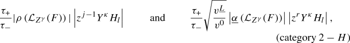
  where $j-1$, $r=\widetilde{N}-\kappa _P-(\beta ^1_l)_P$ and $r \le j$.

The terms of (category $2-H$) can only appear if $j=\widetilde{N}-\beta _P-(\beta ^1_i)_P$.

Proof

We merely sketch the proof as it is very similar to previous computations. One can express $T_F(\widehat{Z}^{\beta } H_i)$ using Lemma 9.1 and following what we did in the proof of Proposition 3.23. It then remains to copy the proof of Proposition 3.31 with $|\zeta _0|=0$, which explains that we do not have terms of (category 3). Note that $\max (|k|+1,|\gamma |) \le 8$ comes from Remark 9.2 and the fact that $|\kappa |$ can be equal to $|\beta |+1$ ensues from the transformation of the v derivative in the terms obtained from those of (type 2) and (type 3). $\square$

Remark 9.6

As $|\gamma | \le 8 \le N-3$, we have at our disposal pointwise decay estimates on the electromagnetic field (see Proposition (7.1)). Similarly, as $|k| \le 7 \le N-4$, Remark 7.8 gives us $|P_{k,p}(\Phi )| \lesssim \log ^{M_2}(1+\tau _+)$.

We are now ready to bound $\mathbb {E}^{\delta }_H$ and then to obtain estimates on $\int _v |z^j H_i|dv$.

Proposition 9.7

We have $\mathbb {E}^1_H +\mathbb {E}^0_H \lesssim \epsilon$ on [0, T[. Moreover, for $0 \le q \le 5$ and $|\beta | \le q$, we have for any $z \in \mathbf {k}_1$, $i \in I^{N-q}_1$, $j \le 2N-1-\beta _P-(\beta _i^1)_P$,

$$\begin{aligned} \forall \, (t,x) \in [0,T[ \times \mathbb {R}^3, \quad \int _v |z^j Y^{\beta } H_i| dv \lesssim \epsilon \frac{\log ^{2j+M_1}(3+t)}{\tau _+^2 \tau _-}. \end{aligned}$$

Proof

In the same spirit as Corollary 6.3 and in view of commutation formula of Lemma 9.5 (applied with $\widetilde{N} = 2N+3$) as well as the assumptions on $f_0$, there exists $C_H >0$ such that $\mathbb {E}^0_H(0) \le \mathbb {E}^1_H(0) \le C_H \epsilon$. We can prove that they both stay bounded by $3 C_H \epsilon$ by the continuity method. As it is very similar to what we did previously, we only sketch the proof. Consider $\delta \in \{ 0 , 1 \}$, $0 \le r \le 5$, $i \in I^{N-r}_1$, $|\beta | \le 3+r$, $z \in \mathbf {k}_1$ and $j \le 2N+2+\delta -\beta _P-(\beta ^1_i)_P$. The goal is to prove that

$$\begin{aligned} \int _0^t \int _{\Sigma _s} \int _v \left| T_F( z^j H_i ) \right| \frac{dv}{v^0}dxds \lesssim \epsilon ^{\frac{3}{2}} \log ^{j(\delta a+2)}(3+t). \end{aligned}$$

According to Lemma 9.5 (still applied with $\widetilde{N}=2N+3$), it is sufficient to obtain, if $\delta =1$, that the integral over $[0,t] \times \mathbb {R}^3_x \times \mathbb {R}^3_v$ of all terms of (category $0-H$)-(category $2-H$) are bounded by $\epsilon ^{\frac{3}{2}} \log ^{j( a+2)}(3+t)$. If $\delta =0$, we only have to deal with terms of (category $0-H$) and (category $1-H$) and to estimate their integrals by $\epsilon ^{\frac{3}{2}} \log ^{2j}(3+t)$. In view of Remark 9.6, we only have to apply (or rather follow the computations of) Propositions 8.1, 8.2 and 8.3. The pointwise decay estimates then ensue from the Klainerman–Sobolev inequality of Corollary 4.8. $\square$

Remark 9.8

A better decay rate, $\log ^{2j}(3+t) \tau _+^{-2} \tau _-^{-1}$, could be proved in the previous proposition by controling a norm analogous to $\mathbb {E}_N^{X}[f]$ but we do not need it to close the energy estimates on F.

Remark 9.9

We could avoid any hypothesis on the derivatives of order $N+1$ and $N+2$ of $F^0$ (see Subsection 17.2 of [10]).

9.2 The inhomogeneous part

As the matrix B in $T_F(G)+AG=BR^2$ contains top order derivatives of the electromagnetic field, we cannot commute the equation and prove $L^1$ estimates on $\widehat{Z} G$. Let us explain schematically how we will obtain an $L^2$ estimate on $\int _v |G|dv$ by recalling how we proceeded in [3]. We did not work with modified vector field and the matrices A and B did not hide v derivatives of G. Then we introduced K the solution of $T_F(K)+AK+KD=B$ which initially vanishes and where $T_F(R^2)=DR^2$. Thus $G=KR^2$ and we proved $\mathbb {E}[|K|^2 |R^2|] \le \epsilon$ so that the expected $L^2$ decay estimate followed from

$$\begin{aligned} \left\| \int _v |G|dv \right\| _{L^2_x} \lesssim \left\| \int _v |R^2| dv \right\| ^{\frac{1}{2}}_{L^{\infty }_x} \mathbb {E}[|K|^2 |R^2|]^{\frac{1}{2}}. \end{aligned}$$

The goal now is to adapt this process to our situation. There are two obstacles.

• The v derivatives hidden in the matrix A will then be problematic and we need first to transform them.

• The components of the (transformed) matrix A have to decay sufficiently fast. We then need to consider a larger vector valued field than G by including components such as $z^j G_i$ in order to take advantage of the hierarchies in the source terms already used before.

Recall from Definition 2.6 that we considered an ordering on $\mathbf {k}_1$ and that, if $\kappa$ is a multi-index, we have

$$\begin{aligned} z^{\kappa }= \prod _{i=1}^{|\kappa |} z_{\kappa _i} ~~\text {and} \quad |z^{\kappa }| \le \sum _{w \in \mathbf {k}_1} |w|^{|\kappa |}. \end{aligned}$$

In this section, we will sometimes have to work with quantities such as $z^{\kappa }$ rather than with $z^j$, where $j \in \mathbb {N}$.

Definition 9.10

Let I and $I^q$, for $N-5 \le q \le N$, be the sets

$$\begin{aligned}&I := \{ (\kappa , \beta ) \, / \, N-5 \le |\beta | \le N ~~ \text {and} ~~ |\kappa | \le N-\beta _P \} = \{ (\kappa _1,\beta _1),...,(\kappa _{|I|}, \beta _{|I|}) \},\\&I^q := \{ (\kappa , \beta ) \in I \, / \, |\beta |=q \}. \end{aligned}$$

Define now L, the vector valued fields of length |I|, such that

$$\begin{aligned} L_i = z^{\kappa _i} G_j, \quad \text {with} \quad \beta _j^1 = \beta _i, \quad \text {and} \quad [i]_I:=|\kappa _i|. \end{aligned}$$

Moreover, for $Y \in \mathbb {Y}$, $1 \le j \le |I_1|$ and $1 \le i \le |I|$, we define $j_Y$ and $i_Y$ the indices such that

$$\begin{aligned} R^1_{j_{Y}}=Y Y^{\beta ^1_j} f \quad \text {and} \quad L_{i_Y} = z^{\kappa _{i_Y}} G_{j_Y}. \end{aligned}$$

The following result will be useful for transforming the v derivatives.

Lemma 9.11

Let $Y \in \mathbb {Y}$ and $\beta ^1_i \in I_1 {\setminus } I^{N}_1$. Then

$$\begin{aligned} Y G_i = G_{i_Y}+H_{i_Y}-Y H_i. \end{aligned}$$

Proof

Recall that $R=H+G$ and remark that $Y R^1_i = Y Y^{\beta ^1_i} f= R^1_{i_Y}$. $\square$

We now describe the source terms of the equations satisfied by the components of L.

Proposition 9.12

There exists $N_1 \in \mathbb {N}^*$, a vector valued field W and three matrix-valued functions $\overline{A} : [0,T[ \times \mathbb {R}^3 \times \mathbb {R}^3 \rightarrow {\mathfrak {M}}_{|I|}(\mathbb {R})$, $\overline{B} : [0,T[ \times \mathbb {R}^3 \times \mathbb {R}^3 \rightarrow {\mathfrak {M}}_{|I|,N_1}(\mathbb {R})$, $\overline{D} : [0,T[ \times \mathbb {R}^3 \times \mathbb {R}^3 \rightarrow {\mathfrak {M}}_{N_1}(\mathbb {R})$ such that

$$\begin{aligned}&T_F(L)+\overline{A}L= \overline{B} W, \quad T_F(W)= \overline{D} W \quad \mathrm{and}\\&\quad \forall \, (t,x) \in [0,T[ \times \mathbb {R}^3, \quad \sum _{z \in \mathbf {k}_1} \int _v |z^{2} W| dv \lesssim \epsilon \frac{\log ^{3N+M_1} (3+t)}{\tau _+^2 \tau _-}. \end{aligned}$$

In order to depict these matrices, we use the quantity $[q]_W$, for $1 \le q \le N_1$, which will be defined during the construction of W in the proof. $\overline{A}$ and $\overline{B}$ are such that $T_F(L_i)$ can be bounded, for $1 \le i \le |I|$, by a linear combination of the following terms, where $|\gamma | \le 5$, $1 \le j,q \le |I|$ and $1 \le r \le N_1$.

where $p \le 2N$, $|k| \le N-1$ and $|k|+|\zeta | \le N$. Moreover, if $|k| \ge 6$, there exists $\kappa$ and $\beta$ such that $W_r = z^{\kappa } Y^{\beta } f$, $|k|+|\beta | \le N$ and $|\kappa | \le N+1-k_P-\beta _P$.

The matrix $\overline{D}$ is such that, for $1 \le i \le N_1$, $T_F(W_i)$ is bounded by a linear combination of the following expressions, where $|\gamma | \le N-5$ and $1 \le j,q \le N_1$.

Proof

The main idea is to transform the v derivatives in AG, following the proof of Lemma 3.28, and then to apply Lemma 9.11 in order to eliminate all derivatives of G in the source term of the equations. We then define W as the vector valued field, and $N_1$ as its length, containing all the following quantities

• $z^j Y^{\beta } f$,   with   $z \in \mathbf {k}_1$,   $|\beta | \le N-5$   and   $j \le N+1- \beta _P$,

• $z^j\left( H_{i_Y}-Y H_i \right)$,   with   $z \in \mathbf {k}_1$,   $Y \in \mathbb {Y}$,   $\beta _i^1 \in I_1 {\setminus } I_1^N$   and   $j \le N+3-\left( \beta ^1_{i_Y} \right) _P$.

• $z^j Y^{\beta } H_i$,   with   $z \in \mathbf {k}_1$,   $|\beta |+|\beta ^1_i| \le N$   and   $j \le N+3-\beta _P-(\beta ^1_i)_P$.

Let us make three remarks.

• If $1 \le i \le N_0$, we can define, in each of the three cases, $[i]_W:=j$.

• Including the terms $z^{N+1- \beta _P} Y^{\beta } f$ and $z^{N+1-\left( \beta ^1_{i_Y} \right) _P}\left( H_{i_Y}-Y H_i \right)$ in W allows us to avoid any term of category 2 related to $\overline{B}$.

• The components such as $z^j Y^{\beta } H_i$ are here in order to obtain an equation of the form $T_F(W)= \overline{D} W$.

The form of the matrix $\overline{D}$ then follows from Proposition 3.31 if $Y_i = z^j Y^{\beta } f$ and from Lemma 9.5, applied with $\widetilde{N}=N+3$, otherwise (we made an additional operation on the terms of category 0 which will be more detailed for the matrix $\overline{A}$). Note that we use Remark 7.8 to estimate all quantities such as $P_{k,p}(\Phi )$. The decay rate on $\int _v |z^2 W| dv$ follows from Proposition 8.11 and 9.7.

We now turn on the construction of the matrices $\overline{A}$ and $\overline{B}$. Consider then $1 \le i \le |I|$ and $1 \le q \le |I_1|$ so that $L_i=z^{\kappa _i} G_q$ and $|\kappa _i| \le N-(\beta ^1_q)_P$. Observe that

$$\begin{aligned} T_F(L_i)= T_F(z^{\kappa _i})G_q+z^{\kappa _i} T_F(G_q)= F \left( v, \nabla _v (z^{\kappa _i}) \right) G_q+z^{\kappa _i} T_F(G_q). \end{aligned}$$

The first term on the right hand side gives terms of (category $0-\overline{A}$) and (category $1-\overline{A}$) as, following the computations of Proposition 8.1, we have

$$\begin{aligned} \nabla _v \left( \prod _{r=1}^{|\kappa _i|} z_r \right)= & {} \sum _{p=1}^{|\kappa _i|} \nabla _v(z_p) \prod _{r \ne p} z_r,\\ \left| F(v,\nabla _v z_p) \right|\lesssim & {} \tau _- \left( |\rho (F) |+|\sigma (F) |+|\underline{\alpha }(F)| \right) +\tau _+ |\alpha (F)|+\sum _{w \in \mathbf {k}_1} |w F| . \end{aligned}$$

The remaining quantity, $z^{\kappa _i} T_F(G_q)=-z^{\kappa _i} A_q^r G_r+z^{\kappa _i} B_q^r R^2_r$, is described in Lemma 9.1. Express the terms given by $z^{\kappa _i} A_q^r G_r$ in null components and transform the v derivatives²⁷ of $G_r$ using Lemma 9.11, so that, schematically (see (27)),

$$\begin{aligned} v^0\left( \nabla _v G_r \right) ^r= & {} Y G_r+(t-r) \partial G_r\\= & {} G_{r_Y}+H_{r_Y}-Y H_r+(t-r)(G_{r_{\partial }}+H_{r_{\partial }}-\partial H_r) \quad \text {and} \quad \\ v^0 \partial _{v^b} G_r= & {} Y_{0b} G_r+x \partial G_r\\= & {} G_{r_{Y_{0b}}}+H_{r_{Y_{0b}}}-Y_{0b} H_r+x(G_{r_{\partial }}+H_{r_{\partial }}-\partial H_r) . \end{aligned}$$

By Remark 9.2, the $\Phi$ coefficients and the electromagnetic field are both derived less than 5 times. We then obtain, with similar operations as those made in proof of Proposition 3.31, the matrix $\overline{A}$ and the columns of the matrix $\overline{B}$ hitting the component of W of the form $z^j\left( H_{l_Y}-Y H_l \right)$. For $z^{\kappa _i} B_q^r R^2_r$, we refer to the proof of Proposition 3.31, where we already treated such terms. $\square$

To lighten the notations and since there will be no ambiguity, we drop the index I (respectively W) of $[i]_I$ for $1 \le i \le |I|$ (respectively $[j]_W$ for $1 \le j \le N_1$). Let us introduce K the solution of $T_F(K)+\overline{A}K+K\overline{D}=\overline{B}$, such as $K(0,.,.)=0$. Then, $KY= L$ since they are solution of the same system and they both initially vanish. The goal now is to control $\mathbb {E}[|K|^2|Y|]$. As, for $1 \le i \le |I|$ and $1 \le j,p \le N_1$,

$$\begin{aligned} T_F\left( |K^j_i|^2 W_p\right) = |K^j_i |^2\overline{D}^q_pW_q-2\left( \overline{A}^q_i K^j_q +K^q_i \overline{D}^j_q \right) K^j_i W_p+2\overline{B}^j_iK^j_iW_p, \end{aligned}$$

(84)

we consider $\mathbb {E}_L$, the following hierarchized energy norm,

$$\begin{aligned} \mathbb {E}_L(t):= \sum _{\begin{array}{c} 1 \le j,p \le N_1 \\ \, 1 \le i \le |I| \end{array}} \log ^{-4[i]-2[p]+4[j]}(3+t) \mathbb {E} \left[ \left| K_i^j\right| ^2 W_p \right] (t). \end{aligned}$$

The sign in front of [j] is related to the fact that the hierarchy is inversed on the terms coming from $K \overline{D}$. It prevents us to expect a better estimate than $\mathbb {E}_L(t) \lesssim \log ^{4N+12}(3+t)$.

Lemma 9.13

We have, for $M_0 = 4N+12$ and if $\epsilon$ small enough, $\mathbb {E}_L(t) \lesssim \epsilon \log ^{M_0}(3+t)$ for all $t \in [0,T[$.

Proof

We use again the continuity method. Let $T_0 \in [0,T[$ be the largest time such that $\mathbb {E}_L(t) \le 2 \epsilon \log ^{M_0}(3+t)$ for all $t \in [0,T_0[$ and let us prove that, if $\epsilon$ is small enough,

$$\begin{aligned} \forall \, t \in [0,T_0[, \quad \mathbb {E}_L(t) \lesssim \epsilon ^{\frac{3}{2}} \log ^{M_0}(3+t). \end{aligned}$$

(85)

As $T_0 >0$ by continuity (K vanishes initially), we would deduce that $T_0=T$. We fix for the remainder of the proof $1 \le i \le |I|$ and $1 \le j, p \le N_1$. According to the energy estimate of Proposition 4.1, (85) would follow if we prove that

$$\begin{aligned} I_{\overline{A}, \overline{D}}:= & {} \int _0^t \int _{\Sigma _s} \int _v \left| |K^j_i |^2 \overline{D}^q_pW_q-2\left( \overline{A}^k_i K^j_k +K^r_i \overline{D}^j_r \right) K^j_i W_p \right| \frac{dv}{v^0} dx ds \\\lesssim & {} \epsilon ^{\frac{3}{2}} \log ^{M_0+4[i]+2[p]-4[j]}(3+t), \\ I_{\overline{B}}:= & {} \int _0^t \int _{\Sigma _s} \int _v \left| B_i^j \right| \left| K^j_i W_p \right| \frac{dv}{v^0} dx ds \lesssim \epsilon ^{\frac{3}{2}}. \end{aligned}$$

Let us start by $I_{\overline{A}, \overline{D}}$ and note that in all the terms given by Proposition 9.12, the electromagnetic field is derived less than $N-5$ times so that we can use the pointwise decay estimates given by Remark 7.2. The terms of (category $1-\overline{A}$) and (category $1-\overline{D}$) can be easily handled (as in Proposition 8.2). We then only treat the following cases, where $|\gamma | \le N-5$ (the other terms are similar).

$$\begin{aligned}&\left| \overline{D}^j_r \right| = \tau _- \left( |\rho (F) |+|\sigma (F) |+|\underline{\alpha }(F)| \right) +\tau _+ |\alpha (F)|, \quad \text{ with } \quad [j]=[r]-1,\\ {}&\left| \overline{A}^k_i \right| \lesssim \frac{\tau _+ \sqrt{v^{\underline{L}}}}{\tau _- \sqrt{v^0}} |\underline{\alpha } (\mathcal {L}_{Z^{\gamma }}(F))|, \quad \text{ with } ~~[k] \le [i], \quad \text{ and } \\ {}&\left| \overline{D}^q_p \right| \lesssim \frac{\tau _+}{\tau _-} |\rho (\mathcal {L}_{Z^{\gamma }}(F))|, \quad \text{ with } ~~[q] < [p]. \end{aligned}$$

Without any summation on the indices r, k and q, we have, using Remark 7.2, $1 \lesssim \sqrt{v^0 v^{\underline{L}}}$ and the Cauchy-Schwarz inequality several times,

$$\begin{aligned} \int _0^t&\int _{\Sigma _s} \int _v \left| K^r_i \overline{D}^j_r K^j_i W_p \right| \frac{dv}{v^0} dx ds \\ {}&\quad \lesssim \sqrt{\epsilon } \int _0^t \frac{\log (3+s)}{1+s} \left| \mathbb {E}\left[ \left| K^r_i \right| ^2 W_p \right] \, (s) \, \mathbb {E}\left[ \left| K^j_i \right| ^2 W_p \right] \, (s) \right| ^{\frac{1}{2}} ds \\ {}&\quad \lesssim \epsilon ^{\frac{3}{2}} \log ^{2+M_0+4[i]+2[p]-2[r]-2[j]}(3+t) \lesssim \epsilon ^{\frac{3}{2}} \log ^{M_0+4[i]+2[p]-4[j]}(3+t), \\\int _0^t&\int _{\Sigma _s} \int _v \left| \overline{A}^k_i K^j_k K^j_i W_p\right| \frac{dv}{v^0} dx ds \\ {}&\quad \lesssim \sqrt{\epsilon }\int _{u=-\infty }^t \frac{\tau _+}{\tau _+\tau _-^{\frac{3}{2}}} \int _{C_u(t)} \int _v \frac{v^{\underline{L}}}{v^0} \left| K^j_k \right| \left| W_p\right| ^{\frac{1}{2}} \left| K^j_i \right| \left| W_p\right| ^{\frac{1}{2}} dv dC_u(t) du \\ {}&\quad \lesssim \sqrt{\epsilon } \left| \mathbb {E}\left[ \left| K^j_k \right| ^2 W_p \right] \, (t) \, \mathbb {E}\left[ \left| K^j_i \right| ^2 W_p \right] \, (t) \right| ^{\frac{1}{2}} \int _{u=-\infty }^{+\infty } \frac{du}{\tau _-^{\frac{3}{2}}} \\ {}&\quad \lesssim \epsilon ^{\frac{3}{2}} \log ^{M_0+2[k]+2[i]+2[p]-4[j]}(3+t) \lesssim \epsilon ^{\frac{3}{2}} \log ^{M_0+4[i]+2[p]-4[j]}(3+t), \\\int _0^t&\int _{\Sigma _s} \int _v \left| K^j_i \right| ^2 \left| \overline{D}^q_pW_q \right| \frac{dv}{v^0} dx ds \\ {}&\quad \lesssim \sqrt{\epsilon } \int _0^t \int _{\Sigma _s} \int _v \log (3+s) \frac{\sqrt{v^{\underline{L}}v^0}}{\tau _+^{\frac{1}{2}} \tau _-^{\frac{3}{2}}} \left| K^j_i \right| ^2 \left| W_q \right| \frac{dv}{v^0} dx ds \\ {}&\quad \lesssim \sqrt{\epsilon } \left( \int _0^t \frac{\log (3+s)}{1+s} ds+\log (3+t) \int _{-\infty }^{+\infty } \frac{du}{\tau _-^3} \right) \sup _{[0,t]} \, \mathbb {E}\left[ \left| K^j_i \right| ^2 W_q \right] \\ {}&\quad \lesssim \epsilon ^{\frac{3}{2}} \log ^{2+M_0+4[i]+2[q]-4[j]}(3+t) \lesssim \epsilon ^{\frac{3}{2}} \log ^{M_0+4[i]+2[p]-4[j]}(3+t). \end{aligned}$$

It remains to study $I_{\overline{B}}$. The form of $\overline{B}^j_i$ is given by Propoposition 9.12 and the computations are close to the ones of Proposition 8.7. We then only consider the following two cases,

$$\begin{aligned}&\left| \overline{B}^j_i K_i^j W_p \right| \lesssim \log ^{M_1}(1+\tau _+)\frac{\tau _+ \sqrt{v^{\underline{L}}}}{\tau _-\sqrt{v^0}} \left| \sigma (\mathcal {L}_{Z^{\zeta }} (F) ) \right| \left| K_i^j \right| |W_p|, \quad \text{ with } \quad |\zeta | \le N, \\ {}&\left| \overline{B}^j_i K_i^j W_p \right| \lesssim \left| \Phi ^r P_{\xi }(\Phi )|| \nabla _{ Z^{\gamma }} F \right| \left| K_i^j W_p \right| , \\&\quad \text{ with } \quad r \le 2N, \quad |\xi |+|\gamma | \le N \quad \text{ and } \quad 6 \le |\xi | \le N-1. \end{aligned}$$

In the first case, using a null foliation and the Cauchy-Schwarz inequality twice (in (t, x) and then in v), we get

$$\begin{aligned} I_{\overline{B}}\lesssim&{} \int _{-\infty }^t \! \left\| \sigma (\mathcal {L}_{Z^{\zeta }} (F) ) \right\| _{L^2(C_u(t))} \left| \int _{C_u(t)} \! \log ^{2M_1}(1+\tau _+)\frac{\tau _+^2}{\tau _-^2} \left| \int _v \sqrt{ \frac{v^{\underline{L}}}{v^0}} \left| K^j_i W_p \right| \frac{dv}{v^0} \right| ^2 \!dC_u(t) \right| ^{\frac{1}{2}}\! du \\\lesssim&{} \sqrt{\epsilon } \sum _{q=0}^{+ \infty } \int _{-\infty }^t \frac{1}{\tau _-^{\frac{5}{4}}} \left\| \tau _+^{\frac{11}{4}} \int _v \left| W_p \right| \frac{dv}{(v^0)^2} \right\| ^{\frac{1}{2}}_{L^{\infty }(C^q_u(t))} \left\| \int _v \frac{v^{\underline{L}}}{v^0} \left| K^j_i \right| ^2 \! \left| W_p \right| dv \right\| _{L^{1}(C^q_u(t))}^{\frac{1}{2}} \! du \\\lesssim&{} \epsilon ^{\frac{3}{2}} \int _{-\infty }^{+\infty } \frac{du}{\tau _-^{\frac{5}{4}}} \sum _{q=0}^{+\infty } \frac{\log ^{\frac{M_0+4[i]+2[p]+3N+M_1}{2}}(3+t_{q+1})}{(1+t_{q})^{\frac{1}{8}}} \lesssim \epsilon ^{\frac{3}{2}}, \end{aligned}$$

using the bootstrap assumption on $\mathbb {E}_L$ and $\int _v |W_p| \frac{dv}{(v^0)^2} \lesssim \int _v |W_p| \frac{v^{\underline{L}}}{v^0} dv \lesssim \epsilon \log ^{3N+M_1}(3+t) \tau _+^{-3}$, which comes from Proposition 9.12 and Lemma 3.2. For the remaining case, we have $|\gamma | \le N-6$ and we can then use the pointwise decay estimates on the electromagnetic field given by Proposition 7.1. Moreover, by Proposition 9.12, we have that

$$\begin{aligned} W_p = z^{\kappa } Y^{\beta } f , \quad \text {with} \quad |\xi |+|\beta | \le N \quad \text {and} \quad |\kappa | \le N+1-\beta _P-\xi _P. \end{aligned}$$

Suppose first that $|\kappa | \le 2N-1-\beta _P-2\xi _P$. Then, since $|\Phi |^r | \nabla _{Z^{\gamma }} F| \lesssim \sqrt{\epsilon } \tau _+^{-\frac{3}{4}}\tau _-^{-1}$ and $1 \lesssim \sqrt{v^0 v^{\underline{L}}}$, we get

$$\begin{aligned} \left| \overline{B}^j_i K^j_i W_p \right| \lesssim \sqrt{\epsilon } \left( \frac{v^0}{\tau _+^{\frac{5}{4}}}+\frac{v^{\underline{L}}}{\tau _+^{\frac{1}{4}} \tau _-^2} \right) \left( \left| z^{\kappa } P_{\xi }(\Phi )^2 Y^{\beta } f \right| +\left| K^j_i \right| ^2 \left| W_p \right| \right) . \end{aligned}$$

Hence, we can obtain $I_{\overline{B}} \lesssim \epsilon ^{\frac{3}{2}}$ by following the computations of Proposition 8.2, as, by the bootstrap assumptions on $\overline{\mathbb {E}}_N[f]$ and $\mathbb {E}_L$,

$$\begin{aligned} \mathbb {E}[ z^{\kappa } P_{\xi }(\Phi )^2 Y^{\beta } f ](t)+\mathbb {E}\left[ \left| K^j_i \right| ^2 W_p \right] (t) \lesssim \epsilon (1+t)^{\frac{1}{8}}. \end{aligned}$$

Otherwise, $|\kappa | = 2N-\beta _P-2\xi _P$ so that $\xi _P=N-1$, $|\beta | \le 1$ and $|\kappa | = 2-\beta _P$. We can then write $z^{\kappa }=z z^{\kappa _0}$ and find $q \in \llbracket 1,N_1 \rrbracket$ such that $W_q = z^2 z^{\kappa _0} Y^{\beta }f$. It remains to follow the previous case after noticing that

$$\begin{aligned}&\left| \overline{B}^j_i K^j_i W_p \right| \lesssim \sqrt{\epsilon } \left( \frac{v^0}{\tau _+^{\frac{5}{4}}}+\frac{v^{\underline{L}}}{\tau _+^{\frac{1}{4}} \tau _-^2} \right) \left( \left| z^{\kappa _0} P_{\xi }(\Phi )^2 Y^{\beta } f \right| +\left| K^j_i \right| ^2 \left| W_q \right| \right) ,\\ {}&|\kappa _0| \le 2N-1-2\xi _P-\beta _P. \end{aligned}$$

$\square$

9.3 $L^2$ estimates on the velocity averages of f

We finally end this section by proving several $L^2$ estimates. The first one is clearly not sharp but is sufficient for us to close the energy estimates for the electromagnetic field.

Proposition 9.14

Let $z \in \mathbf {k}_1$, $p \le 3N$, $|k| \le N-1$ and $\beta$ such that $|k|+|\beta | \le N$. Then, for all $t \in [0,T[$,

$$\begin{aligned} \left\| \frac{1}{\sqrt{\tau _+}} \int _v \left| zP_{k,p}(\Phi ) Y^{\beta }f \right| dv \right\| _{L^2 (\Sigma _t)}\lesssim & {} \frac{1}{1+t} \left\| \sqrt{\tau _+} \int _v \left| zP_{k,p}(\Phi ) Y^{\beta }f \right| dv \right\| _{L^2 (\Sigma _t)}\\\lesssim & {} \frac{\epsilon }{(1+t)^{\frac{5}{4}}} \end{aligned}$$

Proof

The first inequality ensues from $1+t \le \tau _+$ on $\Sigma _t$. For the other one, we start by the case $|\beta | \le N-3$. Write $P_{k,p}(\Phi )=\Phi ^n P_{\xi }(\Phi )$ and notice that $|\Phi |^n \lesssim \log ^{2p}(1+\tau _+)$. Then, using the bootstrap assumption (57) and Proposition 8.11,

$$\begin{aligned}&\left\| \sqrt{\tau _+} \int _v \left| z P_{k,p}(\Phi ) Y^{\beta }f \right| dv \right\| ^2_{L^2 (\Sigma _t)} \\ {}&\qquad \qquad \lesssim \left\| \tau _+ \log ^{4p}(1+\tau _+) \int _v \left| P_{\xi }(\Phi )^2 Y^{\beta }f \right| dv \int _v \left| z^2 Y^{\beta }f \right| dv \right\| _{L^{1} (\Sigma _t)} \\ {}&\qquad \qquad \lesssim \left\| \tau _+ \log ^{4p}(1+\tau _+) \int _v \left| z^2 Y^{\beta }f \right| dv \right\| _{L^{\infty } (\Sigma _t)} \overline{\mathbb {E}}_N[f](t) \\ {}&\qquad \qquad \lesssim \epsilon \frac{\log ^{4p+6}(3+t)}{1+t} (1+t)^{\eta } \lesssim \frac{\epsilon ^2}{(1+t)^{\frac{3}{4}}}. \end{aligned}$$

Otherwise, $|\beta | \ge N-2$ so that $|k| \le 2$ and, according to Remark 7.8, $P_{k,p}(\Phi ) \lesssim \tau _+^{\frac{1}{8}}$. Moreover, as there exists $i \in \llbracket 1, |I_1| \rrbracket$ such that $\beta =\beta ^1_i$, we obtain

$$\begin{aligned}&\left\| \tau _+^{\frac{1}{2}} \! \int _v \left| zP_{k,p}(\Phi ) Y^{\beta } \right| dv \right\| _{L^2 (\Sigma _t)} \lesssim \left\| \tau _+^{\frac{5}{8}} \! \int _v \left| z H_i \right| dv \right\| _{L^2 (\Sigma _t)}\!+\left\| \tau _+^{\frac{5}{8}} \! \int _v \left| z G_i \right| dv \right\| _{L^2 (\Sigma _t)}. \end{aligned}$$

Applying Proposition 9.7, one has

$$\begin{aligned} \left\| \tau _+^{\frac{5}{8}} \int _v \left| z H_i \right| dv \right\| ^2_{L^2 (\Sigma _t)} \lesssim&\left\| \tau _+^{\frac{5}{4}} \int _v \left| z^2 H_i \right| dv \right\| _{L^{\infty } (\Sigma _t)}\left\| \int _v \left| H_i \right| dv \right\| _{L^1 (\Sigma _t)} \\ \lesssim&\frac{\epsilon ^2}{(1+t)^{\frac{1}{2}}}. \end{aligned}$$

As there exists $q \in \llbracket 1, |I| \rrbracket$ such that $G_i=L_q=K_q^j W_j$, we have, using this time Proposition 9.13 and the decay estimate on $\int _v |z^2 W| dv$ given in Proposition 9.12,

$$\begin{aligned} \left\| \tau _+^{\frac{5}{8}} \int _v \left| z G_i \right| dv \right\| ^2_{L^2 (\Sigma _t)}= & {} \left\| \tau _+^{\frac{5}{8}} \int _v \left| z K_q^j W_j \right| dv \right\| ^2_{L^2 (\Sigma _t)} \\\lesssim & {} \sum _{j=0}^{N_1} \left\| \tau _+^{\frac{5}{4}} \int _v \left| z^2 W_j \right| dv \right\| _{L^{\infty } (\Sigma _t)} \left\| \int _v \left| K_q^j \right| ^2 \left| W_j \right| dv \right\| _{L^1 (\Sigma _t)} \\\lesssim & {} \epsilon \frac{\log ^{3N+M_1}(3+t)}{(1+t)^{\frac{3}{4}}}\log ^{4[q]}(3+t) \mathbb {E}_L(t) \lesssim \frac{\epsilon ^2}{(1+t)^{\frac{1}{2}}}. \end{aligned}$$

$\square$

This proposition allows us to improve the bootstrap assumption (58) if $\epsilon$ is small enough. More precisely, the following result holds.

Corollary 9.15

For all $t \in [0,T[$, we have $\sum _{|\beta | \le N-2} \left\| r^{\frac{3}{2}} \int _v \frac{v^A}{v^0} \widehat{Z}^{\beta } f dv \right\| _{L^2(\Sigma _t)} \lesssim \epsilon$.

Proof

Let $t \in [0,T[$. Using $\tau _+|v^A| \lesssim v^0 \sum _{z \in \mathbf {k}_1} |z|$ and rewritting $\widehat{Z}^{\beta }$ in terms of modified vector fields through the identity (38), one has for any $|\beta |\le N-2$

$$\begin{aligned} \left\| r^{\frac{3}{2}} \int _v \frac{v^A}{v^0} \widehat{Z}^{\beta } f dv \right\| _{L^2(\Sigma _t)} \lesssim \sum _{z \in \mathbf {k}_1} \sum _{p \le N-2} \sum _{\begin{array}{c} |q|+|\kappa | \le N-2 \\ |q| \le N-3 \end{array}} \left\| \sqrt{r} \int _v \left| P_{q,p}(\Phi ) Y^{\kappa } f \right| dv \right\| _{L^2(\Sigma _t)}\!. \end{aligned}$$

It then only remains to apply the previous proposition. $\square$

The two following estimates are crucial as a weaker decay rate would prevent us to improve the bootstrap assumptions.

Proposition 9.16

Let $\beta$ and $\xi$ such that $|\xi |+|\beta | \le N-1$. Then, for all $t \in [0,T[$,

$$\begin{aligned} \left\| \sqrt{\tau _-} \int _v \left| P^X_{\xi }(\Phi ) Y^{\beta } f \right| dv \right\| _{L^2(\Sigma _t)}\lesssim & {} \epsilon \frac{1}{1+t} \quad \text {if} \quad |\beta | \le N-3 \\\lesssim & {} \epsilon \frac{\log ^M(3+t)}{1+t} \quad \text {otherwise}. \end{aligned}$$

Proof

Suppose first that $|\beta | \le N-3$. Then, by Proposition 8.11,

$$\begin{aligned}&\left\| \sqrt{\tau _-} \int _v \left| P^X_{\xi }(\Phi ) Y^{\beta } f \right| dv \right\| ^2_{L^2(\Sigma _t)} \\ {}&\qquad \qquad \lesssim \left\| \tau _- \int _v \left| Y^{\beta } f \right| dv \right\| _{L^{\infty }(\Sigma _t)} \left\| \int _v \left| P^X_{\xi }(\Phi )^2 Y^{\beta } f \right| dv \right\| _{L^1(\Sigma _t)} \\ {}&\qquad \qquad \lesssim \frac{\epsilon }{(1+t)^2} \mathbb {E}^X_{N-1}[f](t) \lesssim \left| \frac{\epsilon }{1+t} \right| ^2 . \end{aligned}$$

Otherwise,

• $|\beta | \ge N-2$, so $|\xi | \le 1$ and then $|P^X_{\xi }(\Phi )| \lesssim \log ^{\frac{3}{2}} (1+\tau _+)$ by Proposition 7.6.

• There exists $i \in \llbracket 1, |I_1| \rrbracket$ and $q \in \llbracket 1, |I| \rrbracket$ such that $Y^{\beta } f = H_i+G_i=H_i+L_q$.

Using Proposition 9.7 (for the first estimate) and Propositions 9.12, 9.13 (for the second one), we obtain

$$\begin{aligned}&\left\| \sqrt{\tau _-} \int _v \left| P^X_{\xi }(\Phi ) H_i \right| dv \right\| ^2_{L^2(\Sigma _t)} \\&\quad ~~~~~~~~~~~~~~ \lesssim \left\| \tau _- \log ^{3}(1+\tau _+) \int _v \left| H_i \right| dv \right\| _{L^{\infty }(\Sigma _t)} \left\| \int _v \left| H_i \right| dv \right\| _{L^1(\Sigma _t)} \\&\quad ~~~~~~~~~~~~~~ \lesssim \left\| \epsilon \frac{\tau _- \log ^{3+M_1}(1+\tau _+)}{\tau _+^2 \tau _-} \right\| _{L^{\infty }(\Sigma _t)} \mathbb {E}[H_i](t) \lesssim \epsilon ^2 \frac{\log ^{3+M_1}(3+t)}{(1+t)^2}, \\&\left\| \sqrt{\tau _-} \int _v \left| P^X_{\xi }(\Phi ) L_q \right| dv \right\| ^2_{L^2(\Sigma _t)} \\&\quad ~~~~~~~~~~~~~~ = \left\| \sqrt{\tau _-} \int _v \left| P^X_{\xi }(\Phi ) K_q^j W_j \right| dv \right\| ^2_{L^2(\Sigma _t)} \\&\quad ~~~~~~~~~~~~~~ \lesssim \sum _{j=0}^{N_1} \left\| \tau _- \log ^{3}(1+\tau _+) \int _v \left| W_j \right| dv \right\| _{L^{\infty }(\Sigma _t)} \left\| \int _v \left| K_q^j \right| ^2 |W_j| dv \right\| _{L^1(\Sigma _t)} \\&\quad ~~~~~~~~~~~~~~ \lesssim \epsilon \frac{\log ^{3+3N+M_1}(3+t)}{(1+t)^2} \epsilon \log ^{M_0+4[q]}(3+t) \lesssim \epsilon ^2 \frac{\log ^{M_0+M_1+3N+3}(3+t)}{(1+t)^2}, \end{aligned}$$

since $[q]=0$. This concludes the proof if M is choosen such that²⁸$2M \ge M_0+M_1+3N+3$. $\square$

The following estimates will be needed for the top order energy norm. As it will be used combined with Proposition 3.40, the quantity $P_{q,p}(\Phi )$ will contain $\mathbb {Y}_X$ derivatives of $\Phi$.

Proposition 9.17

Let $\beta$, q and p be such as $|q|+|\beta | \le N$, $|q| \le N-1$ and $p \le q_X+\beta _T$. Then, for all $t \in [0,T[$,

$$\begin{aligned} \left\| \sqrt{\tau _-} \int _v \left| P_{q,p}(\Phi ) Y^{\beta } f \right| dv \right\| _{L^2(\Sigma ^0_t)} \lesssim \frac{\epsilon }{(1+t)^{1-\frac{\eta }{2}}}. \end{aligned}$$

Proof

We consider various cases and, except for the last one, the estimates are clearly not sharp. Let us suppose first that $|\beta | \ge N-2$. Then $|q| \le 2$ and $|P_{q,p}(\Phi )| \lesssim \log ^{M_1}(3+t)$ on $\Sigma ^0_t$ by Remark 7.8, so that, using Proposition 9.16,

$$\begin{aligned} \left\| \sqrt{\tau _-} \int _v \left| P_{k,p}(\Phi ) Y^{\beta } f \right| dv \right\| _{L^2(\Sigma ^0_t)}\lesssim & {} \log ^{M_1}(3+t) \left\| \sqrt{\tau _-} \int _v \left| Y^{\beta } f \right| dv \right\| _{L^2(\Sigma ^0_t)} \\\lesssim & {} \epsilon \frac{\log ^{M+M_1}(3+t)}{1+t}. \end{aligned}$$

Let us write $P_{q,p}(\Phi )=\Phi ^r P_{\xi }(\Phi )$ with $r \le p$ and $(\xi _T,\xi _P,\xi _X)=(q_T,q_P,q_X)$. If $|\beta | \le N-3$ and $|q| \le N-2$, then by the Cauchy-Schwarz inequality (in v), (83) as well as Propositions 7.6 and 8.11,

$$\begin{aligned}&\left\| \sqrt{\tau _-} \int _v \left| P_{k,p}(\Phi ) Y^{\beta } f \right| dv \right\| ^2_{L^2(\Sigma _t)} \\ {}&\qquad \qquad \lesssim \left\| \tau _- \int _v \left| \Phi ^{2r} Y^{\beta } f \right| dv \right\| _{L^{\infty }(\Sigma _t)} \left\| \int _v \left| P_{\xi }(\Phi )^2 Y^{\beta } f \right| dv \right\| _{L^1(\Sigma _t)} \\ {}&\qquad \qquad \lesssim \left\| \tau _-\frac{\epsilon \log ^{4r}(1+\tau _+)}{\tau _+^2\tau _-} \right\| _{L^{\infty }(\Sigma _t)}\mathbb {A}[f](t) \lesssim \epsilon ^2 \frac{\log ^{8N}(3+t)}{(1+t)^{2-\frac{3}{4}\eta }}. \end{aligned}$$

The remaining case is the one where $|q|=N-1$ and $|\beta | \le 1$. Hence, $p \le k_X+1$.

• If $p \ge 2$, we have $k_X \ge 1$ and then, schematically, $P_{\xi }(\Phi )=P^X_{\xi ^1}(\Phi ) P_{\xi ^2}(\Phi )$, with $|\xi ^1| \ge 1$ and $|\xi ^1|+|\xi ^2| = N-1$. If $|\xi ^2| \ge 1$, we have $\min (|\xi ^1|, |\xi ^2|) \le \frac{N-1}{2} \le N-6$ and one of the two factor can be estimated pointwise, which put us in the context of the case $|k| \le N-2$ and $|\beta | \le N-3$. Otherwise, $P_{k,p}(\Phi )= \Phi ^r P^X_{\xi ^1}(\Phi )$ and, using again (83),

  $$\begin{aligned}&\left\| \sqrt{\tau _-} \int _v \left| P_{k,p}(\Phi ) Y^{\beta } f \right| dv \right\| ^2_{L^2(\Sigma _t)} \\ {}&\qquad \qquad \lesssim \left\| \tau _- \int _v \left| \Phi ^{2r} Y^{\beta } f \right| dv \right\| _{L^{\infty }(\Sigma _t)} \left\| \int _v \left| P^X_{\xi ^1}(\Phi )^2 Y^{\beta } f \right| dv \right\| _{L^1(\Sigma _t)} \\ {}&\qquad \qquad \lesssim \left\| \tau _-\frac{\epsilon \log ^{4r}(1+\tau _+)}{\tau _+^2\tau _-} \right\| _{L^{\infty }(\Sigma _t)} \mathbb {A}[f](t) \lesssim \epsilon ^2 \frac{\log ^{8N}(3+t)}{(1+t)^{2-\frac{3}{4} \eta } }. \end{aligned}$$

• If $p=1$, we have $P_{k,p}(\Phi )=Y^{\kappa } \Phi$ and, using $\overline{\mathbb {E}}_N[f](t) \le 4 \epsilon (1+s)^{\eta }$,

  $$\begin{aligned}&\left\| \sqrt{\tau _-} \int _v \left| P_{k,p}(\Phi ) Y^{\beta } f \right| dv \right\| ^2_{L^2(\Sigma _t)} \\ {}&\qquad \qquad \lesssim \left\| \tau _- \int _v \left| Y^{\beta } f \right| dv \right\| _{L^{\infty }(\Sigma _t)} \left\| \int _v \left| Y^{\kappa } \Phi \right| ^2 \left| Y^{\beta } f \right| dv \right\| _{L^1(\Sigma _t)} \\ {}&\qquad \qquad \lesssim \left\| \tau _-\frac{\epsilon }{\tau _+^2\tau _-} \right\| _{L^{\infty }(\Sigma _t)} \mathbb {E}\left[ \left| Y^{\kappa } \Phi \right| ^2 Y^{\beta } f \right] (t) \lesssim \epsilon ^2 \frac{(1+t)^{\eta }}{(1+t)^2}. \end{aligned}$$

$\square$

10 Improvement of the Energy Estimates of the Electromagnetic Field

In order to take advantage of the null structure of the system, we start this section by a preparatory lemma.

Lemma 10.1

Let G be a 2-form and g a function, both sufficiently regular and recall that $J(g)^{\nu }= \int _v \frac{v^{\nu }}{v^0} g dv$, $\left| \overline{S}^{L} \right| \lesssim \tau _+$ and $\left| \overline{S}^{\underline{L}} \right| \lesssim \tau _-$. Then, using several times Lemma 2.4 and Remark 2.5,

$$\begin{aligned} \left| G_{ 0 \nu } J(g)^{\nu } \right| \lesssim&{} |\rho |\int _v |g|dv+(|\alpha _A|+|\underline{\alpha }_A| )\int _v \frac{|v^A|}{v^0}|g|dv \\\lesssim&{} |\rho |\int _v |g|dv+\frac{1}{\tau _+}\sum _{w \in \mathbf {k}_1}(|\alpha |+|\underline{\alpha }| )\int _v |wg|dv, \\ \left| \overline{S}^{\mu } G_{ \mu \nu } J(g)^{\nu } \right| \lesssim&{} \tau _+ |\rho | \int _v \frac{v^{\underline{L}}}{v^0} |g|dv+\tau _- |\rho | \int _v \frac{v^L}{v^0} |g|dv\\ {}&+\tau _+|\alpha |\int _v \frac{|v^A|}{v^0} |g| dv+\tau _-|\underline{\alpha }| \int _v \frac{|v^A|}{v^0}|g| dv \\\lesssim&{} \left( |\alpha |+|\rho |+ \frac{\tau _-}{\tau _+}|\underline{\alpha }| \right) \sum _{z \in \mathbf {k}_1} \int _v |z g | dv \quad \text{ if } |x| \ge t,\\\lesssim&{} |\rho | \int _v \left( \tau _-+\sum _{z \in \mathbf {k}_1} |z| \right) |g| dv+\left( |\alpha |+ \frac{\tau _-}{\tau _+}|\underline{\alpha }| \right) \sum _{z \in \mathbf {k}_1} \int _v |z g | dv \quad \text{ otherwise }. \end{aligned}$$

We are now ready to improve the bootstrap assumptions concerning the electromagnetic field.

10.1 For $\mathcal {E}^0_N[F]$

Using Proposition 4.3 and commutation formula of Proposition 3.40, we have, for all $t \in [0,T]$,

$$\begin{aligned} \mathcal {E}^0_N[F](t)-2\mathcal {E}^0_N[F](0) \lesssim \sum _{|\gamma | \le N} \sum _{\begin{array}{c} p \le |k|+|\beta | \le N \\ |k| \le N-1 \end{array}} \int _0^t \int _{\Sigma _s} |\mathcal {L}_{Z^{\gamma }}(F)_{\mu 0} J(P_{k,p}(\Phi ) Y^{\beta } f)^{\mu } | dx ds. \end{aligned}$$

(86)

We fix $|k|+|\beta | \le N$, $p \le N$ and $|\gamma | \le N$. Denoting the null decomposition of $\mathcal {L}_{Z^{\gamma }}(F)$ by $(\alpha , \underline{\alpha }, \rho , \sigma )$, $P_{k,p}(\Phi ) Y^{\beta } f$ by g and applying Lemma 10.1, one has

$$\begin{aligned}&\int _0^t \int _{\Sigma _s} |\mathcal {L}_{Z^{\gamma }}(F)_{\mu 0} J(P_{k,p}(\Phi ) Y^{\beta } f)^{\mu } | dx ds \\ {}&\qquad \qquad \lesssim \int _0^t \int _{\Sigma _s} |\rho | \int _v |g| dv +\left( |\alpha |+|\underline{\alpha }| \right) \sum _{w \in \mathbf {k}_1} \frac{1}{\tau _+} \int _v \left| w g \right| dv dx ds. \end{aligned}$$

On the one hand, using Proposition 9.14, there holds for any $w \in \mathbf {k}_1$,

$$\begin{aligned} \int _0^t \int _{\Sigma _s} \left( |\alpha |{+}|\underline{\alpha }| \right) \int _v \frac{1}{\tau _+} \left| w g \right| dv dx ds \lesssim \int _0^t \! \sqrt{\mathcal {E}^0_N[F](s)} \left\| \frac{1}{\tau _+} \int _v |wg| dv \right\| _{L^2(\Sigma _s)} \! ds \lesssim \epsilon ^{\frac{3}{2}}. \end{aligned}$$

On the other hand, as , we have

Since $\rho ( \mathcal {L}_{Z^{\gamma }}(\overline{F})) \lesssim \epsilon \tau _+^{-2}$ , we obtain, using Proposition 9.14 as well as the bootstrap assumptions (57), (60) and (63),

The right-hand side of (86) is then bounded by $\epsilon ^{\frac{3}{2}}$, implying that $\mathcal {E}^0_N[f] \le 3\epsilon$ on [0, T[ if $\epsilon$ is small enough.

10.2 The weighted norm for the exterior region

Applying Proposition 4.3 and using as well as , we have, for all $t \in [0,T[$,

Let us fix $|\gamma | \le N$ and denote the null decomposition of by $(\alpha , \underline{\alpha }, \rho , \sigma )$. As previously, using Proposition 3.40,

We fix $|k|+|\beta | \le N$, $p \le N$ and $|\gamma | \le N$ and we denote again $P_{k,p}(\Phi ) Y^{\beta } f$ by g. Using successively Lemma 10.1, the Cauchy-Schwarz inequality, the bootstrap assumption (60) and Proposition 9.14, we obtain

Using Proposition 5.1 and iterating commutation formula of Proposition 3.36, we have,

$$\begin{aligned} \tau _+^2\left| \nabla ^{\mu } {\mathcal {L}_{Z^{\gamma }}(\overline{F})_{\mu } }^{ L} \right| (t,x) +\tau _+^4\left| \nabla ^{\mu } {\mathcal {L}_{Z^{\gamma }}(\overline{F})_{\mu } }^{ \underline{L}} \right| (t,x) + \tau _+^3 \left| \nabla ^{\mu } {\mathcal {L}_{Z^{\gamma }}(\overline{F})_{\mu } }^{ A} \right| (t,x)&\\ \lesssim |Q(F)| \mathbb {1}_{-2 \le t-|x| \le -1}&(t,x). \end{aligned}$$

Consequently, as $|Q(F)| \le \Vert f_0 \Vert _{L^1_{x,v}} \le \epsilon$, $\left| \overline{S}^L \right| \lesssim \tau _+$ and $\left| \overline{S}^{\underline{L}} \right| \lesssim \tau _-$,

Note now that $\tau _- \mathbb {1}_{-2 \le t-|x| \le -1} \le \sqrt{5}$, so that, using the bootstrap assumption (60) and the Cauchy-Schwarz inequality,

Thus, if $\epsilon$ is small enough, we obtain on [0, T[ which improves the bootstrap assumption (60).

10.3 The weighted norms for the interior region

Recall from Proposition 4.3 that we have, for $Q \in \{ N-3, N-1, N \}$ and $t \in [0,T[$,

$$\begin{aligned} \mathcal {E}_Q[F](t) ~~ \le ~~ 24\epsilon +\sum _{|\gamma | \le Q} \int _0^t \int _{\Sigma ^0_s} \left| \overline{S}^{\mu } \mathcal {L}_{Z^{\gamma }}(F)_{\mu \nu } \nabla ^{\lambda } {\mathcal {L}_{Z^{\gamma }}(F)_{\lambda } }^{ \nu } \right| dx ds, \end{aligned}$$

(87)

since on [0, T[ by the bootstrap assumption (60)). The remainder of this subsection is divided in two parts. We consider first $Q \in \{ N-3, N-1 \}$ and we end with $Q=N$ as we need to use in that case a worst commutation formula in order to avoid derivatives of $\Phi$ of order N, which is the reason of the stronger loss on the top order energy norm.

10.3.1 The lower order energy norms

Let $Q \in \{ N-3, N-1 \}$. According to commutation formula of Proposition 3.39, we can bound the last term of (87) by a linear combination of the following ones.

$$\begin{aligned} \mathcal {I}_1:= & {} \int _0^t \int _{|x| \le s} \left| \overline{S}^{\mu } \mathcal {L}_{ Z^{\gamma }}(F)_{\mu \nu } \int _v \frac{v^{\nu }}{v^0} P^X_{\xi }(\Phi ) Y^{\beta } f dv \right| dx ds, \\&\qquad \text {with}\quad |\gamma | , \, |\xi |+|\beta | \le Q, \nonumber \end{aligned}$$

(88)

$$\begin{aligned} \mathcal {I}_2:= & {} \int _0^t \int _{|x| \le s} \left| \overline{S}^{\mu } \mathcal {L}_{ Z^{\gamma }}(F)_{\mu \nu } \int _v \frac{z}{\tau _+} P_{k,p}( \Phi ) Y^{\beta } f dv \right| dxds, \\&\qquad \text {with}\quad |\gamma | , \, |k|+|\beta | \le Q, \quad z \in \mathbf {k}_1,\nonumber \end{aligned}$$

(89)

$0 \le \nu \le 3$ and $p \le 3N$. Fix $|\gamma | \le Q$ and denote the null decomposition of $\mathcal {L}_{Z^{\gamma }}(F)$ by $(\alpha , \underline{\alpha }, \rho , \sigma )$. We start by (90), which can be estimated independently of Q. Recall that $\left| \overline{S}^{L} \right| \lesssim \tau _+$ and $\left| \overline{S}^{\underline{L}} \right| \lesssim \tau _-$, so that, using Proposition 9.14 and the bootstrap assumption (62),

$$\begin{aligned} \mathcal {I}_2\lesssim & {} \int _0^t \int _{\Sigma ^0_s} \left( \tau _+ |\rho |+\tau _+ |\alpha |+\tau _- |\underline{\alpha }| \right) \int _v \left| \frac{z}{\tau _+} P_{k,p}(\Phi ) Y^{\beta } f \right| dvdxds \\\lesssim & {} \int _0^t \sqrt{\mathcal {E}_{N-1}[F](s)} \left\| \frac{1}{\sqrt{\tau _+}} \int _v \left| z P_{k,p}( \Phi ) Y^{\beta } f \right| dv \right\| _{L^2(\Sigma _s)} ds \\\lesssim & {} \epsilon ^{\frac{3}{2}} \int _0^t \frac{\log ^M(3+s)}{(1+s)^{\frac{5}{4}}} ds \lesssim \epsilon ^{\frac{3}{2}}. \end{aligned}$$

We now turn on (89) and we then consider $|\xi |+|\beta | \le Q$. Start by noticing that, by Lemma 10.1,

$$\begin{aligned} \left| \overline{S}^{\mu } \mathcal {L}_{ Z^{\gamma }}(F)_{\mu \nu } \int _v \frac{v^{\nu }}{v^0} P^X_{\xi }(\Phi ) Y^{\beta } f \right| dv \lesssim&\tau _-|\rho | \int _v \left| P^X_{\xi }(\Phi ) Y^{\beta } f \right| dv \\&+\left( |\rho |+ |\alpha |+\frac{\tau _-}{\tau _+} |\underline{\alpha }| \right) \sum _{w \in \mathbf {k}_1} \int _v \left| w P^X_{\xi }(\Phi ) Y^{\beta } f \right| dv . \end{aligned}$$

Consequently, by the bootstrap assumption (62) and Proposition 9.14,

$$\begin{aligned} \mathcal {I}_1\lesssim&{} \int _0^t \sqrt{\mathcal {E}_{Q}[F](s)} \left\| \sqrt{\tau _-} \int _v \left| P^X_{\xi }(\Phi ) Y^{\beta } f \right| dv \right\| _{L^2(\Sigma _s)} \! ds \\&+ \sum _{w \in \mathbf {k}_1}\int _0^t \sqrt{\mathcal {E}_{Q}[F](s)} \left\| \frac{1}{\sqrt{\tau _+}} \int _v \left| w P^X_{\xi }(\Phi ) Y^{\beta } f \right| dv \right\| _{L^2(\Sigma _s)} \! ds \\\lesssim&{} \epsilon ^{\frac{3}{2}} + \int _0^t \sqrt{\mathcal {E}_{Q}[F](s)} \left\| \sqrt{\tau _-} \int _v \left| P^X_{\xi }(\Phi ) Y^{\beta } f \right| dv \right\| _{L^2(\Sigma _s)}ds. \end{aligned}$$

The last integral to estimate is the source of the small growth of $\mathcal {E}_Q[F]$. We can bound it, using again the bootstrap assumptions (61), (62) and Proposition 9.16, by

• $\epsilon ^{\frac{3}{2}} \log ^2(3+t)$ if $Q=N-3$ and

• $\epsilon ^{\frac{3}{2}} \log ^{2M}(3+t)$ otherwise.

Hence, combining this with (87) we obtain, for $\epsilon$ small enough, that

• $\mathcal {E}_{N-3}[F](t) \le 25 \epsilon \log ^2(3+t)$ for all $t \in [0,T[$ and

• $\mathcal {E}_{N-1}[F](t) \le 25 \epsilon \log ^{2M}(3+t)$ for all $t \in [0,T[$.

10.3.2 The top order energy norm

We consider here the case $Q=N$ and we then apply this time the commutation formula of Proposition 3.40, so that the last term of (87) can be bounded by a linear combination of terms of the form

$$\begin{aligned} \mathcal {I}:= \int _0^t \int _{\Sigma ^{0}_s} \left| \overline{S}^{\mu } \mathcal {L}_{Z^{\gamma }}(F)_{\mu \nu } \int _v \frac{v^{\mu }}{v^0} P_{q,p}(\Phi ) Y^{\beta } f dv \right| dx ds, \end{aligned}$$

with $|\gamma | \le N$, $|q|+|\beta | \le N$, $|q| \le N-1$ and $p \le q_X+\beta _T$. Let us fix such parameters. Following the computations made previously to estimate $\mathcal {I}_1$ and using $\mathcal {E}_{N}[F](s) \lesssim \sqrt{\epsilon } (1+s)^{\eta } \lesssim \sqrt{\epsilon } (1+s)^{\frac{1}{8}}$, we get

$$\begin{aligned} \mathcal {I}_1\lesssim&{} \int _0^t \sqrt{\mathcal {E}_{N}[F](s)} \left\| \sqrt{\tau _-} \int _v \left| P_{q,p}(\Phi ) Y^{\beta } f \right| dv \right\| _{L^2(\Sigma ^0_s)} \nonumber \\ {}&+ \sum _{w \in \mathbf {k}_1}\int _0^t \sqrt{\mathcal {E}_{N}[F](s)} \left\| \frac{1}{\sqrt{\tau _+}} \int _v \left| w P_{q,p}(\Phi ) Y^{\beta } f \right| dv \right\| _{L^2(\Sigma _s)} ds \nonumber \\\lesssim&{} \epsilon ^{\frac{3}{2}} + \sqrt{\epsilon } \int _0^t (1+s)^{\frac{\eta }{2}} \left\| \sqrt{\tau _-} \int _v \left| P_{q,p}(\Phi ) Y^{\beta } f \right| dv \right\| _{L^2(\Sigma ^0_s)}ds. \end{aligned}$$

(90)

Applying now Proposition 9.17, we can bound (90) by $\epsilon ^{\frac{3}{2}}(1+t)^{\eta }$. Thus, if $\epsilon$ is small enough, we obtain $\mathcal {E}_N[F](t) \le 25 \epsilon (1+t)^{\eta }$ for all $t \in [0,T[$, which concludes the improvement of the bootstrap assumption (63) and then the proof.

References

Andersson, L., Blue, P., Joudioux, J.: Hidden symmetries and decay for the Vlasov equation on the Kerr spacetime. Commun. Partial Differ. Equ. 43(1), 47–65 (2018)
Bieri, L., Miao, S., Shahshahani, S.: Asymptotic properties of solutions of the Maxwell Klein Gordon equation with small data. Comm. Anal. Geom. 25(1), 25–96 (2017)
Bigorgne, L.: Asymptotic properties of small data solutions of the Vlasov–Maxwell system in high dimensions (2017). arXiv:1712.09698
Bigorgne, L.: Sharp asymptotics for the solutions of the three-dimensional massless Vlasov–Maxwell system with small data (2018). arXiv:1812.09716
Bigorgne, L.: Asymptotic properties of the solutions to the Vlasov–Maxwell system in the exterior of a light cone (2019). arXiv:1902.00764
Bigorgne, L.: A vector field method for massless relativistic transport equations and applications. J. Funct. Anal. 108365 (2020). https://www.sciencedirect.com/science/article/pii/S0022123619303593
Christodoulou, D., Klainerman, S.: Asymptotic properties of linear field equations in Minkowski space. Commun. Pure Appl. Math. 43(2), 137–199 (1990)
Duan, X.: Sharp decay estimates for the Vlasov–Poisson and Vlasov–Yukawa systems with small data (2019). arXiv:1904.06176
Fajman, D., Joudioux, J., Smulevici, J.: Sharp asymptotics for small data solutions of the Vlasov–Nordström system in three dimensions (2017). arXiv:1704.05353
Fajman, D., Joudioux, J., Smulevici, J.: The Stability of the Minkowski space for the Einstein–Vlasov system (2017). arXiv:1707.06141
Fajman, D., Joudioux, J., Smulevici, J.: A vector field method for relativistic transport equations with applications. Anal. PDE 10(7), 1539–1612 (2017)
Glassey, R.T.: The Cauchy Problem in Kinetic Theory. Society for Industrial and Applied Mathematics (SIAM), Philadelphia (1996)
Glassey, R.T., Strauss, W.A.: Absence of shocks in an initially dilute collisionless plasma. Commun. Math. Phys. 113(2), 191–208 (1987)
Lindblad, H., Taylor, M.: Global stability of Minkowski space for the Einstein–Vlasov system in the harmonic gauge (2017). arXiv:1707.06079
Klainerman, S.: Uniform decay estimates and the Lorentz invariance of the classical wave equation. Commun. Pure Appl. Math. 38(3), 321–332 (1985)
Klainerman, S.: Remark on the asymptotic behavior of the Klein–Gordon equation in \({{ R}}^{n+1}\). Commun. Pure Appl. Math. 46(2), 137–144 (1993)
Lindblad, H., Rodnianski, I.: The global stability of Minkowski space–time in harmonic gauge. Ann. Math. (2) 171(3), 1401–1477 (2010)
Lindblad, H., Sterbenz, J.: Global stability for charged-scalar fields on Minkowski space. IMRP Int. Math. Res. Pap. pages Art. ID 52976, 109 (2006)
Schaeffer, J.: A small data theorem for collisionless plasma that includes high velocity particles. Indiana Univ. Math. J. 53(1), 1–34 (2004)
Shu, W.-T.: Global existence of Maxwell–Higgs fields. In: Nonlinear Hyperbolic Equations and Field Theory (Lake Como, 1990), Volume 253 of Pitman Res. Notes Math. Ser., pp. 214–227. Longman Scientific & Technical, Harlow (1992)
Smulevici, J.: Small data solutions of the Vlasov–Poisson system and the vector field method. Ann. PDE 2(2), Art. 11, 55 (2016)
Wang, X.: Propagation of regularity and long time behavior of the \(3D\) massive relativistic transport equation II: Vlasov–Maxwell system (2018). arXiv:1804.06566
Yang, S.: Decay of solutions of Maxwell–Klein–Gordon equations with arbitrary Maxwell field. Anal. PDE 9(8), 1829–1902 (2016)
Acknowledgements
Open access funding provided by Institute Mittag-Leffler. I am very grateful towards Jacques Smulevici, my Ph.D. advisor, for his support and for giving me precious advice. Part of this work was funded by the European Research Council under the European Union’s Horizon 2020 research and innovation program (project GEOWAKI, Grant Agreement 714408).
Author information
Authors and Affiliations
Corresponding author
Additional information
Communicated by W. Schlag
Publisher's Note
Springer Nature remains neutral with regard to jurisdictional claims in published maps and institutional affiliations.
Rights and permissions
Open Access This article is licensed under a Creative Commons Attribution 4.0 International License, which permits use, sharing, adaptation, distribution and reproduction in any medium or format, as long as you give appropriate credit to the original author(s) and the source, provide a link to the Creative Commons licence, and indicate if changes were made. The images or other third party material in this article are included in the article’s Creative Commons licence, unless indicated otherwise in a credit line to the material. If material is not included in the article’s Creative Commons licence and your intended use is not permitted by statutory regulation or exceeds the permitted use, you will need to obtain permission directly from the copyright holder. To view a copy of this licence, visit http://creativecommons.org/licenses/by/4.0/.
About this article
Cite this article
Bigorgne, L. Sharp Asymptotic Behavior of Solutions of the 3d Vlasov–Maxwell System with Small Data. Commun. Math. Phys. 376, 893–992 (2020). https://doi.org/10.1007/s00220-019-03604-3
Received:
Accepted:
Published:
Issue Date:
DOI: https://doi.org/10.1007/s00220-019-03604-3