Wilson lines and their Laurent positivity

Abstract

For a marked surface $\Sigma$ and a semisimple algebraic group G of adjoint type, we study the Wilson line morphism $g_{[c]}:{\mathcal {P} }_{G,\Sigma } \rightarrow G$ associated with the homotopy class of an arc c connecting boundary intervals of $\Sigma$, which is the comparison element of pinnings via parallel-transport. The matrix coefficients of the Wilson lines give a generating set of the function algebra $\mathcal {O}({\mathcal {P} }_{G,\Sigma })$ when $\Sigma$ has no punctures. The Wilson lines have the multiplicative nature with respect to the gluing morphisms introduced by Goncharov–Shen [18], hence can be decomposed into triangular pieces with respect to a given ideal triangulation of $\Sigma$. We show that the matrix coefficients $c_{f,v}^V(g_{[c]})$ give Laurent polynomials with positive integral coefficients in the Goncharov–Shen coordinate system associated with any decorated triangulation of $\Sigma$, for suitable f and v.

1 Introduction

The moduli space of G-local systems on a topological surface is a classical object of study, which has been investigated both from mathematical and physical viewpoints. Wilson loops give a class of important functions (or gauge-invariant observables), which are obtained as the traces of the monodromies of G-local systems in some finite-dimensional representations of G.

For a marked surface $\Sigma$, Fock–Goncharov [9] introduced two extensions ${\mathcal {A} }_{\widetilde{G},\Sigma }$ and ${\mathcal {X} }_{G,\Sigma }$ of the moduli space of local systems, each of which admits a natural cluster structure. Here $\widetilde{G}$ is a simply-connected semisimple algebraic group, and $G=\widetilde{G}/Z(\widetilde{G})$ is its adjoint group. The cluster structures of these moduli spaces are distinguished collections of open embeddings of algebraic tori accompanied with weighted quivers, related by two kinds of cluster transformations. The collection of weighted quivers is shared by ${\mathcal {A} }_{\widetilde{G},\Sigma }$ and ${\mathcal {X} }_{G,\Sigma }$, and thus they form a cluster ensemble in the sense of [11]. Such a cluster structure is first constructed by Fock–Goncharov [9] when the gauge groups are of type $A_n$, by Le [35] for type $B_n,C_n,D_n$ (and further investigated in [23]), and by Goncharov–Shen [18] for all semisimple gauge groups, generalizing all the works mentioned above and giving a uniform construction.

In [18], Goncharov–Shen introduced a new moduli space ${\mathcal {P} }_{G,\Sigma }$ closely related to the moduli space ${\mathcal {X} }_{G,\Sigma }$, which possesses the frozen coordinates that are missed in the latter. When $\partial \Sigma =\emptyset$, we have ${\mathcal {P} }_{G,\Sigma }={\mathcal {X} }_{G,\Sigma }$, and otherwise the former includes additional data called the pinnings assigned to boundary intervals. The supplement of frozen coordinates turns out to be crucial in the quantum geometry of moduli spaces: for example, it is manifestly needed in the relation with the quantized enveloping algebra in their work. The data of pinnings also allow one to glue the G-local systems along boundary intervals in an unambiguous way, which leads to a gluing morphism

$$\begin{aligned} q_{E_1,E_2}: {\mathcal {P} }_{G,\Sigma } \rightarrow {\mathcal {P} }_{G,\Sigma '}. \end{aligned}$$

Here $\Sigma '$ is obtained from $\Sigma$ by gluing two boundary intervals $E_1$ and $E_2$ of $\Sigma$.

1.1 The Wilson lines

Using the data of pinnings, we introduce a new class of G-valued morphisms

$$\begin{aligned} g_{[c]}: {\mathcal {P} }_{G,\Sigma } \rightarrow G, \end{aligned}$$

which we call the Wilson line along the homotopy classes [c] of a curve connecting two boundary intervals called an arc class. Roughly speaking, the Wilson line $g_{[c]}$ is defined to be the comparison element of the two pinnings assigned to the initial and terminal boundary intervals under the parallel-transport along the curve c. Our aim in this paper is a detailed study of these morphisms. Here are main features:

Multiplicativity:

We will see that the Wilson lines have the multiplicative nature for the gluing morphisms. If we have two arc classes $[c_1]:E_1 \rightarrow E_2$ and $[c_2]:E'_2 \rightarrow E_3$ on $\Sigma$, then by gluing the boundary intervals $E_2$ and $E'_2$ we obtain another marked surface $\Sigma '$ equipped with an arc class $[c]:=[c_1]*[c_2]$, which is the concatenation of the two arcs. Then we will see that the Wilson line $g_{[c]}$ is given by the product of the Wilson lines $g_{[c_1]}$ and $g_{[c_2]}$. See Proposition 3.11 and Fig. 3.

Open analogue of Wilson loops:

Let

$$\begin{aligned} \rho _{|\gamma |}:{\mathcal {P} }_{G,\Sigma } \rightarrow [G/{{\,\mathrm{{\textrm{Ad}}}\,}}G] \end{aligned}$$

be the morphism given by the monodromy along a free loop $|\gamma |$, which we call the Wilson loop in this paper¹. Using the multiplicativity above, one can compute the Wilson loop from the Wilson line along the arc obtained by cutting the loop $\gamma$ along an edge. See Proposition 3.12 and Fig. 4. In this sense, the Wilson lines are “open analogues” of the Wilson loops.

Generation of the function algebra:

The matrix coefficients of Wilson lines give rise to regular functions on ${\mathcal {P} }_{G,\Sigma }$. Moreover, we will see in Sect. 3.4 that the function algebra $\mathcal {O}({\mathcal {P} }_{G,\Sigma })$ is generated by these matrix coefficients when $\Sigma$ has no punctures. Therefore Wilson lines provide enough functions to study the function algebra $\mathcal {O}({\mathcal {P} }_{G,\Sigma })$.

Universal Laurent property:

Shen [40] proved that the algebra $\mathcal {O}({\mathcal {P} }_{G,\Sigma })$ of regular functions on this moduli stack is isomorphic to the cluster Poisson algebra $\mathcal {O}_{\textrm{cl}}({\mathcal {P} }_{G,\Sigma })$, which is by definition the algebra of regular functions on the corresponding cluster Poisson variety. Hence the matrix coefficients of Wilson lines belong to $\mathcal {O}_{\textrm{cl}}({\mathcal {P} }_{G,\Sigma })$. In other words, they are universally Laurent polynomials, meaning that they are expressed as Laurent polynomials in any cluster chart (including those not coming from decorated triangulations).

We remark here that the essential notion of Wilson lines has been appeared in many related works including [4, 9, 13, 18, 19, 39] (mainly as a tool for the computation of Wilson loops), while our work would be the first on its systematic study in the setting of the moduli space ${\mathcal {P} }_{G,\Sigma }$. Via their coordinate expressions as we discuss below, the Wilson lines (loops) have been recognized as related to the spectral networks [13] and certain integrable systems [39].

1.2 Laurent positivity of Wilson lines

Our goal in this paper is a detailed study of the Laurent expressions of the matrix coefficients of Wilson lines in cluster charts on ${\mathcal {P} }_{G,\Sigma }$. Moreover, it will turn out that a special class of matrix coefficients give rise to Laurent polynomials with non-negative coefficients.

Fock–Goncharov’s snake formula. Coordinate expressions of Wilson loops (or the trace functions) have been studied by several authors. In the $A_1$ case, a combinatorial formula for the expressions of Wilson loops in terms of the cross ratio coordinates is given by Fock [8] (see also [7, 36]). It expresses the Wilson loop along a free loop $|\gamma |$ as a product of the elementary matrices

$$\begin{aligned} L=\begin{pmatrix}1 &{}\quad 1\\ 0 &{}\quad 1 \end{pmatrix},\quad R=\begin{pmatrix}1 &{}\quad 0\\ 1 &{}\quad 1 \end{pmatrix},\quad H(x)=\begin{pmatrix}x^{1/2} &{}\quad 0\\ 0 &{}\quad x^{-1/2}\end{pmatrix}\quad \in PGL_2, \end{aligned}$$

which are multiplied according to the turning pattern after substituting the cross ratio coordinates into x.

In the $A_n$ case, Fock–Goncharov [6] gave a similar formula called the snake formula, which expresses the Wilson loops in the cluster coordinates associated with ideal triangulations (called the special coordinate systems). In particular, the trace functions are positive Laurent polynomials (with fractional powers) in any special coordinate systems.

Generalizations of the snake formula. Generalizing the special coordinate systems, Goncharov–Shen [18] gave a uniform construction of coordinate systems on ${\mathcal {P} }_{G,\Sigma }$ associated with decorated triangulations.² Let us call them the Goncharov–Shen coordinate systems (GS coordinate systems for short). The special coordinate systems in the type $A_n$ case are special instances of the GS coordinate systems, where the choice of reduced words are the “standard” one (see (4.8)). Unlike the special coordinate systems, however, a general GS coordinate system no longer have the cyclic symmetry on each triangle. The data of “directions” of coordinates is encoded in the data of decorated triangulations, as well as the choice of reduced words on each triangle.

Locally, a natural generalization of the snake formula is given by the evaluation map [6] parametrizing the double Bruhat cells of G. We will see that the “basic” Wilson lines $b_L,b_R$ on the configuration space ${\textrm{Conf}}_3 {\mathcal {P} }_G$,which models the moduli space on the triangle, can be expressed using the evaluation maps. Since the multiplicativity allows one to decompose Wilson lines into those on triangles, one can write the Wilson lines as a product of evaluation maps when the direction of GS coordinates agree with the direction that the arc class traverses on each triangle. This is basically the same strategy as Fock–Goncharov [6], but manipulations in the recently-innovated moduli space ${\mathcal {P} }_{G,\Sigma }$ makes the computation much clearer, thanks to the nice properties of the gluing morphism [18].

Transformations by cyclic shifts. In general, we need to transform the evalutation maps in the expression of Wilson lines by the cyclic shift automorphism on ${\textrm{Conf}}_3 {\mathcal {P} }_G$, in order to match the directions of a given GS coordinate system with the direction of the arc class on each triangle. The cyclic shifts are known to be written as a composite of cluster transformations, which is computable in nature but rather a complicated rational transformation. While the matrix coefficients of $g_{[c]}$ are at least guaranteed to be Laurent polynomials as we discussed above, it is therefore non-trivial whether their coefficients are non-negative integers.

Let us further clarify the problem which we will deal with. A function $f \in \mathcal {O}({\mathcal {P} }_{G,\Sigma })$ is said to be GS-universally positive Laurent if it is expressed as a Laurent polynomial with non-negative integral coefficients in the GS coordinate system associated with any decorated triangulation $\varvec{\Delta }$. This is a straightforward generalization of special good positive Laurent polynomials on ${\mathcal {X} }_{PGL_{n+1},\Sigma }$ in [9]. Moreover, a morphism $F: {\mathcal {P} }_{G,\Sigma }\rightarrow G$ is said to be GS-universally positive Laurent if for any finite-dimensional representation V of G, there exists a basis $\mathbb {B}$ of V such that

$$\begin{aligned} F^*c_{f, v}^V \in \mathcal {O}({\mathcal {P} }_{G,\Sigma }) \end{aligned}$$

is GS-universally positive Laurent for all $v\in \mathbb {B}$ and $f\in \mathbb {F}$, where $\mathbb {F}$ is the basis of $V^{*}$ dual to $\mathbb {B}$. Our result is the following:

Theorem 1

(Theorem 5.2) Let G be a semisimple algebraic group of adjoint type, and assume that our marked surface $\Sigma$ has non-empty boundary. Then, for any arc class $[c]:E_\textrm{in}\rightarrow E_\textrm{out}$, the Wilson line $g_{[c]}: {\mathcal {P} }_{G,\Sigma }\rightarrow G$ is a GS-universally positive Laurent morphism.

Since the Wilson loops $\rho _{|\gamma |}: {\mathcal {P} }_{G,\Sigma } \rightarrow [G/{{\,\mathrm{{\textrm{Ad}}}\,}}G]$ can be computed from the Wilson lines by Proposition 3.12, it immediately implies the following:

Corollary 2

(Corollary 5.3) Let G be a semisimple algebraic group of adjoint type, and $|\gamma | \in \widehat{\pi }(\Sigma )$ a free loop. Then, for any finite dimensional representation V of G, the trace function $\mathop {\textrm{tr}}\nolimits _V(\rho _{|\gamma |}):=\rho _{|\gamma |}^*\mathop {\textrm{tr}}\nolimits _V \in \mathcal {O}({\mathcal {P} }_{G,\Sigma })$ is GS-universally positive Laurent.

Corollary 2 is a generalization of [9, Theorem 9.3, Corollary 9.2].

Here we briefly comment on the proof of Corollary 1. By the construction of the GS coordinate system on ${\mathcal {P} }_{G,\Sigma }$ associated with a decorated triangulation, the Laurent positivity of a regular function on ${\mathcal {P} }_{G,\Sigma }$ can be deduced from the Laurent positivity of its pull-back via the gluing morphism $q_\Delta : \prod _{T \in t(\Delta )} {\mathcal {P} }_{G,T}\rightarrow {\mathcal {P} }_{G,\Sigma }$ associated with the underlying ideal triangulation $\Delta$. In other words, we can investigate the Laurent positivity of a regular function on ${\mathcal {P} }_{G,\Sigma }$ by a local argument on triangles. Indeed, a key to the proof of Corollary 1 is a construction of a basis $\widetilde{\mathbb {F}}_{\textrm{pos}, T}$ of $\mathcal {O}({\mathcal {P} }_{G,T})$ consisting of GS-universally positive Laurent elements, which is invariant under the cyclic shift and compatible with certain matrix coefficients.

We show that such a nice basis is constructed whenever we have a nice basis $\mathbb {F}_{\textrm{pos}}$ of the coordinate ring $\mathcal {O}(U^+_{*})$ of the unipotent cell $U^+_{*}$ of G. In particular, the invariance of $\widetilde{\mathbb {F}}_{\textrm{pos}, T}$ under the cyclic shift on ${\mathcal {P} }_{G,T}$ comes from the invariance of $\mathbb {F}_{\textrm{pos}}$ under the Berenstein-Fomin-Zelevinsky twist automorphism on $U^+_{*}$ [1, 2]. An example of a basis of $\mathcal {O}(U^+_{*})$ which satisfies the list of desired properties (see Theorem 5.7) is obtained from the theory of categorification of $\mathcal {O}(U^{+}_{*})$ via quiver Hecke algebras, which has been investigated, for example, in [28,29,30,31,32,33, 37, 38].

The GS-universally positive Laurent property is weaker than the universal positive Laurent property [11], which requires a similar positive Laurent property for all cluster charts. By replacing the GS-universally positive Laurent property with universal positive Laurent property, we have the notion of universally positive Laurent morphisms. Then, it would be natural to expect the following:

Conjecture 3

For any arc class $[c]:E_\textrm{in}\rightarrow E_\textrm{out}$, the Wilson line $g_{[c]}: {\mathcal {P} }_{G,\Sigma }\rightarrow G$ is a universally positive Laurent morphism. Moreover, the trace function $\mathop {\textrm{tr}}\nolimits _V(\rho _{|\gamma |}) \in \mathcal {O}({\mathcal {P} }_{G,\Sigma })$ is universally positive Laurent.

Indeed, it is known that this conjecture on the trace functions holds true for type $A_1$ case [9]. In our continuing work [24] with Linhui Shen, it is shown that the generalized minors of Wilson lines are cluster monomials. In particular, they are known to be universally positive Laurent [21].

1.3 Future directions

1.3.1 Poisson brackets of Wilson lines

The absolute values $|\mathop {\textrm{tr}}\nolimits _V(\rho _{|\gamma |})|$ of the trace functions in the vector representation are well-defined smooth functions on the positive-real part ${\mathcal {P} }_{G,\Sigma }(\mathbb {R}_{>0})$ (or ${\mathcal {X} }_{G,\Sigma }(\mathbb {R}_{>0})$), in spite of the fact that V is not a representation of the adjoint group G. In the type $A_n$ case, Chekhov–Shapiro [4] proved that the cluster Poisson brackets of these functions reproduce the Goldman brackets [16]. Their argument is local in nature and seems to be applicable also to Wilson lines, and it can be expected that (absolute values of) certain matrix coefficients of the Wilson lines form an open analogue of the Goldman algebra.

1.3.2 Quantum lifts of Wilson lines

Any cluster Poisson variety ${\mathcal {X} }$ admits a canonical quantization, namely a one-parameter deformation $\mathcal {O}_q({\mathcal {X} })$ of the cluster Poisson algebra $\mathcal {O}({\mathcal {X} })$ and its representation on a certain Hilbert space as self-adjoint operators [10]. It will be an interesting problem to consider a quantum analogue of the matrix coefficients of the Wilson lines, which belong to $\mathcal {O}_q({\mathcal {P} }_{G,\Sigma })$ and recovers $c^V_{f,v}(g_{[c]})$ in the classical limit $q\rightarrow 1$. A special example is the Goncharov–Shen’s realization of the quantum enveloping algebra $U_q(\mathfrak {b}^+)$ inside the quantum cluster Poisson algebra [18, Section 11], whose generators are quantum lifts of certain matrix coefficients of the Wilson line along an arc class that encircles exactly one special point (see Lemma 3.14). In the type $A_n$ case, quantum lifts are also studied by Douglas [5] and Chekhov–Shapiro [4].

A comparison with the quantization of the moduli stacks in terms of the factorization homology studied by [26] will also be an important problem.

1.4 Organization of the paper

Geometric study of Wilson lines (Sects. 2, 3) After recalling basic notations in Sect. 2, we introduce the Wilson line morphisms in Sect. 3 and study their properties from the geometric point of view. Some basic facts on the quotient stacks are summarized in Sect. 1. In Sect. 3.4, we prove the generation of the function algebra $\mathcal {O}({\mathcal {P} }_{G,\Sigma })$ by the matrix coefficients of Wilson lines when $\Sigma$ has no punctures. We give the decomposition formulae for the Wilson lines in Sect. 3.5.4, as a preparation for the study on the coordinate expressions. Coordinate expressions and Laurent positivity (Sects. 4, 5) After recalling the Goncharov–Shen coordinates on the moduli space ${\mathcal {P} }_{G,\Sigma }$ and relevant coordinate systems on unipotent cells and double Bruhat cells in Sect. 4, we study we study the coordinate expressions of the Wilson lines and prove Corollary 1 in Sect. 5. In the course of the proof, we construct a basis of $\mathcal {O}({\mathcal {P} }_{G,T})$ for a triangle T consisting of GS-universally positive Laurent elements, which is invariant under the cyclic shift. Some basic notions on the cluster varieties, weighted quivers and their amalgamation procedure are recollected in Appendix B.

2 Configurations of pinnings

Denote by $\mathbb {G}_m={{\,\mathrm{\textrm{Spec}}\,}}{\mathbb C}[t,t^{-1}]$ the multiplicative group scheme over ${\mathbb C}$. For an algebraic torus T over ${\mathbb C}$, let $X^*(T):=\mathop {\textrm{Hom}}\nolimits (T,\mathbb {G}_m)$ be the lattice of characters, $X_*(T):=\mathop {\textrm{Hom}}\nolimits (\mathbb {G}_m, T)$ the lattice of cocharacters, and $\langle -,-\rangle$ the natural pairing

$$\begin{aligned} \langle -,-\rangle :~ X_*(T)\times X^*(T)\longrightarrow \mathop {\textrm{Hom}}\nolimits (\mathbb {G}_m, \mathbb {G}_m)\simeq {\mathbb Z}. \end{aligned}$$

For $t\in T$ and $\mu \in X^*(T)$, the evaluation of $\mu$ at t is denoted by $t^{\mu }$.

2.1 Notations from Lie theory

In this subsection, we briefly recall basic terminologies in Lie theory. See [25] for the details.

Let $\widetilde{G}$ be a simply-connected connected simple algebraic group over $\mathbb {C}$. Let $\widetilde{B}^+$ be a Borel subgroup of $\widetilde{G}$ and $\widetilde{H}$ a maximal torus (a.k.a. Cartan subgroup) contained in $\widetilde{B}^+$, respectively. Let $U^+$ be the unipotent radical of $\widetilde{B}^+$. Let

• $X^*(\widetilde{H})$ be the weight lattice and $X_*(\widetilde{H})$ the coweight lattice;

• $\Phi \subset X^*(\widetilde{H})$ the root system of $(\widetilde{G}, \widetilde{H})$;

• $\Phi _+\subset \Phi$ the set of positive roots consisting of the $\widetilde{H}$-weights of the Lie algebra of $U^+$;

• $\{\alpha _s\mid s\in S\}\subset \Phi _+$ the set of simple roots, where S is the index set with $|S|=r$;

• $\{\alpha _s^\vee \mid s \in S\} \subset X_*(\widetilde{H})$ the set of simple coroots.

For $s\in S$, let $\varpi _s\in X^*(\widetilde{H})$ be the s-th fundamental weight defined by $\langle \alpha _t^{\vee }, \varpi _s\rangle =\delta _{st}$. Then we have $\alpha _t=\sum _{u \in S} C_{ut} \varpi _u$ for $t \in S$, where $C_{st}:=\langle \alpha _s^\vee , \alpha _t\rangle \in \mathbb {Z}$. We have

$$\begin{aligned} X^*(\widetilde{H})=\sum _{s\in S}\mathbb {Z}\varpi _s \quad \text{ and }\quad X_*(\widetilde{H})=\sum _{s\in S}\mathbb {Z}\alpha ^\vee _s. \end{aligned}$$

The sub-lattice generated by $\alpha _s$ for $s\in S$ is called the root lattice.

For $s\in S$, we have a pair of root homomorphisms $x_{s}, y_{s}:\mathbb {A}^1\rightarrow \widetilde{G}$ such that

$$\begin{aligned} hx_{s}(t)h^{-1}=x_{s}(h^{\alpha _s}t), \qquad hy_s(t)h^{-1}=y_s(h^{-\alpha _s}t) \end{aligned}$$

for $h\in \widetilde{H}$. After a suitable normalization, we obtain a homomorphism $\varphi _{s}:SL_2\rightarrow \widetilde{G}$ such that

$$\begin{aligned} \varphi _{s}\left( \begin{pmatrix} 1&{}\quad a\\ 0&{}\quad 1 \end{pmatrix}\right) =x_{s}(a), \qquad \varphi _{s} \left( \begin{pmatrix} 1&{}\quad 0\\ a&{}\quad 1 \end{pmatrix}\right) = y_s(a), \qquad \varphi _{s} \left( \begin{pmatrix} a&{}\quad 0\\ 0&{}\quad a^{-1} \end{pmatrix}\right) = \alpha _s^\vee (a). \end{aligned}$$

The group $G=\widetilde{G}/Z(\widetilde{G})$ is called the adjoint group, where $Z(\widetilde{G})$ denotes the center of $\widetilde{G}$. Then $B^+:=\widetilde{B}^+/Z(\widetilde{G})$ is a Borel subgroup of G and $H:=\widetilde{H}/Z(\widetilde{G})$ is a Cartan subgroup of G. Moreover the unipotent radical of $B^+$ is isomorphic to $U^+$ through the natural map $\widetilde{G}\rightarrow G$, which we again denote by $U^+$. Then we have $B^+=HU^+$. The natural map $\widetilde{H}\rightarrow H$ induces ${\mathbb Z}$-module homomorphisms

$$\begin{aligned} X^*(H)=\sum _{s\in S}\mathbb {Z}\alpha _s \hookrightarrow X^*(\widetilde{H}) \quad \text{ and }\quad X_*(\widetilde{H})\twoheadrightarrow X_*(H)=\sum _{s\in S}\mathbb {Z}\varpi ^\vee _s, \end{aligned}$$

where $\varpi _s^\vee \in X_*(H)$ is the s-th fundamental coweight defined by $\langle \varpi _s^{\vee }, \alpha _t\rangle =\delta _{st}$; we tacitly use the same notations for the elements related by these maps. The above mentioned one-parameter subgroups $x_s, y_s$ descend to the homomorphisms $x_{s}, y_{s}:\mathbb {A}^1\rightarrow G$ with the same notation. There exists an anti-involution

$$\begin{aligned} \textsf{T}:G\rightarrow G,\ g\mapsto g^\textsf{T} \end{aligned}$$

of the algebraic group G given by $x_s(t)^\textsf{T}=y_s(t)$ and $h^\textsf{T}=h$ for $s\in S, t\in \mathbb {A}^1, h\in H$. This is called the transpose in G. Let

• $B^-:=(B^+)^\textsf{T}$ be the opposite Borel subgroup of $B^+$, and $U^-:=(U^+)^\textsf{T}$;

• $G_0:=U^-HU^+ \subset G$ the open subvariety of triangular-decomposable elements.

Definition 1.1

In G, define $\mathbb {E}^s:=x_s(1) \in U^+$ and $\mathbb {F}^s:=y_s(1) \in U^-$ for each $s \in S$. Let $H^s: \mathbb {G}_m \rightarrow H$ be the one-parameter subgroup given by $H^s(a) = \varpi _s^\vee (a)$.

Weyl groups Let $W(\widetilde{G}):=N_{\widetilde{G}}(\widetilde{H})/\widetilde{H}$ denote the Weyl group of $\widetilde{G}$, where $N_{\widetilde{G}}(\widetilde{H})$ is the normalizer subgroup of $\widetilde{H}$ in $\widetilde{G}$. For $s \in S$, we set

$$\begin{aligned}\overline{r}_{s}:=\varphi _s\left( \begin{pmatrix} 0&{}\quad -1\\ 1&{}\quad 0 \end{pmatrix} \right) \in N_{\widetilde{G}}(\widetilde{H}). \end{aligned}$$

The elements $r_s:=\overline{r}_s\widetilde{H} \in W(\widetilde{G})$ have order 2, and give rise to a Coxeter generating set for $W(\widetilde{G})$ with the following presentation:

$$\begin{aligned} W(\widetilde{G})= \langle r_s\ (s \in S) \mid (r_sr_t)^{m_{st}}=1\ (s,t \in S) \rangle , \end{aligned}$$

where $m_{st} \in {\mathbb Z}$ is given by the following table

For a reduced word ${\varvec{s}}=(s_1,\ldots ,s_\ell )$ of $w \in W(\widetilde{G})$, let us write $\overline{w}:=\overline{r}_{s_1}\ldots \overline{r}_{s_\ell } \in N_{\widetilde{G}}(\widetilde{H})$, which does not depend on the choice of the reduced word. We have a left action of $W(\widetilde{G})$ on $X^*(\widetilde{H})$ induced from the (right) conjugation action of $N_{\widetilde{G}}(\widetilde{H})$ on $\widetilde{H}$. The action of $r_s$ is given by

$$\begin{aligned} r_s.\mu :=\mu - \langle \alpha _s^\vee , \mu \rangle \alpha _s \end{aligned}$$

for $s \in S$ and $\mu \in X^*(\widetilde{H})$.

For $w\in W(\widetilde{G})$, write the length of w as l(w). Let $w_0\in W(\widetilde{G})$ be the longest element of $W(\widetilde{G})$, and set $s_G:=\overline{w_0}^2 \in N_{\widetilde{G}}(\widetilde{H})$. It turns out that $s_G\in Z(\widetilde{G})$, and $s_G^2=1$ (cf. [9, §2]). We define an involution $S\rightarrow S, s\mapsto s^{*}$ by

$$\begin{aligned} \alpha _{s^{*}}=-w_0\alpha _s. \end{aligned}$$

We note that the Weyl group $W(G):=N_{G}(H)/H$ of G is naturally isomorphic to the Weyl group $W(\widetilde{G})$ of $\widetilde{G}$, and we will frequently regard $\overline{w}$ as an element of $N_{G}(H)$ by abuse of notation. Remark that $s_G=\overline{w_0}^2=1$ in G.

Irreducible modules and matrix coefficients Set $X^*(\widetilde{H})_+:=\sum _{s\in S}\mathbb {Z}_{\ge 0}\varpi _s\subset X^*(\widetilde{H})$ and $X^*(H)_+:=X^*(H)\cap X^*(\widetilde{H})_{+}$. For $\lambda \in X^*(H)_+$, let $V(\lambda )$ be the rational irreducible G-module of highest weight $\lambda$. A fixed highest weight vector of $V(\lambda )$ is denoted by $v_{\lambda }$. Set

$$\begin{aligned} v_{w\lambda }:=\overline{w}.v_{\lambda } \end{aligned}$$

for $w\in W(G)$. There exists a unique non-degenerate symmetric bilinear form $(\,\ )_{\lambda }:V(\lambda )\times V(\lambda )\rightarrow \mathbb {A}^1$ satisfying

$$\begin{aligned} (v_{\lambda }, v_{\lambda })_{\lambda }=1,\quad (g.v, v')_{\lambda }=(v, g^{\textsf{T}}.v')_{\lambda } \end{aligned}$$

for $v, v'\in V(\lambda )$ and $g\in G$. For $v\in V(\lambda )$, we set

$$\begin{aligned} v^{\vee }:=(v'\mapsto (v, v')_{\lambda })\in V(\lambda )^{*}, \quad f_{w\lambda }:=v_{w\lambda }^{\vee }. \end{aligned}$$

(2.1)

Note that $(v_{w\lambda }, v_{w\lambda })_{\lambda }=1$ for all $w\in W(G)$.

For a G-module V, the dual space $V^{*}$ is considered as a (left) G-module by

$$\begin{aligned} \langle g.f, v\rangle :=\langle f, g^{\textsf{T}}.v\rangle \end{aligned}$$

for $g\in G$, $f\in V^{*}$ and $v\in V$. Note that, under this convention, the correspondence $v\mapsto v^{\vee }$ for $v\in V(\lambda )$ gives a G-module isomorphism $V(\lambda )\rightarrow V(\lambda )^{*}$ for $\lambda \in X^*(H)_+$. For $f\in V^{*}$ and $v\in V$, define the element $c_{f, v}^V\in \mathcal {O}(G)$ by

$$\begin{aligned} g\mapsto \langle f, g.v\rangle \end{aligned}$$

(2.2)

for $g\in G$. An element of this form is called a matrix coefficient. For $\lambda \in X^*(H)_+$, we simply write $c_{f, v}^{\lambda }:=c_{f, v}^{V(\lambda )}$. Moreover, for $w,w'\in W(G)$, the matrix coefficient

$$\begin{aligned} \Delta _{w\lambda ,w'\lambda }:=c_{f_{w\nu },v_{w'\lambda }}^{\lambda }. \end{aligned}$$

(2.3)

is called a generalized minor.

The $*$-involutions We conclude this subsection by recalling an involution on G associated with a certain Dynkin diagram automorphism (cf. [20, (2)]).

Lemma 1.2

Let $*: G\rightarrow G, g\mapsto g^{*}$ be a group automorphism defined by

$$\begin{aligned} g\mapsto \overline{w}_0(g^{-1})^{\textsf{T}}\overline{w}_0^{-1}. \end{aligned}$$

Then $(g^{*})^{*}=g$ for all $g\in G$, and $x_s(t)^{*}= x_{s^{*}}(t)$, $y_s(t)^{*}= y_{s^{*}}(t)$ for $s\in S$.

For a proof, see [23, Lemma 5.3].

2.2 The configuration space ${\textrm{Conf}}_k {\mathcal {P} }_G$

Let G be an adjoint group. Here we introduce the configuration space ${\textrm{Conf}}_k {\mathcal {P} }_G$ based on [18], which models the moduli space ${\mathcal {P} }_{G,\Pi }$ for a k-gon $\Pi$.

Definition 1.3

The homogeneous spaces ${\mathcal {A} }_G:=G/U^+$ and ${\mathcal {B} }_G:=G/B^+$ are called the principal affine space and the flag variety, respectively. An element of ${\mathcal {A} }_G$ (resp. ${\mathcal {B} }_G$) is called a decorated flag (resp. flag). We have a canonical projection $\pi : {\mathcal {A} }_G \rightarrow {\mathcal {B} }_G$.

The principal affine space can be identified with the moduli space of pairs $(U,\psi )$, where $U \subset G$ is a maximal unipotent subgroup and $\psi : U \rightarrow \mathbb {A}^1$ is a non-degenerate character. See [19, Section 1.1.1] for a detailed discussion. The basepoint of ${\mathcal {A} }_G$ is denoted by $[U^+]$. The flag variety ${\mathcal {B} }_G$ will be identified with the set of connected maximal solvable subgroups of G via $g.B^+\mapsto gB^+g^{-1}$.

The Cartan subgroup H acts on ${\mathcal {A} }_G$ from the right by $g.[U^+].h:=gh.[U^+]$ for $g \in G$ and $h \in H$, which makes the projection $\pi : {\mathcal {A} }_G \rightarrow {\mathcal {B} }_G$ a principal H-bundle.

A pair $(B_1,B_2)$ of flags is said to be generic if there exists $g \in G$ such that

$$\begin{aligned} g.(B_1,B_2):=(g.B_1,g.B_2) =(B^+,B^-). \end{aligned}$$

Using the Bruhat decomposition $G = \bigcup _{w \in W(G)} U^+H \overline{w} U^+$, it can be verified that the G-orbit of any pair $(A_1,A_2) \in {\mathcal {A} }_G\times {\mathcal {A} }_G$ contains a point of the form $(h.[U^+], \overline{w}.[U^+])$ for unique $h \in H$ and $w \in W(G)$. Then the parameters

$$\begin{aligned} h(A_1,A_2):=h\quad \text{ and } \quad w(A_1,A_2):=w \end{aligned}$$

are called the h-invariant and the w-distance of the pair $(A_1,A_2)$, respectively. Note that the w-distance only depends on the underlying pair $(\pi (A_1),\pi (A_2))$ of flags, and the pair is generic if and only if $w(A_1,A_2) = w_0$. The following lemma justifies the name “w-distance” and provides us a fundamental technique to define Goncharov–Shen coordinates.

Lemma 1.4

( [18, Lemma 2.3]) Let $u, v \in W(G)$ be two elements such that $l(uv) = l(u) + l(v)$. Then the followings hold.

• (1) If a pair $(B_1,B_2)$ of flags satisfies $w(B_1,B_2) = uv$, then there exists a unique flag $B'$ such that

  $$\begin{aligned} w(B_1,B') = u, \quad w(B',B_2) = v. \end{aligned}$$

• (2) Conversely, if we have $w(B_1,B') = u$ and $w(B',B_2) = v$, then $w(B_1,B_2) = uv$.

Corollary 1.5

Let $(B_l,B_r)$ be a pair of flags with $w(B_l,B_r) = w$. Every reduced word ${\varvec{s}}= (s_1,\ldots , s_p)$ of w gives rise to a unique chain of flags $B_l= B_0,B_1, \ldots , B_p=B_r$ such that $w(B_{k-1},B_k) = r_{s_k}$.

Next we define an enhanced configuration space by adding extra data called pinnings.

Definition 1.6

(pinnings) A pinning is a pair $p=(\widehat{B}_1,B_2) \in {\mathcal {A} }_G \times {\mathcal {B} }_G$ of a decorated flag and a flag such that the underlying pair $(B_1,B_2) \in {\mathcal {B} }_G \times {\mathcal {B} }_G$ is generic, where $B_1:=\pi (\widehat{B}_1)$. We say that p is a pinning over $(B_1,B_2)$.

An important feature is that the set ${\mathcal {P} }_G$ of pinnings is a principal G-space, and in particular ${\mathcal {P} }_G$ is an affine variety. In this paper, we fix the basepoint to be $p_\textrm{std}:=([U^+], B^-)$, so that any pinning can be writen as $g.p_\textrm{std}$ for a unique $g \in G$. The right H-action of ${\mathcal {A} }_G$ induces a right H-action on ${\mathcal {P} }_G$, which is given by $(g.p_\textrm{std}).h=gh.p_\textrm{std}$ for $g \in G$ and $h \in H$. Each fiber of the projection

$$\begin{aligned} (\pi _+,\pi _-): {\mathcal {P} }_G \rightarrow {\mathcal {B} }_G \times {\mathcal {B} }_G, \quad p=(\widehat{B}_1,B_2) \mapsto (B_1,B_2) \end{aligned}$$

(2.4)

is a principal H-space.

For $p=g.p_\textrm{std}$, we define the opposite pinning to be $p^*:=g{\overline{w_0}}.p_\textrm{std}$. We have $(g.p_\textrm{std}.h)^*=g.p_\textrm{std}^*.w_0(h)$ for $g \in G$ and $h \in H$.

Remark 2.7

We have the following equivalent descriptions of a pinning. See [18] for details.

• (1) A pair $p=(\widehat{B}_1,\widehat{B}_2) \in {\mathcal {A} }_G \times {\mathcal {A} }_G$ of decorated flags such that $h(\widehat{B}_1,\widehat{B}_2)=e$ and the underlying pair of flags is generic (i.e., $w(\widehat{B}_1,\widehat{B}_2)=w_0$). The opposite pinning is given by $p^*=(\widehat{B}_2,\widehat{B}_1)$.

• (2) A data $p=(B,B^{\textrm{op}};(\xi ^+_s(t))_{s \in S}, (\xi ^-_s(t))_{s \in S})$, where $(B,B^{\textrm{op}})$ is a pair of opposite Borel subgroups of G and $(\xi ^+_s(t))_s$, $(\xi ^-_s(t))_s$ are one-parameter subgroups determined by a fundamental system for the root data with respect to the maximal torus $B \cap B^{\textrm{op}}$. The opposite pinning is given by $p^*=(B^{\textrm{op}},B;(\xi ^-_s(-t))_{s \in S}, (\xi ^+_s(-t))_{s \in S})$.

For $k \in {\mathbb Z}_{\ge 2}$, we consider the configuration space

$$\begin{aligned} {\textrm{Conf}}_k {\mathcal {P} }_G:= [G\backslash \{ (B_1,\ldots , B_k;p_{12},\ldots ,p_{k-1,k},p_{k,1})\}], \end{aligned}$$

where $B_i \in {\mathcal {B} }_G$, and $p_{i,i+1}$ is a pinning over $(B_i,B_{i+1})$ for cyclic indices $i \in {\mathbb Z}_k$. Here we use the notation for a quotient stack. See Sect. 1. By Lemma C.5, ${\textrm{Conf}}_k {\mathcal {P} }_G$ is in fact a geometric quotient, whose points are G-orbits of the data $(B_1,\ldots , B_k;p_{12},\ldots ,p_{k-1,k},p_{k,1})$.

We will sometimes write an element of ${\textrm{Conf}}_k {\mathcal {P} }_G$ (i.e. a G-orbit) as $[p_{12},\ldots ,p_{k-1,k},p_{k,1}]$, since the remaining data of flags can be read off from it via projections. However, the reader is reminded that the tuples of pinnings must satisfy the constraints $\pi _-(p_{i-1,i})=\pi _+(p_{i,i+1})$ for $i \in {\mathbb Z}_k$.

3 Wilson lines on the moduli space ${\mathcal {P} }_{G,\Sigma }$

In this section, we first recall the definition of the moduli space ${\mathcal {P} }_{G,\Sigma }$ for a marked surface $\Sigma$. We give an explicit description of the structure of ${\mathcal {P} }_{G,\Sigma }$ as a quotient stack as an algebraic basis for the arguments in the subsequent sections. Then we introduce the Wilson line and Wilson loop morphisms on the stack ${\mathcal {P} }_{G,\Sigma }$ and study their basic properties. Finally we give their decomposition formula for a given ideal triangulation (or an ideal cell decomposition) of $\Sigma$.

3.1 The moduli space ${\mathcal {P} }_{G,\Sigma }$

Topological setting. A marked surface $(\Sigma ,\mathbb {M})$ consists of a (possibly disconnected) compact oriented surface $\Sigma$ and a fixed non-empty finite set $\mathbb {M} \subset \Sigma$ of marked points. See Fig. 1 for an example.

• A marked point is called a puncture if it lies in the interior of $\Sigma$, and special point if it lies on the boundary. Let $\mathbb {P}=\mathbb {P}(\Sigma )$ (resp. $\mathbb {S}=\mathbb {S}(\Sigma )$) denote the set of punctures (resp. special points), so that $\mathbb {M}=\mathbb {P} \sqcup \mathbb {S}$.

• We call a connected component of the set $\partial \Sigma {\setminus } \mathbb {S}$ a boundary interval. Let $\mathbb {B}=\mathbb {B}(\Sigma )$ denote the set of boundary intervals. By convention, we endow each boundary interval with the orientation induced from $\partial \Sigma$.

Fig. 1

A marked surface $\Sigma$ with $\mathbb {P}=\{m_0\}$ and $\mathbb {S}=\{m_1,m_2,m_3\}$. A boundary interval $E \in \mathbb {B}$ is shown in red

Let $\Sigma ^*:=\Sigma \setminus \mathbb {P}$. We always assume the following conditions:

• (1) Each boundary component has at least one marked point.

• (2) $n(\Sigma ):=-2\chi (\Sigma ^*)+|\mathbb {S}|>0$.

These conditions ensure that the marked surface $\Sigma$ has an ideal triangulation with $n(\Sigma )$ triangles, which is the isotopy class $\Delta$ of a triangulation of $\Sigma$ by a collection of mutually disjoint simple arcs connecting marked points. Each boundary interval belongs to any ideal triangulation of $\Sigma$. Denote the set of triangles of $\Delta$ by $t(\Delta )$, and the set of edges by $e(\Delta )$. Let $e_{\textrm{int}}(\Delta ) \subset e(\Delta )$ be the subset of internal edges, so that $e(\Delta )=e_{\textrm{int}}(\Delta ) \sqcup \mathbb {B}$.

In this paper, we only consider an ideal triangulation having no self-folded triangle (i.e. a triangle one of its edges is a loop) for simplicity. Indeed, thanks to the condition (2), our marked surface admits such an ideal triangulation. See, for instance, [12]³. More generally, one can consider an ideal cell decomposition: it is the isotopy class of a collection of mutually disjoint simple arcs connecting marked points such that each complementary region is a polygon.

Framed ${\textbf {G}}$-local systems with pinnings. Recall that a G-local system on a manifold M is a principal G-bundle over M equipped with a flat connection.

Let ${\mathcal {L}}$ be a G-local system on $\Sigma ^*$. A framing of ${\mathcal {L}}$ is a flat section $\beta$ of the associated bundle ${\mathcal {L}}_{\mathcal {B} }:={\mathcal {L}}\times _G {\mathcal {B} }_G$ on a small neighborhood of $\mathbb {M}$. Notice that a choice of any element $B \in \mathbb {B}_G$ determines a flat section $\beta _m$ near $m \in \mathbb {S}$, while only a G-invariant element B corresponds to a flat section $\beta _m$ near $m \in \mathbb {P}$ (defined over a circular domain).

Definition 1.8

(Fock-Goncharov [9]) Let ${\mathcal {X} }_{G,\Sigma }$ denote the set of gauge-equivalence classes of framed G-local systems $({\mathcal {L}},\beta )$.

A framing $\beta$ of ${\mathcal {L}}$ is said to be generic if for each boundary interval $E=(m_E^+,m_E^-)$ with initial (resp. terminal) special point $m_E^+$ (resp. $m_E^-$), the associated pair $(\beta _E^+,\beta _E^-)$ is generic. Here $\beta _E^\pm$ is the section defined near $m_E^\pm$, and such a pair is said to be generic if the pair of flags obtained as the value at any point on E is generic.

Let $({\mathcal {L}},\beta )$ be a G-local system equipped with a generic framing $\beta$. A pinning over $({\mathcal {L}},\beta )$ is a section p of the associated bundle ${\mathcal {L}}_{\mathcal {P} }:={\mathcal {L}}\times _G {\mathcal {P} }_G$ on the set $\partial \Sigma \setminus \mathbb {S}$ such that for each boundary interval $E \in \mathbb {B}$, the corresponding section $p_E$ is a pinning over $(\beta _E^+,\beta _E^-)$. Here the last sentence means that $p_E$ is projected to the pair $(\beta _E^+,\beta _E^-)$ via the bundle map

$$\begin{aligned} {\mathcal {L}}_{\mathcal {P} }|_E \xrightarrow {(\pi _+,\pi _-)} {\mathcal {L}}_{\mathcal {B} }|_E \times {\mathcal {L}}_{\mathcal {B} }|_E \rightarrow ({\mathcal {L}}_{\mathcal {B} })_{m_E^+} \times ({\mathcal {L}}_{\mathcal {B} })_{m_E^-}, \end{aligned}$$

where the former map is induced by the projection (2.4), and the latter is the evaluation at the points $m_E^\pm$. Since ${\mathcal {L}}_{\mathcal {P} }$ is a principal G-bundle, a pinning of $({\mathcal {L}},\beta )$ determines a trivialization of ${\mathcal {L}}$ near each boundary interval.

Definition 1.9

(Goncharov–Shen [18]) Let ${\mathcal {P} }_{G,\Sigma }$ denote the set of the gauge-equivalence classes $[{\mathcal {L}},\beta ;p]$ of the triples $({\mathcal {L}},\beta ;p)$ as above.

If the marked surface $\Sigma$ has empty boundary, we have ${\mathcal {P} }_{G,\Sigma } \cong {\mathcal {X} }_{G,\Sigma }$. In general we have a map ${\mathcal {P} }_{G,\Sigma } \rightarrow {\mathcal {X} }_{G,\Sigma }$ forgetting pinnings, which turns out to be a dominant morphism. The image ${\mathcal {X} }_{G,\Sigma }^0$ consists of the G-local systems with generic framings. For each boundary interval E, we have a natural action $\alpha _E: {\mathcal {P} }_{G,\Sigma } \times H \rightarrow {\mathcal {P} }_{G,\Sigma }$ given by the rescaling of the pinning $p_E$. Here recall that the set of pinnings over a given pair of flags is a principal H-space. Thus the dominant map ${\mathcal {P} }_{G,\Sigma } \rightarrow {\mathcal {X} }_{G,\Sigma }$ coincides with the quotient by these actions.

The following variant of the moduli space is also useful. Let $\Xi \subset \mathbb {B}$ be a subset. A framed G-local system is said to be $\Xi$-generic if the pair of flags associated with any boundary interval in $\Xi$ is generic. Then we define the notion of $\Xi$-pinning over a $\Xi$-generic framed G-local system, where we only assign pinnings to the boundary intervals in $\Xi$.

Definition 1.10

Let ${\mathcal {P} }_{G,\Sigma ;\Xi }$ denote the set of gauge-equivalence classes of the triples $({\mathcal {L}},\beta ,p)$, where $({\mathcal {L}},\beta )$ is a $\Xi$-generic framed G-local system and p is a $\Xi$-pinning.

Obviously we have ${\mathcal {P} }_{G,\Sigma ;\emptyset }={\mathcal {X} }_{G,\Sigma }$ and ${\mathcal {P} }_{G,\Sigma ;\mathbb {B}}={\mathcal {P} }_{G,\Sigma }$.

3.1.1 The moduli space ${\mathcal {P} }_{G,\Sigma }$ as a quotient stack

For simplicity, consider a connected marked surface $\Sigma$. Fix a basepoint $x \in \Sigma ^*$. A rigidified framed G-local system with pinnings consists of a triple $({\mathcal {L}},\beta ;p)$ together with a choice of $s \in {\mathcal {L}}_x$. The group G acts on the isomorphism classes of rigidified framed G-local systems with pinnings $({\mathcal {L}},\beta ,p;s)$ by fixing $({\mathcal {L}},\beta ,p)$ and by $s \mapsto s.g$ for $g \in G$.

A rigidified G-local system $({\mathcal {L}};s)$ determines its monodromy homomorphism $\rho : \pi _1(\Sigma ^*,x) \rightarrow G$. Given a based loop $\gamma$ at x, the element $\rho (\gamma ) \in G$ gives the comparison of the fiber point $s \in {\mathcal {L}}_x$ with its parallel-transport along $\gamma$. It is a classical fact that the conjugacy class

$$\begin{aligned}{}[\rho ] \in \mathop {\textrm{Hom}}\nolimits (\pi _1(\Sigma ^*,x),G)/G \end{aligned}$$

depends only on and uniquely determines the isomorphism class of ${\mathcal {L}}$. The quotient stack $\textrm{Loc}_{G,\Sigma }:=[\mathop {\textrm{Hom}}\nolimits (\pi _1(\Sigma ^*,x),G)/G]$ is called the (Betti) moduli stack of G-local systems on $\Sigma$.

In order to parametrize the isomorphisms classes of rigidified framed G-local systems, let us prepare some notations. See Fig. 2.

• For each puncture $m \in \mathbb {P}$, let $\gamma _m \in \pi _1(\Sigma ^*,x)$ denote a based loop encircling m.

• Enumerate the connected components of $\partial \Sigma ^*$ as $\partial _1,\ldots ,\partial _b$, and let $\delta _k \in \pi _1(\Sigma ^*,x)$ be a based loop freely homotopic to $\partial _k$ and following its orientation for $k=1,\ldots ,b$.

• For $k=1,\ldots ,b$, choose a distinguished marked point $m_k$ on the boundary component $\partial _k$. Let $E_1^{(k)},\ldots ,E_{N_k}^{(k)}$ be the boundary intervals on $\partial _k$ in this clockwise ordering so that $m_k$ is the initial marked point of $E_1^{(k)}$.

• Take a path $\epsilon _1^{(k)}=\epsilon _{E_1^{(k)}}$ from x to a point on the boundary interval $E_1^{(k)}$ for $k=1,\ldots ,b$, and let $\epsilon _j^{(k)}=\epsilon _{E_j^{(k)}}$ be a path from x to $E_{j}^{(k)}$ such that the concatenation $\epsilon _{j,j-1}^{(k)}:=(\epsilon _{j}^{(k)})^{-1}*\epsilon _{j-1}^{(k)}$ is based homotopic to a boundary arc which contains exactly one marked point, the initial vertex of $E_j^{(k)}$ for $j=2,\ldots ,N_k$.

In the pictures, the location of distinguished marked points is indicated by dashed lines. We will use the notation $\epsilon _{E,E'}:=\epsilon _E^{-1}*\epsilon _{E'}$ for two boundary intervals $E \ne E'$.

Fig. 2

Some of the curves in the defining data of the atlas of ${\mathcal {P} }_{G,\Sigma }$

Notice that given a rigidified framed G-local system,

• the flat section of ${\mathcal {L}}_{\mathcal {B} }$ around $m \in \mathbb {P}$ gives an element $\lambda _m \in {\mathcal {B} }_G$ via the parallel-transport along the path from m to x surrounded by the loop $\gamma _m$ and the isomorphism ${\mathcal {B} }_G \xrightarrow {\sim } {\mathcal {L}}_x$, $g.B \mapsto s.g^{-1}$.

• Similarly, the flat section of ${\mathcal {L}}_{\mathcal {P} }$ defined on a boundary interval E gives an element $\phi _E \in {\mathcal {P} }_G$ via the parallel transport along the path $\epsilon _E$.

Let $m_j^{(k)} \in \mathbb {M}$ denote the initial marked point of the boundary interval $E_j^{(k)}$. By convention, $m_1^{(k)}=m_k$ for $k=1,\ldots ,b$. Then we have:

Lemma 1.11

There is a bijection between the set of isomorphism classes of the rigidified framed G-local systems with pinnings on $(\Sigma ,x)$ and the set of points of the complex quasi-projective variety $P_{G,\Sigma }^{(\{m_k\})}$ consisting of triples $(\rho ,\lambda ,\phi ) \in \mathop {\textrm{Hom}}\nolimits (\pi _1(\Sigma ^*,x),G)\times ({\mathcal {B} }_G)^{\mathbb {M}} \times ({\mathcal {P} }_G)^{\mathbb {B}}$ which satisfy the following conditions:

• $\rho (\gamma _m).\lambda _{m} = \lambda _{m}$ for all $m \in \mathbb {P}$.

• $\pi _+(\phi _{E_j^{(k)}}) = \lambda _{m_j^{(k)}}$ and $\pi _-(\phi _{E_j^{(k)}}) = \lambda _{m_{j+1}^{(k)}}$ for $k=1,\ldots ,b$ and $j=1,\ldots ,N_k$, where we set $\lambda _{m_{N_k+1}^{(k)}}:=\rho (\delta _k).\lambda _{m_{1}^{(k)}}$.

Moreover the correspondence is G-equivariant, where the group G acts on $P_{G,\Sigma }^{(\{m_k\})}$ by $(\rho ,\lambda ,\phi ) \mapsto (g\rho g^{-1},g.\lambda ,g.\phi )$ for $g \in G$.

Definition 1.12

The moduli stack of framed G-local systems with pinnings on $\Sigma$ is defined to be the quotient stack

$$\begin{aligned} {\mathcal {P} }_{G,\Sigma }:=[P_{G,\Sigma }^{(\{m_k\})}/G] \end{aligned}$$

over ${\mathbb C}$.

Lemma 1.13

Suppose we replace the distinguished marked points as $m'_k:=m_2^{(k)}$ by a shift on a boundary component $\partial _k$, and $m'_{k'}:=m_{k'}$ for $k'\ne k$. Then we have a G-equivariant isomorphism

$$\begin{aligned} P_{G,\Sigma }^{(\{m_k\})} \xrightarrow {\sim } P_{G,\Sigma }^{(\{m'_k\})} \end{aligned}$$

given by sending

$$\begin{aligned} (\lambda _1,\ldots ,\lambda _{N_k}) \mapsto (\lambda _2,\ldots ,\lambda _{N_k},\rho (\delta _k).\lambda _1), \quad (\phi _1,\ldots ,\phi _{N_k}) \mapsto (\phi _2,\ldots ,\phi _{N_k},\rho (\delta _k).\phi _1) \end{aligned}$$

and keeping the other data intact. Here $\lambda _j:=\lambda _{m_j^{(k)}}$ and $\phi _j:=\phi _{E_j^{(k)}}$ for $j=1,\ldots ,N_k$.

Proof

Follows from $\pi _+(\rho (\delta _k).\phi _1)=\rho (\delta _k).\pi _+(\phi _1)=\rho (\delta _k).\lambda _1$ and $\pi _-(\rho (\delta _k).\phi _1)=\rho (\delta _k).\pi _-(\phi _1)=\rho (\delta _k)^2.\lambda _1 =\rho (\delta _k).(\rho (\delta _k).\lambda _1)$. $\square$

Hence the quotient stack ${\mathcal {P} }_{G,\Sigma }$ is independent of the choice of distinguished marked points. When no confusion can occur, we simply write $P_{G,\Sigma }=P_{G,\Sigma }^{(\{m_k\})}$.

Partially generic case For any subset $\Xi \subset \mathbb {B}$, the moduli stack of $\Xi$-generic framed G-local systems with $\Xi$-pinnings (recall Definition 3.3) is similarly defined as

$$\begin{aligned} {\mathcal {P} }_{G,\Sigma ;\Xi }:=[P_{G,\Sigma ;\Xi }^{(\{m_k\})}/G], \end{aligned}$$

(3.1)

where the algebraic variety $P_{G,\Sigma ;\Xi }^{(\{m_k\})}$ is obtained from $P_{G,\Sigma }^{(\{m_k\})}$ by forgetting the ${\mathcal {P} }_G$-factors corresponding to $\mathbb {B}\setminus \Xi$. Here some of the distinguished marked points may be redundant to obtain the atlas. For $\Xi ' \subset \Xi$, we have an obvious dominant morphism ${\mathcal {P} }_{G,\Sigma ;\Xi } \rightarrow {\mathcal {P} }_{G,\Sigma ;\Xi '}$. When $\Xi \ne \emptyset$, the stack ${\mathcal {P} }_{G,\Sigma ;\Xi }$ is still representable.

Disconnected case When the marked surface $\Sigma$ has N connected components, we consider a rigidification of a framed G-local system (with pinnings) on each connected component. Then the atlas $P_{G,\Sigma }$ is defined to be the direct product of those for the connected components, on which $G^N$ acts. The moduli stack ${\mathcal {P} }_{G,\Sigma }$ is defined as the quotient stack for this $G^N$-action.

3.2 Gluing morphisms

An advantage of considering the moduli space ${\mathcal {P} }_{G,\Sigma }$, rather than ${\mathcal {X} }_{G,\Sigma }$, is its nice property under the gluing procedure of marked surfaces. Let us first give the “topological” definition of the gluing morphism. An explicit description as a morphism of stacks is given soon below.

Let $\Sigma$ be a (possibly disconnected) marked surface, and choose two distinct boundary intervals $E_L$ and $E_R$. Identifying the intervals $E_L$ and $E_R$, we get a new marked surface $\Sigma '$. Let $\textrm{pr}:\Sigma \rightarrow \Sigma '$ be the corresponding projection, where $E':=\textrm{pr}(E_L)=\textrm{pr}(E_R)$ is a simple arc on $\Sigma '$.

On the level of moduli spaces, given $({\mathcal {L}},\beta ;p)$, the pinning $p_{E_Z}$ assigned to the boundary interval $E_Z$ determines a trivialization of ${\mathcal {L}}$ near $E_Z$ for $Z \in \{L,R\}$, since ${\mathcal {P} }_G$ is a principal G-space. Then there is a unique isomorphism beween the restrictions of $({\mathcal {L}},\beta )$ on $\Sigma$ to neighborhoods of $E_L$ and $E_R$ which identify the pinnings $p_{E_L}$ and $p_{E_R}^*$. In this way we get a framed G-local system with pinnings $q_{E_L,E_R}({\mathcal {L}},\beta ;p)$ on $\Sigma '$. Note that the result is unchanged under the transformation $\alpha _{E_L,E_R^ {\textrm{op}}}(h): (p_{E_L},p_{E_R}) \mapsto (p_{E_L}.h, p_{E_R}.w_0(h))$ for some $h \in H$. We get the gluing morphism [18, Lemma 2.12]

$$\begin{aligned} q_{E_L,E_R}: {\mathcal {P} }_{G,\Sigma } \rightarrow {\mathcal {P} }_{G,\Sigma '}, \end{aligned}$$

(3.2)

which induces an open embedding $\overline{q}_{E_L,E_R}: {\mathcal {P} }_{G,\Sigma }/H \rightarrow {\mathcal {P} }_{G,\Sigma '}$, where H acts on ${\mathcal {P} }_{G,\Sigma }$ via $\alpha _{E_L,E_R^ {\textrm{op}}}$.

The gluing operation is clearly associative. In particular, given an ideal triangulation $\Delta$ of $\Sigma$, we can decompose the moduli space ${\mathcal {P} }_{G,\Sigma }$ into a product of the configuration spaces ${\textrm{Conf}}_3 {\mathcal {P} }_G$ as follows. Let $H^\Delta$ denote the product of copies of Cartan subgroups H, one for each interior edge of $\Delta$. It acts on the product space $\widetilde{{\mathcal {P} }_{G,\Sigma }^\Delta }:=\prod _{T \in t(\Delta )} {\mathcal {P} }_{G,T}$ from the right via $\alpha _{E_L,E_R^ {\textrm{op}}}$ for each glued pair $(E_L,E_R)$ of edges.

Theorem 1.14

([18, Theorem 2.13]) Let $\Delta$ be an ideal triangulation of the marked surface $\Sigma$. Then we have the gluing morphism

$$\begin{aligned} q_\Delta : \widetilde{{\mathcal {P} }_{G,\Sigma }^\Delta } \rightarrow {\mathcal {P} }_{G,\Sigma }, \end{aligned}$$

(3.3)

which induces an open embedding $\overline{q}_\Delta : [\widetilde{{\mathcal {P} }_{G,\Sigma }^\Delta }/ H^{\Delta }] \rightarrow {\mathcal {P} }_{G,\Sigma }$.

The image of $q_\Delta$ is denoted by ${\mathcal {P} }_{G,\Sigma }^\Delta \subset {\mathcal {P} }_{G,\Sigma }$, which consists of framed G-local systems with pinnings such that the pair of flags associated with each interior edge of $\Delta$ is generic.

Presentation of the gluing morphism Let us give an explicit presentation $\widetilde{q}_{E_L,E_R}:P_{G,\Sigma }^{(\{m_k\})} \rightarrow P_{G,\Sigma '}^{(\{m'_k\})}$ of the gluing morphism (3.2) for some atlases for later use. For simplicity, we assume that the resulting marked surface $\Sigma '$ is connected. Choose a basepoint $x' \in \Sigma '$ on the arc $E'$, and write $\textrm{pr}^{-1}(x')=\{x_L,x_R\}$ with $x_L \in E_L$ and $x_R \in E_R$. We also use the identifications $\mathbb {M}(\Sigma ')=\mathbb {M}(\Sigma ) \setminus \{m_{E_R}^\pm \}$ and $\mathbb {B}(\Sigma ')=\mathbb {B}(\Sigma )\setminus \{E_L,E_R\}$.

Then we distinguish the two cases: (1) $\Sigma$ has two connected components $\Sigma _L$ and $\Sigma _R$ containing $E_L$ and $E_R$, respectively, or (2) $\Sigma$ is also connected. See Fig. 3 and 4. For example, the gluing morphism in Theorem 3.7 is obtained by succesively applying the gluings of the first type.

(1) The disconnected case:

In this case, we have the van Kampen isomorphism $\pi _1({\Sigma '}^*,x') \cong \pi _1(\Sigma _L^*,x_L) *\pi _1(\Sigma _R^*,x_R)$. For simplicity, we assume that the distinguished marked points on the boundary components containing $E_L$ and $E_R$ are identified under the gluing. The other cases are then obtained by composing the coordinate transformations given in Lemma 3.6. Given $(\rho _L,\lambda _L,\phi _L;\rho _R,\lambda _R,\phi _R) \in P_{G,\Sigma }=P_{G,\Sigma _L}\times P_{G,\Sigma _R}$, let us write $(\phi _L)_{E_L}=g_L.p_\textrm{std}$ and $(\phi _R)_{E_R}=g_R.p_\textrm{std}$. Define $(\rho ',\lambda ',\phi ') \in P_{G,\Sigma '}$ by

$$\begin{aligned} \rho '(\gamma )&:={\left\{ \begin{array}{ll} \rho _L(\gamma ) &{} \text{ if } \gamma \in \pi _1(\Sigma _L^*,x_L),\\ {{\,\mathrm{{\textrm{Ad}}}\,}}_{g_L{\overline{w_0}}g_R^{-1}}(\rho _R(\gamma ))&{} \text{ if } \gamma \in \pi _1(\Sigma _R^*,x_R), \end{array}\right. } \\ \lambda '_m&:={\left\{ \begin{array}{ll} (\lambda _L)_m &{} \text{ if } m \in \mathbb {M}(\Sigma _L),\\ g_L{\overline{w_0}}g_R^{-1}.(\lambda _R)_m &{} \text{ if } m \in \mathbb {M}(\Sigma _R)\setminus \{m_{E_R}^\pm \}, \end{array}\right. } \\ \phi '_E&:={\left\{ \begin{array}{ll} (\phi _L)_E &{} \text{ if } E \in \mathbb {B}(\Sigma _L) \setminus \{E_L\},\\ g_L{\overline{w_0}}g_R^{-1}.(\phi _R)_E &{} \text{ if } E \in \mathbb {B}(\Sigma _R)\setminus \{E_R\}. \end{array}\right. } \end{aligned}$$

Then $\rho '$ is extended as a group homomorphism $\pi _1({\Sigma '}^*,x') \rightarrow G$. In terms of the rigidified framed G-local systems, we have chosen the rigidification data given on $\Sigma _L$ as that for $\Sigma '$.

(2) The connected case:

In this case, $\pi _1({\Sigma '}^*,x')$ is generated by the image of the inclusion $\pi _1(\Sigma ^*,x_L)\rightarrow \pi _1({\Sigma '}^*,x')$ induced by $\Sigma \simeq \Sigma '{\setminus } E' \rightarrow \Sigma '$ and the based loop $\alpha :=\textrm{pr}(\epsilon _{E_L}^{-1}*\epsilon _{E_R})$. When $E_L$ and $E_R$ belong to distinct boundary components, we assume that their distinguished marked points are identified under the gluing. The other cases are then obtained by composing the coordinate transformations given in Lemma 3.6. Given $(\rho ,\lambda ,\phi ) \in P_{G,\Sigma }$, let us write $\phi _{E_L}=g_L.p_\textrm{std}$ and $\phi _{E_R}=g_R.p_\textrm{std}$. Define $(\rho ',\lambda ',\phi ') \in P_{G,\Sigma '}$ by

$$\begin{aligned} \rho '(\gamma )&:={\left\{ \begin{array}{ll} \rho (\gamma ) &{} \text{ if } \gamma \in \pi _1(\Sigma ^*,x_L),\\ g_L{\overline{w_0}}g_R^{-1}&{} \text{ if } \gamma =\alpha , \end{array}\right. } \\ \lambda '&:=\lambda |_{\mathbb {M}(\Sigma ')},\\ \phi '&:=\phi |_{\mathbb {M}(\Sigma ')}. \end{aligned}$$

Then $\rho$ is extended as a group homomorphism $\pi _1({\Sigma '}^*,x') \rightarrow G$.

Lemma 1.15

The morphism $\widetilde{q}_{E_L,E_R}:P_{G,\Sigma }^{(\{m_k\})} \rightarrow P_{G,\Sigma '}^{(\{m'_k\})}$ given above descends to a morphism ${\mathcal {P} }_{G,\Sigma } \rightarrow {\mathcal {P} }_{G,\Sigma '}$, which agrees with the topological definition of the gluing morphism (3.2).

Proof

The morphism $\widetilde{q}_{E_L,E_R}$ is clearly G-equivariant, and hence descends to a morphism ${\mathcal {P} }_{G,\Sigma } \rightarrow {\mathcal {P} }_{G,\Sigma '}$. In order to see that it agrees with the topological definition, observe the following.

In the disconnected case, consider the action of the element $g_L{\overline{w_0}}g_R^{-1}$ on the triple $(\rho _R,\lambda _R,\phi _R)$ by rescaling the rigidification. After such rescaling, the pinning assigned to the boundary interval $E_R$ gives $g_L{\overline{w_0}}g_R^{-1}.(\phi _R)_{E_R}=g_L{\overline{w_0}}.p_\textrm{std}$, which is the opposite of the pinning $(\phi _L)_{E_L}$. Thus the gluing condition matches with the one explained in the beginning of this subsection.

In the connected case, note that the monodromy $\rho '(\alpha )$ is the unique element such that $\rho '(\alpha ).(g_R.p_\textrm{std})^*=g_L.p_\textrm{std}$, which is given by $\rho '(\alpha )=g_L{\overline{w_0}}g_R^{-1}$. The remaining data is unchanged, since the system of curves $\{\delta _k,\epsilon _E\}$ on $\Sigma$ is naturally inherited by $\Sigma '$. $\square$

3.3 Wilson lines and Wilson loops

We are going to introduce the Wilson line morphisms (Wilson lines for short) on ${\mathcal {P} }_{G,\Sigma }$ for a marked surface with non-empty boundary.

Let $E_\textrm{in}$, $E_\textrm{out}\in \mathbb {B}$ be two boundary intervals, and c a path from $E_\textrm{in}$ to $E_\textrm{out}$ in $\Sigma ^*$. First we give a topological definition. For a point $[{\mathcal {L}},\beta ;p] \in {\mathcal {P} }_{G,\Sigma }$, choose a local trivialization of ${\mathcal {L}}$ on a vicinity of $E_\textrm{in}$ so that the flat section $p_{E_\textrm{in}}$ of ${\mathcal {L}}_{\mathcal {P} }$ associated to $E_\textrm{in}$ corresponds to $p_\textrm{std}$. This local trivialization can be extended along the path c until it reaches $E_\textrm{out}$. Then the flat section $p_{E_\textrm{out}}$ determines a pinning under this trivialization, which is written as $g.p_\textrm{std}^*$ for a unique element $g=g_c([{\mathcal {L}},\beta ;p]) \in G$. It depends only on the homotopy class [c] of c relative to $E_\textrm{in}$ and $E_\textrm{out}$: we call such a homotopy class [c] an arc class on the marked surface $\Sigma$, and write $[c]: E_\textrm{in}\rightarrow E_\textrm{out}$ in the sequel. Then we have a map

$$\begin{aligned} g_{[c]}: {\mathcal {P} }_{G,\Sigma } \rightarrow G, \end{aligned}$$

which we call the Wilson line along the arc class $[c]: E_\textrm{in}\rightarrow E_\textrm{out}$.

The Wilson lines can be defined as morphisms ${\mathcal {P} }_{G,\Sigma } \rightarrow G$, as follows. Fix a basepoint $x \in \Sigma ^*$ and the collection $\{m_k\}$ of distinguished marked points, and consider the corresponding presentation ${\mathcal {P} }_{G,\Sigma }=[P_{G,\Sigma }^{(\{m_k\})}/G]$. Notice that any arc class $[c]:E_\textrm{in}\rightarrow E_\textrm{out}$ can be decomposed as $[c]=[\epsilon _{E_\textrm{in}}]^{-1}*[\gamma _x] *[\epsilon _{E_\textrm{out}}]$, where $\gamma _x$ is a based loop at x.

Proposition 1.16

Define a G-equivariant morphism $\widetilde{g}_{[c]}:P_{G,\Sigma }^{(\{m_k\})} \rightarrow G \times G$ of varieties by

$$\begin{aligned} \widetilde{g}_{[c]}(\rho ,\lambda ,\phi ):=(g_{E_\textrm{in}}^{-1}\rho (\gamma _x) g_{E_\textrm{out}}{\overline{w_0}},g_{E_\textrm{in}}), \end{aligned}$$

where we write $\phi _{E}=g_E.p_\textrm{std}$ for a unique element $g_E\in G$ for a boundary interval E. Here G acts on the first factor of $G \times G$ trivially, and by the left multiplication on the second. Then the induced morphism $g_{[c]}:{\mathcal {P} }_{G,\Sigma } \rightarrow G$ of varieties agrees with the topological definition given above.

Proof

Observe that $[G \times G/G] =G$ by Lemma C.2. Therefore $\widetilde{g}_{[c]}$ induces a morphism $g_{[c]}:{\mathcal {P} }_{G,\Sigma } \rightarrow G$ of Artin stacks by Lemma C.3. The action on the target amounts to forgetting the second factor.

Consider the rigidified framed G-local system with pinnings $({\mathcal {L}},\beta ,p;s)$ corresponding to a given point of $P_{G,\Sigma }$. The rigidification s determines a local trivialization of ${\mathcal {L}}$ near x, and the section $p_{E_\textrm{in}}$ (resp. $p_{E_\textrm{out}}$) gives the element $g_{E_\textrm{in}}.p_\textrm{std}$ (resp. $g_{E_\textrm{out}}.p_\textrm{std}$) via the parallel-transport along the path $\epsilon _{E_\textrm{in}}$ (resp. $\epsilon _{E_\textrm{out}}$) under this local trivialization. Moreover, notice that the section $p_{E_\textrm{out}}$ gives $\rho (\gamma _x)g_{E_\textrm{out}}.p_\textrm{std}$ via the parallel-transport along the path $\gamma _x *\epsilon _{E_\textrm{out}}$. The local trivialization of ${\mathcal {L}}$ near $E_\textrm{in}$ so that $p_{E_\textrm{in}}$ corresponds to $p_\textrm{std}$ is given by the rigidification $s.g_{E_\textrm{in}}^{-1}$. The latter trivialization can be continued along the path $\epsilon _{E_\textrm{in}}^{-1} *\gamma _x *\epsilon _{E_\textrm{out}}$, for which the section $p_{E_\textrm{out}}$ gives $g_{E_\textrm{in}}^{-1}\rho (\gamma _x)g_{E_\textrm{out}}.p_\textrm{std}=g_{E_\textrm{in}}^{-1}\rho (\gamma _x)g_{E_\textrm{out}}{\overline{w_0}}.p^*_\textrm{std}$ as desired. $\square$

Remark 3.10

• (1) As the proof indicates, the second component of the presentation morphism $\widetilde{g}_{[c]}$ is introduced in order to make it G-equivariant, rather than G-invariant (note that when G acts on some variety X trivially, then $[X/G] \ne X$ as a stack). As we shall see in Remark 3.17, ${\mathcal {P} }_{G,\Sigma }$ is a variety if $\Sigma$ has no punctures, hence $g_{[c]}: {\mathcal {P} }_{G,\Sigma } \rightarrow G$ can be directly defined.

• (2) The Wilson line $g_{[c]}$ along an arc class $[c]:E_\textrm{in}\rightarrow E_\textrm{out}$ can be defined as a morphism

  $$\begin{aligned} g_{[c]}:{\mathcal {P} }_{G,\Sigma ;\{E_\textrm{in},E_\textrm{out}\}} \rightarrow G, \end{aligned}$$

  since it does not refer to the pinnings other than $p_{E_\textrm{in}}$ and $p_{E_\textrm{out}}$. Here recall (3.1).

The Wilson lines $g_{[c]}$ have the following multiplicative property with respect to the gluing of marked surfaces. Let $\Sigma$ be a (possibly disconnected) marked surface, and consider two arc classes $[c_1]:E_1 \rightarrow E_2$ and $[c_2]:E'_2 \rightarrow E_3$. Let $\Sigma '$ be the marked surface obtained from $\Sigma$ by gluing the boundary intervals $E_2$ and $E'_2$. Then the concatenation of the arc classes $[c_1]$ and $[c_2]$ give an arc class $[c]: E_1 \rightarrow E_3$ on $\Sigma '$. See Figs. 3 and 4. Recall the gluing morphism $q_{E_2,E'_2}: {\mathcal {P} }_{G,\Sigma } \rightarrow {\mathcal {P} }_{G,\Sigma '}$.

Proposition 1.18

We have $q_{E_2,E'_2}^* g_{[c]} = g_{[c_1]}\cdot g_{[c_2]}$.

Proof

Recall the presentation of the gluing morphism given in Sect. 3.2. We may assume that $\Sigma '$ is connected without loss of generality, and divide the argument into the two cases.

• (1) Disconnected case In this case, we have

  $$\begin{aligned} \widetilde{q}_{E_2,E'_2}^* g_{[c]}&= g_{E_1}^{-1} (g_{E_2}{\overline{w_0}}g_{E'_2}^{-1}\cdot g_{E_3}){\overline{w_0}}\\&= g_{E_1}^{-1}g_{E_2}{\overline{w_0}}\cdot g_{E'_2}^{-1}g_{E_3}{\overline{w_0}}\\&=g_{[c_1]}\cdot g_{[c_2]}. \end{aligned}$$

• (2) Connected case In this case, consider the based loop $\alpha :=\textrm{pr}(\epsilon _{E_2}^{-1}*\epsilon _{E'_2}) \in \pi _1(\Sigma ',x')$. See Fig. 4. Then we have $g_{[c]}=g_{E_1}^{-1}\rho (\alpha )g_{E_3}{\overline{w_0}}$ and $\widetilde{q}_{E_2,E'_2}^*\rho (\alpha )=g_{E_2}{\overline{w_0}}g_{E'_2}^{-1}$. Hence

  $$\begin{aligned} \widetilde{q}_{E_2,E'_2}^* g_{[c]}&= g_{E_1}^{-1} (g_{E_2}{\overline{w_0}}g_{E'_2}^{-1}) g_{E_3}{\overline{w_0}}\\&= g_{E_1}^{-1}g_{E_2}{\overline{w_0}}\cdot g_{E'_2}^{-1}g_{E_3}{\overline{w_0}}\\&=g_{[c_1]}\cdot g_{[c_2]}. \end{aligned}$$

$\square$

Fig. 3

Multiplicativity of Wilson lines, disconnected case

Fig. 4

Multiplicativity of Wilson lines, connected case

As a variant of the above argument, we can describe the monodromy homomorphism in terms of the Wilson lines. Given a based loop $\gamma \in \pi _1(\Sigma ^*,x)$, we have the evaluation morphism

$$\begin{aligned} \textrm{ev}_\gamma : P_{G,\Sigma } \rightarrow&G, \end{aligned}$$

which takes the monodromy $\rho (\gamma )$ along $\gamma$ for a given rigidified G-local system with pinnings. Note that the set of conjugacy classes in $\pi _1(\Sigma ^*,x)$ is identified with the set $\hat{\pi }(\Sigma ^*):=[S^1,\Sigma ^*]$ of free loops on $\Sigma ^*$. Let $\pi _1(\Sigma ^*,x) \rightarrow \hat{\pi }(\Sigma ^*)$, $[\gamma ] \mapsto |\gamma |$ denote the canonical projection. Then the morphism $\textrm{ev}_\gamma$ descends to a morphism $\rho _{|\gamma |}:{\mathcal {P} }_{G,\Sigma } \rightarrow [G/{{\,\mathrm{{\textrm{Ad}}}\,}}G]$ that fits into the commutative diagram

which only depends on the free loop $|\gamma | \in \hat{\pi }(\Sigma ^*)$. We call $\rho _{|\gamma |}$ the Wilson loop along $|\gamma |$.

Proposition 1.19

Let $\Sigma$ be a marked surface, $[c]:E_1 \rightarrow E_2$ an arc class. Let $\Sigma '$ be the marked surface obtained from $\Sigma$ by gluing the boundary intervals $E_1$ and $E_2$, and $\gamma \in \pi _1({\Sigma '}^*,x')$ be the based loop arising from [c]. Here we choose the basepoint $x' \in {\Sigma '}^*$ on the edge arising from $E_1$ and $E_2$. Then we have the following commutative diagram of morphisms of stacks:

where the right vertical morphism is the canonical projection.

Proof

From the presentation of the gluing morphism given in Sect. 3.2, we have

$$\begin{aligned} \widetilde{q}_{E_1,E_2}^* ev_{\gamma }= g_{E_1}{\overline{w_0}}g_{E_2}^{-1} = {{\,\mathrm{{\textrm{Ad}}}\,}}_{g_{E_2}}(\widetilde{g}^{(1)}_{[c]}), \end{aligned}$$

where $\widetilde{g}^{(1)}_{[c]}$ denotes the first component of the morphism $\widetilde{g}_{[c]}$ defined in Proposition 3.9. In other words, we have the commutative diagram

and thus we get the desired assertion. $\square$

Remark 3.13

(Twisted Wilson lines) Let $\Pi _1(\Sigma ,\mathbb {B})$ be the groupoid whose objects are boundary intervals of $\Sigma$ and morphisms are arc classes with the composition rule given by concatenations. Then each point $[{\mathcal {L}},\beta ;p] \in {\mathcal {P} }_{G,\Sigma }$ defines a functor

$$\begin{aligned} g^{\textrm{tw}}_\bullet ([{\mathcal {L}},\beta ;p]): \Pi _1(\Sigma ,\mathbb {B}) \rightarrow G, \quad [c] \mapsto g_{[c]}^{\textrm{tw}}([{\mathcal {L}},\beta ;p]), \end{aligned}$$

where $g_{[c]}^{\textrm{tw}}([{\mathcal {L}},\beta ;p]):=g_{[c]}([{\mathcal {L}},\beta ;p]){\overline{w_0}}$ denotes the twisted Wilson line and the group G is naturally regarded as a groupoid with one object. Note that an automorphism [c] of a boundary interval E in $\Pi _1(\Sigma ,\mathbb {B})$ can be represented by a loop $\gamma$ based at $x \in E$, and the conjugacy class of the twisted Wilson line $g_{[c]}^{\textrm{tw}}$ coincides with the Wilson loop $\rho _{|\gamma |}$. Although the Wilson lines themselves do not induce such a functor, we will see that they possess a nice positivity property as well as the multiplicativity for gluings explained above.

3.4 Generation of $\mathcal {O}({\mathcal {P} }_{G,\Sigma })$ by matrix coefficients of (twisted) Wilson lines

We are going to obtain an explicit presentation of the function algebra $\mathcal {O}({\mathcal {P} }_{G,\Sigma })$ by using the (twisted) Wilson lines when $\Sigma$ has no punctures. In the contrary case $\partial \Sigma =\emptyset$, the description of the function algebra $\mathcal {O}({\mathcal {P} }_{G,\Sigma })=\mathcal {O}({\mathcal {X} }_{G,\Sigma })$ as an $\mathcal {O}(\textrm{Loc}_{G,\Sigma })$-module has been already obtained in [9, Section 12.5].

Choose a generating set $\textsf{S}=\{(\alpha _i,\beta _i)_{i=1}^g,(\gamma _m)_{m \in \mathbb {P}},(\delta _k)_{k=1}^b\}$ of $\pi _1(\Sigma ^*,x)$, a collection $\{m_k\}$ of distinguished marked points, and paths $\epsilon _j^{(k)}=\epsilon _{E_j^{(k)}}$ as in Sect. 3.1.1. Then we get the atlas $P_{G,\Sigma }^{(\{m_k\})}$, which consists of triples $(\rho ,\lambda ,\phi )$ satisfying certain conditions described in Lemma 3.4.

Assume that $\Sigma$ has no punctures, and choose one boundary interval, say, $E_0:=E_1^{(1)}$. Write $\phi _E=g_E.p_\textrm{std}$, $g_E \in G$ for $E \in \mathbb {B}$ and set $g_0:=g_{E_0}$. Then we have a G-equivariant morphism

$$\begin{aligned} \widetilde{\Phi }'_{E_0}: P^{(\{m_k\})}_{G,\Sigma } \rightarrow G^{2g+b} \times G^{\mathbb {B}\setminus \{E_0\}} \times G \end{aligned}$$

which sends $(\rho ,\lambda ,\phi )$ to the tuple

$$\begin{aligned} \left( (\rho _{E_0}(\alpha _i), \rho _{E_0}(\beta _i), \rho _{E_0}(\delta _k))_{\begin{array}{c} i=1,\ldots ,g \\ k=1,\ldots ,b \end{array}},\ (g_{E_0,E})_{E \ne E_0}, g_0\right) . \end{aligned}$$

Here $\rho _{E_0}(\gamma ):=g_0^{-1}\rho (\gamma )g_0$ is the monodromy along $\gamma$ for the local trivialization given by the pinning $\phi _{E_0}$ for $\gamma \in \textsf{S}$, and $g_{E_0,E}:=g_0^{-1}g_E{\overline{w_0}}$ is the Wilson line along the arc class $[\epsilon _{E_0,E}]=[\epsilon _{E_0}^{-1} *\epsilon _E]: E_0 \rightarrow E$. The group G acts on the last factor of $G^{2\,g+b} \times G^{\mathbb {B}{\setminus } \{E_0\}} \times G$ by left multiplication, and trivially on the other factors. Then it descends to an embedding

$$\begin{aligned} \Phi '_{E_0}:{\mathcal {P} }_{G,\Sigma }=[P_{G,\Sigma }^{(\{m_k\})}/G] \rightarrow G^{2g+b}\times G^{\mathbb {B}\setminus \{E_0\}} \end{aligned}$$

(3.5)

of Artin stacks. Note from Remark 3.13 that $\rho _{E_0}(\gamma )$ for $\gamma \in \textsf{S}$ can be regarded as the twisted Wilson line along the based loop $\gamma _x$ at $x \in E_0$. We can take their matrix coefficients, not only their traces.

For each $k=1,\ldots ,b$, consider the paths $\epsilon _{j,j-1}^{(k)}$ which are based-homotopic to boundary arcs which contain exactly one marked point $m_j^{(k)}$, for $j=1,\ldots ,N_k$. Here the indices are read modulo $N_k$.

Lemma 1.21

The Wilson line $g_{j,j-1}^{(k)}$ along the arc class $[\epsilon _{j,j-1}^{(k)}]:E_j^{(k)} \rightarrow E_{j-1}^{(k)}$ takes values in $B^+$.

Proof

Let $E_1$ (resp. $E_2$) denote the boundary interval having $m_j^{(k)}$ as its initial (resp. terminal) point. Let $\phi _{i}=g_i.p_\textrm{std}$ be the pinning assigned to $E_i$ for $i=1,2$. It can happen that $E_1=E_2$: in that case, we have $g_2=\rho (\delta _k)^{-1}g_1$. From the condition $\pi _+(\phi _1)=\lambda _{m_j^{(k)}}=\pi _-(\phi _2)$, we get $g_1.B^+=g_2.B^-=g_2{\overline{w_0}}.B^+$. Hence $g_{j,j-1}^{(k)}=g_1^{-1}g_2{\overline{w_0}}\in B^+$. $\square$

Since $\epsilon _{E_0,E_j^{(k)}}=\epsilon _{E_0,E_{N_k}^{(k)}}*\epsilon _{N_k,N_k-1}^{(k)}*\cdots *\epsilon _{j+1,j}^{(k)}$, we have

$$\begin{aligned} g_{E_0,E_j^{(k)}} = (g^{(k)}{\overline{w_0}}) (g_{N_k,N_k-1}^{(k)}{\overline{w_0}}) \cdots (g_{j+2,j+1}^{(k)}{\overline{w_0}}) g_{j+1,j}^{(k)} \end{aligned}$$

(3.6)

for $k=1,\ldots ,b$ and $j=2,\ldots ,N_k-1$. Here $g^{(k)}:=g_{E_0,E_{N_k}^{(k)}}$ denotes the Wilson line along the arc class $[\epsilon _{E_0,E_{N_k}^{(k)}}]:E_0 \rightarrow E_{N_k}^{(k)}$ for $k=2,\ldots ,b$, and $g^{(1)}:=1$. See Fig. 5.

Fig. 5

Some Wilson lines

Therefore the embedding (3.5) gives rise to another embedding

$$\begin{aligned} \Phi _{E_0}: {\mathcal {P} }_{G,\Sigma } \rightarrow G^{2g+b} \times G^{b-1} \times (B^+)^{\sum _{k=1}^b N_k}, \end{aligned}$$

which is represented by a morphism $\widetilde{\Phi }_{E_0}$ that sends a G-orbit of $(\rho ,\lambda ,\phi )$ to the tuple

$$\begin{aligned} \left( (\rho _{E_0}(\alpha _i), \rho _{E_0}(\beta _i), \rho _{E_0}(\delta _k))_{\begin{array}{c} i=1,\ldots ,g \\ k=1,\ldots ,b \end{array}},\ (g^{(k)})_{k=2,\ldots ,b},\ (g_{j,j-1}^{(k)})_{\begin{array}{c} k=1,\ldots ,b \\ j=1,\ldots ,N_k \end{array}}, g_0 \right) . \end{aligned}$$

(3.7)

Theorem 1.22

The image of the embedding $\Phi _{E_0}$ is the closed subvariety which consists of the tuples (3.7) satisfying the following conditions:

• Monodromy relation: $\prod _{i=1}^g [\rho _{E_0}(\alpha _i),\rho _{E_0}(\beta _i)]\cdot \prod _{k=1}^b \rho _{E_0}(\delta _k) = 1$;

• Boundary relation: $(g_{N_k,N_k-1}^{(k)}{\overline{w_0}}) \cdots (g_{2,1}^{(k)}{\overline{w_0}}) (g_{1,N_k}^{(k)}{\overline{w_0}}) = \rho _{E_0}(\delta _k)^{-1}$ for $k=1,\ldots ,b$.

Proof

It is clear from the previous discussion and the multiplicative property of the twisted Wilson lines $g_{[c]}^\textrm{tw}=g_{[c]}{\overline{w_0}}$ that the image of $\Phi _{E_0}$ satisfies the conditions. Conversely, given a tuple (3.7) which satisfies the conditions, we can reconstruct the G-orbit of a triple $(\rho ,\lambda ,\phi ) \in P_{G,\Sigma }^{(\{m_k\})}$, as follows. We first get the monodromy homomorphism $\rho _{E_0}$ normalized at the boundary interval $E_0$, and the pinning $\phi _{E_0}=p_\textrm{std}$. The other pinnings are given by $\phi _E:=(g_{E_0,E}.p_\textrm{std})^*$ for $E \in \mathbb {B} {\setminus } \{E_0\}$, where $g_{E_0,E} \in G$ is determined by the formula (3.6). The collection $\lambda$ of the underlying flags is given by

$$\begin{aligned} \lambda _{m_j^{(k)}}&:= \pi _+(\phi _{E_j^{(k)}}) \\&= (g^{(k)}{\overline{w_0}}) (g_{N_k,N_k-1}^{(k)}{\overline{w_0}}) \cdots (g_{j+2,j+1}^{(k)}{\overline{w_0}}) g_{j+1,j}^{(k)}.B^- \\&= (g^{(k)}{\overline{w_0}}) (g_{N_k,N_k-1}^{(k)}{\overline{w_0}}) \cdots (g_{j+2,j+1}^{(k)}{\overline{w_0}}) (g_{j+1,j}^{(k)}{\overline{w_0}})g_{j,j-1}^{(k)}.B^+ \\&= \pi _-(\phi _{E_{j-1}^{(k)}}). \end{aligned}$$

Each consecutive pair of flags is generic, since

$$\begin{aligned}{}[\lambda _{m_j^{(k)}}, \lambda _{m_{j-1}^{(k)}}] =[B^-,{\overline{w_0}}g_{j,j-1}^{(k)}.B^-] = [B^+,B^-] \end{aligned}$$

by $g_{j,j-1}^{(k)} \in B^+$. Thus we get $(\rho ,\lambda ,\phi ) \in P_{G,\Sigma }^{(\{m_k\})}$ normalized as $\phi _{E_0}=p_\textrm{std}$. $\square$

Corollary 1.23

When $\Sigma$ has no punctures, we have

$$\begin{aligned} \mathcal {O}({\mathcal {P} }_{G,\Sigma }) \cong (\mathcal {O}(G)^{\otimes (2g+b)} \otimes \mathcal {O}(G)^{\otimes (b-1)} \otimes \mathcal {O}(B^+)^{\otimes \sum _{k=1}^b N_k})/\sqrt{{\mathscr {I}}_{G,\Sigma }}, \end{aligned}$$

where $\sqrt{{\mathscr {I}}_{G,\Sigma }}$ is the radical of the ideal ${\mathscr {I}}_{G,\Sigma }$ generated by the two relations described in Theorem 3.15. In particular, the function algebra $\mathcal {O}({\mathcal {P} }_{G,\Sigma })$ is generated by the matrix coefficients of (twisted) Wilson lines.

Remark 3.17

When $\Sigma$ has no punctures, one can see that the variety $P_{G,\Sigma }^{(\{m_k\})}$ is affine via the embedding $\widetilde{\Phi }_{E_0}$, on which G acts freely. Hence the moduli space ${\mathcal {P} }_{G,\Sigma }^{(\{m_k\})}$ is representable by the geometric quotient $P_{G,\Sigma }^{(\{m_k\})}/G$ by Lemma C.5.

Remark 3.18

When $\Sigma$ has punctures and non-empty boundary, we have

$$\begin{aligned} \mathcal {O}({\mathcal {P} }_{G,\Sigma }) \cong (\mathcal {O}(G)^{\otimes (2g+b)} \otimes \mathcal {O}(\widehat{G})^{\otimes p} \otimes \mathcal {O}(G)^{\otimes (b-1)} \otimes \mathcal {O}(B^+)^{\otimes \sum _{k=1}^b N_k})/\sqrt{{\mathscr {I}}_{G,\Sigma }}, \end{aligned}$$

where p is the number of punctures, $\widehat{G}:=\{(g,B) \in G \times {\mathcal {B} }_G \mid g \in B\}$ denotes the Grothendieck–Springer resolution, to which the pair $(\rho _{E_0}(\gamma _{m}),\lambda _{m})$ for $m \in \mathbb {P}$ belongs. The ideal ${\mathscr {I}}_{G,\Sigma }$ is generated by the monodromy relation

$$\begin{aligned} \prod _{i=1}^g [\rho _{E_0}(\alpha _i),\rho _{E_0}(\beta _i)]\cdot \prod _{j=1}^p \rho _{E_0}(\gamma _{m_j})\cdot \prod _{k=1}^b \rho _{E_0}(\delta _k) = 1 \end{aligned}$$

and the same boundary relation, where we fixed an appropriate enumeration $\mathbb {P}=\{m_1,\ldots ,m_p\}$. In particular, $\mathcal {O}(\widehat{G})$ contains some functions not coming from the matrix coefficients of the twisted Wilson line $\rho _{E_0}(\gamma _m)$: see [9, Section 12.5] and [40, Section 4.2] for a detail.

Example 3.19

When $\Sigma =T$ is a triangle, we have

$$\begin{aligned} \mathcal {O}({\mathcal {P} }_{G,T}) \cong \mathcal {O}(B^+)^{\otimes 3}/\sqrt{{\mathscr {I}}_{G,T}}, \end{aligned}$$

where ${\mathscr {I}}_{G,T}=\langle \ g_{3,2} {\overline{w_0}}g_{2,1} {\overline{w_0}}g_{1,3} {\overline{w_0}}=1 \ \rangle$. As we have seen in Corollary 3.25, the images of the Wilson lines $g_{j,j-1}$ are in fact contained in the double Bruhat cell $B^+_*$. This can be seen as $g_{3,2}=({\overline{w_0}}g_{1,3}^{-1} {\overline{w_0}}) {\overline{w_0}}({\overline{w_0}}g_{2,1}^{-1}{\overline{w_0}}) \in B^- {\overline{w_0}}B^-$ and the cyclic symmetry.

Fig. 6

Some Wilson lines on the moduli space ${\mathcal {P} }_{G,Q;\Xi }$. The boundary intervals not belonging to $\Xi$ are shown by dashed lines

Example 3.20

When $\Sigma =Q$ is a quadrilateral, we have

$$\begin{aligned} \mathcal {O}({\mathcal {P} }_{G,Q}) \cong \mathcal {O}(B^+)^{\otimes 4}/\sqrt{{\mathscr {I}}_{G,Q}}, \end{aligned}$$

where ${\mathscr {I}}_{G,Q}=\langle \ g_{4,3}{\overline{w_0}}g_{3,2} {\overline{w_0}}g_{2,1} {\overline{w_0}}g_{1,4} {\overline{w_0}}=1 \ \rangle$. Let us consider the Wilson line $g_{1,3}$ on ${\mathcal {P} }_{G,Q}$ shown in the left of Fig. 6. Letting $g_{3,1}:={\overline{w_0}}g_{1,3}^{-1} {\overline{w_0}}= (g_{1,3}^*)^\textsf{T}$, we get the relations

$$\begin{aligned}&g_{1,3}{\overline{w_0}}g_{3,2}{\overline{w_0}}g_{2,1}{\overline{w_0}}=1, \\&g_{3,1}{\overline{w_0}}g_{1,4}{\overline{w_0}}g_{4,3}{\overline{w_0}}=1. \end{aligned}$$

Then similarly to the previous example, we get $g_{1,3} \in B^-{\overline{w_0}}B^-$ and $g_{3,1} \in B^-{\overline{w_0}}B^-$, the latter being equivalent to $g_{1,3} \in B^+{\overline{w_0}}B^+$. Thus we get $g_{1,3} \in G^{w_0,w_0}=B^+{\overline{w_0}}B^+ \cap B^-{\overline{w_0}}B^-$.

Example 3.21

(partially generic cases) The restriction $g_{1,3} \in G^{w_0,w_0}$ in the previous example can be viewed as a consequence of the genericity condition for the consecutive flags. Let us consider the moduli space ${\mathcal {P} }_{G,Q:\Xi }$ with $\Xi =\{E_1,E_2,E_3\}$ and $\Xi =\{E_1,E_3\}$, which are schematically shown in the middle and in the right in Fig. 6, respectively. In these cases we have less Wilson lines and less restrictions for the values of $g_{1,3}$: it can take an arbitrary value in $B^+{\overline{w_0}}B^+$ and in G, respectively.

In particular, we have ${\mathcal {P} }_{G,Q;\{E_1,E_3\}} \cong G$. The configuration of flags is parametrized as $[B^+,B^-,g_{1,3}.B^+,g_{1,3}.B^-]$. Our discussion shows that the image of the dominant morphism ${\mathcal {P} }_{G,Q} \rightarrow {\mathcal {P} }_{G,Q;\{E_1,E_3\}}\cong G$ is exactly the double Bruhat cell $G^{w_0,w_0}$.

3.5 Decomposition formula for Wilson lines

We are going to give a certain explicit representative of an element of ${\textrm{Conf}}_3 {\mathcal {P} }_G$. We also introduce certain functions on these spaces called the basic Wilson lines, which will be the local building blocks for the general Wilson line morphisms. The standard configuration makes it apparent that the values of the basic Wilson lines are upper or lower triangular.

3.5.1 The moduli space for a triangle

Let T be a triangle, i.e., a disk with three special points. The choice m of a distinguished marked point determines an atlas $P_{G,T}^{(m)}$ of the moduli space ${\mathcal {P} }_{G,T}$. Note that the representable stack $[P_{G,T}^{(m)}/G]$ is nothing but the configuration space ${\textrm{Conf}}_3 {\mathcal {P} }_G$. In other words, the moduli space ${\mathcal {P} }_{G,T}$ can be identified with the configuration space ${\textrm{Conf}}_3 {\mathcal {P} }_G$ in three ways, depending on the choice of a distinguished marked point. Let us denote the isomorphism by

$$\begin{aligned} f_{m}:{\mathcal {P} }_{G,T} \xrightarrow {\sim } {\textrm{Conf}}_3 {\mathcal {P} }_G. \end{aligned}$$

(3.8)

For later use, it is useful to indicate the distinguished marked point by the symbol $*$ on the corresponding corner in figures, which we call the dot. See Fig. 8 for an example.

In topological terms, the isomorphisms $f_{m}$ are described as follows. Let us denote the three marked points of T by $m,m',m''$ in this counter-clockwise order. Let $E:=[m,m'], E':=[m',m''], E'':=[m'',m]$ be the three boundary intervals. Given $[{\mathcal {L}},\beta ;p] \in {\mathcal {P} }_{G,T}$, the local system ${\mathcal {L}}$ is trivial. We have three Sections $\beta _m,\beta _{m'},\beta _{m''}$ of ${\mathcal {L}}_{\mathcal {B} }$ defined near each marked point, and three sections $p_E,p_{E'},p_{E''}$ of ${\mathcal {L}}_{\mathcal {P} }$ defined on each boundary interval. Then

$$\begin{aligned} f_{m}:\ {}&{\mathcal {P} }_{G,T} \xrightarrow {\sim } {\textrm{Conf}}_3 {\mathcal {P} }_G, \nonumber \\&[{\mathcal {L}},\beta ;p] \mapsto [\beta _m(x),\beta _{m'}(x),\beta _{m''}(x);p_{E}(x),p_{E'}(x),p_{E''}(x)]. \end{aligned}$$

(3.9)

Here we extend the domain of each section until a common point $x \in T$ via the parallel transport defined by ${\mathcal {L}}$. The following is a special case of Lemma 3.6.

Lemma 1.29

The coordinate transformation $f_{m'}\circ f_{m}^{-1}$ is given by the cyclic shift

$$\begin{aligned} \mathcal {S}_3: {\textrm{Conf}}_3 {\mathcal {P} }_G \xrightarrow {\sim } {\textrm{Conf}}_3 {\mathcal {P} }_G, \quad [p_{E},p_{E'},p_{E''}] \mapsto [p_{E'},p_{E''},p_{E}], \end{aligned}$$

which is an isomorphism.

An explicit computation of the cyclic shift $\mathcal {S}_3$ in terms of the standard configuration is given in Sect. 5.

3.5.2 The standard configuration and basic Wilson lines

Now let us more look into the configuration space ${\textrm{Conf}}_3 {\mathcal {P} }_G$, which models the moduli space ${\mathcal {P} }_{G,T}$ as we have seen just above. Let $U^\pm _*:= U^\pm \cap B^\mp {\overline{w_0}}B^\mp$ denote the open unipotent cell, which is an open subvariety of $U^\pm$. Let $\phi ':U^+_* \xrightarrow {\sim } U^-_*$ be the unique isomorphism such that $\phi '(u_+).B^+=u_+.B^-$. See Appendix A for details.

Lemma 1.30

(cf. [9, (8.7)]) We have an isomorphism

$$\begin{aligned} \mathcal {C}_3&: H \times H \times U_*^+ \xrightarrow {\sim } {\textrm{Conf}}_3 {\mathcal {P} }_G, \\&(h_1,h_2,u_+) \mapsto [B^+, B^-, u_+.B^-; p_\textrm{std}, \phi '(u_+)h_1{\overline{w_0}}.p_\textrm{std}, u_+h_2{\overline{w_0}}.p_\textrm{std}] \end{aligned}$$

of varieties.

We call the representative in the right-hand side or the parametrization $\mathcal {C}_3$ itself the standard configuration.

Proof

Since $\mathcal {C}_3$ is clearly a morphism of varieties, it suffices to prove that it is bijective. Let $(B_1,B_2,B_3; p_{12},p_{23},p_{31})$ be an arbitrary configuration. Using the genericity condition for the pairs $(B_1,B_2)$, $(B_2,B_3)$ and $(B_3,B_1)$, we can write $[B_1,B_2,B_3] = [B^+,B^-,u_+.B^-]$ for some $u_+ \in U_*^+$. Using an element of $B^+ \cap B^- =H$, we can further translate the configuration so that $p_{12}=p_\textrm{std}$. Note that a representative of $(B_1,B_2,B_3; p_{12},p_{23},p_{31})$ satisfying these conditions is unique.

Since $p_{31}$ is now a pinning over the pair $(u_+.B^-,B^+)$, there exists $h_2 \in H$ such that $p_{31} = u_+h_2{\overline{w_0}}.p_\textrm{std}$. Let us write $p_{23} = g.p_\textrm{std}$ for some $g \in G$. Since $p_{23}$ is a pinning over the pair $(B^-,u_+.B^-)$, we have $g.B^+ = B^-$ and hence $g = b_-{\overline{w_0}}$ for some $b_- \in B^-$. We also have $g.B^- = u_+.B^- = \phi '(u_+){\overline{w_0}}. B^-$, where the latter is the very definition of the map $\phi '$. It implies that $b_- =\phi '(u_+)h_1$ for some $h_1 \in H$. Thus we get the desired parametrization. $\square$

Thus we get an induced isomorphism

$$\begin{aligned} \mathcal {O}({\textrm{Conf}}_3 {\mathcal {P} }_G) \xrightarrow {\sim } \mathcal {O}(H)^{\otimes 2} \otimes \mathcal {O}(U^+_*) \end{aligned}$$

of the rings of regular functions. Note that we can represent a configuration $\mathcal {C}\in {\textrm{Conf}}_3 {\mathcal {P} }_G$ in the following two ways:

• $\mathcal {C}= [p_\textrm{std},\overline{p}_{23},\overline{p}_{31}]$, where the first component is normalized,

• $\mathcal {C}= [\overline{p}'_{12},\overline{p}'_{23},p_\textrm{std}]$, where the last component is normalized.

Such representatives are unique since the set of pinnings is a principal G-space.

Definition 1.31

Define the elements $b_L=b_L(\mathcal {C})$, $b_R=b_R(\mathcal {C}) \in G$ (“left”, “right”) by the condition

$$\begin{aligned} \overline{p}_{31} = (b_L.p_\textrm{std})^*, \quad \overline{p}'_{12} = (b_R.p_\textrm{std})^*. \end{aligned}$$

The resulting maps $b_L,b_R:{\textrm{Conf}}_3 {\mathcal {P} }_G \rightarrow G$ are called the basic Wilson lines.

Note that we have $(b_R{\overline{w_0}})^{-1} = b_L{\overline{w_0}}$, since

$$\begin{aligned} \mathcal {C}= [\overline{p}'_{12},\overline{p}'_{23},p_\textrm{std}] = [b_R{\overline{w_0}}.p_\textrm{std},\overline{p}'_{23},p_\textrm{std}] = [p_\textrm{std}, (b_R{\overline{w_0}})^{-1}.\overline{p}'_{23}, (b_R{\overline{w_0}})^{-1}.p_\textrm{std}]. \end{aligned}$$

We remark here that these functions already appeared in [19, Section 6.2]. The following is a direct consequence of Lemma 3.23:

Corollary 1.32

We have $b_L(\mathcal {C}) \in B^+_*$ and $b_R(\mathcal {C}) \in B^-_*$ for any configuration $\mathcal {C}\in {\textrm{Conf}}_3 {\mathcal {P} }_G$. The resulting maps

$$\begin{aligned}&b_L: {\textrm{Conf}}_3 {\mathcal {P} }_G \rightarrow B^+_*, \quad \mathcal {C}\mapsto b_L(\mathcal {C}), \end{aligned}$$

(3.10)

$$\begin{aligned}&b_R: {\textrm{Conf}}_3 {\mathcal {P} }_G \rightarrow B^-_*, \quad \mathcal {C}\mapsto b_R(\mathcal {C}) \end{aligned}$$

(3.11)

are morphisms of varieties, which are explicitly given by

$$\begin{aligned} b_L(\mathcal {C}_3(h_1,h_2,u_+))&= u_+h_2 \in B^+_*, \\ b_R(\mathcal {C}_3(h_1,h_2,u_+))&= {\overline{w_0}}^{-1} (u_+h_2)^{-1}{\overline{w_0}}=((u_+h_2)^{*})^{\textsf{T}} \in B^-_*. \end{aligned}$$

Remark 3.26

The definition of the basic Wilson lines $b_L$ and $b_R$ can be rephrased as follows. Let us write a configuration as $\mathcal {C}=[g_1.p_\textrm{std},g_2.p_\textrm{std},g_3.p_\textrm{std}] \in {\textrm{Conf}}_3 {\mathcal {P} }_G$. Then we have

$$\begin{aligned} b_L(\mathcal {C})=g_1^{-1}g_3{\overline{w_0}}\quad \text{ and }\quad b_R(\mathcal {C})=g_3^{-1}g_1{\overline{w_0}}, \end{aligned}$$

and their regularity is also clear from this presentation.

The ${\textbf {H}}^{\textbf {3}}$-action. Recall the right $H^3$-action on ${\textrm{Conf}}_3 {\mathcal {P} }_G$ given by $[p_{12},p_{23},p_{31}].(k_1,k_2,k_3)=[p_{12}.k_1,p_{23}.k_2,p_{31}.k_3]$ for $(k_1,k_2,k_3) \in H^3$. It is expressed in the standard configuration by

$$\begin{aligned} \mathcal {C}_3(h_1,h_2,u_+).(k_1,k_2,k_3)=\mathcal {C}_3(k_1^{-1}h_1w_0(k_2),k_1^{-1}h_2w_0(k_3),{{\,\mathrm{{\textrm{Ad}}}\,}}_{k_1}^{-1}(u_+)) \end{aligned}$$

(3.12)

for $(h_1,h_2,u_+) \in H \times H \times U_*^+$. By this action, the functions $b_L$ and $b_R$ are rescaled as

$$\begin{aligned} b_L(\mathcal {C}.(k_1,k_2,k_3))&= k_1^{-1}b_L(\mathcal {C})w_0(k_3), \end{aligned}$$

(3.13)

$$\begin{aligned} b_R(\mathcal {C}.(k_1,k_2,k_3))&= k_3^{-1}b_L(\mathcal {C})w_0(k_1). \end{aligned}$$

(3.14)

The following is the geometric rephrasing:

Lemma 1.34

Let us use the notation in (3.9). Then via the isomorphism

$$\begin{aligned} \mathcal {C}_{3,m}:=f_{m}^{-1}\circ \mathcal {C}_3: H \times H \times U_*^+ \xrightarrow {\sim } {\mathcal {P} }_{G,T}, \end{aligned}$$

the action ${\mathcal {P} }_{G,T} \times H^3 \rightarrow {\mathcal {P} }_{G,T}$ defined by $(\alpha _{E},\alpha _{E'},\alpha _{E''})$ is given by

$$\begin{aligned} \mathcal {C}_{3,m}(h_1,h_2,u_+).(k_1,k_2,k_3) = \mathcal {C}_{3,m}(k_1^{-1}h_1w_0(k_2), k_1^{-1}h_2w_0(k_3), \textrm{Ad}_{k_1}^{-1}(u_+)) \end{aligned}$$

for $(h_1,h_2,u_+) \in H \times H \times U_*^+$ and $(k_1,k_2,k_3) \in H^3$.

Let us briefly summarize what we have seen. Given an ideal triangulation $\Delta$ of a marked surface $\Sigma$, we get the gluing morphism $q_\Delta : \widetilde{{\mathcal {P} }_{G,\Sigma }^\Delta }=\prod _{T \in t(\Delta )} {\mathcal {P} }_{G,T} \rightarrow {\mathcal {P} }_{G,\Sigma }$ (recall Theorem 3.7). Through this morphism, the triangle pieces ${\mathcal {P} }_{G,T}$ can be regarded as local components of ${\mathcal {P} }_{G,\Sigma }$. Moreover, if we choose a marked point $m_T$ of each triangle T, then we get isomorphisms $f_{m_T}:{\mathcal {P} }_{G,T} \xrightarrow {\sim } {\textrm{Conf}}_3 {\mathcal {P} }_G$ by (3.8), which enables us to study the moduli spaces in terms of the unipotent cells via the standard configuration (Lemma 3.23). In this paper, the choice of $m_T$ is indicated by the symbol $*$ in the figures (e.g. Figure 8 below). We call the data $\Delta _*:=(\Delta ,(m_T)_{T \in t(\Delta )})$ a dotted triangulation.

3.5.3 Decomposition formula in the polygon case

Let $\Pi$ be an oriented k-gon, which can be regarded as a marked surface (i.e., a disk with k special points on the boundary). Note that for two boundary intervals $E_\textrm{in},E_\textrm{out}$ of $\Pi$, there is a unique arc class of the form $[c]: E_\textrm{in}\rightarrow E_\textrm{out}$ in this case.

Take an ideal triangulation $\Delta$ of $\Pi$. Choose a representative c so that the intersection with $\Delta$ is minimal. Let $T_1,\ldots ,T_M$ be the triangles of $\Delta$ which c traverses in this order. Note that for each $\nu =1,\ldots ,M$, the intersection $c \cap T_\nu$ is either one of the two patterns shown in Fig. 7. The turning pattern of c with respect to $\Delta$ is encoded in the sequence $\tau _\Delta ([c]) = (\tau _\nu )_{\nu =1}^M \in \{L,R\}^{N}$, where $\tau _\nu = L$ (resp. $\tau _\nu =R$) if $c \cap T_\nu$ is the left (resp. right) pattern in Fig. 7. For our purpose, it is enough to consider the case $T_1 \cup \ldots \cup T_M = \Pi$. An example for $k=6$ is shown in Fig. 8.

Fig. 7

Two intersection patterns of $c \cap T_\nu$

Fig. 8

An example of arc class for $k=6$. The turning pattern is $\tau _\Delta ([c])=(L,R,L,R)$

Definition 1.35

Let $\Delta$ be an ideal triangulation of $\Pi$. Let $[c]:E_\textrm{in}\rightarrow E_\textrm{out}$ be an arc class such that its minimal representative c traverses every triangle of $\Delta$. We put a dot $m_\nu$ on the triangle $T_\nu$ so that the arc $c \cup T_\nu$ separates the corner with the dot $m_\nu$ from the other two corners (see Fig. 7). The resulting dotted triangulation is written as $\Delta _*=\Delta _*([c])$, and called the dotted triangulation associated with the arc class [c].

Let us consider the restriction of the Wilson line $g_{[c]}$ to the substack ${\mathcal {P} }_{G,\Pi }^\Delta$. Let $q_\Delta : \prod _{\nu =1}^M {\mathcal {P} }_{G,T_\nu } \rightarrow {\mathcal {P} }_{G,\Pi }^\Delta$ be the gluing morphism, and define

$$\begin{aligned} g_\nu := {\left\{ \begin{array}{ll} b_L\circ f_{m_\nu }: {\mathcal {P} }_{G,T_\nu } \rightarrow B^+_* &{} \text {if }\tau _\nu = L, \\ b_R\circ f_{m_\nu }: {\mathcal {P} }_{G,T_\nu } \rightarrow B^-_* &{} \text {if }\tau _\nu = R \end{array}\right. } \end{aligned}$$

for $\nu =1,\ldots ,M$. Here recall the isomorphisms (3.8). Then we have the following:

Proposition 1.36

(Decomposition formula: polygon case) For an arc class $[c]: E_\textrm{in}\rightarrow E_\textrm{out}$ on $\Pi$ as above, we have

$$\begin{aligned} q_{\Delta }^*g_{[c]} = \mu _M \circ \prod _{\nu =1}^M g_\nu , \end{aligned}$$

where $\mu _M$ denotes the multiplication of M elements in G.

Proof

We proceed by induction on $M \ge 1$. The case $M=1$ can be verified by comparing the presentation of the Wilson line (Proposition 3.9) with Remark 3.26. For $M >1$, consider the polygon $\Pi ':=T_1\cup \ldots \cup T_{M-1}$ and the gluing morphism

$$\begin{aligned} q_M:{\mathcal {P} }_{G,\Pi ' \sqcup T_M} \rightarrow {\mathcal {P} }_{G,\Pi } \end{aligned}$$

where a boundary interval E of $\Pi '$ and that $E'$ of $T_M$ are glued to give the common edge of $T_{M-1}$ and $T_M$ in $\Pi$. Then Proposition 3.11 implies $q_M^*g_{[c]}= g_{[c']}\cdot g_{[c_M]}$, where $[c']:E_\textrm{in}\rightarrow E$ and $[c_M]:E' \rightarrow E_\textrm{out}$. The assertion follows from the induction hypothesis. $\square$

3.5.4 Decomposition formula in general: covering argument

Assume $\partial \Sigma \ne \emptyset$ and choose an arc class $[c]: E_\textrm{in}\rightarrow E_\textrm{out}$. Let $\varpi : \widetilde{\Sigma } \rightarrow \Sigma ^*$ be the universal cover, and take a representative c and its lift $\widetilde{c}$ to $\widetilde{\Sigma }$. Fix an ideal triangulation $\Delta$ of $\Sigma$, which is also lifted to a tesselation $\widetilde{\Delta }$ of the universal cover. Applying an isotopy if necessary, we may assume that the intersections of c with $\Delta$ and $\widetilde{c}$ with $\widetilde{\Delta }$ are minimal. Let $\Pi _{c;\Delta } \subset \widetilde{\Sigma }$ be the smallest polygon (a union of triangles in $\widetilde{\Delta }$) containing $\widetilde{c}$. The two endpoints of $\widetilde{c}$ lies on lifts of the edges $E_\textrm{in}$, $E_\textrm{out}$, which are denoted by $\widetilde{E}_\textrm{in}$ and $\widetilde{E}_\textrm{out}$, respectively. By definition the polygon $\Pi _{c;\Delta }$ is equipped with an ideal triangulation induced from $\widetilde{\Delta }$, which we denote by $\Delta _c$. Let us write the associated turning pattern as $\tau _\Delta ([c]):=\tau _{\Delta _c}(\widetilde{c})=(\tau _1,\ldots ,\tau _M) \in \{L,R\}^M$, which we call the turning pattern of the arc class [c] with respect to $\Delta$. Let $\widetilde{T}_1,\ldots ,\widetilde{T}_M$ be the sequence of triangles of $\Delta _c$ which are traversed by $\widetilde{c}$ in this order.

Let $\pi _c:=\varpi |_{\Pi _{c;\Delta }}: \Pi _{c;\Delta } \rightarrow \Sigma ^*$, which is a covering map over its image. It induces a map $\pi _c^*: {\mathcal {P} }_{G,\Sigma } \rightarrow {\mathcal {P} }_{G,\Pi _{c;\Delta };\{\widetilde{E}_\textrm{in},\widetilde{E}_\textrm{out}\}}$ via pull-back. Here recall Definition 3.3. From the definitions and Remark 3.10, we have:

Lemma 1.37

The following diagram commutes:

Combined with Proposition 3.29, we would obtain a decomposition formula for Wilson lines. We are going to write it down explicitly.

Fix a dotted triangulation $\Delta _*$ of $\Sigma$. Let $m_T$ denote the dot assigned to a triangle $T \in t(\Delta )$. Note that $\Delta _*$ determines a dotted triangulation $\Delta _*^{\textrm{lift}}$ of the polygon $\Pi _{c;\Delta }$ over $\Delta _c$ by lifting the dots, which may not agree with the “canonical” dotted triangulation $\Delta _*^{\textrm{can}}:=\Delta _*([\widetilde{c}])$ associated with the arc class $[\widetilde{c}]$ in the polygon. The only difference is the position of dots: denote the dot on the triangle $\widetilde{T}_\nu$ for the triangulation $\Delta _*^{\textrm{can}}$ (resp. $\Delta _*^{\textrm{lift}}$) by $m_\nu$ (resp. $n_\nu$) for $\nu =1,\ldots ,M$. Then the disagreement of the two dots $m_\nu$ and $n_\nu$ results in a relation $f_{m_\nu } = \mathcal {S}_3^{t_\nu }\circ f_{n_\nu }$ for some $t_\nu \in \{0,\pm 1\}$.

For $\nu =1,\ldots ,M$, let $T_\nu :=\pi _c(\widetilde{T}_\nu ) \in t(\Delta )$ denote the projected image of the $\nu$-th triangle, which do not need to be distinct. Finally, set $\overline{f}_{n_\nu }:= f_{m_{T_\nu }} \circ \textrm{pr}_{T_\nu }:\prod _{T \in t(\Delta )} {\mathcal {P} }_{G,T} \rightarrow {\textrm{Conf}}_3 {\mathcal {P} }_G$.

Theorem 1.38

(Decomposition formula for Wilson lines) For an arc class $[c]:E_\textrm{in}\rightarrow E_\textrm{out}$ and a dotted triangulation $\Delta _*$, let the notations as above. Then we have

$$\begin{aligned} q_\Delta ^*g_{[c]} = \mu _M\circ \prod _{\nu =1}^M (b_{\tau _\nu }\circ \mathcal {S}_3^{t_\nu } \circ \overline{f}_{n_\nu }). \end{aligned}$$

See Example 3.32 and Fig. 9 for an example.

Proof

Since the pull-back via the covering map $\pi _c$ commutes with the gluing morphisms, we have the commutative diagram

where $\widetilde{\pi }_c^*:=\prod _{\nu =1}^M (\pi _c|_{\widetilde{T}_\nu })^*$, and the right vertical map is the composite of the gluing morphism and the projection forgetting the pinnings except for those assigned to $\widetilde{E}_\textrm{in}$ and $\widetilde{E}_\textrm{out}$. From the definition of $t_\nu$ and $\overline{f}_{n_\nu }$, the following diagram commutes:

Combining together, we get

$$\begin{aligned} q_\Delta ^*g_{[c]}= & {} g_{[\widetilde{c}]} \circ \pi _c^* \circ q_\Delta \qquad \qquad \qquad (\text{ by } \text{ Lemma }~3.30) \end{aligned}$$

(3.17)

$$\begin{aligned}= & {} g_{[\widetilde{c}]} \circ q_{\Delta _c} \circ \widetilde{\pi }_c^* \qquad \qquad \qquad (\text{ by } (3.15)) \end{aligned}$$

(3.18)

$$\begin{aligned}= & {} \mu _M\circ \left( \prod _{\nu =1}^M g_\nu \right) \circ \widetilde{\pi }_c^* \qquad \quad (\text{ by } \text{ Proposition }~3.29) \end{aligned}$$

(3.19)

$$\begin{aligned}= & {} \mu _M\circ \left( \prod _{\nu =1}^M b_{\tau _\nu }\circ f_{m_\nu }\right) \circ \widetilde{\pi }_c^* \qquad \end{aligned}$$

(3.20)

$$\begin{aligned}= & {} \mu _M\circ \prod _{\nu =1}^M (b_{\tau _\nu }\circ \mathcal {S}_3^{t_\nu } \circ \overline{f}_{n_\nu }) \quad (\text{ by } (3.16)), \end{aligned}$$

(3.21)

as desired. $\square$

Example 3.32

(A Wilson line on a marked annulus) Let $\Sigma$ be a marked annulus with one marked point on each boundary component, equipped with the dotted triangulation $\Delta$ shown in Fig. 9. Consider the arc class $[c]: E_0 \rightarrow E_4$ shown there. The turning pattern is $\tau _\Delta ([c])=(L,L,R,R)$. Under the projection $\pi _c: \Pi _{c;\Delta } \rightarrow \Sigma ^*$, we have $T=\pi _c(\widetilde{T}_1)=\pi _c(\widetilde{T}_3)$, $T'=\pi _c(\widetilde{T}_2)=\pi _c(\widetilde{T}_4)$. By comparing the two pictures in the right, we have $t_1=0$, $t_2=0$, $t_3=-1$, $t_4=1$. Thus we have

$$\begin{aligned} q_\Delta ^* g_{[c]} = \mu _4\circ ((b_L \circ f_{m_T})\times (b_L \circ f_{m_{T'}})\times (b_R \circ \mathcal {S}_3^{-1} \circ f_{m_T})\times (b_R \circ \mathcal {S}_3 \circ f_{m_{T'}})). \end{aligned}$$

(3.22)

Of course, we could have chosen another triangulation $\Delta '$ obtained from $\Delta$ by the flip along the edge $E_2$. In this case we have $\tau _{\Delta '}([c])=(L,R)$ and we need no cyclic shifts to express $g_{[c]}$.

In the situation of Proposition 3.12, an ideal triangulation $\Delta$ of $\Sigma$ descends to an ideal triangulation $\Delta '$ of $\Sigma '$. Then $q_\Delta ^*g_{[c]}:\prod _{T \in t(\Delta )}{\mathcal {P} }_{G,T} \rightarrow G$ induces $q_{\Delta '}^*\rho _{|\gamma |}:\prod _{T \in t(\Delta ')}{\mathcal {P} }_{G,T} \rightarrow [G/{{\,\mathrm{{\textrm{Ad}}}\,}}G]$, where $t(\Delta ')=t(\Delta )$. Hence the decomposition formula given in Theorem 3.31 also gives a formula for $q_{\Delta '}^*\rho _{|\gamma |}$.

Example 3.33

(A Wilson loop on a once-punctured torus) A once-punctured torus $\Sigma '$ is obtained by gluing the boundary intervals $E_0$ and $E_4$ of the marked annulus $\Sigma$ considered above. The arc class $[c]:E_0 \rightarrow E_4$ descends to a free loop $|\gamma | \in \hat{\pi }({\Sigma '}^*)$. Then $q_{\Delta '}^*\rho _{|\gamma |}$ can be computed from (3.22).

Fig. 9

A marked annulus $\Sigma$ with a dotted triangulation $\Delta _*$ (left), a polygon $\Pi _{c;\Delta }$ with the dotted triangulations $\Delta _*^{\textrm{lift}}$ (right top) and $\Delta _*^{\textrm{can}}$ (right bottom). Glued edges are marked by double-head arrows

4 Factorization coordinates and their relations

As a preparation for the subsequent sections, we recall several parametrizations and coordinates of factorizing nature: Lusztig parametrizations on unipotent cells, coweight parametrizations of double Bruhat cells, and Goncharov–Shen coordinates on the configuration space ${\textrm{Conf}}_3 {\mathcal {P} }_G$. A necessary background on the cluster algebra is reviewed in Appendix B.

Notation 1.41

For a torus $T=\mathbb {G}_m^N$ equipped with a coordinate system $\textbf{X}=(X_k)_{k=1}^N$ and a map $f: T \rightarrow V$ to a variety V, we occasionally write $f= f(\textbf{X})$ as in the usual calculus.

4.1 Lusztig parametrizations on the unipotent cells and the Goncharov–Shen potentials

For $w \in W(G)$, let $U^\pm _w:= U^\pm \cap B^\mp w B^\mp$ denote the unipotent cell.

Proposition 1.42

Given a reduced word ${\varvec{s}}= (s_1,\ldots , s_l)$ of w, the maps

$$\begin{aligned}&x^{\varvec{s}}: \mathbb {G}_m^l \rightarrow U^+_w, \quad (t_1,\ldots ,t_l) \mapsto x_{s_1}(t_1) \ldots x_{s_l}(t_l), \\&y^{\varvec{s}}: \mathbb {G}_m^l \rightarrow U^-_w, \quad (t_1,\ldots ,t_l) \mapsto y_{s_1}(t_1) \ldots y_{s_l}(t_l) \end{aligned}$$

are open embeddings.

We call these parametrizations Lusztig parametrizations. These maps induce injective $\mathbb {C}$-algebra homomorphisms

$$\begin{aligned}&(x^{\varvec{s}})^{*}: \mathcal {O}(U^+_w)\rightarrow \mathcal {O}(\mathbb {G}_m^l )={\mathbb C}[t_1^{\pm 1},\ldots ,t_l^{\pm 1}], \end{aligned}$$

(4.1)

$$\begin{aligned}&(y^{\varvec{s}})^{*}: \mathcal {O}(U^-_w)\rightarrow \mathcal {O}(\mathbb {G}_m^l )={\mathbb C}[t_1^{\pm 1},\ldots ,t_l^{\pm 1}]. \end{aligned}$$

(4.2)

When $w=w_0$ is the longest element, we have $U^\pm _{w_0}=U^\pm _*$.

Goncharov–Shen potentials Let us consider the configuration space

$$\begin{aligned} {\textrm{Conf}}^{*} ({\mathcal {A} }_G,{\mathcal {B} }_G,{\mathcal {B} }_G):= G \backslash \{(\widehat{B}_1,B_2,B_3) \mid (B_1,B_2)\text { and }(B_1,B_3)\text { are generic} \}. \end{aligned}$$

It has a parametrization

$$\begin{aligned} \beta _3: U^+ \xrightarrow {\sim } {\textrm{Conf}}({\mathcal {A} }_G,{\mathcal {B} }_G,{\mathcal {B} }_G), \quad u_+ \mapsto \left[ [U^+], B^-, u_+. B^-\right] . \end{aligned}$$

The map $\beta _3^{-1}$ pulls-back the additive characters $\chi _s: U^+ \rightarrow \mathbb {A}^1$, $\chi _s(u_+):=\Delta _{\varpi _s, r_s\varpi _s}(u_+)$ for $s \in S$ to give a function

$$\begin{aligned} W_s:=\chi _s\circ \beta _3^{-1}: {\textrm{Conf}}^* ({\mathcal {A} }_G,{\mathcal {B} }_G,{\mathcal {B} }_G)\rightarrow \mathbb {A}^1, \end{aligned}$$

which we call the Goncharov–Shen potential. Note that $u_+ \in U^+_w$ if and only if $w(B_2,B_3)=w^*$, when we write $\beta _3(u_+)=(A_1,B_2,B_3)$. Here $W(G)\rightarrow W(G), w\mapsto w^{*}$ is an involution given by

$$\begin{aligned} w^{*}=w_0ww_0. \end{aligned}$$

The following relation will be used later:

Lemma 1.43

For a reduced word ${\varvec{s}}=(s_1,\ldots ,s_l)$ of w, let $u_+=x_{s_1}(t_1) \ldots x_{s_l}(t_l) \in U^+_w$ be the corresponding Lusztig parametrization. Then we have

$$\begin{aligned} \chi _s(u_+) = \sum _{k: s_k=s} t_k. \end{aligned}$$

4.2 Coweight parametrizations on double Bruhat cells

The coweight parametrizations on double Bruhat cells are introduced in [6] and further investigated in [42].

Let G be an adjoint group. For each $u,v \in W(G)$, the double Bruhat cell is defined to be $G^{u,v}:= B^+ u B^+ \cap B^- v B^-$. It is a subvariety of G. In this paper, we only treat with the special cases $u=e$ or $v=e$. See [6, 42] for the general construction.⁴

Let us write $B^+_v:=G^{e,v}$ and $B^-_u:=G^{u,e}$. First consider $B^+_v$. Let ${\varvec{s}}=(s_1, \ldots , s_l)$ be a reduced word for v. Then the evaluation map $ev^+_{\varvec{s}}: \mathbb {G}_m^{n+l} \rightarrow B^+_v$ is defined by

$$\begin{aligned} ev^+_{\varvec{s}}(\textbf{x}):= \left( \prod _{s=1}^n H^s(x_s) \right) \cdot \mathop {\overrightarrow{\prod }}\limits _{k=1,\ldots ,l} (\mathbb {E}^{s_k}H^{s_k}(x_{n+k})), \end{aligned}$$

where $\textbf{x}=(x_k)_{k=1}^{n+l}$ and the symbol $\overrightarrow{\prod }_{k=1,\ldots ,l}$ means that we multiply the elements successively from the left to the right, namely $\overrightarrow{\prod }_{k=1,\ldots ,l}g_k:=g_1\ldots g_l$. Similarly in the case $v=e$, we take a reduced word ${\varvec{s}}$ for u and define $ev^-_{\varvec{s}}: \mathbb {G}_m^{n+l} \rightarrow B^-_u$ by replacing each $\mathbb {E}$ with $\mathbb {F}$. We call the variables $\textbf{x}=(x_k)_k$ the coweight parameters.

The following indexing for the coweight parameters $\textbf{x}$ will turn out to be useful: for a reduced word ${\varvec{s}}=(s_1,\ldots ,s_l)$ of an element of W(G), let k(s, i) denote the i-th number k such that $s_k=s$. Let $n^s({\varvec{s}})$ be the number of s which appear in the word ${\varvec{s}}$. If we relabel the variables as

$$\begin{aligned} x_i^s:=x_{k(s, i)} \end{aligned}$$

(4.3)

for $s \in S,~ i=0,\ldots , n^s({\varvec{s}})$, then they always appear in the form $H^s(x_i^s)$ in the expression of $ev^\pm _{{\varvec{s}}}(\textbf{x})$. Let

$$\begin{aligned} I({\varvec{s}}):=\{(s,i) \mid s \in S,~ i=0,\ldots , n^s({\varvec{s}})\}. \end{aligned}$$

(4.4)

Then for a reduced word ${\varvec{s}}$ of $u \in W(G)$, the evaluation maps give open embeddings $ev_{\varvec{s}}^\pm : \mathbb {G}_m^{I({\varvec{s}})} \rightarrow B^\pm _u$ where the variable assigned to the component $(s,i) \in I({\varvec{s}})$ is substituted to the k(s, i)-th position.

Example 4.4

(Type $A_3$) Let $G=PGL_4$. The evaluation map associated with the reduced word ${\varvec{s}}=(1,2,3,1,2,1)$ is given by

$$\begin{aligned} ev^+_{\varvec{s}}(\textbf{x})&= H^1(x_0^1)H^2(x_0^2)H^3(x_0^3) \mathbb {E}^1 H^1(x_1^1) \mathbb {E}^2 H^2(x_1^2) \mathbb {E}^3\\&\quad H^3(x_1^3) \mathbb {E}^1 H^1(x_2^1) \mathbb {E}^2 H^2(x_2^2) \mathbb {E}^1 H^1(x_3^1). \end{aligned}$$

The evaluation maps are compatible with group multiplication. For example, let us consider ${\varvec{s}}:=(1,2,3)$ and ${\varvec{s}}':=(1)$. Then we have

with ${\varvec{s}}'':=(1,2,3,1)$. Here in the third line, we used the fact that $H^s(x)$ and $H^t(y)$ always commute with each other, and that $\mathbb {E}^s$ and $H^t(x)$ commutes with each other when $s \ne t$. If we denote the variable assigned to the component $(i,s) \in I({\varvec{s}}'')$ by $z_i^s$, then

$$\begin{aligned} z_0^1&=x_0^1,&z_0^2&=x_0^2,&z_0^3&=x_0^3,&\\ z_1^1&=x_1^1y_0^1,&z_1^2&=x_1^2y_0^2,&z_1^3&=x_1^3y_0^3,&z_2^1=y_1^1. \end{aligned}$$

For a reduced word ${\varvec{s}}$ of $w \in W(G)$ and $\epsilon \in \{+,-\}$, each variable $x_i^s$ of the coweight parametrization $ev_{{\varvec{s}}}^\epsilon$ is assigned to the vertex $v_i^s$ of the weighted quiver $\textbf{J}^\epsilon ({\varvec{s}})$. See Appendix B. The group multiplication corresponds to an appropriate amalgamation of quivers. For example, the multiplication considered in Example 4.4 corresponds to the quiver amalgamation shown in Fig. 10. The pair $\textsf{S}^\epsilon ({\varvec{s}}):=(\textbf{J}^\epsilon ({\varvec{s}}), (x_i^s)_{(s,i) \in I({\varvec{s}})})$ forms an X-seed in the ambient field $\mathcal {F}={ \mathcal {K} }(B^\epsilon _w)$.

Theorem 1.45

(Fock-Goncharov [6], Williams [42]) For an element $w \in W(G)$ and $\epsilon \in \{+,-\}$, the seeds $\textsf{S}^\epsilon ({\varvec{s}})$ associated with reduced words ${\varvec{s}}$ of w are mutation-equivalent to each other. Hence the collection$(\textsf{S}^\epsilon ({\varvec{s}}))_{{\varvec{s}}}$ is a cluster Poisson atlas (Definition B.2) on the double Bruhat cell $B^\epsilon _w$.

Fig. 10

Amalgamation of the quivers $\textbf{J}^+(1,2,3)$ and $\textbf{J}^+(1)$ for type $A_3$ produces the quiver $\textbf{J}^+(1,2,3,1)$

The following lemma directly follows from the definition of the Dynkin involution and Lemma 2.2, which will be useful in the sequel.

Lemma 1.46

We have the following relations:

$$\begin{aligned} {\overline{w_0}}^{-1} H^s(x)^{-1} {\overline{w_0}}&= H^{s^*}(x), \\ {\overline{w_0}}^{-1} (\mathbb {E}^s)^{-1} {\overline{w_0}}&= \mathbb {F}^{s^*},\\ {\overline{w_0}}^{-1} (\mathbb {F}^s)^{-1} {\overline{w_0}}&= \mathbb {E}^{s^*}. \end{aligned}$$

Since the map $g \mapsto {\overline{w_0}}^{-1} g^{-1} {\overline{w_0}}$ is an anti-homomorphism, we get the following:

Corollary 1.47

For a reduced word ${\varvec{s}}=(s_1,\ldots ,s_N)$ of $w_0 \in W(G)$, let ${\varvec{s}}^*_{\textrm{op}}:=(s_N^*,\ldots ,s_1^*)$. Then we have

$$\begin{aligned} {\overline{w_0}}^{-1} ev^+_{{\varvec{s}}}(\textbf{x})^{-1} {\overline{w_0}}= ev^-_{{\varvec{s}}^*_{\textrm{op}}}\circ \iota ^*(\textbf{x}), \end{aligned}$$

where $\iota ^*:\mathbb {G}_m^{I({\varvec{s}})} \rightarrow \mathbb {G}_m^{I(({\varvec{s}})_\textrm{op}^*)}$ is an isomorphism induced by the bijection

$$\begin{aligned} \iota : I({\varvec{s}}_\textrm{op}^*) \rightarrow I({\varvec{s}}),\quad (s^*,i) \mapsto (s,n^s({\varvec{s}})-i). \end{aligned}$$

(4.5)

4.3 Goncharov–Shen coordinates on ${\textrm{Conf}}_3 {\mathcal {P} }_G$

We recall the Goncharov–Shen’s cluster Poisson coordinate system on ${\textrm{Conf}}_3 {\mathcal {P} }_G$ associated with a reduced word ${\varvec{s}}= (s_1,\ldots ,s_N)$ of $w_0 \in W(G)$. See [18] for a detail. Let $[B_1,B_2,B_3; p_{12},p_{23},p_{31}] \in {\textrm{Conf}}_3 {\mathcal {P} }_G$. Using Corollary 2.5, we take the decomposition of the generic pair $(B_2,B_3)$ with respect to ${\varvec{s}}$:

$$\begin{aligned} B_2 = B_2^0 \xrightarrow {s_1^{*}} B_2^1 \xrightarrow {s_2^{*}} \ldots \xrightarrow {s_N^{*}} B_2^N = B_3, \end{aligned}$$

where $w(B_2^{k-1}, B_2^k) = s_k^{*}$ for $k = 1,\ldots , N$. Suppose that the triple $(B_1,B_2,B_3)$ is “sufficiently generic” so that each pair $(B_1,B_2^k)$ is generic for $k=0,\ldots ,N$. Let $\widehat{B}_1$, $\widehat{B}'_1$ be two lifts of $B_1$ determined by the pinnings $p_{12}$, $p_{31}^*$, respectively. Now we define:

$$\begin{aligned} X_{s \atopwithdelims ()i}:= {\left\{ \begin{array}{ll} W_{s} \left( \widehat{B}_1,B_2, B_2^{k(s,1)} \right) &{} (i=0), \\ W_{s} \left( \widehat{B}_1, B_2^{k(s,i)}, B_2^{k(s,i+1)} \right) /W_{s} \left( \widehat{B}_1, B_2^{k(s,i-1)}, B_2^{k(s,i)} \right) &{} (i=1,\ldots , n^{s}({\varvec{s}})-1), \\ W_{s} \left( \widehat{B}'_1,B_2^{k(s,n^{s}({\varvec{s}})-1)}, B_2^{k(s,n^{s}({\varvec{s}}))} \right) ^{-1} &{} (i=n^{s}({\varvec{s}})). \end{array}\right. } \end{aligned}$$

Here as before, k(s, i) denotes the i-th number k such that $s_k=s$ in ${\varvec{s}}$. Using the embedding $\mathbb {G}_m \hookrightarrow \mathbb {A}^1$, we regard $X_{s \atopwithdelims ()i}$ as a $\mathbb {G}_m$-valued rational function on ${\textrm{Conf}}_3 {\mathcal {P} }_G$.

Let $\widetilde{G}$ be the simply-connected group which covers G and take a lift

$$\begin{aligned} \widetilde{B}_2 = \widetilde{B}_2^0 \xrightarrow {s_1^{*}} \widetilde{B}_2^1 \xrightarrow {s_2^{*}} \ldots \xrightarrow {s_N^{*}} \widetilde{B}_2^N = \widetilde{B}_3 \end{aligned}$$

(4.6)

of the above chain to ${\mathcal {A} }_{\widetilde{G}}:=\widetilde{G}/U^+$ so that the pair $(\widetilde{B}_2,\widetilde{B}_3)$ is determined by the pinning $p_{23}$ and the conditions $h(\widetilde{B}_2^{j},\widetilde{B}_2^{j-1}) = 1$ for $j=1,\ldots ,N$ hold. Here the h-invariant and the w-distance of the elements of ${\mathcal {A} }_{\widetilde{G}}^{\times 2}$ are defined in the same way as those for ${\mathcal {A} }_{G}^{\times 2}$. Such a lift exists thanks to [18, Lemma-Definition 5.3]. Then we have the primary coordinates

$$\begin{aligned} P_{{\varvec{s}},k}:= \frac{\Lambda _{s_k} (\widetilde{B}_1, \widetilde{B}_2^k)}{\Lambda _{s_k} (\widetilde{B}_1, \widetilde{B}_2^{k-1})}, \end{aligned}$$

where $\widetilde{B}_1$ is an arbitrary lift of $\widehat{B}_1\in {\mathcal {A} }_G$ to ${\mathcal {A} }_{\widetilde{G}}$ and $\Lambda _{s}: {\mathcal {A} }_{\widetilde{G}}\times {\mathcal {A} }_{\widetilde{G}}\rightarrow \mathbb {A}^1$ is the unique $\widetilde{G}$-invariant rational function such that

$$\begin{aligned} \Lambda _{s}(h.[U^+], {\overline{w_0}}.[U^+])=h^{\varpi _s} \in \mathbb {G}_m. \end{aligned}$$

Note that $P_{{\varvec{s}},k}$ does not depend on the choice of the lifts $\widetilde{B}_1, \widetilde{B}_2$ and it gives a well-defined $\mathbb {G}_m$-valued regular function on ${\textrm{Conf}}_3 {\mathcal {P} }_G$. See also Lemma 4.17.

Let $\beta _k^{\varvec{s}}:= r_{s_N} \ldots r_{s_{k+1}}(\alpha _{s_k}^\vee )$ be a sequence of coroots associated with ${\varvec{s}}$. For each $s \in S$, there exists a unique $k = k(s)$ such that $\beta _k^{\varvec{s}}= \alpha _{s}^\vee$. Then we set

$$\begin{aligned} X_{s \atopwithdelims ()-\infty }:=P_{{\varvec{s}},k(s)}. \end{aligned}$$

Definition 1.48

The rational functions $X_{s \atopwithdelims ()i}$ ($s \in S, ~i=-\infty , 0,1,\ldots ,n^{s}({\varvec{s}})$) are called the Goncharov–Shen coordinates (GS coordinates for short) on ${\textrm{Conf}}_3 {\mathcal {P} }_G$, associated with the reduced word ${\varvec{s}}$. When we want to emphasize the dependence on the reduced word ${\varvec{s}}$, we write $X_{s \atopwithdelims ()i}=:X_{s \atopwithdelims ()i}^{{\varvec{s}}}$.

Conversely, we can construct an embedding

$$\begin{aligned} \psi _{{\varvec{s}}}: \mathbb {G}_m^{I_\infty ({\varvec{s}})} \rightarrow {\textrm{Conf}}_3 {\mathcal {P} }_G \end{aligned}$$

(4.7)

from given set of GS coordinates, where $I_\infty ({\varvec{s}}):=\{(s,i) \mid s \in S, ~i=-\infty , 0,1,\ldots ,n^{s}({\varvec{s}})\}$. If $G=PGL_{n+1}$ and the reduced word ${\varvec{s}}={\varvec{s}}_\textrm{std}(n)$ is the one defined inductively by

$$\begin{aligned} {\varvec{s}}_\textrm{std}(n) = (1,2,\ldots ,n){\varvec{s}}_\textrm{std}(n-1), \quad {\varvec{s}}_\textrm{std}(1) = (1), \end{aligned}$$

(4.8)

then the GS coordinates are nothing but the Fock–Goncharov coordinates introduced in [9, Section 9].

Lemma 1.49

([18, Lemma 9.2]) Let $(k_1, k_2, k_3)\in H^3$ and denote the action of $(k_1, k_2, k_3)$ on ${\textrm{Conf}}_3{\mathcal {P} }_G$ described in Lemma 3.27 by $\alpha _{k_1, k_2, k_3}: {\textrm{Conf}}_3{\mathcal {P} }_G\rightarrow {\textrm{Conf}}_3{\mathcal {P} }_G$. Then for $s\in S$, we have

$$\begin{aligned} \alpha _{k_1, k_2, k_3}^{*}X_{s\atopwithdelims ()i}={\left\{ \begin{array}{ll} k_1^{-\alpha _s}X_{s\atopwithdelims ()0}&{}\text {if } i=0,\\ k_3^{-\alpha _{s^{*}}}X_{s\atopwithdelims ()n^s({\varvec{s}})}&{}\text {if } i=n^s({\varvec{s}}),\\ k_2^{-\alpha _s}X_{s\atopwithdelims ()-\infty }&{}\text {if } i=-\infty ,\\ X_{s\atopwithdelims ()i}&{}\text {otherwise}. \end{array}\right. } \end{aligned}$$

Proof

The first three equalities are given in [18, Lemma 9.2]. The last one straightforwardly follows from the definition of the $H^3$-action and $W_s$. $\square$

For $s \in S$, the GS coordinate $X_{s \atopwithdelims ()i}$ for $i=0,1,\ldots ,n^{s}({\varvec{s}})$ (resp. $i=-\infty$) is assigned to the vertex $v_i^s$ (resp. $y_s$) of the weighted quiver $\widetilde{\textbf{J}}^+({\varvec{s}})$. See Appendix B. The indices in the subset $I_\textrm{uf}({\varvec{s}}):=\{(s,i) \in I_\infty ({\varvec{s}}) \mid s \in S,~0< i < n^s({\varvec{s}})\}$ are declared to be unfrozen. Then the pair $\widetilde{\textsf{S}}({\varvec{s}}):=(\widetilde{\textbf{J}}^+({\varvec{s}}),(X_{s \atopwithdelims ()i})_{(s,i) \in I_\infty ({\varvec{s}})})$ forms a seed in the ambient field $\mathcal {F}={ \mathcal {K} }({\textrm{Conf}}_3 {\mathcal {P} }_G)$.

Theorem 1.50

(Goncharov–Shen [18, Theorem 7.2]) The seeds $\widetilde{\textsf{S}}({\varvec{s}})$ associated with any two reduced words ${\varvec{s}}$ of the longest element $w_0$ are mutation-equivalent to each other. Hence the collection $(\widetilde{\textsf{S}}({\varvec{s}}))_{{\varvec{s}}}$ is a cluster Poisson atlas (Definition B.2) on ${\textrm{Conf}}_3 {\mathcal {P} }_G$.

Remark 4.11

• (1) Note that the frozen coordinates $X_{s \atopwithdelims ()0}$, $X_{s \atopwithdelims ()n^s({\varvec{s}})}$ and $X_{s \atopwithdelims ()-\infty }$ depend only on one of the three pinnings. Moreover, observe from Lemma 4.9 that these frozen coordinates are uniquely distinguished by their degrees with respect to the $H^3$-action among the GS coordinates associated with ${\varvec{s}}$.

• (2) On the other hand, the unfrozen coordinates $X_{s\atopwithdelims ()i}$ for $(s,i) \in I_\textrm{uf}({\varvec{s}})$ only depend on the underlying flags $(B_1,B_2,B_3)$. Hence we have the following birational charts for the configuration spaces with some of the pinnings dropped:

  $$\begin{aligned}&\mathbb {G}_m^{I_\infty ({\varvec{s}})\setminus \{(s,-\infty )\mid s \in S\}} \rightarrow [G\backslash \{(B_1,B_2,B_3;p_{12},p_{31})\}], \\&\mathbb {G}_m^{I_\infty ({\varvec{s}})\setminus \{(s,0),(s,-\infty )\mid s \in S\}} \rightarrow [G\backslash \{(B_1,B_2,B_3;p_{31})\}], \end{aligned}$$

  and so on. Here a pair of flags over which no pinning is assigned is not required to be generic.

Remark 4.12

The above definition of coordinates is the same as the original one given in [18]. It can be verified as follows. For each $s \in S$, take the unique flag $B_{2,s}^k$ such that $w(B_2^k,B_{2,s}^k) = w_0r_{s}$ and $w(B_{2,s}^k, B_1) = r_{s}$. Then actually we have $B_{2,s}^{k-1} = B_{2,s}^k$ whenever $s_k \ne s$ [18, Lemma 7.9]. See also Remark 4.16. We collect all the distinct flags among $B_{2,s}^k$ and relabel them as $B_{s \atopwithdelims ()i}$, $(s,i) \in I({\varvec{s}}) \subset I_\infty ({\varvec{s}})$. Then the triple $\left( \widehat{B}_1,B_{s \atopwithdelims ()i}, B_{s \atopwithdelims ()i+1}\right)$ determines a configuration of $SL_2$-flags, namely an element of ${\textrm{Conf}}^*({\mathcal {A} }_{SL_2},{\mathcal {B} }_{SL_2},{\mathcal {B} }_{SL_2})$. See [18, (291)]. Then by [18, Proposition 7.10], we have

$$\begin{aligned} W_s \left( \widehat{B}_1, B_2^{k(s,i)}, B_2^{k(s,i+1)} \right) =W\left( \widehat{B}_1,B_{s \atopwithdelims ()i}, B_{s \atopwithdelims ()i+1}\right) , \end{aligned}$$

where the right-hand side is the potential of a configuration of $SL_2$-flags.

4.4 Coordinate expressions of basic Wilson lines

In this section, we give an expression of the basic Wilson lines $b_L,b_R$ (Definition 3.24) in terms of the GS coordinates, relating the coweight parametrizations on the double Bruhat cells $B^+_*:=G^{e,w_0}$, $B^-_*:=G^{w_0,e}$ with the GS coordinates. The index set $I({\varvec{s}})$ introduced in (4.4) is naturally regarded as a subset of $I_\infty ({\varvec{s}})$.

Theorem 1.53

(cf. [18, Lemma 7.29]) For each reduced word ${\varvec{s}}$ of $w_0 \in W(G)$ we have

$$\begin{aligned} \psi _{{\varvec{s}}}^*b_L = ev^+_{{\varvec{s}}}, \quad \psi _{{\varvec{s}}}^*b_R = ev^-_{{\varvec{s}}_\textrm{op}^*}\circ \iota ^*, \end{aligned}$$

where $\iota ^*:\mathbb {G}_m^{I({\varvec{s}})} \rightarrow \mathbb {G}_m^{I({\varvec{s}}_\textrm{op}^*)}$ is the isomorphism induced by (4.5).

Below we give a proof of this theorem based on the standard configuration (Lemma 3.23). Let us write

$$\begin{aligned} \mathcal {C}_3^{-1}\circ \psi _{\varvec{s}}=(\textsf{h}_1(\textbf{X}),\textsf{h}_2(\textbf{X}),\textsf{u}_+(\textbf{X})): \mathbb {G}_m^{I_\infty ({\varvec{s}})} \rightarrow H \times H \times U^+_*. \end{aligned}$$

(4.9)

Then from Corollary 3.25, we have

$$\begin{aligned} \psi _{\varvec{s}}^*b_L=\textsf{u}_+(\textbf{X})h_2(\textbf{X}), \quad \psi _{\varvec{s}}^*b_R = {\overline{w_0}}^{-1}(\textsf{u}_+(\textbf{X})h_2(\textbf{X}))^{-1}{\overline{w_0}}. \end{aligned}$$

We are going to compute the functions $\textsf{u}_+(\textbf{X})$ and $\textsf{h}_2(\textbf{X})$.

In the following, we use the short-hand notations $x_{[i\ j]}^{\varvec{s}}(\textbf{t}):=x_{s_i}(t_i) \ldots x_{s_j}(t_j)$ and $y_{[i\ j]}^{{\varvec{s}}}(\textbf{t}):= y_{s_i}(t_i) \ldots y_{s_j}(t_j)$ for a reduced word ${\varvec{s}}=(s_1,\ldots ,s_N)$ of $w_0 \in W(G)$ and $1 \le i < j \le N$.

Lemma 1.54

For a configuration $\mathcal {C}=\mathcal {C}_3(h_1,h_2,u_+) \in {\textrm{Conf}}_3 {\mathcal {P} }_G$ and its representative as in Lemma 3.23, write $u_+ = x_{s_1}(t_1)\ldots x_{s_N}(t_N) = x_{[1\ N]}^{{\varvec{s}}}(\textbf{t})$ using the Lusztig coordinates associated with ${\varvec{s}}$. Let $(X_{s \atopwithdelims ()i}) \in \mathbb {G}_m^{I_\infty ({\varvec{s}})}$ be the GS coordinates of $\mathcal {C}$ associated with ${\varvec{s}}$. Then we have the following:

• (1) $B_2^k = x_{[1\ k]}^{{\varvec{s}}}(\textbf{t}) B^-$.

• (2) For each $s \in S$ and $i = 1,\ldots ,n^s({\varvec{s}})$, we have

  $$\begin{aligned} t_{k(s,i)} = X_{s \atopwithdelims ()0} \ldots X_{s \atopwithdelims ()i-1}. \end{aligned}$$

  (4.10)

  Here k(s, i) is the i-th number k with $s_k = s$ in ${\varvec{s}}$ from the left.

Substituting (4.10) into $x_{[1,N]}^{\varvec{s}}(\textbf{t})$, we get an expression of the function $\textsf{u}_+(\textbf{X})$.

Proof

To check that the right-hand side of the first statement indeed gives $B_2^k$, let us compute

$$\begin{aligned} w(x_{[1\ k-1]}^{{\varvec{s}}}(\textbf{t}) B^-,x_{[1\ k]}^{{\varvec{s}}}(\textbf{t}) B^-) = w(B^-, x_{s_k}(t_k) B^-) = r_{s_k^*}, \end{aligned}$$

where we used the relation $x_s(t) = y_s(t^{-1})\alpha _s^\vee (t) \overline{r}_s^ {-1}y_s(t^{-1})$. Then the uniqueness statement of Corollary2.5 and an induction on k implies $B_2^k = x_{[1\ k]}^{{\varvec{s}}}(\textbf{t}) B^-$.

To prove the second statement, we compute

$$\begin{aligned}{}[\widehat{B}_1,B_2^{k(s,i)}, B_2^{k(s,i+1)}]&= \left[ [U^+], x_{[1\ k(s,i)]}^{{\varvec{s}}}(\textbf{t}) B^-, x_{[1\ k(s,i+1)]}^{{\varvec{s}}}(\textbf{t}) B^-\right] \\&= \left[ [U^+], B^-, x_{[k(s,i)+1\ k(s,i+1)]}^{{\varvec{s}}}(\textbf{t}) B^- \right] . \end{aligned}$$

Thus we have $W_{s}(\widehat{B}_1,B_2^{k(s,i)}, B_2^{k(s,i+1)}) = \chi _{s}(x_{[k(s,i)+1\ k(s,i+1)]}^{\varvec{s}}(\textbf{t})) = t_{k(s,i+1)}$ by Lemma 4.3. A similar computation shows that $X_{s \atopwithdelims ()0} = W_s(\widehat{B}_1,B_2, B_2^{k(s,1)}) = t_{k(s,1)}$ and we get $t_{k(s,i)} = X_{s \atopwithdelims ()0} \ldots X_{s \atopwithdelims ()i-1}$ by induction on i. $\square$

Lemma 1.55

We have $\textsf{h}_2(\textbf{X}) = \prod _{s \in S} H^{s} (\mathbb {X}_s)$, where $\mathbb {X}_s:= \prod _{i=0}^{n^s({\varvec{s}})} X_{s \atopwithdelims ()i}$.

Proof

Again fix a configuration $\mathcal {C}=\mathcal {C}_3(h_1,h_2,u_+)$. Recall that the pinning $p_{12} = p_\textrm{std}$ corresponds to the lift $\widehat{B}_1 = [U^+]$ of $B_1$. On the other hand, the pinning $p_{31}^*= u_+ h_2.p_\textrm{std}$ corresponds to the lift $\widehat{B}'_1 = h_2. [U^+]$. Then we can compute:

$$\begin{aligned} \left[ \widehat{B}'_1,B_2^{k(s,n^s({\varvec{s}})-1)}, B_2^{k(s,n^s({\varvec{s}}))} \right]&=\left[ h_2. [U^+],B^-, x_{[k(s,n^s({\varvec{s}})-1)+1\ k(s,n^s({\varvec{s}}))]}^{{\varvec{s}}}(\textbf{t}). B^-\right] \\&=\left[ [U^+],B^-, \textrm{Ad}_{h_2}^{-1}(x_{[k(s,n^s({\varvec{s}})-1)+1\ k(s,n^s({\varvec{s}}))]}^{{\varvec{s}}}(\textbf{t})). B^-\right] . \end{aligned}$$

With a notice that $\textrm{Ad}_{h_2}^{-1}(x_{s}(t_{k(s,n^s({\varvec{s}}))})) = x_s(h_2^{-\alpha _{s}}t_{k(s,n^s({\varvec{s}}))})$, we get

$$\begin{aligned} X_{s \atopwithdelims ()n^s({\varvec{s}})} = W_s \left( \widehat{B}'_1,B_2^{k(s,n^s({\varvec{s}})-1)}, B_2^{k(s,n^s({\varvec{s}}))} \right) ^{-1} = h_2^{\alpha _{s}}t_{k(s,n^s({\varvec{s}}))}^{-1}. \end{aligned}$$

Hence from Lemma 4.14 we get $h_2^{\alpha _{s}} = t_{k(s,n^s({\varvec{s}}))} X_{s \atopwithdelims ()n^s({\varvec{s}})} = \mathbb {X}_s$, which implies $h_2 = \prod _{s \in S} H^{s} (\mathbb {X}_s)$. $\square$

Proof of Theorem 4.13

From the definition of the one-parameter subgroup $x_u$, we have the relation $H^s(a)x_u(b)H^s(a)^{-1} = x_u(a^{\delta _{su}}b)$. In particular $x_s(t) = H^s(t)\mathbb {E}^s H^s(t)^{-1}$. Combining with Lemmas 4.14 and 4.15, we get

$$\begin{aligned} \psi _{\varvec{s}}^*b_L =\textsf{u}_+(\textbf{X}) \textsf{h}_2(\textbf{X}) = \mathop {\overrightarrow{\prod }}\limits _{k=1,\ldots ,N}(H^{s_k}(t_k) \mathbb {E}^{s_k} H^{s_k}(t_k)^{-1}) \cdot \prod _{s \in S} H^{s} (\mathbb {X}_s), \end{aligned}$$

where each $t_k=t_k(\textbf{X})$ is a monomial given by (4.10). Since $H^s$ commutes with $\mathbb {E}^u$ for $s \ne u$, we can obtain the following expression by the relabeling as in (4.2):

$$\begin{aligned} \psi _{\varvec{s}}^*b_L = \prod _{s \in S} H^{s} (t_{k(s,1)})\mathop {\overrightarrow{\prod }}\limits _{\begin{array}{c} s\in S\\ i=1,\ldots ,n^s({\varvec{s}}) \end{array}}( \mathbb {E}^{s} H^{s}(t_{k(s,i)})^{-1}H^{s}(t_{k(s,i+1)}))\prod _{s \in S} H^{s} (\mathbb {X}_s) \end{aligned}$$

where $t_{k(s, n^s({\varvec{s}})+1)}:=1$ for $s\in S$. Note that it already has the form of the coweight parametrization $ev^+_{{\varvec{s}}}(\textbf{x})$, where the parameter $\textbf{x}=(x_i^s)_{s \in S,~i=0,\ldots ,n^s({\varvec{s}})}$ is computed as follows:

$$\begin{aligned} x_i^s = {\left\{ \begin{array}{ll} t_{k(s,1)}=X_{s \atopwithdelims ()0} &{} (i=0), \\ t_{k(s,i)}^{-1}t_{k(s,i+1)} = X_{s \atopwithdelims ()i} &{} (i=1,\ldots ,n^s({\varvec{s}})-1), \\ t_{k(s,n^s({\varvec{s}}))}^{-1}\mathbb {X}_s = X_{s \atopwithdelims ()n^s({\varvec{s}})} &{} (i=n^s({\varvec{s}})), \end{array}\right. } \end{aligned}$$

where we used Lemma 4.14 for the second steps. Thus we have $\psi _{\varvec{s}}^*b_L(\textbf{X}) = ev_{\varvec{s}}^+(\textbf{X})$, as desired. The second statement follows from Lemma 4.7. $\square$

Remark 4.16

Similarly to the proof of Lemma 4.14 we can compute the flags defined in Remark 4.12, as follows:

$$\begin{aligned} B_{2,s}^k&= x_{[1\ k]}^{{\varvec{s}}}(\textbf{t}) {\overline{w_0}}\overline{r}_{s^*}. B^-, \\ B_{s \atopwithdelims ()k}&= x_{[1\ k]}^{{\varvec{s}}}(\textbf{t}) {\overline{w_0}}\overline{r}_{s_k^*}. B^-. \end{aligned}$$

4.5 Primary coordinates in the standard configuration

Let ${\varvec{s}}=(s_1,\ldots , s_{N})$ be a reduced word of $w_0\in W(G)$. The following computation of the primary coordinates $P_{{\varvec{s}},k}$ in terms of the standard configuration will be used in Sect. 5.

Lemma 1.57

For a configuration $\mathcal {C}=\mathcal {C}_3(h_1,h_2,u_+) \in {\textrm{Conf}}_3 {\mathcal {P} }_G$ and its representative as in Lemma 3.23, write $u_+=x_{s_1}(t_1)\ldots x_{s_N}(t_N) = x_{[1\ N]}^{{\varvec{s}}}(\textbf{t})$ using the Lusztig coordinates associated with ${\varvec{s}}$. Then we have the following:

• (1) $\widetilde{B}_2=\widetilde{h}_1{\overline{w_0}}.[U^+]$ and $\widetilde{B}_2^k=x_{[1\ k]}^{{\varvec{s}}}(\textbf{t})\widetilde{h}_1^{(k)}{\overline{w_0}}.[U^+]$ for $k=0,1,\ldots , N$. Here $\widetilde{h} \in \widetilde{G}$ is a lift of $h_1$, and

  $$\begin{aligned} \widetilde{h}_1^{(k)}:=r_{s_k}\cdots r_{s_1}(\widetilde{h}_1)\prod _{j=1}^k r_{s_k}\cdots r_{s_{j+1}}(\alpha _{s_j}^{\vee }(t_j)). \end{aligned}$$

• (2) $P_{{\varvec{s}},k}(\mathcal {C}_3(h_1, h_2, u_+))=t_k((\widetilde{h}_1^{(k)})^{-\alpha _{s_k}})$.

Observe that the decorated flags given in (1) are indeed projected to those given in Lemma 4.14 (1). Also note that the right-hand side of (2) does not depend on the choice of the lift $\widetilde{h}_1$.

Proof

Since the second component in the representative of $\mathcal {C}$ is $\phi '(u_+)h_1{\overline{w_0}}.p_\textrm{std}$, the decorated flag $\widetilde{B}_2$ must be a lift of

$$\begin{aligned} \phi '(u_+)h_1{\overline{w_0}}.[U^+]=h_1{\overline{w_0}}{{\,\mathrm{{\textrm{Ad}}}\,}}_{(h_1{\overline{w_0}})^{-1}}(\phi '(u_+)).[U^+]=h_1{\overline{w_0}}.[U^+]. \end{aligned}$$

Such an element is written as $\widetilde{h}_1{\overline{w_0}}.[U^+]$ for some lift of $h_1$ to $\widetilde{G}$, which proves the first statement of (1). Set $\widetilde{B}^{(k)}:=x_{[1\ k]}^{{\varvec{s}}}(\textbf{t})\widetilde{h}_1^{(k)}{\overline{w_0}}.[U^+]$. In order to show the second statement of (1), it suffices to see that

• (i) $\widetilde{B}^{(0)}=\widetilde{B}_2$,

• (ii) $w(\widetilde{B}^{(k)}, \widetilde{B}^{(k-1)})=r_{s_k^{*}}$ and $h(\widetilde{B}^{(k)}, \widetilde{B}^{(k-1)})=1$ for $k=1,\ldots , N$.

The statement (i) is immediate from the definition. In ${\textrm{Conf}}_2 {\mathcal {A} }_{\widetilde{G}}$, we have

$$\begin{aligned}&\left[ \widetilde{B}^{(k)}, \widetilde{B}^{(k-1)}\right] \\&\quad =\left[ x_{s_k}(t_k)\widetilde{h}_1^{(k)}{\overline{w_0}}.[U^+], \widetilde{h}_1^{(k-1)}{\overline{w_0}}.[U^+]\right] \\&\quad =\left[ y_{s_k}(t_k^{-1})\alpha _{s_k}^{\vee }(t_k)\overline{r}_{s_k}^{-1}y_{s_k}(t_k^{-1}) \widetilde{h}_1^{(k)}{\overline{w_0}}.[U^+], \widetilde{h}_1^{(k-1)}{\overline{w_0}}.[U^+]\right] \\&\quad =\left[ \alpha _{s_k}^{\vee }(t_k)\overline{r}_{s_k}^{-1}\widetilde{h}_1^{(k) }{\overline{w_0}}{{\,\mathrm{{\textrm{Ad}}}\,}}_{(\widetilde{h}_1^{(k)}{\overline{w_0}})^{-1}}(y_{s_k}(t_k^{-1})).[U^+], \right. \\&\qquad \left. \widetilde{h}_1^{(k-1)}{\overline{w_0}}{{\,\mathrm{{\textrm{Ad}}}\,}}_{(\widetilde{h}_1^{(k-1)}{\overline{w_0}})^{-1}}(y_{s_k}(-t_k^{-1})).[U^+]\right] \\&\quad =\left[ \alpha _{s_k}^{\vee }(t_k)r_{s_k}(\widetilde{h}_1^{(k)})\overline{r}_{s_k}^{-1}{\overline{w_0}}.[U^+], \widetilde{h}_1^{(k-1)}{\overline{w_0}}.[U^+]\right] . \end{aligned}$$

Moreover we have

$$\begin{aligned} \alpha _{s_k}^{\vee }(t_k)r_{s_k}(\widetilde{h}_1^{(k)})&=\alpha _{s_k}^{\vee }(t_k)r_{s_{k-1}}\cdots r_{s_1}(\widetilde{h}_1)\alpha _{s_k}^{\vee }(t_k^{-1})\prod _{j=1}^{k-1} r_{s_{k-1}}\cdots r_{s_{j+1}}\left( \alpha _{s_j}^{\vee }(t_j)\right) \nonumber \\&=r_{s_{k-1}}\cdots r_{s_1}(\widetilde{h}_1)\prod _{j=1}^{k-1} r_{s_{k-1}}\cdots r_{s_{j+1}}\left( \alpha _{s_j}^{\vee }(t_j)\right) =\widetilde{h}_1^{(k-1)}. \end{aligned}$$

(4.11)

Thus we get

$$\begin{aligned} \left[ \widetilde{B}^{(k)}, \widetilde{B}^{(k-1)}\right] =\left[ \overline{r}_{s_k}^{-1}{\overline{w_0}}.[U^+], {\overline{w_0}}.[U^+]\right] =\left[ [U^+], \overline{r}_{s_k^{*}}.[U^+]\right] , \end{aligned}$$

which shows (ii).

For the computation of $P_{{\varvec{s}},k}(\mathcal {C}_3(h_1, h_2, u_+))$, we may take a lift of the first flag $\widetilde{B}_1$ as $[U^+]$. Then,

$$\begin{aligned} P_{{\varvec{s}},k}(\mathcal {C}_3(h_1, h_2, u_+))&=\frac{\Lambda _{s_k} ([U^+], x_{[1\ k]}^{{\varvec{s}}}(\textbf{t})\widetilde{h}_1^{(k)}{\overline{w_0}}.[U^+])}{\Lambda _{s_k} ([U^+], x_{[1\ k-1]}^{{\varvec{s}}}(\textbf{t})\widetilde{h}_1^{(k-1)}{\overline{w_0}}.[U^+])}\\&=\frac{\Lambda _{s_k} ((\widetilde{h}_1^{(k)})^{-1}.[U^+], {\overline{w_0}}.[U^+])}{\Lambda _{s_k} ((\widetilde{h}_1^{(k-1)})^{-1}.[U^+], {\overline{w_0}}.[U^+])}\\&=\frac{\Lambda _{s_k} ((\widetilde{h}_1^{(k)})^{-1}.[U^+], {\overline{w_0}}.[U^+])}{\Lambda _{s_k} ((\alpha _{s_k}^{\vee }(t_k)r_{s_k}(\widetilde{h}_1^{(k)}))^{-1}.[U^+], {\overline{w_0}}.[U^+])} \quad (\text {by }(4.11))\\&=t_k\frac{(\widetilde{h}_1^{(k)})^{-\varpi _{s_k}}}{r_{s_k}(\widetilde{h}_1^{(k)})^ {-\varpi _{s_k}}}=t_k(\widetilde{h}_1^{(k)})^{-\varpi _{s_k}+r_{s_k}(\varpi _{s_k})} =t_k(\widetilde{h}_1^{(k)})^{-\alpha _{s_k}} \end{aligned}$$

as desired. $\square$

Corollary 1.58

For $s\in S$, we have

$$\begin{aligned} (\mathcal {C}_3^{*}X_{s \atopwithdelims ()-\infty })(h_1,h_2, u_+)=t_{k(s)}h_1^{\alpha _{s^{*}}}\prod _{j=1}^{k(s)} t_j^{\langle r_{s_{1}}\cdots r_{s_{j}}(\alpha _{s_j}^{\vee }), \alpha _{s^{*}}\rangle } \end{aligned}$$

for $(h_1, h_2, u_+)\in H\times H\times U^+_*$ with $u_+=x_{[1\ N]}^{{\varvec{s}}}(\textbf{t})$. Here recall that k(s) is determined by $r_{s_N} \ldots r_{s_{k(s)+1}}(\alpha _{s_{k(s)}}^\vee ) = \alpha _{s}^\vee$.

Proof

By the definition of $X_{s \atopwithdelims ()-\infty }$ and Lemma 4.17 (2), the desired statement follows from the following calculation:

$$\begin{aligned} r_{s_{k(s)}}\cdots r_{s_1}(h_1)^{-\alpha _{s_{k(s)}}}&=h_1^{r_{s_1}\cdots r_{s_{k(s)-1}}(\alpha _{s_{k(s)}})}=h_1^{-w_0r_{s_N} \ldots r_{s_{k(s)+1}}(\alpha _{s_{k(s)}})} =h_1^{-w_0\alpha _{s}}=h_1^{\alpha _{s^{*}}}. \end{aligned}$$

$\square$

The results in Lemmas 4.14 and 4.15 and Corollary 4.18 gives explicit forms of $\textsf{h}_1,\textsf{h}_2: \mathbb {G}_m^{I_\infty ({\varvec{s}})}\rightarrow H$ and $\textsf{u}_+: \mathbb {G}_m^{I_\infty ({\varvec{s}})}\rightarrow U^+_{*}$ as follows:

Lemma 1.59

Write $t_{k(s,i)}:= X_{s \atopwithdelims ()0} \ldots X_{s \atopwithdelims ()i-1}$ for $(i, s)\in I({\varvec{s}})$ (recall the notation in (4.10)). Then we have the following:

• (1) $\textsf{h}_1(\textbf{X})=\prod _{s \in S} H^{s} (\widetilde{X}_s)$, where

  $$\begin{aligned} \widetilde{X}_s=X_{s^{*} \atopwithdelims ()-\infty }t_{k(s^{*})}^{-1}\prod _{k=1}^{k(s^{*})} t_k^{\langle r_{s_{1}}\cdots r_{s_{k-1}}(\alpha _{s_k}^{\vee }), \alpha _{s}\rangle } \end{aligned}$$

  where $k(s^{*})$ is determined by $r_{s_1} \ldots r_{s_{k(s^{*})-1}}(\alpha _{s_{k(s^{*})}}^\vee ) = \alpha _{s}^\vee$.

• (2) $\textsf{h}_2(\textbf{X})=\prod _{s \in S} H^{s} (\mathbb {X}_s)$, where $\mathbb {X}_s:= \prod _{i=0}^{n^s({\varvec{s}})} X_{s \atopwithdelims ()i}$.

• (3) $\textsf{u}_+(\textbf{X})=x_{s_1}(t_1)\ldots x_{s_N}(t_N)$.

4.6 Goncharov–Shen coordinates on ${\mathcal {P} }_{G,\Sigma }$ via amalgamation

Triangle case. Let $\Sigma =T$ be a triangle. Recall that we have the isomorphism (3.8) determined by choosing a distinguished marked point m, or a dot. Let us choose a reduced word ${\varvec{s}}$ of $w_0$. Then we define the GS coordinates on ${\mathcal {P} }_{G,T}$ to be $X_{s \atopwithdelims ()i}^{(T,m,{\varvec{s}})}:=f_{m}^*X_{s \atopwithdelims ()i}^{{\varvec{s}}}$, where $X_{s \atopwithdelims ()i}^{{\varvec{s}}}$ denote the GS coordinates on ${\textrm{Conf}}_3 {\mathcal {P} }_G$ associated with the reduced word ${\varvec{s}}$. The accompanying quiver $Q_{T,m,{\varvec{s}}}$ is defined to be the quiver $\widetilde{\textbf{J}}^+({\varvec{s}})$ placed on T so that for $s \in S$,

• the vertices $v_0^s$ lie on the edge E,

• the vertices $v_{n^s({\varvec{s}}_T)}^s$ lie on the edge $E^R$, and

• the vertices $y_s$ lie on the edge $E^L$.

Here we use the notation in (3.9) for the edges. See Fig. 11 for an example. Here the isotopy class of the embedding of the quiver $\widetilde{\textbf{J}}^+({\varvec{s}})$ into the triangle T relative to the boundary intervals is included in the defining data of $Q_{T,m,{\varvec{s}}}$. Then the pair $\textsf{S}_{(T,m,{\varvec{s}})}:=\left( Q_{T,m,{\varvec{s}}},(X_{s \atopwithdelims ()i}^{(T,m,{\varvec{s}})})_{(s,i) \in I_\infty ({\varvec{s}})}\right)$ is a seed in ${ \mathcal {K} }({\mathcal {P} }_{G,T})$. Recall the cyclic shift given in Lemma 3.22.

Theorem 1.60

(Goncharov–Shen [18, Theorem 5.11]) The cyclic shift $\mathcal {S}_3$ is realized as a sequence of cluster transformations. In particular, the seeds $\textsf{S}_{(T,m,{\varvec{s}})}$ for any choice of a dot m and a reduced word ${\varvec{s}}$ of $w_0$ are mutation-equivalent to each other. Hence the collection $\{\textsf{S}_{(T,m,{\varvec{s}})}\}_{m,{\varvec{s}}}$ is a cluster Poisson atlas (Definition B.2) on ${\mathcal {P} }_{G,T}$.

Fig. 11

Placement of the weighted quiver $\widetilde{\textbf{J}}^+((123)^3)$ with $\mathfrak {g}=C_3$ on a dotted triangle T

By Remark 3.10 (1), the frozen coordinates are distinguished by their degrees with respect to the triple of H-actions $\alpha _E$ associated to each edge E of T. For each edge E, let $X_{s_E}^{(T,m,{\varvec{s}})}$ denote the unique one among the cooridnates $X_{s \atopwithdelims ()i}^{(T,m,{\varvec{s}})}$ which has the degree $-\alpha _s$ for the action $\alpha _E$.

General case. Let us consider a general marked surface $\Sigma$. A decorated triangulation of $\Sigma$ consists of the following data $\varvec{\Delta }= (\Delta _*, {\varvec{s}}_\Delta )$:

• An oriented dotted triangulation $\Delta _*$, which is a dotted triangulation $\Delta _*$ of $\Sigma$ equipped with an orientation for each edge.⁵ Let $m_T$ denote the marked point corresponding to the dot on a triangle T.

• A choice ${\varvec{s}}_\Delta = ({\varvec{s}}_T)_T$ of reduced words ${\varvec{s}}_T$ of the longest element $w_0 \in W(G)$, one for each triangle T of $\Delta _*$.

We call $\Delta _*$ the underlying dotted triangulation of $\varvec{\Delta }$.

Let $q_\Delta : \widetilde{{\mathcal {P} }_{G,\Sigma }^\Delta }=\prod _{T \in t(\Delta )} {\mathcal {P} }_{G,T} \rightarrow {\mathcal {P} }_{G,\Sigma }^\Delta$ be the gluing morphism with respect to the underlying triangulation $\Delta$. For $T \in t(\Delta )$, let $\textrm{pr}_T:\widetilde{{\mathcal {P} }_{G,\Sigma }^\Delta } \rightarrow {\mathcal {P} }_{G,T}$ be the projection. Then the GS coordinate system on ${\mathcal {P} }_{G,\Sigma }^\Delta \subset {\mathcal {P} }_{G,\Sigma }$ associated with $\varvec{\Delta }$ is the collection

of rational functions, which are characterized as follows:

• For $T \in t(\Delta )$ and $(s,i) \in I_\textrm{uf}({\varvec{s}})$,

  $$\begin{aligned} q_\Delta ^*X_{s \atopwithdelims ()i}^{(T;\varvec{\Delta })} = X_{s \atopwithdelims ()i}^{(T,m_T,{\varvec{s}}_T)} \circ \textrm{pr}_T. \end{aligned}$$

• For an interior edge $E \in e(\Delta )$ and $s \in S$,

  $$\begin{aligned} q_\Delta ^*X_{s}^{(E;\varvec{\Delta })} = \left( X_{s_{E^L}}^{(T^L,m_{T^L},{\varvec{s}}_{T^L})}\circ \textrm{pr}_{T^L}\right) \cdot \left( X_{s^*_{E^R}}^{(T^R,m_{T^R},{\varvec{s}}_{T^R})}\circ \textrm{pr}_{T^R}\right) . \end{aligned}$$

  Here $T^L$ (resp, $T^R$) is the triangle that lie on the left (resp. right) of E, and $E^L \subset \partial T^L$ (resp. $E^R \subset \partial T^R$) is the edge that projects to E.

• For a boundary edge $E \in e(\Delta )$,

  $$\begin{aligned} q_\Delta ^*X_{s}^{(E;\varvec{\Delta })} = X_{s_{E}}^{(T,m_{T},{\varvec{s}}_{T})}\circ \textrm{pr}_{T}. \end{aligned}$$

  Here T is the unique triangle that contain E.

One can verify that the right-hand sides of these characterizing equations are indeed $H^\Delta$-invariant.

Fig. 12

The quiver on $T^L {}_{E^L}\cup _{E^R} T^R$ with $\mathfrak {g}=A_3$ and ${\varvec{s}}_{T^L}={\varvec{s}}_{T^L}=(1,2,3,1,2,1)$. We glue the vertices as $(v^1_3)'=y_1''$, $(v^2_2)'=y_2''$ and $(v^3_1)'=y_3''$

Fig. 13

The quiver on $T^L {}_{E^L}\cup _{E^R} T^R$ with $\mathfrak {g}=C_3$ and ${\varvec{s}}_{T^L}={\varvec{s}}_{T^R}=(1,2,3)^3$. We glue the vertices as $(v_3^s)'=y_s''$ for $s=1,2,3$

Correspondingly, for an interior edge $E \in e(\Delta )$ shared by two triangles $T^L$ and $T^R$ as above, the two seeds $\textsf{S}_{(T^L,m_{T^L},{\varvec{s}}_{T^L})}$ and $\textsf{S}_{(T^R,m_{T^R},{\varvec{s}}_{T^R})}$ are amalgamated according to the gluing data

$$\begin{aligned}&F:=\{ s_{E^L} \mid s \in S\}, \quad F':=\{ s_{E^R} \mid s \in S\},\nonumber \\&\phi : F \rightarrow F', \quad s_{E^L} \mapsto s^*_{E^R} \text{ for } s \in S. \end{aligned}$$

(4.12)

See Definition B.3 for a detail on the amalgamation procedure. See Figs. 12 and 13 for examples.

Applying this procedure for each interior edge, we get a weighted quiver $Q_{\varvec{\Delta }}$ drawn on the surface $\Sigma$. In the light of Theorem 3.7, the collection $\textbf{X}_{\varvec{\Delta }}$ of functions provide an open embedding $\psi _{\varvec{\Delta }}: \mathbb {G}_m^{I_{\varvec{\Delta }}} \rightarrow {\mathcal {P} }_{G,\Sigma }$, whose image is contained in ${\mathcal {P} }_{G,\Sigma }^\Delta$ and the index set is given by

$$\begin{aligned} I(\varvec{\Delta }):=\{(s,i;T) \mid T \in t(\Delta ),~(s,i) \in I_\textrm{uf}({\varvec{s}})\} \sqcup \{(s;E) \mid E \in e(\Delta ),~s \in S\}. \end{aligned}$$

Thus the pair $\textsf{S}(\varvec{\Delta }):=(\textbf{X}_{\varvec{\Delta }},Q_{\varvec{\Delta }})$ forms a seed in the ambient field ${ \mathcal {K} }({\mathcal {P} }_{G,\Sigma })$.

Theorem 1.61

([9, 18, 35]) The seeds $\textsf{S}(\varvec{\Delta })$ associated with the decorated triangulations $\varvec{\Delta }$ of $\Sigma$ are mutation-equivalent to each other. Hence the collection $(\textsf{S}(\varvec{\Delta }))_{\varvec{\Delta }}$ is a cluster Poisson atlas on ${\mathcal {P} }_{G,\Sigma }$.

Comparison with the cluster Poisson algebra. Let $\textsf{S}_{G,\Sigma }$ denote the cluster Poisson structure on ${\mathcal {P} }_{G,\Sigma }$ which includes the cluster Poisson atlas $(\textsf{S}(\varvec{\Delta }))_{\varvec{\Delta }}$. Then Theorem 4.21 tells us that our moduli space ${\mathcal {P} }_{G,\Sigma }$ is birationally isomorphic to the cluster Poisson variety ${\mathcal {X} }_{\textsf{S}_{G,\Sigma }}$, and hence their fields of rational functions are isomorphic. Slightly abusing the notation, let us denote the cluster Poisson algebra by $\mathcal {O}_{\textrm{cl}}({\mathcal {P} }_{G,\Sigma }):=\mathcal {O}({\mathcal {X} }_{\textsf{S}_{G,\Sigma }})$. Shen proved the following stronger result:

Theorem 1.62

(Shen [40]) We have an isomorphism $\mathcal {O}_{\textrm{cl}}({\mathcal {P} }_{G,\Sigma }) \cong \mathcal {O}({\mathcal {P} }_{G,\Sigma })$ of ${\mathbb C}$-algebras.

In particular, we have:

Corollary 1.63

The matrix coefficients of Wilson lines and the traces of Wilson loops are universally Laurent polynomials:

$$\begin{aligned} c_{f,v}^V(g_{[c]}), \textrm{tr}_V(\rho _{|\gamma |}) \in \mathcal {O}_{\textrm{cl}}({\mathcal {P} }_{G,\Sigma }) \end{aligned}$$

for any representation V, $f \in V^*$, $v \in V$, arc class [c] and a free loop $|\gamma |$.

Our aim in the sequel is to obtain an explicit formula for these Laurent polynomials, and prove the positivity of coefficients when the coordinate system is associated with a decorated triangulation.

Partially generic case For a subset $\Xi \subset \mathbb {B}$, consider the moduli stack ${\mathcal {P} }_{G,\Sigma ;\Xi }$ of $\Xi$-generic framed G-local systems with $\Xi$-pinnings (recall Definition 3.3 and (3.1)). For a decorated triangulation $\varvec{\Delta }$, set

$$\begin{aligned} I_\Xi (\varvec{\Delta }):=I(\varvec{\Delta }) \setminus \{(s;E) \mid E \in \mathbb {B} \setminus \Xi ,\ s \in S\}. \end{aligned}$$

(4.13)

Then by Remark 4.11, we have an open embedding $\mathbb {G}_m^{I_\Xi (\varvec{\Delta })} \rightarrow {\mathcal {P} }_{G,\Sigma ;\Xi }$ such that the projection ${\mathcal {P} }_{G,\Sigma } \rightarrow {\mathcal {P} }_{G,\Sigma ;\Xi }$ forgetting the pinnings except for those assigned to the boundary intervals in $\Xi$ is expressed as a coordinate projection. In other words, the moduli space ${\mathcal {P} }_{G,\Sigma ;\Xi }$ also has a canonical cluster Poisson atlas so that the projections ${\mathcal {P} }_{G,\Sigma } \rightarrow {\mathcal {P} }_{G,\Sigma ;\Xi }$ is a cluster projection.

5 Laurent positivity of Wilson lines and Wilson loops

5.1 The statements

In this section, we show that Wilson lines and Wilson loops have remarkable positivity properties. Let us first clarify the positivity properties which we will deal with, and state the main theorems of this section.

Let $\Sigma$ be a marked surface (See Sect. 3.1 for our assumption on the marked surface). We say that $f\in \mathcal {O}({\mathcal {P} }_{G, \Sigma })$ is GS-universally positive Laurent if it is expressed as a Laurent polynomial with non-negative integral coefficients in the GS coordinate system associated with any decorated triangulation $\varvec{\Delta }$. A morphism $F: {\mathcal {P} }_{G,\Sigma }\rightarrow G$ is called a GS-universally positive Laurent morphism if for any finite-dimensional representation V of G, there exists a basis $\mathbb {B}$ of V such that $c_{f, v}^V\circ F\in \mathcal {O}({\mathcal {P} }_{G, \Sigma })$ is GS-universally positive Laurent for all $v\in \mathbb {B}$ and $f\in \mathbb {F}$, where $\mathbb {F}$ is the basis of $V^{*}$ dual to $\mathbb {B}$ (see (2.2)).

Remark 5.1

In [9], Fock and Goncharov introduced the notion of special good positive Laurent polynomials on ${\mathcal {X} }_{PGL_{n+1},\Sigma }$. Our GS-universally positive Laurent property is a straightforward generalization of their notion. Indeed, if we set $G=PGL_{n+1}$ and ${\varvec{s}}_{\textrm{std}}(n)=(1,2,\ldots , n, \ldots ,1,2,3,1, 2, 1)$ as in (4.8) for all triangles T of the decorated triangulation $\varvec{\Delta }=(\Delta _*, ({\varvec{s}}_{\textrm{std}}(n))_T)$ of $\Sigma$, the GS coordinate system on ${\mathcal {P} }_{PGL_{n+1},\Sigma }$ associated with $\varvec{\Delta }$ is the special atlas on ${\mathcal {X} }_{PGL_{n+1},\Sigma }$ in [9, Definiton 9.1] (modulo the the difference between ${\mathcal {P} }_{PGL_{n+1},\Sigma }$ and ${\mathcal {X} }_{PGL_{n+1},\Sigma }$).

We should remark that the definition of GS-universally positive Laurent morphism does not change if we replace “any finite-dimensional representation V” in its definition with “any simple finite-dimensional representation $V(\lambda )$, $\lambda \in X^{*}(H)_+$” because of the complete reducibility of finite-dimensional representations.

The following theorem is the main result in this section.

Theorem 1.65

Let G be a semisimple algebraic group of adjoint type, and assume that our marked surface $\Sigma$ has non-empty boundary. Then for any arc class $[c]:E_\textrm{in}\rightarrow E_\textrm{out}$, the Wilson line $g_{[c]}: {\mathcal {P} }_{G,\Sigma }\rightarrow G$ is a GS-universally positive Laurent morphism.

Combining with Proposition 3.12, we immediately get the following:

Corollary 1.66

Let G be a semisimple algebraic group of adjoint type, and $|\gamma | \in \widehat{\pi }(\Sigma ^*)$ a free loop. Then, for any finite dimensional representation V of G, the trace of the Wilson loop $\mathop {\textrm{tr}}\nolimits _V(\rho _{|\gamma |}):=\mathop {\textrm{tr}}\nolimits _V\circ \rho _{|\gamma |}\in \mathcal {O}({\mathcal {P} }_{G, \Sigma })$ is GS-universally positive Laurent.

Theorem 5.3 is a generalization of [9, Theorem 9.3, Corollary 9.2]. The rest of this section is devoted to the proof of Theorem 5.2.

5.2 A basis of $\mathcal {O}({\mathcal {P} }_{G, T})$ with positivity

Our computation is performed locally on each triangle T of an arbitrarily fixed decorated triangulation $\varvec{\Delta }$ of $\Sigma$. An important fact is the existence of a basis of $\mathcal {O}(\mathcal {P}_{G, T})$ with an appropriate positivity. In this subsection, we explain a construction of such a nice basis. Fix a triangle T. Recall the standard configuration $\mathcal {C}_3: H \times H \times U_*^+ \xrightarrow {\sim } {\textrm{Conf}}_3 {\mathcal {P} }_G$ in Lemma 3.23, and the map $f_{m}: \mathcal {P}_{G, T}\xrightarrow {\sim } {\textrm{Conf}}_3 {\mathcal {P} }_G$ given in (3.8) associated with each marked point m of T. Then we have an isomorphism

$$\begin{aligned} \mathcal {C}_{3, m}:=f_{m}^{-1}\circ \mathcal {C}_3: H \times H \times U_*^+ \xrightarrow {\sim } \mathcal {P}_{G, T}, \end{aligned}$$

which induces an isomorphism of the coordinate rings

$$\begin{aligned} \mathcal {C}_{3, m}^{*}: \mathcal {O}(\mathcal {P}_{G, T}) \xrightarrow {\sim } \mathcal {O}(H \times H \times U_*^+)=\mathcal {O}(H)\otimes \mathcal {O}(H)\otimes \mathcal {O}(U_*^+). \end{aligned}$$

The coordinate ring $\mathcal {O}(H)$ is identified with the group algebra ${\mathbb C}[X^{*}(H)]=\sum _{\mu \in X^{*}(H)}\mathbb {C}e^{\mu }$. To distinguish the first component of $\mathcal {O}(H)\otimes \mathcal {O}(H)\otimes \mathcal {O}(U_*^+)$ from its second component, we write the element $e^{\mu }$, $\mu \in X^{*}(H)$ in the first (resp. second) component as $e_1^{\mu }$ (resp. $e_2^{\mu }$). Recall that the coordinate algebra $\mathcal {O}(U_*^+)$ has a $X^*(H)$-grading $\mathcal {O}(U_*^+)=\bigoplus _{\beta \in X^*(H)}\mathcal {O}(U_*^+)_{\beta }$ such that

$$\begin{aligned} F\circ {{\,\mathrm{{\textrm{Ad}}}\,}}_{h}|_{U^+_*}=h^{\beta }F \end{aligned}$$

for $h\in H$ and $F\in \mathcal {O}(U_*^+)_{\beta }$. For $\xi \in X^{*}(H)$, set

$$\begin{aligned} \Delta _{w_0, \xi }^+:=(\Delta _{\lambda _1, w_0\lambda _1}|_{U_*^+})^{-1}\Delta _{\lambda _2, w_0\lambda _2}|_{U_*^+}\in \mathcal {O}(U_*^+) \end{aligned}$$

(5.1)

with $\lambda _1, \lambda _2\in X^{*}(H)_+$ such that $-\lambda _1+\lambda _2=\xi$. Note that $\Delta _{w_0, \xi }^+$ is a well-defined element.

The description of the cyclic shift $\mathcal {S}_3$ on ${\textrm{Conf}}_3{\mathcal {P} }_G$ (Lemma 3.22) in terms of the standard configuration is important in the sequel. In the description, we use the Berenstein–Fomin–Zelevinsky twist automorphism $\eta _{w_0}$ [1, 2] (we call it the twist automorphism for short) defined by

$$\begin{aligned} \eta _{w_0}: U_*^+ \rightarrow U_*^+, u_+ \mapsto [\overline{w_0}u_+^{\textsf{T}}]_+. \end{aligned}$$

This is a regular automorphism of $U_*^+$. The properties of $\eta _{w_0}$ are collected in Appendix A.

Lemma 1.67

We have $\mathcal {S}_3 (\mathcal {C}_3(h_1,h_2,u_+)) =\mathcal {C}_3(h'_1,h'_2,u'_+)$, where

$$\begin{aligned} h'_1&= h_1^{*}h_2w_0([u_+\overline{w_0}]_0), \\ h'_2&= h_1^{*}, \\ u'_+&= {{\,\mathrm{{\textrm{Ad}}}\,}}_{h_1^{*}}(\eta _{w_0}(u_+)^{*}). \end{aligned}$$

Hence the isomorphism $\mathcal {C}_3^{-1}\circ \mathcal {S}_3\circ \mathcal {C}_3: H \times H \times U_*^+\xrightarrow {\sim }H \times H \times U_*^+$ is expressed as

$$\begin{aligned} (\mathcal {C}_3^{-1}\circ \mathcal {S}_3\circ \mathcal {C}_3)^{*}(e_1^{\mu }\otimes e_2^{\nu }\otimes F)=e_1^{\mu ^{*}+\nu ^{*}+\beta ^{*}}\otimes e_2^{\mu }\otimes \Delta _{w_0, -\mu ^{*}-\beta }^+\cdot (\eta _{w_0}^{*})^4(F) \end{aligned}$$

(5.2)

for $\mu ,\nu \in X^{*}(H)$ and $F\in \mathcal {O}(U_*^+)_{\beta }$.

Proof

We have

$$\begin{aligned} \mathcal {S}_3(\mathcal {C}_3(h_1,h_2,u_+))&= [\phi '(u_+)h_1{\overline{w_0}}.p_\textrm{std}, u_+h_2{\overline{w_0}}.p_\textrm{std}, p_\textrm{std}] \\&= [p_\textrm{std}, (\phi '(u_+)h_1{\overline{w_0}})^{-1}u_+h_2{\overline{w_0}}.p_\textrm{std}, (\phi '(u_+)h_1{\overline{w_0}})^{-1}.p_\textrm{std}]. \end{aligned}$$

The third component is rewritten as

$$\begin{aligned} {\overline{w_0}}h_1^{-1}\phi '(u_+)^{-1}.p_\textrm{std}&= {{\,\mathrm{{\textrm{Ad}}}\,}}_{{\overline{w_0}}h_1^{-1}}(\phi '(u_+)^{-1}) w_0(h_1^{-1}){\overline{w_0}}. p_\textrm{std}\\&= {{\,\mathrm{{\textrm{Ad}}}\,}}_{h_1^{*}}((\phi '(u_+)^{\textsf{T}})^{*})h_1^{*}{\overline{w_0}}. p_\textrm{std}\\&={{\,\mathrm{{\textrm{Ad}}}\,}}_{h_1^{*}}(\eta _{w_0}(u_+)^{*})h_1^{*}{\overline{w_0}}. p_\textrm{std}. \quad (\text {by Lemma}~A.4) \end{aligned}$$

Hence we have $h'_2 =h_1^{*}$ and $u'_+ ={{\,\mathrm{{\textrm{Ad}}}\,}}_{h_1^{*}}(\eta _{w_0}(u_+)^{*})$. The second component is rewritten as

$$\begin{aligned} {\overline{w_0}}h_1^{-1}\phi '(u_+)^{-1}u_+h_2{\overline{w_0}}. p_\textrm{std}&= {\overline{w_0}}h_1^{-1}[u_+\overline{w_0}]_0{\overline{w_0}}^{-1} \phi (u_+) h_2{\overline{w_0}}. p_\textrm{std}\quad (\text {by Proposition}~A.3)\\&= h_1^{*}w_0([u_+\overline{w_0}]_0)\phi (u_+) h_2{\overline{w_0}}. p_\textrm{std}\\&= {{\,\mathrm{{\textrm{Ad}}}\,}}_{h_1^{*}w_0([u_+\overline{w_0}]_0)}(\phi (u_+)) h_1^{*}w_0([u_+\overline{w_0}]_0)h_2{\overline{w_0}}. p_\textrm{std}. \end{aligned}$$

Hence, by reading the Cartan part off, we see that $h'_1 = h_1^{*}h_2w_0([u_+\overline{w_0}]_0)$.

From the computation of $h_1'. h_2'$ and $u_+'$ above, it follows that

$$\begin{aligned}&\left( (\mathcal {C}_3^{-1}\circ \mathcal {S}_3\circ \mathcal {C}_3)^{*}(e_1^{\mu }\otimes e_2^{\nu }\otimes F)\right) (h_1, h_2, u_+)=(e_1^{\mu }\otimes e_2^{\nu }\otimes F)(h_1', h_2', u_+')\\&\quad =h_1^{\mu ^{*}+\nu ^{*}+\beta ^{*}}h_2^{\mu }(w_0([u_+\overline{w_0}]_0))^{\mu }(F\circ *)(\eta _{w_0}(u_+)). \end{aligned}$$

for $\mu ,\nu \in X^{*}(H)$ and $F\in \mathcal {O}(U_*^+)_{\beta }$. Moreover, for $\mu _1, \mu _2\in X^{*}(H)_+$ with $-\mu _1+\mu _2=-\mu ^{*}$, we have

$$\begin{aligned} (w_0([u_+\overline{w_0}]_0))^{\mu }&=[u_+\overline{w_0}]_0^{-\mu ^{*}}\\&=(\Delta _{\mu _1, \mu _1}([u_+\overline{w_0}]_0))^{-1}\Delta _{\mu _2, \mu _2}([u_+\overline{w_0}]_0)\\&=(\Delta _{\mu _1, \mu _1}(u_+\overline{w_0}))^{-1}\Delta _{\mu _2, \mu _2}(u_+\overline{w_0})\\&=(\Delta _{\mu _1, w_0\mu _1}(u_+))^{-1}\Delta _{\mu _2, w_0\mu _2}(u_+)\\&=\Delta _{w_0, -\mu ^{*}}^+(u_+). \end{aligned}$$

By Lemma A.5, we have

$$\begin{aligned} (F\circ *)(\eta _{w_0}(u_+))&=(\Delta _{w_0, \beta }^+\cdot (\eta _{w_0}^{*})^3(F))(\eta _{w_0}(u_+))\\&=(\eta _{w_0}^{*}(\Delta _{w_0, \beta }^+))(u_+)((\eta _{w_0}^{*})^4(F))(u_+)\\&=(\Delta _{w_0, -\beta }^+\cdot (\eta _{w_0}^{*})^4(F))(u_+).\\ \end{aligned}$$

Therefore, we obtain

$$\begin{aligned} (\mathcal {C}_3^{-1}\circ \mathcal {S}_3\circ \mathcal {C}_3)^{*}(e_1^{\mu }\otimes e_2^{\nu }\otimes F)=e_1^{\mu ^{*}+\nu ^{*}+\beta ^{*}}\otimes e_2^{\mu }\otimes \Delta _{w_0, -\mu ^{*}-\beta }^+\cdot (\eta _{w_0}^{*})^4(F) \end{aligned}$$

as desired. $\square$

We now construct a “canonical” basis of $\mathcal {O}(\mathcal {P}_{G, T})$ from that of $\mathcal {O}(U_*^+)$ with some nice properties (G), (T), and (M).

Lemma 1.68

Let $\mathbb {F}$ be a basis of $\mathcal {O}(U_*^+)$ such that

(G):

the elements of $\mathbb {F}$ are homogeneous with respect to the $X^*(H)$-grading $\mathcal {O}(U_*^+)=\bigoplus _{\beta \in X^*(H)}\mathcal {O}(U_*^+)_{\beta }$,

(T):

$\mathbb {F}$ is preserved by the twist automorphism $\eta _{w_0}^{*}: \mathcal {O}(U_*^+)\rightarrow \mathcal {O}(U_*^+)$ as a set, and

(M):

$\Delta _{w_0, \xi }^+\cdot F\in \mathbb {F}$ for any $\xi \in X^{*}(H)$ and $F\in \mathbb {F}$.

Then the basis $\widetilde{\mathbb {F}}_T$ of $\mathcal {O}(\mathcal {P}_{G, T})$ given by

$$\begin{aligned} \widetilde{\mathbb {F}}_T:=\{(\mathcal {C}_{3, m}^{*})^{-1}(e_1^{\mu }\otimes e_2^{\nu }\otimes F)\mid \mu ,\nu \in X^{*}(H), F\in \mathbb {F}\} \end{aligned}$$

(5.3)

does not depend on the marked point m of T.

Proof

Using the isomorphisms

$$\begin{aligned} \mathcal {C}_{3}^{*}: \mathcal {O}({\textrm{Conf}}_3 {\mathcal {P} }_G)\xrightarrow {\sim } \mathcal {O}(H)\otimes \mathcal {O}(H)\otimes \mathcal {O}(U_*^+),\ f_{m}^{*}: \mathcal {O}({\textrm{Conf}}_3 {\mathcal {P} }_G)\xrightarrow {\sim } \mathcal {O}(\mathcal {P}_{G, T}), \end{aligned}$$

we set

$$\begin{aligned}&\widetilde{\mathbb {F}}_3:=\{(\mathcal {C}_{3}^{*})^{-1}(e_1^{\mu }\otimes e_2^{\nu }\otimes F)\mid \mu ,\nu \in X^{*}(H), F\in \mathbb {F}\},\\&\widetilde{\mathbb {F}}_{m}:= f_{m}^{*}(\widetilde{\mathbb {F}}_3). \end{aligned}$$

By the rotational symmetry, it suffices to show that $\widetilde{\mathbb {F}}_{m}=\widetilde{\mathbb {F}}_{m'}$, where $m'$ is the marked point placed right after m along the boundary orientation. By Lemma 3.22, we have

$$\begin{aligned} \widetilde{\mathbb {F}}_{m'}&=f_{m'}^{*}(\widetilde{\mathbb {F}}_3)\\&=(f_{m}^{*}\circ (f_{m'}\circ f_{m}^{-1})^{*})(\widetilde{\mathbb {F}}_3)\\&=(f_{m}^{*}\circ \mathcal {S}_3^{*})(\widetilde{\mathbb {F}}_3). \end{aligned}$$

Therefore, it remains to show that $\mathcal {S}_3^{*}(\widetilde{\mathbb {F}}_3)=\widetilde{\mathbb {F}}_3$. For $\mu ,\nu \in X^{*}(H)$ and $F\in \mathbb {F}$ with $F\in \mathcal {O}(U_*^+)_{\beta }$, we have

$$\begin{aligned}&\mathcal {S}_3^{*}((\mathcal {C}_{3}^{*})^{-1}(e_1^{\mu }\otimes e_2^{\nu }\otimes F)) =(\mathcal {C}_{3}^{*})^{-1}((\mathcal {C}_{3}^{-1}\circ \mathcal {S}_3\circ \mathcal {C}_{3})^{*}(e_1^{\mu }\otimes e_2^{\nu }\otimes F))\\&\quad =(\mathcal {C}_{3}^{*})^{-1}(e_1^{\mu ^{*}+\nu ^{*}+\beta ^{*}}\otimes e_2^{\mu }\otimes \Delta _{w_0, -\mu ^{*}-\beta }^+\cdot (\eta _{w_0}^{*})^4(F)) \end{aligned}$$

by Lemma 5.4. The assumptions (T) and (M) imply $\Delta _{w_0, -\mu ^{*}-\beta }^+\cdot (\eta _{w_0}^{*})^4(F)\in \mathbb {F}$. Therefore, $\mathcal {S}_3^{*}((\mathcal {C}_{3}^{*})^{-1}(e_1^{\mu }\otimes e_2^{\nu }\otimes F))\in \widetilde{\mathbb {F}}_3$, which proves $\mathcal {S}_3^{*}(\widetilde{\mathbb {F}}_3)=\widetilde{\mathbb {F}}_3$. $\square$

Remark 5.6

There are several examples of bases of $\mathcal {O}(U_*^+)$ which satisfy the properties (G), (T), and (M):

• the dual semicanonical basis, in the case when $\mathfrak {g}$ is of symmetric type [14, Theorem 15.10], [15, Theorem 6].

• the dual canonical basis (specialized at $q=1$) [34, Definition 4.6, Theorem 6.1].

• the simple object basis arising from the monoidal categorification via quiver Hecke algebras [31, Section 5.1, Theorem 5.13] (see also Remark 5.9).

In this paper, we mainly use the last one because it has a convenient positivity.

We use the following strong fact in order to construct a basis of $\mathcal {O}(\mathcal {P}_{G, T})$ with an appropriate positivity.

Theorem 1.70

There exist

• a basis $\mathbb {F}_{\textrm{pos}}$ of $\mathcal {O}(U_*^+)$, and

• two bases $\mathbb {B}(\lambda ):=\{G_{\lambda }(\textsf{b})\mid \textsf{b}\in {\mathscr {B}}(\lambda )\}$ and $\mathbb {B}^\textrm{up}(\lambda ):=\{G_{\lambda }^\textrm{up}(\textsf{b})\mid \textsf{b}\in {\mathscr {B}}(\lambda )\}$ of $V(\lambda )$ for each $\lambda \in X^{*}(H)_+$ (here ${\mathscr {B}}(\lambda )$ is just an index set)

satisfying the following properties:

$(\textrm{G}_{\textrm{rep}})$:

$\mathbb {B}(\lambda )$ and $\mathbb {B}^\textrm{up}(\lambda )$ consist of weight vectors of $V(\lambda )$, and we have

$$\begin{aligned} ( G_{\lambda }(\textsf{b}), G_{\lambda }^\textrm{up}(\textsf{b}'))_{\lambda }=\delta _{\textsf{b}, \textsf{b}'} \end{aligned}$$

for $\textsf{b}, \textsf{b}'\in {\mathscr {B}}(\lambda )$.

(G):

the elements of $\mathbb {F}_{\textrm{pos}}$ are homogeneous with respect to the $X^*(H)$-grading $\mathcal {O}(U_*^+)=\bigoplus _{\beta \in X^*(H)}\mathcal {O}(U_*^+)_{\beta }$.

(T):

$\mathbb {F}_{\textrm{pos}}$ is preserved by the twist automorphism $\eta _{w_0}^{*}: \mathcal {O}(U_*^+)\rightarrow \mathcal {O}(U_*^+)$ as a set.

(M):

$\Delta _{w_0, \xi }^+\cdot F\in \mathbb {F}_{\textrm{pos}}$ for any $\xi \in X^{*}(H)$ and $F\in \mathbb {F}_{\textrm{pos}}$.

(P1):

Recall the notation (2.1). For $\textsf{b}, \textsf{b}'\in {\mathscr {B}}(\lambda )$, we have

$$\begin{aligned} c^{\lambda }_{G_{\lambda }(\textsf{b})^{\vee }, G_{\lambda }^\textrm{up}(\textsf{b}')}|_{U^+_{*}}\in \sum _{F\in \mathbb {F}_{\textrm{pos}}}\mathbb {Z}_{\ge 0}F,\quad (c^{\lambda }_{G_{\lambda }(\textsf{b})^{\vee }, G_{\lambda }^\textrm{up}(\textsf{b}')}\circ \textsf{T})|_{U^+_{*}}\in \sum _{F\in \mathbb {F}_{\textrm{pos}}}\mathbb {Z}_{\ge 0}F. \end{aligned}$$

(P2):

Recall the notation (4.1). For any reduced word ${\varvec{s}}=(s_1,\ldots , s_N)$ of $w_0$ and $F\in \mathbb {F}_{\textrm{pos}}$, we have

$$\begin{aligned} (x^{\varvec{s}})^{*}(F)\in \mathbb {Z}_{\ge 0}[t_1^{\pm 1}, \ldots , t_{N}^{\pm 1}]. \end{aligned}$$

In the following, we write the weight of $G_{\lambda }(\textsf{b})$ (and $G_{\lambda }^\textrm{up}(\textsf{b}')$) as $\mathop {\textrm{wt}}\textsf{b}$.

Remark 5.8

In (P1), either $c^{\lambda }_{G_{\lambda }(\textsf{b})^{\vee }, G_{\lambda }^\textrm{up}(\textsf{b}')}$ or $(c^{\lambda }_{G_{\lambda }(\textsf{b})^{\vee }, G_{\lambda }^\textrm{up}(\textsf{b}')}\circ \textsf{T})|_{U^+_{*}}$ is equal to 0 if the weights of $G_{\lambda }(\textsf{b})$ and $G_{\lambda }^\textrm{up}(\textsf{b}')$ are distinct. Since $c^{\lambda }_{G_{\lambda }(\textsf{b})^{\vee }, G_{\lambda }^\textrm{up}(\textsf{b}')}\circ \textsf{T}=c^{\lambda }_{G_{\lambda }^\textrm{up}(\textsf{b}')^{\vee }, G_{\lambda }(\textsf{b})}$, we can interchange the roles of $\mathbb {B}(\lambda )$ and $\mathbb {B}^\textrm{up}(\lambda )$.

Remark 5.9

Theorem 5.7 is highly non-trivial, but it is now known that an example of such bases can be obtained from the theory of categorification of $\mathcal {O}(U_*^+)$ via quiver Hecke algebras, developed in [28,29,30,31,32,33, 37, 38].

Let us give a brief explanation. We refer to the corresponding references for all missing details. The coordinate ring $\mathcal {O}(U^+)$ can be regarded as the graded dual $\mathcal {U}(\mathfrak {u}^+)^{*}_\textrm{gr}$ of the universal enveloping algebra of $\mathfrak {u}^+$, which is the Lie algebra of $U^+$. Here the algebra structure on $\mathcal {U}(\mathfrak {u}^+)^{*}_\textrm{gr}$ is induced from the usual coalgebra structure on $\mathcal {U}(\mathfrak {u}^+)$ (see [14, Section 5.1]). In [32, 33, 37], it is shown that the quantum analogue of $\mathcal {U}(\mathfrak {u}^+)$ (resp. $\mathcal {U}(\mathfrak {u}^+)^{*}_\textrm{gr}$) is realized as the complexified split Grothendieck ring of the category of finitely generated graded projective modules (resp. the complexified Grothendieck ring of the category of finite-dimensional graded modules) over appropriate quiver Hecke algebras. Hence $\mathcal {U}(\mathfrak {u}^+)$ (resp. $\mathcal {U}(\mathfrak {u}^+)^{*}_\textrm{gr}$) possesses the basis $\mathbb {P}$ (resp. $\mathbb {L}$) consisting of the classes of the indecomposable projective objects (resp. simple objects). Here specializing the quantum parameter q at 1 corresponds to forgetting the grading of the objects. The structure constants with respect to $\mathbb {P}$ and $\mathbb {L}$ are manifestly non-negative by definition, and the basis $\mathbb {L}$ is dual to $\mathbb {P}$. In particular, for any reduced word ${\varvec{s}}=(s_1,\ldots , s_N)$ of $w_0$ and $L\in \mathbb {L}$,

$$\begin{aligned} (x^{\varvec{s}})^{*}(L)\in \mathbb {Z}_{\ge 0}[t_1^{\pm 1}, \ldots , t_{N}^{\pm 1}] \end{aligned}$$

(5.4)

(cf. [14, Section 6]).

The coordinate ring $\mathcal {O}(U_*^+)$ of $U_*^+$ can be obtained as the localization of $\mathcal {O}(U^+)$ with respect to $\{\Delta _{\lambda , w_0\lambda }|_{U^+}\mid \lambda \in X^{*}(H)_+\}$. Hence we can define the subset $\widetilde{\mathbb {L}} \subset \mathcal {O}(U_*^+)$ as

$$\begin{aligned} \widetilde{\mathbb {L}}=\{\Delta _{w_0, \xi }^+\cdot L \mid L\in \mathbb {L},~ \xi \in X^{*}(H)\}. \end{aligned}$$

By [31, Section 5.1], $\widetilde{\mathbb {L}}$ is a basis of $\mathcal {O}(U_*^+)$ arising from the classes of simple objects of a certain monoidal abelian category $\widetilde{{\mathscr {C}}}_{w_0}$, and $\widetilde{\mathbb {L}}$ provides an example of $\mathbb {F}_{\textrm{pos}}$ in Theorem 5.7. Indeed, (G) and (T) can be checked easily, and (T) holds because the twist automorphism $\eta _{w_0}^{*}$ is categorified in [31] as the left dual functor (see [31, Theorem 5.13]). The property (P2) can be shown from (5.4) and the fact that $(x^{\varvec{s}})^{*}(\Delta _{w_0, \xi }^+)$ is a Laurent monomial with coefficient 1 in $t_1,\ldots , t_N$ for all $\xi \in X^{*}(H)$ (see [1, Lemma 6.4]).

For $\lambda \in X^{*}(H)_+$, the highest weight module $V(\lambda )$ is realized as the complexified split Grothendieck ring of the category of finitely generated graded projective modules and the complexified Grothendieck ring of the category of finite-dimensional graded modules over appropriate cyclotomic quiver Hecke algebras [28]. Here these two realizations correspond to two choices of ${\mathbb Z}$-forms of $V(\lambda )$. Then we can obtain a basis $\mathbb {P}(\lambda )$ (resp. $\mathbb {L}(\lambda )$) of $V(\lambda )$ consisting of the classes of the indecomposable projective objects (resp. simple objects). Then if we take

$$\begin{aligned} \mathbb {B}(\lambda )=\mathbb {P}(\lambda ), \quad \mathbb {B}^\textrm{up}(\lambda )=\mathbb {L}(\lambda ), \quad \mathbb {F}_{\textrm{pos}}=\widetilde{\mathbb {L}}, \end{aligned}$$

respectively, then they satisfies $(\textrm{G}_{\textrm{rep}})$ and (P1) in Theorem 5.7. Indeed, for (P1), it suffices to show that the action of the elements of $\mathbb {P}$ can be expressed as the matrices with non-negative integer entries with respect to the bases $\mathbb {P}(\lambda )$ and $\mathbb {L}(\lambda )$. This property holds since the action of the elements of $\mathbb {P}$ is also categorified as certain functors. See [28] for more details.⁶

In the following, the notations $\mathbb {F}_{\textrm{pos}}$, $\mathbb {B}(\lambda )$, and $\mathbb {B}^\textrm{up}(\lambda )$ always stand for bases satisfying the properties $(\textrm{G}_{\textrm{rep}})$, (G), (T), (M), (P1), and (P2). Moreover, let $\widetilde{\mathbb {F}}_{\textrm{pos}, T}$ be the basis of $\mathcal {O}(\mathcal {P}_{G, T})$ defined from $\mathbb {F}_{\textrm{pos}}$ as in (5.3).

Theorem 1.73

The basis $\widetilde{\mathbb {F}}_{\textrm{pos}, T}$ consists of GS-universally positive Laurent elements.

Proof

Recall that a decorated triangulation $\varvec{\Delta }$ of T is determined by the choice of a dot m on T and a reduced word ${\varvec{s}}$ of $w_0$. The associated GS coordinates on ${\mathcal {P} }_{G,T}$ are defined as $X_{s \atopwithdelims ()i}^{(T,m,{\varvec{s}})}:=f_{m}^*X_{s \atopwithdelims ()i}^{{\varvec{s}}}$, where the right-hand side is the pull-back of the GS coordinate on ${\textrm{Conf}}_3 {\mathcal {P} }_G$ associated with ${\varvec{s}}$. By Lemma 5.5, given any decorated triangulation $\varvec{\Delta }$ of T, we may regard $\widetilde{\mathbb {F}}_{\textrm{pos}, T}$ as $f_{m}^*(\widetilde{\mathbb {F}}_{\textrm{pos}, 3})$, where m is the dot of $\varvec{\Delta }$ and

$$\begin{aligned} \widetilde{\mathbb {F}}_{\textrm{pos}, 3}:=\{(\mathcal {C}_{3}^{*})^{-1}(e_1^{\mu }\otimes e_2^{\nu }\otimes F)\mid \mu ,\nu \in X^{*}(H), F\in \mathbb {F}_{\textrm{pos}}\}. \end{aligned}$$

Therefore, it suffices to show that $\widetilde{\mathbb {F}}_{\textrm{pos}, 3}$ is expressed as a Laurent polynomial with non-negative integral coefficients in terms of the GS coordinates on ${\textrm{Conf}}_3 {\mathcal {P} }_G$ associated with ${\varvec{s}}$. Recall the map $\psi _{\varvec{s}}$ in (4.7) and the maps $\textsf{h}_1,\textsf{h}_2, \textsf{u}_+$ in (4.9), whose explicit descriptions are given in Lemma 4.19. For $\mu ,\nu \in X^{*}(H)$ and $F\in \mathbb {F}_{\textrm{pos}}$, we have

$$\begin{aligned} \psi _{\varvec{s}}^{*}\left( (\mathcal {C}_{3}^{*})^{-1}(e_1^{\mu }\otimes e_2^{\nu }\otimes F)\right) =(e_1^{\mu }\otimes e_2^{\nu }\otimes F)(\textsf{h}_1(\textbf{X}), \textsf{h}_2(\textbf{X}), \textsf{u}_+(\textbf{X})). \end{aligned}$$

By Lemma 4.19 and the property (P2) of $\mathbb {F}_{\textrm{pos}}$, the right-hand side is a Laurent polynomial with non-negative integral coefficients in $\{X_{s \atopwithdelims ()i}^{{\varvec{s}}}\}_{(s,i)\in I_{\infty }({\varvec{s}})}$. This completes the proof. $\square$

Remark 5.11

In the proof of Theorem 5.10, we do not use the property (P1) of $\mathbb {F}_{\textrm{pos}}$.

Lemma 1.75

We have $F\circ *\in \mathbb {F}_{\textrm{pos}}$ for all $F\in \mathbb {F}_{\textrm{pos}}$.

Proof

From Lemma A.5, we have $F\circ *=\Delta _{w_0, \beta }^+\cdot (\eta _{w_0}^{*})^3(F)$ for $F\in \mathbb {F}_{\textrm{pos}}\cap \mathcal {O}(U_*^+)_{\beta }$. We have $(\eta _{w_0}^{*})^3(F)\in \mathbb {F}_{\textrm{pos}}$ by the property (T), and then $\Delta _{w_0, \beta }^+\cdot (\eta _{w_0}^{*})^3(F)\in \mathbb {F}_{\textrm{pos}}$ by the property (M). $\square$

Recall the basic Wilson lines $b_L: {\textrm{Conf}}_3 {\mathcal {P} }_G \rightarrow B^+_*$ and $b_R: {\textrm{Conf}}_3 {\mathcal {P} }_G \rightarrow B^-_*$ from Definition 3.24. For a dot m of T, we set

$$\begin{aligned}&g_{m, L}: {\mathcal {P} }_{G,T}\xrightarrow {f_{m}}{\textrm{Conf}}_3 {\mathcal {P} }_G \xrightarrow {b_L} B^+_* \overset{\iota }{\hookrightarrow }\ G,\\&g_{m, R}: {\mathcal {P} }_{G,T}\xrightarrow {f_{m}}{\textrm{Conf}}_3 {\mathcal {P} }_G \xrightarrow {b_R} B^-_* \overset{\iota }{\hookrightarrow }\ G, \end{aligned}$$

where the last maps $\iota$ are the inclusion maps.

Theorem 1.76

For $\lambda \in X^{*}(H)_+, \textsf{b}, \textsf{b}'\in {\mathscr {B}}(\lambda ), i\in \{1,2,3\}$ and $\tau \in \{L, R\}$, the map $c^{\lambda }_{G_{\lambda }(\textsf{b})^{\vee }, G_{\lambda }^\textrm{up}(\textsf{b}')}\circ g_{m, \tau }\in \mathcal {O}({\mathcal {P} }_{G, T})$ is written as a $\mathbb {Z}_{\ge 0}$-linear combination of elements of $\widetilde{\mathbb {F}}_{\textrm{pos}, T}$. In particular, it is GS-universally positive Laurent, and $g_{m, \tau }$ is a GS-universally positive Laurent morphism.

Proof

We have

$$\begin{aligned} c^{\lambda }_{G_{\lambda }(\textsf{b})^{\vee }, G_{\lambda }^\textrm{up}(\textsf{b}')}\circ g_{m, L}&=c^{\lambda }_{G_{\lambda }(\textsf{b})^{\vee }, G_{\lambda }^\textrm{up}(\textsf{b}')}\circ \iota \circ b_L\circ f_{m}\\&=c^{\lambda }_{G_{\lambda }(\textsf{b})^{\vee }, G_{\lambda }^\textrm{up}(\textsf{b}')}\circ \iota \circ b_L\circ \mathcal {C}_3\circ \mathcal {C}_3^{-1} \circ f_{m}\\&=\left( 1\otimes e_2^{\mathop {\textrm{wt}}\textsf{b}'}\otimes c^{\lambda }_{G_{\lambda }(\textsf{b})^{\vee }, G_{\lambda }^\textrm{up}(\textsf{b}')}|_{U^+_{*}}\right) \circ \mathcal {C}_3^{-1} \circ f_{m}\ ( \text {by Corollary}~3.25)\\&\in \sum _{F\in \mathbb {F}_{\textrm{pos}}}\mathbb {Z}_{\ge 0} (\mathcal {C}_{3, m}^{*})^{-1}(1\otimes e_2^{\mathop {\textrm{wt}}\textsf{b}'}\otimes F)\ (\text {by the property (P1)})\\&\subset \sum _{\widetilde{F}\in \widetilde{\mathbb {F}}_{\textrm{pos}, T}}\mathbb {Z}_{\ge 0} \widetilde{F}. \\ c^{\lambda }_{G_{\lambda }(\textsf{b})^{\vee }, G_{\lambda }^\textrm{up}(\textsf{b}')}\circ g_{m, R}&=c^{\lambda }_{G_{\lambda }(\textsf{b})^{\vee }, G_{\lambda }^\textrm{up}(\textsf{b}')} \circ \iota \circ b_R\circ f_{m}\\&=c^{\lambda }_{G_{\lambda }(\textsf{b})^{\vee }, G_{\lambda }^\textrm{up}(\textsf{b}')}\circ \iota \circ b_R\circ \mathcal {C}_3\circ \mathcal {C}_3^{-1} \circ f_{m}\\&=\left( 1\otimes e_2^{(\mathop {\textrm{wt}}\textsf{b})^{*}}\otimes c^{\lambda }_{G_{\lambda }(\textsf{b})^{\vee }, G_{\lambda }^\textrm{up}(\textsf{b}')}\circ \textsf{T}\circ *|_{U^+_{*}}\right) \circ \mathcal {C}_3^{-1} \circ f_{m}\\&\qquad (\text {by Corollary}~3.25)\\&\in \sum _{F\in \mathbb {F}_{\textrm{pos}}}\mathbb {Z}_{\ge 0} (\mathcal {C}_{3, m}^{*})^{-1}(1\otimes e_2^{(\mathop {\textrm{wt}}\textsf{b})^{*}}\otimes (F\circ *))\ (\text {by the property (P1)})\\&=\sum _{F\in \mathbb {F}_{\textrm{pos}}}\mathbb {Z}_{\ge 0} (\mathcal {C}_{3, m}^{*})^{-1}(1\otimes e_2^{(\mathop {\textrm{wt}}\textsf{b})^{*}}\otimes F)\ (\text {by Lemma}~5.12)\\&\subset \sum _{\widetilde{F}\in \widetilde{\mathbb {F}}_{\textrm{pos}, T}}\mathbb {Z}_{\ge 0} \widetilde{F}. \end{aligned}$$

The remaining statements immediately follow from Remark 5.1 and Theorem 5.10. $\square$

5.3 A proof of Theorem 5.2

Let $\Sigma$ be a marked surface with non-empty boundary, and fix an arbitrary decorated triangulation $\varvec{\Delta }= (\Delta _*, {\varvec{s}}_\Delta )$ of $\Sigma$ (recall our assumption on the marked surface in Sect. 3.1). Recall ${\mathcal {P} }_{G,\Sigma }^\Delta$ defined after Theorem 3.7, where $\Delta$ is the underlying triangulation of $\Delta _*$. Fix an arc class $[c]: \widetilde{E}_\textrm{in}\rightarrow \widetilde{E}_\textrm{out}$. For our purpose, it suffices to show that

$$\begin{aligned} c^{\lambda }_{G_{\lambda }(\textsf{b})^{\vee }, G_{\lambda }^\textrm{up}(\textsf{b}')}\circ g_{[c]}\in \mathcal {O}({\mathcal {P} }_{G,\Sigma }) \end{aligned}$$

is GS-universally positive Laurent for any $\lambda \in X^{*}(H)_+$ and $\textsf{b}, \textsf{b}'\in {\mathscr {B}}(\lambda )$ (see Remark 5.1).

Let $q_\Delta :\widetilde{{\mathcal {P} }_{G,\Sigma }^\Delta }=\prod _{T \in t(\Delta )} {\mathcal {P} }_{G,T}\rightarrow {\mathcal {P} }_{G,\Sigma }^\Delta$ be the gluing map in Theorem 3.7, and $\mathop {\textrm{pr}}\nolimits _T: \widetilde{{\mathcal {P} }_{G,\Sigma }^\Delta } \rightarrow {\mathcal {P} }_{G,T}$ the projection for $T \in t(\Delta )$. Recall that

$$\begin{aligned} q_\Delta ^{*}X_{s \atopwithdelims ()i}^{(T;\varvec{\Delta })}=\mathop {\textrm{pr}}\nolimits _T^{*}\left( f_{m_T}^{*}X_{s \atopwithdelims ()i}^{{\varvec{s}}_T}\right) \end{aligned}$$

for $T \in t(\Delta ),~(s,i) \in I_\textrm{uf}({\varvec{s}})$, and

$$\begin{aligned} q_\Delta ^{*}X^{(E;\varvec{\Delta })}_s= {\left\{ \begin{array}{ll} \mathop {\textrm{pr}}\nolimits _{T^L}^{*}(f_{m_{T^L}}^{*}X_{s_{E^L}}^{{\varvec{s}}_{T^L}})\cdot \mathop {\textrm{pr}}\nolimits _{T^R}^{*}(f_{m_{T^R}}^{*}X_{s_{E^R}^*}^{{\varvec{s}}_{T^R}})&{}\text {if }E\ \text {is an interior edge,}\\ \mathop {\textrm{pr}}\nolimits _{T}^{*}(f_{m_{T}}^{*}X_{s_{E}})&{}\text {if }E\ \text {is a boundary interval,} \end{array}\right. } \end{aligned}$$

for $E \in e(\Delta )$ and $s \in S$. Here $T^L$ (resp. $T^R$) is the triangle containing E and lies on the left (resp. right) side with respect to the orientation of E in the first case, and T is the unique triangle containing E in the second case. By the correspondence above, it suffices to show that $q_\Delta ^{*}(c^{\lambda }_{G_{\lambda }(\textsf{b})^{\vee }, G_{\lambda }^\textrm{up}(\textsf{b}')}\circ g_{[c]})$ is expressed as a Laurent polynomial with non-negative integral coefficients in any GS coordinate system on $\prod _{T \in t(\Delta )} {\mathcal {P} }_{G,T}$.

Henceforth, we follow the notation in the beginning of Sect. 3.5.4. For $\nu =1,\ldots , M$, denote by $m_{\nu }$ the dot on $\widetilde{T}_\nu$ which is associated with the turning pattern $(\tau _1,\ldots , \tau _M)$ of $\widetilde{c}$. Moreover, we have the commutative diagram

where $\widetilde{\pi }_c^*:=\prod _{\nu =1}^M (\pi _c|_{\widetilde{T}_\nu })^*$ (see the proof of Theorem 3.31). Then, by (3.20), we have

$$\begin{aligned} q_\Delta ^{*}(c^{\lambda }_{G_{\lambda }(\textsf{b})^{\vee }, G_{\lambda }^\textrm{up}(\textsf{b}')}\circ g_{[c]})&=c^{\lambda }_{G_{\lambda }(\textsf{b})^{\vee }, G_{\lambda }^\textrm{up}(\textsf{b}')}\circ \mu _M\circ \left( \prod _{\nu =1}^M g_{m_\nu , \tau _\nu }\right) \circ \widetilde{\pi }_c^*\\&=(\widetilde{\pi }_c^*)^{*} \left( c^{\lambda }_{G_{\lambda }(\textsf{b})^{\vee }, G_{\lambda }^\textrm{up}(\textsf{b}')}\circ \mu _M\circ \prod _{\nu =1}^M g_{m_\nu , \tau _\nu }\right) \\&=(\widetilde{\pi }_c^*)^{*}\left( \sum _{\textsf{b}_1,\ldots , \textsf{b}_{M-1}\in {\mathscr {B}}(\lambda )}\prod _{\nu =1}^{M}\right. \left. \quad \left( c^{\lambda }_{G_{\lambda }(\textsf{b}_{\nu -1})^{\vee }, G_{\lambda }^\textrm{up}(\textsf{b}_{\nu })}\circ g_{m_{\nu }, \tau _{\nu }}\circ \mathop {\textrm{pr}}\nolimits _{\widetilde{T_{\nu }}}\right) \right) , \end{aligned}$$

where $\textsf{b}_0:=\textsf{b}$ and $\textsf{b}_M:=\textsf{b}'$. By Theorem 5.13, each $c^{\lambda }_{G_{\lambda }(\textsf{b}_{\nu -1})^{\vee }, G_{\lambda }^\textrm{up}(\textsf{b}_{\nu })}\circ g_{m_{\nu }, \tau _{\nu }}$ is GS-universally positive Laurent. Moreover,

$$\begin{aligned} (\widetilde{\pi }_c^*)^{*} (\mathop {\textrm{pr}}\nolimits _{\widetilde{T_{\nu }}}^{*}(X_{s \atopwithdelims ()i}^{(\widetilde{T}_\nu ,m,{\varvec{s}})}))= \mathop {\textrm{pr}}\nolimits _{\pi _c(\widetilde{T_{\nu }})}^{*} (X_{s \atopwithdelims ()i}^{(\pi _c(\widetilde{T_{\nu }}), \pi _c(m),{\varvec{s}})}) \end{aligned}$$

for any dot m on $\widetilde{T_{\nu }}$, any $(s, i)\in I_\infty ({\varvec{s}})$, and any reduced word ${\varvec{s}}$ of $w_0$. Thus $q_\Delta ^{*}(c^{\lambda }_{G_{\lambda }(\textsf{b})^{\vee }, G_{\lambda }^\textrm{up}(\textsf{b}')}\circ g_{[c]})$ is expressed as a Laurent polynomial with non-negative integral coefficients in the GS coordinate system on $\prod _{T \in t(\Delta )} {\mathcal {P} }_{G,T}$, which completes the proof of Theorem 5.2.

Appendices

Appendix A. Some maps related to the twist automorphism

In this Appendix, we collect some useful properties of the Berenstein–Fomin–Zelevinsky twist automorphism [1, 2]

$$\begin{aligned} \eta _{w_0}: U_*^+ \rightarrow U_*^+, u_+ \mapsto [\overline{w_0}u_+^{\textsf{T}}]_+, \end{aligned}$$

and its related maps.

Let ${\mathcal {B} }_\pm :=\{u_\pm . B^{\mp } \mid u_\pm \in U^\pm \} \subset {\mathcal {B} }_G$ be the open Schubert cells. Consider the intersection ${\mathcal {B} }_*:={\mathcal {B} }_+ \cap {\mathcal {B} }_-$.

Lemma A.1

([6, Lemma 5.2]) There are bijections

$$\begin{aligned} \alpha _*^\pm : U_*^\pm \rightarrow {\mathcal {B} }_*, \quad u_\pm \mapsto u_\pm . B^\mp . \end{aligned}$$

Then we have a bijection $\phi ':=(\alpha _*^-)^{-1} \circ \alpha _*^+: U_*^+ \rightarrow U_*^-$, which satisfies $\phi '(u_+).B^+ = u_+B^-$ for all $u_+ \in U_*^+$. Let us consider another map $\phi : U_*^+ \rightarrow U_*^-$ defined by $\phi (u_+):= (\phi '^{-1}(u_+^{\textsf{T}}))^{\textsf{T}}$ for $u_+ \in U^+$, which satisfies the following property:

Lemma A.2

We have $\phi (u_+)^{-1}.B^+ = u_+^{-1}.B^-$ for all $u_+ \in U_*^+$.

Proof

Let $v_+:=\phi '^{-1}(u_+^{\textsf{T}}) \in U_*^+$. Then

$$\begin{aligned} \phi (u_+)^{-1}B^+\phi (u_+)&= (v_+^{\textsf{T}})^{-1}B^+ v_+^{\textsf{T}} = (v_+B^-v_+^{-1})^{\textsf{T}} \\&= (\phi '(v_+)B^+\phi '(v_+)^{-1})^{\textsf{T}} = u_+^{-1}B^- u_+. \end{aligned}$$

$\square$

Using these maps, we get the following decomposition of an element of the unipotent cell $U_*^+$. Recall the triangular decomposition $G_0=U^- H U^+$, $g=[g]_-[g]_0[g]_+$.

Proposition A.3

Let $u_+\in U_*^+$, which can be written as $u_+=u_- h\overline{w_0}^{-1} u'_-$ with $u_-, u'_-\in U^-$ and $h\in H$. Then

$$\begin{aligned} u_-&= \phi '(u_+), \\ u'_-&= \phi (u_+), \\ h&= [u_+{\overline{w_0}}]_0. \end{aligned}$$

In other words, we have $u_+ = \phi '(u_+) [u_+{\overline{w_0}}]_0{\overline{w_0}}^{-1} \phi (u_+)$ for all $u_+ \in U_*^+$.

Proof

The first equality follows from

$$\begin{aligned} u_+B^-u_+^{-1} = u_- h\overline{w_0}^{-1} B^- \overline{w_0} h^{-1}u_-^{-1} =u_- B^+ u_-^{-1}. \end{aligned}$$

By the same argument, if we write $v_- \in U_*^-$ as $v_- = v_+{\overline{w_0}}b'_+$ with $v_+\in U^+$ and $b'_+\in B^+$, then $v_+ = {\phi '}^{-1}(v_-)$. Using this for $u_+^{\textsf{T}} = (u'_-)^{\textsf{T}} {\overline{w_0}}h u_-^{\textsf{T}}$, we get $(u'_-)^{\textsf{T}} = {\phi '}^{-1}(u_+^{\textsf{T}})$. Hence $u'_- = ({\phi '}^{-1}(u_+^{\textsf{T}}))^{\textsf{T}} = \phi (u_+)$.

For the third equality, note that ${\overline{w_0}}^{-1} u_+^{\textsf{T}} = {\overline{w_0}}^{-1} (u'_-)^{\textsf{T}}{\overline{w_0}}h u_-^{\textsf{T}} \in U^-HU^+$. Thus we get $h = [{\overline{w_0}}^{-1} u_+^{\textsf{T}}]_0 = [u_+{\overline{w_0}}]_0$. $\square$

The maps $\phi$ and $\phi '$ are related to $\eta _{w_0}$ as follows:

Lemma A.4

Let $\eta _{w_0}: U_*^+ \rightarrow U_*^+$, $u_+ \mapsto [\overline{w_0}u_+^{\textsf{T}}]_+$ be the twist automorphism. Then we have $\phi (u_+)=(\eta _{w_0}^{-1}(u_+))^{\textsf{T}}$ and $\phi '(u_+)=(\eta _{w_0}(u_+))^{\textsf{T}}$.

Proof

Let us write $u_+=b_- \overline{w_0} u'_-$ with $b_-\in B^-$ and $u'_-\in U^-$. Then

$$\begin{aligned} \eta _{w_0}(\phi (u_+)^{\textsf{T}}) = \eta _{w_0}((u'_-)^{\textsf{T}}) = [\overline{w_0}u'_-]_+=[b_-^{-1}u_+]_+ = u_+. \end{aligned}$$

The second equality immediately follows from the first one. $\square$

The $*$-involution $*:G\rightarrow G$ (Lemma 2.2) restricts to an involution $*:U^+_{*}\rightarrow U^+_{*}$.

Lemma A.5

Let $\beta \in X^*(H)$. For $F\in \mathcal {O}(U^+_*)_{\beta }$, we have

$$\begin{aligned} (\eta _{w_0}^{*})^3(F)=\Delta _{w_0, -\beta }^+\cdot (F\circ *). \end{aligned}$$

Proof

See the proof of [34, Theorem 8.1]. $\square$

Appendix B. Cluster varieties, weighted quivers and their amalgamation

Here we recall weighted quivers and their mutations, and the amalgamation procedure which produces a new weighted quiver from a given one by “gluing” some of its vertices. This procedure naturally fits into the gluing morphism (Theorem 3.7) via Goncharov–Shen coordinates. We also recall the construction of weighted quivers from reduced words, following [6] and [18].

1.1 B.1 Weighted quivers and the cluster Poisson varieties

We use the conventions for weighted quivers in [23]. Recall that a weighted quiver $Q=(I,I_0,\sigma ,d)$ is defined by the following data:

• $I_0 \subset I$ are finite sets.

• $\sigma =(\sigma _{ij})_{i,j \in I}$ is a skew-symmetric ${\mathbb Z}/2$-valued matrix such that $\sigma _{ij} \in {\mathbb Z}$ unless $(i,j) \in I_0 \times I_0$.

• $d=(d_i)_{i \in I} \in {\mathbb Z}^I_{>0}$ is a tuple of positive integers.

Diagrammatically, I is the set of vertices of the quiver, d is the tuple of weights assigned to vertices, and the data of arrows are encoded in the matrix $\sigma$ as

$$\begin{aligned} \sigma _{ij}:= \#\{\text {arrows from }i\text { to }j\}- \#\{\text {arrows from }j\text { to }i\}. \end{aligned}$$

Here we have “half " arrows when $\sigma _{ij} \in {\mathbb Z}/2$ (shown by dashed arrows in figures). The quiver has no loops nor 2-cycles by definition. The subset $I_0$ is called the frozen set, and mutations will be allowed only at the vertices in the complement $I_\textrm{uf}:= I \setminus I_0$. The ciral dual of Q is defined by $Q^\textrm{op}:=(I,I_0,-\sigma ,d)$.

We define the exchange matrix ${\varepsilon }=({\varepsilon }_{ij})_{i,j \in I}$ of Q to be ${\varepsilon }_{ij}:= d_i \sigma _{ij}\gcd (d_i,d_j)^{-1}$. Since we can reconstruct the skew-symmetric matrix $\sigma$ from the pair $({\varepsilon },d)$, we sometimes write $Q=(I,I_0,{\varepsilon },d)$. The following is a reformulation of the matrix mutation (see e.g., [11, (12)]) in terms of the weighted quiver:

Definition B.1

For $k \in I_\textrm{uf}$, let $Q'=(I,I_0,\sigma ',d)$ be the weighted quiver given by

$$\begin{aligned} \sigma _{ij}'= {\left\{ \begin{array}{ll} -\sigma _{ij} &{} i=k\text { or }j=k, \\ \displaystyle {\sigma _{ij} + \frac{|\sigma _{ik}| \sigma _{kj} + \sigma _{ik} |\sigma _{kj}|}{2} \,\alpha _{ij}^k } &{} \text {otherwise}, \end{array}\right. } \end{aligned}$$

where $\alpha _{ij}^k = d_k \gcd (d_i, d_j)\gcd (d_k, d_i)^{-1}\gcd (d_k,d_j)^{-1}$. The operation $\mu _k: Q \mapsto Q'$ is called the mutation at the vertex k. Then the exchange matrix ${\varepsilon }'$ of $Q'$ is given by the matrix mutation.

Let $\mathcal {F}$ be a field isomorphic to the field of rational functions on |I| independent variables with coefficients in ${\mathbb C}$. An (${\mathcal {X} }$-)seed is a pair $(Q,\textbf{X})$, where $\textbf{X}=(X_i)_{i \in I}$ is a tuple of algebraically independent elements of $\mathcal {F}$ and Q is a weighted quiver. For $k \in I {\setminus } I_0$, let $(Q',\textbf{X}')$ be another seed where $Q'=\mu _k(Q)$ is obtained from Q by the mutation at k, and $\textbf{X}'=(X'_i)_{i \in I}$ is given by the cluster Poisson transformation (or the cluster ${\mathcal {X} }$-transformation):

$$\begin{aligned} X'_i= {\left\{ \begin{array}{ll} X_k^{-1} &{} i=k, \\ X_i (1+X_k^{-\textrm{sgn}({\varepsilon }_{ik})})^{-{\varepsilon }_{ik}} &{} i \ne k. \end{array}\right. } \end{aligned}$$

(5.5)

The operation $\mu _k: (Q,\textbf{X}) \mapsto (Q',\textbf{X}')$ is called the seed mutation at k. It is not hard to see that seed mutations are involutive: $\mu _k\mu _k=\textrm{id}$. We say that two seeds are mutation-equivalent if they are connected by a sequence of seed mutations and seed permutations (bijections of I preserving $I_0$ setwise).

Let $\mathbb {T}_{I_\textrm{uf}}$ be the regular $|I_\textrm{uf}|$-valent tree, each of whose edge is labeled by an index in $I_\textrm{uf}$ so that two edges sharing a vertex have different labels. An assignment $\textsf{S}=(\textsf{S}^{(t)})_{t \in \mathbb {T}_{I_\textrm{uf}}}$ of a seed $\textsf{S}^{(t)}=(Q^{(t)},\textbf{X}^{(t)})$ to each vertex t of $\mathbb {T}_{I_\textrm{uf}}$ is called a seed pattern if for two vertices t, $t'$ sharing an edge labeled by $k \in I_\textrm{uf}$, the corresponding seeds are related as $\textsf{S}^{(t')}=\mu _k\textsf{S}^{(t)}$.

The cluster Poisson variety ${\mathcal {X} }_{\textsf{S}}=\bigcup _{t \in \mathbb {T}_{I_\textrm{uf}}} {\mathcal {X} }_{(t)}$ is defined by patching the coordinate tori ${\mathcal {X} }_{(t)}=\mathbb {G}_m^I$ corresponding to seeds $\textsf{S}^{(t)}$ by the rational transformations

$$\begin{aligned} \mu _k^*: \mathcal {O}({\mathcal {X} }_{(t')})= {\mathbb C}[X^{(t')}_i \mid i \in I] \rightarrow \mathcal {O}({\mathcal {X} }_{(t)})= {\mathbb C}[X^{(t)}_i \mid i \in I] \end{aligned}$$

given by the formula (5.5) whenever t and $t'$ shares an edge labeled by $k \in I_\textrm{uf}$. The cluster Poisson variety has a natural Poisson structure given by $\{X^{(t)}_i,X^{(t)}_j\}:=\varepsilon _{ij}X^{(t)}_iX^{(t)}_j$.

The ring $\mathcal {O}({\mathcal {X} }_{\textsf{S}}) = \bigcap _{t \in \mathbb {T}_{I_\textrm{uf}}} \mathcal {O}({\mathcal {X} }_{(t)})$ of regular functions is called the cluster Poisson algebra, whose elements are called universally Laurent polynomials. An element of the sub-semifield $\mathbb {L}_+({\mathcal {X} }_{\textsf{S}}):= \bigcap _{t \in \mathbb {T}_{I_\textrm{uf}}} {\mathbb Z}_{\ge 0}[X^{(t)}_i \mid i \in I] \subset \mathcal {O}({\mathcal {X} }_{\textsf{S}})$ is called a universally positive Laurent polynomial.

Definition B.2

A cluster Poisson atlas on a variety (or scheme, stack) V over ${\mathbb C}$ is a collection $(\textsf{S}_\alpha )_{\alpha \in A}$ of seeds (here A is an index set) in the field ${ \mathcal {K} }(V)$ of rational functions on V such that

• each seed $\textsf{S}_\alpha =(Q_\alpha ,\textbf{X}_\alpha )$ gives rise to a birational isomorphism $\textbf{X}_\alpha : V \dashrightarrow \mathbb {G}_m^I$ which admits an open embedding $\psi _\alpha : \mathbb {G}_m^I \hookrightarrow V$ as a birational inverse;

• the seeds $\textsf{S}_\alpha$ for $\alpha \in A$ are mutation-equivalent to each other.

From the second condition, the collection $(\textsf{S}_\alpha )_{\alpha \in A}$ can be extended to a unique seed pattern $\textsf{S}=(\textsf{S}^{(t)})_{t \in \mathbb {T}_{I_\textrm{uf}}}$. In particular we get a birational isomorphism $V \cong {\mathcal {X} }_{\textsf{S}}$. We call the seed pattern $\textsf{S}$ a cluster Poisson structure on V, as it is a maximal cluster Poisson atlas. Note that the conditions do not imply an existence of an open embedding ${\mathcal {X} }_{\textsf{S}} \hookrightarrow V$ when $(\textsf{S}_\alpha )_{\alpha \in A} \subsetneq \textsf{S}$.

A rational function on V can be regarded as a rational function on ${\mathcal {X} }_{\textsf{S}}$, and we can ask whether it is a universally (positive) Laurent polynomial.

1.2 B.2 Amalgamations

We recall the amalgamation procedure of weighted quivers, following [6].

Definition B.3

Let $Q=(I,I_0,\sigma ,d)$, $Q'=(I',I'_0,\sigma ',d')$ be two weighted quivers. Fix two subsets $F \subset I_0$, $F' \subset I'_0$ and a bijection $\phi :F \rightarrow F'$ such that $d'(\phi (i))=d(i)$ for all $i \in I$, which we call the gluing data. Then the amalgamation of Q and $Q'$ with respect to the gluing data $(F,F',\phi )$ produces the weighted quiver $Q *_\phi Q'=(J,J_0,\tau ,c)$ defined as follows

• $J:=I \cup _\phi I'$, $J_0 \subset I_0 \cup _\phi I'_0$.

• $c(i):= {\left\{ \begin{array}{ll} d(i) &{} \text { if }i \in I, \\ d'(i) &{} \text { if }i \in I' {\setminus } F'. \end{array}\right. }$

• The entry $\tau _{ij}$ is given by:

  

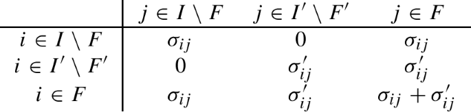
Here we can choose any subset $J_0$ of $I_0 \cup _\phi I'_0$ such that $\sigma _{ij}$ is integral unless $(i,j) \in J_0 \times J_0$. In this paper, we consider the minimal $J_0$ given by

$$\begin{aligned} J_0 = I_0 \cup _\phi I'_0 \setminus J_1, \quad J_1:= \{ i \in I_0 \cup _\phi I'_0 \mid \sigma _{ij} \in {\mathbb Z}\text { for all }j \in J \}. \end{aligned}$$

The amalgamation procedure can be upgraded to that for two seeds. Let $(Q,\textbf{X})$ and $(Q',\textbf{X}')$ be two seeds, $(F,F',\phi )$ a gluing data as above. Then we define a new seed $(Q *_\phi Q',\textbf{Y})$, where the weighted quiver $Q \cup _\phi Q'$ is given as above and the variables $\textbf{Y}=(Y_i)_{i \in J}$ is defined by

$$\begin{aligned} Y_i:= {\left\{ \begin{array}{ll} X_i &{} \text{ if } i \in I \setminus F \\ X'_i &{} \text{ if } i \in I' \setminus F' \\ X_i \cdot X'_{\phi (i)} &{} \text{ if } i \in F. \end{array}\right. } \end{aligned}$$

Then it is not hard to check that the amalgamation of seeds commutes with the mutation at any vertex $k \in (I {\setminus } I_0) \sqcup (I' {\setminus } I'_0)$. Thus for two seed patterns $\textsf{S}$ and $\textsf{S}'$ and a gluing data as above, we have a dominant morphism

$$\begin{aligned} \alpha _\phi : {\mathcal {X} }_{\textsf{S}} \times {\mathcal {X} }_{\textsf{S}'} \rightarrow {\mathcal {X} }_{\textsf{S}*_\phi \textsf{S}'}. \end{aligned}$$

Here the seed pattern $\textsf{S}*_\phi \textsf{S}'$ is obtained by the amalgamation of the seeds $\textsf{S}^{(t)}$ and ${\textsf{S}'}^{(t)}$ for $t \in \mathbb {T}_{I_\textrm{uf}}$.

1.3 B.3. Weighted quivers from reduced words

Let us fix a finite dimensional complex semisimple Lie algebra $\mathfrak {g}$. Let $C(\mathfrak {g})=(C_{st})_{s,t \in S}$ be the associated Cartan matrix. For $s \in S$, we define a weighted quiver $\textbf{J}^+(s)=(J(s),J_0(s),\sigma (s),d(s))$ as follows.

• $J(s)=J_0(s):=(S \setminus \{s\})\cup \{s^L,s^R\}$, where $s^L,s^R$ are new elements.

• The skew-symmetric matrix $\sigma (s)=(\sigma _{tu})_{t,u \in J(s)}$ is given by

  $$\begin{aligned}&\sigma _{s^R,s^L}=1, \\&\sigma _{s^L,u}=\sigma _{u,s^R}= {\left\{ \begin{array}{ll} 1/2 &{} \text {if }u \ne s\text { and }C_{su} \ne 0, \\ 0 &{} \text {if }u \ne s\text { and }C_{su}=0. \end{array}\right. } \end{aligned}$$

  Note that other entries are determined by the skew-symmetricity.

• d(s) is given by $d(s)_{s^{L,R}}:=d_s$, $d(s)_{t}:=d_t$ for $t \ne s$.

Let $\textbf{J}^-(s):=\textbf{J}^+(s)^{\textrm{op}}$. We call $\textbf{J}^\pm (s)$ the elementary quivers associated with $\mathfrak {g}$.

For each elementary quiver $\textbf{J}^\epsilon (s)$ with $s \in S$ and $\epsilon \in \{+,-\}$, we define a function $\delta (s): J(s) \rightarrow S$ on the set of vertices by $\delta (s)_{s^{L,R}}:=s$ and $\delta (s)_t:=t$ for $t \in S {\setminus } \{s^L,s^R\}$. We call $\delta$ the Dynkin labeling of vertices of $\textbf{J}^\epsilon (s)$.

Example B.4

Here are some examples of the elementary quivers.

• (1) Type $A_3$: $S=\{1,2,3\}$ and the Cartan matrix is given by

  $$\begin{aligned} C(A_3) = \begin{pmatrix} 2&{}\quad -1&{}\quad 0\\ -1&{}\quad 2&{}\quad -1\\ 0&{}\quad -1&{}\quad 2 \end{pmatrix}. \end{aligned}$$

  The elementary quivers $\textbf{J}^+(1)$, $\textbf{J}^+(2)$ and $\textbf{J}^+(3)$ are given as follows:

  

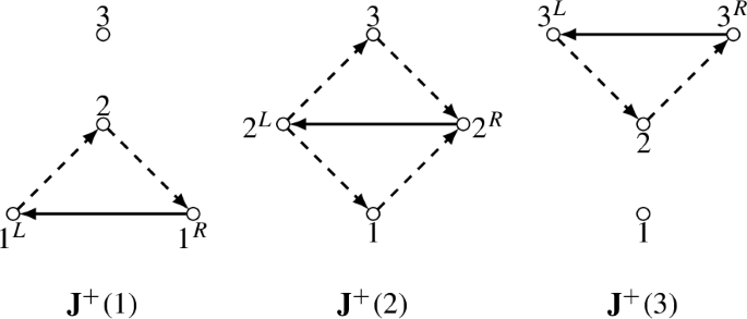
• (2) Type $C_3$: $S=\{1,2,3\}$ and the Cartan matrix is given by⁷

  $$\begin{aligned} C(C_3) = \begin{pmatrix} 2&{}\quad -1&{}\quad 0\\ -1&{}\quad 2&{}\quad -2\\ 0&{}\quad -1&{}\quad 2 \end{pmatrix}. \end{aligned}$$

  The elementary quivers $\textbf{J}^+(1)$, $\textbf{J}^+(2)$, $\textbf{J}^+(3)$ are given as follows.

  

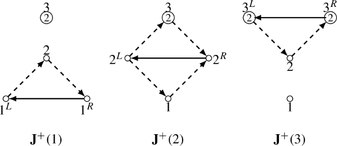
Note that the vertices with the same Dynkin label are drawn on the same level in the pictures.

For a reduced word ${\varvec{s}}=(s_1 \ldots s_l)$ of $u \in W(\mathfrak {g})$ and $\epsilon \in \{+,-\}$, we construct a weighted quiver $\textbf{J}^\epsilon ({\varvec{s}})=\textbf{J}^\epsilon (s_1,\ldots ,s_l)$ by amalgamating the elementary quivers $\textbf{J}^\epsilon (s_1),\cdots ,\textbf{J}^\epsilon (s_l)$ in the following way: for $k=1,\ldots ,l-1$, amalgamate $\textbf{J}^\epsilon (s_k)$ and $\textbf{J}^\epsilon (s_{k+1})$ by setting the gluing data in Definition B.3 as

$$\begin{aligned} F&:= J(s_k) \setminus \{s_k^L\}, \quad F':= J(s_{k+1}) \setminus \{s_{k+1}^R\}, \\ \phi&: F \rightarrow F',\quad s_k^R \mapsto s_k,~ s_{k+1} \mapsto s_{k+1}^L,~ t \mapsto t \text{ for } t \ne s_k,s_{k+1}. \end{aligned}$$

Note that the Dynkin labelings $\delta (s_k)$ are preserved under this amalgamation. Hence, these functions combine to give an S-valued function on the set of vertices of $J^\epsilon ({\varvec{s}})$, which we call the Dynkin labeling again. In the weighted quiver $\textbf{J}^+({\varvec{s}})=\textbf{J}^+(s_1)*\cdots *\textbf{J}^+(s_l)$, let $v_i^s$ be the $(i+1)$-st vertex with Dynkin label s from the left, for $s \in S$ and $i=0,\ldots ,n^s({\varvec{s}})$. Here $n^s({\varvec{s}})$ is the number of s which appear in the word ${\varvec{s}}$. We also use the labelling $v_i^s=: v_{k(s,i)}$ for $s \in S$ and $i=1,\ldots ,n^s({\varvec{s}})$, where $k(s,i) \in \{1,\ldots ,l\}$ denotes the i-th number k such that $s_k=s$ in the word ${\varvec{s}}$. Similarly, the vertices of $\textbf{J}^-({\varvec{s}}_{\textrm{op}}^*)$ are labeled as $\bar{v}_i^s=\bar{v}_{k(s,i)}$ where the index i runs from the left to the right.

Example B.5

Here are some examples of the weighted quiver $\textbf{J}^+({\varvec{s}})$ (left) and the corresponding quiver $\textbf{J}^-({\varvec{s}}_{\textrm{op}}^*)$ (right).

• (1) Type $A_3$, ${\varvec{s}}=(1,2,3,1,2,1)$ and ${\varvec{s}}_{\textrm{op}}^*=(3,2,3,1,2,3)$.

  

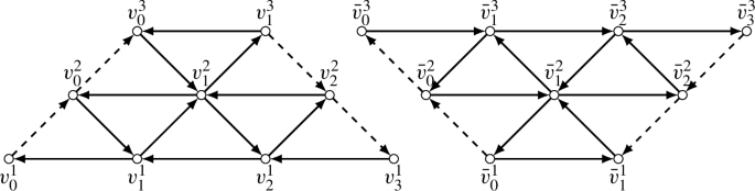
  Here the vertices $v_1^1$, $v_2^1$, $v_1^2$, $\bar{v}_1^3$, $\bar{v}_1^2$ and $\bar{v}_2^3$ are mutable.

• (2) Type $C_3$, ${\varvec{s}}=(1,2,3,1,2,3,1,2,3)$ and ${\varvec{s}}^*_\textrm{op}=(3,2,1,3,2,1,3,2,1)$.

  

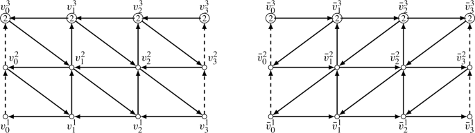
  Here the vertices $v_i^s$ and $\bar{v}_i^s$ for $s=1,2,3$, $i=1,2$ are mutable.

Note that the weighted quivers $\textbf{J}^+({\varvec{s}})$ and $\textbf{J}^-({\varvec{s}}_{\textrm{op}}^*)$ are isomorphic.

Next we recall the quiver $\widetilde{J}^+({\varvec{s}})$, which is called the decorated quiver in [23] in special cases. We follow a more general construction given in [18].

Let ${\varvec{s}}=(s_1,\ldots ,s_l)$ be a reduced word of $u \in W(\mathfrak {g})$. For $k=1,\ldots ,l$, let $\alpha ^{\varvec{s}}_k$ (resp. $\beta ^{\varvec{s}}_k$) be the root (resp. coroot) defined by

$$\begin{aligned} \alpha ^{\varvec{s}}_k:= r_{s_l}\ldots r_{s_{k+1}}\alpha _{s_k}, \quad \beta ^{\varvec{s}}_k:= r_{s_l}\ldots r_{s_{k+1}}\alpha ^\vee _{s_k}. \end{aligned}$$

Then for each $s \in S$, there exists a unique $k=k(s)$ such that $\beta ^{\varvec{s}}_k=\alpha ^\vee _s$. Note that from [27, (3.10.3)], we have $\alpha ^{\varvec{s}}_{k(s)}=\alpha _s$ at the same time. Let $\textbf{H}({\varvec{s}})=(H({\varvec{s}}),H_0({\varvec{s}}),{\varepsilon }({\varvec{s}}),d({\varvec{s}}))$ be the weighted quiver defined as follows.

• $H({\varvec{s}})=H_0({\varvec{s}}):=S$.

• The exchange matrix ${\varepsilon }({\varvec{s}})=({\varepsilon }_{st})_{s,t \in S}$ is given by

  $$\begin{aligned} {\varepsilon }_{st}:=\frac{\textrm{sgn}(k(t)-k(s))}{2}C_{st}. \end{aligned}$$

• $d({\varvec{s}})=(d({\varvec{s}})_s)_{s \in S}$ is given by $d({\varvec{s}})_s:=d_s$.

The vertex of $\textbf{H}({\varvec{s}})$ corresponding to $s \in S$ is denoted by $y_s$. Then we define $\widetilde{\textbf{J}}^+({\varvec{s}})$ to be the weighted quiver obtained from the disjoint union of the quivers $\textbf{J}^+({\varvec{s}})$ and $\textbf{H}({\varvec{s}})$ by adding the arrows $v_{k(s)-1} \rightarrow y_s$ and $y_s \rightarrow v_{k(s)}$ for each $s \in S$. As a convention, these additional arrows and the quiver $\textbf{H}({\varvec{s}})$ are shown in blue in figures.

Example B.6

Here are some examples of the quiver $\widetilde{\textbf{J}}^+({\varvec{s}})$.

• (1) Type $A_3$, ${\varvec{s}}=(1,2,3,1,2,1)$. The sequence $(\alpha _k^{\varvec{s}})_{k=1,\ldots ,6}$ is computed as

  $$\begin{aligned}&\alpha _6^{\varvec{s}}= \alpha _1, \quad \alpha _5^{\varvec{s}}=\alpha _1+\alpha _2, \quad \alpha _4^{\varvec{s}}=\alpha _2, \\&\alpha _3^{\varvec{s}}=\alpha _1+\alpha _2+\alpha _3, \quad \alpha _2^{\varvec{s}}=\alpha _2+\alpha _3, \quad \alpha _1^{\varvec{s}}=\alpha _3. \end{aligned}$$

  Thus we get $k(1)=6,~k(2)=4,~k(3)=1$, and the quiver $\widetilde{\textbf{J}}^+(1,2,3,1,2,1)$ is given by

  

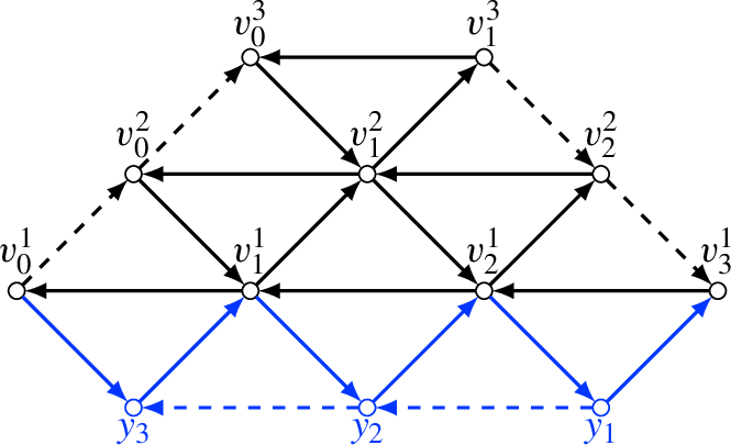
• (2) Type $C_3$, ${\varvec{s}}=(1,2,3,1,2,3,1,2,3)$. The sequence $(\alpha _k^{\varvec{s}})_{k=1,\ldots ,9}$ is computed as

  $$\begin{aligned}&\alpha _9^{\varvec{s}}= \alpha _3, \quad \alpha _8^{\varvec{s}}=\alpha _2+\alpha _3, \quad \alpha _7^{\varvec{s}}=\alpha _1+\alpha _2+\alpha _3, \\&\alpha _6^{\varvec{s}}= 2\alpha _2+\alpha _3, \quad \alpha _5^{\varvec{s}}=\alpha _1+2\alpha _2+\alpha _3, \quad \alpha _4^{\varvec{s}}=\alpha _2, \\&\alpha _3^{\varvec{s}}=2(\alpha _1+\alpha _2)+\alpha _3, \quad \alpha _2^{\varvec{s}}=\alpha _1+\alpha _2, \quad \alpha _1^{\varvec{s}}=\alpha _1. \end{aligned}$$

  Thus we get $k(1)=1,~k(2)=4,=k(3)=9$, and the quiver $\widetilde{\textbf{J}}^+((1,2,3)^3)$ is given by

  

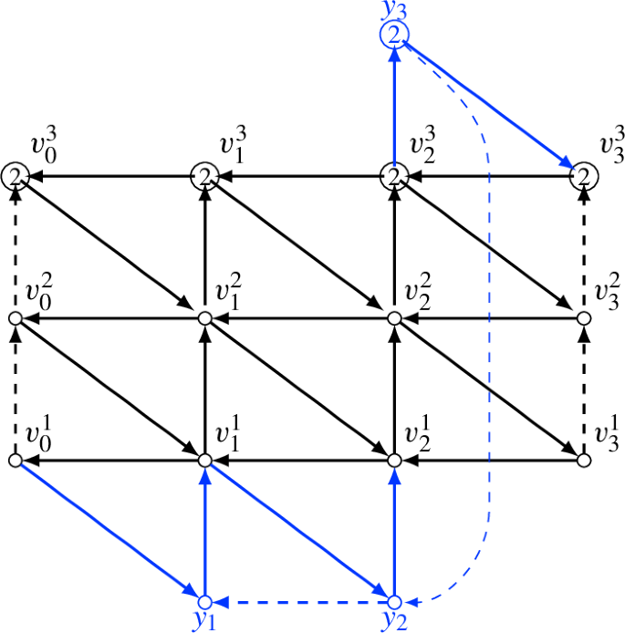
Appendix C. A short review on quotient stacks

We shortly recall some basic facts on the quotient stacks, to the minimal extent we need to recognize the moduli spaces ${\mathcal {P} }_{G,\Sigma }$ correctly. We refer the reader to [17, 41] for a self-contained presentation of the general theory of (algebraic) stacks. The lecture note [22] will be also useful to get an intuition for stacks for the readers more familiar with the differential geometry or the algebraic topology than the algebraic geometry.

Let X be an algebraic variety (or more generally, a scheme), and G an affine algebraic group acting on X algebraically. In order to study the quotient of X by G from the viewpoint of algebraic geometry, a good way is to define it as a quotient stack [X/G]. Morally, the geometry of [X/G] is the G-equivariant geometry of X. Several lemmas below will justify this slogan. When the action of G is free, one can think of [X/G] as an algebraic variety (Lemma C.5); in general, the quotient stack [X/G] also contains the information on the stabilizers.

Let X be a scheme over ${\mathbb C}$ and G an affine algebraic group acting on X. Then the quotient stack ${\mathcal {X} }=[X/G]$ is a category fibered in groupoids ( [17, Definition 2.15]) where the objects over a scheme B are pairs (E, f) of a principal G-bundle $E \rightarrow B$ and a G-equivariant morphism $f:E \rightarrow X$; morphisms over B are Cartesian diagrams of G-bundles which respect the equivariant morphisms to X.

Note that an object (E, f) over $B={{\,\mathrm{\textrm{Spec}}\,}}{\mathbb C}$ can be viewed as a G-orbit in X. Thus the set X/G of orbits is recovered as the set of images of $f:E \rightarrow X$, that is, the isomorphism classes of the objects of ${\mathcal {X} }({{\,\mathrm{\textrm{Spec}}\,}}{\mathbb C})$. Yoneda’s lemma for stacks implies that a morphism $u: B \rightarrow {\mathcal {X} }$ from a scheme B corresponds to an object of ${\mathcal {X} }(B)$.

It is known that ${\mathcal {X} }$ is an Artin stack ( [17, Definition 2.26]): an atlas is defined by the morphism $X \rightarrow {\mathcal {X} }$ given by the pull-back of the trivial bundle $X \times G$ (see [17, Example 2.29]). The structure sheaf on ${\mathcal {X} }$ and the ${\mathbb C}$-algebra $\mathcal {O}({\mathcal {X} })$ of global functions (function algebra) are defined, for example as in [22, Section 4]. One can verify the following:

Lemma C.1

$\mathcal {O}({\mathcal {X} }) \cong \mathcal {O}(X)^G$.

A scheme V can be regarded as an Artin stack whose objects over B are morphisms $B \rightarrow V$; the only morphism over B is the identity. A stack is said to be representable if it is isomorphic to a stack arising from a scheme. For two Artin stacks ${\mathcal {X} }$ and $\mathcal {Y}$, a morphism $\phi : {\mathcal {X} }\rightarrow \mathcal {Y}$ of stacks is said to be representable if for any morphism $B \rightarrow \mathcal {Y}$, the fiber product $B \times _{\mathcal {Y}} {\mathcal {X} }$ is representable. Informally speaking, a morphism $B \rightarrow \mathcal {Y}$ can be viewed as a “local chart” on $\mathcal {Y}$, and the induced morphism $B \times _{\mathcal {Y}} {\mathcal {X} }\rightarrow B$ is the “local expression” of $\phi$. Here is an easy example:

Lemma C.2

Let V be a scheme over ${\mathbb C}$ and G an affine algebraic group. Consider the G-action on $V \times G$ given by the trivial action on the first factor and left multiplication on the second. Then the quotient stack $[V \times G/G]$ is representable by V.

The following lemma tells us that we can obtain morphisms between quotient stacks from equivariant morphisms of varieties.

Lemma C.3

Let ${\mathcal {X} }=[X/H]$ and $\mathcal {Y}=[Y/G]$ be two quotient stacks. Let $\phi :X \rightarrow Y$ be a morphism equivariant with respect to an embedding $\tau :H \rightarrow G$. Then it induces a representable morphism $\phi _*: {\mathcal {X} }\rightarrow \mathcal {Y}$ of Artin stacks. More precisely, for any morphism $u: B \rightarrow \mathcal {Y}$ from a scheme B which corresponds to an object $(E,f) \in \mathcal {Y}(B)$, the diagram

is Cartesian. Here $u_H$ is a morphism corresponding to an H-bundle $E \rightarrow E \times (G/H) \rightarrow E \times _G (G/H)$.

We give a proof for our convenience.

Proof

For an object (E, f) over B in ${\mathcal {X} }$, the pair $\phi _*(E,f):=(E,\phi \circ f)$ is an object over B in $\mathcal {Y}$. This correspondence is clearly compatible with pull-backs, and defines a morphism $\phi _*: {\mathcal {X} }\rightarrow \mathcal {Y}$. It is not hard to see that the fiber product $B \times _{\mathcal {Y}}{\mathcal {X} }$ is isomorphic to $E\times _G (G/H)$, with a notice that an H-sub-bundle of a G-bundle $P \rightarrow B$ is in one-to-one correspondence with a section of the associated bundle $P \times _G (G/H)$. Thus $\phi _*$ it is representable. $\square$

We call $\phi$ a presentation of the morphism $\phi _*$.

Remark C.4

When $\tau$ is not an embedding, the morphism $\phi _*$ is not representable in general. For instance, the morphism $(\textrm{id}_{pt})_*: [pt/G] \rightarrow [pt/e] = pt$ is not representable for a non-trivial group G, where pt denotes the point scheme and e is the trivial group.

A property of morphisms of schemes that are local in nature on the target and stable under base-change can be defined for representable morphisms of stacks. For instance, $\phi _*$ is said to be an open embedding if $\phi :X=Y \times _{[Y/G]} [X/G] \rightarrow Y$ is an open embedding of varieties.

Lemma C.5

Suppose that X is an affine algebraic variety, G is reductive, and the G-action on X is free. Then the quotient stack ${\mathcal {X} }=[X/G]$ is representable by the geometric quotient X/G.

Indeed, the assumptions imply that all points of X are G-stable, and the geometric quotient X/G exists (see, for instance, [3, Proposition 1.26]).

References

Berenstein, A., Zelevinsky, A.: Total positivity in Schubert varieties. Comment. Math. Helv. 72(1), 128–166 (1997)
Berenstein, A., Fomin, S., Zelevinsky, A.: Parametrizations of canonical bases and totally positive matrices. Adv. Math. 122(1), 49–149 (1996)
Brion, M.: Introduction to actions of algebraic groups, http://www-fourier.ujf-grenoble.fr/~mbrion/notes_luminy.pdf
Chekhov, L.O., Shapiro, M.: Darboux coordinates for symplectic groupoid and cluster algebras, arXiv:2003.07499
Douglas, D.: Points of quantum \(SL_n\) coming from quantum snakes, arXiv:2103.04471
Fock, V. V., Goncharov, A. B.: Cluster \({\cal{X}}\)-varieties, amalgamation and Poisson-Lie groups, Algebraic geometry and number theory, volume 253 of Progr. Math., PP 27–68, Birkhäuser Boston, Boston, MA, (2006)
Fock, V. V., Goncharov, A. B.: Dual Teichmüller and lamination spaces, Handbook of Teichmüller theory, Vol. I, 647-684; IRMA Lect. Math. Theor. Phys., 11, Eur. Math. Soc., Zürich, (2007)
Fock, V. V.: Description of moduli space of projective structures via fat graphs, arXiv:hep-th/9312193
Fock, V.V., Goncharov, A.B.: Moduli spaces of local systems and higher Teichmüller theory. Publ. Math. Inst. Hautes Études Sci. 103, 1–211 (2006)
Fock, V.V., Goncharov, A.B.: The quantum dilogarithm and representations of quantum cluster varieties. Invent. Math. 175(2), 223–286 (2009)
Fock, V.V., Goncharov, A.B.: Cluster ensembles, quantization and the dilogarithm. Ann. Sci. Éc. Norm. Supér. 42(6), 865–930 (2009)
Fomin, S., Shapiro, M., Thurston, D.: Cluster algebras and triangulated surfaces. I. Cluster complexes. Acta Math. 201(1), 83–146 (2008)
Gaiotto, D., Moore, G.W., Neitzke, A.: Spectral networks and snakes. Ann. Henri Poincaré 15(1), 61–141 (2014)
Geiß, C., Leclerc, B., Schröer, J.: Kac-Moody groups and cluster algebras. Adv. Math. 228(1), 329–433 (2011)
Geiß, C., Leclerc, B., Schröer, J.: Generic bases for cluster algebras and the Chamber ansatz. J. Amer. Math. Soc. 25(1), 21–76 (2012)
Goldman, W.M.: Invariant functions on Lie groups and Hamiltonian flows of surface group representations. Invent. Math. 85(2), 263–302 (1986)
Gómez, T.L.: Algebraic stacks. Proc. Indian Acad. Sci. Math. Sci. 111(1), 1–31 (2001)
Goncharov, A. B., Shen, L.: Quantum geometry of moduli spaces of local systems and representation theory, arXiv:1904.10491v2
Goncharov, A.B., Shen, L.: Geometry of canonical bases and mirror symmetry. Invent. Math. 202(2), 487–633 (2015)
Goncharov, A.B., Shen, L.: Donaldson-Thomas transformations of moduli spaces of \(G\)-local systems. Adv. Math. 327, 225–348 (2018)
Gross, M., Hacking, P., Keel, S., Kontsevich, M.: Canonical bases for cluster algebras. J. Amer. Math. Soc. 31(2), 497–608 (2018)
Heinloth, J.: Notes on differentiable stacks, Mathematisches Institut, Georg-August-Universität Göttingen: Seminars Winter Term 2004/2005, 1–32, Universitätsdrucke Göttingen, Göttingen (2005)
Inoue, R., Ishibashi, T., Oya, H.: Cluster realizations of Weyl groups and higher Teichmüller theory. Sel. Math. New Ser. 27, 37 (2021)
Ishibashi, T., Oya, H., Shen, L.: \({{\mathscr {A}}}={{\mathscr {U}}}\) for cluster algebras from moduli spaces of \(G\)-local systems. Adv. Math. 431, 109256 (2023)
Jantzen, J.C.: Representations of algebraic groups, Second edition. Mathematical Surveys and Monographs, 107. American Mathematical Society, Providence, RI, (2003). xiv+576 pp
Jordan, D., Le, I., Schrader, G., Shapiro, A.: Quantum decorated character stacks, arXiv:2102.12283
Kac, V.: Infinite-dimensional Lie algebras. Third edition, Cambridge University Press, Cambridge, (1990). xxii+400 pp
Kang, S.-J., Kashiwara, M.: Categorification of highest weight modules via Khovanov-Lauda-Rouquier algebras. Invent. Math. 190(3), 699–742 (2012)
Kang, S.-J., Kashiwara, M., Kim, M., Oh, S.-J.: Monoidal categorification of cluster algebras. J. Amer. Math. Soc. 31(2), 349–426 (2018)
Kashiwara, M., Kim, M., Oh, S.-J., Park, E.: Monoidal categories associated with strata of flag manifolds. Adv. Math. 328, 959–1009 (2018)
Kashiwara, M., Kim, M., Oh, S.-J., Park, E.: Localizations for quiver Hecke algebras. Pure Appl. Math. Q. 17(4), 1465–1548 (2021)
Khovanov, M., Lauda, A.: A diagrammatic approach to categorification of quantum groups. I. Represent. Theo. 13, 309–347 (2009)
Khovanov, M., Lauda, A.: A diagrammatic approach to categorification of quantum groups II. Trans. Amer. Math. Soc. 363(5), 2685–2700 (2011)
Kimura, Y., Oya, H.: Twist automorphisms on quantum unipotent cells and dual canonical bases. Int. Math. Res. Not. IMRN 9, 6772–6847 (2021)
Le, I.: Cluster structure on higher Teichmüller spaces for classical groups. Forum Math. Sigma 7, e13,165 (2019)
Penner, R.C.: Decorated Teichmüller theory, QGM Master Class Series, European Mathematical Society (EMS), Zürich (2012)
Rouquier, R.: \(2\)-Kac-Moody algebras, arXiv:0812.5023v1
Rouquier, R.: Quiver Hecke algebras and \(2\)-Lie algebras. Algebra Colloq. 19(2), 359–410 (2012)
Schrader, G., Shapiro, A.: Continuous tensor categories from quantum groups I: algebraic aspects, arXiv:1708.08107
Shen, L.: Duals of semisimple Poisson-Lie groups and cluster theory of moduli spaces of \(G\)-local systems. Int. Math. Res. Not. IMRN 18, 14295–14318 (2022)
The Stacks Project Authors, Stacks project, https://stacks.math.columbia.edu
Williams, H.: Cluster ensembles and Kac-Moody groups. Adv. Math. 247, 1–40 (2013)
Acknowledgements
The authors’ deep gratitude goes to Linhui Shen for his insightful comments on this paper at several stages and explaining his works with Alexander Goncharov. They are grateful to Tatsuki Kuwagaki and Takuma Hayashi for explaining some basic notions and backgrounds on Artin stacks, and giving valuable comments on a draft of this paper. They also wish to thank Ryo Fujita for helpful discussions on quiver Hecke algebras. The authors are grateful to the anonymous referee for the careful reading of the paper and the significant comments. T. I. would like to express his gratitude to his former supervisor Nariya Kawazumi for his continuous guidance and encouragement in the earlier stage of this work. T. I. is partially supported by JSPS KAKENHI Grant Numbers 18J13304 and 20K22304, and the Program for Leading Graduate Schools, MEXT, Japan. H. O. is supported by JSPS Grant-in-Aid for Early-Career Scientists (No. 19K14515).
Author information
Authors and Affiliations
Corresponding author
Additional information
Publisher's Note
Springer Nature remains neutral with regard to jurisdictional claims in published maps and institutional affiliations.