Magnitude cohomology

Abstract

Magnitude homology was introduced by Hepworth and Willerton in the case of graphs, and was later extended by Leinster and Shulman to metric spaces and enriched categories. Here we introduce the dual theory, magnitude cohomology, which we equip with the structure of an associative unital graded ring. Our first main result is a ‘recovery theorem’ showing that the magnitude cohomology ring of a finite metric space completely determines the space itself. The magnitude cohomology ring is non-commutative in general, for example when applied to finite metric spaces, but in some settings it is commutative, for example when applied to ordinary categories. Our second main result explains this situation by proving that the magnitude cohomology ring of an enriched category is graded-commutative whenever the enriching category is cartesian. We end the paper by giving complete computations of magnitude cohomology rings for several large classes of graphs.

1 Introduction

1.1 Overview

In this paper we introduce and investigate magnitude cohomology of generalised metric spaces and enriched categories. Our theory is dual, in the same sense as singular homology and cohomology, to the theory of magnitude homology introduced by Hepworth and Willerton [7] and later extended by Leinster and Shulman [13]. As in the singular case, we find that the introduction of cohomology adds strength and structure to the whole theory. We show that the magnitude cohomology groups form a unital associative graded ring, which is noncommutative in many cases. We prove a recovery theorem which shows that the magnitude cohomology of a large class of metric spaces (including finite metric spaces and arbitrary directed graphs) completely determines the metric space in question. Moving to the context of enriched categories, we prove that the magnitude cohomology ring of an enriched category is graded-commutative so long as the enriching category is cartesian. Finally, specialising to undirected graphs, we give complete computations of the magnitude cohomology ring for diagonal graphs and for odd cyclic graphs, and we establish a connection between magnitude cohomology and the quiver algebra of a graph.

1.2 Background and motivation

Leinster’s theory of magnitude is a mechanism that associates numerical invariants to mathematical objects of various kinds. In greatest generality it is an invariant of enriched categories. The power of this theory is that different choices of enriching category take us into different regions of mathematics, with notions of magnitude for posets, categories, graphs, metric spaces and more, and that the resulting invariants are meaningful and interesting in many of these settings. In the case of finite posets the magnitude is precisely the Euler characteristic of the order complex. For finite categories the magnitude encompasses the Euler characteristic of the classifying space and the cardinality of groupoids, but is defined more generally. In the case of graphs the magnitude is a formal power series with many attractive properties, such as product and inclusion–exclusion formulas, and invariance under certain Whitney twists. The magnitude of finite metric spaces is a cardinality-like invariant, described as the ‘effective number of points’, that first arose as a measurement of biological diversity [15]. Perhaps more importantly, the magnitude of finite metric spaces can be extended to compact metric spaces. In this setting the magnitude is known to encode geometric information, such as the volume and perimeter of domains in odd-dimensional Euclidean space [4], although it remains rather mysterious and difficult to compute. We refer the reader to [10] for magnitude of ordinary categories and posets, [11] for enriched categories and metric spaces, and [12] for graphs.

Magnitude homology was first introduced by the author and Willerton [7] in the setting of graphs, and it categorifies the magnitude in exactly the same sense that Khovanov homology categorifies the Jones polynomial. Leinster and Shulman later extended magnitude homology to categories enriched in a semicartesian category [13], they showed that it determines the magnitude in favourable circumstances, and they specialised the definition to obtain the magnitude homology of metric spaces. Magnitude homology has shown itself to be an important extension and refinement of magnitude, with many characteristic features of homology theories and categorification:

• Magnitude homology of graphs has properties (such as Künneth and Mayer–Vietoris theorems) that categorify and explain properties of magnitude (such as the product rule and inclusion–exclusion formula) [7].

• The phenomenon of alternating coefficients in the magnitude of certain graphs was explained by the notion of diagonal graphs in [7, Section 7].

• Graphs (and therefore metric spaces) with the same magnitude can have distinct magnitude homology groups. The first known example of such a pair is the $4\times 4$ rook’s graph and the Shrikhande graph, and is due to Yuzhou Gu. See Appendix A of Gu’s paper [5] and also the comments at the blogpost [17].

• Magnitude homology of graphs (and therefore metric spaces) can contain torsion, and in particular magnitude homology is not determined by its ranks. The first example of this was obtained by Kaneta and Yoshinaga in [9, Corollary 5.12].

• A metric space X is Menger convex if and only if its magnitude homology groups vanish in (homological) degree 1 [13, Corollary 4.5].

We would also like to mention recent work of Otter [14], which establishes a connection between magnitude homology and topology. Otter introduces blurred magnitude homology of metric spaces, a persistent version of the theory, and shows that a certain inverse limit of the blurred magnitude homology produces the Vietoris homology. The latter is a homology theory for metric spaces that coincides with singular homology in certain cases, for example for compact Riemannian manifolds.

1.3 Metric spaces

Our first results are in the setting of generalised metric spaces [18, 19]. We introduce the magnitude cohomology of a generalised metric space X, which is a bigraded abelian group $\mathrm {MH}^*_*(X)$ consisting of groups $\mathrm {MH}_\ell ^k(X)$ where $k=0,1,2,\ldots$ and $\ell \in [0,\infty )$. It is equipped with a product operation

$$\begin{aligned} \mathrm {MH}^j_\ell (X)\otimes \mathrm {MH}^k_m(X) \longrightarrow \mathrm {MH}^{j+k}_{\ell +m}(X) \end{aligned}$$

that gives it the structure of an associative unital ring. This ring structure is in general noncommutative, as we show in Proposition 2.3. In Theorem 3.1 we give a ‘recovery theorem’ which shows that for a large class of metric spaces X, including all graphs and finite metric spaces, the magnitude cohomology ring $\mathrm {MH}^*_*(X)$ is sufficient to determine X precisely. This is in stark contrast to the situation for magnitude homology, or for magnitude cohomology without the ring structure, where for example any two trees with the same number of vertices have isomorphic magnitude homology.

1.4 Enriched categories

The next part of the paper deals with magnitude cohomology of enriched categories. For this we fix a symmetric monoidal semicartesian category $\mathcal {V}$ and a strong monoidal functor $\Sigma :\mathcal {V}\rightarrow \mathcal {A}$ into a closed symmetric monoidal abelian category $\mathcal {A}$. In this situation Leinster and Shulman defined the magnitude homology $H^\Sigma _*(X)$ of a $\mathcal {V}$-category X [13]. We define the dual theory, the magnitude cohomology $H^*_\Sigma (X)$ of a $\mathcal {V}$-category X, and we equip it with a product

$$\begin{aligned} H^j_\Sigma (X)\otimes H^k_\Sigma (X)\longrightarrow H^{j+k}_\Sigma (X) \end{aligned}$$

and unit $1_\mathcal {A}\rightarrow H^0_\Sigma (X)$ that make it into an associative unital graded ring in $\mathcal {A}$. By choosing appropriate $\mathcal {V}$, $\mathcal {A}$ and $\Sigma$, we obtain magnitude cohomology rings for posets, small categories, and generalised metric spaces, and we show that these respectively recover the cohomology of the order complex with the cup product, the cohomology of the classifying space with the cup product, and the magnitude cohomology ring respectively. Note that in the first two cases the product is graded-commutative, but in the third case it is not. In Theorem 5.7 we explain this phenomenon by showing that in general, when the enriching category $\mathcal {V}$ is cartesian, the magnitude cohomology ring is graded-commutative. The enriching categories for posets and small categories are cartesian, while the enriching category for generalised metric spaces is not.

1.5 Graphs

Finally we specialise to finite graphs, and we give complete computations of the magnitude cohomology ring for several classes of graphs. The magnitude cohomology rings in question are all highly nontrivial, but nevertheless they all admit nice presentations.

In Theorem 6.2 we identify the diagonal part of the magnitude cohomology ring, given by the groups $\mathrm {MH}^k_k(G)$, as a quotient of the path algebra of the quiver obtained from G by doubling the edges. In [7, Section 7] we introduced diagonal graphs, which are graphs whose magnitude homology (and therefore cohomology) is concentrated on this diagonal, and we identified various large classes of diagonal graphs. Work of Gu [5] has added to the known examples. Theorem 6.2 therefore gives a complete description of the magnitude cohomology ring of any diagonal graph, and we make this description explicit in the case of trees, complete graphs, and complete bipartite graphs.

In Theorem 7.1 we give an explicit presentation of the magnitude cohomology rings of the odd cyclic graphs (which are not diagonal). This is based on Gu’s computation of the magnitude homology of odd cyclic graphs given in Theorem 4.6 of [5].

1.6 Organisation of the paper

The paper is organised as follows. In Sect. 2 we define the magnitude cohomology of metric spaces, together with its ring structure, and we relate it to magnitude. In Sect. 3 we state and prove our recovery theorem. In Sect. 4 we give a brief exposition of Leinster and Shulman’s theory of magnitude homology of enriched categories. Then in Sect. 5 we define magnitude cohomology of enriched categories, we define its ring structure, and we prove that it is commutative when the enriching category is cartesian. In Sect. 6 we explore the case of finite graphs, we express the diagonal part of magnitude cohomology as a quotient of the path algebra of the associated quiver, and we compute the magnitude cohomology ring for several classes of diagonal graphs. In Sect. 7 we compute the magnitude cohomology ring of odd cyclic graphs.

1.7 Acknowledgements

Thanks to Simon Willerton for some useful comments, and to Tom Leinster for explaining the connection between dagger categories and symmetry in generalised metric spaces.

2 Magnitude cohomology of metric spaces

In this section we recall the magnitude homology of generalised metric spaces, and we then define their magnitude cohomology and equip it with the structure of a graded associative unital ring. We show that this ring is typically not graded commutative, and we show how to recover the magnitude from the magnitude cohomology.

We work with generalised metric spaces in the sense of Lawvere [18, 19]. Recall that a generalised metric space, or extended pseudo-quasi-metric space, is defined in the same way as a metric space, except that the metric takes values in $[0,\infty ]$ (extended), distances between distinct points may be 0 (pseudo), and the distance from a to b need not equal the distance from b to a (quasi). Generalised metric spaces are the same thing as categories enriched in $[0,\infty ]$. The objects of the enriched category correspond to the points of the space, and the morphism object $X(a,b)\in [0,\infty ]$ corresponds to the distance from a to b. We will work with generalised metric spaces where possible, restricting to extended quasi-metric spaces where necessary.

Definition 2.1

(Magnitude homology) We recall the definition of magnitude homology from sections 2 and 3 of [7] (for graphs) and section 3 of [13] (for arbitrary metric spaces).

Let X be a generalised metric space. A k-simplex or just simplex in X is a tuple $(x_0,\ldots ,x_k)$ of elements of X in which consecutive entries are distinct, i.e. $x_0\ne x_1\ne \cdots \ne x_k$. The degree of the simplex $(x_0,\ldots ,x_k)$ is k, and its length is

$$\begin{aligned} \ell (x_0,\ldots ,x_k) =d(x_0,x_1)+\cdots +d(x_{k-1},x_k). \end{aligned}$$

The magnitude chain complex of X, denoted $\mathrm {MC}_{*,*}(X)$, is the chain complex of $\mathbb {R}$-graded abelian groups defined as follows. The k-chains in degree $\ell$, denoted $\mathrm {MC}_{k,\ell }(X)$, is defined to be the free abelian group on the simplices of degree k and length $\ell$:

$$\begin{aligned} \mathrm {MC}_{k,\ell }(X) = \mathbb {Z}\left\{ (x_0,\ldots ,x_k)\in X^{k+1} \mid \ell (x_0,\ldots ,x_k)=\ell ,\ x_0\ne x_1\ne \cdots \ne x_k \right\} \end{aligned}$$

The differential

$$\begin{aligned} \partial :\mathrm {MC}_{k,l}(X)\longrightarrow \mathrm {MC}_{k-1,l}(X) \end{aligned}$$

is defined by

$$\begin{aligned} \partial =-\partial _1+\partial _2-\cdots +(-1)^{k-1}\partial _{k-1} \end{aligned}$$

where

$$\begin{aligned} \partial _i(x_0,\ldots ,x_k)= \left\{ \begin{array}{ll} (x_0,\ldots ,\widehat{x_i},\ldots ,x_k) &{} \text {if }d(x_{i-1},x_{i+1})=d(x_{i-1},x_i)+d(x_i,x_{i+1}), \\ 0 &{} \text {otherwise}. \end{array} \right. \end{aligned}$$

The magnitude homology $\mathrm {MH}_{*,*}(X)$ of X is the homology of the magnitude chain complex:

$$\begin{aligned} \mathrm {MH}_{*,\ell }(X)=H_*(\mathrm {MC}_{*,\ell }(X)). \end{aligned}$$

Note that in [13] $\mathrm {MH}_{k,\ell }(X)$ is denoted by $H_{k,\ell }(X)$. If $f:X\rightarrow Y$ is a map of generalised metric spaces that does not increase distances, i.e. $d_Y(f(x),f(x'))\leqslant d_X(x,x')$ for all $x,x'\in X$, then the induced chain map

$$\begin{aligned} f_\#:\mathrm {MC}_{*,*}(X)\rightarrow \mathrm {MC}_{*,*}(Y)\end{aligned}$$

is defined by

$$\begin{aligned} f_\#(x_0,\ldots ,x_k) = \left\{ \begin{array}{ll} (f(x_0),\ldots ,f(x_k)) &{} \text {if }\ell (f(x_0),\ldots ,f(x_k))=\ell (x_0,\ldots ,x_k) \\ 0 &{} \text {otherwise}. \end{array}\right. \end{aligned}$$

The induced map in homology is the map

$$\begin{aligned} f_*:\mathrm {MH}_{*,*}(X)\longrightarrow \mathrm {MH}_{*,*}(Y) \end{aligned}$$

obtained from $f_\#$.

We now define magnitude cohomology by dualising the above definition and equipping it with a product structure.

Definition 2.2

(Magnitude cohomology) Let X be a generalised metric space. The magnitude cochain complex of X is the dual to the magnitude chain complex:

$$\begin{aligned} \mathrm {MC}_\ell ^*(X)={{\,\mathrm{Hom}\,}}(\mathrm {MC}_{*,\ell }(X),\mathbb {Z}). \end{aligned}$$

The magnitude cohomology of X, denoted $\mathrm {MH}_*^*(X)$, is the cohomology of the magnitude cochains:

$$\begin{aligned} \mathrm {MH}_\ell ^*(X) = H^*(\mathrm {MC}_\ell ^*(X)). \end{aligned}$$

If $f:X\rightarrow Y$ is a non-increasing map of generalised metric spaces, then the dual of $f_\#$ gives the induced cochain map

$$\begin{aligned}f^\#:\mathrm {MC}_*^*(X)\longrightarrow \mathrm {MC}_*^*(Y)\end{aligned}$$

and the induced map in cohomology

$$\begin{aligned}f^*:\mathrm {MH}_*^*(X)\longrightarrow \mathrm {MH}_*^*(Y).\end{aligned}$$

Given $\varphi \in \mathrm {MC}^{k_1}_{\ell _1}(X)$ and $\psi \in \mathrm {MC}^{k_2}_{\ell _2}(X)$, the product $\varphi \cdot \psi \in \mathrm {MC}^{k_1+k_2}_{\ell _1+\ell _2}(X)$ is defined on $(x_0,\ldots ,x_{k_1+k_2})\in \mathrm {MC}_{k_1+k_2,\ell _1+\ell _2}(X)$ by

$$\begin{aligned} (\varphi \cdot \psi ) (x_0,\ldots ,x_{k_1+k_2}) = \varphi (x_0,\ldots ,x_{k_1})\cdot \psi (x_{k_1},\ldots ,x_{k_1+k_2}) \end{aligned}$$

if the lengths are compatible in the sense that $\ell (x_0,\ldots ,x_{k_1})=\ell _1$ and $\ell (x_{k_1},\ldots ,x_{k_1+k_2})=\ell _2$, and by

$$\begin{aligned} (\varphi \cdot \psi ) (x_0,\ldots ,x_{k_1+k_2}) = 0 \end{aligned}$$

otherwise. The unit $u\in \mathrm {MC}^0_0(X)$ is the cochain defined by the rule

$$\begin{aligned} u(x_0) = 1 \end{aligned}$$

for every 0-simplex $(x_0)$. The reader may readily verify that the product is strictly associative and unital, with unit u, and that it satisfies the Leibniz rule

$$\begin{aligned} \partial ^*(\varphi \cdot \psi ) =\partial ^*\varphi \cdot \psi + (-1)^{k_1}\varphi \cdot \partial ^*\psi . \end{aligned}$$

Consequently, there is an induced product on magnitude cohomology

$$\begin{aligned} \mathrm {MH}_{\ell _1}^{k_1}(X)\otimes \mathrm {MH}_{\ell _2}^{k_2}(X) \longrightarrow \mathrm {MH}_{\ell _1+\ell _2}^{k_1+k_2}(X), \quad \alpha \otimes \beta \longmapsto \alpha \cdot \beta \end{aligned}$$

that makes $\mathrm {MH}^*_*(X)$ into a unital, associative bigraded ring with unit $1=[u]\in \mathrm {MH}^0_0(X)$. We refer to $\mathrm {MH}^*_*(X)$, equipped with the product, as the magnitude cohomology ring. The assignment $X\mapsto \mathrm {MH}^*_*(X)$, $f\mapsto f^*$ is a contravariant functor from the category of metric spaces and non-increasing maps into the category of unital associative bigraded rings.

Our definition of the product on magnitude cohomology is similar to the definition of the cup-product in singular cohomology. Compare Definition 2.2 with Section 3.2 of [6], say. But in fact we know of no direct relationship between the two, and moreover we will see an important difference in the next proposition.

Recall from [13] that elements x, y in a generalised metric space are adjacent if d(x, y) is nonzero and finite and $d(x,y) = d(x,a) + d(a,y)\implies a=x\text { or }a=y$. Observe that any graph with at least one edge, and any finite metric space with at least two points, contains at least one adjacent pair.

Proposition 2.3

Suppose that X is an extended quasi-metric space containing an adjacent pair (x, y). Then $\mathrm {MH}^*_*(X)$ is not graded-commutative.

Proof

The proof of [13, Theorem 4.3] (compare with [7, Proposition 2.9]) can be dualised to show that if (x, y) is an adjacent pair in X, then there is a cocycle $\varphi _{xy}\in \mathrm {MC}^1_{d(x,y)}(X)$ defined by

$$\begin{aligned} \varphi _{xy}(x',y') = \left\{ \begin{array}{ll} 1 &{} \text {if }(x',y')=(x,y), \\ 0 &{} \text {otherwise}, \end{array}\right. \end{aligned}$$

and that the cohomology classes $a_{xy}=[\varphi _{xy}]$ for (x, y) adjacent form a basis of $\mathrm {MH}^1_*(X)$. Note that the proof of Theorem 4.3 of [13] is stated only for metric spaces, but that the proof extends to the extended quasi-metric case without change. Given such an adjacent pair (x, y), one may check that $(x,y,x)\in \mathrm {MC}_{2,d(x,y)+d(y,x)}(X)$ is a cycle, and that

$$\begin{aligned} \langle a_{xy}\cdot a_{yx},[(x,y,x)]\rangle = 1, \qquad \langle a_{yx}\cdot a_{xy},[(x,y,x)]\rangle = 0, \end{aligned}$$

so that $a_{xy}\cdot a_{yx}$ and $a_{yx}\cdot a_{xy}$ are not equal up to any choice of sign. Here $\langle -,-\rangle$ denotes the Kronecker pairing between homology and cohomology; see Remark 2.5 below. $\square$

Just as magnitude homology is a categorification of the magnitude of graphs and metric spaces (see [7,  Theorem 2.8] and [13,  Theorem 3.5]), the same is true of magnitude cohomology. To see this, we use the version of the magnitude from [13] that takes values in the field of Novikov series. For details on this we refer the reader to [13], in particular Definition 3.1, Theorem 3.2, and the discussion that precedes them.

Theorem 2.4

Let X be a finite quasi-metric space. Then

$$\begin{aligned} \# X = \sum _{\ell \geqslant 0}\sum _{k=0}^\infty (-1)^k \cdot {{\,\mathrm{rank}\,}}(\mathrm {MH}_{\ell }^k(X)) \cdot q^\ell , \end{aligned}$$

where each sum over k is finite, and the infinite sum over $\ell$ converges in the topology of .

Proof

Theorem 3.5 of [13] gives the same result but with ${{\,\mathrm{rank}\,}}(\mathrm {MH}_{k,\ell }(X))$ in place of ${{\,\mathrm{rank}\,}}(\mathrm {MH}^k_\ell (X))$. That the two ranks are equal follows from the universal coefficient sequence of Remark 2.5 below, together with the fact that $\mathrm {Ext}(\mathrm {MH}_{k,\ell }(X),\mathbb {Z})$ is finite since $\mathrm {MH}_{k,\ell }(X)$ is finitely generated. $\square$

We end this section with some remarks.

Remark 2.5

(The universal coefficient sequence) Magnitude homology and cohomology are related by a universal coefficient sequence:

$$\begin{aligned} 0\rightarrow \mathrm {Ext}(\mathrm {MH}_{k-1,\ell }(X),\mathbb {Z}) \longrightarrow \mathrm {MH}^k_\ell (X) \longrightarrow {{\,\mathrm{Hom}\,}}(\mathrm {MH}_{k,\ell }(X),\mathbb {Z}) \longrightarrow 0 \end{aligned}$$

(1)

It is natural in X, and split, but not naturally split. See Theorem 3.2 of [6]. The second nontrivial arrow in this sequence determines a Kronecker pairing that we denote $\langle -,-\rangle :\mathrm {MH}^k_\ell (X)\otimes \mathrm {MH}_{k,\ell }(X) \rightarrow \mathbb {Z}$.

Remark 2.6

(The two gradings) Magnitude homology $\mathrm {MH}_{*,*}(X)$ and cohomology $\mathrm {MH}_*^*(X)$ each have two gradings, which we usually specify as $\mathrm {MH}_{k,\ell }(X)$ and $\mathrm {MH}_\ell ^k(X)$. The first grading $k\in \mathbb {N}$ is the homological or cohomological grading, and it comes from the grading on the underlying chain and cochain complexes. The second grading $\ell \in [0,\infty )$ is the length or distance grading, and arises because the length of simplices is not changed by the differential.

Remark 2.7

(Coefficients) We could have defined magnitude homology and cohomology with coefficients in an abelian group A by the rules

$$\begin{aligned} \mathrm {MH}_{k,\ell }(X;A)=H_k(\mathrm {MC}_{*,\ell }(X)\otimes A), \qquad \mathrm {MH}_\ell ^k(X;A)=H^k({{\,\mathrm{Hom}\,}}(\mathrm {MC}_{*,\ell }(X), A)) \end{aligned}$$

to much the same effect as the use of coefficients in singular homology. For the sake of simplicity we have chosen not to do so.

Remark 2.8

(Involutions) The magnitude homology and cohomology of an extended pseudo-metric space can be equipped with an involution given on simplices by $(x_0,\ldots ,x_k)\mapsto (-1)^\frac{k(k+1)}{2} (x_k,\ldots ,x_0)$. This makes the magnitude cohomology into a bigraded unital associative ring with involution. We have chosen not to investigate this structure here.

A key assumption for the involution to be defined is that the metric space must be symmetric. Now, a generalised metric space is symmetric if and only if it has the structure of a dagger-$[0,\infty ]$-category. (A dagger-$\mathcal {V}$-category is a $\mathcal {V}$-category $\mathcal {C}$ equipped with an involutive $\mathcal {V}$-functor $\dagger :\mathcal {C}^\mathrm {op}\rightarrow \mathcal {C}$ that is the identity on objects.) So dagger-$\mathcal {V}$-categories may be an appropriate setting to which to extend the involution defined above.

3 The recovery theorem

In this section we prove a ‘recovery’ theorem showing that, for a large class of extended quasi-metric spaces, the magnitude cohomology ring of the space determines the space itself up to isometry. In particular, if two such spaces have isomorphic magnitude cohomology rings then the spaces themselves are isometric. This holds in particular for finite metric spaces and for directed graphs.

Theorem 3.1

(Recovery theorem) Let X be an extended quasi-metric space for which $\inf \{d(a,b)\mid a,b\in X,\ a\ne b\}$ is positive. Then X is determined up to isometry by the magnitude cohomology ring $\mathrm {MH}_*^*(X)$. In particular, if X and $X'$ are two such spaces, and $\mathrm {MH}_*^*(X)\cong \mathrm {MH}_*^*(X')$ as bigraded rings, then X and $X'$ are isometric.

The precise method by which X is recovered from $\mathrm {MH}_*^*(X)$ will be spelled out in Remark 3.8 below. In a finite extended quasi-metric space the nonzero distances have a nonzero minimum, and so we obtain:

Corollary 3.2

If X is a finite quasi-metric space, then X is determined up to isometry by its magnitude cohomology ring $\mathrm {MH}^*_*(X)$.

A directed graph determines an extended quasi-metric space in which all distances are at least 1 via the shortest path metric, and this metric in turn determines the graph up to isomorphism. Thus Theorem 3.1 gives us:

Corollary 3.3

A directed graph G is determined up to isomorphism by its magnitude cohomology ring $\mathrm {MH}^*_*(G)$.

The results just presented are in extreme contrast with the situation for magnitude homology, or for magnitude cohomology without the ring structure. For example, any two trees with the same number of vertices have isomorphic magnitude homology and cohomology groups [7,  Corollary 6.8].

The following example shows that it is impossible to extend Corollary 3.2 to arbitrary metric spaces.

Example 3.4

Kaneta and Yoshinaga [9,  Corollary 5.3] and Jubin [8,  Corollary 7.3] have independently shown that if X is a convex subset of Euclidean space, then $\mathrm {MH}_{k,\ell }(X)=0$ except when $k=\ell =0$. The same conclusion therefore holds for magnitude cohomology, so that $\mathrm {MH}^*_*(X)$ is zero in all bidegrees except for $\mathrm {MH}^0_0(X)\cong \mathbb {Z}^X$. Thus the magnitude cohomology ring of convex subsets of Euclidean space determines only the cardinality of the underlying set X, and cannot recover the metric on X.

We now move on to the proof of Theorem 3.1. To obtain the recovery result it is in fact enough to look in homological degrees $k=0,1$, and so we begin by determining $\mathrm {MH}_*^*(X)$ in these degrees. This is based on the homological results in [13,  Section 4]. Recall that a pair $x,y\in X$ is adjacent if d(x, y) is nonzero and finite, and $d(x,y) = d(x,a) + d(a,y)\implies a=x\text { or }a=y$. We write $\mathrm {Adj}(X,\ell )$ for the set of ordered pairs (x, y) in X such that x, y are adjacent and $d(x,y)=\ell$. Given a set A, we will write $\mathbb {Z}^A$ for the abelian group of all functions $A\rightarrow \mathbb {Z}$ under pointwise addition.

Proposition 3.5

Let X be an extended quasi-metric space. Then $\mathrm {MH}^0_\ell (X)=0$ if $\ell >0$, and there are natural isomorphisms:

$$\begin{aligned} \mathrm {MH}^0_0(X)&\cong \mathbb {Z}^X \end{aligned}$$

(2)

$$\begin{aligned} \mathrm {MH}^1_\ell (X)&\cong \mathbb {Z}^{\mathrm {Adj}(X,\ell )} \end{aligned}$$

(3)

The isomorphism (2) is an isomorphism of rings, where $\mathbb {Z}^X$ is equipped with pointwise multiplication. And the isomorphism (3) identifies the $\mathrm {MH}_0^0(X)$-bimodule $\mathrm {MH}^1_\ell (X)$ with the $\mathbb {Z}^X$-bimodule $\mathbb {Z}^{\mathrm {Adj}(X,\ell )}$ determined by the rule

$$\begin{aligned} (f\cdot m \cdot g)(x,y) = f(x)m(x,y)g(y) \end{aligned}$$

for $f,g\in \mathbb {Z}^X$ and $m\in \mathbb {Z}^{\mathrm {Adj}(X,\ell )}$.

Proof

The isomorphisms (2) and (3) are obtained by dualising the proofs of Theorems 4.1 and 4.3 of [13]. (Those results were only stated in the metric case, but extend to the extended quasi-metric case without change.) In addition this shows that $f\in \mathbb {Z}^X$ corresponds to the cohomology class of the element $\varphi _f\in \mathrm {MC}^0_0(X)$ defined by $\varphi _f(x_0) = f(x_0)$ for each 0-simplex $(x_0)$, and that $m\in \mathbb {Z}^{\mathrm {Adj}(X,\ell )}$ corresponds to the cohomology class of the element $\psi _m\in \mathrm {MC}^1_\ell (X)$ defined by

$$\begin{aligned} \psi _m(x,y)= \left\{ \begin{array}{ll} m(x,y) &{} \text {if }(x,y)\text { adjacent,} \\ 0 &{} \text {otherwise.} \end{array}\right. \end{aligned}$$

We compute

$$\begin{aligned} (\varphi _f\cdot \varphi _g)(x) =\varphi _f(x)\cdot \varphi _g(x) =f(x)g(x) \end{aligned}$$

so that $\varphi _f\cdot \varphi _g=\varphi _{fg}$. And we compute

$$\begin{aligned} (\varphi _f\cdot \psi _m\cdot \varphi _g)(x,y) = \varphi _f(x) \cdot \psi _m(x,y) \cdot \varphi _g(y) = f(x)m(x,y)g(x) \end{aligned}$$

so that $\varphi _f\cdot \psi _m\cdot \varphi _g = \psi _{f\cdot m\cdot g}$. The induced relations on cohomology classes prove that our isomorphisms respect the multiplicative structures as described. $\square$

Proposition 3.6

The magnitude cohomology ring $\mathrm {MH}_*^*(X)$ of an extended quasi-metric space X determines the underlying set X up to bijection, together with the adjacent pairs in X and the distances between them.

Proof

Given $x\in X$, let $\delta _x\in \mathbb {Z}^X$ denote the function with value 1 on x and 0 on all other elements of X. Then the primitive idempotents of $\mathbb {Z}^X$ are precisely the elements $\delta _x$. Given $x,y\in X$ and $m\in \mathbb {Z}^{\mathrm {Adj}(X,\ell )}$, we have

$$\begin{aligned} (\delta _x \cdot m\cdot \delta _y)(a,b) =\left\{ \begin{array}{ll} m(x,y)&{} \text {if }(a,b)=(x,y), \\ 0 &{} \text {if }(a,b)\ne (x,y). \end{array}\right. \end{aligned}$$

Note that the first possibility only occurs if $(x,y)\in \mathrm {Adj}(X,\ell )$. Thus $\delta _x\cdot \mathbb {Z}^{\mathrm {Adj}(X,\ell )}\cdot \delta _y$ is nonzero if and only if $(x,y)\in \mathrm {Adj}(X,\ell )$.

Thus, using the isomorphisms of Proposition 3.5, we see that the magnitude cohomology ring of X determines X up to bijection as the set of primitive idempotents of $\mathrm {MH}^0_0(X)$. And given primitive idempotents $e,f\in \mathrm {MH}^0_0(X)$, we have $e\cdot \mathrm {MH}^1_\ell (X)\cdot f\ne 0$ if and only if e, f correspond to elements that are adjacent and a distance $\ell$ apart. $\square$

Lemma 3.7

Let X be an extended quasi-metric space for which $\inf \{d(a,b)\mid a,b\in X,\ a\ne b\}$ is positive. Then for any distinct $a,b\in X$, d(a, b) is the minimum of the set

$$\begin{aligned} \{d(x_0,x_1)+\cdots +d(x_{k-1},x_k)\mid a=x_0,\ b=x_k,\ x_{i-1},x_i\text { adjacent for }i=1,\ldots ,k\} \end{aligned}$$

if the set is nonempty, and $d(a,b)=\infty$ otherwise.

Proof

Let a, b be distinct elements of X, and let us write $A_{a,b}$ for the set given in the statement. If $d(a,b)=\infty$ then $A_{a,b}$ is empty and the result follows. If d(a, b) is finite, then any element of $A_{a,b}$ is greater than or equal to d(a, b) by the triangle inequality. So it remains to show that $A_{a,b}$ is nonempty and contains d(a, b). To do this, we iteratively construct sequences $x_0,x_1,\ldots ,x_k$ with the following properties.

• $a=x_0$, $b=x_k$.

• Consecutive entries are distinct.

• $d(x_0,x_1)+\cdots +d(x_{k-1},x_k)=d(a,b)$.

We do this by starting with the sequence $x_0=a$, $x_1=b$. Given such a sequence, if its consecutive entries are not all adjacent, then there is some pair $x_{i-1},x_i$ which is not adjacent. We may then insert a new entry between $x_{i-1}$ and $x_i$ to obtain a longer sequence with the same properties. The length k of any such sequence is bounded above by $d(a,b)/\inf \{d(x,y)\mid x,y\in X,\ x\ne y\}$, and so this process must end with a sequence in which consecutive pairs are adjacent. This sequence demonstrates that $A_{x,y}$ is nonempty and contains d(a, b), and this completes the proof. $\square$

Proof of Theorem 3.1

Lemma 3.7 shows that X is determined by the data of the underlying set, the adjacent pairs, and the distances between them. And Proposition 3.6 shows that this data is determined by the magnitude cohomology ring $\mathrm {MH}^*_*(X)$. $\square$

Remark 3.8

We can now specify how to recover X from $\mathrm {MH}^*_*(X)$ as in Theorem 3.1. Let ${\bar{X}}$ denote the set of primitive idempotents of $\mathrm {MH}^*_*(X)$. For $e\in {\bar{X}}$ we declare ${\bar{d}}(e,e)=0$. Next, for $e,f\in {\bar{X}}$, compute $e\cdot \mathrm {MH}^1_\ell (X)\cdot f$ for each $\ell$. There is at most one value of $\ell$ for which the resulting group is nonzero. If there is indeed such an $\ell$, then we declare e and f to be adjacent and set ${\bar{d}}(e,f)=\ell$. Next, for each pair e, f that is not adjacent, we define ${\bar{d}}(e,f)$ to be the minimum of the set

$$\begin{aligned} \{{\bar{d}}(x_0,x_1)+\cdots +{\bar{d}}(x_{k-1},x_k)\mid a=x_0,\ b=x_k,\ x_{i-1},x_i\text { adjacent for }i=1,\ldots ,k\} \end{aligned}$$

if the set is nonempty, and we set ${\bar{d}}(a,b)=\infty$ otherwise. Then ${\bar{d}}$ is an extended quasi-metric on ${\bar{X}}$, and (X, d) is isometric to $({\bar{X}},{\bar{d}})$.

4 Magnitude homology of enriched categories

In this brief section we recall Leinster and Shulman’s definition of magnitude homology of enriched categories [13], and we spell out the details in the case of posets, categories, and generalised metric spaces. This is intended to motivate and facilitate the introduction of magnitude cohomology in the following section, but we also hope that it will give readers who are not familiar with [13] a quick way into the subject. Of course, we heartily recommend the original treatment, namely section 5 of [13].

Let $\mathcal {V}$ be a symmetric monoidal category, let $\mathcal {A}$ be a closed symmetric monoidal abelian category, and let $\Sigma :\mathcal {V}\rightarrow \mathcal {A}$ be a strong symmetric monoidal functor. We assume that $\mathcal {V}$ is semicartesian, meaning that the unit object $1_\mathcal {V}$ is terminal.

Definition 4.1

(Magnitude homology) Given a $\mathcal {V}$-category X, the magnitude nerve of X is the simplicial object $B^\Sigma _\bullet (X)$ in $\mathcal {A}$ defined by

$$\begin{aligned} B^\Sigma _k(X) =\bigoplus _{x_0,\ldots ,x_k} \Sigma X(x_0,x_1)\otimes \cdots \otimes \Sigma X(x_{k-1},x_k) \end{aligned}$$

where the sum is over all tuples $x_0,\ldots ,x_k$ of objects of X. The inner face maps $d_1,\ldots ,d_{k-1}$ are defined using monoidality of $\Sigma$ and composition in X, and have the effect of replacing two adjacent factors $\Sigma X(x_{i-1},x_i)\otimes \Sigma X(x_i,x_{i+1})$ with a single factor $\Sigma X(x_{i-1},x_{i+1})$. The outer face maps $d_0$ and $d_k$ are defined using terminality of $1_\mathcal {V}$ and monoidality of $\Sigma$, and have the effect of erasing the first and last factors $\Sigma X(x_0,x_1)$ and $\Sigma X(x_{k-1},x_k)$ respectively. The degeneracy maps $s_i$ are defined using the identity maps of X and monoidality of $\Sigma$, and have the effect of inserting a factor $\Sigma X(x_i,x_i)$ between $\Sigma X(x_{i-1},x_i)$ and $\Sigma X(x_i,x_{i+1})$. We leave it to the reader to write out the simplicial structure maps in detail for themselves, or to unpack them from Remark 5.11 of [13] if they wish.

The magnitude chain complex $C^\Sigma _*(X)$ of X is defined to be the chain complex $C_*(B^\Sigma _\bullet (X))$ of $B^\Sigma _\bullet (X)$. Thus

$$\begin{aligned} C^\Sigma _k(X) = \bigoplus _{x_0,\ldots ,x_k} \Sigma X(x_0,x_1)\otimes \cdots \otimes \Sigma X(x_{k-1},x_k) \end{aligned}$$

and

$$\begin{aligned} \partial :C_k^\Sigma (X) \longrightarrow C_{k-1}^\Sigma (X) \end{aligned}$$

is defined by $\partial = d_0-d_1+\cdots +(-1)^kd_k$. The normalized magnitude chain complex $N_*^k(X)$ of X is the normalised chain complex $N_*(B_\bullet ^\Sigma (X))$ of $B_\bullet ^\Sigma (X)$. This is the quotient of $C_*(B_\bullet ^\Sigma (X))$ by the subcomplex generated by the images of the degeneracy maps. We refer the reader to sections 8.2 and 8.3 of [16]. The magnitude homology $H^\Sigma _*(X)$ of X is the homology of the magnitude chains of X, or equivalently the homology of the normalised magnitude chains of X:

$$\begin{aligned} H^\Sigma _k(X) = H_k(C^\Sigma _*(X)) \cong H_k(N_*^\Sigma (X)). \end{aligned}$$

Remark 4.2

In [13] the complex $C^\Sigma _*(X)$ is denoted by $\widetilde{\mathrm {MC}}_*^\Sigma (X)$, while $N^\Sigma _*(X)$ is denoted by $\mathrm {MC}_*^\Sigma (X)$.

Example 4.3

(Posets) Let $\mathcal {V}$ be the category $\mathbf{2}$, with objects $\texttt {t}$ and $\texttt {f}$ for ‘true’ and ‘false’ respectively, with a single morphism $\texttt {f}\rightarrow \texttt {t}$ besides the identities, and with $\otimes$ given by conjunction, i.e. logical ‘and’. Thus $1_\mathbf{2}=\texttt {t}$. We define $\Sigma :\mathbf{2}\rightarrow \mathrm {Ab}$ by $\Sigma (\texttt {t})=\mathbb {Z}$, $\Sigma (\texttt {f})=0$, with monoidal structure in which the maps $1_\mathrm {Ab}\rightarrow \Sigma (1_\mathbf{2})$ and $\Sigma (\texttt {t})\otimes \Sigma (\texttt {t}) \rightarrow \Sigma (\texttt {t})$ are the identity and multiplication maps $\mathbb {Z}\rightarrow \mathbb {Z}$ and $\mathbb {Z}\otimes \mathbb {Z}\rightarrow \mathbb {Z}$ respectively. A skeletal category X enriched in $\mathbf{2}$ is nothing other than a poset: the objects of X are the elements, and $x\leqslant y$ if and only if $X(x,y)=\texttt {t}$. Let X be a poset, regarded as a skeletal $\mathbf{2}$-category. We will describe $B_\bullet ^\Sigma (X)$. Observe that there is an isomorphism

$$\begin{aligned} \Sigma X(x_0,x_1)\otimes \cdots \otimes \Sigma X(x_{k-1},x_k) \cong \left\{ \begin{array}{ll} \mathbb {Z}&{} \text {if }x_0\leqslant \cdots \leqslant x_k \\ 0 &{} \text {otherwise} \end{array}\right. \end{aligned}$$

given by the product $\mathbb {Z}^{\otimes k}\rightarrow \mathbb {Z}$. Thus $B^\Sigma _k(X)\cong \mathbb {Z}\{x_0\leqslant \cdots \leqslant x_k\}$, and one can check that the face and degeneracy maps are given by erasing elements and inserting equalities, respectively. Thus $N^\Sigma _k(X)\cong \mathbb {Z}\{x_0<\cdots <x_k\}$, with boundary map given by the usual alternating sum of faces. In other words $N^\Sigma _*(X)$ is precisely the simplicial chain complex of the order complex |X| of X, and

$$\begin{aligned} H^\Sigma _*(X) = H_*(|X|). \end{aligned}$$

Example 4.4

(Categories) Let $\mathcal {V}=\mathrm {Set}$ be the category of sets. A category enriched in $\mathrm {Set}$ is nothing other than a category. Let $\mathcal {A}=\mathrm {Ab}$, and let $\Sigma :\mathrm {Set}\rightarrow \mathrm {Ab}$ be the free abelian group functor with its evident monoidal structure. Thus if X is a category and x, y are objects, then $\Sigma X(x,y)$ is the free abelian group on the morphisms $f:x\rightarrow y$. Consequently, there is an isomorphism

$$\begin{aligned} B_k^\Sigma (X)= & {} \bigoplus _{x_0,\ldots ,x_k} \Sigma X(x_0,x_1)\otimes \cdots \otimes \Sigma X(x_{k-1},x_k) \\&\xrightarrow {\ \ \cong \ \ } \mathbb {Z}\left\{ x_0\xrightarrow {f_1}x_1\xrightarrow {f_2}\cdots \xrightarrow {f_k} x_k \right\} = \mathbb {Z}N_k(X) \end{aligned}$$

where $N_\bullet (X)$ denotes the simplicial nerve of X. Unwinding the definition of the face and degeneracy maps shows that $B^\Sigma _\bullet (X)$ is precisely the free abelian group on $N_\bullet X$. Thus $C^\Sigma _*(X)$ is the simplicial chains on $N_\bullet (X)$, or equivalently, the simplicial chains on the classifying space BX, and so we have

$$\begin{aligned} H^\Sigma _*(X) = H_*(BX). \end{aligned}$$

Example 4.5

Now let us take $\mathcal {V}=[0,\infty ]$, so that a category enriched in $\mathcal {V}$ is a generalised metric space. (See the introduction to Sect. 2.) Let us take , the category of $\mathbb {R}$-graded abelian groups, equipped with the symmetric monoidal structure given by $(A\otimes B)_\ell = \bigoplus _{j+k=\ell }A_j\otimes B_k$. Now we define $\Sigma :[0,\infty ]\rightarrow \mathcal {A}$ to be the functor which sends $\ell \in [0,\infty ]$ to a copy of $\mathbb {Z}$ concentrated in degree $\ell$, and which necessarily sends all non-identity morphisms in $[0,\infty ]$ to the zero map. We equip $\Sigma$ with the symmetric monoidal structure under which $\Sigma (j)\otimes \Sigma (k)\rightarrow \Sigma (j+k)$ is given in degree $j+k$ by the multiplication map $\mathbb {Z}\otimes \mathbb {Z}\rightarrow \mathbb {Z}$, and under which $1_\mathcal {A}\rightarrow \Sigma (0)$ is given in degree 0 by the identity map $\mathbb {Z}\rightarrow \mathbb {Z}$.

Now if X is a generalised metric space, then $\Sigma X(x_0,x_1)\otimes \cdots \otimes \Sigma X(x_{k-1},x_k)$ is the tensor product of k copies of $\mathbb {Z}$, concentrated in degrees $d(x_0,x_1),\ldots ,d(x_{k-1},x_k)$ respectively. This is canonically isomorphic, under the multiplication map, to a single copy of $\mathbb {Z}$ concentrated in degree $\ell (x_0,\ldots ,x_k)$. If we write the generator of this copy of $\mathbb {Z}$ as $(x_0,\ldots ,x_k)$, then we find that

$$\begin{aligned} B^\Sigma _k(X) = \mathbb {Z}\{(x_0,\ldots ,x_k)\mid x_0,\ldots ,x_k\in X\}, \end{aligned}$$

where the right-hand-side is interpreted as an $\mathbb {R}$-graded abelian group in the evident way. The reader may now be able to verify that the face map $d_i$ is given by

$$\begin{aligned} d_i(x_0,\ldots ,x_k) = \left\{ \begin{array}{ll} (x_0,\ldots \widehat{x_i},\ldots ,x_k) &{} \text {if }\ell (x_0,\ldots \widehat{x_i},\ldots ,x_k) = \ell (x_0,\ldots ,x_k), \\ 0 &{} \text {otherwise} \end{array}\right. \end{aligned}$$

and that the degeneracy map $s_i$ is given by

$$\begin{aligned} s_i(x_0,\ldots ,x_k)=(x_0,\ldots ,x_i,x_i,\ldots ,x_k). \end{aligned}$$

Thus the image of $s_i$ consists of tuples whose i-th entry is repeated, and so the span of the images of these degeneracy maps is exactly the span of the tuples which have at least one repeated consecutive entry. Dividing out by this span, we see that the normalised magnitude chains $N^\Sigma _*(X)$ are precisely the magnitude chains of X as defined in Sect. 2,

$$\begin{aligned} N^\Sigma _*(X) = \mathrm {MC}_{*,*}(X) \end{aligned}$$

and consequently

$$\begin{aligned} H^\Sigma _*(X) = \mathrm {MH}_{*,*}(X). \end{aligned}$$

5 Magnitude cohomology of enriched categories

In this section we will define the magnitude cohomology ring of an enriched category, and we will give examples showing that this recovers the cohomology ring of the order complex of a poset, the cohomology ring of the classifying space of a category, and the magnitude cohomology ring of a metric space. Finally we prove that when the enriching category is cartesian, the magnitude cohomology ring is graded-commutative. This explains the commutativity of the first two examples above, since the underlying categories $\mathcal {V}=\mathbf{2}$ (for posets) and $\mathcal {V}=\mathrm {Set}$ (for categories) are both cartesian, while $\mathcal {V}=[0,\infty ]$ (for generalised metric spaces) is not.

Throughout this section we fix a semicartesian symmetric monoidal category $\mathcal {V}$, a closed symmetric monoidal abelian category $\mathcal {A}$, and a strong symmetric monoidal functor $\Sigma :\mathcal {V}\rightarrow \mathcal {A}$. We write $1_\mathcal {A}$ for the unit object of $\mathcal {A}$, and we write $[-,-]$ for hom-objects in $\mathcal {A}$.

Definition 5.1

(Magnitude cohomology of enriched categories) Let X be a $\mathcal {V}$-category. The magnitude cochain complex $C_\Sigma ^*(X)$ of X is the cochain complex in $\mathcal {A}$ obtained by setting

$$\begin{aligned} C_\Sigma ^k(X) = [C_k^\Sigma (X),1_\mathcal {A}], \end{aligned}$$

with the induced differential $\partial ^*=[\partial ,1_\mathcal {A}]$. The normalized magnitude cochain complex $N_\Sigma ^*(X)$ of X is defined by

$$\begin{aligned} N_\Sigma ^k(X) = [N_k^\Sigma (X),1_\mathcal {A}] \end{aligned}$$

with $\partial ^*=[\partial ,1_\mathcal {A}]$. The magnitude cohomology $H_\Sigma ^*(X)$ is defined to be the cohomology of the magnitude cochains, or equivalently of the normalized magnitude cochains:

$$\begin{aligned} H_\Sigma ^*(X) = H^*(C_\Sigma ^*(X))\cong H^*(N_\Sigma ^*(X)). \end{aligned}$$

Definition 5.2

(The coproduct and counit) Let X be a $\mathcal {V}$-category. We define the coproduct

$$\begin{aligned} \Delta :C^\Sigma _*(X) \longrightarrow C^\Sigma _*(X)\otimes C^\Sigma _*(X) \end{aligned}$$

to be the sum of the maps

$$\begin{aligned} \Delta :C^\Sigma _{p+q}(X) \rightarrow C^\Sigma _p(X)\otimes C^\Sigma _q(X) \end{aligned}$$

that send the $x_0,\ldots ,x_{p+q}$ summand into the product of the $x_0,\ldots ,x_p$ and $x_p,\ldots ,x_{p+q}$ summands by the evident map from

$$\begin{aligned} \Sigma X(x_0,x_1)\otimes \cdots \otimes \Sigma X(x_{p+q-1},x_{p+q}) \end{aligned}$$

to

$$\begin{aligned} \left( \Sigma X(x_0,x_1)\otimes \cdots \otimes \Sigma X(x_{p-1},x_{p}) \right) \otimes \left( \Sigma X(x_p,x_{p+1})\otimes \cdots \otimes \Sigma X(x_{p+q-1},x_{p+q}) \right) . \end{aligned}$$

It is a chain map. We further define the counit map

$$\begin{aligned} \varepsilon :C^\Sigma _*(X) \longrightarrow 1_{\mathrm {Ch}_\mathcal {A}} \end{aligned}$$

to be the map that is given by 0 in positive degrees and in degree 0 by the map $C_0^\Sigma (X)\rightarrow 1_{\mathrm {Ch}\mathcal {A}}$, $\bigoplus _{x_0}1_\mathcal {A}\rightarrow 1_\mathcal {A}$ that is the identity on each summand. Again, this is a chain map. Furthermore, the coproduct and counit both reduce to maps on the normalized magnitude chains, that we also call the coproduct and counit

$$\begin{aligned} \Delta :N^\Sigma _*(X) \longrightarrow N^\Sigma _*(X)\otimes N^\Sigma _*(X), \qquad \varepsilon :N^\Sigma _*(X)\rightarrow 1_{\mathrm {Ch}_\mathcal {A}}. \end{aligned}$$

These maps make $C_*^\Sigma (X)$ and $N_*^\Sigma (X)$ into coassociative, counital differential graded coalgebras in $\mathcal {A}$.

Definition 5.3

(The magnitude cohomology ring) The maps $\Delta$ and $\varepsilon$ induce dual maps

$$\begin{aligned} \mu :C^*_\Sigma (X)\otimes C^*_\Sigma (X) \longrightarrow C^*_\Sigma (X), \qquad \eta :1_{\mathrm {Ch}_\mathcal {A}} \longrightarrow C^*_\Sigma (X) \end{aligned}$$

defined by $\mu =[\Delta ,1_\mathcal {A}]$ and $\eta =[\varepsilon ,1_\mathcal {A}]$ making $C^*_\Sigma (X)$ into an associative, unital dg-algebra in the abelian category $\mathcal {A}$. They induce maps of the same name in homology

$$\begin{aligned} \mu :H^*_\Sigma (X)\otimes H^*_\Sigma (X) \longrightarrow H^*_\Sigma (X), \qquad \eta :1_{\mathcal {A}} \longrightarrow H^*_\Sigma (X) \end{aligned}$$

and these make $H^*_\Sigma (X)$ into an associative unital graded algebra in $\mathcal {A}$. The same definitions can be carried out using the normalized chains, and produce the same structure on $H^*_\Sigma (X)$.

Example 5.4

(Magnitude cohomology rings of posets) Following on from Example 4.3, and using the isomorphism $N^\Sigma _k(X)\cong \mathbb {Z}\{x_0< \cdots < x_k\}$ established there, one finds that $N^*_\Sigma (X)$ is the $\mathbb {Z}$-dual to $N_*^\Sigma (X)$, i.e. the usual simplicial cochains on the order complex |X|, together with the product defined by the formula $(\xi \cdot \eta )(x_0<\cdots<x_k)=\xi (x_0<\cdots<x_i)\eta (x_i<\cdots <x_k)$ for $\xi \in N^i_\Sigma (X)$ and $\eta \in N^{k-i}_\Sigma (X)$. This is again the standard definition of the cochain-level cup-product on |X|. Thus we have an isomorphism of graded associative algebras

$$\begin{aligned} H^*_\Sigma (X)\cong H^*(|X|). \end{aligned}$$

Note that the algebra on the right-hand-side is graded commutative.

Example 5.5

(Magnitude cohomology rings of categories) Following on from Example 4.4, and using the identification of $B_\bullet ^\Sigma (X)$ with the free abelian group on the simplicial nerve, $\mathbb {Z}N_\bullet (X)$, we find that $C^*_\Sigma (X)$ is the simplicial cochain complex of $N_\bullet (X)$, or equivalently the simplicial cochain complex of the classifying space BX. Moreover, unwinding the definition of the product shows that it again coincides with the usual definition of the cochain-level cup product, so that

$$\begin{aligned} H^*_\Sigma (X)\cong H^*(BX) \end{aligned}$$

as associative graded unital rings. Note again that the right hand side is graded commutative.

Example 5.6

(Magnitude cohomology rings of metric spaces) Following on from Example 4.5, and using the identification $N_*^\Sigma (X)\cong \mathrm {MC}_{*,*}(X)$ obtained there, one immediately obtains $N^*_\Sigma (X)\cong \mathrm {MC}^*_*(X)$. Recall that the isomorphism $N_k^\Sigma (X)\cong \mathrm {MC}_{k,*}(X)$ identifies the generator $1\otimes \cdots \otimes 1\in \Sigma X(x_0,x_1)\otimes \cdots \otimes \Sigma X(x_{k-1},x_k)$ with the simplex $(x_0,\ldots ,x_k)$. Thus the map $\Delta$ of Definition 5.2, after translating it to a coproduct on $N^\Sigma _*(X)$, is the map that sends $(x_0,\ldots ,x_k)$ to $\sum _{i=0}^k (x_0,\ldots ,x_i)\otimes (x_i,\ldots ,x_k)$. It now follows that the induced product on $\mathrm {MC}_*^*(X)$ is precisely the one defined in Definition 2.2. Thus

$$\begin{aligned} H^*_\Sigma (X)\cong \mathrm {MH}^*_*(X) \end{aligned}$$

is an isomorphism of rings.

Observe that in the first two examples above, the magnitude cohomology rings were graded-commutative, but that in the third they were not. They key difference here is that in the first two cases the enriching categories $\mathcal {V}=\mathbf{2}$ and $\mathcal {V}=\mathrm {Set}$ are cartesian, while $\mathcal {V}=[0,\infty ]$ is not. The remainder of this section is given to the proof of the following theorem. Along the way, we will see an explicit connection between our product and the Alexander-Whitney map in the cartesian case.

Theorem 5.7

Suppose that the enriching category $\mathcal {V}$ is cartesian, and let X be a $\mathcal {V}$-category. Then $H^*_\Sigma (X)$ is graded commutative.

We now work towards the proof of this theorem. Since $\mathcal {V}$ is cartesian, each object A of $\mathcal {V}$ admits a diagonal $\delta _A:A\rightarrow A\otimes A$, and this is natural in A. Now, for each object A of $\mathcal {V}$, we obtain a diagonal $\delta _{\Sigma A}:\Sigma A \rightarrow \Sigma A\otimes \Sigma A$, defined as the composite

$$\begin{aligned} \Sigma (A) \xrightarrow {\Sigma (\delta _A)} \Sigma (A\otimes A) \cong \Sigma A \otimes \Sigma A. \end{aligned}$$

This map $\delta _{\Sigma A}$ is natural and additive. Moreover, it commutes with the braiding, in the sense that the diagram

commutes, where $\tau$ denotes the braiding of $\mathcal {A}$.

We now construct a diagonal map $\delta _B:B^\Sigma _\bullet (X) \rightarrow B^\Sigma _\bullet (X)\otimes B^\Sigma _\bullet (X)$. This map sends the summand corresponding to $x_0,\ldots ,x_k$ into the product of the summands corresponding to the same sequence:

$$\begin{aligned}&\Sigma X(x_0,x_1)\otimes \cdots \otimes \Sigma X(x_{k-1},x_k) \longrightarrow \\&\qquad \left( \Sigma X(x_0,x_1)\otimes \cdots \otimes \Sigma X(x_{k-1},x_k)\right) \otimes \left( \Sigma X(x_0,x_1)\otimes \cdots \otimes \Sigma X(x_{k-1},x_k)\right) \end{aligned}$$

It does so by using the diagonal map $\delta _{\Sigma X(x_{i-1},x_i)}$ for each factor, and then reshuffling the factors. The map $\delta _B$ is indeed simplicial, and it again commutes with the braiding. (The verification that $\delta _B$ is simplicial is a straightforward but lengthy diagram chase. The verification can be broken into cases, one for each tuple $x_0,\ldots ,x_k$ and each face or degeneracy map originating in the corresponding summand of $B_k^\Sigma (X)$. And in each case, the resulting square can be shown to commute by using the definitions of the morphisms involved, together with basic properties of $\mathcal {V}$, $\mathcal {A}$ and $\Sigma$.)

Now recall the Alexander-Whitney map. Given an abelian category $\mathcal {A}$, and simplicial objects U and V in $\mathcal {A}$, the Alexander-Whitney map $\mathrm {AW}:C_*(U\otimes V)\rightarrow C_*(U)\otimes C_*(V)$ is defined in degree k to be the sum of the maps

$$\begin{aligned} (d_{p+1}\circ \cdots \circ d_k)\otimes (d_0\circ \cdots \circ d_0) :C_k(U\otimes V)=U_k\otimes V_k \longrightarrow U_p\otimes V_q=C_p(U)\otimes C_q(V) \end{aligned}$$

for $p+q=k$. It is natural, and the square

commutes up to chain homotopy, where $\tau$ denotes the braiding maps. (We prove the last claim using the classical papers [2] and [3] of Eilenberg-MacLane: The Eilenberg-Zilber map $\nabla :C_*(U)\otimes C_*(V) \rightarrow C_*(U\otimes V)$ defined in [2, (5.3)] is a chain homotopy inverse to $\mathrm {AW}$ by [3, Theorem 2.1], and the Eilenberg-Zilber map $\nabla$ commutes with the braiding [2, Theorem 5.2], so that $\mathrm {AW}$ commutes with the braiding up to chain homotopy. The proofs in Eilenberg-MacLane are only stated in the case $\mathcal {A}=\mathrm {Ab}$. However, all maps involved are FD-operators [2, §3], or in other words $\mathbb {Z}$-linear combinations of maps induced by maps $\beta :[p]\rightarrow [q]$, and all verifications take place within the group of FD-operators, so that all definitions and verifications can be transported directly to the setting of an arbitrary $\mathcal {A}$.)

Lemma 5.8

The composite

$$\begin{aligned} C^\Sigma _*(X) =&C_*(B_\bullet ^\Sigma (X)) \\&\xrightarrow {C_*\delta _B} C_*(B_\bullet ^\Sigma (X)\otimes B_\bullet ^\Sigma (X)) \\&\xrightarrow {\mathrm {AW}} C_*(B_\bullet ^\Sigma (X))\otimes C_*(B_\bullet ^\Sigma (X)) \\ =&C_*^\Sigma (X)\otimes C_*^\Sigma (X). \end{aligned}$$

is the chain level coproduct $\Delta$.

Proof

Let us work in degree $k\geqslant 0$. The domain of the map is the direct sum over sequences $x_0,\ldots ,x_k$ of the objects

$$\begin{aligned} \Sigma X(x_0,x_1)\otimes \cdots \otimes \Sigma X(x_{k-1},x_k). \end{aligned}$$

And the codomain of the map is the direct sum over pairs of sequences $x_0,\ldots ,x_p$, $y_p,\ldots ,y_{k}$ of the objects

$$\begin{aligned} \left( \Sigma X(x_0,x_1)\otimes \cdots \otimes \Sigma X(x_{p-1},x_p)\right) \otimes \left( \Sigma X(y_p,y_{p+1}) \otimes \cdots \otimes \Sigma X(y_{k-1},y_k)\right) . \end{aligned}$$

Restricting to the $x_0,\ldots ,x_k$ summand of the domain, $\mathrm {AW}\circ C_*\delta _B$ is the sum over $p+q=k$ of the maps

$$\begin{aligned} \left( (d_{p+1}\circ \cdots \circ d_k)\otimes (d_0\circ \cdots \circ d_0) \right) \circ \delta _B \end{aligned}$$

which land in the $x_0,\ldots ,x_p$, $x_p,\ldots ,x_k$ summand of the codomain. It therefore remains to show that this composite is precisely the ‘rebracketing’ map appearing in the definition of $\Delta$. This is a tedious but routine verification that we leave to the reader. $\square$

Corollary 5.9

If $\mathcal {V}$ is cartesian then the chain level coproduct map $\Delta$ is cocommutative up to chain homotopy, and the cochain level product map $\mu$ is commutative up to chain homotopy.

Proof

The claim about $\Delta$ follows from Lemma 5.8 together with the fact that $\delta _B$ commutes with the braiding and that $\mathrm {AW}$ commutes with the braiding up to chain homotopy. And the claim about $\mu$ follows from that about $\Delta$. $\square$

Theorem 5.7 now follows from the corollary by taking homology.

6 Magnitude cohomology of finite graphs

We now restrict our attention to finite (undirected) graphs, which we regard as extended metric spaces by equipping their vertex sets with the shortest-path metric. Since all distances in a graph are integers, the magnitude cohomology groups $\mathrm {MH}^k_\ell (G)$ of a graph G are concentrated in bidegrees where k and $\ell$ are both non-negative integers.

The author and Willerton in [7,  Section 7] identified an important class of graphs called diagonal graphs. These are graphs whose magnitude homology is concentrated on the diagonal, i.e. $\mathrm {MH}_{k,\ell }(G)=0$ whenever $k\ne \ell$. The magnitude of a diagonal graph is the power series $\sum _{\ell \geqslant 0}(-1)^\ell \cdot {{\,\mathrm{rank}\,}}(\mathrm {MH}_{\ell ,\ell }(G))\cdot q^\ell$, so that its coefficients alternate in sign, and indeed all known cases of graphs whose magnitude has alternating coefficients are in fact diagonal. Moreover, the magnitude of a diagonal graph also determines the magnitude homology up to isomorphism. We showed in [7] that diagonality is preserved under cartesian products and projecting decompositions, and that any join of graphs is diagonal, so that examples of diagonal graphs include complete graphs, discrete graphs, trees, and complete multipartite graphs. Gu [5] has shown that the icosahedral graph is diagonal, and that all pawful graphs (a class which includes all joins but contains more examples) are diagonal.

In this section we give a complete description of the diagonal part of the magnitude cohomology ring of a finite graph G, by which we mean the graded subring consisting of the groups $\mathrm {MH}^k_k(G)$ for $k\geqslant 0$, and we use it to give a complete description of the magnitude cohomology rings of any diagonal graph, which we then make explicit in several examples. Our results relate the magnitude cohomology of a graph to the path algebra of the associated quiver.

Definition 6.1

(Path algebra of a graph) Let G be a graph. An edge path in G is a sequence $x_0\cdots x_k$ of vertices of G such that each pair $x_{i-1},x_i$ span an edge. Sequences of length $k=0$ are allowed. The path algebra of G is the $\mathbb {Z}$-algebra with basis the edge paths in G, and multiplication is given by concatenation, where possible:

$$\begin{aligned} (x_0\cdots x_k)\cdot (y_0\cdots y_l) = \left\{ \begin{array}{ll} x_0\cdots x_k y_1\cdots y_l &{} \text {if }x_k=y_0 \\ 0 &{}\text {otherwise} \end{array}\right. \end{aligned}$$

(4)

Thus the path algebra of G is the path algebra of the quiver obtained from G by doubling each edge to give two oriented edges, one in each direction. (See [1, section 1] for the definition of quivers and their path algebras. We have defined our path algebras over $\mathbb {Z}$, but it seems that path algebras of quivers are usually defined as k-algebras for a field k.) We make the path algebra into a graded algebra using path-length.

Theorem 6.2

(The diagonal part of the magnitude cohomology) Let G be a finite graph. Then the diagonal part of $\mathrm {MH}_*^*(G)$, by which we mean the graded subring consisting of the groups $\mathrm {MH}_k^k(G)$, is isomorphic to the quotient of the path algebra of G by the relations

$$\begin{aligned} \sum _{y:x\prec y\prec z} xyz=0 \end{aligned}$$

(5)

for each pair of vertices x, z with $d(x,z)=2$. The symbol $x\prec y\prec z$ indicates that the sum is taken over all y for which $d(x,y)=d(y,z)=1$.

A diagonal graph has torsion-free magnitude homology concentrated in the groups $\mathrm {MH}_{k,k}(G)$. (See the proof of Proposition 7.2 of [7].) The universal coefficient theorem of Remark 2.5 then guarantees that the magnitude cohomology of G is torsion-free and concentrated in the groups $\mathrm {MH}_k^k(G)$. Thus we obtain the following.

Corollary 6.3

If G is a diagonal graph, then $\mathrm {MH}_*^*(G)$ is exactly isomorphic to the quotient of the path algebra described in Theorem 6.2.

Example 6.4

(Trees) Let T be a finite tree with n vertices. Then T is diagonal, and its magnitude homology was computed in [7, Corollary 6.8]. If x, z are vertices of T with $d(x,z)=2$, then there is a unique vertex y such that $d(x,y)=d(y,z)=1$, and it follows that $xy\cdot yz=0$ in $\mathrm {MH}^2_2(T)$. The only edge paths that are not rendered 0 by this relation are the ones of the form

$$\begin{aligned} \underbrace{abab\cdots }_{(k+1)\text { terms}} \end{aligned}$$

for $k\geqslant 0$ and $d(a,b)=1$, and these elements form a basis of $\mathrm {MH}_*^*(T)$. This is dual to the description of $\mathrm {MH}_{*,*}(T)$ given in [7].

Example 6.5

(Complete graphs) In Example 2.5 of [7] it was shown that the complete graph $K_n$ on n vertices is diagonal. We may therefore apply Corollary 6.3. Any sequence of vertices in $K_n$ is an edge path, and there are no pairs x, y with $d(x,y)=2$, so $\mathrm {MH}^*_*(K_n)$ is precisely the algebra with basis given by all finite sequences of vertices of $K_n$, with product given by concatenation (4).

Example 6.6

(Complete bipartite graphs) The complete bipartite graph K on two nonempty sets X and Y is the join of the graphs with X and Y as vertex sets and no edges. It is diagonal by Theorem 7.5 of [7], and Corollary 6.3 therefore applies. The path algebra of K has basis given by the finite sequences in $X\sqcup Y$ alternating between elements of X and elements of Y, and $\mathrm {MH}^*_*(K)$ is the quotient of this by the relations

$$\begin{aligned} \sum _{y\in Y} x_1yx_2=0, \qquad \sum _{x\in X}y_1xy_2=0 \end{aligned}$$

for every pair of distinct elements $x_1,x_2\in X$ and $y_1,y_2\in Y$.

Example 6.7

(The icosahedral graph) Let G denote the graph obtained by taking the 1-skeleton of the icosahedron. Theorem 4.5 of [5] shows that G is diagonal, so that we may apply Corollary 6.3. The result is that $\mathrm {MH}^*_*(G)$ is the path algebra of G modulo the ideal generated by the ‘diamond moves’ $xyz = -xy'z$ whenever $x,y,y',z$ form a diamond whose points are x and z:

Proof of Theorem 6.2

The magnitude chain group $\mathrm {MC}_{k,\ell }(G)$ has basis given by the k-simplices $(x_0,\ldots ,x_k)$ of length $\ell$. We equip the magnitude cochain group $\mathrm {MC}_\ell ^k(G)$ with the dual basis, denoting the dual to $(x_0,\ldots ,x_k)$ by $(x_0,\ldots ,x_k)^*$. Restricting our attention to the following part of the magnitude cochain complex,

$$\begin{aligned} \mathrm {MC}_k^{k-1}(G)\xrightarrow {\ \partial ^*\ } \mathrm {MC}_k^k(G)\xrightarrow {\ \partial ^*\ } \mathrm {MC}_k^{k+1}(G) \end{aligned}$$

we see that $\mathrm {MC}_k^{k+1}(G)=0$ because any simplex of degree $(k+1)$ has length $\ell \geqslant (k+1)$, that $\mathrm {MC}_k^k(G)$ has basis given by the $(x_0,\ldots ,x_k)^*$ in which each pair $x_{j-1},x_j$ spans an edge, and that $\mathrm {MC}_{k}^{k-1}(G)$ has basis given by the $(x_0,\ldots ,x_{i-1},x_{i+1},\ldots ,x_k)^*$ where each $x_{j-1},x_j$ is an edge and where $d(x_{i-1},x_{i+1})=2$. One can check that the boundary map is determined by the rule

$$\begin{aligned} \partial ^*(x_0,\ldots ,x_{i-1},x_{i+1},\ldots , x_k)^*= (-1)^i \sum _{x_i:x_{i-1}\prec x_i\prec x_{i+1}}(x_0,\ldots , x_k)^*\end{aligned}$$

(6)

where, again, the symbol $x_{i-1}\prec x_i\prec x_{i+1}$ indicates that $d(x_{i-1},x_i)=d(x_i,x_{i+1})=1$. Thus $\mathrm {MH}_k^k(G)$ is the quotient of the $\mathbb {Z}$-module with basis the dual simplices $(x_0,\ldots ,x_k)^*$ in which each $x_{j-1},x_j$ is an edge, by the right-hand-sides of the equations (6).

Now, we let $A_*$ denote the quotient of the path algebra of G by the relations (5). Then $A_k$ is the $\mathbb {Z}$-module with basis the edge paths $x_0\cdots x_k$, modulo, for each sequence $x_0,\ldots ,x_{i-1},x_{i+1}\ldots ,x_k$ in which consecutive entries are edges except that $d(x_{i-1},x_{i+1})=2$, the relation $\sum _{x_i:x_{i-1}\prec x_i\prec x_{i+1}}x_0\cdots x_k$. Thus, the map $A_k\rightarrow \mathrm {MH}_k^k(G)$, $x_0\cdots x_k\mapsto [(x_0,\ldots ,x_k)^*]$ is an isomorphism of $\mathbb {Z}$-modules. It remains to show that it is a map of graded rings, but that is evident from the formula

$$\begin{aligned} (x_0,\ldots ,x_k)^*\cdot (y_0,\ldots , y_l)^*= \left\{ \begin{array}{ll} (x_0,\ldots , x_k, y_1,\ldots , y_l)^*&{} \text {if }x_k=y_0 \\ 0 &{}\text {otherwise} \end{array}\right. \end{aligned}$$

which is easily verified. $\square$

7 The magnitude cohomology of odd cyclic graphs

In this section we give an extended example: the magnitude cohomology ring of the cyclic graph $C_n$ with an odd number of vertices $n=(2m+1)\geqslant 5$. The case of $C_1=K_1$ and $C_3=K_3$ is covered in Example 6.5 above. Our computation of the magnitude cohomology ring is based on Gu’s computation of the magnitude homology groups given in section 4.4 of [5].

Theorem 7.1

Let $n=2m+1$ where $m\geqslant 2$, and let $C_n$ denote the cyclic graph on n vertices. Then the magnitude cohomology ring $\mathrm {MH}^*_*(C_n)$ is the bigraded associative ring with the following presentation. The generators are:

• $e_x\in \mathrm {MH}_0^0(C_n)$ for vertices x of $C_n$.

• $a_{xy}\in \mathrm {MH}_1^1(C_n)$ for oriented edges xy of $C_n$.

• $b_{xz}\in \mathrm {MH}^2_{m+1}(C_n)$ for ordered pairs x, z with $d(x,z)=m$.

And the relations are:

• $e_x^2=e_x$ for every vertex x.

• $e_xe_y=0$ for distinct vertices x, y.

• $a_{xy}=e_xa_{xy}=a_{xy}e_y$ for every oriented edge xy.

• $b_{xz}=e_xb_{xz}=b_{xz}e_z$ for every x, z with $d(x,z)=m$.

• $a_{xy}a_{yz}=0$ if xy and yz are oriented edges with $x\ne z$.

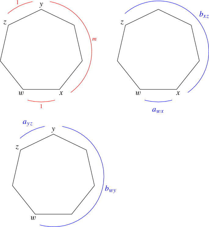
• $a_{wx}b_{xz}=b_{wy}a_{yz}$ for every w, x, y, z in cyclic order with $d(w,x)=1$, $d(x,y)=m$, $d(y,z)=1$.

  

In order to prove the theorem we start by establishing notation. Fix a ‘clockwise’ direction on the vertices of $C_n$.

Definition 7.2

(Codes and admissible simplices)

• Given a vertex x of $C_n$ and $i\in \{-m,\ldots ,0,\ldots ,m\}$, we let $x+i$ denote the vertex obtained by moving |i| places from x, clockwise if $i>0$, and anticlockwise if $i<0$.

• Given a simplex ${\underline{x}}=(x_0,\ldots ,x_k)$, we obtain a sequence $\underline{i}=(i_1,\ldots , i_k)$ with entries in $\{-m,\ldots ,-1,1,\ldots ,m\}$ defined by $x_j = x_{j-1} +i_j$. We call $\underline{i}$ the code of ${\underline{x}}$. Note that the code of a 0-simplex $(x_0)$ is the empty tuple ().

• A code is called admissible if, after dividing it into the maximal subsequences whose entries all have the same sign, the subsequences all have one of the following forms for some $j\geqslant 0$.

  $$\begin{aligned} \underbrace{(1,m,1,m,\ldots )}_{j \text{ entries }} \qquad \underbrace{(-1,-m,-1,-m\ldots )}_{j \text{ entries }} \end{aligned}$$

  Note that while these sequences begin with $\pm 1$, they can end with $\pm 1$ or $\pm m$, according to whether j is odd or even.

• A simplex is admissible if its code is admissible.

Example 7.3

The codes $(1,m,1,-1,1,m)$ and $(1,-1,1,-1)$ are admissible, but (m, 1) and $(-1,-m,1,1,m)$ are not.

Note 7.4

Let ${\underline{x}}=(x_0,\ldots ,x_k)$ be an admissible simplex with code $\underline{i}=(i_1,\ldots ,i_k)$. Then ${\underline{x}}$ has degree k and length $\ell =\sum _{j=1}^k |i_j|$.

Theorem 7.5

(Gu [5]) The admissible simplices ${\underline{x}}$ are cycles in $\mathrm {MC}_{*,*}(C_n)$, and their homology classes $[{\underline{x}}]$ form a basis for $\mathrm {MH}_{*,*}(C_n)$.

This theorem will be crucial for our computations. It has been stated for our own purposes, and does not appear explicitly in [5]. However, it can easily be extracted from the proof of [5, Theorem 4.6], whose ‘unmatched simplices’ are exactly our admissible simplices, and whose final paragraph states that these unmatched simplices form a basis for the homology.

Example 7.6

Let us explore this description in degrees 0, 1, 2.

• The 0-simplices $(x_0)$ are all admissible.

• In degree 1 the admissible codes are (1) and $(-1)$, so the admissible sequences are (x, y) for x, y adjacent, or in other words the oriented edges.

• In degree 2 the admissible simplices are:

  • (x, y, x), one for each oriented edge (x, y). They have length 2. The corresponding codes are $(1,-1)$ and $(-1,1)$.

  • (x, y, z), one for each ordered pair (x, z) with $d(x,z)=m$, where y is determined by the conditions $d(x,y)=1$ and $d(y,z)=m$. They have length $(m+1)$. The corresponding codes are (1, m) and $(-1,-m)$.

Definition 7.7

The universal coefficient sequence of Remark 2.5 gives an isomorphism of $\mathrm {MH}_*^*(C_n)$ with the dual of $\mathrm {MH}_{*,*}(C_n)$, and so we obtain the basis of $\mathrm {MH}_*^*(C_n)$ dual to the one of Theorem 7.5. Using this dual basis we define elements of $\mathrm {MH}_*^*(C_n)$ as follows.

• For each vertex x, $e_x\in \mathrm {MH}_0^0(C_n)$ is the dual to $[(x)]\in \mathrm {MH}_{0,0}(C_n)$.

• For each oriented edge (x, y), $a_{xy}\in \mathrm {MH}^1_1(C_n)$ is the dual to $[(x,y)]\in \mathrm {MH}_{1,1}(C_n)$.

• For each pair x, z with $d(x,z)=m$, $b_{xz}\in \mathrm {MH}^2_{m+1}(C_n)$ denotes the dual to $[(x,y,z)]\in \mathrm {MH}_{2,m+1}(C_n)$. Here y is determined by the conditions $d(x,y)=1$, $d(y,z)=m$ as in Example 7.6.

Lemma 7.8

The relations specified in Theorem 7.1 hold.

Proof

One can check that, under the isomorphism of Theorem 6.2, $e_x$ corresponds to the path x and $a_{xy}$ to the path xy, and the theorem gives us the following relations:

• $e_x^2=e_x$ for every vertex x.

• $e_xe_y=0$ for distinct vertices x, y.

• $a_{xy}=e_xa_{xy}=a_{xy}e_y$ for every oriented edge xy.

• $a_{xy}a_{yz}=0$ if xy and yz are oriented edges with $x\ne z$.

We now prove the relation:

• $b_{xz}=e_xb_{xz}=b_{xz}e_z$ for every x, z with $d(x,z)=m$.

Let $(a_0,a_1,a_2)$ be an admissible simplex. Then $\langle e_x\cdot b_{xy},[(a_0,a_1,a_2)]\rangle = \langle e_x, [(a_0)]\rangle \cdot \langle b_{xy},[(a_0,a_1,a_2)]\rangle$ as one sees by choosing cocycles representing $e_x$ and $b_{xz}$. For $(a_0,a_1,a_2)=(x,y,z)$ both factors evaluate to 1, and for any other choice of $(a_0,a_1,a_2)$ the second factor evaluates to 0, so that $e_x\cdot b_{xz}=b_{xz}$. The other part of the relation is proved similarly. Now we prove the final relation:

• $a_{wx}b_{xz}=b_{wy}a_{yz}$ for every w, x, y, z in cyclic order with $d(w,x)=1$, $d(x,y)=m$, $d(y,z)=1$.

Let $(x_0,x_1,x_2,x_3)$ be an admissible simplex. Then by choosing cocycles representing $a_{wx}$, $b_{xz}$, $b_{wy}$ and $a_{yz}$, we see that

$$\begin{aligned} \langle a_{wx}\cdot b_{xz},[(x_0,x_1,x_2,x_3)]\rangle = \langle a_{wx},[(x_0,x_1)]\rangle \cdot \langle b_{xz},[(x_1,x_2,x_3)]\rangle \end{aligned}$$

and

$$\begin{aligned} \langle b_{wy}\cdot a_{yz},[(x_0,x_1,x_2,x_3)]\rangle = \langle b_{wy},[(x_0,x_1,x_2)]\rangle \cdot \langle a_{yz},[(x_2,x_3)]\rangle . \end{aligned}$$

Notice that in each case the right hand side vanishes unless $x_0=w$, $x_3=z$, and $\ell (x_0,x_1,x_2,x_3)=(m+2)$. The only admissible 3-simplex with these properties is $(x_0,x_1,x_2,x_3)=(w,x,y,z)$, and so it suffices to show that the two right hand sides displayed coincide in this case. This follows from the fact that $\langle a_{wx},[(w,x)]\rangle$, $\langle a_{yz},[(y,z)]\rangle$, $\langle b_{wy},[(w,x,y)]\rangle$ and $\langle b_{xz},[(x,y,z)]\rangle$ are all equal to 1. This is by definition in the first three cases. In the final case, we note that (x, y, z) has code (m, 1), but that if we let $y'$ denote the vertex with $d(x,y')=1$ and $d(y',z)=m$, then $\partial (x,y',y,z)=-(x,y,z)+(x,y',z)$ so that $[(x,y,z)]=[(x,y',z)]$ and consequently $\langle b_{xz},[(x,y,z)]\rangle = \langle b_{xz},[(x,y',z)]\rangle =1$. So both sides of our relation coincide when evaluated on any basis element of $\mathrm {MH}_{3,(m+2)}(C_n)$, and this completes the proof. $\square$

Definition 7.9

(Monomials from admissible tuples) Suppose given an admissible simplex ${\underline{x}}$ with code (), (1), $(-1)$, (1, m) or $(-1,-m)$. Then we define $p_{\underline{x}}\in \mathrm {MH}^*_*(C_n)$ to be the class $e_{x_0}$, $a_{x_0x_1}$ or $b_{x_0x_2}$ dual to $[{\underline{x}}]$. More generally, if ${\underline{x}}=(x_0,\ldots ,x_k)$ is an admissible simplex with $k>0$, then there is a unique way to decompose ${\underline{x}}$ into ‘pieces’

$$\begin{aligned} {\underline{x}}_1=(x_{i_0},\ldots ,x_{i_1}), \ {\underline{x}}_2=(x_{i_1},\ldots ,x_{i_2}), \ \ldots , \ {\underline{x}}_r=(x_{i_{r-1}},\ldots ,x_{i_r}), \end{aligned}$$

with $i_0=0$ and $i_r=k$, such that each piece has code (1), $(-1)$, (1, m) or $(-1,-m)$, and in this case we define $p_{\underline{x}}= p_{{\underline{x}}_1}\cdots p_{{\underline{x}}_r}$.

Example 7.10

An admissible simplex ${\underline{x}}=(x_0,x_1,x_2,x_3,x_2,x_3,x_1)$ with code $(1,m,1,-1,1,m)$ breaks into pieces

$$\begin{aligned} (x_0,x_1,x_2), \quad (x_2,x_3), \quad (x_3,x_2), \quad (x_2,x_3,x_1) \end{aligned}$$

with codes

$$\begin{aligned} (1,m), \quad (1), \quad (-1), \quad (1,m) \end{aligned}$$

respectively, and so the corresponding monomial is $p_{\underline{x}}= b_{x_0x_2}a_{x_2x_3}a_{x_3x_2}b_{x_2x_1}$.

Lemma 7.11

The relations of Theorem 7.1 imply that every monomial in the generators of Theorem 7.1 is either 0, or has the form $p_{\underline{x}}$ for some admissible simplex ${\underline{x}}$.

Proof

Lemma 7.8 shows that the given relations among the generators hold. Using the relations involving the $e_x$, we may ensure that our monomial is either 0, or a single $e_x$, or that the monomial consists entirely of $a$’s and $b$’s. Using the same relations again, we may ensure that the second subscript of each term always coincides with the first subscript of the next term, otherwise we obtain 0 once more. Let us say that $a_{xy}$ is clockwise if x, y are in clockwise order, and anticlockwise otherwise. And let us say that $b_{xz}$ is clockwise if x, z are in anticlockwise order, and anticlockwise otherwise. Now we factor our monomial p into the maximal factors $p_1,\ldots ,p_r$ where each $p_i$ has entries that are all either clockwise or anticlockwise. Our ‘clockwise’ conventions ensure that in each $p_i$, any instance of an $a$ term preceding a $b$ term is an instance of the left-hand-side of the final relation of Theorem 7.1. We may therefore use that final relation to ensure that any $a$ terms occur after any $b$ terms. If we find more than one $a$ term, then $p_i=0$ and so $p=0$. Otherwise, each $p_i$ now has form $p_{{\underline{x}}_i}$ for an appropriate ${\underline{x}}_i$, and consequently $p=p_{\underline{x}}$ where where ${\underline{x}}$ is obtained by combining the ${\underline{x}}_i$. $\square$

Lemma 7.12

Let ${\underline{x}}$ and ${\underline{y}}$ be admissible simplices. Then

$$\begin{aligned} \langle p_{\underline{x}},[{\underline{y}}]\rangle = \left\{ \begin{array}{ll} 1 &{} \text {if }{\underline{x}}={\underline{y}}\\ 0 &{} \text {if }{\underline{x}}\ne {\underline{y}}\end{array} \right. \end{aligned}$$

The $p_{\underline{x}}$ for ${\underline{x}}$ admissible form a basis of $\mathrm {MH}^*_*(C_n)$.

Proof

Suppose ${\underline{x}}={\underline{y}}$. Then, following the definition of the product and the construction of $p_{\underline{x}}$, we find that $\langle p_{\underline{x}},[{\underline{x}}]\rangle =\prod \langle p_{{\underline{x}}_i},[{\underline{x}}_i]\rangle$ where ${\underline{x}}_1,\ldots ,{\underline{x}}_r$ is the decomposition of ${\underline{x}}$ into ‘pieces’ as in Definition 7.9. And by definition, each $\langle p_{{\underline{x}}_i},[{\underline{x}}_i]\rangle$ is equal to 1.

Suppose now that $\langle p_{\underline{x}},[{\underline{y}}]\rangle \ne 0$. We will show that ${\underline{x}}={\underline{y}}$. Decompose ${\underline{x}}$ into ${\underline{x}}_1,\ldots ,{\underline{x}}_r$ as in Definition 7.9, and decompose ${\underline{y}}$ in parallel with ${\underline{x}}$, so that if the pieces for ${\underline{x}}$ are

$$\begin{aligned} {\underline{x}}_1=(x_{i_0},\ldots ,x_{i_1}), \ {\underline{x}}_2=(x_{i_1},\ldots ,x_{i_2}), \ \ldots \ {\underline{x}}_r=(x_{i_{r-1}},\ldots ,x_{i_r}), \end{aligned}$$

then those for y are

$$\begin{aligned} {\underline{y}}_1=(y_{i_0},\ldots ,y_{i_1}), \ {\underline{y}}_2=(y_{i_1},\ldots ,y_{i_2}), \ \ldots \ {\underline{y}}_r=(y_{i_{r-1}},\ldots ,y_{i_r}). \end{aligned}$$

Each of the ${\underline{y}}_i$ is still a cycle, and $\langle p_{\underline{x}},[{\underline{y}}]\rangle =\prod \langle p_{{\underline{x}}_i},[{\underline{y}}_i]\rangle$, so that each $\langle p_{{\underline{x}}_j},[{\underline{y}}_j]\rangle$ must be nonzero, and in particular $x_{i_{j-1}}=y_{i_{j-1}}$ and $x_{i_{j}}=y_{i_{j}}$. If follows that $x_{i_j}=y_{i_j}$ for $j=0,\ldots ,r$. The only way that ${\underline{x}}$ and ${\underline{y}}$ can now differ is that ${\underline{x}}$ and ${\underline{y}}$ may now have pieces ${\underline{x}}_j=(x_{i_{j-1}},x,x_{i_j})$ and ${\underline{y}}_j=(x_{i_{j-1}},y,x_{i_j})$ with codes (1, m) and (m, 1) respectively, or with codes $(-1,-m)$ and $(-m,-1)$ respectively. Let us suppose it is the positive case. Consider the first instance of such a difference. Since ${\underline{y}}$ is admissible, the term preceding (m, 1) in the code of ${\underline{y}}$ must be 1. The same must therefore be true of ${\underline{x}}$, so that the code of ${\underline{x}}$ contains a subsequence (1, 1, m). This is a contradiction, so that ${\underline{x}}$ and ${\underline{y}}$ must coincide. $\square$

Proof of Theorem 7.1

Let $A_*^*$ denote the bigraded ring determined by the presentation in Theorem 7.1. Definition 7.7 and Lemma 7.11 determine a well-defined homomorphism $h:A_*^*\rightarrow \mathrm {MH}_*^*(C_n)$. Definition 7.9 and Lemma 7.11 determine a spanning set (the $p_{\underline{x}}$ for ${\underline{x}}$ admissible) for $A_*^*$, and Lemma 7.12 shows that h sends this spanning set into a basis of $\mathrm {MH}^*_*(C_n)$. It follows that h is an isomorphism. $\square$

References

Crawley-Boevey, W.: Lectures on representations of quivers. (1992)
Eilenberg, S., Lane, S.M.: On the groups \(H(\Pi , n)\). I. Ann. Math. 2(58), 55–106 (1953)
Eilenberg, S., Lane, S.M.: On the groups \(H(\Pi ,n)\). II. Methods of computation. Ann. Math. 60, 49–139 (1954)
Gimperlein, H., Goffeng, M.: On the magnitude function of domains in Euclidean space. Am. J. Math. 143(3), 939–967 (2021)
Gu, Y.: Graph magnitude homology via algebraic morse theory. Preprint, available at arXiv:1809.07240v1, (2018)
Hatcher, A.: Algebraic topology. Cambridge University Press, Cambridge (2002)
Hepworth, R., Willerton, S.: Categorifying the magnitude of a graph. Homol. Homotopy Appl. 19(2), 31–60 (2017)
Jubin, B.: On the magnitude homology of metric spaces. Preprint, available at arXiv:1803.05062, (2018)
Kaneta, R., Yoshinaga, M.: Magnitude homology of metric spaces and order complexes. Bull. Lond. Math. Soc. 53(3), 893–905 (2021)
Leinster, T.: The Euler characteristic of a category. Doc. Math. 13, 21–49 (2008)
Leinster, T.: The magnitude of metric spaces. Doc. Math. 18, 857–905 (2013)
Leinster, T.: The magnitude of a graph. Math. Proc. Cambridge Philos. Soc. 166(2), 247–264 (2019)
Leinster, T., Shulman, M.: Magnitude homology of enriched categories and metric spaces. Algebr. Geom. Topol. 21(5), 2175–2221 (2021)
Otter, N.: Magnitude meets persistence. Homology theories for filtered simplicial sets. Preprint, available at arXiv:1807.01540v1, (2018)
Solow, A.R., Polasky, S.: Measuring biological diversity. Environ. Ecol. Stat. 1, 95–107 (1994)
Weibel, C.A.: An introduction to homological algebra. Cambridge Studies in Advanced Mathematics, vol. 38. Cambridge University Press, Cambridge (1994)
Willerton, S.: Magnitude Homology Reading Seminar, I. Blogpost on the \(n\)-Category Café. https://golem.ph.utexas.edu/category/2018/03/magnitude_homology_reading_sem.html, (2018)
William Lawvere, F.: Metric spaces, generalized logic, and closed categories [Rend. Sem. Mat. Fis. Milano 43 (1973), 135–166 (1974); MR0352214 (50 #4701)]. Repr. Theory Appl. Categ., (1):1–37, 2002. With an author commentary: Enriched categories in the logic of geometry and analysis
William Lawvere, F.: Metric spaces, generalized logic, and closed categories. Rend. Sem. Mat. Fis. Milano 43(135–166), 1973 (1974)
Author information
Authors and Affiliations
Corresponding author
Additional information
Publisher's Note
Springer Nature remains neutral with regard to jurisdictional claims in published maps and institutional affiliations.
Rights and permissions
Open Access This article is licensed under a Creative Commons Attribution 4.0 International License, which permits use, sharing, adaptation, distribution and reproduction in any medium or format, as long as you give appropriate credit to the original author(s) and the source, provide a link to the Creative Commons licence, and indicate if changes were made. The images or other third party material in this article are included in the article’s Creative Commons licence, unless indicated otherwise in a credit line to the material. If material is not included in the article’s Creative Commons licence and your intended use is not permitted by statutory regulation or exceeds the permitted use, you will need to obtain permission directly from the copyright holder. To view a copy of this licence, visit http://creativecommons.org/licenses/by/4.0/.
About this article
Cite this article
Hepworth, R. Magnitude cohomology. Math. Z. 301, 3617–3640 (2022). https://doi.org/10.1007/s00209-022-03013-8
Received:
Accepted:
Published:
Issue Date:
DOI: https://doi.org/10.1007/s00209-022-03013-8