
Abstract
We study the front of the solution to the F-KPP equation with randomized non-linearity. Under suitable assumptions on the randomness including spatial mixing behavior and boundedness, we show that the front of the solution lags at most logarithmically in time behind the front of the solution of the corresponding linearized equation, i.e. the parabolic Anderson model. This can be interpreted as a partial generalization of Bramson’s findings (Bramson in Commun Pure Appl Math 31(5):531–581, 1978) for the homogeneous setting. Partially building on this result and its derivation, we establish functional central limit theorems for the fronts of the solutions to both equations.
1 Introduction and Main Results
1.1 The classical F-KPP equation
The F-KPP equation is the initial value problem given by
with initial condition \(w_0: \mathbb {R}\rightarrow [0,1].\) Its investigation has a long history, with seminal results dating back to Fisher [13] and Kolmogorov–Petrovskii–Piskunov [24]. Their research had been motivated by pioneering works in genetics, where the equation has been used to model a randomly mating diploid population living in a one-dimensional habitat. Further applications can be found in chemical combustion theory or flame propagation, see [1, 12], as well as [37] and references therein.
In [24] it has been shown that for reasonably general non-linearities (see (SC) at the beginning of Sect. 1.4 for further details) and initial conditions of Heaviside type \(w_0=\mathbb {1}_{(-\infty ,0]}\), the solution to (1.1) approaches a traveling wave \(g:\mathbb {R}\rightarrow [0,1]\). I.e., there exists a function \(m: [0,\infty ) \rightarrow \mathbb {R}\)—generally referred to as the (position of the) front or breakpoint—such that
The limit g is known (see [24, Theorems 14 and 17]) to solve the differential equation
and it is unique up to spatial translations. In particular, in this case the first order asymptotics \( m(t)/t {\longrightarrow }_{t\rightarrow \infty } \sqrt{2}\) has been derived. A couple of decades later, Bramson in his seminal work [8] improved this result by computing the second order correction up to additive constants. More precisely, he showed that for each \(\varepsilon \in (0,1),\) the choice \(m(t)=m^\varepsilon (t):=\sup \{x\in \mathbb {R}: w(t,x)=\varepsilon \}\) fulfills
Later on, Bramson [7, Theorem 3 (p. 141)] extended this result to more general initial conditions; roughly speaking, he required the initial condition \(w_0(x)\) to have a sufficiently fast exponential decay for \(x\rightarrow \infty \) and to be non-vanishing for \(x\rightarrow -\infty \). One of the main tools employed in the proof was the McKean representation of the solution to (1.1) in terms of expectations of branching Brownian motion, see [20] and [27]. Another important ingredient was the comparison of the solution of (1.1) to the solution of its linearized version
Indeed, since m(t) describes the front of the solution where u is small and hence \(1-u \approx 1,\) the heuristics is that m(t) is in some sense well-approximated by the front of the solution to (1.3). More precisely, for \(\overline{m}(t):=\sup \{x\in \mathbb {R}: u(t,x)=\varepsilon \}\) and Heaviside-type initial condition \(w_0=\mathbb {1}_{(-\infty ,0]}\), standard Gaussian computations entail
In combination with (1.2), this results in a respective logarithmic backlog of the two fronts in the sense that
The main goal of this article is to investigate the effect of introducing a random potential in the non-linearity of (1.1) as well as in its linearization (1.3), on the logarithmic backlog derived in (1.5) (cf. Theorem 1.5). Taking advantage of this result we will also derive functional central limit theorems for the fronts of the respective solutions to the randomized equations, see Theorem 1.4 and Corollary 1.6 below, which can be interpreted as analogues to homogeneous-case results (1.4) and (1.2).
1.2 The randomized F-KPP equation and the parabolic Anderson model
Already in Fisher’s seminal paper [13], where he investigated the setting (1.1) of homogeneous branching rates, it has been observed that a more realistic model would be obtained by considering spatially heterogeneous rates of the transformation of recessive to advantageous alleles. This, alongside a mathematical interest, is our guiding motivation to consider the setting of random \(\xi \). Replacing the term \(w(1-w)\) of (1.1) by a more general non-linearity F(w) fulfilling suitable standard conditions (see (SC) below), and overriding the notation u and w from the homogeneous setting of the previous section, we then arrive at the equation
as well as its linearized version, the parabolic Anderson model
Here, the stochastic process \(\xi :\mathbb {R}\times \Omega \rightarrow (0,\infty )\) models the random medium; most of the time we will keep the dependence on \(\Omega \) implicit, and write \(\xi \) instead of \(\xi (\cdot , \omega )\) as is common in probability theory. For the case \(F(w)=w(1-w)\) and degenerate \(\xi \equiv 1\), these two equations yield the special cases (1.1) and (1.3), respectively. It has long been known, see e.g. Freidlin [14, Theorem 7.6.1], that under suitable assumptions there exists \(v_0>0\), such that the solution w(t, x) to (F-KPP) converges to 0 (resp. 1), uniformly for all \(x\geqq \overline{v}t\) with \(\overline{v}>v_0\) (resp. for all \(x\leqq \underline{v}t\) with \(\underline{v}<v_0\)), as t tends to infinity. In a similar way, this result can be shown to hold for the solution to (PAM) with the same \(v_0\) as well, showing that the speeds or velocities of both fronts, the one of the solution to (F-KPP) as well as the one of the solution to (PAM), coincide. Consequently, as in the homogeneous case, the question of second order corrections arises naturally.
1.3 Summary of results
In order to address this question and to be able to summarize our results, we introduce some notation. Let \(\varepsilon \in (0,1)\) and \(a>0\). Furthermore, write \(u=u^{\xi ,u_0}\) for the solution to (PAM) with initial condition \(u_0,\) and \(w=w^{\xi ,F,w_0}\) for the solution to (F-KPP) with initial condition \(w_0\). As in the previous section, the fronts of the respective solutions, denoted by
are of special interest. Since we will from now on focus on the heterogeneous setting, we override the notation from Sect. 1.1, where it was used to denote the fronts in the homogeneous case, and define
Our findings are motivated by the respective results of (1.4), (1.2), and (1.5) for the homogeneous case, which provide information about the position of the fronts of the solutions to the respective equations, and thus their respective backlog as well. Under suitable assumptions, our results can be summarized verbally in the following two statements:
-
(a)
There exist a constant \(C \in (0,\infty )\) and a \(\mathbb {P}\)-a.s. finite random time \(\mathcal {T}(\omega )\) such that for all \(t \geqq \mathcal {T}(\omega ),\)
$$\begin{aligned} \overline{m}(t) - m(t) \leqq C \ln t; \end{aligned}$$(1.8)see Theorem 1.5 below.
-
(b)
After centering and diffusive rescaling, the stochastic processes \([0,\infty ) \ni t \rightarrow \overline{m}(t)\) and \([0,\infty ) \ni t \rightarrow m(t)\) satisfy invariance principles; see Theorem 1.4 and Corollary 1.6 below.
As is shown in the companion article [10, Theorems 2.3 and 2.4], in a certain sense there is a logarithmic lower bound for \(\overline{m}(t) - m(t) \) corresponding to (1.8) as well; cf. also Sect. 1.7 below for further discussion.
1.4 Further notation
In order to be able to precisely formulate the previously summarized results, we have to introduce some further notation. We start with introducing the standard conditions for the non-linearity, i.e., F in (F-KPP) has to fulfill the following:
see Fig. 1 for an illustration. Note that the last condition in (SC) is essentially a \(C^{1,1}\)-condition on F at 0. Among others, the conditions in (SC) are used to employ a sandwiching argument for being able to deduce the desired result (1.8) not only for non-linearities F which have the form of a probability generating function, see (PROB) below, but also for all F fulfilling (SC). The sandwiching argument is inspired by the proof of [8, Theorem 2], where the author investigates the homogeneous case \(\xi \equiv \text {const}\).

Sketches of functions fulfilling (SC), all of which are dominated by the identity function
We will now specify the classes of initial conditions under consideration for both, (F-KPP) and (PAM). For this purpose, we fix \(\delta '\in (0,1)\) and \(C'>1,\) and require an initial condition \(u_0\) of (PAM) to fulfill
Our results also hold for initial conditions that decay sufficiently fast at infinity and grow towards minus infinity with sufficiently small exponential rate; i.e., the condition (PAM-INI) can be relaxed to
where \(C \in (0,\infty )\) is a large enough constant. However, in order to avoid further technical complications we stick to the above set of initial conditions.
In addition, let us introduce a tail condition for the initial condition of (F-KPP), which is the same as the one for the case \(\xi \equiv 1\) stated in [7, (1.17)]. For this purpose, we fix \(N,N'>0\), and require \(w_0\) as in (F-KPP) to fulfill
Denote by \(\mathcal {S}^1\) the class of functions \(f:\mathbb {R}\rightarrow [0,\infty )\) which are pointwise limits of increasing sequences of continuous functions, and let
which will be the classes of initial conditions under consideration. An emblematic example which is contained in both, \(\mathcal {I}_{\text {F-KPP}}\) and \(\mathcal {I}_{\text {PAM}},\) is the function \( \mathbb {1}_{(-\infty ,0]}\) of Heaviside type.
We will assume \(\xi =(\xi (x))_{x\in \mathbb {R}}\) to be a stochastic process on a probability space \((\Omega ,\mathcal {F},\mathbb {P})\) having locally Hölder continuous paths, i.e., there exists \(\alpha =\alpha (\xi )>0\) such that for every interval \(I\subset \mathbb {R}\) there exists \(C=C(\xi ,I)>0\), such that

and such that the following conditions are fulfilled:
-
\(\xi \) is uniformly bounded away from 0 and \(\infty \), i.e., there exist constants \(0<\texttt {ei}\leqq \texttt {es}<\infty \) such that \(\mathbb {P}\)-a.s.,
$$\begin{aligned} \texttt {ei}\leqq \xi (x)\leqq \texttt {es}\quad \text { for all }x\in \mathbb {R}; \end{aligned}$$(BDD) -
\(\xi \) is stationary, i.e. for every \(h\in \mathbb {R}\) we have
$$\begin{aligned} (\xi (x))_{x\in \mathbb {R}} \overset{d}{=}\ (\xi (x+h))_{x\in \mathbb {R}}; \end{aligned}$$(STAT) -
\(\xi \) fulfills a \(\psi \)-mixing condition: Let \(\mathcal {F}_x:=\sigma (\xi (z):z\leqq x)\) and \(\mathcal {F}^y:=\sigma (\xi (z):z\geqq y)\), \(x,y\in \mathbb {R}\) and assume that there is a continuous, non-increasing function \(\psi :[0,\infty )\rightarrow [0,\infty )\), such that for all \(j,k\in \mathbb {Z}\) with \(j\leqq k\) as well as \(X\in \mathcal {L}^1(\Omega ,\mathcal {F}_j,\mathbb {P})\) and \(Y\in \mathcal {L}^1(\Omega ,\mathcal {F}^k,\mathbb {P})\) we have
$$\begin{aligned} \big | \mathbb {E}\big [X-\mathbb {E}[X] \, |\, \mathcal {F}^{k}\big ]\big |&\leqq \mathbb {E}[|X|]\cdot \psi (k-j), \nonumber \\ \big | \mathbb {E}\big [Y-\mathbb {E}[Y] \, |\, \mathcal {F}_j\big ]\big |&\leqq \mathbb {E}[|Y|]\cdot \psi ({k-j}), \\ \sum _{k=1}^\infty&\psi (k)<\infty . \nonumber \end{aligned}$$(MIX)Note that (MIX) implies the ergodicity of \(\xi \) with respect to the shift operator \(\theta _y\) acting via \(\xi (\cdot )\circ \theta _y=\xi (\cdot +y)\), \(y\in \mathbb {R}\).
Summarizing, we arrive at the following standing assumptions:
We will provide here two prototypical examples for a suitable potential \(\xi \) satisfying the conditions of (Standing assumptions).
Example 1.1
-
(a)
The Ornstein–Uhlenbeck process \((Y_x)\), \(x \in \mathbb {R},\) is an important stochastic process, which has all the nice properties of being stationary, Markovian, and Gaussian. It can be written as
$$\begin{aligned} Y_x = e^{-x}B_{e^{2x}}, \text { for }\quad x \in \mathbb {R},\quad \text { where }\quad (B_t), t \in [0,\infty ),\quad \text {is a Brownian motion;} \end{aligned}$$(1.9)see Fig. 2 for a realization. For \(0<\varepsilon<M < \infty \) we now consider the potential \(\xi (x) = (\varepsilon \vee Y_x) \wedge M,\) \(x \in \mathbb {R},\) and note that it satisfies (BDD) by definition. It furthermore fulfills (STAT), since the process \((Y_x),\) \(x \in \mathbb {R}\), is stationary. We also note that for any \(\gamma \in (0,1/2)\) the local \(\gamma \)-Hölder continuity of \((Y_x)\) follows from (1.9) in combination with the respective Hölder continuity of Brownian motion (see [28, Corollary 1.20]); hence, (HÖL) holds true. Property (MIX) is somewhat harder to establish. One can for instance do so by taking advantage of the fact that the Ornstein–Uhlenbeck process can also be characterized as the solution to the stochastic differential equation
$$\begin{aligned} \textrm{d}Y_x = -Y_x\, \textrm{d}x + \sqrt{2} \, \textrm{d}B_x, \end{aligned}$$(1.10)and then use the fact that the Ornstein–Uhlenbeck process started from a single point converges to its stationary distribution sufficiently fast (cf. [21, Example 6.8]) as well as the Markov property of the process. The details of the proof are slightly technical and omitted at this point. See [21, 28] for further details on the Ornstein–Uhlenbeck process.
-
(b)
This example is instructive in the sense that not only does it fulfill these conditions, but at the same time it serves as an example in [10] to demonstrate that the transition front of the solution to (F-KPP) can grow logarithmically in time along subsequences in case \(\frac{{\texttt {es}}}{{\texttt {ei}}} > 2\); see [10] for further details. We choose \(0< {\texttt {ei}}<{\texttt {es}}< \infty \) and let \(\chi :[0,\infty ) \rightarrow [0,1]\) be a continuous non-increasing function with \(\chi (x)=1\) for \(x\leqq 1\) and \(\chi (x)=0\) for \(x\geqq 2\), Furthermore, let \(\omega = (\omega ^i)_{i\in \mathbb Z}\) be a Poisson point process on \(\mathbb R\) with homogeneous intensity one. We then define
$$\begin{aligned} \xi (x):={\texttt {ei}}+ ({\texttt {es}}-{\texttt {ei}})\cdot \sup \{ \chi (|x-\omega ^i|):i\in \mathbb Z\}. \end{aligned}$$Observe that by construction the potential \(\xi \) satisfies (HÖL). Furthermore, \(\xi (x)\in [{\texttt {ei}},{\texttt {es}}]\) for all \(x\in \mathbb {R}\), \(\xi (x)={\texttt {ei}}\) if \(|x-\omega ^i|>2\) for all i, and \(\xi (x)={\texttt {es}}\) if there exists \(\omega ^i\) such that \(|x-\omega ^i|\leqq 1\). Also, using the properties of the Poisson point process, it is not hard to show that \(\xi \) fulfills (BDD), (STAT) and (MIX). See Fig. 3 for an illustration of this potential, which highlights the fact that the potential has logarithmically in time long stretches where it equals \({\texttt {ei}}\) that are adjacent to comparably long stretches where it equals \({\texttt {es}};\) cf. [10, Lemma 5.3] for precise statements.

Realization of the potential \(\xi (x) = (\varepsilon \vee Y_x) \wedge M\) with \((Y_x)\), \(x \in \mathbb {R},\) an Ornstein–Uhlenbeck process and the choices \(\varepsilon = 0.25\) and \(M = 1.75\)

Realization of a potential \(\xi \) (top red line) emanating as described from a Poisson point process. This realization exhibits the appearance of long stretches of connected components in space where it takes the values \(\texttt {ei}\) and \(\texttt {es},\) respectively
Since we allow for non-smooth initial conditions in both equations, (F-KPP) and (PAM), we shortly comment on the notion of solution in this setting. We call a function w to (F-KPP) a generalized solution to (F-KPP), if it satisfies
where \(E_x\) is the corresponding expectation of the probability measure \(P_x\), under which \((B_t)_{t\geqq 0}\) is a standard Brownian motion starting in \(x\in \mathbb {R}\). This equation can be interpreted as a mild formulation of (F-KPP) and one can show (see e.g. [14, (1.4), p. 354, and (a), p. 355]) that every classical solution to (F-KPP) also is a generalized one. Generalized solutions can be shown to exist under weak assumptions, and, vice versa, in many instances they turn out to be classical solutions indeed, see Proposition A.9 in Appendix A.
Remark 1.2
A useful observation is that for initial conditions in \(\mathcal {I}_{\text {F-KPP}}\), generalized solutions can be approximated by classical solutions. That is, if \((w_0^{(n)})_{n\in \mathbb {N}}\subset \mathcal {I}_{\text {F-KPP}}\) is a sequence of continuous functions which increase pointwise to \(w_0\), then by Corollary A.11 the corresponding sequence of (by Proposition A.9 classical) solutions \((w^{(n)})_{n\in \mathbb {N}}=(w^{w_0^{(n)}})_{n\in \mathbb {N}}\) to (F-KPP) is also monotone and thus the limit \(w(t,x):=\lim _{n\rightarrow \infty } w^{{(n)}}(t,x)\) exists for all \((t,x)\in [0,\infty )\times \mathbb {R}\). Dominated convergence and the fact that \(w^{(n)}\) also is a generalized solution then imply
I.e., w is the generalized solution to (F-KPP) with initial condition \(w_0\).
A similar concept can be introduced for the solution to (PAM) as well. That is, for \(u_0\in \mathcal {I}_{\text {PAM}}\), we call a function
a generalized solution to (PAM). Note that this is an explicit expression of the solution in terms of a Brownian path, while in (1.11) the solution is only given implicitly. Furthermore, if \(u_0\) is continuous, then by [21, Remark 4.4.4], there exists a unique solution u to (PAM) which fulfills \(u\in C^{1,2}((0,\infty )\times \mathbb {R})\) and \( u(0,\cdot )=u_0.\) As a consequence of these observations, in the following, we will always consider generalized solutions.
1.5 The linearized equation
As already mentioned in the first section, we expect that investigating the solution to (PAM) might also provide some insight into the solution to (F-KPP). Therefore, starting with the first order of the front as a function of time, it turns out useful to consider the so-called Lyapunov exponent
Due to Proposition A.3, the Lyapunov exponent exists \(\mathbb {P}\)-a.s. for all \(v\in \mathbb {R}\), is non-random, and—as a consequence of Corollary 3.10—does not depend on the initial condition in \(\mathcal {I}_{\text {PAM}}\) under consideration. Furthermore, the function \([0,\infty )\ni v\mapsto \Lambda (v)\) is concave, tends to \(-\infty \) as \(v\rightarrow \infty \) and \(\Lambda (0)=\texttt {es}\), where \(\texttt {es}\) is defined in (BDD). \(\Lambda (v)\) describes the asymptotic exponential growth of the solution in the linear regime with speed v. By Proposition A.3, there exists a unique \(v_0>0\) such that
which we will call velocity or speed of the solution to (PAM). Using the properties of the Lyapunov exponent, we immediately infer the first order asymptotics for \(\overline{m}\) to \(\mathbb {P}\text {-a.s.}\) satisfy
It will turn out that our methods work if we require \(v_0\) to be strictly larger than some “critical” value \(v_c\), defined in Lemma 2.4 (d). Roughly speaking, the condition \(v>v_c\) allows for the application of change-of-measure techniques; more precisely, it allows us to find a suitable additive tilting parameter in the exponent of the Feynman–Kac representation (1.12), which depends on v and makes the solution u(t, x) to (PAM) amenable to the investigation by standard tools for values \(x\approx vt\) and large t. Hence, we will work under the assumption
from now on. As will be shown in Sect. 4.4, this assumption is fulfilled for a rich class of potentials \(\xi .\)
We start with investigating the fluctuations of the function \(t \mapsto \ln u(t,vt)\) around \(t\Lambda (v)\) for values v in a neighborhood of \(v_0\), which are interesting in their own right. To this end, on the space \(C([0,\infty ))\) of continuous functions from \([0,\infty )\) to \(\mathbb {R},\) we define the metric
where we write \(\Vert f-g\Vert _j:=\sup _{x\in [0,j]}|f(x)-g(x)|.\) This makes \((C([0,\infty )),\rho )\) a complete separable metric space.
Theorem 1.3
Let (VEL) be fulfilled, \(u_0\in \mathcal {I}_{\text {PAM }},\) and \(u=u^{\xi ,u_0}\) be the corresponding solution to (PAM). Furthermore, let \(V\subset (v_c,\infty )\) be a compact interval such that \(v_0\in \text {int }(V)\). Then for each \(v\in V\), as \(n\rightarrow \infty \) the sequence of random variables \((nv)^{-1/2}\big ( \ln u(n,vn)-n\Lambda (v) \big ),\) \(n \in \mathbb {N},\) converges in \(\mathbb {P}\)-distribution to a centered Gaussian random variable with variance \(\sigma _v^2\in [0, \infty )\), where \(\sigma _v^2\) is defined in (3.1). If \(\sigma _v^2>0\), the sequence of processes
converges as \(n\rightarrow \infty \) in \(\mathbb {P}\)-distribution to a standard Brownian motion in the sense of weak convergence of measures on \(C([0,\infty ))\) endowed with the metric \(\rho \) from (1.15).
Note that in the above one should replace \([0,\infty )\) by \((0,\infty )\) for \(u_0\) such that \([0,\infty ) \ni t \mapsto u(t,vt)\) is not continuous in 0 (the latter might e.g. be the case for \(u_0\) of Heaviside type). In combination with perturbation estimates for u, we will use this result in order to infer an invariance principle for the front of the solution to (PAM). Note that since the function \(t\mapsto \overline{m}_t\) may be discontinuous, we consider convergence in the Skorohod space \(D([0,\infty ))\) in the following result; details on the latter can for example be found in [11].
Theorem 1.4
Let (VEL) be fulfilled, \(u_0\in \mathcal {I}_{\text {PAM }}\) and \(a>0\). Then for \(n \rightarrow \infty ,\) the sequence \(n^{-1/2}\big ( \overline{m}^{\xi ,u_0,a}(n)-v_0n \big ),\) \(n \in \mathbb {N},\) converges in \(\mathbb {P}\)-distribution to a centered Gaussian random variable with variance \(\widetilde{\sigma }_{v_0}^2\in [0,\infty )\), where \(\widetilde{\sigma }_{v_0}^2\) is defined in (3.58). If \(\widetilde{\sigma }_{v_0}^2>0\), the sequence of processes
converges as \(n\rightarrow \infty \) in \(\mathbb {P}\)-distribution to a standard Brownian motion in the Skorohod space \(D([0,\infty ))\).
We underline that in the above theorems the case \(\sigma _v^2=0\) (resp. \(\widetilde{\sigma }_{v_0}^2=0\)) is allowed and leads to a degenerate limit of the corresponding sequences. This can be excluded, e.g. if the finite-dimensional projections of the stochastic process \(\xi =(\xi (x))_{x\in \mathbb {R}}\) are associated (see e.g. [32] or [31] for definitions and results). In this case the covariances in (3.1) are nonnegative and \(\sigma _v^2>0\) follows. Nolen [29, Proposition 2.1] provides an example of a potential, which is generated by an i.i.d. sequence of random variables and thus associated.
1.6 The non-linear equation
Coming back to the original equation of interest, it is natural to ask whether we can obtain results for (F-KPP), which are in some sense counterparts to those derived in latter section for (PAM). For the solution to (F-KPP) it is known (see e.g. [14, §7.6]) that the first order of the position of the front is linear as well and moves with the same velocity as the front of (PAM). Indeed, by Freidlin [14, Theorem 7.6.1] we have that \(\mathbb {P}\text {-a.s.},\)
As mentioned in Sect. 1.2, the next result, which is one of the main results of the paper, states that there is an at most logarithmic distance of the fronts of (F-KPP) and (PAM).
Theorem 1.5
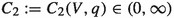
Let (VEL) be fulfilled. Then for each F fulfilling (SC) there exists a constant  such that the following holds: For all \(a>0\), \(\varepsilon \in (0,1)\), \(u_0\in \mathcal {I}_{\text {PAM }}\) and \(w_0\in \mathcal {I}_{\text {F-KPP }},\) there exists a non-random \(C=C(\varepsilon ,a,u_0,w_0)>0\) and a \(\mathbb {P}\text {-a.s.}\) finite random time \(\mathcal {T}=\mathcal {T}(\xi ,\varepsilon ,a,u_0,w_0)\geqq 0\), such that
Moreover for \(w_0=u_0\) and \(a\leqq \varepsilon \), the left inequality in (1.16) can be replaced by \(0 \leqq \overline{m}^{\xi ,u_0,a}(t) - m^{\xi ,F,w_0,\varepsilon }(t) \) for all \(t\geqq 0\).
Furthermore, combining Theorems 1.4 and 1.5, we can deduce an invariance principle for the front of (F-KPP) as well.
Corollary 1.6
Let (VEL) be fulfilled as well as F fulfill (SC), \(w_0\in \mathcal {I}_{\text {F-KPP }}\) and \(\varepsilon \in (0,1)\). Then as \(n \rightarrow \infty ,\) the sequence \(n^{-1/2}\big ( m^{\xi ,F,w_0,\varepsilon }(n)-v_0n \big ),\) \(n \in \mathbb {N},\) converges in \(\mathbb {P}\)-distribution to a centered Gaussian random variable with variance \(\widetilde{\sigma }_{v_0}^2\in [0,\infty )\), where \(\widetilde{\sigma }_{v_0}^2\) is defined in (3.58). If \(\widetilde{\sigma }_{v_0}^2>0\), the sequence of processes
converges as \(n\rightarrow \infty \) in \(\mathbb {P}\)-distribution to a standard Brownian motion in the Skorohod space \(D([0,\infty ))\).
1.7 Discussion and previous results
As already alluded to above, in the homogeneous case (1.1) of constant potential the front has been well-understood by now. This is indeed the case to a much wider extent than illustrated in the Introduction, see e.g. [6] and references therein for further details. Also the heterogeneous setting (F-KPP) of random potential and the properties of its solution have been investigated. Specifically, under fairly general assumptions, the existence and characterization of the propagation speed (i.e., the linear order \(\lim _{t \rightarrow \infty } m(t)/t\) of the position of the front) have been derived by Freidlin and Gärtner, see e.g. [15] as well as [14, Chapter VII], using large deviation principles. Incidentally, the Feynman–Kac formula (see Proposition 2.3 below), which characterizes the solution to the linearization (PAM), has also played an important role in the derivation.
Second order corrections for the position have been investigated by Nolen [29]. Also making the detour along (PAM), he examines (F-KPP) for a potential \(\xi \) under similar assumptions, but requires the (random) initial conditions to satisfy
Here, \(\mathcal {C}_1(\xi )\) and \(\mathcal {C}_2(\xi )\) are positive random variables, and \(g=g^{\xi ,\gamma }\) is a solution to
for \(\gamma >\overline{\gamma }\), for a certain \(\overline{\gamma }>0.\) For technical reasons, he additionally requires \(\gamma <\gamma ^*\), i.e., the initial condition \(w_0(x)\) must not decay too fast as x tends to infinity. The technical assumption (1.17) thus entails being in the supercritical regime which corresponds to waves that move faster than the minimal speed. As his main result, Nolen obtains a (functional) central limit theorem for m(t) in this case also, see [29, Theorem 1.4]. In this lingo, our set of initial conditions corresponds to the critical regime, and Corollary 1.6 (for the critical regime) also suggests that the randomness in Nolen’s central limit theorem is already coming from the environment, and does not necessarily require the randomness of the initial condition.
Furthermore, in [30] a corresponding invariance principle for the front has been derived in the case where the non-linearity in (F-KPP) is either ignition type or bistable.
In [18], on the other hand, for the case of periodic instead of random \(\xi ,\) the authors have investigated the respective logarithmic correction, corresponding to (1.2) in the homogeneous setting; here, the authors have been able to characterize the constant in front of the logarithmic correction as a certain minimizer.
In our main Theorem 1.5, we establish a corresponding logarithmic upper bound for the difference (1.5), also in the setting of a random environment. However, our methods are currently too coarse for identifying a sharp prefactor. Nevertheless, it is a natural question whether the logarithmic upper bound we derive captures the correct order at least. And indeed, in some sense, a partial positive answer to this questions is provided in the companion article [10]. There, the authors show that there exist an increasing sequence \((t_n)\) of times with \(t_n \in (0,\infty )\) such that \(\lim _{n \rightarrow \infty } t_n = \infty \) and a sequence \((x_n)\) of reals such that \(\overline{m}^\frac{1}{2}(t_n) - x_n \geqq c \ln t_n\) such that for all \(n \in \mathbb {N}\) one has
see the discussion around [10, (2.11)] for further details.
As explained above, there is a profound connection between the PDEs we consider and branching Brownian motion, which is more involved than in the setting of constant \(\xi .\) Indeed, related results for branching random walk in random environment (BRWRE) have been recently derived in [9]. In this source the authors analyze the distribution of the maximal particle of a branching random walk in random environment, which itself is closely related to a discrete-space version of (F-KPP). In particular, a corresponding logarithmic upper bound on the distance of the expected position of the maximal particle and the median of the distribution of the maximal particle is given. Furthermore, an invariance principle for the median of the position of the maximal particle of BRWRE is derived. It is therefore no surprise that, on the one hand, principal techniques we employ in this paper are generalizations and adaptations of respective discrete space analogues from [9]. On the other hand, we work under weaker independence assumptions and softer requirements on the non-linearity which we only require to be contained in (SC).
Recall that directly before Theorem 1.3 we have introduced our assumption (VEL), which reads \(v_0 >v_c;\) from a technical point of view, this will be necessary for our change of measure argument to work. It is not hard to show that for a rich class of potentials, this condition is satisfied indeed, cf. Sect. 4.4. What is more, however, in Proposition 4.10 below we also obtain a more profound understanding of the scope of the methods employed. I.e., there exist potentials \(\xi \) fulfilling (Standing assumptions), but such that \(v_0<v_c\) holds true. Therefore, it remains an open and interesting question to understand the behavior of the solutions to the above partial differential equations in case condition (VEL) is not fulfilled.
1.8 Strategy of the proof
Our proofs will be essentially based on techniques from probability theory. One of the principal tools for our investigations is given by the probabilistic representation of solutions to the partial differential equations (PAM) and (F-KPP) through branching Brownian motion in the random (branching) environment \(\xi ;\) the details will be discussed in Sect. 2.1. Further key roles in the proofs of Theorems 1.3 and 1.4 are played by the tilting of probability measures, concentration estimates, as well as perturbation estimates for the solution to (PAM). In the proof of Theorem 1.5 in particular, a modified second moment method will be fundamental. We now provide some further details on the proofs of the main results.
1.8.1 Proof of Theorem 1.3
Considering the initial condition \(u_0 = \mathbb {1}_{(-\infty ,0]}\) for the sake of exposition, the Feynman–Kac formula (1.12) supplies us with
where \(v>0\) stands for velocity. While in probabilistic terms, this expression can be interpreted as the expected number of particles of a branching Brownian motion—starting in vt and with branching rate \(\xi \)—to the left of the origin at time t, we will, after normalization, rather interpret it as a Brownian motion in the random potential \(\xi .\) In this vein, if \(v > v_c,\) then the expectation in (1.19) can be investigated by a random change of measure which depends on the potential \(\xi \), cf. Sect. 2.2, in particular Lemma 2.4. Under this perturbed probability measure, the typical behavior of the Brownian motion in the random potential \(\xi \) (which then has a drift towards the left) started in \(vt\) is to arrive in 0 approximately at time t. Since furthermore the first hitting time of the origin by this Brownian motion is in fact concentrated around t (the respective results can be found in Sect. 3.2), one can take advantage of a resulting renewal structure via independent—but not identically distributed—random variables, which is formulated in terms of empirical Legendre transforms. For a suitably centered and rescaled version of these, one can then show a functional central limit theorem by the use of martingale methods, see Proposition 3.1. Again using Proposition 3.5, one can then infer the desired functional central limit theorem stated in Theorem 1.3; the details are implemented in Sect. 3.3.
1.8.2 Proof of Theorem 1.4
The proof of this result boils down to understanding the behavior of the position of the front \(\overline{m}(t)\) of the solution to (PAM) in dependence on the time t. As already observed in (1.14), to first order it is not hard to observe that the position of the front of the wave is given by \(v_0t.\) Hence, the challenge is to establish the normally distributed second order correction (in functional form). For the purpose of the proof, we can take advantage of the understanding obtained along the proof of Theorem 1.3. More precisely, using perturbation estimates for the solution to (PAM) in time and space which are derived in Sects. 3.4 and 3.5, the functional central limit theorem for the suitably centered and rescaled version of the sequence \([0,\infty ) \ni t \mapsto \ln u(nt,vnt),\) \(n \in \mathbb {N},\) obtained in Theorem 1.3 can be transferred to the functional central limit theorem for the suitably centered and rescaled version of \([0,\infty ) \ni t \mapsto \overline{m}(nt),\) \(n \in \mathbb {N},\) which is the content of Theorem 1.4; see Sect. 3.7 for further details.
1.8.3 Proof of Theorem 1.5
A key difficulty in the proofs stems from the fact that the accuracy up to which we want to understand the behavior of the solutions is logarithmic in time, and hence much smaller than the typical fluctuations of the fronts of the solutions to (PAM) and (F-KPP).
In probabilistic terms, the solution w(t, x) of (F-KPP) with initial condition \(w(0,\cdot ) = \mathbb {1}_{(-\infty ,0]}\) corresponds to the probability that the leftmost particle of the branching Brownian motion in the random environment \(\xi \) is to the left of the origin at time t. As a consequence, proving that the implications of Theorem 1.5 are fulfilled therefore amounts to showing that if one starts at most logarithmically to the left of \(\overline{m}(t),\) the probability of actually seeing a particle to the left of or equal to the origin at time t, is bounded from below by \(\varepsilon .\) In order to do so, we take advantage of a second moment method, see (4.3), to obtain a lower bound on the probability to observe a particle in the branching Brownian motion in the random environment \(\xi \) to the left of the origin at time t. As in the homogeneous setting, such an approach is set to fail when considering all particles in the process; indeed, in this case the second moments would be prohibitively large in comparison to the square of the first moment. Hence, one has to restrict to so-called “leading particles” known from branching Brownian motion in homogeneous branching potential. This notion has to be adapted here in a careful manner so as to cater for the necessities of our random branching potential \(\xi .\) As in the homogeneous case, the remaining steps then boil down to finding good upper bounds for the second moment of leading particles (see Lemma 4.4 in Sect. 4.2) as well as a good lower bound on the first moment of leading particles, cf. Lemma 4.1 in Sect. 4.1; the latter is the harder part in our context. These findings then constitute the main steps in proving Theorem 1.5, the implementation of which is found in Sect. 4.3.
1.9 Notational conventions
We will frequently use sums of real-indexed quantities \(A_x\), \(x\in \mathbb {R}\). In this case, we write
where \(\sum _{i=1}^0:=0\). This notion remains consistent if we also allow for additive constants \(b\in \mathbb {R},\) i.e.
Finally, we set
A prime example is the quantity \(A_{x}= \ln E_x\big [ e^{\int _0^{H_{\lceil x\rceil -1}} (\xi (B_s)-\texttt {es}) \textrm{d}s} \big ]\), where \(H_y:=\inf \{t\geqq 0:B_t=y\}\). Indeed, by the strong Markov property we have \(\ln E_x\big [ e^{\int _0^{H_{0}} (\xi (B_s)-\texttt {es}) \textrm{d}s} \big ]=\sum _{i=1}^{\lfloor x\rfloor }A_i + A_x\) for all \(x\in [0,\infty )\setminus \mathbb {N}_0\).
Furthermore, we will often use positive finite constants \(c_1,c_2,\ldots \) in the proofs. This numbering is consistent within any of the proofs, and it is reset after each proof. On the other hand, \(C_1,C_2,\ldots \) will be used to denote positive finite constants that are fixed throughout the article, and they will oftentimes depend on each other. Other constants like \(c,C, \varepsilon ,\delta \) etc. in the proofs are used to compare certain quantities and are also reset after each proof.
The structure of this article is as follows. In Sect. 2 we will introduce various tools which play a seminal role in our investigations. In particular, these comprise the connections between the partial differential equations under consideration and branching processes, change of measure techniques, as well as concentration inequalities. Taking advantage of these results and further exact large deviation estimates, Sect. 3 first leads to a proof of Theorem 1.3. After developing perturbation results in space and time for the solution to (PAM), Theorem 1.3 will play a crucial role for the proof of Theorem 1.4 as well. The main goal of Sect. 4 then is to show Theorem 1.5, i.e., that the front of the solution to the non-linear equation (F-KPP) lags at most logarithmically in time behind the front of the solution to the linear equation (PAM).
2 Some Technical Tools
In this section we will introduce some further tools that will be helpful in the proof of the main results.
2.1 Connection to branching processes
We define a branching Brownian motion in random environment (BBMRE) as follows: Conditionally on the realization of \(\xi \) and for fixed \(x\in \mathbb {R}\), consider an initial particle starting at a point x and moving as a standard Brownian motion \((B_t)_{t\geqq 0}\) on \(\mathbb {R}\). While at site y, the particle dies at rate \(\xi (y)\). More precisely, for an exponentially distributed random variable S with parameter one, independent of everything else, the first particle dies at time \(\inf \big \{t\geqq 0: S<\int _0^t\xi (B_s)\textrm{d}s \big \}\). When the initial particle dies, it gives birth to k new particles with probability \(p_k\), \(k\in \mathbb {N}\) [see (PROB) below for the precise assumptions on the \(p_k\)]. The new particle(s) start their evolution at the site where their parent particle had died, and they evolve independently of everything else and according to the same stochastic behavior as their parent. Note that on the one hand we assume \(p_0=0\), so genealogies do not die out at any finite time. On the other hand, we allow \(p_1>0,\) i.e., it is possible to die and give birth to one descendant. This implies that a particle at site y branches into more than one particle with rate \(\xi (y)(1-p_1)\). We denote the corresponding probability measure by \(\texttt {P}_x^\xi \) and write \(\texttt {E}_{x}^\xi \) for the respective expectation. By N(t) we denote the set of particles alive at time t. For \(\nu \in N(t)\) we let \((X_s^\nu )_{s\in [0,t]}\) be the spatial trajectory of the genealogy of ancestral particles of \(\nu \) up to time t. For a Borel set \(A\subset \mathbb {R}\) and \(y \in \mathbb {R}\) we define
i.e., the set of particles which are in A at time t, and the number of particles to the left of y at time t.
Let us now introduce a set of functions, formulated in terms of the probability generating function of the sequence \((p_k)_{k\in \mathbb {N}}\) as above. More precisely, assume \((p_k)_{k\in \mathbb {N}}\) and \(F=F^{(p_k)_{k\in \mathbb {N}}}\) to fulfill
Note that such F always fulfills (SC), is smooth and strictly concave on (0, 1). Note that the assumption \(\sum _{k=1}^\infty kp_k = 2\). A fundamental result is the connection of the solution to (F-KPP) and the expected number of particles of the branching process. This is sometimes referred to as the McKean representation. The respective result in the homogeneous setting can be found in [20] as well as [27].
Proposition 2.1
Let \(w_0\in \mathcal {I}_{\text {F-KPP}}\), \(\xi \) satisfy (HÖL), and F fulfill (PROB). Then \(\mathbb {P}\)-a.s. the solution to (F-KPP) is given by
For the proof see Sect. A.5.
Remark 2.2
We will frequently use the application of the latter result to functions \(w_0=\mathbb {1}_{(-\infty ,0]}\), resulting in
Furthermore, we will need the so-called many-to-few lemma, which breaks down the moments of the branching process to a functional of the Brownian paths. For our purposes, it suffices to state it up to second moments (many-to-one and many-to-two formula).
Proposition 2.3
Let \((p_k)_{k\in \mathbb {N}}\) fulfill (PROB) and let \(\varphi _1\), \(\varphi _2: \, [0,\infty ) \rightarrow [-\infty ,\infty ]\) be càdlàg functions satisfying \(\varphi _1\leqq \varphi _2\). Then the first and second moments of the number of particles in N(t) whose genealogy stays between \(\varphi _1\) and \(\varphi _2\) in the time interval [0, t] are given by
and
respectively.
The proof of the first identity follows from [19, Section 4.1]. The second identity can be shown by using [19, Lemma 1], conditioning on the first splitting of the so-called “spines”, similarly to the proof of [16, (2.6)] for \(n=2\) there. Indeed, one has to consider branching Brownian motion instead of branching random walk and replace binary branching by general branching. Then the expectation of the quantity in display [16, (2.15)] turns into the second summand in (FK-2), because the first splitting rate of the two “spine particles” at site y is \((m_2-2)\xi (y)\).
As a consequence of Proposition 2.3, the solution to (PAM) can be expressed by a functional of the branching process, i.e. we have that the solution to (PAM) is given by
As a special case for \(u_0=\mathbb {1}_{(-\infty ,0]}\), this turns into
2.2 Change of measure
As a consequence of, among others, the previous display, it will be important to obtain a profound understanding of Brownian motion in the potential \(\xi .\) For this purpose, we introduce a change of measure which makes it typical for the Brownian motion in the Feynman–Kac formula started at tv, some \(v \ne 0,\) to be close to the origin at time t. This perturbed Brownian motion in the random potential \(\xi \) will then be amenable to an investigation through a certain regeneration structure, as we will show in Sect. 3. More precisely, let \((\xi (x))_{x\in \mathbb {R}}\) be as in (BDD) and define the shifted potential
Then \(\mathbb {P}\)-a.s.,
We will oftentimes write
for the first hitting times and their pairwise differences. The above shift of \(\xi \) gives rise to a change of measure which will play a crucial role in the following. For \(x,y \in \mathbb {R}\) as well as \(\eta \leqq 0\) define the probability measures \(P_{x,y}^{\zeta ,\eta }\) via
with normalizing constant
where \(P_x\) and \(E_x\), \(x\in \mathbb {R}\), are defined below (1.12). For \(A\in \sigma \big (B_{t\wedge H_{x-y}}:t\geqq 0\big )\), using the strong Markov property at time \(H_{x-y}\), we infer that \(P_{x,y}^{\zeta ,\eta }(A)=P_{x,y'}^{\zeta ,\eta }(A)\) for all \(y'\geqq y\). Thus, by the classical Kolmogorov’s extension theorem (see e.g. [36, Theorem 2.4.3]),
We write \(E_x^{\zeta ,\eta }\) for the corresponding expectation and introduce the logarithmic moment generating functions
where we recall the notation introduced in Sect. 1.9, and where the last equality is due to the strong Markov property. In addition, set
Due to (2.3), for any \(\eta \leqq 0\) the quantities above are well-defined, and it is easy to check that in this case and under (BDD), the expressions defined in (2.7)–(2.8) are finite. We have the following useful properties.
Lemma 2.4
-
(a)
The function \((-\infty ,0)\ni \eta \mapsto L(\eta )\) is infinitely differentiable and its derivative \(L'(\eta )\) is positive and monotonically strictly increasing.
-
(b)
We have \(\mathbb {P}\text {-a.s.}\) that
$$\begin{aligned} \lim _{x\rightarrow \infty } \overline{L}_{x}^\zeta (\eta ) = L(\eta )\quad \text {for all }\eta \leqq 0. \end{aligned}$$(2.9) -
(c)
\(L'(\eta )\downarrow 0\) as \(\eta \downarrow -\infty \)
-
(d)
For every \(v>v_c:=\frac{1}{L'(0-)},\) where \(\frac{1}{+\infty }:=0\) and where we call \(v_c\) critical velocity, there exists a
$$\begin{aligned} \text { unique solution}\quad \overline{\eta }(v)<0\quad \text {to the equation } L'( \overline{\eta }(v) ) = \frac{1}{v}. \end{aligned}$$(2.10)\(\overline{\eta }(v)\) can be characterized as the unique maximizer to \((-\infty ,0]\ni \eta \mapsto \frac{\eta }{v} - L(\eta ) \), i.e.
$$\begin{aligned} \sup _{\eta \leqq 0} \Big ( \frac{\eta }{v} - L(\eta ) \Big )= \frac{\overline{\eta }(v)}{v} - L\big ( \overline{\eta }(v) \big ). \end{aligned}$$(2.11)The function \((v_c,\infty )\ni v\mapsto \overline{\eta }(v)\) is continuously differentiable and strictly decreasing.
Proof of Lemma 2.4
-
(a)
This follows from Lemma A.1.
-
(b)
By [14, Theorem 7.5.1], for every \(\eta \leqq 0\) we get \(\mathbb {P}\)-a.s. that \( \lim _{x\rightarrow \infty } \overline{L}^\zeta _x(\eta ) = \mathbb {E}\big [ L_1^\zeta (\eta )\, |\, \mathcal {F}^\zeta _\text {inv} \big ],\) where \( \mathcal {F}^\zeta _\text {inv}\) is the \(\sigma \)-algebra of all \(\mathbb {P}\)-invariant sets. Due to our standing assumptions, the family \(\zeta (x),\) \(x \in \mathbb {R},\) is mixing and thus ergodic. Thus, \( \mathcal {F}^\zeta _\text {inv}\) is \(\mathbb {P}\)-trivial, i.e., \(\mathbb {E}\big [ L_1^\zeta (\eta )\, |\, \mathcal {F}^\zeta _\text {inv} \big ]=L(\eta )\). By continuity of the functions \(\overline{L}^\zeta _x\) and L, the statement follows.
-
(c)
We note that L is strictly increasing and strictly convex on \((-\infty , 0)\) by (a), and that
$$\begin{aligned}L(\eta )\geqq \mathbb {E}\Big [ \ln E_1\big [ e^{-(\texttt {es}-\texttt {ei}-\eta )H_0} \big ] \Big ]= -\sqrt{2(\texttt {es}-\texttt {ei}-\eta )}\quad \text {for all }\eta \leqq 0, \end{aligned}$$where the equality is due to [4, (2.0.1), p. 204]. Thus, we infer that its derivative \(L'(\eta )\) must tend to 0 as \(\eta \rightarrow -\infty \).
-
(d)
Using that \(1/v_c>1/v\) (where \(\frac{1}{0}:=+\infty \)) and the fact that \(L'\) is strictly increasing and continuous with \(L'(\eta )\downarrow 0\) for \(\eta \downarrow -\infty \), we can find a unique \(\overline{\eta }(v)<0\) such that \(L'(\overline{\eta }(v))=1/v\), giving (2.10). Display (2.11) is a direct consequence of (2.10) and standard properties of the Legendre transformations of strictly convex functions. In order to show the remaining part, we observe that since \(L'\) is strictly increasing and smooth on \((-\infty ,0)\), it has a strictly increasing inverse function \((L')^{-1}\), which is differentiable on \((0,1/v_c)\). By (2.10), for \(v>v_c\) we have \(\overline{\eta }(v)=(L')^{-1}(1/v).\) Hence, using the formula for the derivative of the inverse function we get that
$$\begin{aligned} \overline{\eta }'(v)=-\frac{1}{v^2}\cdot \frac{1}{L''(\overline{\eta }(v))}.\end{aligned}$$Since the right-hand side of the latter display is continuous in v and negative, we can conclude.
We use the standard notation \( L^*: \, \mathbb {R}\rightarrow (-\infty , \infty ]\) to denote the Legendre transformation
of L. Lemma 2.4 entails that
In the next part of this section, we are interested in the existence and the properties of a suitable tilting parameter \(\eta _x^\zeta (v)\) such that
holds true (setting \(\eta _x^\zeta (v):=0\) if no such parameter exists). For \(\eta _x^\zeta (v)\) fulfilling (2.13) we observe that under \(P_x^{\zeta ,\eta _x^{\zeta }(v)}\), the Brownian motion is tilted to have time-averaged velocity v until it reaches the origin. More precisely, in Lemma 2.5 we will show that for suitable v and x large enough, a tilting parameter as postulated in (2.13) actually exists. Furthermore, we will show that the random parameter \(\eta _x^\zeta (v)\) concentrates around the deterministic quantity \(\overline{\eta }(v)\) defined in (2.10). The last result is a perturbation estimate for \(\eta _x^\zeta (v)\) in x, cf. Lemma 2.7.
2.3 Concentration inequalities
We have the following result regarding the existence, negativity, and concentration properties of the postulated parameter \(\eta _x^\zeta (v)\).
Lemma 2.5
-
(a)
For every \(v>v_c\) there exists a finite random variable \(\mathcal {N}=\mathcal {N}(v)\) such that for all \(x\geqq \mathcal {N}\) the solution \(\eta _x^\zeta (v)<0\) to (2.13) exists.
-
(b)
For each \(q\in \mathbb {N}\) and each compact interval \(V\subset (v_c,\infty )\), there exists
 such that
  (2.14)
 such that
Proof
We recall that due to Lemma A.1, the tilting parameter \(\eta _x^\zeta (v)\) can alternatively be characterized as the unique solution \(\eta _x^\zeta (v) \in (-\infty ,0)\) to
if the solution exists, and \(\eta _x^\zeta (v)=0\) otherwise. We start with noting that Part (a) directly follows from Part (b). Indeed, let \(A_n\), \(n\in \mathbb {N}\), be the event in the probability on the left-hand side of (2.14). Then \(\sum _n \mathbb {P}(A_n)<\infty \) for \(q\geqq 2\). By the first Borel–Cantelli lemma, \(\mathbb {P}\)-a.s. only finitely many of the \(A_n\) occur. In combination with the fact that \(\overline{\eta }(v) <0\), cf. (2.10), this implies that \(\mathbb {P}\)-a.s., the value of \(\eta _x^\zeta (v)\) can only vanish for \(x>0\) small enough. In particular, we deduce the existence of a \(\mathbb {P}\)-a.s. finite random variable \(\mathcal N\) as postulated.
Hence, it remains to show (2.14). For this purpose, in the following lemma we investigate the fluctuations of the functions through which the parameters \(\eta _x^\zeta (v)\) and \(\overline{\eta }(v)\) are implicitly defined; we will then infer the desired bounds on the fluctuations of the parameters themselves through perturbation estimates for these functions.
Lemma 2.6
For every compact interval \(\triangle \subset (-\infty ,0)\) and each \(q \in \mathbb {N},\) there exists a constant  such that

In order not to hinder the flow of reading, we postpone the proof of this auxiliary result to the end of the proof of Lemma 2.5 and finish the proof of Lemma 2.5 (b) first. Let \(q\in \mathbb {N}\) and \(V\subset (v_c,\infty )\) be a compact interval. By Lemma A.1, for each compact \(\triangle \subset (-\infty ,0)\) we have \(\mathbb {P}\)-a.s.,

Therefore, and because the function \(V\ni v\mapsto \overline{\eta }(v)\) is strictly decreasing by Lemma 2.4, it is possible to find \(N=N(V)\in \mathbb {N}\) and a compact interval \(\triangle =\triangle (N,V) \subset (-\infty ,0),\) where for notational convenience we write
such that, using standard calculus for sets,

Let \(n\geqq N\) and assume that the complement of the event on the left-hand side of (2.16),

occurs. On this event, for all \(v\in V\) and all \(x\in [n,n+1),\)

and thus, due to the strict monotonicity of \((\overline{L}_x^\zeta )'\) as well as its continuity implied by (2.17), there exists a unique \(\eta _x^\zeta (v)\in \triangle \) such that \(\big (\overline{L}_x^\zeta \big )'(\eta _x^\zeta (v))=1/v\). Due to (2.20), still assuming (2.19), we have

Thus, for
\(n\geqq N\), choosing
 , the probability in (2.14) is upper bounded by the right-hand side of (2.16), which finishes the proof.
\(\square \)
, the probability in (2.14) is upper bounded by the right-hand side of (2.16), which finishes the proof.
\(\square \)
It remains to prove Lemma 2.6.
Proof of Lemma 2.6
Applying the strong Markov property at time \(H_{\lfloor x\rfloor },\) we get
Furthermore,
 by (A.1) and Lemma A.1(b), and thus also
 for all
\(x\geqq 1\) and all
\(\eta \in \triangle \),
\(\mathbb {P}\)-a.s. As a consequence, we get that for all
\(x\geqq 1,\)
for all
\(x\geqq 1\) and all
\(\eta \in \triangle \),
\(\mathbb {P}\)-a.s. As a consequence, we get that for all
\(x\geqq 1,\)

It is therefore enough to prove

For each \(\eta \in \triangle \), the sequence \(((L_i^\zeta )'(\eta )-L'(\eta ))_{i\in \mathbb {Z}}\) is a family of stationary, centered and bounded random variables. Furthermore, they fulfill the exponential mixing condition (A.11) due to Lemma A.2. Due to \(\sigma ((L_i^\zeta )'(\eta ):i\geqq k)\subset \sigma (\xi (x):x\geqq k-1)\) and (MIX), setting \(Y_i:=(L_i^\zeta )'(\eta )-L'(\eta )\), the left-hand side in (A.15) is bounded from above by some constant \(c_2>0\), uniformly for every i. Then setting \(m_i:=c_1\), condition (A.15) is fulfilled and we can apply the Hoeffding-type inequality from Corollary A.5 to infer the existence of \(c_2>0\) such that
Let \(\triangle _n := (\triangle \cap \frac{1}{n} \mathbb {Z})\cup \{\eta _*,\eta ^*\}\), recalling the notation of (2.18). Because \(|\triangle \cap \frac{1}{n} \mathbb {Z}|\leqq n\cdot \text {diam}(\triangle )+1\), taking advantage of the previous display we infer
By Lemma A.1(b), we have \(\mathbb {P}\)-a.s. that  . Thus, the mean value theorem entails that

and thus we find  such that (2.21) and hence (2.16) hold true.
In what comes below, many results will implicitly depend on the choice of the compact intervals V and \(\triangle ,\) which have already occurred before. Thus, in order to avoid ambiguity and due to assumption (VEL), we will now
Furthermore, due to Lemma 2.5, there exists a \(\mathbb {P}\)-a.s. finite random variable  such that

We write
for the Legendre transformation of the weighted averages. We also recall that \(\eta _x^\zeta (v)=0\) if there is no solution \(\eta _x^\zeta (v)\in \triangle \) to (2.15); note that this can only happen on \(\mathcal {H}_x^c\).
In order to show an invariance principle for the Legendre transformation \(( \overline{L}_x^\zeta )^*\) in the following section, we now derive a perturbation result on the tilting parameter \(\eta _x^\zeta (v)\) in x.
Lemma 2.7
There exists a constant  such that \(\mathbb {P}\)-a.s., for all \(x \in (0,\infty )\) large enough, uniformly in \(v\in V\) and \(0\leqq h\leqq x\),

Proof
By Lemma 2.5 we can choose x large enough such that \(\eta _y^\zeta (v)\in \triangle \) for all \(y\geqq x\) and all \(v\in V\). For \(h=0\), the statement is obvious. For \(0<h\leqq x\), it suffices to show that there exists \(c_1>0\) such that
Indeed, using (2.15) we can write
for some \(\widetilde{\eta }\in \triangle \) between \(\eta _{x}^\zeta (v)\) and \(\eta _{x+h}^\zeta (v)\). By the second display in (2.17) we know that \(\mathbb {P}\)-a.s.  . Using this, inequality (2.24) is a direct consequence of (2.25) with
  . To prove (2.25), recall that for all \(\eta \in \triangle \), \(x\geqq 1,\) and \(0< h\leqq x,\) by the strong Markov property applied at time \(H_x,\)
Finally, recall that by Lemma A.1 there exists  such that \(\mathbb {P}\)-a.s. we have
  . By exactly the same argument used for the proof of the latter inequality [see proof of (A.1)], one can show that also
  holds \(\mathbb {P}\)-a.s. with the same constant
  . (2.25) now follows choosing
  .
.
3 Functional Central Limit Theorems, Large Deviations and Perturbation Results for the PAM
The principal objective of this section is to establish our first main results, i.e. the functional central limit theorems stated in Theorems 1.3 and 1.4. In order to prepare for this, we start with proving a functional central limit theorem for a suitably centered and rescaled version of the empirical Legendre transforms in Proposition 3.1 of Sect. 3.1. In Sect. 3.2 we then show how this limit theorem can be transferred to an auxiliary quantity \(Y_v^\approx ,\) see Proposition 3.5. In combination with concentration results (referred to as exact large deviations in probability theory) also obtained in Proposition 3.5, we can then deduce that the auxiliary quantity \(Y_v^\approx \) provides a good description of the (Feynman–Kac representation of the) solution to (PAM), see Corollary 3.8 also. In Sect. 3.3 we can then put these findings together to prove Theorem 1.3.
We next obtain perturbation results for the solution to (PAM) in Sects. 3.4 and 3.5. In Sect. 3.7, using the approximation results established in Sect. 3.6 in combination with Theorem 1.3, we can then transfer the latter functional central limit theorem to a functional central limit theorem for the position of the front of the solution to (PAM), hence completing the proof of Theorem 1.4.
3.1 A first functional central limit theorem
We start with a functional central limit theorem for a centered and rescaled version of the empirical Legendre transforms.
For this purpose let
We start with observing that \(\sigma _v^2\in [0,\infty )\) for all \(v\in V\). Indeed, \((\widetilde{L}_i)_{i\in \mathbb {N}}\), where \(\widetilde{L}_i:=L_i^{\zeta }(\overline{\eta }(v))-\mathbb {E}[L_i^{\zeta }(\overline{\eta }(v))]\), is a sequence of bounded (see Lemma A.1), centered and mixing (see Lemma A.2) random variables, giving
where the last inequality is due to uniform boundedness of \(\widetilde{L}_i\) in i, (A.9) and the summability criterion in (MIX). Thus, \(\sigma _v^2\) is well-defined and finite. Furthermore, the non-negativity \(\sigma _v^2\geqq 0\) is due to (3.2) and [34, Lemma 1.1].
We now introduce the process \(W^v_x(t)\) of empirical Legendre transformations
set \(W_0^v(t)=W_x^v(0)=0\) for \(t,x>0\), \(v\in V\), and obtain a first functional central limit theorem for it.
Proposition 3.1
For every \(v \in V\), \(W_n^v(1)\) converges in \(\mathbb {P}\)-distribution to a centered Gaussian random variable with variance \(\sigma _v^2\geqq 0\). If \(\sigma _v^2>0\), the sequence of processes
converges in \(\mathbb {P}\)-distribution to a standard Brownian motion in the sense of weak convergence of measures on \(C([0,\infty )),\) endowed with the topology induced by the metric \(\rho \) from (1.15).
Proof
It is sufficient to show the claim if \((W^v_n(t))_{t\in [0,\infty )}\) is replaced by \((W_n^v(t) \cdot \mathbb {1}_{\mathcal {H}_{nt}})_{t \in [0,\infty )},\) \(n \in \mathbb {N},\) with \(\mathcal H_{nt}\) as defined in (2.23), since the \(\mathbb {P}\)-probability of \(\mathcal H_{nt}\) tends to 1 for \(n\rightarrow \infty \) by Lemma 2.5. In the notation of (3.1), setting
on \(\mathcal {H}_{nt}\) we have
Thus, we can rewrite the relevant term as a sum of three differences
where we note that the third summand vanishes. Indeed, we have
where the last equality is due to (2.11) and the definition of the Legendre transform. The proof is completed by the use of Lemmas 3.3 and 3.2 below, which show that the second summand of (3.5) exhibits the postulated diffusive behavior whereas the first summand is negligible in that scaling.
Lemma 3.2
For every \(v\in V\) and \(t>0\), the sequence of random variables \(\frac{1}{\sqrt{n}}\Big (S_{nt}^{\zeta ,v}(\overline{\eta }(v)) - \mathbb {E}\big [ S_{nt}^{\zeta ,v}(\overline{\eta }(v)) \big ] \Big ),\) \(n \in \mathbb {N},\) converges in \(\mathbb {P}\)-distribution to a centered Gaussian random variable with variance \(\sigma _v^2\geqq 0\). If \(\sigma _v^2>0\), the sequence of processes
converges in \(\mathbb {P}\)-distribution to a standard Brownian motion in the sense of weak convergence of measures on \(C([0,\infty )),\) endowed with the topology induced by the metric \(\rho \) from (1.15).
Proof
Let \(\widetilde{L}_i:=L_i^{\zeta }(\overline{\eta }(v))-\mathbb {E}[L_i^{\zeta }(\overline{\eta }(v))]\), \(\widetilde{V}_i:=V_i^{\zeta }(\overline{\eta }(v))-\mathbb {E}[V_i^{\zeta }(\overline{\eta }(v))]\) and \(M\in \mathbb {N}\). Further set \(\widetilde{L}_i^{(M)}:=\sum _{j=1+(i-1)M}^{iM}\widetilde{L}_j\). Then \((\widetilde{L}_i^{(M)})_{i\in \mathbb {Z}}\) is a sequence of centered, stationary and (by Lemma A.1) bounded random variables. To show the central limit theorem on C([0, M]), we will use the method of martingale approximation from [17], which is summarized as a theorem by Nolen in [29, Section 2.3] and turns out to be applicable in our situation. That is, we have to make sure that condition [29, (2.36)] is fulfilled. Indeed, replacing \(\mathcal {F}^j\) in (A.13) by \(\mathcal {F}_k\) and noting that quantity A in (A.13) is \(\mathcal {F}_k\)-measurable we get
giving the convergence of the first series in [29, (2.36)]. Furthermore, using that \(\widetilde{L}_k^{(M)}\) is \(\mathcal {F}^{(k-1)M}\)-measurable and bounded, also recalling (MIX), we get
Because the series in (3.1) is absolutely convergent, by [34, Lemma 1.1] and [29, (2.37)] we have \(\lim _{n\rightarrow \infty }\frac{1}{n} \mathbb {E}\big [\big (\sum _{k=1}^n\widetilde{L}_k^{(M)}\big )^2\big ]=M\cdot \lim _{n\rightarrow \infty }\frac{1}{Mn} \mathbb {E}\big [\big (\sum _{k=1}^{Mn}\widetilde{L}_k\big )^2\big ]=M\cdot \sigma _v^2\in [0,\infty )\). Furthermore, if \(\sigma _v^2>0\), [29, Theorem 2.1] entails that the sequence of processes
converges in \(\mathbb {P}\)-distribution to a standard Brownian motion \((B_t)_{t\in [0,1]}\) in the sense of weak convergence of measures on C([0, 1]) with the topology induced by the uniform metric. Then by definition, the above convergence also holds true for \((\widetilde{V}_i)_{i\geqq 1}\) instead of \((\widetilde{L}_i)_{i\geqq 1}\). Furthermore, we have the uniform bound
Consequently, the sequence \([0,M]\ni t\mapsto \frac{1}{\sigma _v\sqrt{n}}\Big (S_{nt}^{\zeta ,v}(\overline{\eta }(v)) - \mathbb {E}\big [ S_{nt}^{\zeta ,v}(\overline{\eta }(v)) \big ] \Big )\) has the same weak limit as \(\big (\sqrt{M}\cdot X_n^{(M)}(t/M)\big )_{t\in [0,M]}\), \(n\in \mathbb {N}\), which converges to \(\big (\sqrt{M}\cdot B(t/M)\big )_{t\in [0,M]}\) and the latter process is a standard Brownian motion on [0, M]. Because \(M\in \mathbb {N}\) was arbitrary, Whitt [38, Theorem 5] gives weak convergence on \(C([0,\infty ))\).
To show that the first summand in (3.5) is asymptotically negligible, we use the following result.
Lemma 3.3
There exists a constant  such that for every \(v\in V\) and \(M>0\),

Proof
There exists a \(\mathbb {P}\)-a.s. finite time  , defined before (2.23), such that for all
  and all \(v\in V\) we have \(\eta _x^\zeta (v)\in \triangle \). Furthermore, by Lemma A.1, \(S_{x}^{\zeta ,v}\) is infinitely differentiable on \((-\infty ,0)\), so for all
  there exists \(\widetilde{\eta }_x^\zeta (v) \in [\overline{\eta }(v) \wedge \eta _{x}^\zeta (v), \overline{\eta }(v) \vee \eta _{x}^\zeta (v)]\) such that
Due to (2.15), \((S_x^{\zeta ,v})'(\eta _x^{\zeta }(v))=0\) and by Lemma A.1 we have \(\sup _{\eta \in \triangle }\sup _{x\geqq 1}\big |(S_x^{\zeta ,v})''(\eta )\big |/x\leqq c_1\). By (2.14) and the first Borel–Cantelli lemma, there exists a finite random variable  such that for \(x\geqq \mathcal {N}_2\) the complementary event on the left-hand side of (2.14) occurs, hence

and thus

with  . Finally, we have

where in the last inequality we used that \(\mathbb {P}\)-a.s., every summand in the definition of \(S_n^{\zeta ,\eta }\) is uniformly bounded by \(c_2\). The \(\mathbb {P}\)-a.s. finiteness of  gives the claim.
As a by-product of the proof above we get an approximation result of \(W_x^v\) be a centered stationary sequence.
Corollary 3.4
For every \(v\in V\) and all t such that  we have

Proof
By the definition of \(W^v_x(t)\) and \(S_x^{\zeta ,v}(\eta )\) from (3.3) and (3.4), as well as the definition in (2.12) for the corresponding Legendre transformations, we have
Then we can conclude using (3.6).
3.2 An exact large deviation result for auxiliary processes
The main result of this subsection is Proposition 3.5, where we show—cf. (3.10)—that the probability for the perturbed Brownian motion in shifted potential to hit the origin at time x/v for the first time exhibits certain concentration properties. These concentration properties then allow us to investigate \(Y_v^\approx \) instead of \(Y_v,\) see (3.7) and (3.9) below. The virtue of \(Y_v^\approx \) is that we will be able to employ Proposition 3.1 to deduce a functional central limit theorem for the process induced by it, see also (3.22) below. This again will be beneficial since \(Y_v^\approx \) provides a good description of the (Feynman–Kac representation of the) solution to (PAM), see Corollary 3.8 below.
For \(x\geqq 0\) and \(v>0\) we introduce
where \(K>0\) is a constant, defined in (3.17) below. For \(v\in V\) and \(x\geqq 1\) we define the random quantity
Furthermore, by Lemma A.1, there exists some \(C_{18}>1\) such that  for all \(x\geqq 1\). Thus, there is some constant
  such that

We now prove the following result.
Proposition 3.5
Let V be as in (2.22), \(\sigma _v\) defined by (3.1) and \(W^v_x(t)\) as in (3.3), \(v\in V\), and \(K>0\) be such that (3.17) holds. Then there exists a constant  , such that for all \(v\in V\) and all \(x\geqq 1\), on \(\mathcal {H}_x\) we have

Furthermore, for all \(v\in V\) and all \(x\geqq 1\), on \(\mathcal {H}_{x}\) we have

and the sequence \(n^{-1/2}\big ( \ln Y^\approx _v(n)-nL^*(1/v) \big )\), \(n\in \mathbb {N}\), converges to a centered Gaussian random variable with variance \(\sigma _v^2\in [0,\infty )\), where \(\sigma _v^2\) is defined in (3.1). If furthermore \(\sigma _v^2>0\), then the sequence of processes
converges in \(\mathbb {P}\)-distribution to standard Brownian motion in \(C([0,\infty ))\).
Proof
We start with proving (3.9) and for this purpose let \(x\geqq 1\) such that \(\mathcal {H}_{\lfloor x\rfloor }\) occurs. Write \(\eta :=\eta _{x}^\zeta (v)\) and \(\sigma :=\sigma _x^\zeta (v),\) and recall the notation introduced in (2.4), i.e. \(\tau _i=H_i-H_{i-1}\), \(i=1,\ldots ,\lceil x\rceil -1\), and set \(\tau _x:= H_{\lceil x\rceil - 1} - H_x,\) \(x \in \mathbb {R}\backslash \mathbb {Z}\), (which is consistent with the definition in (2.4) for x integer) to define \(\widehat{\tau }_{i}:={\widehat{\tau }}^{(x)}_{i}:=\tau _{i} - E_x^{\zeta ,\eta }\left[ \tau _{i}\right] \). Then \(\sum _{i=1}^x E_x^{\zeta ,\eta }\left[ \tau _{i} \right] =E_x^{\zeta ,\eta }\left[ H_{0} \right] =\frac{x}{v}\). We now rewrite
Analogously, we get
We define \(\mu _x^{\zeta ,v}\) as the distribution of \(\frac{\eta }{\sigma }\sum _{i=1}^x\widehat{\tau }_i\) under \(P_x^{\zeta ,\eta }\). Then
and
Using Lemma 3.6 below, the integrals on the right-hand side of (3.13) and (3.14), multiplied by \(\sigma \), are bounded from below and above by positive constants. Display (3.9) now follows by the definition of \(W_x^v,\) and (3.10) is a direct consequence of (3.13)–(3.16). The last two statements, are a consequence of (3.9), (3.10), \(W_{nt}^v(1)=\frac{1}{\sqrt{t}} W_n^v(t)\) and Proposition 3.1.
To complete the previous proof, it remains to prove the following.
Lemma 3.6
Under the conditions of Proposition 3.5, there exists a constant  such that for all \(v\in V\) and \(x\geqq 1\), on \(\mathcal {H}_x,\)

and

with \(\mu _x^{\zeta ,v}\) as in the proof of Proposition 3.5.
Proof
We write \(n:=\lceil x\rceil \) and recall that under \(P_x^{\zeta ,\eta }\), the sequence \(\Big (\sqrt{n}\frac{\eta _x^\zeta (v)}{\sigma _x^\zeta (v)}\widehat{\tau }_i\Big )_{i=1,\ldots ,\lfloor x\rfloor ,x}\) is a sequence of independent, centered random variables. Thus, on \(\mathcal {H}_x\) we obtain
Additionally, the \(\widehat{\tau }_i\), \(i \in \mathbb {N},\) have uniform exponential moments. Thus, the conditions of [3, Theorem 13.3] are fulfilled and an application of [3, (13.43)] yields
where the supremum is taken over all Borel-measurable convex subsets of \(\mathbb {R}\), \(\Phi \) denotes the standard Gaussian measure on \(\mathbb {R}\) and \(c_1\) only depends on the uniform bound of the exponential moments of the \(\widehat{\tau }_i,\) \(i \in \mathbb {N}.\) Without loss of generality, we will assume \(c_1>4\). Then, due to (3.8), by denoting \(\mathcal {C}:=\big [0,-K\eta _{x}^\zeta (v)/{\sigma _x^\zeta (v)}\big ]\) we can choose \(K>0\) large enough, so that
We thus get
Because the integrand in (3.15) is bounded away from 0 and infinity on the respective interval of integration (uniformly in \(n \in \mathbb {N}\)), (3.15) is a direct consequence of (3.8) and (3.18). For (3.16), we split the integral into a sum:

where we recall the notation from (2.18). The lower bound in (3.16) can be obtained by noting that
Analogously to (3.18), choosing  large enough, the last expression is bounded from below by
  . Combining this with (3.8), we finally arrive at (3.16).
We are now in the position to prove the following result.
Lemma 3.7
Under the conditions of Proposition 3.5, for each \(\delta >0\) there exists a constant  such that for all \(v\in V\), \(t>0\), on \(\mathcal {H}_{vt}\) we have

Proof
The second inequality is obvious. Since \(\{B_{t}\leqq 0\}\subset \{ H_0\leqq t \}\) and \(\zeta \leqq 0\), we get  by Proposition 3.5 and thus the last inequality in (3.19) is obtained. Therefore, it remains to show the first inequality. For this purpose, define the random function \(p(s):=E_0\big [ e^{\int _0^s\zeta (B_r)\textrm{d}r};B_s\in [-\delta ,0] \big ]\) which almost surely is bounded from below by a deterministic constant \(c_1(K,\delta )>0\) for all \(s\in [0,K]\). Using the strong Markov property at \(H_0\), we finally get
and the claim follows by choosing  .
.
Plugging the relation \(\xi (x)=\zeta (x)+\texttt {es}\), \(x\in \mathbb {R}\), into Lemma 3.7 immediately supplies us with the following corollary.
Corollary 3.8
Let  be as in Lemma 3.7. Then for all \(v\in V\), \(t>0\), on \(\mathcal {H}_{vt}\) we have

Using the Feynman–Kac formula (1.12), Lemma 3.7 also directly entails the following result; recall that \(u^{u_0}\) denotes the solution to (PAM) with initial condition \(u_0\in \mathcal {I}_{\text {PAM}}\).
Corollary 3.9
Let  be as in Lemma 3.7. Then for all \(v\in V\), \(t>0\), on \(\mathcal {H}_{vt}\) we have

The previous results are fundamental for proving perturbation statements in the next section, which themselves will allow us to analyze path probabilities of the branching process.
3.3 Proof of Theorem 1.3
The previous findings already enable us to prove our first main result.
Proof of Theorem 1.3
We first assume \(\sigma _v^2>0\) and consider the case \(u_0=\mathbb {1}_{(-\infty ,0]}\) to show the second part of the claim, i.e. that the sequence of processes
converges in \(\mathbb {P}\)-distribution to standard Brownian motion. Because \([0,\infty ) \ni t\mapsto \ln u(t,vt)\) might be discontinuous only 0 (in which case we replace [0, \(\infty \)) by (0, \(\infty \)) in (3.20)), we cover both cases (continuous and discontinuous in 0) in a unified setting by showing the invariance principle for a sequence of auxiliary processes \((X_n^v(t))_{t\geqq 0}\), \(n\in \mathbb {N}\), where for every \(n\in \mathbb {N}\) and \(t\geqq \frac{1}{n},\) the term \(X_n^v(t)\) is the same as in (3.20), whereas for \(t\in [0,1/n]\) the term \(\ln u(nt,vnt)\) in (3.20) is replaced by \((1-nt)\ln u(0,0) + nt \textrm{ln}~ u(1,v)\), making \((X_n^v(t))_{t\geqq 0}\) continuous. Because the difference of the processes in (3.20) and \((X_n^v (t))_{t\geqq 0}\) converges uniformly to zero as \(n\rightarrow \infty \), convergence of the processes in (3.20) to a standard Brownian motion is equivalent to the convergence of the processes \((X_n^v (t))_{t\geqq 0}\), \(n\in \mathbb {N}\), to a standard Brownian motion in C([0, \(\infty \))) (or C((0, \(\infty \))) in case of a discontinuity in 0) with topology induced by the metric \(\rho \) from (1.15).
By Proposition 3.5 and Corollary 3.8, on \(\mathcal {H}_{nvt}\) (recall the notation from (2.23)) we have

Recall that a sequence of processes \(t\mapsto A_n(t)\), \(n\in \mathbb {N}\), converges in \(\mathbb {P}\)-distribution to standard Brownian motion if and only if for each \(c>0\) the sequence \(t\mapsto c^{-1} A_n(c^2 t)\), \(n\in \mathbb {N}\), converges in \(\mathbb {P}\)-distribution to a standard Brownian motion. Applying this to (3.11), the sequence of processes
converges in \(\mathbb {P}\)-distribution to a standard Brownian motion. Further, by the second line in (3.21),

holds. Consequently, if we can prove that
the claim follows from (3.22). To prove (3.23), we set \(n=1\) in (3.21) and note that \(\frac{W_{vt}^v(1)}{\sqrt{t}}\mathop {\longrightarrow }\limits _{t\rightarrow \infty }0\) \(\mathbb {P}\)-a.s. for all \(v\in V\), because \(W_n(1)\) converges in \(\mathbb {P}\)-distribution to a centered normally distributed random variable by Proposition 3.1. Using (3.25), (3.21) and (3.8), we get (3.23).
It remains to show the claim for arbitrary \(u_0\in \mathcal {I}_{\text {PAM}}\). Recall that there exist \(\delta '\in (0,1)\) and \(C'>1\), such that \(\delta ' \mathbb {1}_{[-\delta ',0]}(x) \leqq u_0(x)\leqq C' \mathbb {1}_{(-\infty ,0]}(x)\) for all \(x\in \mathbb {R}\). Therefore, using Corollary 3.9 we have

where we used that the solution to (PAM) is linear in its initial condition. Thus, the convergence of (3.20) for arbitrary initial condition \(u_0\in \mathcal {I}_{\text {PAM}}\) follows from the convergence with initial condition \(\mathbb {1}_{(-\infty ,0]}\). This gives the second part of Theorem 1.3.
It remains to show that \((nv)^{-1/2}\big ( \ln u(n,vn)-n\Lambda (v) \big )\) converges in \(\mathbb {P}\)-distribution to a Gaussian random variable. For \(u_0=\mathbb {1}_{(-\infty ,0]},\) this is a direct consequence of (3.21) for \(t=1\), (3.23) and the second part of Proposition 3.5. For general \(u_0,\) the claim follows from (3.24).
In view of Corollary 3.9, Proposition A.3 and (3.23), the Lyapunov exponent \(\Lambda \), defined in (1.13), determines the exponential decay (growth, resp.) for solutions to (PAM) for arbitrary initial conditions \(u_0\in \mathcal {I}_{\text {PAM}}\) (and not only for those with compact support).
Corollary 3.10
For all \(v\geqq 0\) and all \(u_0\in \mathcal {I}_{\text {PAM}}\) we have that \(\mathbb {P}\)-a.s.,
Furthermore, \(\Lambda \) is linear on \([0,v_c]\) and strictly concave on \((v_c,\infty ),\) and the convergence in (3.25) holds uniformly on any compact interval \(K\subset [0,\infty )\).
Proof
Note that by Proposition A.3, \(\delta '\mathbb {1}_{[-\delta ',0]}\leqq u_0\leqq C'\mathbb {1}_{ (-\infty ,0] }\) and Corollary 3.9 we have that (3.25) holds for all \(v\in V\) and all compact \(V\subset (v_c,\infty ),\) so (3.25) is true for all \(v>v_c\). The strict concavity of \(\Lambda \) on \((v_c,\infty )\) follows from the strict convexity of \(L^*(1/v)\), which in turn follows from the strict convexity of L and standard properties of the Legendre transformation. If \(v_c=0\), the proof is complete due to \(\lim _{t \rightarrow \infty } \frac{1}{t}\ln u^{\delta '\mathbb {1}_{[-\delta ',0]}}=\Lambda (0)=\texttt {es}\) by Proposition A.3 and \(u^{u_0}\leqq e^{\texttt {es}t}\) for all \(u_0\in \mathcal {I}_{\text {PAM}}\). Thus, let us assume \(v_c>0\) from now on. First observe that \(L^*(1/v)\) tends to \(L^*(1/v_c)=-L(0)\) as \(v\downarrow v_c\). Indeed, due to Lemma 2.4 (d), for each \(v>v_c\) there exists a unique \(\overline{\eta }(v)\in (-\infty ,0),\) characterized via \(L'\big (\overline{\eta }(v)\big )=\frac{1}{v}\), such that \( L^*(1/v)=\frac{\overline{\eta }(v)}{v}-L(\overline{\eta }(v)). \) Furthermore, \((v_c,\infty )\ni v \mapsto \overline{\eta }(v)\) is continuously differentiable and strictly decreasing, bounded from above by 0. In addition, \((-\infty ,0)\ni \eta \mapsto L'(\eta )\) is smooth and strictly monotone and tends to \(L'(0-)\) as \(\eta \uparrow 0.\) As a consequence, we get that \(\eta (v)\uparrow 0\) as \(v\downarrow v_c\) and thus \(L^*(1/v) \rightarrow L^*(1/v_c)\) as \(v\downarrow v_c\). Therefore, we deduce that \(\Lambda (v)=\texttt {es}- vL^*(1/v)\) for all \(v\in [v_c,\infty )\). Furthermore, due to (BDD), for all \(u_0\in \mathcal {I}_{\text {PAM}}\) we have
Using Lemma 2.4 (b), taking logarithms, and dividing by t, we get that the (due to Proposition A.3) concave function \(\Lambda \) is bounded from above by the linear function \([0,\infty )\ni v\mapsto \texttt {es}-vL(0)=\texttt {es}+ vL^*(1/v_c)\) and coincides with this function at \(v=0\) as well as \(v=v_c,\) and hence on the whole interval \([0,v_c]\). Using (3.26) again, we infer (3.25) for all \(v \geqq 0\) and \(u_0\in \mathcal {I}_{\text {PAM}}\).
To show that the convergence is uniform on every compact interval \(K\subset [0,\infty )\), for \(\varepsilon >0\) arbitrary we consider \(\varepsilon \mathbb {Z}:=\{ k\varepsilon :k\in \mathbb {Z}\},\) and for \(y\in \mathbb {R}\) set \(\lfloor {y}\rfloor _{\varepsilon }:=\sup \{ x\in \varepsilon \mathbb {Z}:\, x\leqq y \}\). Then the convergence is uniform on \( K\cap \varepsilon \mathbb {Z}.\) A fortiori, for t large enough, uniformly in \(y\in K\),
Lemma A.8 then entails that

Furthermore, using \(0\leqq y-\lfloor {y}\rfloor _{\varepsilon }\leqq \varepsilon \), we have
Using the Feynman–Kac formula in the equality, the Markov property at time \(\varepsilon t,\) and (BDD) in the first inequality, we infer that
where in the last inequality we used (3.27) and (3.28). Setting \({t}':=t+1+\varepsilon t\) and \({y}':=\frac{{t}'}{t}y\), we get
Since (3.29) holds uniformly for all \(y\in K\), we infer that
Since \(\Lambda \) is concave and finite, it is uniformly continuous on compact intervals. As a consequence, since \(\varepsilon >0\) was chosen arbitrarily, we deduce the lower bound
To derive the matching upper bound, we assume that the convergence does not hold uniformly on K. Then, due to (3.30), there exist \(\alpha >0\) and sequences \((t_n)_{n\in \mathbb {N}}\subset [0,\infty )\) and \((y_n)_{n\in \mathbb {N}}\subset K\) such that \(t_n\rightarrow \infty \) and
Retreating to a suitable subsequence, we can assume \(y_{n}{\longrightarrow }_{n\rightarrow \infty } y\in K.\) For n such that \(|y_n-y|\leqq \varepsilon \), we have, similarly to (3.28),
Therefore, taking advantage of (3.27) again and using an argument as in the derivation of (3.29), we infer that
for all n such that \(|y_n-y|\leqq \varepsilon \). Now recall that \(y_n{\longrightarrow }_{n\rightarrow \infty } y\), that \(\Lambda \) is continuous, as well as \(\frac{1}{t}\ln u(t,ty){\longrightarrow }_{t\rightarrow \infty }\Lambda (y).\) Therefore, first taking logarithms, dividing by \(t_n\), and then taking \(n \rightarrow \infty ,\) the left-hand side in (3.32) converges to \((1+\varepsilon )\Lambda (y).\) Contrarily, by (3.31), the limit of the right-hand side is bounded from below by \( \Lambda (y)+\alpha +\varepsilon \texttt {ei}- \frac{(1+y)^2}{2}\varepsilon \). Choosing \(\varepsilon >0\) small enough, this leads to a contradiction. As a consequence, we deduce the uniform convergence on K.
3.4 Time perturbation
In the next step we prove perturbation results, i.e., the time and space perturbation Lemmas 3.11 and 3.12. These statements will be useful when comparing the expected number of particles of the BBMRE which are slightly slower or faster than the ones with given velocity. As usual, \(u=u^{u_0}\) denotes the solution to (PAM) with initial condition \(u_0\in \mathcal {I}_{\text {PAM}}\).
Lemma 3.11
-
(a)
Let \(u_0\in \mathcal {I}_{\text {PAM}}\) and let \(\varepsilon : \, (0,\infty ) \rightarrow (0,\infty )\) be a function such that \(\varepsilon (t)\rightarrow 0\) and \(t\varepsilon (t)\rightarrow \infty \) as \(t\rightarrow \infty \). Then there exists
 such that \(\mathbb {P}\)-a.s., for all t large enough,
  (3.33)
where \(\mathcal {E}_t:=\left\{ (v,h):\ v\in V,\ |h|\leqq t\varepsilon (t),\frac{vt}{t+h}\in V \right\} \).
-
(b)
For all \(\varepsilon >0\) and \(u_0\in \mathcal {I}_{\text {PAM}}\) there exists a constant
 and a \(\mathbb {P}\)-a.s. finite random variable
  such that for all
  , uniformly in \(0\leqq h\leqq t^{1-\varepsilon }\), \(v\in V\) and \(\frac{vt}{t+h}\in V,\)
 (3.34)
 such that
 and a
and a  such that for all
  , uniformly in
Proof
(a) Note that it suffices to show the claim for \(u_0=\mathbb {1}_{(-\infty ,0]}\). Indeed, for all \(u_0\in \mathcal {I}_{\text {PAM}}\) we have \(\delta '\mathbb {1}_{[-\delta ',0]}\leqq u_0\leqq C'\mathbb {1}_{(-\infty ,0]}\). Using Corollary 3.9, we infer that for all \(u_0\in \mathcal {I}_{\text {PAM}}\), all \(v\in V,\) and all t large enough

where \(u^{u_0}\) denotes the solution to (PAM) with initial condition \(u_0\).
by the same argument as at the end of the proof of Theorem 1.3, the solutions to (PAM) for different initial conditions \(u_0\in \mathcal {I}_{\text {PAM}}\) differ at most by a multiplicative constant. Let t be large enough such that \(\mathcal {H}_{vt}\) occurs for all \(v\in V\), which is possible by (2.23). Letting \((v,h)\in \mathcal {E}_t\) and writing \(v':=\frac{vt}{t+h}\in V,\) we infer that
Using Lemma 3.7, on \(\mathcal {H}_{vt},\) the last fraction divided by \(\frac{Y_{v'}^\approx (vt)}{Y_{v}^\approx (vt)}\) is bounded away from 0 and infinity for all t large enough. As in the derivation of (3.12), the term \(\frac{Y_{v'}^\approx (vt)}{Y_{v}^\approx (vt)}\) can be written as
where \(\widehat{\tau }_i=\tau _i - E_{vt}^{\zeta ,\eta _{vt}^\zeta (v')}[\tau _i]\) and \(\widetilde{\tau _i}:=\tau _i - E_{vt}^{\zeta ,\eta _{vt}^\zeta (v)}[\tau _i]\). But now, since \(v'\in V,\) as in the proof of Proposition 3.5, the first fraction of the previous display is bounded from below and above by positive constants, for all t large enough. Indeed, setting \(x=vt\) in (3.13), the denominator in (3.36) equals the integral in (3.13) and, replacing v by \(v'\) in (3.13), the numerator equals the integral in (3.13). The claim then follows due to Lemma 3.6 and using (3.8). Therefore, taking logarithms in (3.35) and recalling the definition of \(S_{vt}^{\zeta ,v}(\eta )\) in (3.4), according to the previous considerations it suffices to show that the logarithm of the second fraction in (3.36) plus \(\overline{\eta }(v)\cdot h\), i.e.
satisfies bound on the right-hand side of (3.33), uniformly in \((v,h)\in \mathcal {E}_t\). Recall that \(\frac{1}{v'}=\frac{1}{v}\left( 1+\frac{h}{t} \right) \), thus the second summand in (3.37) is \(-h\cdot \eta _{vt}^\zeta (v')\). The triangle inequality entails
and so by Lemma 2.5, uniformly for \(v'\in V\) and t large enough, the first term on the right-hand side of (3.38) can be upper bounded by  , \(\mathbb {P}\)-a.s. Furthermore, by Lemma 2.4(d) we know that \(\overline{\eta }\) is continuously differentiable and strictly decreasing, having uniform positive bounds of the derivative on every bounded subinterval of \((v_c,\infty )\). Hence, \(\overline{\eta }(\cdot )\) is Lipschitz continuous on V and we therefore get that the second summand in (3.38) can be upper bounded by \(c_1|v-v'|=c_1v\frac{|h|}{|t+h|}=c_1v\frac{|h|}{t}\cdot \frac{t}{|t+h|}\leqq c_2 \frac{|h|}{t}\), uniformly for all \(v,v'\in V\) and all t large enough, where the last inequality is due to \(|h|/t\leqq \varepsilon (t)\rightarrow 0\). Therefore, the absolute value of the sum of the second and third summand in (3.37) is upper bounded by
  with
with  .
.
It remains to show that the first summand in (3.37) tends to 0 as t tends to \(\infty \). We write
for some \(\widetilde{\eta } \in [\eta _{vt}^{\zeta }(v') \wedge \eta _{vt}^{\zeta }(v), \eta _{vt}^{\zeta }(v') \vee \eta _{vt}^{\zeta }(v)]\). Recall that \(S_{vt}^{\zeta ,v}(\eta )=vt\big (\frac{\eta }{v}-\overline{L}_{vt}^\zeta (\eta )\big )\) and by definition \(\big (\overline{L}_{vt}^\zeta \big )'\big (\eta _{vt}^\zeta (v)\big ) = \frac{1}{v}\). Thus, \( \big (S_{vt}^{\zeta ,v}\big )'(\eta _{vt}^{\zeta }(v))=0.\) Furthermore, \(\big (S_{vt}^{\zeta ,v}\big )''(\eta ) = -{vt}\big ( \overline{L}_{vt}^\zeta \big )''(\eta )\) and the function \(\big ( \overline{L}_{vt}^\zeta \big )''\) is uniformly bounded away from 0 and infinity by Lemma A.1 on V. As a consquence, by the characterizing equation (2.15) and the implicit function theorem, on \(\mathcal {H}_{vt}\), the function \(\eta _{vt}^\zeta (\cdot )\) is differentiable with uniformly bounded first derivative, i.e.
Thus, on \(\mathcal {H}_{vt}\), the first summand in (3.37) can be bounded by \(c_4 \cdot t \cdot \frac{h^2}{t^2}= c_4\cdot \frac{h^2}{t},\) uniformly in \((v,h)\in \mathcal {E}_t\), for all t large enough. This implies (a).
(b) The first part of the proof is similar to that of (a); indeed, dividing by \(u^{u_0}(t,vt)\) and taking logarithms in (3.34), one arrives at (3.37) again. The second part then consists of showing that (3.37) is lower and upper bounded by two strictly increasing linear functions for all \(0< h\leqq t^{1-\varepsilon }\). Following the same computations as in the proof of (a), for \(v\in V\), and \(h>0\) such that \(v'\in V\), we have up to some additive constant, which is independent of h, that
where \(c_t\) is a function which for t large enough is positive and bounded away from 0 and infinity. Because \(\eta _{vt}^\zeta (v')<0\) is negative as well as bounded away from 0 and minus infinity, the second expression in the previous display is bounded from below by  and bounded from above by
  , some constant \(C_{11}\) large enough, for our choice of parameters, and hence we can conclude.
3.5 Space perturbation
While in the previous subsection we have been investigating the effects of time perturbations of u and related quantities, here we will consider space perturbations. As before, let \(u^{u_0}\) denotes the solution to (PAM) with initial condition \(u_0\in \mathcal {I}_{\text {PAM}}\).
Lemma 3.12
Let \(\varepsilon (t)\) be a positive function such that \(\varepsilon (t)\rightarrow 0\) and \(\frac{t\varepsilon (t)}{\ln t}\rightarrow \infty \) as \(t\rightarrow \infty \). Then for all \(\varepsilon >0\) there exists \(C(\varepsilon )>0\) such that \(\mathbb {P}\)-a.s., for all \(u_0\in \mathcal {I}_{\text {PAM}}\) we have
-
(a)
$$\begin{aligned} \limsup _{t\rightarrow \infty }\ \sup \left\{ \left| \frac{1}{h}\ln \left( \frac{u(t,vt+h)}{u(t,vt)} \right) - L\big ( \overline{\eta }(v) \big ) \right| : (v,h)\in \mathcal {E}_t\right\} \leqq \varepsilon ,\nonumber \\ \end{aligned}$$(3.40)
where \(\mathcal {E}_t:=\left\{ (v,h):\ v,v+\frac{h}{t}\in V,\ C(\varepsilon )\ln t\leqq |h|\leqq t\varepsilon (t) \right\} \).
-
(b)
Let \(\varepsilon (t)\) be a positive function such that \(\varepsilon (t)\rightarrow 0\). Then there exists a constant
 and a \(\mathbb {P}\)-a.s. finite random variable
  such that for all
  , uniformly in \(0\leqq h\leqq t\varepsilon (t)\), \(v\in V\), \(v+\frac{h}{t}\in V\) and \(u_0\in \mathcal {I}_{\text {PAM}}\) we have
  (3.41)
 and a
and a  such that for all
  , uniformly in
The proof of Lemma 3.12 can be found in the companion article [10]; indeed, it is central to the results of [10] and we hence prefer not to duplicate it here due to space constraints.
3.6 Approximation results
In this section we mainly show how moment generating functions can be used in order to approximate quantities related to the solution to (PAM) and expectations of BBMRE. As usual, for \(u_0\in \mathcal {I}_{\text {PAM}}\) let \(u^{u_0}\) be the solution to (PAM) with initial condition \(u_0\).
Lemma 3.13
There exists a constant  and a \(\mathbb {P}\)-a.s. finite random variable
  such that for all \(u_0\in \mathcal {I}_{\text {PAM}}\) and

Proof
By (3.23) and \(\Lambda (v_0)=0\), we have \(L^*(1/v_0)=\frac{\texttt {es}}{v_0}\). Also, by (PAM-INI) and the monotonicity of the solution to (PAM) in its initial condition, we have \(u^{\delta '\mathbb {1}_{[-\delta ',0]}} \leqq u^{u_0}\leqq u^{ C'\mathbb {1}_{ (-\infty ,0] } }\). Thus, on the one hand, by the many-to-few lemma (Proposition 2.3) and Lemma 3.7, for all \(u_0\in \mathcal {I}_{\text {PAM}}\) and t such that  , where
  was defined in (2.23), we have

On the other hand, due to Proposition 3.5 and Corollary 3.4, there exists a finite random variable \(\mathcal {N}\), such that for all \(t\geqq \mathcal {N}\) we have

Finally, by (3.8),  for all t such that
  . Combining this with the previous two displays, inequality (3.42) follows with
  and
and  suitable.
We introduce the so-called breakpoint inverse
and abbreviate
Next, we state an important approximation result for \(T_x^{u_0,a}\), \(x\geqq 0\), in terms of the centered logarithmic moment generating functions.
Lemma 3.14
There exists a constant  and a \(\mathbb {P}\)-a.s. finite random variable
  , \(a>0,u_0\in \mathcal {I}_{\text {PAM}}\), such that for all \(x\geqq 1,\)

Additionally, for each \(u_0\in \mathcal {I}_{\text {PAM}}\) and \(a>0,\)
Proof
We set \(t=x/v_0\) and let
We first note that due to Lemma A.2, the family \( (L(\overline{\eta }(v_0))-L_i^\zeta (\overline{\eta }(v_0)))_{i\in \mathbb {Z}}\) satisfies the assumptions of Corollary A.5 with all \(m_i\) equal to some large enough finite constant and thus \(\sum _n \mathbb {P}(|h_n|\geqq C\sqrt{n\ln n})<\infty \) for some \(C>1\) large enough. The first Borel-Cantelli lemma then readily supplies us with \(|h_n|<C\sqrt{n\ln n}\) \(\mathbb {P}\)-a.s. for all n large enough. To control non-integer t, we recall
and hence \(\mathbb {P}\)-a.s. that \(|h_t-h_{\lfloor t\rfloor }|\leqq 1 + \frac{\sqrt{2(\texttt {es}-\texttt {ei}-\overline{\eta }(v_0))}}{|L(\overline{\eta }(v_0))|}\) by (BDD) and [4, (2.0.1), p. 204], thus giving
To show the desired inequality, we note that (3.45) is equivalent to

For proving the latter, observe that it is sufficient to show that we can choose  as well as a \(\mathbb {P}\)-a.s. finite random variable \(\mathcal {T},\) such that

with \(\delta ',C'\) from (PAM-INI). Indeed, due to (PAM-INI), the first inequality in (3.49) implies  . To use the second inequality, first note that \(T_{v_0t}^{u_0,a}\geqq T_{v_0t}^{ C'\mathbb {1}_{(-\infty ,0]}, a }= T_{v_0t}^{ \mathbb {1}_{(-\infty ,0]}, a/C' }\). Then, using \(u^{\mathbb {1}_{(-\infty ,0]}}(s,x)=\texttt {E}_{x}^\xi \big [ N^\leqq (s,0) \big ]\) and Lemma A.6, (3.49) implies
  for all \(t\geqq \mathcal {T}\). For \(t<\mathcal {T}\) on the other hand, we can use that \(\mathbb {P}\)-a.s., the family \(T_{v_0t}^{u_0,a},\) \(t<\mathcal {T},\) as well as the \(L_i^\zeta (\overline{\eta }(v_0))\) are uniformly bounded, allowing us to upper bound the remaining cases of (3.48) by some finite random variable
  .
.
Thus, in order to show (3.49), note that for \(\alpha \in \mathbb {R}\) and uniformly in \(u_0\in \mathcal {I}_{\text {PAM}}\) we have that
for some error terms \(a_t\) and \(b(\alpha ,t)\) fulfilling  and
and

for all t large enough. Indeed, the first equality is due to Lemma 3.13, the second due to the time perturbation Lemma 3.11, the last one due to the identity \(\texttt {es}-\overline{\eta }(v_0)= v_0L(\overline{\eta }(v_0)).\) Then due to \(|h_t|\leqq c_1\sqrt{t\ln t}\) for large t [cf. (3.47)], choosing  the latter term tends to infinity, supplying us with (3.49).
To complete the proof, equation (3.46) is a direct consequence of (3.45) and (2.9).
Recall the definition \(\overline{m}^{u_0,a}=\overline{m}^{\xi ,u_0,a}\) from (1.6).
Corollary 3.15
For all \(u_0\in \mathcal {I}_{\text {PAM}}\) and \(a>0\) we have
Proof
For an upper bound, we have \(\limsup _{t\rightarrow \infty } \frac{\overline{m}^{u_0,a}(t)}{t} = \limsup _{t\rightarrow \infty } \frac{\overline{m}^{u_0,a}(t)}{T_{ \overline{m}^{u_0,a}(t) }^{ u_0,a }}\frac{ T_{ \overline{m}^{u_0,a}(t) }^{ u_0,a } }{ t } \leqq v_0\), where the last inequality is due to \(T_{ \overline{m}^{u_0,a}(t) }^{ u_0,a } \leqq t\) and (3.46). To get a lower bound, we can use the properties of the Lyapunov exponent from Proposition A.3, giving \(\liminf _{t\rightarrow \infty } \frac{\overline{m}^{u_0,a}(t)}{t} \geqq v\) for all \(v\in (0,v_0)\), and we can conclude.
Lemma 3.16
For every \(a>0\) there exists a constant  and a \(\mathbb {P}\)-a.s. finite random variable
  such that for all \(u_0\in \mathcal {I}_{\text {PAM}}\) and

Proof
By definition, the inequality \(T^{u_0,a}_{\overline{m}^{u_0,a}(t)}\leqq t\) follows directly. To show  , recall that due to (3.50) we can use time perturbation. Indeed, by defining
  with \(C'\) from (PAM-INI) and
  from Lemma 3.11(b), for all t large enough

and thus, recalling \(u^{\mathbb {1}_{(-\infty ,0]}}(s,x)=\texttt {E}_{x}^\xi \big [ N^\leqq (s,0) \big ]\) and Lemma A.6, we get the lower bound  for all t large enough and we can conclude.
Recall definition (3.44) for \(T_x^{(a)}\).
Corollary 3.17
There exists \(\overline{K} \in (1,\infty )\) such that \(\mathbb {P}\)-a.s., for all \(a>0\) and for all x large enough
Proof
We set  . Then due to (3.46), \(\mathbb {P}\)-a.s. for all x large enough we have
This allows us to apply the inequalities (3.34) and (3.41) for \(u_0=\mathbb {1}_{(-\infty ,0]}\). Indeed, for all \(|y|\leqq 1,\)

where the first inequality is due to (3.41), the second one due to (3.34) and the last one uses \(u(T^{(a)}_{x+y}-1,x+y)<a\). By Lemma A.6 we get \(u(t,x)<a\) for all \(t\leqq T^{(a)}_{x+y}-\overline{K}\) and thus the left-hand side in (3.52). Analogously, first applying (3.41) and then (3.34), we have

for all \(|y|\leqq 1\), giving the right-hand side of (3.52).
Corollary 3.18
Let \(\overline{m}^{a}(t)=\overline{m}^{\xi ,\mathbb {1}_{(-\infty ,0]},a}(t)\), \(a>0\), be defined in (1.6). Then for all \(0<\varepsilon \leqq M\) there exists \(C=C(\varepsilon ,M)\) such that \(\mathbb {P}\)-a.s. for all t large enough
Proof
The first inequality is clear. By Corollary 3.15, we can use the second inequality from Lemma 3.12(b) and get the claim by defining  with
with  from Lemma 3.12(b) to get \(u^{\mathbb {1}_{(-\infty ,0]}}(t,\overline{m}^\varepsilon (t)-C)\geqq M\) and thus \(\overline{m}^M(t)\geqq \overline{m}^\varepsilon (t)-C\) for all t large enough.
3.7 Proof of Theorem 1.4
Using the preparatory results from the previous sections, it is now possible to obtain an invariance principle for the front of the solution to (PAM). Roughly speaking, up to some error which can be controlled by the results from the previous sections, we have \(\overline{m}(t)\approx \ln u(t,v_0t)\) and can then use the invariance principle from Theorem 1.3 to conclude.
Proof of Theorem 1.4
Let \(u_0\in \mathcal {I}_{\text {PAM}}\), \(a>0\) and abbreviate \(u=u^{u_0}\) and \(\overline{m}:=\overline{m}^{u_0,a}\). We first assume \(\sigma _{v_0}^2>0\). Then we have to show that the sequence of processes
where \(\widetilde{\sigma }_{v_0}^2>0\) is given in (3.58) below, converges in \(\mathbb {P}\)-distribution to standard Brownian motion in the Skorohod space \(D([0,\infty ))\). Notice that \([0,\infty )\ni t\mapsto \overline{m}(t)\) might not be càdlàg only in 0. To avoid this issue, the above convergence is defined as convergence of the sequence of processes in (3.53) where in a slight abuse we redefine \(\overline{m}(t) \equiv 0\) for t such that \(\overline{m}(t)\leqq 0\), making it càdlàg.
Due to the limiting behavior and the continuity of \(x\mapsto u(t,x)\) for \(t>0\), the value \(r(t):=\overline{m}(t)-v_0t\) is the largest solution to
We define
let
and \(\varepsilon (t)\) be a positive function such that \(\varepsilon (t)\rightarrow 0\) and \(\varepsilon (t)t^{1/2}\rightarrow \infty \). Then by Lemma 3.12, there is \(C(\varepsilon )>0\) such that for t large enough and all \(h\in \mathbb {R}\) fulfilling \(C(\varepsilon )\ln t\leqq |h|\leqq \varepsilon (t)t\) and \(v_0+\frac{h}{t}\in V\) we have
Now, multiplying (3.45) by \(v_0\), replacing x by \(\overline{m}(t)\) in (3.45) and recalling that  by Lemma 3.16, we get

for all t large enough. Next, recall that \(\frac{\overline{m}(t)}{t}\rightarrow v_0\) by Corollary 3.15 and that the standardized sum \(\frac{1}{\sqrt{n}}\sum _{i=1}^{nt}\big ( L_i^\zeta (\overline{\eta }(v_0))-L(\overline{\eta }(v_0)) \big )\) converges in distribution to a non-degenerate Gaussian random variable by Lemma 3.2. As a consequence, in combination with (3.55), we infer that \(|r(t)|=|\overline{m}(t)-v_0t|\in [C(\varepsilon )\ln t, \varepsilon (t)t]\) with probability tending to 1 as t tends to infinity. This and (3.54) implies
with probability tending to 1 as t tends to \(\infty \), where the upper sign is chosen if \(U(t)>0\) and the lower sign if \(U(t)<0\). If \(\sigma _{v_0}^2>0\), due to \(\Lambda (v_0)=0\) and Theorem 1.3, the sequence of processes
converges in \(\mathbb {P}\)-distribution to standard Brownian motion. Because (3.56) holds for all \(\delta >0\) small enough, Theorem 1.4 is a direct consequence of the convergence in distribution of (3.57) by choosing
where \(\sigma _{v_0}^2\) is defined in (3.1). This gives the second part of Theorem 1.4. If \(\sigma _{v_0}^2=0\), we can proceed analogously and the first part of Theorem 1.4 follows from the first part of Theorem 1.3 and (3.56).
4 Log-Distance of the Fronts of the Solutions to PAM and F-KPP
We finally prove our last main result, Theorem 1.5. In Sects. 4.1 and 4.2, we will assume that \(u_0=w_0=\mathbb {1}_{(-\infty ,0]}\). Indeed, using a comparison argument in the proof of Theorem 1.5, it will turn out that this is actually sufficient for or purposes. Let us emphasize again that the tools we employ are inherently probabilistic. As a consequence, and for notational convenience, we will mostly formulate the respective results in terms of the BBMRE in what follows below; the correspondence to the results in PDE terms is immediate from (2.2) and Remark 2.2.
In the case \(u_0=w_0=\mathbb {1}_{(-\infty ,0]}\), using Markov’s inequality we infer
and thus \(\overline{m}(t)\geqq m(t)\) for all \(t\geqq 0\), which establishes the first inequality in (1.16). The rest of this section will be dedicated to deriving the second inequality in (1.16), i.e., that the front of the randomized F-KPP equation lags behind the front of the solution of the parabolic Anderson model at most logarithmically. We introduce some notation and, recalling the notation \(X^\nu \) introduced before (2.1), start with considering certain “well-behaved” particles
here, \(H^\nu _k:=\inf \{ t\geqq 0: X^\nu _t=k \}\), the random variables \(T^{(a)}_k\) have been defined in (3.44), and we set

where  and
and  have been defined in Lemma 3.14, \(\overline{K}\) is taken from Corollary 3.17, the constant
  from Lemma 3.16. We abbreviate \(N_t^\mathcal {L}:=N_{t,t,t}^\mathcal {L}\) and call the particles contributing to \(N_t^\mathcal {L}\) leading particles at time t. Cauchy-Schwarz immediately gives
The next two sections are dedicated to deriving an upper bound for the denominator and a lower bound for the numerator of the right-hand side, both for x in a neighborhood of \(\overline{m}(t)\). These bounds will then form a key part in the proof of Theorem 1.5 in Sect. 4.3, together with a so-called amplification argument.
4.1 First moment of leading particles
The biggest chunk of this section will consist of proving the following first moment bound on the number of leading particles. Recall the notation \(\overline{m}^{a}(t)\) from (1.7).
Lemma 4.1
For all \(a>0\) there exists \(\gamma _1=\gamma _1(a) \in (0,\infty )\) such that \(\mathbb {P}\)-a.s., for all t large enough
Proof
Let \(a>0\). To simplify notation, we will omit the index \(a>0\) in the quantities involved and write \(N_{s,u,t}^{\mathcal {L}}:=N_{s,u,t}^{\mathcal {L},a}\), \(T^{(a)}_x:=T_x\), \(\overline{m}^{a}(t):=\overline{m}(t)\) from now on.
Let \(A_{u,t}:=\{H_{k}\geqq u-T_{k}-5\chi _1(\overline{m}(t)) \ \forall k\in \{1,\ldots ,\lfloor m(t)\rfloor \}\}\), let K be such that (3.17) holds and set \(\overline{t}:=T_{\lfloor \overline{m}(t)\rfloor }\). We obtain for all t large enough that
here, the first inequality follows from the definition of \(T_{\lfloor \overline{m}(t)\rfloor }\), the second inequality is due to Lemma A.7, the equality follows using Proposition 2.3 and the last inequality is due to \(\xi =\zeta +\texttt {es}\), as well as (3.52) which gives \(\overline{t}=T_{\lfloor \overline{m}(t)\rfloor }\leqq T_{\overline{m}(t)}+\overline{K}\leqq t+\overline{K}\). The numerator can be bounded from below by

where the second inequality is due to \(\zeta \geqq -(\texttt {es}-\texttt {ei})\) and \(P_0(B_s\leqq 0)\geqq 1/2\) for all \(s\geqq 0\). Now using the inclusion \(\{ B_{\overline{t}}\leqq 0 \}\subset \{ H_0\leqq \overline{t} \}\) in combination with \(\zeta \leqq 0\), we infer \(E_{\lfloor \overline{m}(t)\rfloor }\big [ e^{\int _0^{\overline{t}}\zeta (B_s)\textrm{d}s};B_{\overline{t}}\leqq 0 \big ]\leqq E_{\lfloor \overline{m}(t)\rfloor }\big [ e^{\int _0^{H_0}\zeta (B_s)\textrm{d}s};H_0\leqq \overline{t} \big ]\). Thus, recalling \(\overline{\eta }(v_0)<0\) and (2.5), we can continue to lower bound (4.4) via

where the last inequality is due to \(t\geqq T_{\overline{m}(t)}\geqq \overline{t}-\overline{K}\) and  [by (3.52) and (3.51)]. Now as we recall that \(\frac{\lfloor \overline{m}(t)\rfloor }{t}\rightarrow v_0\), abbreviating \(\eta =\overline{\eta }(v_0)\), \(n:=\lfloor \overline{m}(t)\rfloor \) and thus \(\overline{t}=T_n\), we see that in order to finish the proof, it suffices to show that there exists \(\gamma \in (0,\infty )\) such that \(\mathbb {P}\)-a.s., for all \(n\in \mathbb {N}\) large enough,
Using the notation
the probability in (4.5) can be rewritten as
In order to facilitate computations, we approximate the sequence \((R_k^{(n)})\) by a stationary one, setting
where \(\tau _{i-1}=H_{i-1}-H_i\), and in the equality we used \(E_n^{\zeta ,\eta }[\tau _{i-1}]=(L_i^\zeta )'(\eta )\) and \(\mathbb {E}[ E_n^{\zeta ,\eta } [H_k] ]=\frac{n-k}{v_0}\). Applying inequality (3.45) from Lemma 3.14 and using the identity \(\mathbb {E}[ E_n^{\zeta ,\eta } [H_k] ]=\frac{n-k}{v_0},\) we get that \(\mathbb {P}\)-a.s.,

From now on we will write \(\chi :=\chi _0\). Then by (4.10), the probability in (4.7) can be lower bounded by
Now, for every n, enlarging the underlying probability space if necessary, we introduce two processes \((B_t^{(i,n)})_{t\geqq 0}\), \(i=1,2\), which are independent from everything else and Brownian motions under \(P_n\), starting in n, and, without further formal definition, we tacitly assume in the following that the tilting of the probability measure \(P_n^{\zeta ,\eta }\) of our original Brownian motion also applies to \((B_t^{(i,n)})_{t\geqq 0}\), \(i=1,2,\) in the obvious way. For \(i=1,2\), let \(H^{(i,n)}_k:=\inf \{t\geqq 0:B_t^{(i,n)}=k\}\), \(k\in \mathbb {Z}\), be the corresponding hitting times, \(\widehat{H}_k^{(i,n)}:={H}_k^{(i,n)}-E_n^{\zeta ,\eta }[{H}_k^{(i,n)}]\) and let \(\Sigma _n\) be a random variable which, under \(P_n\), is uniformly distributed on \(\{1,\ldots ,n-1\}\) and independent of everything else. We define
The \(\xi \)-adaptedness of the process \((\widehat{R}_k^{(n)})_{k<n}\) implies that the processes \((\beta ^{(i,n)}_k)_{k<n}\), \(i=1,2\), are \(P_n^{\zeta ,\eta }\)-independent and have the same distribution as \((\beta _k^{(n)})_{k<n}\). We can therefore rewrite (4.11) as
where \(I_n:=\big [R_0^{(n)}-\widehat{R}_0^{(n)}-2\overline{K},R_0^{(n)}-\widehat{R}_0^{(n)}-\overline{K}-1\big ].\) Due to (4.10) we have that \(\mathbb {P}\)-a.s. for all n large enough, \(R_0^{(n)}-\widehat{R}_0^{(n)}-2\overline{K} \geqq -3\chi (n),\) i.e.
For each \(k\in \{0,\ldots , n\}\) we introduce
and note that
An illustration of the various processes introduced above is given in Fig. 4 below. Now the key to bound the probability in (4.12) is the following lemma.
Lemma 4.2
-
(a)
There exists \(\gamma '<\infty \) such that \(\mathbb {P}\)-a.s. for all n large enough,
$$\begin{aligned} P_n^{\zeta ,\eta }\big ( \overline{\beta }^{(1,n)}_k \geqq 0 \ \forall 0\leqq k\leqq n,\ \overline{\beta }^{(1,n)}_n\geqq n^{1/4}\big )&\geqq n^{-\gamma '}, \quad \text { and }\\ P_n^{\zeta ,\eta }\big ( \overline{\beta }^{(2,n)}_k \geqq 0 \ \forall 0\leqq k\leqq n,\ \overline{\beta }^{(2,n)}_n\geqq n^{1/4}\big )&\geqq n^{-\gamma '}. \end{aligned}$$ -
(b)
There exists \(C(\gamma ')>0\) such that \(\mathbb {P}\)-a.s. for all n large enough,
$$\begin{aligned} P_n^{\zeta ,\eta }\Big ( \max _{1\leqq k\leqq n,i\in \{1,2\}} \big | \beta _k^{(i,n)}-\beta _{k-1}^{(i,n)} \big | \leqq C(\gamma ')\ln n \Big )&\geqq 1- n^{-3\gamma '}. \end{aligned}$$(4.15) -
(c)
Let \(\delta \in (0,1)\). There exists \(c>0\) such that for all \(x\geqq 1\) and all \(n\in \mathbb {Z},\)
$$\begin{aligned} P_n^{\zeta ,\eta }\big ( \beta _{n-1}^{(1,n)} \in [x,x+\delta ] \big ) \geqq c\delta e^{-x/c}. \end{aligned}$$
Before proving Lemma 4.2 we will finish the current proof in order not to interrupt the Reader. To this end let
where as always \(\sup \emptyset :=-\infty \). We have
Indeed, due to (4.14), the fifth event on the right-hand side of (4.16) entails that \(\beta _0^{(n)}\in I_n\) must hold. On the last two events on the right-hand side of (4.16) we have \(\beta ^{(1,n)}_{n-1}\geqq 0\) and thus the first event on the right-hand side of (4.16) implies that \(\beta ^{(n)}_k\) is non-negative for \(k\geqq \Sigma _n\). The third event then implies monotonicity at times \(k<\Sigma _n\). Since \(I_n\subset [-3\chi (n),\infty )\) due to (4.13), this gives the first condition on the left-hand side of (4.16). Now the first and third event on the right hand-side of (4.16) are independent under \(P_n^{\zeta ,\eta }\) and their probabilities are bounded from below by \(n^{-\gamma '}\) due to Lemma 4.2(a). Thus, as a consequence of Lemma 4.2(b), for n large enough the probability of the first four events is bounded from below by \(n^{-2\gamma '}-n^{-3\gamma '}\). Furthermore, the first four events imply that \(J_n\in \{1,\ldots ,n-1\}\). Thus, due to Lemma 4.2, conditionally on the occurrence of the first four events, the probability of the last two events on the right-hand side in (4.16) can be bounded from below by \(cn^{-1}e^{-C(\gamma ')\ln n/c}\geqq n^{-\gamma ''}\) for n large enough. The proof of (4.5) and thus of Lemma 4.1 is completed by the choice \(\gamma _1>2\gamma '+\gamma ''\).

Illustration of (4.16)
Proof of Lemma 4.2
(b) Because \(H_k^{(1,n)} - H_{k-1}^{(1,n)} \overset{d}{=}\tau _{k-1}\) under \(P_n^{\zeta ,\eta }\), by recalling \(\mathbb {E}\big [E_n^{\zeta ,\eta }[\tau _k]\big ]=\frac{1}{n}\) and the definition of \(\widehat{R}_k^{(n)}\) from (4.8), we have \(\beta _{k}^{(1,n)}-\beta _{k-1}^{(1,n)}= \tau _{k-1} - \frac{L_{k}^\zeta (\eta )}{v_0L(\eta )}\). Now \(L_k^\zeta (\eta )\) is \(\mathbb {P}\)-a.s. bounded by Lemma A.1. Furthermore, for all \(\theta \) such that \(|\theta |\leqq |\eta ^*|\) (where \(\triangle =[\eta _*,\eta ^*]\)), we have
where the last equation is due to [4, (2.0.1), p. 204]. I.e., \(\tau _k\) has uniform exponential moments under \(P_n^{\zeta ,\eta }\) and thus (4.15) follows by a union bound in combination with the exponential Chebyshev inequality.
(c) We have \(\beta _{n-1}^{(1,n)}=H_{n-1}^{(1,n)} -E_n^{\zeta ,\eta }[H_{n-1}^{(1,n)}] - \widehat{R}_{n-1}^{(n)}=H_{n-1}^{(1,n)} - E_n^{\zeta ,\eta }[\tau _{n-1}]- \rho _n\), thus recalling definition (4.8), the event in (c) is equivalent to \(\{ H_{n-1}^{(1,n)}\in [x,x+\delta ]+\frac{L_n^\zeta (\eta )}{v_0L(\eta )} \}\). Because \(\frac{L_n^\zeta (\eta )}{v_0L(\eta )}\) is uniformly bounded and non-negative, it suffices to check that for every \(C>0,\) there exists \(c>0\) such that \(\inf _{y \in [0, C]}P_n^{\zeta ,\eta }(H_{n-1}^{(1,n)}\in [x+y,x+y+\delta ])\geqq c\delta e^{-x/c}\) for all \(x\geqq 1\). Indeed, recalling (2.5), we can lower bound
where the last inequality is due to [4, (2.0.2), p. 204]. Now since the latter term can be lower bounded by \(c\delta e^{-x/c}\), uniformly in \(y\in [0,C],\) the claim follows.
(a) We will prove the second inequality, and explain the modifications that are necessary to show the first one at the end of the proof. For later reference it will serve our purposes to exclude some potentially bad behavior of the process \((\widehat{R}_k^{(n)} - \widehat{R}_{k-1}^{(n)})_k\). To do so, we take advantage of the next claim, the proof of which we provide after concluding the proof of Lemma 4.2.
Claim 4.3
For each \(n\in \mathbb {Z}\), the sequence \((\rho _i)_{i\in \mathbb {Z}}\) consists of \(\mathbb {P}\)-centered and \(\mathbb {P}\)-stationary random variables, and the family \((\rho _i)_{i\in \mathbb {Z}}\) is bounded \(\mathbb {P}\)-a.s. In addition, \(\rho _i\) is \(\mathcal {F}^{i-1}\)-adapted and there exists  such that \(\mathbb {P}\)-a.s., for all \(k,n\in \mathbb {Z}\), \(k<n\), we have

Furthermore, there exists \(\overline{\sigma }\in [0,\infty )\) such that \(n^{-1/2}\sum _{l=1}^n \rho _l\) and \(n^{-1/2}\sum _{l=1}^n \rho _{-l}\) converge in \(\mathbb {P}\)-distribution to \(\overline{\sigma }X\) as \(n\rightarrow \infty \), where \(X\sim \mathcal {N}(0,1)\) is a standard Normal random variable.
Now due to (4.17), \((\rho _i)_{i\in \mathbb {Z}}\) fulfills the conditions of Corollary A.5. As a consequence we deduce that for \(k\in \mathbb {N}\) and \(x\geqq 0\) we have \(\mathbb {P}\big ( \sum _{l=1}^{k}{\rho }_{l} \geqq x \big ) \leqq c_1e^{-\frac{x^2}{c_1k}},\) which, using stationarity, can be extended to the maximal inequality (e.g. by [22, Theorem 1])
Furthermore, recalling (4.6), (4.8) and (4.9), the increments of the process \((\overline{\beta }^{(2,n)}_k)_k\) can be written as
Now \(\mathbb {P}\)-a.s., by Lemma A.1(b), the last fraction in the previous display is positive and uniformly bounded away from zero and infinity, whereas under \(P_n^{\zeta ,\eta }\), \(\tau _{k-1}\) is an absolutely continuous random variable with positive density on \((0,\infty )\). Therefore, for the constant
we have \({{\,\mathrm{ess\,inf}\,}}_{k,n\in \mathbb {Z}:\ k\leqq n,\ \xi } P_n^{\zeta ,\eta }(\overline{\beta }_k^{(n)}-\overline{\beta }_{k-1}^{(n)}\geqq 2a)\geqq \delta \) for some universal constant \(\delta \in (0,1)\). We now split the environment into \(\overline{\xi }(j):=(\xi (l))_{l\geqq j}\) and \(\underline{\xi }(j):=(\xi (l))_{l< j}\) and set \(t_0=t_{-1}:=0\) as well as \(t_i:=2^i\) for \(i\geqq 1\). Furthermore, we introduce two constants: \(\overline{c}>0\), which is defined in (4.31) below, and \(\overline{C}>0\), which is independent of \(\overline{c}\) and will be chosen large enough such that the sums in (4.21) and (4.35) below are finite. For \(i\geqq 1\), we define the random variables
where \(\underset{\overline{\xi }(x)}{\text {ess inf}}\) means taking the essential infimum with respect to \(\overline{\xi }(x),\) and where the second equality is due to the monotonicity of the first probability in (4.19) as a function in x. Thus, as a random variable, \(Z_i^{(n)}\) is measurable with respect to \(\mathcal {F}_{t_{i+1}}\). Now since \(\overline{\beta }_k^{(2,n)}\) is \(\mathcal {F}^k\)-measurable, we have that \(Z_i^{(n)}\) is \((\mathcal {F}^{t_{i-1}}\cap \mathcal {F}_{t_{i+1}})\)-measurable. Setting \(i(n):=\ln _2\big ( \lfloor \big (\overline{C}\ln n\big )^2\rfloor \big )\), we further define
Writing \(j(n):=\lceil \log _2(n) \rceil \), due to the Markov property of the process \(\overline{\beta }^{(2,n)}\) under \(P_n^{\zeta ,\eta }\), we have \(\mathbb {P}\)-almost surely that for all n large enough,
where the event
occurs \(\mathbb {P}\)-almost surely for all \(i\in [i(n),j(n)]\) and all n large enough. Indeed, by (4.18) we have
where the last inequality holds true for \(\overline{C}\) large enough. Thus, the Borel-Cantelli lemma implies that \(\mathbb {P}\)-a.s., for all n large enough the events \(B_i^{(n)}\) occur for all \(i\in [i(n),j(n)]\). Furthermore, it is possible to show that \(\mathbb {P}\)-almost surely, for all n large enough we have \(Y^{(n)}\geqq n^{-\gamma ''}\). We postpone a proof of this fact, because it uses the same arguments as the following paragraph and we will describe necessary adaptations afterwards, cf. below (4.35). Thus, for the time being it remains to show that there exists \(\widetilde{c}>0\) such that \(\mathbb {P}\)-almost surely, for all n large enough,
The second inequality in Lemma 4.2(a) then follows from (4.20) with \(\gamma '>\overline{C}\ln (1/\delta ) + \gamma ''+\widetilde{c}/\ln (2)\).
In order to establish (4.22), it is enough to show that there exist \(c'',\theta >0\), independent of \(\widetilde{c}\), such that for all i large enough,
Indeed, if (4.23) holds, setting \(\widetilde{Z}_i^{(n)}:=\ln (Z_i^{(n)})\mathbb {1}_{B_i^{(n)}}\), by Markov’s inequality we have
We will only estimate the above expectation for the case \(k=0;\) the cases \(k \in \{1,2,3\}\) can be estimated similarly. Now \(\widetilde{Z}_{4i}^{(n)}\) is \(\mathcal {F}^{t_{4i-1}}\)-measurable, hence, also recalling \(t_{4i-1}-t_{4i-2}=2^{4i-2}\), by (MIX) we have
Since furthermore \(\widetilde{Z}_{4(i-1)}^{(n)}\) is \(\mathcal {F}^{t_{4i-2}}\)-measurable, we obtain via iterated conditioning that
for some \(c_6>0\) and n large enough. Choosing \(\widetilde{c}\) large enough, by a Borel-Cantelli argument similar to the proof of Lemma 2.5, inequality (4.22) would follow.
Thus, in order to show (4.23), note that because
we can drop the supremum in (4.23). In the following, we first choose i large enough (and from then on fixed) such that several estimates in the remaining part of the proof hold, and afterwards we adapt \(n=n(i)\) to ensure \(0\leqq i\leqq \lceil \log _2(n) \rceil \). For simplicity, we write \(Z_i:=Z_i^{(n)}\), \(\beta _k:=\overline{\beta }_k^{(2,n)}\), \(\widehat{H}_k:=H_k-E_n^{\zeta ,\eta }[H_k]\), \(\widehat{R}_k:=\widehat{R}_k^{(n)}\) and define
Furthermore, Thus, \(\overline{\rho }_k^{(j)}\) is \(\mathcal {F}_j\)-measurable and \(\overline{R}_{k+l}^{(j)}-\overline{R}_k^{(j)}\) is \((\mathcal {F}^k\cap \mathcal {F}_j)\)-measurable for all \(l\geqq 0\). Let \(M_R := {{\,\mathrm{ess\,sup}\,}}\rho _0\) and \(L:=at_i^{1/2},\) and note that the latter choice corresponds to diffusive scaling. Then we define
and for \(j\geqq 1\) let
Heuristically, \(s_j\) is the first time after which the process \(\overline{R}\) (and thus \(\widehat{R}\)) increases at least by the amount L/8 after time \(r_j\). Such large increments of \(\widehat{R}\) are potentially troublesome, since as a consequence, the process \(\beta \) might decrease too much and cause the event in the definition of \(Z_i\) to have too small probability. In order to cater for this inconvenience, we start noting that by definition, \(s_j-r_j\) is bounded by \(t_i-t_{i-1}\) and \(\mathcal {F}_{s_{j}+m}\)-measurable, and \(r_{j+1}-(s_j+m)\geqq m.\) Thus, by condition (MIX), for every non-negative measurable function f we notice for later reference that
Next, we define
and claim that
Indeed, on \([r_0,s_0]\), the process \(\overline{R}\) (and thus also \(\widehat{R}\)) increases by at most L/8, and the process \(\widehat{H}\) decreases by at most L/8 on \(\mathcal {G}_0\). Moreover, for \(j\geqq 1\), on \([s_{j-1},r_j]\), the process \(\widehat{R}\) increases by at most L/8, and \(\widehat{H}\) decreases by at most L/8 on \(\mathcal {G}_j'\). Finally, on \([r_j,s_j]\), the process \(\overline{R}\) (and thus \(\widehat{R}\)) increases by at most L/8, and on \(\mathcal {G}_j\), \(\widehat{H}\) decreases by at most L/8 and \(\beta _{s_j}\geqq 2L\). All in all, conditioning on \(\beta _{t_{i-1}}=at_{i-1}^{1/2}=L/\sqrt{2}\geqq L/2\), we have \(\beta _k\geqq L/4\geqq t_{i}^{1/4}\) for \(k\in [r_0,s_0]\) and \(\beta _k\geqq L\) for all \(k\in [s_0,s_J]\). Since by definition, \(s_J\geqq t_i\), we get \(\beta _{t_i}\geqq L=at_i^{1/2}\), implying (4.28).
Furthermore, we can continue to lower bound
To see this, successively condition on \(\beta _{r_j}\geqq 2L,\) \(j =1,\ldots ,J,\) and use the Markov property of the process \(\widehat{H}\) as well as the fact that \(x\mapsto P_n^{\zeta ,\eta }\left( \mathcal {G}_j \, |\, \beta _{r_j} = x \right) \) is increasing. Then use the fact that under \(P_n^{\zeta ,\eta }\), the event \(\mathcal {G}_j'\) is independent of \(\beta _{r_j}\) by the independence of the increments of \(\widehat{H}\), \(j=0,\ldots , J-1\).
In order to lower bound (4.29), observe that under \(P_n^{\zeta ,\eta }\), the sequence \((\widehat{H}_{k+1}-\widehat{H}_{k})_{k\geqq r_j}\) consists of independent and centered random variables, whose \(P_n^{\zeta ,\eta }\)-moment generating function is finite in a neighborhood of zero. Thus, the central limit theorem entails that for i large enough we have \(P_n^{\zeta ,\eta }(\mathcal {G}_j')\geqq 1/2\) for all relevant choices of j. Moreover,
We see that both events are nondecreasing in the (independent) increments of \(\widehat{H}\). By Harris’ inequality ([5, Theorem 2.15]) we get
Recalling \(s_j-r_j\leqq t_i-t_{i-1}= \frac{L^2}{2a^2}\), a Gaussian scaling yields \(P_n^{\zeta ,\eta } \Big ( \inf _{r_j\leqq k\leqq s_j}(\widehat{H}_k - \widehat{H}_{r_j})\geqq -L/8 \Big )\geqq c_7>0\). To bound the first factor, we recall that by (A.10) and (A.12), we have \(\mathbb {P}\)-a.s.
Because \(m=\frac{L}{16 M_R}\) and \(t_i/2 = \frac{L^2}{2a^2}\), due to (MIX) we finally get for all i (and thus L) large enough (due to \(\psi (x)\cdot x\rightarrow 0\) (\(x\rightarrow \infty \)), which itself is due to summability of \(\psi (k)\)), that
By \(s_j-r_j\leqq t_i-t_{i-1}= \frac{L^2}{2a^2}\) and (4.26), we see that \(s_j-r_j\geqq L/16\) for all i large enough. Recall that under \(P_n^{\zeta ,\eta }\), the sequence \(\widehat{H}_{s_j}-\widehat{H}_{r_j}\) is a sum of independent centered random variables, whose moment generating function is uniformly bounded in a neighborhood of the origin. Then by [39, (2)], we can apply [39, Theorem 4] in the following manner: Let \(c'>0\) be as in [39, Theorem 4] and in the notation of the latter theorem we choose \(k=s_j-r_j\), \(\alpha ={{\,\mathrm{ess\,inf}\,}}_{\zeta ,k<n} E_n^{\zeta ,\eta }[(\widehat{H}_k-\widehat{H}_{k-1})^2]>0\), \(M=|\eta |/2\), \(u_1=\ldots =u_k=1\) and
Then a lower Bernstein-type inequality from [39, Theorem 4] gives that on \(B_i^{(n)}\) we have
Note that the condition in \(B_i^{(n)}\) makes [39, Theorem 4] applicable by ensuring ’enough’ summands \(s_j-r_j\) and is the main reason we have to introduce the sets \(B_i^{(n)}\). We will write \(c=c_7\wedge c_9\) from now on. Using (4.28) in combination with the lower bounds for the factors of (4.29) just derived, the term in (4.23) can be bounded from above by
where we recall m from (4.26), and the last inequality is due to (4.27) in combination with \(t_i-t_{i-1}=t_i/2.\) For the latter expectation we have
Substituting \(x=e^{\frac{\theta L^2}{cy}}\), the second summand can be written as
In order to obtain an upper bound, we start with the probability inside the integral and get
here, the first inequality is due to (4.30) and the last inequality due to (4.18).
Putting these bounds together, the second summand in (4.34) can be bounded from above by
Now the latter term can be made arbitrarily close to zero by choosing \(\theta >0\) small enough. Furthermore, again choosing \(\theta >0\) small enough, the first term in (4.34) is strictly smaller than one by the central limit theorem from Claim 4.3. Thus, \(\theta >0\) can be chosen small enough such that for all i large enough, the sum on the right-hand side in (4.33) converges, with a finite upper bound independent of i.
To show \(Y^{(n)}\geqq n^{-\gamma ''}\), we adapt the strategy in the proof of (4.22), i.e. set \(L:=2a \overline{C}\ln n \), \(r_0=\lfloor \overline{C}\ln n\rfloor \) and \(J:=\inf \{j:s_j\geqq \lfloor (\overline{C} \ln n)^2\rfloor \}\) and keep the other definitions as in (4.25) and (4.26). Then by the same argument below display (4.23), \(Y^{(n)}\geqq n^{-\gamma ''}\) for some suitable \(\gamma ''>0\) follows if \(\mathbb {E}[ e ^{-\theta Y^{(n)}} ]\leqq c\) for some constant \(c>0\), some small \(\theta >0\) and all n large enough. But this follows (as in the argument leading to the definition of \(B_i^{(n)}\)), if the process \((\widehat{R}_k - \widehat{R}_{k-1})_k\) does not decrease too fast, see the Borel–Cantelli argument below display (4.32), which itself is a consequence of
This completes the proof of the second inequality in Lemma 4.2 (a).
We will now explain how to adapt the latter arguments for the proof of the first inequality in (a). We define \(\beta _k=\overline{\beta }^{(1,n)}_{k}-\overline{\beta }^{(1,n)}_{n-1}\). In the definition of \(Z_i^{(n)}\), we have to take the essential infimum over \(\overline{\xi }(n-t_{i-2})\) and have to replace the subscripts k of \(\beta _k\) by \(n-k\), i.e. “running backwards” from n. Thus, \(Z_i^{(n)}\) is \((\mathcal {F}^{n-t_i}\cap \mathcal {F}_{n-t_{i-2}})\)-measurable. It is then enough to consider the case \(n=0\) due to the argument in (4.24). Writing \(Z_i:=Z_i^{(0)}\), \(\beta _k:=\beta _k^{(0)}\), \(\widehat{H}_k:=H_k-E_0^{\zeta ,\eta }[H_k]\), \(\widehat{R}_k:=\widehat{R}_k^{(0)}\) and defining
we have to adapt the definitions of \(r_j\) and \(s_j\) by the expressions
The remaining part of the proof essentially follows the same steps as for the second inequality in (a).
Proof of Claim 4.3
Boundedness, stationarity and adaptedness are direct consequences of the corresponding properties of the sequences \((L_i^\zeta (\eta ))_{i\in \mathbb {Z}}\) and \(((L_i^\zeta )'(\eta ))_{i\in \mathbb {Z}}\) and Lemma A.1. Display (4.17) is due to Lemma A.2. To show that the central limit theorem, we note that the sequence \((\rho _i)_{i\in \mathbb {Z}}\) fulfills the same conditions as the sequence \((\widetilde{L}_i)_{i\in \mathbb {Z}}\) in the proof of Lemma 3.2
4.2 Second moment of leading particles
Recall the notation \(N_{t}^{\mathcal {L}}\) from below (4.2) and that of \(\overline{m}(t)\) from (1.7). For the second moment of the leading particles we now prove the following upper bound.
Lemma 4.4
For every function F fulfilling (PROB) and for every \(a>0\), there exists \(\gamma _2=\gamma _2(F,a)<\infty \) such that \(\mathbb {P}\)-a.s., for all t large enough,
Proof
We omit the superscript a in the quantities involved and use the same abbreviations as in the beginning of the proof of Lemma 4.1.
We want to show (4.36) with the help of the second-moment formula (FK-2). To this end, define the function \(\varphi ^\xi _t:[0,t]\rightarrow \mathbb {Z}\cup \{-\infty \}\),
where \(\sup \emptyset :=-\infty \) and \(\chi _1\) has been defined in (4.2). Due to \(T_k=0\) for all \(k\leqq 0\) [recall the notation \(T_k\) from (3.43) and (3.44)], we have \(1\leqq \varphi _t(0)\leqq \lfloor \overline{m}(t)\rfloor .\) Furthermore, \(\varphi _t(t)=-\infty \), because \(T_k\geqq 0\) and \(\chi _1^\xi (\overline{m}(t))\geqq 0\). To apply (FK-2), the following upper bound will prove useful.
Claim 4.5
We have
and \(\mathbb {P}\)-a.s. for all t large enough, the function \([0,t]\ni s\mapsto \varphi _t(s)\) is a non-increasing, càdlàg step function.
In order not to hinder the flow of reading, we postpone the proof of the latter claim to the end of the proof of Lemma 4.4 (Figs. 5 and 6).

Illustration of \(\varphi _t\), which is the red line. We denote \(a_t(k):=t-T_k-5\chi ^\xi (\overline{m}(t))\). Note that the sequence \((a_t(k))_{k\in \mathbb {Z}}\) does not have to be monotone and thus the interval \([a_t(k+1),a_t(k))\) might be empty. In this case the graph of \(\varphi _t\) jumps at least two steps at time \(s=a_t(k)\)
By the Feynman–Kac formula (cf. Proposition 2.3) and (4.37), we have
For the first summand we have
where the first inequality is due to the first inequality in (3.41) and the last one due to the definition of \(\overline{m}(t)\). Recall that the Markov property provides us with
Using \(\xi \leqq \texttt {es}\) and the two previous displays, the second summand in (4.38) can thus be bounded from above by
It thus suffices to upper bound \(\sup _{y\geqq \varphi _t(s)} \texttt {E}_y^\xi [N^\leqq (t-s,0)]\) by a polynomial in t. We treat different areas for s and y separately and we will need an additional claim, the proof of which will be provided after this proof. It guarantees that the assumptions of the time perturbation Lemma 3.11 are satisfied in our setting.

Leading particles and the different areas in the proof of Lemma 4.4
Claim 4.6
There exists \(\widetilde{C}_1\in (0,\infty )\) such that \(\mathbb {P}\)-a.s. for all t large enough and all \(y\geqq \widetilde{C}_1 \chi _1( \overline{m}(t) )\) we have \(\frac{y}{T_y-1},\frac{y}{T_{y} + \overline{K}+ 5\chi _1\left( \overline{m}(t) \right) }\in V\), where V is defined in (2.22). Furthermore, there exists \(\widetilde{C}_2=\widetilde{C}_2(\widetilde{C}_1) \in (0,\infty )\) such that \(\mathbb {P}\)-a.s. for all t large enough and all \(s\in [ 0,t-\widetilde{C}_2\chi _1( \overline{m}(t)))\) we have \(\varphi _t(s)\geqq \widetilde{C}_1 \chi _1( \overline{m}(t))\).
We choose  . Then, recalling the definition of \(\chi _1\) from (4.2) and that \(\mathbb {P}\)-a.s. \(\frac{\overline{m}(t)}{t}\rightarrow v_0\) by Corollary 3.15, for t large enough, the statements from Claim 4.6 hold true, we have
  and also \(T_{\lfloor y\rfloor +1}\leqq T_y+\overline{K}\) for all \(y\geqq \widetilde{C}_1\chi _1(\overline{m}(t))\) by Corollary 3.17.
(1) Let \(s\in \big [0,t-\widetilde{C}_2\chi _1\left( \overline{m}(t) \right) \big )\) and \(y\geqq \varphi _t(s)\). Then by Claim 4.6, \(y\geqq \widetilde{C}_1 \chi _1\left( \overline{m}(t) \right) \) and thus \(\frac{y}{T_y-1},\frac{y}{T_y +\overline{K}+ 5\chi _1\left( \overline{m}(t) \right) }\in V\). By definition of \(\varphi _t\) we have \(s\geqq t-T_{\lfloor y\rfloor +1}-5\chi _1\left( \overline{m}(t) \right) \) and thus \(T_y + \overline{K}+5\chi _1\left( \overline{m}(t) \right) \geqq T_{\lfloor y\rfloor +1}+5\chi _1\left( \overline{m}(t) \right) \geqq t-s\). Thus, by Lemma A.6, we infer that \(\texttt {E}_y^\xi \left[ N^\leqq (t-s,0) \right] \leqq 2\texttt {E}_y^\xi \left[ N^\leqq \left( T_y + \overline{K}+5\chi _1\left( \overline{m}(t) \right) ,0 \right) \right] ,\) and then the second inequality in (3.34) entails that for all t large enough,

(2) The remaining part of the domain above the graph of \(\varphi _t\) not controlled by (1) is a subset of
Recalling the definition of \(\chi _1\) from (4.2) and that \(\mathbb {P}\)-a.s., \(\frac{\overline{m}(t)}{t}\rightarrow v_0\) by Corollary 3.15, choosing  , on the the above domain we get that \(\mathbb {P}\)-a.s., for all t large enough,
To conclude the proof, defining \(\gamma _2:=1\vee \gamma '\vee \gamma ''+1\), inequalities (4.39), (4.40) and the estimates (4.41) and (4.42) for the term \(E_y^\xi \left[ N^\leqq (t-s,0) \right] \) entail the statement of Lemma 4.4. \(\square \)
Proof of Claim 4.5
Let \(a_t(k):=t-T_k-5\chi _1^\xi (\overline{m}(t))\) and recall the definition of \(N_t^\mathcal {L}\):
To prove (4.37), note that \(H_k^\nu \geqq a_t(k)\) if and only if \(X_s^\nu >k\) for all \(s <a_t(k)\). But the property \(X_s^\nu >k\) for all \(s\in [0,a_t(k))\) and all \(k\in \{1,\ldots ,\lfloor \overline{m}(t)\rfloor \}\) implies that \(X_s^\nu >\sup \{ k\in \mathbb {Z}:\ s\in [a_t(k+1),a_t(k)) \}\wedge \lfloor \overline{m}(t)\rfloor = \varphi _{t}(s)\) for all \(s\in [0,t]\) and thus (4.37) is shown. The property of \(\varphi _t\) being a càdlàg step-function is a direct consequence of the use of left-closed, right-open intervals in the definition of \(\varphi _t\). It remains to show that \(s\mapsto \varphi _{t}(s)\) is non-increasing. For this purpose, let us first prove by induction in \(k=\lfloor \overline{m}(t)\rfloor ,\lfloor \overline{m}(t)\rfloor -1,\ldots \) that for all t large enough and all \(k\leqq \overline{m}(t),\)
holds. By Corollary 3.17 and Lemma 3.16, there exist  such that
  and thus \( a_{t}(\lfloor \overline{m}(t)\rfloor )\leqq 0\) for all t large enough. Assume now that (4.43) holds for some \(k\leqq \overline{m}(t)\). Then
where the last inclusion is due to induction hypothesis. Thus, we have shown (4.43). Now let \(0\leqq s_1\leqq s_2\). Assume there exists \(k_2\) such that \(s_2\in \left[ a_t(k_2),a_t(k_2-1) \right) \). Then by (4.43), there exists \(k_1\in \mathbb {Z}\) with \(k_2\leqq k_1\leqq \lfloor \overline{m}(t)\rfloor \), such that \(s_1\in \left[ a_t(k_1),a_t(k_1-1) \right) \). By definition we get \(\varphi _t(s_1)\geqq \varphi _t(s_2)\). If no such \(k_2\) exists, then \(\varphi _t(s_2)=-\infty \leqq \varphi _{t}(s_1)\).
Proof of Claim 4.6
We write \(V=[v_*,v^*]\). Since \(\mathbb {P}\)-a.s. we have \(\frac{y}{T_y}\rightarrow v_0\in \text {int}(V)\) by (3.46), it follows that \(\frac{y}{T_y-1},\frac{y}{T_y}\in V\) for all y large enough. Among others, there exists \(\varepsilon =\varepsilon (v_*,v^*,v_0)>0\) and \(\mathcal {N}'(\xi )\) such that \(v_*(1+\varepsilon )\leqq \frac{y}{T_y}\leqq (1-\varepsilon )v^*\) for all \(y\geqq \mathcal {N}'\). Choosing \(\widetilde{C}_1>\frac{5 v^*}{\varepsilon }\), this implies \( 1\leqq \frac{T_y +\overline{K}+ 5\chi _1\left( \overline{m}(t) \right) }{T_y}\leqq 1+\varepsilon \) for all \(y\geqq \widetilde{C}_1\cdot \chi _1\left( \overline{m}(t) \right) \) and all t large enough. Thus, we get
This gives the first part of the Claim 4.6. For the second part, recall that \(T_y\leqq \frac{1}{\underline{v}}y\) for all \(y\geqq \mathcal {N}'\). Furthermore, by the definition of \(\varphi _t\) we have \(\varphi _t(s)\geqq \lfloor y\rfloor +1\) for all \(s\in \left[ 0,t-T_{ \lfloor y\rfloor }-5\chi _1\left( \overline{m}(t)\right) \right) \). Choosing \(y:=\lfloor \widetilde{C}_15\chi _1\left( \overline{m}(t) \right) \rfloor \) and \(\widetilde{C}_2>\frac{\widetilde{C}_1}{\underline{v}}+1\), this implies that for t large enough we get \(\varphi _t(s)\geqq \widetilde{C}_15\chi _1\left( \overline{m}(t)\right) \) for all \(s\in \big [ 0,t-\widetilde{C}_25\chi _1( \overline{m}(t) )\big )\).
4.3 Proof of Theorem 1.5
Recall \(\overline{m}(t)=\sup \{x\in \mathbb {R}: u(t,x)\geqq 1/2\}\) and \(m(t)=\sup \{x\in \mathbb {R}: w(t,x)\geqq 1/2\}\), where u and v are the solutions to (PAM) and w to (F-KPP), respectively. We start with an amplification result.
Lemma 4.7
For every \((p_k)_{k\in \mathbb {N}}\) fulfilling (PROB) there exists  and \(t_0>0\) such that \(\mathbb {P}\)-a.s., for all \(t\geqq t_0,\)

Proof
For the proof it is enough to show the claim for binary branching with rate \(\xi (x)\equiv {\texttt {ei}'}:=\texttt {ei}(1-p_1)\) (which is the rate of first branching into more than one particle) by a straightforward coupling argument. Due to the spatial homogeneity of \(\texttt {ei}'\) it is enough to show

for all \(t\geqq t_0\), where \(\texttt {P}_0^{\texttt {ei}'}\) is the probability measure under which the branching Brownian motion starts with one particle in 0 and has constant branching rate \({\texttt {ei}'}>0\). Then for every \(\varepsilon >0\) there exists \(\delta =\delta (\varepsilon )>0\) such that
for all t large enough. Indeed, the probability that the initial particle does not leave the interval \([-\varepsilon t/2,\varepsilon t/2]\) before time t/3 is at least \(1-e^{-c_1\varepsilon ^2 t}\). If this happens, the particle produces more than \(t{\texttt {ei}'} /4\) offsprings with probability \(1-e^{-c_2t}\) before time t/3, while each of these offsprings does not leave the interval \([-\varepsilon t,\varepsilon t]\) before time t/3 with probability at least \(1-e^{-c_1\varepsilon ^2 t/2}\). Combining these observations and choosing \(\delta (\varepsilon )>0\) small enough provides us with (4.44). For a particle \(\nu \in N(t/3)\) let \(D^\nu (t/3+s)\) be the set of offsprings of \(\nu \) in the interval \([X_{t/3}^\nu -1,X_{t/3}^\nu +1]\) at time \(t/3+s\), \(s\geqq 0\). We will show the existence of some \(p>0\) and \(c>1\) such that
for all s large enough. To obtain (4.45), let \(r>0\) be such that
(the feasibility of such a choice of r is a direct consequence of the Feynman–Kac formula). For \(\nu \in D_\varepsilon (t/3)\) consider the following process under \(\texttt {P}^{\texttt {ei}'}_0\), conditionally on \(X_{t/3}^\nu \):
-
the process starts with one particle at position \(X_{t/3}^\nu \);
-
between times \(r(n-1)\) and rn, \(n\in \mathbb {N}\), the process evolves as a branching Brownian motion with branching rate \({\texttt {ei}'}\);
-
at times rn, \(n\in \mathbb {N}\), particles outside of the interval \(\big [X_{t/3}^\nu -1,X_{t/3}^\nu +1\big ]\) are killed.
Using the Markov property, one readily observe that the number of particles of the latter process stochastically dominates the number of particles of a Galton-Watson process \((L_n)_{n\in \mathbb {N}}\) which starts with one particle and whose offspring distribution has expectation \(\mu \). Then by [2, Theorem 1, section I.5], the Galton-Watson process has positive probability to survive, i.e. \(P(L_n>0\ \forall n\in \mathbb {N})=:p_1>0\). Conditioned on survival, there exists \(c>1\) such that
One can see that for every \(\nu \in N(t/3),\) inequality (4.45) holds true with the choice \(p:=p_1/2\) for all \(s \in r \cdot \mathbb {N}\). By a straightforward comparison argument, this extends to all \(s\geqq 0.\) Therefore, we can now apply (4.44) and (4.45) in order to deduce
Furthermore, we have
for all t large enough \(\varepsilon >0\) small enough and \(c>1\) suitable, where for the last inequality we used that \(\varepsilon \) does not depend on c. The latter inequality and a large deviation statement then gives for all \(t\geqq t_4\geqq t_3\)
Thus, for \(t\geqq t_0\), where \(t_0\) is chosen large enough, by (4.46) and (4.47), in combination with \(c>1,\) we infer the desired result.
With the help of Lemmas 4.1, 4.4, and 4.7, it is now possible to state a crucial result for the proof of Theorem 1.5.
Proposition 4.8
For every \(q>0\), F satisfying (PROB) and \(a>0\), there exist a constant  , a \(\mathbb {P}\)-a.s. finite \(C=C(t)=C(t,q,F,\xi )>0\) and a \(\mathbb {P}\)-a.s. finite random variable
  such that for all
  we have
  and
and
Proof
For simplicity, we write \(\overline{m}(t):=\overline{m}^{a}(t)\). Without loss of generality, it is enough to show the claim for all \(q>2(\gamma _1+\gamma _2)\), where \(\gamma _1=\gamma _1(a)\) and \(\gamma _2=\gamma _2(a)\) are defined in Lemmas 4.1 and 4.4, respectively. Let further  and \(t_0\) be as in Lemma 4.7, and \(c_1\) be such that for \(r:=c_1\ln t\) we have
  .
.
We claim that there exist  and
and  as above such that \(\overline{m}(t-r)=\overline{m}(t)-C(t)\ln t\),
  and the conclusions of Lemmas 4.1 and 4.4 hold for all
  . Indeed, writing \(u(t,x)=\texttt {E}_x^\xi [N^\leqq (t,0)]\), by the time and space perturbation Lemmas 3.11 and 3.12, defining
  , we deduce that

where for the last inequality we choose  and
and  large enough such that the last inequality holds for all
  . As a consequence, we infer

By (3.34), we also get  for all t large enough, i.e.
Thus, combining the two previous displays, we can find  such that \(\overline{m}(t-r)=\overline{m}(t)-C(t)\ln t\). Now let \(x:=\overline{m}(t)-C(t)\ln t=\overline{m}(t-r)\). Conditioning on whether until time r there are more or less than
  particles in \([x-1,x+1]\), we get for all

using Lemma 4.7 in the last inequality. Now using Cauchy–Schwarz as in (4.3), in combination with Lemmas 4.1 and 4.4, we infer

where we adapt  such that the last inequality holds for all
  .
.
Proof of Theorem 1.5
(1) We first prove the result under the additional assumption that F fulfills (PROB). Let \(w^{\xi ,F,w_0}\) be the solution to (F-KPP) with initial condition \(w_0\in \mathcal {I}_{\text {F-KPP}},\) so in particular \(0\leqq w_0\leqq \mathbb {1}_{(-\infty ,0]}\). Because F fulfills (PROB), by (McKean) and the Markov property we infer
where \(w=w^{\texttt {ei},F,{w}_0}\) solves the homogeneous equation \(w_t=\frac{1}{2} w_{xx} + \texttt {ei}\cdot F(w)\) with initial condition \(w(0,\cdot )={w}_0\). Then we have \(w^{1,F,\widetilde{w}_0}=w^{\texttt {ei},F,w_0}(\frac{t}{\texttt {ei}},\frac{x}{\sqrt{\texttt {ei}}})\) with \(\widetilde{w}_0(x):=w_0(x/\sqrt{\texttt {ei}})\). Because \(w^{\texttt {ei},F,w_0}(0,x)=0\) for \(x>0\), conditions [7, (8.1) and (1.17)] are fulfilled. Together with (KPP-INI) and [7, Theorem 3, p. 141], \(w^{1,F,\widetilde{w}_0}\) (and thus also \(w^{\texttt {ei},F,w_0}\)) is a traveling wave solution, i.e., there exist \(m^\texttt {ei}(t)=\sqrt{2\texttt {ei}}t + o(t)\) and some g fulfilling \(\lim _{x\rightarrow -\infty }g(x)=1\) and \(\lim _{x\rightarrow \infty }g(x)=0\) such that
Now let \(\varepsilon \in (0,1)\) and choose \(\delta >0\) such that \(\frac{\varepsilon }{1-\delta }\in (0,1)\). Then by (4.51) we get
which, together with (4.50), gives
The inequality

follows from Proposition 4.8. By Corollary 3.18, for \(C'>1\) from (PAM-INI) we get
where the second inequality can be obtained similarly to the argument in (4.48) and (4.49). Combining the above inequalities, we arrive at
Now by (PAM-INI) every \(u_0\in \mathcal {I}_{\text {PAM}}\) is upper bounded by the function \(C'\mathbb {1}_{(-\infty ,0]},\) and since we have \(\overline{m}^{\xi ,\mathbb {1}_{(-\infty ,0]},\varepsilon }(t)\geqq m^{\xi ,F,w_0,\varepsilon }(t)\) for all \(\varepsilon \in (0,1)\) and \(w_0\in \mathcal {I}_{\text {F-KPP}}\), this finishes the proof for F fulfilling (PROB).
(2) Now let F fulfill (SC) and \(w_0\) be continuous. By a sandwiching argument, it suffices to show that there exists some function G fulfilling (PROB), such that \(F(w)\geqq G(w)\) for all \(w\in [0,1]\). Indeed, by Corollary A.11 the solutions \(w^F\) and \(w^G\) to
(which are classical by Proposition 2.1) fulfill \(w^F\geqq w^G\). As a consequence, we infer that \(m^{\xi ,F,w_0,\varepsilon }(t)\geqq m^{\xi ,G,w_0,\varepsilon }(t)\geqq \overline{m}^{\xi ,w_0,\varepsilon }(t)-C_1\ln (t)\), where the second inequality is due to step (1). The claim for arbitrary \(w_0\in \mathcal {I}_{\text {F-KPP}}\) is then true by an approximation argument of \(w_0\) by continuous functions, that is if \(F\geqq G\), by Remark 1.2 we have \(w^{w_0,F}\geqq w^{w_0,G}\) and consequently \(m^{\xi ,w_0,F,\varepsilon }(t)\geqq m^{\xi ,w_0,G,\varepsilon }(t)\) for all \(t\geqq 0\) and we can conclude.
It remains to show that for every F fulfilling (SC) there exists G fulfilling (PROB) such that \(F(x)\geqq G(x)\) for all \(x\in [0,1]\). To do so, recall that (SC) implies that there exists \(M\in \mathbb {N}\) such that
Define \(G_n(x):=\frac{1-x}{n} \big ( 1-(1-x)^n \big )\), \(x\in [0,1]\), \(n\in \mathbb {N}\). Then each \(G_n,\) \(n\in \mathbb {N},\) satisfies (PROB) with \(p_1=1-n^{-1}\) and \(p_{n+1}=n^{-1},\) and our goal is to show that \(G_n\leqq F\) for all \(x\in [0,1]\) and all n large enough.
We start with noting that \(G_{n+1}\leqq G_n\) as functions on \(x\in [0,1],\) for all \(n\in \mathbb {N},\) and that \(G_n\downarrow 0\) uniformly as n tends to infinity. Thus, since F is continuous and \(F >0\) on (0, 1) due to (SC), we only have to take care of the neighborhoods of 0 and 1. From (4.53) we immediately get \(G_M(x)\leqq (1-x)M^{-1}\leqq F(x)\) for all \(x\in [1-M^{-1},1]\). To infer the desired inequality for \(x\in [0,1-M^{-1}],\) Taylor expansion yields
Then for M large enough and for all \(x\in [0,M^{-1}]\) we get
where the last inequality is due to (4.53) again. This finishes the proof.
4.4 Remarks on \(v_c\) and \(v_0\)
By the same argument as in [9, Lemma A.4], one can show that a rich class of potentials \(\xi \) satisfies (VEL), i.e. the inequality \(v_c< v_0\). It is natural to ask if \(v_c <v_0\) is always fulfilled in our setting or not; i.e., do there exist potentials which satisfy (Standing assumptions) but not the inequality \(v_c < v_0\)?
In order to answer this question, we will take advantage of the following result.
Claim 4.9
Proof
As shown in [14, p. 514ff.], the function
is strictly decreasing, finite, convex, fulfills \(\lim _{y\downarrow 0}I(y)=+\infty \) and \(\lim _{y\uparrow \infty }I(y)=-\infty \), there exists a unique \(v^*>0\) such that \(I(1/v^*)=0\), and one has
We now show \(v^*=v_0\). For this purpose, let w and u be solutions to (F-KPP) and (PAM), respectively, both with initial condition \(\mathbb {1}_{[-1,0]}\). Then \(w\leqq u\) and thus by [14, Lemma 7.6.3] and Proposition A.3 we have for all \(v>v^*\) that \(\mathbb {P}\)-a.s.,
Since \(\Lambda \) and I are continuous, passing to the limit \(v\downarrow v^*\) we deduce that \(\Lambda (v^*)\geqq -v^*I(1/v^*)=0\). Furthermore, \(\Lambda (v)<0\) for all \(v>v_0\) and thus we infer \(v_0 \geqq v^*.\)
To get the converse inequality, we use that for all \(v>0\) and all \(\eta \leqq 0\) we have
In combination with (2.9) this yields that for all \(v>0,\)
But then \(\Lambda (v^*)\leqq -v^*I(1/v^*)=0\) and thus we must have \(v^*\geqq v_0\).
We now formulate our main result on the relation between \(v_0\) and \(v_c.\) It implies that our results do not apply for all potentials fulfilling (BDD), (STAT) and (MIX).
Proposition 4.10
There exist potentials \(\xi \) fulfilling (BDD), (STAT) and (MIX), and such that \(v_c> v_0;\) i.e., condition (VEL) is violated.
Proof
Recalling (4.54), the definition \(v_c=\frac{1}{L'(0-)}\) from Lemma 2.4(d), it is sufficient to show \(L(0) + \texttt {es}\cdot L'(0-) <0\), which means
To establish the latter, let \(\widetilde{\omega }\) be a one-dimensional Poisson point process with intensity one. In a slight abuse of notation, \(\widetilde{\omega }=(\widetilde{\omega }^i)_i\) can be seen as a mapping from \(\Omega \) into the set of all locally finite point configurations; i.e., \(\widetilde{\omega }=(\widetilde{\omega }^i)_i\) can be interpreted as a random set of countably many points in \(\mathbb {R}\), satisfying \(|\{i:\widetilde{\omega }^i\in B\}|<\infty \) for every bounded Borel set and \(\widetilde{\omega }^i\ne \widetilde{\omega }^j\) for all \(i\ne j\). See [33] for further details. Now denote by \(\omega =(\omega ^i)_i\) be the point process that is obtained from \(\widetilde{\omega }\) by deleting simultaneously all points in \(\widetilde{\omega }\) which have distance 1 or less to their nearest neighbor in \(\widetilde{\omega }.\) (see [26, p. 47] for details). Let \(\varphi (x)\) be a mollifier with support \([-1/2,1/2]\), non-decreasing for \(x\leqq 0\), non-increasing for \(x\geqq 0\) with \(\varphi (0)=1\) and let \(\varphi ^{(\varepsilon )}(x):=\varphi (x/\varepsilon )\), \(\varepsilon >0\). Finally, for \(\varepsilon \in (0,1)\) and \(a>0,\) define the potential \(\zeta (x)=\zeta ^{(\varepsilon ,a)}(x):=-a + a\sum _{i}\varphi ^{(\varepsilon )}(x-\omega ^i)\). One can easily check that \(\zeta \) is the corresponding shifted potential as in (2.3) of some \(\xi \) fulfilling (BDD), (STAT) and (MIX), i.e. \(a=\texttt {es}-\texttt {ei}\). We will choose \(a>\ln 2\), \(\texttt {ei}\in (0,\frac{a}{8})\) and \(\varepsilon (a)>0\) suitably at the end of the proof. Let us now consider both summands in (4.55) separately.
(1) We observe that \(\mathbb {P}\)-a.s., \(\zeta ^{(\varepsilon ,a)}\downarrow -a\) as \(\varepsilon \downarrow 0\) for all \(x\in \mathbb {R},\) as well as by [4, (2.0.1), p. 204]
for all \(\varepsilon \in (0,1).\) Thus, by dominated convergence, for all \(a>0\) there exists \(\varepsilon _1=\varepsilon _1(a)>0\), such that
(2) To bound the second summand in (4.55), we lower bound its denominator by
For the numerator, define \(\mathbb {J}\) to be the set of possible point configurations of the process \((\omega ^i)_i\). Let us first check that for all \(a>0\) there exists \(\varepsilon =\varepsilon (a)>0\), such that
Indeed, letting \(g^{\varepsilon ,(\omega ^i)_{i}}(x):=\sum _{i}\varphi ^{(\varepsilon )}(x-\omega ^i)\), we have
Note that by the property of all point configurations in \(\mathbb {J}\) to have points with mutual distance at least one, we have
for all \(\varepsilon (a)>0\) small enough, where \(A_\varepsilon :=\bigcup _{i\in \mathbb {Z}}[-\varepsilon /2+i,\varepsilon /2+i]\). Using Kasminskii’s lemma (cf. e.g. [35, Lemma 1.2.1]) we infer \(\sup _{x\in \mathbb {R}}E_x \big [ e^{a\int _0^1 g^{\varepsilon ,(\omega ^i)_{i}}(B_s)\textrm{d}s} \big ]\leqq 2\). An \((n-1)\)-fold application of the Markov property at times \(1, \ldots , n-1\) supplies us with \(\sup _{x\in \mathbb {R}}E_x \big [ e^{a\int _0^n g^{\varepsilon ,(\omega ^i)_{i}}(B_s)\textrm{d}s} \big ]\leqq 2^n\) for all \(n\in \mathbb {N}\) and all \((\omega ^i)_i\in \mathbb {J}\). Plugging this into (4.59) we infer
so the right-hand side in (4.59) is finite, and (4.58) holds true for all \(a>\ln 2\) and \(\varepsilon (a)\) small enough as well. Since \(g^{\varepsilon ,(\omega ^i)_{i}}\) decreases \(\mathbb {P}\)-a.s. to 0 monotonically as \(\varepsilon \downarrow 0\), we infer
using [4, (2.0.1), p. 204] in the third equality. Thus, combining (4.57) and (4.60) we infer that there exists \(\varepsilon _2(a)>0\) such that the second summand on the left-hand side of (4.55) is upper bounded by \(\texttt {es}\cdot \frac{4/3}{\sqrt{2a}}=(a+\texttt {ei})\cdot \frac{4/3}{\sqrt{2a}}.\) Using this in combination with (4.56), we infer that for all \(a>\ln 2\) [which is sufficient for (4.58)] and \(\varepsilon \in (0, \varepsilon _1(a)\wedge \varepsilon _2(a))\), choosing \(\texttt {ei}\in (0,\frac{a}{8}),\) we get that the left-hand side in (4.55) is upper bounded by \(-\frac{3}{4}\sqrt{2a} + (a+\texttt {ei})\cdot \frac{4/3}{\sqrt{2a}}<0\).
Data Availability
Data sharing not applicable to this article as no datasets were generated or analyzed during the current study.
Change history
29 January 2023
Missing Open Access funding information has been added in the Funding Note.
References
Aronson, D.G., Weinberger, H.F.: Nonlinear diffusion in population genetics, combustion, and nerve pulse propagation. In: Partial Differential Equations and Related Topics (Program, Tulane Univ., New Orleans, La., 1974), pp. 5–49. Lecture Notes in Math., Vol. 446, 1975
Athreya, K., Ney, P.: Branching Processes. Dover Publications, Mineola, 2004
Bhattacharya, R.N., Rao, R.R.: Normal Approximation and Asymptotic Expansions, volume 64 of Classics In Applied Mathematics. Society for Industrial and Applied Mathematics (SIAM), Philadelphia, 2010. Updated reprint of the 1986 edition [MR0855460], corrected edition of the 1976 original [MR0436272]
Borodin, A., Salminen, P.: Handbook of Brownian Motion—Facts and Formulae. Probability and Its Applications, Birkhäuser Basel, 2015
Boucheron, S., Lugosi, G., Massart, P.: Concentration Inequalities. A Nonasymptotic Theory of Independence, with a Foreword by Michel Ledoux. Oxford University Press, Oxford, 2013
Bovier, A.: Gaussian Processes On Trees, vol. 163. Cambridge Studies in Advanced Mathematics. Cambridge University Press, Cambridge, 2017. From spin glasses to branching Brownian motion
Bramson, M.: Convergence of solutions of the Kolmogorov equation to travelling waves. Mem. Am. Math. Soc. 44(285), iv+190, 1983
Bramson, M.D.: Maximal displacement of branching Brownian motion. Commun. Pure Appl. Math. 31(5), 531–581, 1978
Černý, J., Drewitz, A.: Quenched invariance principles for the maximal particle in branching random walk in random environment and the parabolic Anderson model. Ann. Probab. 48(1), 94–146, 2020
Černý, J., Drewitz, A., Schmitz, L.: (Un-)bounded transition fronts for the parabolic Anderson model and the randomized F-KPP equation. Ann. Appl. Probab. 2021
Ethier, S.N., Kurtz, T.G.: Markov Processes. Wiley Series in Probability and Mathematical Statistics: Probability and Mathematical Statistics. Characterization and convergence. Wiley, New York, 1986
Fife, P.C., McLeod, J.B.: The approach of solutions of nonlinear diffusion equations to travelling front solutions. Arch. Ration. Mech. Anal. 65(4), 335–361, 1977
Fisher, R.A.: The wave of advance of advantageous genes. Ann. Eugen. 7, 355–369, 1937
Freidlin, M.: Functional Integration and Partial Differential Equations, vol. 109. Annals of Mathematics Studies. Princeton University Press, Princeton, 1985
Gärtner, J., Freidlin, M.I.: The propagation of concentration waves in periodic and random media. Dokl. Akad. Nauk SSSR 249(3), 521–525, 1979
Gün, O., König, W., Sekulović, O.: Moment asymptotics for branching random walks in random environment. Electron. J. Probab. 18(63), 18, 2013
Hall, P., Heyde, C.C.: Martingale Limit Theory and Its Application. Probability and Mathematical Statistics. Academic Press Inc., New York, 1980
Hamel, F., Nolen, J., Roquejoffre, J.-M., Ryzhik, L.: The logarithmic delay of KPP fronts in a periodic medium. J. Eur. Math. Soc. (JEMS) 18(3), 465–505, 2016
Harris, S.C., Roberts, M.I.: The many-to-few lemma and multiple spines. Ann. Inst. Henri Poincaré Probab. Stat. 53(1), 226–242, 2017
Ikeda, N., Nagasawa, M., Watanabe, S.: Branching Markov processes. I. J. Math. Kyoto Univ. 8, 233–278, 1968
Karatzas, I., Shreve, S.E.: Brownian Motion and Stochastic Calculus, vol. 113, 2nd edn. Graduate Texts in Mathematics. Springer, New York, 1991
Kevei, P., Mason, D.M.: A note on a maximal Bernstein inequality. Bernoulli 17(3), 1054–1062, 2011
Kingman, J.F.C.: Subadditive ergodic theory. Ann. Probab. 1, 883–909, 1973. With discussion by D. L. Burkholder, Daryl Daley, H. Kesten, P. Ney, Frank Spitzer and J. M. Hammersley, and a reply by the author
Kolmogorov, A., Petrovskii, I., Piskunov, N.: Study of a diffusion equation that is related to the growth of a quality of matter and its application to a biological problem. Mosc. Univ. Math. Bull. 1, 1–26, 1937
Krylov, N.V.: Lectures on Elliptic and Parabolic Equations in Hölder spaces, vol. 12. Graduate Studies in Mathematics. American Mathematical Society, Providence, 1996
Matérn, B.: Spatial Variation, vol. 36, 2nd edn. Lecture Notes in Statistics. Springer, Berlin, 1986. With a Swedish summary
McKean, H.P.: Application of Brownian motion to the equation of Kolmogorov–Petrovskii–Piskunov. Commun. Pure Appl. Math. 28(3), 323–331, 1975
Mörters, P., Peres, Y.: Brownian Motion. Cambridge Series in Statistical and Probabilistic Mathematics. Cambridge University Press, Cambridge, 2010. With an appendix by Oded Schramm and Wendelin Werner
Nolen, J.: A central limit theorem for pulled fronts in a random medium. Netw. Heterog. Media 6(2), 167–194, 2011
Nolen, J.: An invariance principle for random traveling waves in one dimension. SIAM J. Math. Anal. 43(1), 153–188, 2011
Oliveira, P.E.: Asymptotics for Associated Random Variables. Springer, Heidelberg, 2012
Prakasa Rao, B.L.S.: Associated Sequences, Demimartingales and Nonparametric Inference. Probability and its Applications. Birkhäuser/Springer, Basel, 2012
Resnick, S.I.: Extreme Values, Regular Variation, and Point Processes, vol. 4. Applied Probability. A Series of the Applied Probability Trust, 1987
Rio, E.: Asymptotic Theory of Weakly Dependent Random Processes, vol. 80. Probability Theory and Stochastic Modelling. Springer, Berlin, 2017. Translated from the 2000 French edition [MR2117923]
Sznitman, A.-S.: Brownian Motion, Obstacles and Random Media. Springer Monographs in Mathematics. Springer, Berlin, 1998
Tao, T.: An Introduction to Measure Theory, vol. 126. Graduate Studies in Mathematics. American Mathematical Society, Providence, 2011
van Saarloos, W.: Front propagation into unstable states. Phys. Rep. 386(2), 29–222, 2003
Whitt, W.: Weak convergence of probability measures on the function space \(C[0,\,\infty )\). Ann. Math. Stat. 41, 939–944, 1970
Zhang, A.R., Zhou, Y.: On the non-asymptotic and sharp lower tail bounds of random variables. Stat 9(1), e314, 2020.
Acknowledgements
We would like to thank Jiří Černý, Lisa Hartung and Rongfeng Sun for useful discussions and remarks on a preliminary version of this paper. We would also like to thank an anonymous referee for a very useful report.
Funding
Open Access funding enabled and organized by Projekt DEAL.
Author information
Authors and Affiliations
Corresponding author
Additional information
Communicated by J. Bedrossian.
Publisher's Note
Springer Nature remains neutral with regard to jurisdictional claims in published maps and institutional affiliations.
Appendix
Appendix
1.1 Properties of the logarithmic moment generating functions
Lemma A.1
We recall that \(P_x^{\zeta ,\eta }\) has been defined in (2.6).
-
(a)
L, \(L_x^\zeta \), and \(\overline{L}_x^\zeta ,\) for \(x\in \mathbb {R}\), [see (2.7) to (2.8) for their definitions] are infinitely differentiable on \((-\infty ,0).\) Furthermore, for all \(\eta <0\) we have
$$\begin{aligned} \big ( L_x^\zeta \big )'(\eta )&= \frac{E_x\Big [ e^{\int _0^{H_{\lceil x\rceil -1}}(\zeta (B_r)+\eta )\textrm{d}r}H_{\lceil x\rceil -1} \Big ]}{E_x\Big [ e^{\int _0^{H_{\lceil x\rceil -1}}(\zeta (B_r)+\eta )\textrm{d}r} \Big ]} = E_x^{\zeta ,\eta }[ \tau _{\lceil x\rceil -1} ],\quad x\in \mathbb {R}, \end{aligned}$$(A.1)$$\begin{aligned} \big ( \overline{L}_x^\zeta \big )'(\eta )&= \frac{1}{x}E_x^{\zeta ,\eta }\big [ H_0 \big ],\quad x>0, \end{aligned}$$(A.2)$$\begin{aligned} L'(\eta )&=\mathbb {E}\left[ \frac{E_1\big [ e^{\int _0^{H_0}(\zeta (B_r)+\eta )\textrm{d}r}H_0 \big ]}{E_1\big [ e^{\int _0^{H_0}(\zeta (B_r)+\eta )\textrm{d}r} \big ]} \right] = \mathbb {E}\big [ E_1^{\zeta ,\eta }[ H_0 ] \big ], \end{aligned}$$(A.3)and
$$\begin{aligned} \big ( L_x^\zeta \big )''(\eta )&=\frac{E_x\big [ e^{\int _0^{H_{\lceil x\rceil -1}}(\zeta (B_r)+\eta )\textrm{d}r}H_{\lceil x\rceil -1}^2 \big ]}{E_x\big [ e^{\int _0^{H_{\lceil x\rceil -1}}(\zeta (B_r)+\eta )\textrm{d}r} \big ]} -\Bigg ( \frac{E_x\big [ e^{\int _0^{H_{\lceil x\rceil -1}}(\zeta (B_r)+\eta )\textrm{d}r}H_{\lceil x\rceil -1} \big ]}{E_x\big [ e^{\int _0^{H_{\lceil x\rceil -1}}(\zeta (B_r)+\eta )\textrm{d}r} \big ]} \Bigg )^2 \nonumber \\&=E_x^{\zeta ,\eta }\big [ \tau _{\lceil x\rceil -1}^2 \big ] - \big ( E_x^{\zeta ,\eta }[ \tau _{\lceil x\rceil -1} ]\big )^2 =\text {Var }_x^{\zeta ,\eta }(\tau _{\lceil x\rceil -1}) >0 ,\quad x\in \mathbb {R}, \end{aligned}$$(A.4)$$\begin{aligned} \big ( \overline{L}_x^\zeta \big )''(\eta )&=\frac{1}{x}\text {Var }_x^{\zeta ,\eta }(H_0),\quad x>0, \end{aligned}$$(A.5)$$\begin{aligned} L''(\eta )&= \mathbb {E}\Bigg [ \frac{E_1\big [ e^{\int _0^{H_0}(\zeta (B_r)+\eta )\textrm{d}r}H_0^2 \big ]}{E_1\big [ e^{\int _0^{H_0}(\zeta (B_r)+\eta )\textrm{d}r} \big ]} -\Bigg ( \frac{E_1\big [ e^{\int _0^{H_0}(\zeta (B_r)+\eta )\textrm{d}r}H_0 \big ]}{E_1\big [ e^{\int _0^{H_0}(\zeta (B_r)+\eta )\textrm{d}r} \big ]} \Bigg )^2 \Bigg ] \nonumber \\&=\mathbb {E}\Big [ E_1^{\zeta ,\eta } [ H_0^2 ] - \big ( E_1^{\zeta ,\eta } [ H_0] \big )^2 \Big ] = \mathbb {E}\big [ \text {Var }_1^{\zeta ,\eta }( H_0 ) \big ] >0. \end{aligned}$$(A.6) -
(b)
For each compact interval \(\triangle \subset (-\infty ,0)\) there exists a constant
 , such that the following inequalities hold \(\mathbb {P}\)-a.s.:
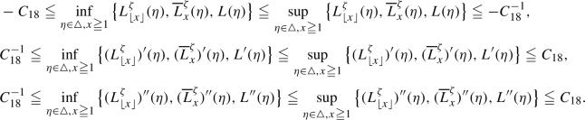
 , such that the following inequalities hold
Proof
(a) Due to the convexity of the exponential function we have \(\big |\frac{e^{h x}-1}{h}\big |\leqq xe^{hx}\vee 1\) for all \(x\geqq 0\) and \(h\in \mathbb {R}\). If we choose \(h_0:=\frac{|\eta |}{2}\), then since \(\zeta \leqq 0\), we have that for all \(|h|\leqq h_0,\)
Due to \(H_ye^{\eta H_y}\leqq \frac{1}{|\eta |}\) for all \(H_y\geqq 0\) and \(\eta <0,\) as well as \(\lim _{h\rightarrow 0}\frac{e^{hH_y}-1}{h}=H_ye^{hH_y}\) for all \(H_y\geqq 0\), dominated convergence yields for all \(\eta <0\) that
Then (A.1) is a consequence of the chain rule and the fact that the expectation on the left-hand side in (A.8) is positive. Then (A.2) follows from linearity of the derivative. To show (A.3), we have to apply dominated convergence once more. This time, we additionally need that the expectation on the left-hand side in (A.8) for \(x=1\) is strictly bounded from below by the constant \(E_1[e^{-(\texttt {es}-\texttt {ei}-\eta )H_0}]=e^{-\sqrt{2(\texttt {es}-\texttt {ei}-\eta )}}>0\) due to (BDD) and [4, (2.0.1), p. 204]. Using the mean value theorem and (A.7) entail the existence of \(c_1>0\) such that
Using (A.1) for \(x=1\) and dominated convergence, we arrive at (A.3).
By induction and similar arguments as above, it follows that for all \(n\in \mathbb {N}\), the function \((-\infty ,0)\ni \eta \mapsto E_x\big [(H_{y})^n e^{\int _0^{H_{y}}(\zeta (B_r)+\eta )\textrm{d}r} \big ]\) is positive \(\mathbb {P}\)-a.s. and differentiable. Due to (BDD), one can interchange expectation and differentiation in \(\eta ,\) yielding (A.4) and (A.5). The first equality in (A.6) is then again a consequence of dominated convergence. The strict inequalities in (A.4) and (A.6) are due to the fact that under \(P_1,\) and thus also \(\mathbb {P}\)-a.s. under \(P_1^{\zeta ,\eta }\), the random variable \(H_0\) is non-degenerate.
To show (b), observe that the function \(\zeta \mapsto E_x\big [e^{\int _0^{H_{\lceil x\rceil -1}}(\zeta (B_s)+\eta )\textrm{d}s}\big ]\) is nondecreasing. Consequently, using the notation \(\triangle =[\eta _*,\eta ^*]\), we have
where we used [4, (2.0.1), p. 204] for the second inequality and last equality. Due to the inequality \(e^{-xy}x\leqq \frac{2}{y}e^{-xy/2}\) for all \(x\geqq 0\) and \(y>0\), these estimates can be used to derive similar bounds for \(E_x\big [ e^{\int _0^{H_{\lceil x\rceil -1}}(\zeta (B_r)+\eta )\textrm{d}r}H_{\lceil x\rceil -1}^k \big ]\), \(k=1,2\). Thus, estimating the numerator and the denominator of the corresponding expressions in (A.1) to (A.6), we can conclude.
1.2 Exponential mixing
Lemma A.2
Let \(\mathcal {F}^k\) be as defined in (MIX), i.e. \(\mathcal {F}^k=\sigma (\xi (x):x\geqq k)\), and let \(\triangle \subset (-\infty ,0)\) be a compact interval. Then there exists a constant \(C_\triangle >0\) such that \(\mathbb {P}\)-a.s., for all \(i,j\in \mathbb {Z}\) with \(i< j\), and all \(\eta \in \triangle ,\)
as well as
Proof
By translation invariance, it is enough to prove (A.9) for \(i=0\) and \(j\geqq 2\) (the case \(j=1\) follows immediately from the uniform boundedness of \(L^\zeta _0\) and L on \(\triangle \) due to Lemma A.1). To show (A.9), let \(\eta \in \triangle \) and write \(L_0^\zeta (\eta )=\ln (A+B)\) with
and
Then \(A\leqq E_0[e^{H_{-1}\eta }] \leqq c_{\triangle ,1}<1,\) and, using (2.3), at the same time we have
To bound B, we condition on \(H_{-1}\) to happen before or after time j and use the reflection principle for Brownian motion and the tail estimate from [6, Lemma 1.1] to infer for all \(j\geqq 2\)
As \(\ln (1+x)\leqq x,\) the above implies that for all \(j\geqq 2\)
Since \(L_0^\zeta \) is continuous on \(\triangle \), the latter display \(\mathbb {P}\)-a.s. holds uniformly for all \(\eta \in \triangle .\) Now \(\ln (A)\) is \(\mathcal {F}_{\lceil j/2\rceil }\)-measurable and bounded, so by (MIX)
The proof of (A.11) is similar. Indeed, using the same notation we have \((L_0^\zeta )'=\frac{A'}{A+B}+ \frac{B'}{A+B}\). Then by \(A+B\geqq c_{\triangle ,2}\) and \(e^{\eta H_{-1}}H_{-1}\leqq \frac{2}{|\eta |}e^{\eta H_{-1}/2}\), we can use above calculation to conclude that \(\frac{B'}{A+B}\) decays exponentially to 0 as \(j\rightarrow \infty \). Further, \(\frac{A'}{A}-\frac{BA'}{A(A+B)}= \frac{A'}{A+B}\leqq \frac{A'}{A}\), \(F_{\lceil j/2\rceil }\)-measurability of \(\frac{A'}{A}\) and above estimates give a similar bound as in (A.13) for \((L_0^\zeta )'(\eta )\) and \(L'(\eta )\) instead of \((L_0^\zeta )(\eta )\) and \(L(\eta )\). Finally, (A.10) and (A.12) follow by the same arguments as (A.9) and (A.11).
1.3 Properties of the Lyapunov exponent
Proposition A.3
Assume (BDD) and (STAT) and let \(u^{(x,\delta )}\) be a solution to (PAM) with initial condition \(\mathbb {1}_{[x-\delta ,x+\delta ]}\). Then the limit \(\Lambda (v):=\lim _{t\rightarrow \infty } \frac{1}{t} \ln u^{(x,\delta )} (t,vt)\), \(v\in \mathbb {R}\), exists \(\mathbb {P}\)-a.s., is non-random and independent of \(x\in \mathbb {R}\) and \(\delta >0\). The function \([0,\infty )\ni v\mapsto \Lambda (v)\) is concave, \(\Lambda (0)=\texttt {es}\) and \(\lim _{v\rightarrow \infty } \frac{\Lambda (v)}{v}=-\infty \). In particular, there exists a unique \(v_0>0\) such that \(\Lambda (v_0)=0\).
Proof
Let \(x=0\), \(\lambda \in (0,1)\) and \(v_1,v_2\in \mathbb {R}\), and set \(v:=\lambda v_1 + (1-\lambda ) v_2\) and \(A:=[(1-\lambda )v_2t-\delta ,(1-\lambda )v_2t + \delta ]\). By (1.12), the solution to (PAM), admits the Feynman–Kac representation \(u^{(x,\delta )}(t,vt)=E_{vt}\big [ e^{\int _0^t \xi (B_s)\textrm{d}s}; B_t\in [x-\delta ,x+\delta ] \big ]\). Then by the Markov property, for all \(y\in [vt-\delta ,vt+\delta ]\) we have
Defining \(\overline{\mu }^{\delta }_{s,t}(v):= \inf _{y\in [vt-\delta ,vt+\delta ]} \ln E_y\big [ e^{\int _0^{t-s}\xi (B_r)\textrm{d}r}; B_{t-s}\in [vs-\delta ,vs+\delta ] \big ]\), \(s<t\), by the same argument as in the last display one can see that \(\overline{\mu }^{\delta }_{s,t}(v)\geqq \overline{\mu }^{\delta }_{s,u}(v) + \overline{\mu }^{\delta }_{u,t}(v)\) for all \(s<u<t\). Furthermore for the h-lateral shift \(\theta _h\) on \(\xi \) (i.e. \(\xi (\cdot )\circ \theta _h=\xi (\cdot +h)\)) we have \(\overline{\mu }^{\delta }_{s,t}(v)\circ \theta _h=\overline{\mu }^{\delta }_{s+\frac{h}{v},t+\frac{h}{v}}(v)\) for every \(h\in \mathbb {R}\), all \(v\ne 0\) and \(s<t\), and by (BDD) and a simple Gaussian computation there exists \(K_{\delta ,v} \in (0,\infty )\) such that \(\overline{\mu }^{\delta }_{0,t}(v)\geqq -K_{\delta ,v}\cdot t\) for all \(t\geqq 1\). By (BDD) we also have \(\overline{\mu }_{0,t}^\delta (v)\leqq \texttt {es}\cdot t\) and thus \(\overline{\mu }_{0,t}^\delta (v)\in L^1\) for all \(t>0\). Thus, Kingman’s subadditive ergodic theorem [23] implies that the limit \(\Lambda ^{\delta }(v):=\lim _{t\rightarrow \infty }\frac{1}{t}\overline{\mu }^{\delta }_{0,t}(v)\) exists \(\mathbb {P}\)-a.s. Furthermore, by (MIX), \(\xi \) is mixing and thus ergodic, so the \(\Lambda ^\delta (v)\) is non-random. By standard estimates, the limit is independent of \(\delta >0\) and \(x\in \mathbb {R}\).
To show the concavity of \(v\mapsto \Lambda (v)\), for \(v_1,v_2 \geqq 0\) and dividing by t, the left-hand side of (A.14) converges \(\mathbb {P}\)-a.s. to \(\Lambda (\lambda v_1 + (1-\lambda ) v_2)\), while the second term on the right-hand side of (A.14) converges \(\mathbb {P}\)-a.s. to \((1-\lambda )\Lambda (v_2)\). Dividing by t and using (STAT), the first term on the right-hand side of (A.14) converges in distribution to the constant \(\lambda \Lambda (v_1)\), proving the concavity of \(v\mapsto \Lambda (v)\).
By [14, Theorem 7.5.2] we have \(\lim _{t\rightarrow \infty }\frac{1}{t} \ln u^{\mathbb {1}_{(-\delta ,\delta )}}(t,0) =\texttt {es}\), independent of \(\delta >0\), giving \(\Lambda (0)=\texttt {es}\). Due to (BDD) and a standard Gaussian computation we have \(\lim _{v\rightarrow \infty }\frac{\Lambda (v)}{v}=-\infty \). This, together with \(\Lambda (0)=\texttt {es}>0\) and the concavity of \(v\mapsto \Lambda (v),\) implies the existence of a unique \(v_0>0\), such that \(\Lambda (v_0)=0\).
1.4 A Hoeffding-type inequality for dependent random variables
Lemma A.4
([34, Theorem 2.4]) Let \((X_i)_{i\in \mathbb {Z}}\) be a sequence of real-valued bounded random variables, \(\widetilde{\mathcal {F}}_i:=\sigma (X_j:j\leqq i)\), \(S_n:=\sum _{i=1}^{n}X_i,\) and let \((m_1,\ldots ,m_n)\) be an n-tuple of positive reals such that for all \(i\in \{1,\ldots ,n\},\)
with the convention \(\sum _{k=i+1}^i\mathbb {E}[X_k|\widetilde{\mathcal {F}}_i]=0\). Then for every \(x>0,\)
Rearranging the quantities in the above result, we arrive at the following corollary which we primarily pronounce explicitly since its formulation tailor-made for our purposes.
Corollary A.5
Let \((Y_i)_{i\in \mathbb {Z}}\) be a sequence of real-valued bounded random variables, \(\widetilde{\mathcal {F}}^k:=\sigma (Y_j:j\geqq k),\) and let \((m_1,\ldots ,m_{n})\) be an n-tuple of positive real numbers such that for all \(i\in \{1,\ldots ,n\},\)
with the convention \(\sum _{k=i}^{i-1}\mathbb {E}[Y_k|\widetilde{\mathcal {F}}^i]=0\). Then for every \(x>0,\)
Recall that \(u^{u_0}\) denotes the solution to (PAM) with initial condition \(u_0\).
Lemma A.6
For all \(x\in \mathbb {R}\) and \(0\leqq s\leqq t\) we have \( u^{\mathbb {1}_{(-\infty ,0]}}(s,x) \leqq 2u^{\mathbb {1}_{(-\infty ,0]}}(t,x). \)
Proof
By the Feynman–Kac formula, \(\xi \geqq 0\) and the Markov property at time s we have
Lemma A.7
Let \(N_{s,u,t}^\mathcal {L}\) be as in (4.1). Then there exists \(c>0\) such that \(\mathbb {P}\)-a.s.
Proof
Write \(A_{y,z,t}:=\big \{H_k + y \geqq z+t - T_k - 5\chi _1(\overline{m}(t))\ \forall k\in \{1,\ldots ,\lfloor \overline{m}(t)\rfloor \}\big \}\) and \(p(r):=\inf _{y\leqq 0}P_y(B_r\leqq 0)=\frac{1}{2}\). Then by the Feynman–Kac formula
with \(c:= \frac{1}{2}P_x(H_{\lfloor x\rfloor }\leqq 1)\).
The next result is an inequality of Harnack-type flavor for the solution to (PAM).
Lemma A.8
There exists a constant  such that \(\mathbb {P}\)-a.s. for all \(y\in \mathbb {R}\), \(t\geqq 1\) and all \(u_0\in \mathcal {I}_{\text {PAM}}\) we have

Proof
For \(x\in \mathbb {R}\) and \(t>0\) let \(f_{t,x}\) be the probability density of a Brownian motion at time t, starting in x. Let us first show that for all \(y,z\in \mathbb {R}\) we have
Indeed, using \(f_{t,y}(z)=\frac{1}{\sqrt{2\pi t}}e^{-\frac{(z-y)^2}{2t}}\), (A.17) follows from
The Feynman–Kac formula in combination with the Markov property applied at time 1 now supplies us with
where in the second inequality we used (A.17). Then (A.16) follows choosing  .
.
1.5 Proof of the McKean representation
Proof of Proposition 2.1
We start with considering \(w_0\) continuous and \(w_0(x)\in [0,1]\) for all \(x\in \mathbb {R}\). Define \(u:=1-w\) and \(u_0:=1-w_0\). Then by [21, Remark 4.4.4] (providing the existence of a \(C^{1,2}\)-solution to (PAM)) and [21, Corollary 4.4.5] (Feynman–Kac representation), the function \(u^{(1)}(t,x)=E_x\big [ e^{-\int _0^t\xi (B_r)\textrm{d}r} u_0(B_t) \big ]\) is a classical solution to \(u^{(1)}_t(t,x)=\frac{1}{2}\Delta u^{(1)}(t,x) - \xi (x)u^{(1)}(t,x)\) and we have \(u^{(1)}(0,x)=u_0(x)\). Furthermore, by the same argument, for all \(s<t\) and \(k\in \mathbb {N}\) fixed, the function
is a classical solution to \(u^{(2)}_t(t,x;s,k)=\frac{1}{2}\Delta u^{(2)}(t,x;s,k) - \xi (x)u^{(2)}(t,x;s,k)\). By dominated convergence, taking advantage of the uniform continuity of the first and second order derivatives, for every fixed \(t'\leqq t\), we can interchange limits to obtain the identities
Conditioning on the first splitting time of the initial particle and on the number of children that are born, we have
where we used the Markov property of the process \((B_t)_{t\geqq 0}\). We deduce that for \(h\ne 0,\)
Invoking once again the arguments from the beginning of the proof, as h tends to zero, the first summand converges to \(\frac{1}{2}\Delta u^{(1)}(t,x) - \xi (x)u^{(1)}(t,x)\) and by dominated convergence, the second summand converges to \(\xi (x)\sum _k p_k u(t,x)^k\). For the third term, we mention that the integrand is uniformly bounded since \(u^{(2)}_t\) is continuous. Again, due to dominated convergence and (A.18), the latter term converges to
All in all, combining these observations we arrive at
which is equivalent w being a solution to (F-KPP). Thus we have shown the claim for continuous \(w_0\). By Remark 1.2, for \(w_0\in \mathcal {I}_{\text {F-KPP}}\) the result follows by approximation.
1.6 Existence and monotonicity of solutions
We start with an existence result for generalized and also classical solutions.
Proposition A.9
([14, Theorem 7.4.1]) Let \(w_0\) be measurable, non-negative and bounded, and let F fulfill (SC). Then \(\mathbb {P}\)-a.s. there exists a unique, bounded generalized solution \(w\in C\big ( (0,\infty )\times \mathbb {R}\big )\) to (F-KPP), which satisfies \(0\leqq w(t,x)\leqq 1\vee \sup _x w_0(x)\) for all \((t,x)\in [0,\infty )\times \mathbb {R}\). If additionally \(w_0\) is continuous and \(x\mapsto \xi (x,\omega )\) is Hölder continuous for \(\mathbb {P}\)-a.a. \(\omega \in \Omega \), then \(\mathbb {P}\)-a.s. the generalized solution w is a classical one, i.e. \(w\in C^{1,2}\big ((0,\infty )\times \mathbb {R}\big )\cap C\big ([0,\infty )\times \mathbb {R}\big )\) and w solves (F-KPP).
For the next lemma, we introduce the differential operator
where G is uniformly Lipschitz-continuous in w, i.e., there exists a constant \(\alpha >0\), such that
The next lemma is in the spirit of [1, Proposition 2.1].
Lemma A.10
Let \(T>0\), \(Q:=(0,T)\times \mathbb {R}\) and G be such that (A.19) holds. Let \(w^{(1)}\) and \(w^{(2)}\) be non-negative and bounded functions on \(\overline{Q}\), such that for \(i\in \{1,2\}\), \(w^{(i)}_x\) and \(w^{(i)}_{xx}\) are continuous on Q, and such that \(w^{(i)}_t\) exists in Q. If \(\mathcal {L}_{G}w^{(1)} \leqq \mathcal {L}_{G}w^{(2)}\) on Q and \(0\leqq w^{(1)}(0,x)\leqq w^{(2)}(0,x)\) for all \(x\in \mathbb {R}\), then also \(w^{(1)} \leqq w^{(2)}\) on Q.
Proof
From the assumptions we infer that
Then, recalling (A.19) and letting
we get
Now the the first factor on the right-hand side is negative and bounded. Applying the maximum principle [25, Theorem 8.1.4] to \(-v\) then implies that \(v \geqq 0\) on Q and we can conclude.
As an important application we get that the solution w to \(\mathcal {L}_Gw=0\) is monotone in G and in the initial condition.
Corollary A.11
Let \(T>0\), \(Q:=(0,T)\times \mathbb {R}\), and let \(G_1\) and \(G_2\) fulfill \({G_1}\leqq {G_2}\) on \(\mathbb {R}\times [0,\infty ).\) Furthermore, assume that \(G_2\) satisfies (A.19). In addition, let \(w^{(1)}\) and \(w^{(2)}\) be non-negative and bounded functions on \(\overline{Q}\), such that for \(i\in \{1,2\}\), \(w^{(i)}_x\) and \(w^{(i)}_{xx}\) are continuous on Q and \(w^{(i)}_t\) exist on Q. If \(\mathcal {L}_{G_1}w^{(1)} = \mathcal {L}_{G_2}w^{(2)}\) and \(w^{(1)}(0,\cdot )\leqq w^{(2)}(0,\cdot )\) on \(x\in \mathbb {R}\), then we have \(w^{(1)} \leqq w^{(2)}\) on Q.
Proof
Since the function \(w^{(2)}\) is non-negative, we have \(\mathcal {L}_{G_2}w^{(2)}=\mathcal {L}_{G_1}w^{(1)}\geqq \mathcal {L}_{G_2}w^{(1)}\). Then by Lemma A.10, we have \(w^{(1)}(t,x)\leqq w^{(2)}(t,x)\) for all \((t,x)\in Q\).
Corollary A.12
Let G fulfill (A.19) and \(G(x,0)=G(x,1)=0\) for all \(x\in \mathbb {R}\). Let w be a solution to \(\mathcal {L}_Gw=0\) with \(0\leqq w(0,x)\leqq 1\). Then \(0 \leqq w(t,x) \leqq 1\) for all \((t,x)\in [0,\infty )\times \mathbb {R}\).
Proof
The functions \(w^{(1)}(t,x)=0\) and \(w^{(2)}(t,x)=1\) are solutions to \(\mathcal {L}w^{(1)}=\mathcal {L}w^{(2)}=0\) and \(w^{(1)}(0,x)\leqq w(0,x)\leqq w^{(2)}(0,x)\). The claim then follows from Lemma A.10.
Rights and permissions
Open Access This article is licensed under a Creative Commons Attribution 4.0 International License, which permits use, sharing, adaptation, distribution and reproduction in any medium or format, as long as you give appropriate credit to the original author(s) and the source, provide a link to the Creative Commons licence, and indicate if changes were made. The images or other third party material in this article are included in the article’s Creative Commons licence, unless indicated otherwise in a credit line to the material. If material is not included in the article’s Creative Commons licence and your intended use is not permitted by statutory regulation or exceeds the permitted use, you will need to obtain permission directly from the copyright holder. To view a copy of this licence, visit http://creativecommons.org/licenses/by/4.0/.
About this article

Cite this article
Drewitz, A., Schmitz, L. Invariance Principles and Log-Distance of F-KPP Fronts in a Random Medium. Arch Rational Mech Anal 246, 877–955 (2022). https://doi.org/10.1007/s00205-022-01824-x
Received:
Accepted:
Published:
Issue Date:
DOI: https://doi.org/10.1007/s00205-022-01824-x