
Abstract
We study the regularity of the flow \({\varvec{X}}(t,y)\), which represents (in the sense of Smirnov or as regular Lagrangian flow of Ambrosio) a solution \(\rho \in L^\infty ({\mathbb {R}}^{d+1})\) of the continuity equation
with \({\varvec{b}}\in L^1_t {{\,\textrm{BV}\,}}_x\). We prove that \({\varvec{X}}\) is differentiable in measure in the sense of Ambrosio–Malý, that is
where the derivative W(t, y) is a BV function satisfying the ODE
where \((D{\varvec{b}})_y(\textrm{d}t)\) is the disintegration of the measure \(\int D {\varvec{b}}(t,\cdot ) \, \textrm{d}t\) with respect to the partition given by the trajectories \({\varvec{X}}(t, y)\) and the Jacobian J(t, y) solves
The proof of this regularity result is based on the theory of Lagrangian representations and proper sets introduced by Bianchini and Bonicatto in [16], on the construction of explicit approximate tubular neighborhoods of trajectories, and on estimates that take into account the local structure of the derivative of a \({{\,\textrm{BV}\,}}\) vector field.
1 Introduction
We consider a vector field \({\varvec{b}}: {\mathbb {R}}\times {\mathbb {R}}^d \mapsto {\mathbb {R}}^d\) of class \(L^1_t {{\,\textrm{BV}\,}}_x\), and a solution \(\rho \in C([0,T],L^\infty _{\textrm{w}}({\mathbb {R}}^d))\) to the continuity equation
We assume that \({\varvec{b}}\) and \(\rho \) are compactly supported. From the results of [16], it follows that \(\rho \) has a unique representation is terms of characteristics, that is absolutely continuous solutions to the ODE
More precisely, there exists a unique flow \({\varvec{X}}: [0,T] \times {\mathbb {R}}^d \rightarrow {\mathbb {R}}^d\), defined for \(\rho (0,\cdot ) {\mathcal {L}}^d\)-almost everywhere \(y \in {\mathbb {R}}^d\), such that
which means that, for every test function \(\varphi \in C^\infty _c((0,T)\times {\mathbb {R}}^d)\),
For the precise statement, see Theorem 3.5 of Section 3.2. The appropriate notion of flow for ODEs driven by rough (non-Lipschitz continuous) vector fields, introduced in the seminal papers [8, 40], is the one of regular Lagrangian flow, which consists of a measurable selection of characteristics such that \({\varvec{X}}(t,\cdot )_\sharp {\mathcal {L}}^d \leqq C {\mathcal {L}}^d\) holds (see, for example, [9, 10] for further information).
The main result of this paper is the differentiability in measure of the flow \({\varvec{X}}\) (in the sense of Ambrosio–Malý, see [13]). Let \((D{\varvec{b}})_y\) be the rescaled conditional probabilities associated with the disintegration of \(D{\varvec{b}}\) along the trajectories of \({\varvec{X}}\); that is, if
where F is a \(\sigma \)-compact set where \(\rho (0, \cdot )\) is concentrated, then (up to a negligible \((\rho (0,\cdot ) {\mathcal {L}}^d)\)-set)
or, equivalently, for every test function \(\varphi \in C_c({\mathbb {R}}^+ \times {\mathbb {R}}^d)\),
Similarly, for the divergence \({{\,\textrm{div}\,}}{\varvec{b}}\), we can write
Our main theorem is as follows:
Theorem 1.1
(Differentiability in measure of the flow associated to a BV vector field) The flow \({\varvec{X}}:[0,T]\times {\mathbb {R}}^d \rightarrow {\mathbb {R}}^d\) is differentiable in measure at any time \(T>0\): that is, for every \({\varepsilon }>0\), we have
for some matrix valued function W(T, y). Moreover, the matrix W(t, y) satisfies the ODE
and the Jacobian J(t, y) satisfies the ODE
In the statement \(W(t-,y)\), \(J(t-,y)\) are the left limits of \(W(\cdot ,y)\), \(J(\cdot ,y)\), whose existence follows from the fact that they solve their respective ODE with measure right-hand side and then are BV functions of time; we also notice that, in general, \(W(\cdot ,y)\) and \(J(\cdot ,y)\) are discontinuous due to the singular measure \((D{\varvec{b}})_y\). We remark that the convergence in measure expressed by formula (1.2) can be written equivalently as
1.1 Uniqueness and regularity of the flow associated to a rough velocity field
The study of the well-posedness of transport equations driven by rough velocity fields started with the pioneering paper [40], where DiPerna and Lions introduced the notion of renormalized solution and proved existence and uniqueness for (1.1) in the case of Sobolev \(W^{1,p}\) vector fields (with \(p \in [1,\infty ]\)) with bounded divergence (or divergence in a suitable \(L^p\) space). Ambrosio extended the theory to \({{\,\textrm{BV}\,}}\) vector fields with bounded divergence in [8] (see also [32, 48]). More recently, Bianchini and Bonicatto proved a uniqueness result in the more general case of nearly incompressible \({{\,\textrm{BV}\,}}\) vector fields (see [16]), obtaining, as a consequence, a positive answer to Bressan’s compactness conjecture (see [27]). We refer also to the more recent [17] for a variation of the strategy in [27].
A locally integrable vector field is called nearly incompressible if there exists a solution \(C^{-1} \leqq \rho (t,x) \leqq C\) for \({\mathcal {L}}^{d-1}\)-almost everywhere \((t,x) \in (0,T) \times {\mathbb {R}}^d\) to the continuity equation (1.1); such assumption is implied by the stronger condition \(\div {\varvec{b}}\in L^\infty \). We refer the reader to [9, 10, 37] and the references therein for a more comprehensive overview of this area of research.
In case \({\varvec{b}}\in L^1_t W^{1,1}_x\) and divergence-free (plus some growth assumptions), in [46], Le Bris and Lions proved that, if \({\varvec{X}}(t,y)\) is the unique regular Lagrangian flow generated by \({\varvec{b}}\), then there exists a limit for the incremental ratio
and W(t, y, r) is a renormalized solution to
or, equivalently, any renormalized solution to
is given by
In [13], Ambrosio and Malý proved that \(W(t,y,r) = W(t,y) r\), and compared this differentiability in measure to other notions of differentiability. As it turns out (see [13, Section 5]), this property is much weaker than approximate differentiability (see [11, Section 3.6]).
Approximate differentiability of regular Lagrangian flows generated by \(W^{1,p}\) vector fields, with \(p > 1\), was first obtained by Ambrosio, Lecumberry and Maniglia in [12]. In [33], Crippa and De Lellis improved this result by proving a quantitative estimate of Lusin–Lipschitz type for the flow generated by a \(L^1_tW^{1,p}_x\) vector field with bounded divergence, with \(p>1\): for every \({\varepsilon }\), one can remove a set of measure \({\varepsilon }\) and \({\varvec{X}}(t=T)\) on the remaining set coincides with a Lipschitz continuous function having Lipschitz constant \(e^{C/{\varepsilon }}\). Their approach is based on a priori estimates for a functional measuring a “logarithmic distance” between two flows associated to the same vector field (see also [21, 24, 34, 44, 45, 49, 53,54,55, 57, 58] for related results that rely on this strategy). However, as noted in [31], this approach cannot be used to prove a regularity result for the flow associated to a \({{\,\textrm{BV}\,}}\) vector field.
A quantitative Lusin–Lipschitz regularity results for the flow \({\varvec{X}}\) associated to a vector field \({\varvec{b}}\) implies lower bounds on the mixing scale of passive scalars driven by \({\varvec{b}}\) through the transport equation (1.1) (see [56]). In particular, extending the result by Crippa and De Lellis to the case \(p=1\) would give a positive answer to the well-known Bressan’s mixing conjecture proposed in [28] (see also [5,6,7, 15, 29, 30, 35, 36, 41, 43, 47, 50, 51, 59, 62] for related results on both transport and advection-diffusion equations).
For the special case of bounded autonomous divergence-free vector fields \({\varvec{b}}\in {{\,\textrm{BV}\,}}({\mathbb {R}}^2; {\mathbb {R}}^2)\) with compact support, in [23], Bonicatto and Marconi proved a Lusin–Lipschitz regularity result and showed that the Lipschitz constant grows at most linearly in time. In this setting, the analysis is facilitated by the Hamiltonian structure of the vector fields (see [2,3,4, 18, 20, 22]).
In the present paper, we establish the differentiability in measure for a nearly incompressible vector field \({\varvec{b}}\in L^1_t {{\,\textrm{BV}\,}}_x\). Our approach is based on the localization of the problem (which relies on the theory of proper sets introduced in [16]): we exploit the local structure of the vector field \({\varvec{b}}\) to prove differentiability in measure locally; then, Theorem 1.1 is obtained by suitably combining the local estimates.
1.2 Notations
For an integer \(d \geqq 1\), the d-dimensional Euclidean real vector space is denoted by \({\mathbb {R}}^d\). We write the component of a d-dimensional point or vector as \(x = (x_1,\dots ,x_d)\); we also write \(x_{\not i,\not j,\dots }\) to denote the point obtained by removing the coordinate component \(i,j,\dots \) from x. The unit vector along the i-coordinate is \({\textbf{e}}_i\).
The d-dimensional ball in \({\mathbb {R}}^d\) of radius r centered at x is written as \(B^d_r(x)\). Given a curve \(t \mapsto \gamma (t) \in {\mathbb {R}}^d\), we write
The relative closure of the set A in the topological space B is denoted by \(\textrm{clos}(A, B)\); we also write \({\text {clos}} A\) when the ambient topological space is clear. Similarly, the interior of a set A is written as \({\text {int}} A\) or \(\textrm{int}(A, B)\). The boundary is denoted by \({\text {Fr}} A\) or \(\textrm{Fr}(A, B)\) or, sometimes, by the standard notation \(\partial A\). We write \(A \Subset B\) if \({\text {clos}} A\) is a compact set contained in B.
\({\mathbb {I}}\) is the identity matrix, the minimum between two quantities a, b is denoted by \(a \wedge b\), and the maximum by \(a \vee b\).
The d-dimensional Lebesgue measure is denoted by \({\mathcal {L}}^d\), and the k-dimensional Hausdorff measure by \({\mathcal {H}}^k\).
If X is a set and \({\mathscr {A}}\) is a \(\sigma \)-algebra on X, we will call \((X, {\mathscr {A}})\) a measure space. A measure \(\mu \) is concentrated on a set \(C \subset X\) if \(|\mu |(X {\setminus } C) = 0.\) Let \(\mu \) be a measure on \((X, {\mathscr {A}})\) and \(A \in {\mathscr {A}}\). We define the restriction \(\mu {\displaystyle \llcorner }_A\) of \(\mu \) to A as the measure on \({\mathscr {A}}\) given by \(\mu {\displaystyle \llcorner }_A(E):= \mu (A \cap E)\) for any \(E \subset {\mathscr {A}}\).
The \(\sigma \)-algebra generated by open sets is called Borel \(\sigma \)-algebra and will be denoted by \({\mathscr {B}}(X)\). Let X, Y be two metric spaces, \(\mu \) a measure on \((X, {\mathscr {B}}(X))\) and \(f:X \rightarrow Y\) a Borel function. We define the push-forward of \(\mu \) with respect to f as the measure on \((Y, {\mathscr {B}}(Y))\) given by \(f_\sharp \mu (B) := \mu (f^{-1}(B))\) for all \(B \in {\mathscr {B}}(Y)\). In particular, for a Borel map \(g:Y \rightarrow {\mathbb {R}}\) it holds that
The disintegration of a measure \(\mu \) with respect to a partition \(\{A_\alpha \}_\alpha \) is written as
where f is the partition function, that is \(f^{-1}(\alpha ) = A_\alpha \) (see [42, Section 452]).
The Lebesgue spaces \(L^p(X,\mu ;Y)\) are defined in the usual way; if \(X={\mathbb {R}}^d\) and \(\mu = {\mathcal {L}}^d\), we just write \(L^p({\mathbb {R}}^d; Y)\); if, moreover, \(Y = {\mathbb {R}}\), we write \(L^p({\mathbb {R}}^d)\). We use the standard notation for Sobolev spaces. We denote by \([{\mathcal {M}}_{loc}(X)]^m\) and by \([{\mathcal {M}}(X)]^m\), respectively, the space of \({\mathbb {R}}^m\)-valued Radon measures and the space of \({\mathbb {R}}^m\)-valued finite Radon measures. The space \([{\mathcal {M}}(X)]^m\) is a Banach space with the norm \(\Vert \mu \Vert _{{\mathcal {M}}} := |\mu |(X)\), where \(|\mu |\) is the total variation of the measure \(\mu \). In the case \(m=1\), we denote the set of signed Radon measures, positive Radon measures, and finite Radon measures by \({\mathcal {M}}(X)\), \({\mathcal {M}}^+(X)\), and \({\mathcal {M}}_b(X)\) respectively (see [11, Chapter 1]).
We say that \({\varvec{b}}\in L^1(\Omega ; {\mathbb {R}}^m)\) has bounded variation in \(\Omega \), and we write \({\varvec{b}}\in {{\,\textrm{BV}\,}}(\Omega ; {\mathbb {R}}^m)\) if \(D{\varvec{b}}\) is representable by a \({\mathbb {R}}^{m\times d}\)-valued measure with finite total variation in \(\Omega \). Endowed with the norm \(\Vert {\varvec{b}}\Vert _{{{\,\textrm{BV}\,}}(\Omega )} = \int _{\Omega } |u| \, \textrm{d}x + |D{\varvec{b}}|(\Omega ) = \Vert {\varvec{b}}\Vert _{L^1(\Omega )} + \Vert D{\varvec{b}}\Vert _{{\mathcal {M}}(\Omega )}\), the space \({{\,\textrm{BV}\,}}(\Omega ; {\mathbb {R}}^m)\) is a Banach space (see [11, Chapter 3]). We will use the notation
for the continuous, jump, absolutely continuous, and Cantor parts of \(D{\varvec{b}}\).
Given a Banach space X, by \(L^p([0,T];X)\) we denote the Lebesgue-Bochner space of strongly measurable maps \(f:[0,T]\rightarrow X\) with \(\Vert f\Vert _{L^p([0,T];X)}^p:=\int _0^T \Vert f\Vert ^p_X \, \textrm{d}t<\infty \). For the sake of brevity, we often write \(L^p_tX_x\) to indicate \(L^p([0,T];X)\). We add the subscript loc to denote properties which holds locally.
For a vector field \({\varvec{b}}:{\mathbb {R}}^{d+1} \rightarrow {\mathbb {R}}^d\), sometimes we also use the notation \({\varvec{b}}(t): {\mathbb {R}}^d \rightarrow {\mathbb {R}}^d\); moreover, for the vector field \({\varvec{b}}\in L^1_t {{\,\textrm{BV}\,}}_x\), we write \(D{\varvec{b}}\) to denote the measure
while \(D{\varvec{b}}(t)\) denotes the space derivative of \({\varvec{b}}\) at time t. Similar notations are used for \(|D{\varvec{b}}|\).
We write \(f(x\pm )\) to denote the right/left limit of f in x (when such limit exists, for example in case \(f \in {{\,\textrm{BV}\,}}({\mathbb {R}})\), see [11]).
If A is a Borel set of positive measure, we write the average integral of \(f \in L^1(\mu )\) as

We say that \(\gamma : (t^-,t^+) \mapsto {\mathbb {R}}^d\) is a characteristic of the vector field \({\varvec{b}}: {\mathbb {R}}\times {\mathbb {R}}^d \rightarrow {\mathbb {R}}^d\) if it is an absolutely continuous function such that
If the ODE above generates a flow, we use the notation \({\varvec{X}}(t,s,y)\) for the solution to (1.5) with initial data y at time s. The graph of \({\varvec{X}}\) in a time interval (s, t) is denoted by \({\varvec{X}}((t,s),y)\), and when we restrict the curve to some open set \(\Omega \) we will use the notation \({\varvec{X}}(t,t^-(y),y)\), with \(y \in \partial \Omega \) and \(X(t^-(y),t^-(y),y) = y\); the exit time is denoted by \(t^+(y)\). For the sets (perturbed proper sets) that we are considering in this paper, all quantities (entering/exiting time \(t^\pm (y)\) with respect to the regular Lagrangian flow \({\varvec{X}}\)) are well defined (cf. the discussion in [16]).
If K is a compact set of initial data, we use the notation \({\mathcal {K}}\) to denote the union of its trajectories,
2 Structure of the Paper
The proof of our main result is quite technical. In this section, we outline its structure and the reason of the technicalities. Moreover, we provide a sketch of the proof under the stronger assumption \({\varvec{b}}\in L^1_t W^{1,1}_x\) (which makes the argument much easier) and show where the difficulties for the \({{\,\textrm{BV}\,}}\) case lie.
In Section 3, we present some preliminary results that are needed in the proof of our main theorem. In Section 3.1, we collect some technical results on the existence of open sets \(\Omega \subset [0,T]\times {\mathbb {R}}^d\) with particularly nice properties for the vector field \((1,{\varvec{b}})\), the so-called proper sets, introduced in [16]. Roughly speaking, these are open sets where the problem can be meaningfully localized. Since the argument of the proof is based on the analysis of local properties of the vector field \({\varvec{b}}\), the tool of proper sets plays a fundamental role. The main results are Lemma 3.2, which states that there are sufficiently many of them, and Theorem 3.4, which allows us to perturb them so that there are finitely many “time-flat” boundary regions where the majority of the flow of \((1,{\varvec{b}})\) is entering or leaving. The motivation for this construction is that it is much easier to state the differentiability of the flow \({\varvec{X}}\) when it is parameterized by its crossing point y on a flat surface; we acknowledge that it is also possible to avoid this, but we decided to use perturbed proper sets since this tool has already been established in the literature (see [16]).
Section 3.2 deals with Smirnov’s decomposition of \((1,{\varvec{b}})\), which is stated in Theorem 3.5: that is, thanks to the superposition principle, which has been established by Ambrosio in [8] (see also [60] in the context of a general normal 1-current and [61]), every non-negative (possibly measure-valued) solution to the PDE (1.1) can be written as a superposition of solutions obtained via propagation along the characteristics of \({\varvec{b}}\) (such representation is also called a Lagrangian representation, see [16, Section 5]). Theorem 3.5 is used to construct \(L^\infty \) solutions \(\rho \) satisfying (1.1) by considering the curves \(\gamma _{\mathfrak {a}}\) of the decomposition which start from 0 and arrive to T, and such that the Jacobian of the transformation \(\gamma _{\mathfrak {a}}(0) \mapsto \gamma _{\mathfrak {a}}(t)\) is uniformly bounded.
In Section 3.3, we observe that our main theorem also gives the differentiability in measure of the Smirnov decomposition of \((1,{\varvec{b}})\): by a countable partition of the set of curves \(\{\gamma _a\}_{\mathfrak {a}}\) used in the Smirnov decomposition, one can find countably many \(L^\infty \)-solutions \(\rho _i {\mathcal {L}}^{d+1}\), \(i \in {\mathbb {N}}\), of (1.1) defined for \(t \in (t^-_i,t^+_i)\) such that
and apply Theorem 1.1 to this set of trajectories. Finally, in this section, we also select the curves for which we address the differentiability in order to have a uniform control of the rescaled conditional probabilities \((D{\varvec{b}})_y\) and \(({{\,\textrm{div}\,}}{\varvec{b}})_y\) and to have \(y \mapsto {\varvec{X}}(\cdot ,y)\) continuous in \(C^0\). The precise statement is in Proposition 3.6, which is an application of Lusin’s theorem.
2.1 Case \({\varvec{b}}\in L^1_t W^{1,1}_x\)
We sketch the proof of differentiability in measure for the case \({\varvec{b}}\in L^1_t W^{1,1}_x\). Under this assumption, we can directly estimate
where W(t, y) solves the ODE
Here we make use of the fact that the rescaled conditional probabilities \((D{\varvec{b}})_y\) are given by \(\nabla {\varvec{b}}(t,{\varvec{X}}(t,y)) J(t,y)\) due to the change of variable \((t,x) \mapsto (t,{\varvec{X}}(t,y))\) and Fubini’s theorem. We remark that, by Fubini’s theorem, we also have \(\nabla {\varvec{b}}(t,{\varvec{X}}(t,y)) \in L^1(0,T)\), so that the ODE (6.1) is well-defined.
Being that W(t, y)z is a Lipschitz continuous function in z and an absolutely continuous (a.c.) function in t, we can use the following estimate for Lipschitz semigroups (see [25, Lemma 4] or [26, Theorem 2.9], applied here as in Corollary A.2): for \(\rho (0,\cdot ) {\mathcal {L}}^d\)-almost everywhere \(y \in {\mathbb {R}}^d\), if \(t^+(y,rz) \in [0,T]\) is the exit time of the trajectory \({\varvec{X}}(t,y+rz)\) from the set
then
This estimate follows from integrating of the infinitesimal error at time \(t>0\)
along the trajectory, and multiplying it by the Lipschitz constant \(e^{\int _0^T |D{\varvec{b}}|(t,{\varvec{X}}(t,y)) \, \textrm{d}t}\) of the semigroup generated by (2.1). Since we are considering trajectories \(\{{\varvec{X}}(\cdot ,y)\}_{y \in K}\) such that
for some fixed M (this is part of the statement of Proposition 3.6, see discussion above), we have the exponential factor in (2.2) is bounded by \(e^M\) and the Jacobian is controlled by
and then, integrating for all \((y,z) \in K \times B^d_{1}(0)\), we obtain the bound

where \(C_d\) is a dimensional constant and
The last integral in (2.5) converges to 0 due to the continuity of translations in \(L^1\), and this shows that the set of trajectories starting in \(B^d_r(y)\) and exiting the cylinder \({\varvec{X}}(t,y) + B^d_{R}(0)\) with
can be made arbitrarily small and, for the remaining ones, the double integral converges to 0: more precisely, since by (2.1) and (2.3) one has \(|W(t,y)| \leqq e^{M}\), then, by Chebyshev’s inequality,

This yields the convergence in measure.
2.2 Case \({\varvec{b}}\in L^1_t {{\,\textrm{BV}\,}}_x\).
The argument above also highlights what is the key difficulty of the \({{\,\textrm{BV}\,}}\) case: the dependence \({\mathbb {R}}^d \ni y \mapsto (D{\varvec{b}})_y \in {\mathcal {M}}({\mathbb {R}})\) is only weakly continuous, and then (2.5) gives only a bound in terms of the constant \(|D{\varvec{b}}|_y(0,T) \leqq M\), and the last integral of (2.5) does not converge to 0. The present paper deals precisely with how to remove this difficulty.
The following diagram represents a general scheme of the proof and outlines its various components as well as the relations among them:

The sections are almost independent from each other, and their arrangement in the paper could be altered. We first study the ODE (Section 4) to obtain some useful bounds on W(t, y), and then present the local-to-global argument (Section 5), in order to have a clear picture of the local estimates one has to prove. As one can imagine, the most complex part of the paper is the one concerning local estimates for the singular part \(D^\textrm{sing}{\varvec{b}}\).
In the remaining part of this introduction, we present a detailed description of these core sections. According to the notations of Section 1.2, we write \((t^-,t^+)\) for the interval of time a trajectory spends inside an open set \(\Omega \) (and \((t^-_i(y),t^+_i(y))\) if the trajectory is \({\varvec{X}}(t,y)\) and the open set is \(\Omega _i\)). When we are considering a single proper set \(\Omega \), trajectories are parameterized by their entrance point y, and are considered distinct after reentering. This is in accord with the property of proper sets that the restriction of a Lagrangian representation to a proper set is still a Lagrangian representation (see [16, Section 5]).
In Section 4, we study the ODE (1.3) for the Jacobian matrix W(t, y), that is
Since this is not the classical setting, we provide a constructive proof of the well-posedness theorem (Theorem 4.1) based on the convergence of an Euler scheme. An interesting observation (Remark 4.3) is that if we require the ODE for W to be time invertible, that is that \(W(T-t,y)\) satisfies
the rank-one property of the vector field is needed (see [1]). This remark could be used in the case of 2d-autonomous vector fields to have another proof of Alberti’s rank-one theorem, because in this case the well-posedness does not require rank-one (see [4]), although clearly there are much simpler proof of rank-one property in the literature (see, for example, [38, 39, 52]).
The core of the proof is in the next four sections: in order, first, we present the argument to prove the differentiability in measure if there exists a partition into perturbed proper sets where suitable properties are satisfied (Section 5), then these properties are proved for the a.c. part of the derivative (Section 6) and for the singular part (Section 7), and finally the partition is constructed (Section 8).
The local-to-global argument is in Section 5: we prove that the existence of a partition into (perturbed) proper sets where approximate local differentiability assumptions are satisfied implies a global result on differentiability in measure. In the beginning (page 18), the key assumptions on the partition into perturbed proper sets are stated, which can be explained as follows: apart from the smallness of a measure \(\mu _P\) controlling the total error (Assumption (1)) and the fact that the trajectories considered for the differentiability are sufficiently close (Assumptions (2) and (3)), the key assumption is that there exists an approximate flow \({\tilde{{\varvec{X}}}}(r,y;t,z)\) which approximates both the perturbation \({\varvec{X}}(t,y+z) - {\varvec{X}}(t,y)\), when the latter quantity has \({\mathbb {R}}^d\)-norm smaller than r, and also the derivative W(t, y)z (Assumptions (5) and (7)). Moreover, the approximate flow \({\tilde{{\varvec{X}}}}\) has a controlled growth, as in Assumption (6). The reason why we need to introduce this approximate flow \({\tilde{{\varvec{X}}}}\) is because \(y \mapsto (D{\varvec{b}})_y\) is only weakly continuous, as we explained before in Section 2.1, so we choose a flow \({\tilde{{\varvec{X}}}}\) that solves an ODE for which the convergence of \(\dot{{\tilde{{\varvec{X}}}}}\) to \((D{\varvec{b}})_y\) is in mass and not in the weak sense (or, equivalently, their difference in norm is small). This comparison works only at the initial and final time (as shown also in Assumption (7), where the comparison is directly between \({\varvec{X}}(t,y+z) - {\varvec{X}}(t,y)\) and W(t, y)z). There are some additional technical assumptions, in particular that the estimates are valid only after removing some trajectories (Assumption (4)), which is also the reason why we obtain only differentiability in measure (instead of approximate differentiability).
The argument to pass from these local assumptions to a global differentiability result is presented in Proposition 5.1. First, we remove all trajectories which do not satisfy the previous estimates in some of the sets \(\Omega _i\) of the partition: these are controlled by the measure \(\mu _P\), which is assumed to be small (Step 1–3 of the proof). Second, we control the perturbations \({\varvec{X}}(t,y+z) - {\varvec{X}}(t,y)\) which do not remain close to 0 (that is \({\varvec{X}}(t,y+z)\) not close to \({\varvec{X}}(t,y)\)) for all \(t \in [0,T]\) (Step 5-11 of the proof): the idea here is that, in order to exit the ball \(B^d_R({\varvec{X}}(t,y))\), a trajectory has first to growth much more of the approximate flow \({\tilde{{\varvec{X}}}}(R,y;t,z)\), and a suitable choice of the initial distance r and of R yields a control on these runaway trajectories (similar to (2.6)). For the remaining ones, a suitable comparison with the linearized flow W(t, y)z holds. This yields the differentiability in measure (Step 12-13).
Sections 6 and 7 show that it is possible to construct proper sets where the local estimates required at the beginning of Section 5 are satisfied. The analysis of the absolutely continuous part is roughly the same as the one sketched in Section 2.1 for the \({\varvec{b}}\in L^1_tW^{1,1}_x\) case; as an additional error term, the mass of the singular part \(D^\textrm{sing}{\varvec{b}}\) inside the proper set also appears. The analysis of the singular part is instead the core of the paper, and requires many technical estimates. The first step is to consider a small neighborhood of a Lebesgue point of the singular part of the derivative (Section 7.1). This allows us to write \(D{\varvec{b}}\simeq {\bar{\xi }} \otimes {\bar{\eta }} |D{\varvec{b}}|\) (by Alberti’s rank-one theorem), and to use the latter measure to build an approximate vector field whose flow is \({\tilde{{\varvec{X}}}}\). The definition of the approximate vector field \({\tilde{{\varvec{b}}}}^H(r,y;t,w)\) is in Section 7.2, and its explicit expression is in formula (7.5), namely assuming \({\bar{\eta }} = {\textbf{e}}_1\) and \({\bar{\xi }} = {\bar{\xi }}_1 {\textbf{e}}_1 + {\bar{\xi }}_2 {\textbf{e}}_2\),
where
The choice of H follows the ideas of [8, 16]. The parameter H needs to be sufficiently large, while \(r \ll 1\) in order to be inside the neighborhood of the Lebesgue points of \(D^\textrm{sing}{\varvec{b}}\). How close \({\tilde{{\varvec{b}}}}^H\) is to \(D{\varvec{b}}\) is estimated in Proposition 7.1. The choice of \(\tilde{\varvec{b}}^H\) is based on the following considerations. First, the derivative depends essentially on first coordinate \(w_1\), so that \({\tilde{{\varvec{b}}}}^H\) depends only on the first coordinate. Secondly, the solution \({\tilde{{\varvec{X}}}}^H\) to the ODE (7.11), that is
has the property that the flux across the cylinder
is small (see Lemma 7.5). An important consequence of the control of the flux across the boundary is that the quantity
where \((t^-(y),t^+(y))\) is the interval of time where the trajectory is inside the perturbed proper set \(\Omega \). This is the main difference in using the approximate flow \({\tilde{{\varvec{X}}}}^H(r,y;t,z)\) instead of the linearized flow W(t, y)z. The precise estimate is in Proposition 7.7, Section 7.4.3.
The next step is to prove that the approximate vector field \(\tilde{\varvec{X}}^H(r,y;t,w)\) is close to the perturbation \({\varvec{X}}(t,y+w) - {\varvec{X}}(t,y)\). The components not along \({\bar{\xi }}\) are the easiest ones to estimate (see Lemma 7.9). The component along \({\bar{\eta }} = {\textbf{e}}_1\) is analyzed in two steps. First we assume that \({\bar{\xi }}_1 = {\bar{\eta }} \cdot {\bar{\xi }} \leqq 0\), that is the flow \({\tilde{{\varvec{X}}}}^H\) is a contraction (Lemma 7.2). In this case, the analysis relies again on the estimate (2.2) and it is done in Proposition 7.3. The case \(\bar{\eta }\cdot {\bar{\xi }} > 0\) is studied in Section 7.8. The key observation here is that the control on the Jacobian \(J \in [1/{\bar{C}},{\bar{C}}]\) implies that we can change coordinates from the initial point to the end point, so that reversing time we come back to the contractive case: the key point is Point (4), page 45. The main difficulty concerns the components along the direction of \({\bar{\xi }}\) perpendicular to \({\bar{\eta }}\) (which we choose to be \({\bar{\xi }} \cdot {\textbf{e}}_2 = {\bar{\xi }}_2\)): in this case, the approximate flow \(\tilde{\varvec{X}}^H_2\) is not Lipschitz continuous, so that we cannot use estimate (2.2). The idea is to exploit the fact that \(\tilde{\varvec{X}}^H(r,y;t,x)\) depends only on \(w_1\), and we have a control on \({\varvec{X}}_1(t,y+w) - {\varvec{X}}_1(t,y) - {\tilde{{\varvec{X}}}}^H_1(r,y;t,z)\): this allows to prove that removing a small set of trajectories we still have that \({\varvec{X}}_2(t,y+z) - {\varvec{X}}_2(t,y) - {\tilde{{\varvec{X}}}}^H_2(r,y;t,z)\) is small (see Proposition 7.11). The final step is to show how \({\tilde{{\varvec{X}}}}^H(r,y;t,z)\) is close to the W(t, y)z; this is analyzed in Section 7.6: first, we can replace \((D{\varvec{b}})_y\) with \({\bar{\xi }} \otimes {\bar{\eta }} |D{\varvec{b}}|_y\) with a controlled error; then, the explicit solution to the ODE
is
which turns out to be close to the perturbed flow \({\tilde{{\varvec{X}}}}^H\). This concludes the estimates, which are collected in Sections 7.7 and 7.8 .
Finally, Section 8 concerns the construction of a disjoint partition of \([0,T] \times {\mathbb {R}}^d\) into perturbed proper sets as required in Section 5 and is based on the analysis of the absolutely continuous part (Section 6) and the singular part (Section 7) of the derivative \(D{\varvec{b}}\). First, we cover a large portion of the singular part \(D^\textrm{sing}{\varvec{b}}\) with disjoint perturbed proper sets so that the required estimates holds, and then the remaining part. This is done in Theorem 8.1 and Proposition 8.2. The proof of our main theorem is thus concluded.
In Appendix A, we give a proof of the estimate (2.2) in our setting.
3 Preliminaries and Setting of the Problem
In this section we collect some preliminary information on proper sets and the decomposition of a \({{\,\textrm{BV}\,}}\) vector field; then we present the setting of our problem.
3.1 Proper sets
The analysis of open sets \(\Omega \) such that \({\varvec{b}}\llcorner _{\Omega }\) maintains suitable regularity properties has been carried out in [16]. In this section, we present the main definitions and results.
Definition 3.1
(Proper sets) An open bounded set \(\Omega \subset {\mathbb {R}}^{d+1}\) is called \(\rho (1,{\varvec{b}})\)-proper if the following properties hold.
-
(1)
\(\partial \Omega \) has finite \({\mathcal {H}}^d\)-measure and it can be written as
$$\begin{aligned} \partial \Omega = \bigcup _{i \in {\mathbb {N}}} U_i \cup N, \end{aligned}$$where N is a closed set with \({\mathcal {H}}^d(N)=0\) and \(\{U_i\}_{i \in {\mathbb {N}}}\) are countably many \(C^1\)-hypersurfaces such that the following holds: for every \((t,x) \in U_i\), there exists a ball \(B^{d+1}_r(t,x)\) such that \(\partial \Omega \cap B^{d+1}_r(t,x) \subset U_i\).
-
(2)
If the functions \(\varphi ^{\delta , \pm }\) are given by
$$\begin{aligned}{} & {} \varphi ^{\delta ,+}(t,x) := \max \bigg \{ 1 - \frac{\textrm{dist}((t,x),\Omega )}{\delta }, 0 \bigg \},\nonumber \\{} & {} \varphi ^{\delta ,-}(t,x) := \min \bigg \{ \frac{\textrm{dist}((t,x),{\mathbb {R}}^{d+1} {\setminus } \Omega )}{\delta }, 1 \bigg \}, \end{aligned}$$(3.1)then
$$\begin{aligned} \lim _{\delta \searrow 0} \vert \rho (1,{\varvec{b}}) \cdot \nabla \varphi ^{\delta ,\pm } \vert {{\mathcal {L}}}^{d+1} = \vert \rho (1,{\varvec{b}}) \cdot {\textbf{n}}\vert {\mathcal {H}}^{d}{\displaystyle \llcorner }_{\partial \Omega } , \qquad \text {weakly-star in } {\mathcal {M}}_b({\mathbb {R}}^{d+1}). \end{aligned}$$where \({\textbf{n}}\) is the outer normal to \(\partial \Omega \).
The condition (2) above can be seen as the requirement that the distributional flow is actually crossing the boundary, for example there are no regions where the flow is 0 but the trajectories hit the boundary: it requires indeed that the flux seen by the functions \(\varphi ^{\delta ,\pm }\) (which sees the trajectories next to \(\partial \Omega \)) converges in norm to the distributional flux. See [16] for a deeper discussion.
It is possible to prove that balls \(B_{r}(t,x)\) and cylinders
are proper sets for almost everywhere \(r>0\) (see [16, Lemma 4.10]).
Lemma 3.2
For every (t, x) consider the family of balls \(\{B^{d+1}_r(t,x)\}_{r>0}\) and the family of cylinders \(\{\textrm{Cyl}^{r,L}_{t,x}\}_{r>0}\) with \(L > 0\) fixed. Then for \({\mathcal {L}}^1\)-almost everywhere \(r > 0\) the ball \(B^{d+1}_r(t,x)\) and the cylinder \(\textrm{Cyl}^{r,L}_{t,x}\) are proper sets.
The finite union of proper balls and proper cylinders is proper. More generally, it can be showed that, if \(\Omega _1, \Omega _2\) are proper sets with \({\mathcal {H}}^d \Big ( {{\,\textrm{Fr}\,}}\big ( \partial \Omega _1 \cap \partial \Omega _2, \partial \Omega _1 \cup \partial \Omega _2 \big ) \Big ) = 0\), then their union \(\Omega _1 \cup \Omega _2\) is a proper set (see [16, Proposition 4.11]) and their difference \(\Omega _1 {\setminus } \Omega _2\) is also a proper set. We prove the last claim in the following lemma:
Lemma 3.3
Let \(\Omega _1\), \(\Omega _2\) be proper sets such that
Then \(\Omega _1 {\setminus } \Omega _2\) is a proper set.
Proof of Lemma 3.3
If \(\Omega \) is proper, so is \({{\,\textrm{int}\,}}({\mathbb {R}}^{d+1} {\setminus } \Omega )\) since the conditions to be proper are given on \(\partial \Omega = \partial ({{\,\textrm{int}\,}}({\mathbb {R}}^{d+1} {\setminus } \Omega ))\). Thus, by writing
the result follows from [16, Proposition 4.11]. \(\square \)
Furthermore, it is possible consider a perturbation \(\Omega ^{\varepsilon }\) of a proper set \(\Omega \) in order to have a large part of the inflow and outflow of \(\rho (1,{\varvec{b}})\) across \(\partial \Omega ^{\varepsilon }\) occurring on finitely many time-constant hyperplanes, that is regions of the boundary \(\partial \Omega ^{\varepsilon }\) such that their outer normal is \({\textbf{n}} = (\pm 1,0)\). We shall call \(S_1\) the union of the hyperplanes of inflow and \(S_2\) the union of the hyperplanes of outflow. More precisely, the following theorem holds true (see [16, Theorem 4.18]):
Theorem 3.4
(Perturbed proper sets) Let \(\Omega \subset {\mathbb {R}}^{d+1}\) be a \(\rho (1,{\varvec{b}})\)-proper set. For every \({\varepsilon }>0\) there exists a proper set \(\Omega ^{\varepsilon }\) such that
-
(1)
\(\Omega \subset \Omega ^{\varepsilon }\subset \Omega + B^{d+1}_{{\varepsilon }}(0)\);
-
(2)
if
$$\begin{aligned} \partial \Omega ^{\varepsilon }_1 = \Big \{ (t,x) \in \partial \Omega ^{\varepsilon }: {\textbf{n}} = (1,0) \ \text {in a neighborhood of} \ (t,x) \Big \}, \end{aligned}$$then \(\partial \Omega ^{\varepsilon }_1\) is made of Lebesgue points of \(\rho (1,{\varvec{b}})\) and
$$\begin{aligned} \bigg | \int _{\partial \Omega ^{\varepsilon }_1} \rho {\mathcal {H}}^d - \int _{\partial \Omega } \rho [(1,{\varvec{b}}) \cdot {\textbf{n}}]^+ {\mathcal {H}}^d \bigg | < {\varepsilon }; \end{aligned}$$ -
(3)
if
$$\begin{aligned} \partial \Omega ^{\varepsilon }_2 = \Big \{ (t,x) \in \partial \Omega ^{\varepsilon }: {\textbf{n}} = (-1,0) \ \text {in a neighborhood of} \ (t,x) \Big \}, \end{aligned}$$then \(\partial \Omega ^{\varepsilon }_2\) is made of Lebesgue points of \(\rho (1,{\varvec{b}})\) and
$$\begin{aligned} \bigg | \int _{\partial \Omega ^{\varepsilon }_2} \rho {\mathcal {H}}^d - \int _{\partial \Omega } \rho [(1,{\varvec{b}}) \cdot {\textbf{n}}]^- {\mathcal {H}}^d \bigg | < {\varepsilon }. \end{aligned}$$
Here, we denote by \(\rho [(1,{\varvec{b}}) \cdot {\textbf{n}}]^\pm \) the positive/negative part of the trace \(\rho (1,{\varvec{b}}) \cdot {\textbf{n}}\) respectively.
3.2 Decomposition of \({{\,\textrm{BV}\,}}\) vector fields
The following result summarizes [16, Main Theorem 1, p. 18] applied to the PDE
\(\mu \in {\mathcal {M}}({\mathbb {R}}^{d+1})\). The validity of the assumptions for proving [16, Main Theorem 1, pag. 18] are shown in [16, Theorem 11.6, p. 128; Theorem 8.9, p. 105; Main Theorem 2, p. 18].
Theorem 3.5
(Partition via characteristics) Let \({\varvec{b}}\in L^1_t {{\,\textrm{BV}\,}}_x\) be a compactly supported vector field in \(B^{d+1}_R(0)\). Then there exists a Borel map \(\mathtt f : {\mathbb {R}}^{d+1} \rightarrow {\mathfrak {A}} \subset {\mathbb {R}}\), named a partition via characteristics of \((1,{\varvec{b}})\), such that
-
(1)
\(\mathtt f^{-1}({\mathfrak {a}})\) is the graph of some characteristic \(\gamma _{{\mathfrak {a}}} : I_{\mathfrak {a}}\rightarrow {\mathbb {R}}^d\) of \({\varvec{b}}\), where \(I_{\mathfrak {a}}\) is an open interval of \({\mathbb {R}}\);
-
(2)
\(\mathtt f\) disintegrates \({\mathcal {L}}^{d+1}\): for any \({\mathfrak {a}}\), there exists a positive function \(w_{\mathfrak {a}}\in L^1(I_{\mathfrak {a}})\) such that
$$\begin{aligned} {\mathcal {L}}^{d+1} \llcorner _{B^{d+1}_R(0)} = \int ({\mathbb {I}},\gamma _{\mathfrak {a}})_\sharp \big ( w_{\mathfrak {a}}(\textrm{d}t) {\mathcal {L}}^1(\textrm{d}t) \big ) m(\textrm{d}{\mathfrak {a}}), \quad m = \mathtt f_\sharp {\mathcal {L}}^{d+1} \llcorner _{B^{d+1}_R(0)},\nonumber \\ \end{aligned}$$(3.3)and \(w_{\mathfrak {a}}\llcorner _{I_{\mathfrak {a}}} > 0\);
-
(3)
when \(w_{\mathfrak {a}}\) is extended to 0 outside \(I_{\mathfrak {a}}\), then it is a \({{\,\textrm{BV}\,}}\) function,
$$\begin{aligned} D_t w_{\mathfrak {a}}= \mu _{\mathfrak {a}}, \qquad \mu _{\mathfrak {a}}\in {\mathcal {M}}({\mathbb {R}}), \end{aligned}$$(3.4)and
$$\begin{aligned} {{\,\textrm{div}\,}}{\varvec{b}}= \int ({\mathbb {I}},\gamma _a)_\sharp \mu _{\mathfrak {a}}m(\textrm{d}{\mathfrak {a}}), \quad |{{\,\textrm{div}\,}}{\varvec{b}}| = \int ({\mathbb {I}},\gamma _a)_\sharp |\mu _{\mathfrak {a}}| m(\textrm{d}{\mathfrak {a}}); \end{aligned}$$(3.5) -
(4)
if \(\rho \in L^\infty ((0,T)\times {\mathbb {R}}^d)\) satisfies the PDE
$$\begin{aligned} \div _{t,x} \big ( \rho (1,{\varvec{b}}) \big ) = \nu , \end{aligned}$$where \(\nu \in {\mathcal {M}}({\mathbb {R}}^{d+1})\), then \(\mathtt f\) is a partition via characteristics as above also for \(\rho (1,{\varvec{b}})\) (with the requirement \(\rho (t,\gamma _{\mathfrak {a}}(t)) w_{\mathfrak {a}}\llcorner _{I_{\mathfrak {a}}} > 0\)), that is the same results as above are true replacing
$$\begin{aligned} D_t w_{\mathfrak {a}}= \mu _{\mathfrak {a}}\quad \text {with} \quad D_t(\rho (t,\gamma _{\mathfrak {a}}(t)) w_{\mathfrak {a}}(t)) = \nu _{\mathfrak {a}}\end{aligned}$$and \(\mu \), \(\mu _{\mathfrak {a}}\) with \(\nu \), \(\nu _{\mathfrak {a}}\) in (3.5).
A possible choice of \(\mathtt f\) is to take countably many sets \(\{t = t_i\}_{i \in {\mathbb {N}}}\) and define \(\mathtt f(\gamma ) = \gamma (t_i)\). This choice is more suitable when one wants to construct a flux from the partition via characteristics. Indeed, with this choice, the function \(w_{\mathfrak {a}}\) becomes naturally the Jacobian J(t, y), where \(\gamma (t_i) = y\) and (3.4) is the equation for the evolution of J.
A corollary of formula (3.3) is that, given a proper set \(\Omega \), we can estimate the flux across its boundary as follows. Let \(\gamma ^{-1}_{\mathfrak {a}}(\Omega ) = \cup _i I_{i,{\mathfrak {a}}}\), \(I_{i,{\mathfrak {a}}} \subset I_{\mathfrak {a}}\) open intervals with \({\mathfrak {a}}\mapsto I_{i,{\mathfrak {a}}}\) Borel. By [16, Proposition 5.11] the Lagrangian representation of \(\rho (1,{\varvec{b}}) \llcorner _{\Omega }\) is written as the sum of the Lagrangian representation of \(\rho (1,{\varvec{b}})\) restricted to the sets \(\Omega _i = \cup _{\mathfrak {a}}({\mathbb {I}},\gamma _a)(I_{i,{\mathfrak {a}}})\). Since \(\gamma _{\mathfrak {a}}\llcorner _{I_{i,{\mathfrak {a}}}}\) is not crossing the boundary of \(\Omega \), we have
Summing up with respect to i and observing that the first integral in the last formula above is the divergence of \(\rho (1,{\varvec{b}})\) inside \(\Omega \) while, being \(\Omega \) proper, the last integral becomes the trace of \(-\rho (1,{\varvec{b}})\) on \(\partial \Omega \), we conclude that
where \({\textbf{n}}\) is the inner normal to \(\Omega \). In particular, from [16, Theorem 6.8 and Proposition 6.10], we obtain that, for \(N \subset \partial \Omega \),
that is the flux through N controls the measure of trajectories crossing N.
3.3 Setting of the problem
We consider the set of trajectories starting from \(t=0\) and arriving to \(t=T\) living inside the ball of radius \(R_0\) and such that \(J(t,y) \in [1/{\bar{C}},{\bar{C}}]\). By an elementary partition argument, the partition via characteristics of \((1,{\varvec{b}})\) can be decomposed as a countable union of such a sets by varying \({\bar{C}}\) and the initial and final time (here for definiteness we have assume them to be 0, T, respectively). We can define \(\rho = 1/J\) and obtain a solution to \({{\,\textrm{div}\,}}_{t,x}(\rho (1,{\varvec{b}})) = 0\) which is nearly incompressible in \([0,T] \times {\mathbb {R}}^d\).
We denote with \({\mathcal {K}}_0\) a compact set made of these trajectories, that is
Being \(y \mapsto {\varvec{X}}(\cdot ,y)\) a Borel function, the above sets are compact, and \(K_0\) can be parameterized by the initial data, that is \(K_0 = {\mathcal {K}}_0 \cap \{t = 0\}\).
Since the values of \({\varvec{b}}\) outside (0, T) are not important, we assume that \({\varvec{b}}(t) = 0\) for \(t \notin (0,T)\), and also outside the ball of radius \(2R_0\). We will often write \({\mathbb {R}}^{d+1}\) in the estimates, even if we are working in the ball of radius \(2R_0\). In the set \({\mathcal {K}}_0\) we disintegrate
according to the partition (3.7), and the uniqueness of the normalization for \((D{\varvec{b}})_y\) is assured by requiring \(\Vert D{\varvec{b}}\Vert _y = 1\) for \(m^\perp \)-almost everywhere \(y \in {\mathbb {R}}^d\). Hence the measure
is uniquely defined, and it corresponds to the part of \(D{\varvec{b}}\llcorner _{{\mathcal {K}}_0}\) whose image measure is not absolutely continuous, and we have
Being the flow defined for \({\mathcal {L}}^d\)-almost everywhere \(y \in K_0\), we can assume that \((D{\varvec{b}}\llcorner _{{\mathcal {K}}_0})^r = 0\) by removing a negligible set of trajectories.
Since
then, for every M,
by Chebyshev’s inequality; so, if
then there exists a compact set \(K_1 \subset K_0\) of trajectories such that
We also define \({\mathcal {K}}_1 \subset {\mathcal {K}}_0\) as the union of the graphs of the trajectories starting in \(K_1\), as in (3.7).
We observe that, by the monotonicity properties of measures, if \({\mathcal {K}}'\) is another compact set of trajectories such that \({\mathcal {K}}' \cap {\mathcal {K}}_1 = \emptyset \), then
Summing up, we are in the following situation:
Proposition 3.6
We can restrict to a compact set of trajectories \(K_1 \subset K_0\) such that
-
(1)
\({\mathcal {L}}^d(K_0 {\setminus } K_1) < \varepsilon _M\);
-
(2)
\({\varvec{X}}\llcorner _{K_1}\) is continuous;
-
(3)
we have
$$\begin{aligned} \begin{aligned} D{\varvec{b}}\llcorner _{{\mathcal {K}}_1}(\textrm{d}t \, \textrm{d}x)&= \int _{K_1} (D{\varvec{b}})_y(\textrm{d}t) {\mathcal {L}}^d(\textrm{d}y), \quad |(D{\varvec{b}})_y|([0,T])\\ {}&= |(D{\varvec{b}})_y((0,T))| \leqq M, \end{aligned} \end{aligned}$$(3.9)where \({\mathcal {K}}_1 = {\varvec{X}}([0,T], K_1)\);
-
(4)
the Jacobian J(t, y) satisfies
$$\begin{aligned} J(t,y) \in \bigg ( \frac{1}{{\bar{C}}},\bar{C} \bigg ). \end{aligned}$$(3.10)for some constant \({\bar{C}}\).
In Point (3) above we have observed that \(D{\varvec{b}}\llcorner _{{\mathcal {K}}_1} = D{\varvec{b}}\llcorner _{{\mathcal {K}}_1 \cap (0,T)}\) because \(D{\varvec{b}}(\{t \in N \}) = 0\) for every \({\mathcal {L}}^1\)-negligible set \(N \subset {\mathbb {R}}^1\), which implies that \((D{\varvec{b}})_y \llcorner _{[0,T]} = (D{\varvec{b}})_y \llcorner _{(0,T)}\) for \({\mathcal {L}}^d\)-almost everywhere y.
4 The ODE Satisfied by the Derivative of the Flow
We consider the Cauchy problem
where the Jacobian J(t, y) satisfies
and, by assumption,
In this section the variable y is a fixed parameter.
Theorem 4.1
Then there exists a unique left continuous solution \(t \mapsto W(t,y)\) to the Cauchy problem (4.1) such that
Moreover, it is the limit of every sequence of Euler scheme solutions \(W^{\delta t}(t,y)\) corresponding to a partition \(\{[t_i,t_{i+1})\}\) of [0, T) as \(\delta t = \max _i |t_{i+1} - t_i| \rightarrow 0\).
Proof
For the sake of brevity, we use the notation
so that the ODE is
By the assumptions on the disintegration and near incompressibility, we have
As a first step, we prove existence of a solution to the ODE by means of an Euler scheme (see [14]). Secondly, we prove uniqueness by a Gronwall-type argument.
Step 1. Construction of a solution. The construction of a solution is done by the Euler method: for every partition of [0, T) made of intervals \(\{[t_i,t_{i+1})\}_{0 \leqq i \leqq I}\), such that \(t_0 = 0\), \(t_I = T\), and \(\delta t = \max _i \{t_i - t_{i-1}\}\), we define the approximate solution \(W^{\delta t}\) as
where
and we have used the fact that \(J(0,y) = 1\). With an abuse of notation, we used the apex \(\delta t\) (the maximal size of interval of the partition) to denote the partition with point \(\{t_i\}_i\), later we will also denote a sequence of functions depending on the partitions \(\{t_i^n\}_i\) with the apex \(\delta t_n\) (again the maximal size of the interval of the partition).
The function \(W^{\delta t}\) is piece-wise constant, right continuous, and its jump at each \(t_i\) is given by
We have that \(W^{\delta t}\) is uniformly bounded. Indeed,
Moreover its total variation is controlled by
Therefore, by Helly’s Compactness Theorem (see [26, Theorem 2.3]), for every sequence of intervals such that \(\delta t \rightarrow 0\) there is a subsequence \(\delta t_n\) such that \(W^{\delta t_n}(t,y) \rightarrow W(t,y)\) for \({\mathcal {L}}^1\)-almost everywhere \(t \in (0,T)\), and the function \(W(\cdot ,y) \in {{\,\textrm{BV}\,}}((0,T),{\mathbb {R}}^{d\times d})\).
By the estimate on the total variation, for every \(t < \tau \) we have
where we have used the estimate
in the third line, and the Jacobian bound (4.3) with the fact that \(\max _i \{ t_i - t_{i-1} \} \leqq \delta \) in the last line. In particular, if \(W^{\delta t_n}(t,y) \rightarrow W(t,y)\) for a fixed t, then
As the set of times for which \(W^{\delta t_n}(t,y)\) is convergent dense in [0, T], it follows by letting \(t \nearrow \tau \) that the limit \(W^{\delta t_n}\) exists for every t and moreover \(t \mapsto W(t,y)\) is left continuous by (4.9): clearly \(W(0,y) = {\mathbb {I}}\). A similar result can be stated for J(t, y), defining
then we have that
In this case, the proof is elementary.
Hence, we can pass to the limit to the approximate ODE for \(W^{\delta t_n}\); its equation is
where, as in the previous equation, the matrix valued measure \(\widetilde{(D{\varvec{b}})_y}^{\delta t_n}(\textrm{d}t)\) is defined as
We write the ODE (4.11) in integral form:
Here we observed that \(W^{\delta t_n}(t,y)\) is equal to \(W^{\delta t_n}(t_{i-1},y)\) in every interval \([t_{i-1},t_i)\) by (4.5) so that
and we have to leave out the final interval for which \(t \in [t_{i-1},t_i)\).
From the pointwise convergence, we obtain that
while, from \(\delta t_n \rightarrow 0\) and the boundedness of W(t, y)/J(t, y),
Hence, for every \(\delta t \rightarrow 0\), there exists a subsequence converging to a solution.
Step 2. Uniqueness of the solution. The uniqueness of the solution can be proved by observing that
which gives
where we have allowed the initial data to be general, and the \(\tau _i\)’s denote the jump set of \(W(\cdot ,y)\), a subset of the set where the jump part of \(\widetilde{(D{\varvec{b}})_y}(\textrm{d}t)\) is concentrated: the first inequality follows from (4.1) for the a.c. part and \(\log (x) \leqq x-1\), the second inequality again from (4.1) for the jump part.
Thus, we conclude that
which gives the uniqueness. \(\square \)
Remark 4.2
(Time reversibility of the ODE) We note that the ODE is time reversible. Being \({\varvec{b}}(t)\) a BV function, by Alberti’s rank-one theorem we can write for the singular part of \((D{\varvec{b}})_y\) as follows:
The ODE for \(W(T-t,y)\) is then
By (4.15), we have the relations
so that
which is
In particular, we have that
Substituting, we conclude that
which is the ODE
Remark 4.3
(Time reversibility and rank-one property) We remark that, in turn, the invertibility of the ODE does not imply that the vector field satisfies the rank-one property. The invertibility condition is that for the singular part
which is equivalent to
However, it turns out that the above condition is valid also for the matrix
which is not of rank one.
In the \(2 \times 2\) case, on the other hand, where the proof of the existence of the flow is independent from the rank one property (see [18]), condition (4.16) is a characterization of rank-one matrices (since it is equivalent to \(\textrm{det}A = 0\)).
5 Local-to-Global Argument
The key idea of our proof is to build the derivative in measure by patching together local estimates. In this section, we show how the existence of a partition into (perturbed) proper sets where an approximate differentiability in measure property is satisfied leads to a global estimate on the differentiability in measure.
We assume that there is a finite partition \(\{\Omega _i\}\) of \([0,T] \times B^d_{R_0}(0)\) into disjoint (perturbed) proper sets (up to the negligible set made of their boundaries) such that the following local estimates hold true.
-
(1)
Measure controlling the total error: there exists a measure \(\mu _P\) with
$$\begin{aligned} \mu _P({\mathbb {R}}^{d+1}) < \varepsilon _P \end{aligned}$$for some \({\varepsilon }_P > 0\).
-
(2)
Removal of a small set of initial points: in each set \(\Omega _i\) of the partition, let \(S_{i,1},S_{i,2}\) be the part of the boundary where the outer normal is \(({\mp }1,0)\) respectively, as in the paragraph following Lemma 3.3. Then there exists a set of initial point \(S'_{i,1} \subset S_{i,1} \cap {\mathcal {K}}_0\) whose co-measure is
$$\begin{aligned} {\mathcal {H}}^d \big ( (S_{i,1} \cap {\mathcal {K}}_0) {\setminus } S'_{i,1} \big ) < \mu _P(\Omega _i). \end{aligned}$$(5.1)The set \(S_{i,1}\) is the boundary part of the (perturbed) proper set \(\Omega _i\) defined in Theorem 3.4, with \({\varepsilon }= \mu _P(\Omega _i)\). Moreover, up to a \({\mathcal {H}}^d\)-negligible set, \(S_{i,2}\) is contained in \(\cup _j S_{j,1} \cup \{ t = 0,T\}\) up to a \({\mathcal {H}}^d\)-negligible set: this means that the trajectories exiting one (perturbed) proper set from \(S_{i,2}\) are entering another (perturbed) proper set trough \(S_{j,1}\) (or are initial-final points). An equivalent way of expressing (5.1) is to say that the measure of trajectories we remove is less than \(\mu _P(\Omega )\).
-
(3)
Cylinders where the linear approximation is constructed: there exists \(R_i\) such that for every \(y_i \in S'_{i,1}\) the set \({\varvec{X}}(t,t_i^-(y_i),y_i) + B^d_{R_i}(0)\) is contained in \(\Omega _i\) for every t such that \({\varvec{X}}(t,y_i) \in \Omega _i\) (\(t^-_i(y_i)\) is the time coordinates of the points on \(S_{i,1}\)). In particular, \(y_i + B^d_{R_i}(0) \subset S_{i,1}\), and similarly for the exit point \({\varvec{X}}(t^+_i(y),y) + B^d_{R_i}(0) \subset S_{i,2}\), being \(t^+_i(y)\) the exit time of the trajectory \({\varvec{X}}(t,y)\) from \(\Omega _i\), so that \(t \in (t^-_i(y_i),t^+_i(y_i))\).
-
(4)
Bad set of trajectories for the linear approximation: for every \(y_i \in S'_{i,1}\) and \(r_i \leqq R_i\) there exists a set of initial points \(E_{1,i}(r_i,y_i) \subset B^d_{r_i}(0) \cap ({\mathcal {K}}_0 - y_i)\) such that
$$\begin{aligned} \int _{S'_{i,1}} {\mathcal {L}}^d(E_{1,i}(r_i,y_i)) \, \textrm{d}y_i < {\mathcal {L}}^d(B^d_{r_i}(0)) \mu _P(\Omega _i). \end{aligned}$$ -
(5)
Error estimate for the flow generated by an approximate vector field: for every \(y_i \in S'_{i,1}\) and \(r_i \leqq R_i\), there exists an approximated vector field \({\tilde{{\varvec{b}}}}_i(r_i,y_i;t,w_i)\) such that the flow \({\tilde{{\varvec{X}}}}\) generated by
$$\begin{aligned} {\left\{ \begin{array}{ll} \displaystyle \frac{\textrm{d}}{\textrm{d}t} {\tilde{{\varvec{X}}}}_i(r_i,y_i;t,z) = {\tilde{{\varvec{b}}}}_i(r_i,y_i;t,{\tilde{{\varvec{X}}}}(r_i,y_i;t,z)), &{} t \in (t^-_i(y_i),t^+_i(y_i)), \\ {\tilde{{\varvec{X}}}}(r_i,y_i;t^-_i(y_i),z) = z, \end{array}\right. } \end{aligned}$$satisfies
$$\begin{aligned} \begin{aligned}&\int _{S'_{i,1}} \int _{(B^d_{r_i}(0) \cap ({\mathcal {K}}_0 - y_i)) {\setminus } E_{1,i}(r_i,y_i)}\!\!\!\!\!\!\!\!\!\!\!\!\!\!\!\!\!\!\!\!\!\!\!\!\!\!\!\!\!\!\!\! \Big \Vert {\varvec{X}}(\cdot ,t^-_i(y_i),y_i+z_i) - {\varvec{X}}(\cdot ,t^-_i(y_i),y_i)\\ {}&\quad - {\tilde{{\varvec{X}}}}_i(r_i,y_i;\cdot ,z_i) \Big \Vert _{C^0(t^-_i(y_i),t^+_i(y_i,z_i))} \, \textrm{d}z_i \, \textrm{d}y_i \\&\quad < r_i {\mathcal {L}}^d(B^d_{r_i}(0)) \mu _P(\Omega _i), \end{aligned} \end{aligned}$$(5.2)where \(t^+_i(y_i,z_i)\) is the exit time of the trajectory \({\varvec{X}}_i(\cdot ,t^-_i(y_i),y_i+z_i)\) from the cylinder \({\varvec{X}}((t^+_i(y_i),t^-_i(y_i)),y_i) + B^d_{r_i}(0)\).
-
(6)
Control on the approximate flow: the approximated solution \({\tilde{{\varvec{X}}}}(r_i,y_i;t,z_i)\) satisfies for \(r'_i \leqq r_i\)
$$\begin{aligned}{} & {} \int _{S'_{i,1}} \int _{B^d_{r'_i}(0)} \big \Vert {\tilde{{\varvec{X}}}}(r_i,y_i;\cdot ,z_i) - z_i \big \Vert _{C^0(t^-_i(y_i),t^+_i(y_i))} \, \textrm{d}z_i \, \textrm{d}y\nonumber \\ {}{} & {} \leqq C r'_i {\mathcal {L}}^d(B^d_{r'_i}(0)) |D {\varvec{b}}|(\Omega _i). \end{aligned}$$(5.3) -
(7)
Comparison with the linearized flow: let \(E_{2,i}(r_i,y_i)\) be the initial set of the trajectories starting in \(({\varvec{X}}(t^-_i(y_i),y_i) + B^d_{r_i}(0)) \cap {\mathcal {K}}_0\) which exit before \(t^+_i(y_i)\) from \({\varvec{X}}((t^-_i(y_i),t^+_i(y_i)),y_i) + B^d_{r_i}(0)\): then the remaining trajectories satisfy
$$\begin{aligned} \begin{aligned}&\int _{S'_{i,1}} \int _{(B^d_{r_i}(0) \cap ({\mathcal {K}}_0 - y_i)) {\setminus } (E_{1,i}(r_i,y_i) \cup E_{2,i}(r_i,y_i))} \\&\quad \bigg | {\varvec{X}}(t^+_i(y_i),t^-_i(y_i),y_i+z_i) - {\varvec{X}}(t^+_i(y_i),t^-_i(y_i),y_i) \\&\qquad - W(t^-_i(y_i),t^+_i(y_i),y_i) z_i \bigg | \, \textrm{d}z_i \, \textrm{d}y_i < r_i {\mathcal {L}}^{d}(B^{d}_{r_i}(0)) \mu _P(\Omega _i), \end{aligned} \end{aligned}$$(5.4)where \(W(t^-_i(y_i),t^+_i(y_i),y_i)\) is the solution \(W(\cdot ,t^-_i(y),y)\) to the linearized ODE (4.1) with initial data \(W(t^-_i(y),t^-_i(y),y) = y\).
With the above assumptions, we proceed to prove the differentiability in measure of the flow.
Proposition 5.1
Under Assumptions (1)–(7), the following properties hold:
-
(1)
there is a set \(K_2 \subset K_1\) of initial points of co-measure
$$\begin{aligned} {\mathcal {L}}^{d} \big ( K_1 {\setminus } K_2 \big ) \leqq {\bar{C}} \varepsilon _P; \end{aligned}$$ -
(2)
for every \(y \in K_2\) there is a set \(E_y \cup F_y \cup G_y \subset B^d_r(0) \cap ({\mathcal {K}}_0 - y)\) whose total measure is
$$\begin{aligned} \int _{K_2} {\mathcal {L}}^d(E_y \cup F_y \cup G_y) \, \textrm{d}y < {\mathcal {O}}(1) \varepsilon _P^{1/(d+2)} {\mathcal {L}}^d(B^d_r(0)), \end{aligned}$$where the factor \({\mathcal {O}}(1)\) depends only on M, \({\bar{C}}\) and d;
-
(3)
in the remaining set, we have
$$\begin{aligned}{} & {} \int _{K_2} \int _{(B^d_r(0) \cap ({\mathcal {K}}_0 - y)) {\setminus } (E_y \cup F_y \cup G_y)} \Big | {\varvec{X}}(T,y+z) - {\varvec{X}}(T,y) - W(T,y) z \Big | \, \textrm{d}y \, \textrm{d}z \\{} & {} \quad \leqq {\mathcal {O}}(1) \varepsilon _P^{1/(d+2)} r {\mathcal {L}}^d(B^d_r(0)). \end{aligned}$$
Together with Point (1) of Proposition 3.6, this gives the differentiability in measure of Theorem 1.1, under the assumptions (1)–(7) above. In the following sections, we will show how to construct the partition and obtain the estimates.
Proof
The proof is organized into several steps. The idea is that one uses the comparison with the linear flow when the perturbed trajectory \({\varvec{X}}(t,y+z)\) is not exiting the cylinder \({\varvec{X}}(t,y) + B^d_r(0)\), while the estimate using the approximated flow controls how many trajectories are exiting from \({\varvec{X}}(t,y) + B^d_R(0)\), \(0< r < R\). Then, a suitable choice of r, R allows to prove the claim.
-
(1)
Removal of trajectories which are not inside \(S'_{i,1}\). We remove trajectories of \(K_0\) for which \({\varvec{X}}(t_i^-(y),y) \notin S'_{i,1}\) (and we control also the trajectories not entering in \(S_{1,i}\) or leaving from \(S_{2,i}\), that is the ones which cross on the lateral boundaries, because of the last part of Point (2) of the assumptions: by nearly incompressibility and formula (3.6), the measure of trajectories we remove is less than
$$\begin{aligned} {\bar{C}} \sum _i {\mathcal {H}}^d \big ( (S_{i,1} \cap {\mathcal {K}}_0) {\setminus } S'_{i,1} \big ) \underset{\text {Point }(2)\text {}}{\leqq } {\bar{C}} \sum _i \mu _P(\Omega _i) \leqq {\bar{C}} \mu _P({\mathbb {R}}^{d+1}) \underset{\text {Point }(1)\text {}}{<} {\bar{C}} \varepsilon _P.\nonumber \\ \end{aligned}$$(5.5)Thus we restrict to a compact set \(K_2 \subset K_1\) whose co-measure in \(K_2\) is bounded by \({\bar{C}} \varepsilon _P\). This set is the set of Point (1) of the statement.
-
(2)
Choice of the radius of the cylinders and definition of the partition of sets crossed by a trajectory. Let \({\bar{R}} = \min _i R_i\) and, for each \(y \in K_2\), let \(i_y\) be the sequence of proper sets \(\Omega _i\) which the trajectory \({\varvec{X}}(t,y)\) is crossing. We will abuse the notation, writing \((i-1)_y\) for the predecessor of \(i_y\), \(1_y\) for the initial \(i_y\), \(0_y = 0\), and so on; we also note that one trajectory may cross a given \(\Omega _i\) several times, however from [16, Corollary 6.9] the number of crossings is finite for \({\mathcal {L}}^d\)-almost everywhere \(y \in K_2\), so there are only finitely many indexes \(i_y\). The exit time of a trajectory \({\varvec{X}}(t,y)\) from \(\Omega _{i_y}\) will be denoted by \(t_{i_y}\).
-
(3)
Removal of the set of perturbations which do not behave mildly. For every \(y \in K_2\), remove all \(z \in B^d_{{\bar{R}}}(0) \cap (K_0 - y)\) such that
$$\begin{aligned} {\varvec{X}}(t_{(i-1)_y},y+z) - {\varvec{X}}(t_{(i-1)_y},y) \in E_{1,i_y}({\bar{R}},{\varvec{X}}(t_{(i-1)_y},y)). \end{aligned}$$(5.6)This means that at time \(t_{(i-1)_y}\) we remove the trajectories which do not satisfy (5.2) while in \(\Omega _{i_y}\). Here we have used the notation
$$\begin{aligned} \big ( t^-_{i_y}(y),t^+_{i_y}(y) \big ) = \big ( t_{(i-1)_y},t_{i_y} \big ). \end{aligned}$$(5.7)The i ranges from \(0_y\) to \({\bar{i}}_y(z)\) corresponding to the index of the set \(\Omega _i\) such that the trajectory \({\varvec{X}}(t,y+z)\) is exiting for the first time from \({\varvec{X}}(t,y) + B^d_{{\bar{R}}}(0)\) within \(\Omega _i\). This new set
$$\begin{aligned} E_y = \Big \{ z \in B^d_{{\bar{R}}}(0) \cap (K_0 - y) : \exists i_y \text { s.t. (}5.6\text {) holds} \Big \} \end{aligned}$$has measure bounded by (we use the nearly incompressibility property of the map \(z \mapsto {\varvec{X}}(t,y+z) - {\varvec{X}}(t,y)\), which is the Lagrangian flow of the vector field \((t,z) \mapsto {\varvec{b}}(t,{\varvec{X}}(t,y) + z) - {\varvec{b}}(t,{\varvec{X}}(t,y))\))
$$\begin{aligned} \begin{aligned} \int _{K_2} {\mathcal {L}}^d(E_y) \, \textrm{d}y&\underset{(3.10)}{\leqq } {\bar{C}} \int _{K_2} \bigg [ \sum _{i_y} {\mathcal {L}}^d \big ( E_{1,i_y}({\bar{R}},{\varvec{X}}(t_{i_y},y)) \big ) \bigg ] \, \textrm{d}y \\ \text {(}3.10\text {) and Fubini}&\leqq {\bar{C}}^2 \sum _i \int _{S'_{i,1}} {\mathcal {L}}^d \big ( E_{1,i}({\bar{R}},y_i) \big ) \, \textrm{d}y_i \\ \text {Point }(4)\text {}&< {\bar{C}}^2 \sum _i {\mathcal {L}}^d(B^d_{{\bar{R}}}(0)) \mu _P(\Omega _i) \\ \text {Point }(1)\text {}&< {\bar{C}}^2 {\mathcal {L}}^d(B^d_{{\bar{R}}}(0)) \varepsilon _P. \end{aligned} \end{aligned}$$(5.8) -
(4)
Change of coordinate for the disintegration. The disintegration formula of (5.4), Point (7) of page 19, is computed in the coordinates \(y_i\) on the surface \(S_{1,i}\). When using instead the coordinates y at \(t=0\), we have to replace
$$\begin{aligned} W(t,t^-_y(y_i),y_i) \mapsto W(t,y), \qquad \text {where} \quad y_i = {\varvec{X}}(t_i^-(y_i),y). \end{aligned}$$(5.9)Indeed this is just the composition properties for the solution to (4.1).
-
(5)
Estimate on the growth of the perturbation. We now use the estimate of Equation (5.4) up to the last time \(t_{({\bar{i}}-1)_y}(z)\) such that the trajectory remains at distance \({\bar{R}}\) from \({\varvec{X}}(t,y)\), that is when crossing \(\Omega _{({\bar{i}} -1)_y}\). We define, for \(1_y \leqq i_y \leqq ({\bar{i}}-1)_y\),
$$\begin{aligned} \Delta _{i_y}(y,z) = {\varvec{X}}(t_{i_y},y+z) - {\varvec{X}}(t_{i_y},y), \quad W_{i_y}(y) = W(t_{i_y},t_{(i-1)_y},y). \end{aligned}$$Let us set the initial data as
$$\begin{aligned} \Delta _{0_y}(y,z) = z, \end{aligned}$$and consider the difference equation
$$\begin{aligned} \Delta _{i_y}(y,z) = W_{i_y}(y) \Delta _{(i-1)_y}(y,z) + \big [ \Delta _{i_y}(y,z) - W_{i_y}(y) \Delta _{(i-1)_y}(y,z) \big ]. \end{aligned}$$By Duhamel’s formula for the difference equation, that is
$$\begin{aligned} a_n = b_n a_{n-1} + c_n, \qquad a_n = \bigg ( \prod _{j = 1}^{n} b_j \bigg ) a_0 + \sum _{k = 1}^{n} \bigg ( \prod _{j = k+1}^{n} b_j \bigg ) c_k, \end{aligned}$$(5.10)we obtain
$$\begin{aligned} \begin{aligned} |\Delta _{i_y}(y,z)|&\,\,\underset{(5.10)}{\leqq } \bigg | \prod _{j_y=1_y}^{i_y} W_{j_y}(y) \bigg | |z| + \sum _{k_y=1_y}^{i_y} \bigg | \prod _{j_y=(k+1)_y}^{i_y} W_{j_y}(y) \bigg | \Big | \Delta _{k_y}(y,z) \\&\,\,\qquad - W_{k_y}(y) \Delta _{(k-1)_y}(y,z) \Big | \\ (y \in K_1)&\underset{\text {Thm. } 4.1}{\leqq } e^{{\bar{C}} M} \bigg ( |z| + \sum _{k_y=1_y}^{i_y} \Big | \Delta _{k_y}(y,z) - W_{k_y}(y) \Delta _{(k-1)_y}(y,z) \Big | \bigg ). \end{aligned} \end{aligned}$$(5.11) -
(6)
Choice of the initial radius r. Let \(M'\) be a constant to be chosen later, and set
$$\begin{aligned} r = \frac{e^{-{\bar{C}} M - {\bar{C}} M'}}{4} {\bar{R}}. \end{aligned}$$(5.12) -
(7)
Estimate on the trajectories with large growth. Consider first the trajectories such that
$$\begin{aligned} \max _{0_y,\dots ,({\bar{i}}-1)_y(z)} \big | \Delta _{i_y}(y,z) \big | \geqq 2 e^{{\bar{C}} M} r = \frac{e^{- {\bar{C}} M'}}{2} {\bar{R}} = r', \qquad |z| \leqq r. \end{aligned}$$(5.13)From (5.11), we obtain the estimate
$$\begin{aligned} \sum _{k_y=1_y}^{(\bar{i}-1)_y(z)} \Big | \Delta _{k_y}(y,z) - W_{k_y}(y) \Delta _{(k-1)_y}(y,z) \Big | \geqq r = \frac{e^{-{\bar{C}} M - {\bar{C}} M'}}{4} {\bar{R}}. \end{aligned}$$(5.14) -
(8)
Measure of trajectories with large growth. Thus, using (5.4), we get
$$\begin{aligned} \begin{aligned}&\int _{K_2} {\mathcal {L}}^d \Big ( \Big \{ z \in (B^d_r(0) \cap (K_0 - y)) {\setminus } E_y : |\Delta _{({\bar{i}}-1)_y}| \geqq 2 e^{{\bar{C}} M} r \Big \} \Big ) \, \textrm{d}y \\&\underset{\text {(}5.14\text {)}}{\leqq } \frac{1}{r} \int _{K_2} \int _{(B^d_r(0) \cap ({\mathcal {K}}_0 - y)) {\setminus } E_y}\\ {}&\sum _{k_y=1_y}^{({\bar{i}} -1)_y(z)} \Big | \Delta _{k_y}(y,z) - W_{k_y}(y) \Delta _{(k-1)_y}(y,z) \Big | \, \textrm{d}z \, \textrm{d}y \\ \text {Fubini, (}3.10\text {)}&\quad \leqq \frac{{\bar{C}}^2}{r} \sum _i \int _{S'_{i,1}} \bigg [ \int _{(B^d_{{\bar{R}}}(0) \cap ({\mathcal {K}}_0 - y_i)) {\setminus } (E_{1,i}({\bar{R}},y_i) \cup E_{2,i}({\bar{R}},y_i))} \\&\,\qquad \bigg | {\varvec{X}}(t_i^+(y_i),t_i^-(y_i),y_i + z_i) - {\varvec{X}}(t_i^+(y_i),t_i^-(y_i),y_i)\\ {}&\quad - W(t^+_i(y_i),t^-_i(y_i)) z_i \bigg | \, \textrm{d}z_i \bigg ] \, \textrm{d}y_i \,\underset{(5.4)}{<} \frac{{\bar{C}}^2}{r} \sum _i {\bar{R}} {\mathcal {L}}^{d}(B^{d}_{{\bar{R}}}(0)) \mu _P(\Omega _i)\\ {}&\leqq {\bar{C}}^2 \bigg ( \frac{{\bar{R}}}{r} \bigg )^{d+1} {\mathcal {L}}^{d}(B^{d}_{r}(0)) \mu _P({\mathbb {R}}^{d+1}) \\&\underset{\text {(}5.12\text {)}}{<} \bar{C}^2 (4 e^{{\bar{C}} (M+M')})^{d+1} \varepsilon _P {\mathcal {L}}^{d}(B^{d}_{r}(0)). \end{aligned} \end{aligned}$$In the third line, we have used that the trajectories under consideration are not exiting \({\varvec{X}}(t,y) + B^d_{{\bar{R}}}(0)\) in \(\Omega _i\), see the definition of \(E_{2,i}(r_i,y_i)\) in Assumption (7). Hence, we can remove a set \(F_y \subset (B^d_r(0) \cap (K_0 - y)) {\setminus } E_y\) such that
$$\begin{aligned} \int _{K_2} {\mathcal {L}}^d(F_y) \textrm{d}y \leqq {\bar{C}}^2 \big ( 4 e^{{\bar{C}} (M+M')} \big )^{d+1} \varepsilon _P {\mathcal {L}}^{d}(B^{d}_{r}(0)) \end{aligned}$$(5.15)and all trajectories in \((B^d_r(0) \cap (K_0 - y)) {\setminus } (E_y \cup F_y)\) remain inside \({\varvec{X}}(t,y) + B^d_{r'}(0)\) up to \((\bar{i}-1)_y(z)\), with \(r'\) defined in (5.13). In other words, for \(r, r'\) chosen as in (5.13), we have an estimate of the trajectories remaining inside \({\varvec{X}}(t,y) + B^{d}_{{\bar{R}}}(0)\) and such that their distance from \({\varvec{X}}(t,y)\) is actually bounded by \(r' < {\bar{R}}\) up to the time \(t_{(\bar{i}-1)_y(z)}\). The rest of the growth needed to exit \({\varvec{X}}(t,y) + B^d_{{\bar{R}}}(0)\) while in the set \(\Omega _{{\bar{i}}_y(z)}\) is studied in the next step.
-
(9)
Estimate of the trajectories exiting at \({\bar{i}}_y(z)\). For the trajectories for which
$$\begin{aligned} \big | \Delta _{({\bar{i}}-1)_y(z)}(y,z) \big | < r' \underset{(5.13)}{=} \frac{e^{-{\bar{C}} M'}}{2} {\bar{R}} \end{aligned}$$(5.16)and exit at \({\bar{i}}_y(z)\), we can write that
$$\begin{aligned} \begin{aligned}&\frac{1}{2} {\bar{R}} \leqq \bigg ( 1 - \frac{e^{-{\bar{C}} M'}}{2} \bigg ) {\bar{R}} \\&\quad \underset{(5.16)}{\leqq } {\bar{R}} - \big | \Delta _{{\bar{i}}_y-1}(y,z) \big | \\&\qquad \leqq \Big \Vert {\varvec{X}}(\cdot ,y+z) - {\varvec{X}}(\cdot ,y) - \Delta _{(\bar{i}_y-1)(y)}(y,z) \Big \Vert _{C^0(t^-_{{\bar{i}}_y}(y),t^+_{\bar{i}_y}(y,\Delta _{({\bar{i}}_y-1)(y)}(y,z)))}, \end{aligned} \end{aligned}$$(5.17)where \(t^{+}_{{\bar{i}}_y}(y,\Delta _{({\bar{i}}_y-1)(y)}(y,z))\) is the exit time of the trajectory \({\varvec{X}}(t,y+z)\) from \({\varvec{X}}(t,y) + B^d_{R}(0)\).
-
(10)
Measure of exiting trajectories. We have the estimate
$$\begin{aligned}{} & {} \int _{K_2} {\mathcal {L}}^d \Big ( \Big \{ z \in (B^d_r(0) \cap (K_0 - y)) {\setminus } (E_y \cup F_y)\\ {}{} & {} \quad : \big \Vert {\varvec{X}}(\cdot ,y+z) - {\varvec{X}}(\cdot ,y) \big \Vert _{C([0,T])} \geqq {\bar{R}} \Big \} \Big ) \, \textrm{d}y \\{} & {} \,\,\,\quad \underset{\text {(}5.17\text {)}}{\leqq } \frac{2}{{\bar{R}}} \int _{K_2} \int _{(B^d_r(0) \cap (K_0 - y)) {\setminus } (E_y \cup F_y)} \Big \Vert {\varvec{X}}(\cdot ,y+z) - {\varvec{X}}(\cdot ,y) \\{} & {} \quad \quad \quad \quad - \Delta _{({\bar{i}}-1)_y(z)}(y,z) \Big \Vert _{C^0(t^-_{{\bar{i}}_y(z)}(y),t^+_{{\bar{i}}_y(z)}(y,\Delta _{{\bar{i}}_y-1}(y,z)))} \, \textrm{d}z \, \textrm{d}y \\{} & {} \underset{(5.16), \text {Fubini}}{\leqq } \frac{2{\bar{C}}^2}{{\bar{R}}} \sum _i \int _{S'_{i,1}} \int _{(B^d_{r'}(0) \cap ({\mathcal {K}}_0 - y)) {\setminus } E_{1,i}}\Big \Vert {\varvec{X}}(\cdot ,y_i+z_i) \\{} & {} \quad \quad \qquad - {\varvec{X}}(\cdot ,y_i) - z_i \Big \Vert _{C^0(t^-_i(y_i),t^+_i(y_i,z_i))} \, \textrm{d}y_i \, \textrm{d}z_i \\{} & {} \,\,\quad \quad \leqq \frac{2{\bar{C}}^2}{{\bar{R}}} \sum _i \int _{S'_{i,1}} \int _{(B^d_{r'}(0) \cap ({\mathcal {K}}_0 - y)) {\setminus } E_{1,i}} \!\!\!\!\!\!\!\!\!\!\!\!\!\!\!\!\!\!\!\!\Big \Vert {\varvec{X}}(\cdot ,y_i+z_i) - {\varvec{X}}(\cdot ,y_i) \\{} & {} \qquad \quad \quad - {\tilde{{\varvec{X}}}}_i({\bar{R}},y_i;\cdot ,z_i) \Big \Vert _{C^0(t^-_i(y_i),t^+_i(y_i,z_i))} \, \textrm{d}y_i \, \textrm{d}z_i \\{} & {} \qquad \quad \quad + \frac{2 {\bar{C}}^2}{{\bar{R}}} \sum _i \int _{S'_{i,1}} \int _{(B^d_{r'}(0) \cap ({\mathcal {K}}_0 - y)) {\setminus } E_{1,i}} \big \Vert {\tilde{{\varvec{X}}}}_i({\bar{R}},y_i;\cdot ,z_i) \\{} & {} \qquad \quad \quad - z_i \big \Vert _{C^0(t^-(y_i),t^+_{{\bar{i}}}(y,\Delta _{{\bar{i}}_y}(y,z)))} \, \textrm{d}z_i \, \textrm{d}y_i \\{} & {} \,\,\underset{(5.2), (5.3)}{\leqq } \frac{2 {\bar{C}}^2}{{\bar{R}}} \sum _i {\bar{R}} {\mathcal {L}}^d(B^d_{{\bar{R}}}(0)) \mu _P(\Omega _i) \\{} & {} \qquad \quad \quad + \frac{2 {\bar{C}}^2}{{\bar{R}}} \sum _i r' {\mathcal {L}}^d(B^d_{r'}(0)) |D{\varvec{b}}|(\Omega _i) \\{} & {} \,\underset{(5.12),(5.13)}{\leqq } 2 {\bar{C}}^2 (4 e^{{\bar{C}}(M+M')})^d {\mathcal {L}}^d(B^d_{r}(0)) \varepsilon _P \\{} & {} \qquad \quad \quad + 2^d {\bar{C}}^2 e^{{\bar{C}} (dM - M')} \mathcal {L}^d(B^d_{r}(0)) |D{\varvec{b}}|(\Omega ). \end{aligned}$$Choosing (see also (5.23))
$$\begin{aligned} e^{- {\bar{C}} M'} = (\varepsilon _P)^{1/(d+2)}, \end{aligned}$$(5.18)we obtain
$$\begin{aligned} \begin{aligned}&\int _{K_2} {\mathcal {L}}^d \Big ( \Big \{ z \in (B^d_r(0) \cap (K_0 - y)) {\setminus } (E_y \cup F_y)\\ {}&: \big \Vert {\varvec{X}}(\cdot ,y+z) - {\varvec{X}}(\cdot ,y) \big \Vert _{C([0,T])} \geqq {\bar{R}} \Big \} \Big ) \, \textrm{d}y \\ {}&\quad \leqq {\mathcal {O}}(1) \varepsilon _P^{1/(d+2)} {\mathcal {L}}^d(B^d_{r}(0)). \end{aligned} \end{aligned}$$(5.19)The factor \({\mathcal {O}}(1)\) depends only on M, \({\bar{C}}\) and d.
-
(11)
Final estimate of the exiting trajectories. Thus, we can remove the set of trajectories
$$\begin{aligned} Gy ={} & {} \bigg \{ z \in (B^d_r(0) \cap (K_0 - y)) {\setminus } (E_y \cup F_y)\\ {}{} & {} : \big \Vert {\varvec{X}}(\cdot ,y+z) - {\varvec{X}}(\cdot ,y) \big \Vert _{C([0,T])} \geqq {\bar{R}} \bigg \} \end{aligned}$$of measure
$$\begin{aligned} \int _{K_2} {\mathcal {L}}^d(G_y) \textrm{d}y \underset{(5.19)}{\leqq } {\mathcal {O}}(1) \varepsilon _P^{1/(d+2)} {\mathcal {L}}^d(B^d_{r}(0)), \end{aligned}$$(5.20)and the remaining trajectories lie inside \({\varvec{X}}(t,y) + B^d_{\bar{R}}(0)\). The total set of trajectories \(E_y \cup F_y \cup G_y\) we remove from \((B^d_r(0) \cap (K_0 - y))\) has measure
$$\begin{aligned} \begin{aligned} \int _{K_2} {\mathcal {L}}^d(E_y \cup F_y \cup G_y) \, \textrm{d}y&\underset{(5.8),(5.15),(5.20)}{\leqq } {\bar{C}}^2 {\mathcal {L}}^d(B^d_{{\bar{R}}}(0)) \varepsilon _P \\&\qquad \quad \qquad + {\bar{C}}^2 (4 e^{M+M'})^{d+1} {\mathcal {L}}^d(B^d_r(0)) \varepsilon _P \\&\qquad \qquad \quad + {\mathcal {O}}(1) \varepsilon _P^{1/(d+2)} {\mathcal {L}}^d(B^d_{r}(0)) \\&\qquad \qquad < {\mathcal {O}}(1) \varepsilon _p^{1/(d+2)} {\mathcal {L}}^d(B^d_r(0)). \end{aligned}\nonumber \\ \end{aligned}$$(5.21)The factor \({\mathcal {O}}(1)\) depends only on M, \({\bar{C}}\) and d. This proves Point (2) of the statement.
-
(12)
Comparison with linear flow. We estimate now the difference of the trajectory with the composition of the linear maps \(({\mathbb {I}}+ B_i)\): we have
$$\begin{aligned} \begin{aligned}&\bigg | \Delta _{i_y} - \bigg ( \prod _{j_y = 1_y}^{i_y} W_{j_y} \bigg ) z \bigg | \leqq \bigg | \Delta _{i_y} - \Delta _{(i-1)_y} - W_{i_y} \Delta _{(i-1)_y} \bigg | \\&\quad + |W_{i_y}| \bigg | \Delta _{(i-1)_y} - \bigg ( \prod _{j_y = 1_y}^{(i-1)_y} W_{j_y} \bigg ) z \bigg |. \end{aligned} \end{aligned}$$Hence, using \(\prod _{j_y = 1_y}^{i_y} W_{i_y} = W(t^+_i(y_i),y)\), again the solution formula (5.10) gives (note that in this case the initial data is 0)
$$\begin{aligned} \begin{aligned} \Big | \Delta _{i_y} - W(t_{i_y},y) z \Big |&\leqq \sum _{k_y=1_y}^{i_y} \bigg ( \prod _{j_y=(k+1)_y}^{i_y} |W_{j_y}| \Big | \Delta _{k_y} - W_{k_y} \Delta _{(k-1)_y} \Big | \bigg ) \\&\leqq e^{{\bar{C}} M} \bigg ( \sum _{k_y=1_y}^{i_y} \Big | \Delta _{k_y} - W_{k_y} \Delta _{(k-1)_y} \Big | \bigg ). \end{aligned} \end{aligned}$$(5.22) -
(13)
Estimate of the error with respect to the linear flow. Integrating as in the previous points
$$\begin{aligned}{} & {} \int _{K_2} \int _{(B^d_r(0) \cap (K_0 - y)) {\setminus } (E_y \cup F_y \cup G_y)} \Big | \Delta _{i_y} - W(t_{j_y},y) z \Big | \, \textrm{d}y \, \textrm{d}z\nonumber \\{} & {} \qquad \qquad \qquad \underset{\text {(}5.22\text {)}}{\leqq } e^{{\bar{C}} M} \int _{K_2} \int _{(B^d_r(0) \cap (K_0 - y)) {\setminus } (E_y \cup F_y \cup G_y)}\nonumber \\ {}{} & {} \sum _{k_y=1_y}^{i_y} \Big | \Delta _{k_y} - W_{k_y} \Delta _{(k-1)_y} \Big | \, \textrm{d}z \, \textrm{d}y\nonumber \\{} & {} \,\,\text {Fubini, (}4.3\text {)} \leqq {\bar{C}}^2 e^{{\bar{C}} M} \sum _i \int _{S'_{1,i}} \int _{(B^d_{{\bar{R}}} \cap ({\mathcal {K}}_0 - y)) {\setminus } (E_{1,i}({\bar{R}},y_i) \cup E_{2,i}({\bar{R}},y_i))} \bigg |\nonumber \\ {}{} & {} {\varvec{X}}(t^+_i(y_i),t^-_i(y_i),y_i+z_i)\nonumber \\{} & {} \quad \qquad \qquad \quad \qquad \quad - {\varvec{X}}(t^+_i(y_i),t^-_i(y_i),y_i) - W(t^+_i(y_i),t^-_i(y_i),y_i) z_i \bigg | \, \textrm{d}z_i \, \textrm{d}y_i \nonumber \\{} & {} \qquad \qquad \quad \underset{(5.4),(5.9)}{\leqq } {\bar{C}}^2 e^{{\bar{C}} M} {\bar{R}} {\mathcal {L}}^d(B^d_R(0)) \varepsilon _P\nonumber \\{} & {} \quad \qquad \quad \quad \quad \underset{(5.12)}{<} {\bar{C}}^2 4^{d+1} e^{{\bar{C}}((d+2)M+(d+1)M')} r {\mathcal {L}}^d(B^d_r(0)) \varepsilon _P\nonumber \\{} & {} \quad \qquad \quad \quad \quad \underset{(5.18)}{=} {\mathcal {O}}(1) \varepsilon _P^{1/(d+2)} r {\mathcal {L}}^d(B^d_r(0)). \end{aligned}$$(5.23)The factor \({\mathcal {O}}(1)\) depends only on M, \({\bar{C}}\) and d.
In particular we can choose \(i_y\) as the last index \(i_y^{\text {last}}\), for which \(t_{i^\text {last}_y} = T\) and
obtaining the last point of the statement. \(\square \)
Remark 5.2
We observe that the estimate gives some sort of differentiability in measure even with \(i_y\) depending on y. This is not surprising since the sets \(S_{i,1}\) are subsets of finitely many sets \(\{t = \text {const}\}\). However, the set \(K_2\) depends on the partition: indeed, the derivative W(t, y) has discontinuities; thus, at any time \(\tau _i\) of discontinuity, we have, in general,
for every linear map A. As an example one may consider the vector field in \((t,x_1,x_2) \in {\mathbb {R}}\times {\mathbb {R}}\times {\mathbb {R}}\)
so that at any time T the set of trajectories for which the differential cannot be computed is \(y_1 = -T\).
Thus for every T the set of trajectories which have to be removed is different.
In next two sections we will show how to prove Assumptions (2)–(7) in two cases:
-
(1)
when one takes into account only the a.c. part of \(D{\varvec{b}}\) (Section 6);
-
(2)
in the Lebesgue points of the singular part of \(D{\varvec{b}}\) (Section 7).
The choice of the measure \(\mu _P\) will be obtained by piecing together these two cases.
6 Local Estimate with the Absolutely Continuous Part
We fix a perturbed proper set \(\Omega _i\) and in it we consider the following vector field:
In order to make the notation lighter, going forward we will neglect the index i. Define
where \(\varepsilon _P\) will be chosen at the end.
-
(1)
Control of the derivative. First, for \(M > 0\) chosen in Proposition 3.6, we have
$$\begin{aligned} |(D{\varvec{b}})^\mathrm {a.c.}_y|(t^-(y),t^+(y)) \leqq M, \end{aligned}$$because \(|(D{\varvec{b}})^\mathrm {a.c.}_y| \llcorner _{\Omega _i} \leqq |(D{\varvec{b}})_y|\).
-
(2)
Cylinders where the linear flow is constructed. By choosing \(R \ll 1\), we can also assume that the cylinder \({\varvec{X}}(t,y) + B^d_{R}(0)\) has bases inside the entering and exiting flat parts of \(\Omega _i\): again we can assume that we remove a set of trajectories of measure smaller than \({\varepsilon }{\mathcal {L}}^{d+1}(\Omega )\), where \({\varepsilon }\rightarrow 0\) when \(R \rightarrow 0\). Let \(S'_1 \subset S_1\) be the set of initial data of the remaining trajectories: the choice of R corresponds to Point (3) of page 18. In order to satisfy Point (2) of page 18, we will choose \(\varepsilon < \varepsilon _P/(2 T{\mathcal {L}}^d(B^d_{R_0}(0))\).
-
(3)
Choice of the approximated flow. For the a.c. part we can use directly the linearized flow as approximated flow \({\tilde{{\varvec{X}}}}_i\), because we have a good control on the error. Inside the ball of radius \(R_i\) we compare the flow with the linear flow
$$\begin{aligned} {\left\{ \begin{array}{ll} \dot{W}^\mathrm {a.c.}(t,y) = \frac{(D{\varvec{b}})^\mathrm {a.c.}_y(\textrm{d}t)}{J(t,y)} W^\mathrm {a.c.}(t,y), \\ W^\mathrm {a.c.}(t^-(y),y) = y. \end{array}\right. } \end{aligned}$$(6.1)This flow has Lipschitz constant bounded by \(e^{M}\) by Point (1) above and Theorem 4.1, and moreover if W(t, y) is the solution to
$$\begin{aligned} {\left\{ \begin{array}{ll} \dot{W}(t,y) = \frac{(D{\varvec{b}})_y(\textrm{d}t)}{J(t-,y)} W(t-,y), \\ W(t^-(y),y) = y, \end{array}\right. } \end{aligned}$$then, by Duhamel’s formula and the same estimate as in the proof of Theorem 4.1, we have
$$\begin{aligned} \big | W(t,y) - W^\mathrm {a.c.}(t,y) \big | \leqq {\bar{C}} e^{{\bar{C}} M} |(D{\varvec{b}})^\textrm{sing}_y|(t^-(y),t^+(y)). \end{aligned}$$(6.2)Hence, (5.3) of Point (6) of page 19 holds with \(C = e^{{\bar{C}} M}\) for both \(W^\mathrm {a.c.},W\).
-
(4)
Comparison with Lipschitz flow. We can compare the evolution of a trajectory with the evolution of the Lipschitz linear flow as follows:
$$\begin{aligned} \begin{aligned}&\Big | {\varvec{X}}(t,y + rz) - {\varvec{X}}(t,y) - W^\mathrm {a.c.}(t,y) z \Big | \\&\quad \leqq e^{{\bar{C}} M} \int _{t^-(y)}^t \bigg | {\varvec{b}}(s,{\varvec{X}}(s,y+z)) - {\varvec{b}}(s,{\varvec{X}}(s,y)) - (D{\varvec{b}})^\mathrm {a.c.}_y(s)\\ {}&\qquad \big ( {\varvec{X}}(s,y+z) - {\varvec{X}}(s,y) \big ) \bigg | \, \textrm{d}s, \end{aligned} \end{aligned}$$(6.3)where we have used the estimate for the Lipschitz flow \(z \mapsto W^\mathrm {a.c.}(t,y) z\) given by Corollary A.2 and Point (1) of page 51.
-
(5)
Estimate up to exit time. Integrating the above estimate with respect to the initial data in the ball \(y + B^d_{R}(0)\) we obtain up to the exit time \(t^+(y,z)\)
$$\begin{aligned} \begin{aligned}&\int _{B^d_{R}(0) \cap ({\mathcal {K}}_0 - y)} \Big \Vert {\varvec{X}}(t^+(y,z),t^-(y),y+z) - {\varvec{X}}(t^+(y,z),y)\\ {}&\quad - W^\mathrm {a.c.}(t^+(y,z),y) z \Big \Vert _{C^0(t^-(y),t^+(y,z))} \, \textrm{d}z \\&\quad \underset{\text {(}6.3\text {)}}{\leqq } e^{{\bar{C}} M} \int _{B^d_{R}(0) \cap ({\mathcal {K}}_0 - y)} \int _{t^-(y)}^{t^+(y,z)} \bigg | {\varvec{b}}(s,{\varvec{X}}(s,y+z)) - {\varvec{b}}(s,{\varvec{X}}(s,y)) \\ {}&\qquad \quad - (D{\varvec{b}})^\mathrm {a.c.}_y(s) \big ( {\varvec{X}}(s,y+z) - {\varvec{X}}(s,y) \big ) \bigg | \, \textrm{d}s\, \textrm{d}z\\&\quad \underset{(3.10}{\leqq } {\bar{C}} e^{{\bar{C}} M} \int _{t^-(y)}^{t^+(y)} \int _{B^d_{R}(0)} \bigg | {\varvec{b}}(s,{\varvec{X}}(s,y)+w) - {\varvec{b}}(s,{\varvec{X}}(s,y))\\ {}&\quad - (D{\varvec{b}})^\mathrm {a.c.}_y(s) w \bigg | \, \textrm{d}s\, \textrm{d}w. \end{aligned} \end{aligned}$$(6.4) -
(6)
Integral over all trajectories. The last integral can be evaluated after integrating with respect to y as follows:
$$\begin{aligned} \begin{aligned}&{\bar{C}} e^{{\bar{C}} M} \int _{S_1'} \int _{t^-(y)}^{t^+(y)} \int _{B^d_{R}} \bigg | {\varvec{b}}(s,{\varvec{X}}(s,y)+w) - {\varvec{b}}(s,{\varvec{X}}(s,y))\\ {}&\quad - (D{\varvec{b}})^\mathrm {a.c.}_y(s,{\varvec{X}}(s,y)) w \bigg | \, \textrm{d}s \, \textrm{d}w \, \textrm{d}y \\&\underset{(3.10)}{\leqq } {\bar{C}}^2 e^{{\bar{C}} M} \int _{B^d_{R}} |w| \int _0^1 \big \Vert (D{\varvec{b}})(t,\cdot +\lambda w) - (D{\varvec{b}})^\mathrm {a.c.}(t,\cdot ) \big \Vert _{{\mathcal {M}}(\Omega )} \, \textrm{d}\lambda \, \textrm{d}w \\&\quad \leqq {\bar{C}}^2 e^{{\bar{C}} M} R \omega (R) {\mathcal {L}}^d(B^d_{R}(0)) |D{\varvec{b}}|^\mathrm {a.c.}(\Omega ) + {\bar{C}}^2 e^{{\bar{C}} M} R {\mathcal {L}}^d(B^d_{R}(0)) |(D{\varvec{b}})^\textrm{sing}|(\Omega ), \end{aligned} \end{aligned}$$(6.5)where \(\omega \) is the modulus of continuity in \(L^1\) of the a.c. part of \(D{\varvec{b}}\).
Conclusion. We now show that Assumptions 2–(7) hold with the choice of
More precisely,
-
(1)
concerning Point (4) of page 18, we set
$$\begin{aligned} E_1(r,y) = \emptyset ; \end{aligned}$$ -
(2)
concerning Point (5) of page 19, by Point (3) and Point (6) above we have
$$\begin{aligned} \begin{aligned}&\int _{S'_1} \int _{B^d_{R}(0)} \Big \Vert {\varvec{X}}(\cdot ,y+z) - {\varvec{X}}(\cdot ,y)- W(t,y) z \Big \Vert _{C^0(t^-(y),t^+(y,z))} \, \textrm{d}z \, \textrm{d}y \\&\underset{(6.4),(6.5)}{\leqq } {\bar{C}}^2 e^{{\bar{C}} M} R \omega (R) {\mathcal {L}}^d(B^d_{R}(0)) |D{\varvec{b}}|(\Omega ) + {\bar{C}}^2 e^{{\bar{C}} M}\ R {\mathcal {L}}^d(B^d_{R}(0)) |(D{\varvec{b}})^\textrm{sing}|(\Omega ) \\&\quad \qquad + \int _{S'_1} \int _{B^d_{R}(0)} \big | W(t,y) - W^\mathrm {a.c.}(t,y) \big | |z| \, \textrm{d}z\, \textrm{d}y \\&\,\,\quad \underset{(6.2)}{<} {\bar{C}}^2 e^{{\bar{C}} M} R \omega (R) {\mathcal {L}}^d(B^d_{R}(0)) |D{\varvec{b}}|(\Omega ) + 2 {\bar{C}}^2 e^{{\bar{C}} M} R {\mathcal {L}}^d(B^d_{R}(0)) |(D{\varvec{b}})^\textrm{sing}|(\Omega ) \\&\,\,\quad \underset{(6.6}{=} R {\mathcal {L}}^d(B^d_{R}(0)) \mu _p(\Omega ), \end{aligned} \end{aligned}$$(6.7)which shows (5.2) if \(R \ll 1\);
-
(3)
the above estimate implies also estimate (5.4) of Point (7) of page 19, in the Lebesgue points of the a.c. part of \(D{\varvec{b}}\), if the diameter of \(\Omega \) is sufficiently small. Note that \({\varepsilon }_P \ll 1\) as \(R \rightarrow 0\) and \(|D{\varvec{b}}|(\Omega ) \rightarrow 0\) if it is a Lebesgue point for the a.c. part of \(|D{\varvec{b}}|\).
This concludes the analysis of the a.c. part of \(D{\varvec{b}}\).
7 Local Estimates with the Singular Part
The analysis of the singular part is more complicated and depends on the choice of several parameters: in particular, we will need the set \(E_1\) of Point (4) of page 18, which collects the perturbed trajectories which do not behave mildly. As before, we will neglect the index i; moreover, here we assume that the perturbed proper set is in a small neighborhood of a Lebesgue point of the singular part \(D^\textrm{sing}{\varvec{b}}\). We will first compute our estimates in the case of “contracting” flow, that is \({{\,\textrm{div}\,}}{\varvec{b}}< 0\). Then, we will show how to deduce the general case from this.
7.1 Localization and coordinates
Let \({\bar{\varepsilon }} \ll 1\) be given. For every Lebesgue point of the singular part \(D^\textrm{sing}{\varvec{b}}\) of \(D{\varvec{b}}\), we can choose \(\Omega \) as follows.
-
(1)
Entering and exiting sets: the (perturbed) proper set \(\Omega \) is a proper small perturbation of a ball centered in the Lebesgue point, such that the set of trajectories \(N_\Omega \) not entering from \(S_1\) and not leaving from \(S_2\) has \(\eta \)-measure
$$\begin{aligned} \eta (N_\Omega ) < {\bar{\varepsilon }} {\mathcal {L}}^{d+1}(\Omega ), \end{aligned}$$(7.1)where \(\eta \) denotes the Lagrangian representation of \(\rho (1,{\varvec{b}}){\mathcal {L}}^{d+1}\) as in [16, Definition 3.1].
-
(2)
Lebesgue point of the derivative: by the rank-one property of the singular part of the derivative of BV functions [1], there exist vectors \({\bar{\xi }}, {\bar{\eta }}\) such that
$$\begin{aligned} \big | D{\varvec{b}}- {\bar{\xi }} \otimes {\bar{\eta }}^T |D{\varvec{b}}| \big |(\Omega ) < \bar{\varepsilon }|D{\varvec{b}}|(\Omega ). \end{aligned}$$We assume that \({\bar{\xi }} = {\bar{\xi }}_1 {\textbf{e}}_1 + {\bar{\xi }}_2 {\textbf{e}}_2\), \(\bar{\eta }= {\textbf{e}}_1\), by a linear change of coordinates. With the above choice of \({\bar{\xi }}, {\bar{\eta }}\) we have
$$\begin{aligned} \Big | D{\varvec{b}}- {\bar{\xi }} \otimes {\textbf{e}}_1 |D {\varvec{b}}| \Big |(\Omega ), \Big | D{\varvec{b}}- {\bar{\xi }} \otimes {\textbf{e}}_1 |D_1 {\varvec{b}}_{1,2}| \Big |(\Omega ) < {\bar{\varepsilon }} |D{\varvec{b}}|(\Omega ). \end{aligned}$$(7.2)In particular almost all of the derivative occurs when moving along the 1-direction, and the variation lies in the 1,2-directions. Hence the other components have small derivative.
-
(3)
Contraction in time: by reversing time if necessary, we assume that
$$\begin{aligned} {\bar{\eta }} \cdot {\bar{\xi }} = \bar{\xi }_1 \leqq 0. \end{aligned}$$(7.3)This implies that the flow is essentially contracting forward in time. However the nearly incompressibility (3.10) yields that the contraction is controlled, as we will see later on.
The proof of the needed estimates is divided into several subsections.
7.2 Construction of the approximate vector field
Let
and define
Sometimes will will consider it as embedded into \({\mathbb {R}}^d\): in this case its definition refers to the coordinates \((x_2,x_{\not 1,\not 2}) \in {\mathbb {R}}\times {\mathbb {R}}^{d-2}\).
Let \({\tilde{{\varvec{b}}}}^H\) be the approximate vector fields defined by
Notice that it depends only on the first component \(w_1\).
In order to simplify the notation, we will often assume \(w_1 \geqq 0\), mainly when we need to integrate in intervals \([0,w_1]\); the other case gives exactly the same estimates, as one can check.
We begin with a series of estimates for the vector field \(\tilde{\varvec{b}}^H\).
Proposition 7.1
The following estimates hold:
-
(1)
there exists \(R_\Omega > 0\) and \(K_\Omega \subset S_1\) compact such that
$$\begin{aligned} {\mathcal {H}}^d \big ( (S_1 \cap {\mathcal {K}}_0) {\setminus } K_\Omega \big ) \leqq {\mathcal {O}}({\bar{\varepsilon }}) \big ( {\mathcal {L}}^{d+1}(\Omega ) + |D{\varvec{b}}|(\Omega ) \big ), \end{aligned}$$(7.6)and each trajectory starting in \(y \in K_\Omega \) satisfies \({\varvec{X}}(t,y) + B^d_{R}(0) \subset \Omega \) for all \(t \in (t^-(y),t^+(y))\), and \({\varvec{X}}(t^+(y),y) + B^d_R(0) \subset S_2\);
-
(2)
if \(2 H r < R\) it holds
$$\begin{aligned} \begin{aligned}&\int _{K_\Omega } \int _{t^-(y)}^{t^+(y)} \int _{B^d_{r}(0)} \Big | {\varvec{b}}(t,{\varvec{X}}(t,y) + w) - {\varvec{b}}(t,{\varvec{X}}(t,y)) \\&\quad - {\tilde{{\varvec{b}}}}^H(r,y;t,w) \Big | \, \textrm{d}w \, \textrm{d}t \, \textrm{d}y \leqq 5 {\bar{C}} \sqrt{{\bar{\varepsilon }}} r {\mathcal {L}}^d(B^d_r(0)) |D{\varvec{b}}|(\Omega ); \end{aligned} \end{aligned}$$(7.7) -
(3)
finally for \(r' \leqq r\)
$$\begin{aligned} \begin{aligned} \int _{K_\Omega } \int _{t^-(y)}^{t^+(y)} \int _{B^d_{r'}(0)} \big | {\tilde{{\varvec{b}}}}^H(r,y;t,w) \big | \, \textrm{d}w\, \textrm{d}t\, \textrm{d}y&\leqq {\bar{C}} r' {\mathcal {L}}^d(B^d_{r'}(0)) |D{\varvec{b}}|(\Omega ). \end{aligned} \end{aligned}$$(7.8)
In particular from the first point, since
then the set
The choice of \(R_i\) of Point (3) of page 18 is done at this step by setting \(R_i = \sqrt{\varepsilon } R/2\).
Proof
The first point follows with the same reasoning as in Point (2) of page 24: let \(K_\Omega \) be a compact set of initial points \(y \in S_1 \cap {\mathcal {K}}_1\) with \({\varvec{X}}(t,y) + B^d_R(0) \subset \Omega \), \(t \in (t^-(y),t^+(y))\) and \({\varvec{X}}(t^+(y),y) + B^d_{R}(0) \subset S_2\). We can assume that the amount of trajectories we are neglecting is of order
for \(R \ll 1\). This is (7.6).
For the second point of the statement, by (7.5) we can estimate

This yields (7.7).
Finally, for a fixed \(w \in B^1_r(0)\), \(w_1 \geqq 0\), recalling that \(t^\pm (y)\) are the entering/exiting times for the trajectory \({\varvec{X}}(t,y)\) and using (7.5)
Thus integrating we get for every \(r' \leqq r\) (\(|w_1| \leqq r\))
This concludes the proof of (7.8). \(\square \)
7.3 Estimate on the first component \({\textbf{e}}_1\)
The ODE for the first component is
The first observation is that by the choice (7.3), it holds for \(z_1 \leqq z_2\)
We have thus proved the following result.
Lemma 7.2
The first component \(\tilde{\varvec{X}}^H_1(r,y;t,z)\) is a contraction with respect to the initial data z, and \({\tilde{{\varvec{X}}}}^H_1(r,y;t,0) = 0\).
Hence in particular solutions with initial data \(w_1 \geqq 0\) remain positive.
We can use thus Bressan’s estimate on Lipschitz flow to compare \({\tilde{{\varvec{X}}}}^H_1\) with the real flow, Corollary A.2 and Point 2 of Page 2. For almost everywhere trajectory \({\varvec{X}}(t,y')\), let \(\cup _i (t^-_i(y,y'),t^+_i(y,y'))\) be the set of time where it belongs to the cylinder \({\varvec{X}}(t,y) + B^d_r(0)\), so that for every \(t \in (t^-_i(y,y'),t^+_i(y,y'))\) it holds
Integrating over all \(y' \in K_\Omega \) we obtain
Integrating over all \(y \in K_\Omega \) and repeating the computations for (7.7) we obtain
Note that since we are estimating only the first component the constant is improved. We collect the above estimate in the following Proposition:
Proposition 7.3
We have the following estimate: if \({\varvec{X}}(t,y') \in B^d_R({\varvec{X}}(t,y))\) for \(t \in (t^-_i(y,y'),t^+_i(y,y'))\), then
From Proposition 7.3, by means of the Chebyshev’s inequality, we obtain
Corollary 7.4
The set
has measure bounded by
7.4 Comparison with the disintegration
Aim of this section is to compare \({\tilde{{\varvec{b}}}}^H(r,y;t,w)\) with the disintegrated measure \((D{\varvec{b}}_{1,2})_y w_1\). Being these measures singular, the estimate is done by considering their time integral: this reflects the fact that we want to compare the flow generated by \({\tilde{{\varvec{b}}}}^H\) and \((D{\varvec{b}})_y\), not the vector fields themselves.
Here we need to consider the flow \({\tilde{{\varvec{X}}}}^H_1\) generated by the vector field (7.11). The proof of the final theorem requires several steps, which are listed below.
7.4.1 Estimate of the flow across the lateral boundary
We have the following
Lemma 7.5
The flow
across the lateral boundary of the set
for every \(0 \leqq w_1 \leqq r\), can be estimated as
where \(C_d\) is a constant depending only on the dimension d of the space.
Proof
We write, as before,
and estimate
-
(1)
the flow across the surface \(\{0\} \times Q^H(r)\), whose normal is \((0,-{\textbf{e}}_1)\): by using nearly incompressibility
$$\begin{aligned} \begin{aligned}&\int _{K_\Omega } \int _{t^-(y)}^{t^+(y)} \int _{Q^H(r)} \big | {\varvec{b}}_1(t,{\varvec{X}}(t,y)+z) - {\varvec{b}}_1(t,{\varvec{X}}(t,y)) \big | \, \textrm{d}z\, \textrm{d}y\, \textrm{d}t \\ {}&\quad \leqq {\bar{C}} \int _{{\mathcal {K}}_\Omega } \int _{Q^H(r)} \big | {\varvec{b}}_1(t,x+z) - {\varvec{b}}_1(t,x) \big | \, \textrm{d}z\, \textrm{d}x \\&\quad \leqq {\bar{C}} \int _{Q^H(r)} \bigg ( \int _\Omega |D_{\not 1} {\varvec{b}}_1| \, \textrm{d}x \, \textrm{d}t \bigg ) |z| \, \textrm{d}z\\&\,\,\underset{(7.2)}{\leqq } {\bar{C}} H r {\mathcal {L}}^{d-1}(Q^H(r)) {\bar{\varepsilon }} |D{\varvec{b}}|(\Omega ) \\&\,\,\underset{(7.4)}{\leqq } {\bar{C}} \frac{r \sqrt{\bar{\varepsilon }}}{|w_1|} |w_1| {\mathcal {L}}^{d-1}(Q^H(r)) |D{\varvec{b}}|(\Omega ); \end{aligned} \end{aligned}$$(7.17) -
(2)
the flow across the surface \(\{(t,{\tilde{{\varvec{X}}}}^H_1(r,y;t,w_1)), t \in (t^-(y),t^+(y))\} \times Q^H(r)\), whose normal is \((-{\tilde{{\varvec{b}}}}^H_1(r,y;t,{\tilde{{\varvec{X}}}}^H_1(r,y;t,w_1)),{\textbf{e}}_1)\):
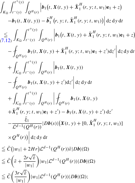 (7.18)
 -
(3)
the flow across the surface \((0,{\tilde{{\varvec{X}}}}^H_1(r,y;t,w_1)) \times [-Hr,Hr] \times \partial B^{d-2}_r(0)\): if \({\varvec{b}}^\perp \) is the component not 1 or 2, then, as above,
$$\begin{aligned} \begin{aligned}&\quad \qquad \qquad \int _{K_\Omega } \int _{t^-(y)}^{t^+(y)} \int _{(0,{\tilde{{\varvec{X}}}}^H_1(r,y;t,w_1)) \times [-Hr,Hr] \times \partial B^{d-2}_r(0)} \big | {\varvec{b}}^\perp (t,{\varvec{X}}(t,y) + z)\\&\qquad \qquad \qquad \qquad - {\varvec{b}}^\perp (t,{\varvec{X}}(t,y)) \big | \, \textrm{d}z \, \textrm{d}y \, \textrm{d}t \\&\qquad \text {near. inc.} \leqq {\bar{C}} \int _{{\mathcal {K}}_\Omega } \int _{(0,{\tilde{{\varvec{X}}}}^H_1(r,y;t,w_1)) \times [-Hr,Hr] \times \partial B^{d-2}_r(0)}\\ {}&\big | {\varvec{b}}^\perp (t,x + z) - {\varvec{b}}^\perp (t,x) \big | \, \textrm{d}z \, \textrm{d}x \, \textrm{d}t \\&\qquad {\tilde{{\varvec{X}}}}_1\text { contr.} \leqq {\bar{C}} \int _{(0,w_1) \times [-Hr,Hr] \times \partial B^{d-2}_r(0)} \bigg ( \int _\Omega |D {\varvec{b}}^\perp | \, \textrm{d}x \, \textrm{d}t \bigg ) |z| \, \textrm{d}z\\&\,\,(|z| \leqq 2 H r) \leqq {\bar{C}} (2 H r)^2 |w_1| {\mathcal {H}}^{d-3}(\partial B^{d-2}_r(0)) {\bar{\varepsilon }} |D{\varvec{b}}|(\Omega ) \\&\,\,\,\,\quad \qquad \quad \qquad = 4 {\bar{C}} H \frac{r {\mathcal {H}}^{d-3}(\partial B^{d-2}_r(0))}{{\mathcal {L}}^{d-2}(B^{d-2}_r(0))} |w_1| \big ( H r {\mathcal {L}}^{d-2}(B^{d-2}_r(0)) \big ) {\bar{\varepsilon }} |D{\varvec{b}}|(\Omega ) \\&\,\quad \qquad \quad \qquad \underset{(7.12)}{\leqq } {\bar{C}} C_d \sqrt{\bar{\varepsilon }} |w_1| {\mathcal {L}}^{d-1}(Q^H(r)) |D{\varvec{b}}|(\Omega ); \end{aligned} \end{aligned}$$(7.19) -
(4)
the flow across the surface \([0,{\tilde{{\varvec{X}}}}^H_1(r,y;t,w_1)] \times \{Hr\} \times B^{d-2}_r(0)\), whose normal is \({\textbf{e}}_2\):
$$\begin{aligned}{} & {} \quad \qquad \qquad \int _{K_\Omega } \int _{t^-(y)}^{t^+(y)} \int _{[0,{\tilde{{\varvec{X}}}}^H_1(r,y;t,w_1)] \times B^{d-2}_r(0)} \big | {\varvec{b}}_2(t,{\varvec{X}}(t,y) + Hr {\textbf{e}}_2 + z)\nonumber \\{} & {} \qquad \qquad \qquad \quad - {\varvec{b}}_2(t,{\varvec{X}}(t,y)) \big | \, \textrm{d}z \, \textrm{d}y \, \textrm{d}t\nonumber \\{} & {} \quad {\tilde{{\varvec{X}}}}_1\text { contr.} \leqq \int _{K_\Omega } \int _{t^-(y)}^{t^+(y)} \int _{[0,w_1] \times B^{d-2}_r(0)} \big | {\varvec{b}}_2(t,{\varvec{X}}(t,y) + H r {\textbf{e}}_2 + z)\nonumber \\{} & {} \quad \qquad \quad \qquad \quad - {\varvec{b}}_2(t,{\varvec{X}}(t,y) + H r {\textbf{e}}_2) \big | \, \textrm{d}z \, \textrm{d}y \, \textrm{d}t\nonumber \\{} & {} \quad \qquad \quad \qquad \quad + \int _{K_\Omega } \int _{t^-(y)}^{t^+(y)} \int _{[0,w_1] \times B^{d-2}_r(0)} \big | {\varvec{b}}_2(t,{\varvec{X}}(t,y) + H r {\textbf{e}}_2)\nonumber \\{} & {} \quad \qquad \quad \qquad \quad - {\varvec{b}}_2(t,{\varvec{X}}(t,y)) \big | \, \textrm{d}z \, \textrm{d}y \, \textrm{d}t\nonumber \\{} & {} \quad \text {near. inc.} \leqq {\bar{C}} \int _{[0,w_1] \times B^{d-2}_r(0)} \bigg ( \int _\Omega |D {\varvec{b}}_2| \, \textrm{d}x \, \textrm{d}t \bigg ) |z| \, \textrm{d}z\nonumber \\{} & {} \quad \qquad \quad \qquad \quad + {\bar{C}} Hr |w_1| {\mathcal {L}}^{d-2}(B^{d-2}_r(0)) |D_2 {\varvec{b}}_2|(\Omega )\nonumber \\{} & {} \quad \qquad \quad \qquad \leqq {\bar{C}} (|w_1| + r) |w_1| {\mathcal {L}}^{d-2}(B^{d-2}_r(0)) |D{\varvec{b}}|(\Omega )\nonumber \\{} & {} \quad \qquad \quad \qquad \quad + {\bar{C}} H r |w_1| {\mathcal {L}}^{d-2}(B^{d-2}_r(0)) {\bar{\varepsilon }} |D{\varvec{b}}|(\Omega )\nonumber \\{} & {} \quad \qquad \quad \qquad \leqq {\bar{C}} \bigg ( \frac{1}{H} + \frac{{\bar{\varepsilon }}}{2} \bigg ) |w_1| {\mathcal {L}}^{d-1}(Q^H(r)) |D{\varvec{b}}|(\Omega )\nonumber \\{} & {} \quad \qquad \quad \qquad \leqq {\bar{C}} C_d \sqrt{{\bar{\varepsilon }}} |w_1| {\mathcal {L}}^{d-1}(Q^H(r)) |D{\varvec{b}}|(\Omega ). \end{aligned}$$(7.20)The same for the surface \([0,w_1] \times \{- Hr\} \times B^{d-2}_r(0)\).

Summing up the estimates (7.17), (7.18), (7.19) and (7.20) we obtain the statement (7.16). \(\square \)
7.4.2 First selection of initial point in order to have continuity of the flow and disintegration
Consider a compact set \(K_{\Omega ,1} \subset K_\Omega \) of trajectories \({\varvec{X}}(t,y)\), where \(y \mapsto {\varvec{X}}(t,y) \in C([0,T],{\mathbb {R}}^d)\) is continuous in the \(C^0\)-topology, and such that the disintegration \(y \mapsto (D {\varvec{b}})_y\) is weakly continuous in the sense of measures and \(m \llcorner _{K_{\Omega ,1}} = {\mathcal {L}}^d \llcorner _{K_{\Omega ,1}}\), which means that the singular part of m has measure 0 on \(K_{\Omega _1}\).
Since we have
then it follows that if \({\mathcal {L}}^1(N) = 0\),
In particular we can assume that the initial and end sets \(\{t^-(y)\}_{y \in K_{\Omega ,1}},\{t^+(y)\}_{y \in K_{\Omega ,1}}\) have measure 0 with respect to \((D{\varvec{b}})_y\), and thus in \(K_{\Omega ,1}\) it holds that
We can also take a second compact set \(K_{\Omega ,2}\) made of Lebesgue points of \(K_{\Omega ,1}\) and such that the limits

are uniform with continuity modulus \(\omega _\textrm{dis}(r)\) (eventually changing \(\omega _{\textrm{dis}}\) of (7.22)). The total error can be taken
by Egorov and Lusin Theorems.
We thus have proved the following lemma:
Lemma 7.6
There exist two compact sets \(K_{\Omega ,2} \subset K_{\Omega ,1} \subset K_\Omega \) such that the following holds:
-
(1)
their difference in measure is small, that is
$$\begin{aligned} {\mathcal {H}}^d(K_\Omega {\setminus } K_{\Omega ,2}) < {\bar{\varepsilon }} {\mathcal {L}}^{d+1}(\Omega ); \end{aligned}$$(7.21) -
(2)
the maps \(K_{\Omega ,1} \ni y \mapsto {\varvec{X}}(t,y) \in C([0,T],{\mathbb {R}}^d)\) is continuous in the \(C^0\)-topology with modulus of continuity \(\omega _\textrm{dis}\);
-
(3)
for every \(y \in K_{\Omega ,1}\) it holds
$$\begin{aligned} (D{\varvec{b}})_y(\{t^\pm (y)\}) = 0 \end{aligned}$$and
$$\begin{aligned} y \mapsto (D{\varvec{b}})_y((t^-(y),t^+(y)) \quad \text {is continuous with modulus }\omega _\textrm{dis}; \end{aligned}$$(7.22) -
(4)
the compact set \(K_{\Omega ,2}\) is made of Lebesgue points of \(K_{\Omega ,1}\) such that
$$\begin{aligned}{} & {} \bigg | \frac{{\mathcal {L}}^d \big ( B^d_r(y) \cap K_{\Omega ,1} \big )}{{\mathcal {L}}^d(B^d_r(0))} - 1 \bigg | \leqq \omega _\textrm{dis}(r), \end{aligned}$$(7.23a) (7.23b)
 (7.23c)


7.4.3 Comparison of approximate flow with the disintegration
Aim of this part is to prove the following results:
Proposition 7.7
If \(r \leqq {\hat{r}}({\bar{\varepsilon }})\), it holds that
Proof
We estimate the difference of the approximate vector fields \(\tilde{\varvec{b}}^H_i(r,y;t,{\tilde{{\varvec{X}}}}^H_1(r,y;t,w_1))\) and the disintegration \((D_1{\varvec{b}}_i)_y w_1\) for a fixed \(w_1\) (\(>0\) for definiteness), with \(i=1,2\). The proof is given in several steps.
Step 1. By using (7.5)
where in the last step we use the definition of disintegration.
We estimate the integral
by
where \(K_{\Omega ,1}^{\textrm{in}}(y)\) are the trajectories in \(K_{\Omega ,1}\) which remain inside \(\cup _t {\varvec{X}}(t,y) + [0,\tilde{\varvec{X}}^H_1(r,y;t,w_1)] \times Q^H(r)\). Recall that we denote with \({\mathcal {K}}_\Omega \) the union of the graph of the trajectories starting in \(K_\Omega \), and the same with \({\mathcal {K}}_{\Omega ,1}\).
Step 2. We write the last term of (7.25) as
We have
-
(1)
term \(K^{\textrm{in}}_{\Omega ,1}(y)\): in this set the measure \((D_1{\varvec{b}}_i)_z\) are continuous by (7.22) and the trajectories remain inside the set by the definition of \(K^{\textrm{in}}_{\Omega ,1}(y)\), so that
$$\begin{aligned}{} & {} \int _{K_{\Omega ,2}} \bigg | \frac{1}{|w_1| {\mathcal {L}}^{d-1}(Q^H(r))} \int _{K_{\Omega ,1}^{\textrm{in}}(y)} [\dots ] m(\textrm{d}z)\\ {}{} & {} - (D_1 {\varvec{b}}_{1,2})_y((t^-(y),t^+(y))) \bigg | \, \textrm{d}y \\ \text {traj. are inside}{} & {} \underset{m\llcorner _{K_{\Omega ,1}} \ll {\mathcal {L}}^d}{=} \int _{K_{\Omega ,2}} \bigg | \frac{1}{|w_1| {\mathcal {L}}^{d-1}(Q^H(r))}\\ {}{} & {} \quad \int _{K_{\Omega ,1}^{\textrm{in}}(y)} (D_1 {\varvec{b}}_{1,2})_z((t^-(y),t^+(y))) \, \textrm{d}z \\{} & {} \qquad - (D_1 {\varvec{b}}_{1,2})_y((t^-(y),t^+(y))) \bigg | \, \textrm{d}y \\ (D_1{\varvec{b}}_2)_z\text { continuous}{} & {} \leqq \int _{K_{\Omega ,2}} \bigg [ \frac{{\mathcal {L}}^d(K_{\Omega ,1}^{\textrm{in}}(y))}{|w_1| {\mathcal {L}}^{d-1}(Q^H(r))} \omega _{\textrm{dis}}(Hr) \\{} & {} \quad + \bigg | (D_1 {\varvec{b}}_{1,2})_y((t^-(y),t^+(y)))\\ {}{} & {} \bigg ( \frac{{\mathcal {L}}^d(K_{\Omega ,1}^{\textrm{in}}(y))}{|w_1| {\mathcal {L}}^{d-1}(Q^H(r))} -1 \bigg ) \bigg | \bigg ] \, \textrm{d}y \\ (D_1{\varvec{b}}_2)_y\text { bounded}{} & {} \leqq \int _{K_{\Omega ,2}} \bigg [ \frac{{\mathcal {L}}^d(K_{\Omega ,1}^{\textrm{in}}(y))}{|w_1| {\mathcal {L}}^{d-1}(Q^H(r))} \omega _{\textrm{dis}}(Hr) \\{} & {} \quad + M \bigg ( 1 - \frac{{\mathcal {L}}^d(K_{\Omega ,1}^{\textrm{in}}(y))}{|w_1| {\mathcal {L}}^{d-1}(Q^H(r))} \bigg )\bigg ] \, \textrm{d}y \\ \text {see below}{} & {} \leqq \int _{K_{\Omega ,2}} \bigg [ \frac{{\mathcal {L}}^d(K_{\Omega ,1}^{\textrm{in}}(y))}{|w_1| {\mathcal {L}}^{d-1}(Q^H(r))} \omega _\textrm{dis}(Hr) \\{} & {} \quad + M \min \bigg \{ 1, \frac{\omega _\textrm{dis}(2Hr) {\mathcal {L}}^d(B^d_{2Hr}(0))}{|w_1| {\mathcal {L}}^{d-1}(Q^H(r))} \bigg \} \bigg ] \, \textrm{d}y \\{} & {} \quad + M \int _{K_{\Omega ,2}} \frac{(\text {exiting flow})}{|w_1| {\mathcal {L}}^{d-1}(Q^H(r))} \, \textrm{d}y \\ K_{\Omega ,1}^{\textrm{in}}(y) \subset S_1 \cap B^d_{2Hr}(y){} & {} \underset{(7.16)}{\leqq } 2 M \min \bigg \{ 1, \frac{\omega _\textrm{dis}(2Hr) {\mathcal {L}}^d(B^d_{2Hr}(0))}{|w_1| {\mathcal {L}}^{d-1}(Q^H(r))} \bigg \} {\mathcal {L}}^d(K_{\Omega ,2}) \\{} & {} \qquad + M {\bar{C}} \bigg ( C_d \sqrt{{\bar{\varepsilon }}} + \frac{4 r \sqrt{{\bar{\varepsilon }}}}{|w_1|} \bigg ) |D{\varvec{b}}|(\Omega ), \end{aligned}$$where we have observed that
$$\begin{aligned} \begin{aligned} z&\in [0,w_1] \times Q^H(r) {\setminus } K^{\textrm{in}}_{\Omega ,1} \\&\subset \big ( B^d_{2Hr}(0) {\setminus } K_{\Omega ,1} \big ) \cup \big ( K_{\Omega ,1} \\&\cap (\text {trajectories exiting from }\bigcup _t {\varvec{X}}(t,y) + [0,{\tilde{{\varvec{X}}}}^H_1(r,y;t,w_1)] \times Q^H(r)) \big ), \end{aligned} \end{aligned}$$and, by (7.23a),
$$\begin{aligned} {\mathcal {L}}^d \big ( B^d_{2Hr}(0) {\setminus } K_{\Omega ,1} \big ) \leqq \omega _\textrm{dis}(2Hr) {\mathcal {L}}^d(B^d_{2Hr}(0)); \end{aligned}$$ -
(2)
term \(K_\Omega {\setminus } K^{\textrm{in}}_{\Omega _1}\): these trajectories satisfy \(|(D_1 {\varvec{b}}_i)_z| \leqq M\) and exit, so that
$$\begin{aligned}{} & {} \int _{K_{\Omega ,2}} \bigg | \frac{1}{|w_1| {\mathcal {L}}^{d-1}(Q^H(r))} \int _{K_\Omega {\setminus } K^{\textrm{in}}_{\Omega _1}} [\dots ] \textrm{d}z \bigg | \, \textrm{d}y \\{} & {} \quad \leqq \frac{M}{|w_1| {\mathcal {L}}^{d-1}(Q^H(r))} \int _{K_{\Omega ,2}} \big [ m\text {-measure of exiting/entering trajectories} \big ] \, \textrm{d}y \\{} & {} \quad \leqq \frac{M}{|w_1| {\mathcal {L}}^{d-1}(Q^H(r))} \int _{K_{\Omega ,2}} \big [ \text {flow on the boundary} \big ] \, \textrm{d}y \\{} & {} \underset{(7.16)}{\leqq } \frac{M}{|w_1| {\mathcal {L}}^{d-1}(Q^H(r))} \bigg [ {\bar{C}} \bigg ( C_d \sqrt{{\bar{\varepsilon }}} + \frac{4 r \sqrt{{\bar{\varepsilon }}}}{|w_1|} \bigg ) |w_1| {\mathcal {L}}^{d-1}(Q^H(r)) |D{\varvec{b}}|(\Omega ) \bigg ] \\{} & {} \quad \leqq M {\bar{C}} \bigg ( C_d \sqrt{{\bar{\varepsilon }}} + \frac{4 r \sqrt{{\bar{\varepsilon }}}}{|w_1|} \bigg ) |D{\varvec{b}}|(\Omega ); \end{aligned}$$
Finally, collecting all estimates,
Step 3. We thus have
Step 4. Observing that
we obtain
Conclusion. For \(r< {\hat{r}} = {\hat{r}}({\bar{\varepsilon }}) < {\bar{r}}\) such that
we obtain
We have removed a set of trajectories of measure
and the estimate holds for
\(\square \)
This concludes the comparison with the disintegration, which will be used when analyzing the approximate flow with the linear one in Point (7) of page 19. Using (7.2) we have also
Corollary 7.8
It holds that
7.5 Estimates on the approximated flow
The approximated flow is defined by solving the ODE
in the time interval of interest for \({\varvec{X}}(t,y)\), that is \(t \in (t^-(y),t^+(y))\), with initial data z at \(t^-(y)\). We recall that
The first component \({\tilde{{\varvec{X}}}}^H_1(r,y;t,z)\) has already been studied in Section 7.3.
7.5.1 The part not along \({\textbf{e}}_1,{\textbf{e}}_2\)
The component of \({\tilde{{\varvec{b}}}}\) along the direction \({\textbf{e}}_{\not 1,\not 2}\) is clearly 0 because \({\bar{\xi }}\) lies in the 1, 2-plane by assumptions, so that
In particular this flow is perfectly 1-Lipschitz.
We can use Corollary A.2 to compare the real flow \({\varvec{X}}_{\not 1,\not 2}(t,y+z) - {\varvec{X}}_{\not 1,\not 2}(t,y)\) with the approximate flow until the exit time \(t^+(y;z)\) from the ball \(B^d_r(0)\).
Lemma 7.9
It holds
where \(t^+(y,z)\) is the exit time from the ball \(X(t^+(y,z),y) + B^d_r(0)\) or it coincides with the final time \(t^+(y)\).
Proof
Corollary A.2 with \({\tilde{{\varvec{b}}}} = 0\), \(L=1\) gives for all \(t \in [t^-(y),t^+(y;z)]\)
Let \(t(y,z) \in [t^-(y),t^+(y,z)]\) be such that
Integrating with respect to \(z \in B^d_r(0)\) and \(y \in K_{\Omega ,2}\) we obtain
which is (7.34). \(\square \)
Corollary 7.10
If
then
Proof
Indeed, by Chebyshev,
which is the statement. \(\square \)
Defining
where \(E_1^1(r,y)\) is defined in (7.14) and \(E^2_1(r,y)\) in (7.37), we conclude that
for \({\bar{\varepsilon }} \leqq 1\).
The estimate (7.40) gives Point (4) of page 18.
7.5.2 The part along \({\textbf{e}}_2\)
The part along \({\textbf{e}}_2\) satisfies the ODE
Since \({\tilde{{\varvec{b}}}}^H\) depends only on \(z_1\), the solution is for \(t \in [t^-(y),t^+(y,z)]\) (\(t^+(y,z)\) being the exit time from \(B^d_r(0)\))
By (7.8), we have that, for every Borel function \(z \mapsto t(y,z) \leqq t^+(y)\),
which in particular is equivalent to
Here we can allow the time t(y, z) to be larger than the exit time from the cylinder \({\varvec{X}}(t,y) + B^d_r(0)\) because of the particular form of the flow \({\tilde{{\varvec{X}}}}^H\): the first component is a contraction, and the second depends only on the first. Clearly it will be meaningless when exiting \({\varvec{X}}(t,y) + [-r,r] \times Q^H(r)\) because of the form of \({\tilde{{\varvec{b}}}}^H\).
In the following proposition, we estimate the quantity
Proposition 7.11
If \(E_1(r,y)\) is the set defined in (7.39), then it holds
This proposition corresponds to Point (5) of page 19, Equation (5.2).
Proof
In this case the flow \({\tilde{{\varvec{X}}}}_2^H\) is not Lipschitz (take for example a single jump discontinuity), so we cannot use Corollary A.2 and instead proceed as follows:
let \(t_2(y,z) \in [t^-(y),t^+(y,z)]\) be the time where
The above quantity can be written as

We have used

Integrating the third term with respect to y and using (7.2), we get
where we used the fact that \({\tilde{{\varvec{X}}}}^H_1(r,y;s,z_1) \leqq w_1 \) in the first inequality and \(|w_1| \leqq r\) in the last one.
Integrating, we obtain, for the fourth term,

The above estimate is the same for the first term:

Here in the third step we have used
valid until the exit time \(t_2(y,z)\).
Recalling that for \(z \in B^d_r(0) {\setminus } E_1(r,y)\) it holds that
we obtain (the interval in the second line may have the extremals exchanged depending on s, here for definiteness we assume \(\tilde{\varvec{X}}^H_1(r,y;s,z) \leqq {\varvec{X}}_1(s,y+z) - {\varvec{X}}_1(s,y)\))

Then integrating the second term

where we used the fact that \(B^d_r(0) {\setminus } E_1(r,y) \subset B^d_r(0)\).
Finally, collecting all estimates,
which is the statement. \(\square \)
7.6 The linearized ODE
We compare now the approximate flux \({\tilde{{\varvec{X}}}}^H(r,y;t,w)\) with the linearized flow of Section 4, namely the solution to
Let \({\tilde{W}}(t,y)\) be the solution to the following approximated ODE (whenever it exists, that is whenever \(J(t,y) \geqq c > 0\))
where \({\tilde{J}}(t,y) = \textrm{det}({\tilde{W}}(t,y))\). Clearly due to the simple form of the right-hand side one gets
Lemma 7.12
There exists a set \(K_{\Omega _3} \subset K_\Omega \) with co-measure
such that, if J(t, y) is the Jacobian of the flow \({\varvec{X}}(t,y)\) (see Proposition 3.6),
In this set the solution to (7.52) is defined for all \(t \in [t^-(y),t^+(y)]\) and it holds
Proof
We can write
Hence integrating in \(K_{\Omega }\) one obtains
Hence by Chebyshev’s inequality we can remove a set of trajectories of measure \(< \sqrt{{\bar{\varepsilon }}} |D{\varvec{b}}|(\Omega )\) and in the remaining set the estimate (7.55) holds:
In particular we deduce that
so that the solution \({\tilde{W}}(t,y)\) does exist on this set, and in the same way as in (4.14) one gets
Write for these trajectories
Integrating in time and using Duhamel Formula together with (4.4) and (7.58), we get
Integrating in \(K_{\Omega ,3}\) one deduces that
\(\square \)
The solution to (7.52) can be computed explicitly when \(y \in K_{\Omega ,3}\): the equation for the first component is
whose unique solution (from Theorem 4.1) is clearly
The only component non constant besides \({\tilde{W}}_{11}\) is \(\tilde{W}_{12}(t,y)\), which satisfies
whose solution is
Hence, we obtain
Lemma 7.13
If \(y \in K_{\Omega ,3}\), the explicit solution to (7.52) is given by
7.7 Collecting the estimates for the singular part
Here we prove that the assumptions of Section 5 are verified with the measure with a suitable measure \(\mu _P\), which will be given in Section 8, when collecting all estimates.
More precisely
-
(1)
Point (2) of page 18: there exists a set of trajectories \(S'_1 = K_{\Omega ,3}\) such that
$$\begin{aligned} \begin{aligned} {\mathcal {H}}^d(S_1 {\setminus } S'_1)&\underset{(7.21),(7.54)}{<} \bar{\varepsilon }{\mathcal {L}}^{d+1}(\Omega ) + \sqrt{\varepsilon } |D{\varvec{b}}|(\Omega )\\ {}&< ({\bar{\varepsilon }})^{1/4} \big [ |D{\varvec{b}}|(\Omega ) + {\mathcal {L}}^{d+1}(\Omega ) \big ]; \end{aligned} \end{aligned}$$(7.61) -
(2)
Point (6) of page 19: there exists an approximated solution \({\tilde{{\varvec{X}}}}^H(r,y;t,w)\) such that for all \(t \in (t^-(y),t^+(y))\), \(r' \leqq r\)
$$\begin{aligned} \begin{aligned}&\int _{K_{\Omega ,3}} \int _{B^d_{r'}(z)} \big \Vert \tilde{\varvec{X}}^H(r,y;\cdot ,w) - w \big \Vert _{C^0} \, \textrm{d}w \, \textrm{d}y\\&\quad \underset{(7.11)}{\leqq } \int _{K_\Omega } \int _{B^d_{r'}(0)} \int _{t^-(y)}^{t^+(y)} \big | {\tilde{{\varvec{b}}}}^H(r,y;s,w) \big | \, \textrm{d}s \, \textrm{d}w \, \textrm{d}y \\&\,\quad \underset{(7.8)}{\leqq } {\bar{C}} r' {\mathcal {L}}^d(B^d_{r'}(0)) |D{\varvec{b}}|(\Omega ). \end{aligned} \end{aligned}$$(7.62) -
(3)
Point (4) of page 18: for every \(y \in K_{\Omega ,3}\) there exists a set of initial points \(E_1(r,y) \subset B^d_r(0)\) such that
$$\begin{aligned} \int _{K_{\Omega ,3}} {\mathcal {L}}^d(E_1(r,y)) \, \textrm{d}y \underset{(7.40)}{<} 5 \bar{C}^2 ({\bar{\varepsilon }})^{1/4} {\mathcal {L}}^d(B^d_r(0)) |D{\varvec{b}}|(\Omega ); \end{aligned}$$(7.63) -
(4)
Formula (5.2) of Point (5), page 19: for the remaining trajectories it hold
$$\begin{aligned} \begin{aligned}&\int _{K_{\Omega ,3}} \int _{B^d_r(0) {\setminus } E_1(r,y)} \big \Vert {\varvec{X}}(\cdot ,y+z) - {\varvec{X}}(\cdot ,y)\\ {}&- {\tilde{{\varvec{X}}}}^H(r,y;\cdot ,z) \big \Vert _{C^0(t^-(y),t^+(y,z))} \, \textrm{d}z \, \textrm{d}y \\ (7.13), (7.34), (7.43)&< 3 {\bar{C}}^2 \sqrt{{\bar{\varepsilon }}} r {\mathcal {L}}^d(B^d_r(0)) |D{\varvec{b}}|(\Omega )\\&\quad + {\bar{C}}^2 r {\mathcal {L}}^d(B^d_r(0)) {\bar{\varepsilon }} |D{\varvec{b}}|(\Omega )\\ {}&+ 7 {\bar{C}} r {\mathcal {L}}^d(B^d_r(0)) ({\bar{\varepsilon }})^{1/4} |D {\varvec{b}}|(\Omega ) \\&< 11 {\bar{C}}^2 ({\bar{\varepsilon }})^{1/4} r {\mathcal {L}}^d(B^d_r(0)) |D{\varvec{b}}|(\Omega ); \end{aligned} \end{aligned}$$(7.64) -
(5)
Comparison of approximate solution with the linearised flow: recalling that
$$\begin{aligned} {\tilde{{\varvec{X}}}}^H(r,y;t,z) - z = \int _{t^-(y)}^t {\tilde{{\varvec{b}}}}^H(r,y;s,{\tilde{{\varvec{X}}}}^H_1(r,y;s,z)) \, \textrm{d}s, \end{aligned}$$(7.65)for the approximate vector field
$$\begin{aligned} \begin{aligned}&\int _{K_{\Omega ,3}} \int _{B^d_r(0)} \Big | \big ( {\tilde{{\varvec{X}}}}^H(r,y;t^+(y),w) - w \big ) - W(t^+(y),t^-(y),y) w \Big | \, \textrm{d}w \, \textrm{d}y \\&\qquad \underset{(7.60}{\leqq } \int _{K_{\Omega ,3}} \int _{B^d_r(0)} \Big | \big ( {\tilde{{\varvec{X}}}}^H(r,y;t^+(y),w) - w \big )\\ {}&\qquad \quad - {\bar{\xi }} \otimes {\bar{\eta }} |D {\varvec{b}}|_y((t^-(y),t^+(y))) w_1 \Big | \, \textrm{d}w \, \textrm{d}y \\&\qquad \qquad + \int _{B^d_r(0)} |w| \textrm{d}w \int _{K_{\Omega ,3}} \big \Vert W(\cdot ,y) - {\tilde{W}}(\cdot ,y) \big \Vert _{L^\infty (t^-(y),t^+(y))} \, \textrm{d}y \\&\underset{(7.65),(7.56)}{=} \int _{K_{\Omega ,3}} \int _{B^d_r(0)} \bigg | \int _{t^-(y)}^{t^+(y)} {\tilde{{\varvec{b}}}}^H \big ( r,y;s,{\tilde{{\varvec{X}}}}^H(r,y;s,w) \big ) \, \textrm{d}s \\&\qquad \quad \quad - {\bar{\xi }} \otimes {\bar{\eta }} |D {\varvec{b}}|_y((t^-(y),t^+(y))) w_1 \bigg | \, \textrm{d}w \, \textrm{d}y \\&\qquad \quad \quad + 3 {\bar{C}}^2 e^{3 {\bar{C}} M} \sqrt{\varepsilon } |D{\varvec{b}}|(\Omega ) \\&\,\,\underset{(7.24),(7.2)}{\leqq } C_d {\bar{C}} \sqrt{{\bar{\varepsilon }}} r {\mathcal {L}}^d(B^b_r(0)) \big [ {\mathcal {L}}^{d+1}(\Omega ) + |D{\varvec{b}}|(\Omega ) \big ]\\ {}&\qquad + {\bar{C}} r {\mathcal {L}}^d(B^d_r(0)) |D{\varvec{b}}| \big ( \Omega {\setminus } {\mathcal {K}}_0 \big ) \\&\quad \quad \qquad + 3 {\bar{C}}^2 e^{3 {\bar{C}} M} \sqrt{\varepsilon } |D{\varvec{b}}|(\Omega ). \end{aligned}\ \end{aligned}$$(7.66) -
(6)
Point (7) of page 19: if \(E_2(r,y)\) is the set of trajectories which exit from \({\varvec{X}}(t,y) + B^d_r(0)\) before \(t^+(y)\), then
$$\begin{aligned} \begin{aligned}&\int _{K_{\Omega ,2}} \int _{B^d_r(0) {\setminus } (E_1(r,y) \cup E_2(r,y))} \Big | {\varvec{X}}(t^+(y),y+z) - {\varvec{X}}(t^+(y),y) - W(t,y) z \Big | \textrm{d}z \textrm{d}y \\&\underset{(7.64), (7.66)}{<} 11 C^2 ({\bar{\varepsilon }})^{1/4} r {\mathcal {L}}^d(B^d_r(0)) |D{\varvec{b}}|(\Omega ) \\&\qquad \qquad + C_d (1 + {\bar{C}}) r {\mathcal {L}}^{d}(B^{d}_r(0)) ({\bar{\varepsilon }})^{1/4} \big [ {\mathcal {L}}^{d+1}(\Omega ) + |D{\varvec{b}}|(\Omega ) \big ] \\ {}&\qquad \qquad + {\bar{C}} r {\mathcal {L}}^d(B^d_r(0)) |D{\varvec{b}}| \big ( \Omega {\setminus } {\mathcal {K}}_0 \big ) + 3 {\bar{C}}^2 e^{3 {\bar{C}} M} \sqrt{\varepsilon } |D{\varvec{b}}|(\Omega ) \\&\qquad \quad < 16 {\bar{C}}^2 C_d r {\mathcal {L}}^{d}(B^{d}_r(0)) (\bar{\varepsilon })^{1/4} \big [ {\mathcal {L}}^{d+1}(\Omega ) + |D{\varvec{b}}|(\Omega ) \big ] \\ {}&\qquad \qquad + {\bar{C}} r {\mathcal {L}}^d(B^d_r(0)) |D{\varvec{b}}| \big ( \Omega {\setminus } {\mathcal {K}}_0 \big ). \end{aligned} \end{aligned}$$(7.67)
This concludes the local estimates in the case the singular part is contracting, that is \({\bar{\xi }} \cdot {\bar{\eta }} \leqq 0\).
7.8 The time reverse case
To study the case \({\bar{\xi }} \cdot {\bar{\eta }} > 0\), we use the estimates we have already proved by reversing time or, equivalently, by changing variables and using as initial set the set \(S_2\) instead of the set \(S_1\). In order to have more flexibility in the proof, we will choose the parameter H determining \(Q^H(r)\) later.
We proceed as follows:
-
(1)
First of all, we will consider as initial points \(S_2'\) the image of the set \(K_{\Omega ,3}\), that is \(S_2 \cap {\mathcal {K}}_{\Omega ,3}\): by the near incompressibility and the fact that up to \({\bar{C}} {\bar{\varepsilon }} {\mathcal {L}}^{d+1}(\Omega )\) all trajectories start from \(S_1\) and leave from \(S_2\) for a perturbed proper set, we obtain that
$$\begin{aligned} \begin{aligned}&{\mathcal {H}}^d(S_2 {\setminus } S'_2) \underset{(7.61),(7.1)}{<} {\bar{\varepsilon }} {\mathcal {L}}^{d+1}(\Omega ) + {\bar{C}} (\bar{\varepsilon })^{1/4} \big ( |D{\varvec{b}}|(\Omega ) + {\mathcal {L}}^{d+1}(\Omega ) \big ) \\ {}&\qquad \,\,\,\quad \qquad \qquad \underset{{\bar{\varepsilon }} \ll 1}{<} 2 {\bar{C}} (\bar{\varepsilon })^{1/4} \big ( |D{\varvec{b}}|(\Omega ) + {\mathcal {L}}^{d+1}(\Omega ) \big ). \end{aligned} \end{aligned}$$(7.68) -
(2)
We estimate the flow exiting or entering the sets
$$\begin{aligned}{} & {} \bigcup _t \big \{ {\varvec{X}}(t,y) + [0,\tilde{\varvec{X}}^H_1(r,y;t,r)] \times Q^H(r) \Big \} \quad \text {or} \nonumber \\{} & {} \bigcup _t \big \{ {\varvec{X}}(t,y) + [{\tilde{{\varvec{X}}}}^H_1(r,y;t,-r),0] \times Q^H(r) \big \}. \end{aligned}$$(7.69)One can repeat the analysis of Lemma 7.5, letting the dependence with respect to H be explicit, and obtain that the flow \(\Phi _L(y)\) is controlled by
$$\begin{aligned}{} & {} \int _{K_\Omega } \Phi _L(y) \, \textrm{d}y \underset{(7.17),(7.18),(7.19),(7.20)}{\leqq } C_d {\bar{C}} (1 + H) r {\mathcal {L}}^{d-1}(Q^H_r) {\bar{\varepsilon }} |D{\varvec{b}}|(\Omega ) \nonumber \\{} & {} \quad \leqq C_d {\bar{C}} H^2 {\bar{\varepsilon }} r^d |D{\varvec{b}}|(\Omega ). \end{aligned}$$(7.70)As usual, the constant \(C_d\) may increase line by line. Hence, if
$$\begin{aligned}{} & {} E^+(r,y) = \bigg \{ y' \in {\varvec{X}}(t^+(y),y) + B^d_r(0), y' \ \text {end point of a trajectory crossing}\\ {}{} & {} \text { the boundary of (}7.69\text {)} \bigg \}, \end{aligned}$$we have
$$\begin{aligned} \int _{K_{\Omega }} {\mathcal {L}}^d(E^+(r,y)) \, \textrm{d}y \underset{(7.70), \text { near. incompr.}}{\leqq } C_d {\bar{C}}^2 H^2 {\bar{\varepsilon }} r^d |D{\varvec{b}}|(\Omega ). \end{aligned}$$(7.71) -
(3)
By Chebyshev inequality applyed to (7.71), we remove a set of initial points \(Z_1 \subset K_{\Omega ,3}\) of measure
$$\begin{aligned} {\mathcal {H}}^d(Z_1) < {\bar{C}} \sqrt{\bar{\varepsilon }} |D{\varvec{b}}|(\Omega ), \end{aligned}$$(7.72)for the rest of the trajectories \({\varvec{X}}(t,y)\), \(y \in K_{\Omega ,3} {\setminus } Z_1\), the flow crossing the boundary of \(\bigcup _t \{{\varvec{X}}(t,y) + [0,{\tilde{{\varvec{X}}}}^H_1(r,y;t,r)] \times Q^H(r)\}\) or \(\bigcup _t \{{\varvec{X}}(t,y) + [{\tilde{{\varvec{X}}}}^H_1(r,y;t,-r),0] \times Q^H(r)\}\) is controlled by (one H in (7.70) has been incorporated in \(Q^H(r)\))
$$\begin{aligned} \Phi _L(y) \leqq C_d {\bar{C}} \sqrt{\bar{\varepsilon }} H r {\mathcal {L}}^{d-1}(Q^H_r). \end{aligned}$$(7.73)The set \(S''_2\) of final points is thus the image of \(K_{\Omega ,3} {\setminus } Z_1\), which satisfies by near incompressibility
$$\begin{aligned} \begin{aligned} {\mathcal {H}}^d(S_2 {\setminus } S''_2)&\underset{(7.68),(7.72)}{<} 2 {\bar{C}} ({\bar{\varepsilon }})^{1/4} \big [ |D{\varvec{b}}|(\Omega ) + {\mathcal {L}}^{d+1}(\Omega ) \big ] + {\bar{C}}^2 \sqrt{{\bar{\varepsilon }}} |D{\varvec{b}}|(\Omega ) \\ {}&\,\, \qquad < 3 {\bar{C}} ({\bar{\varepsilon }})^{1/4} \big [ |D{\varvec{b}}|(\Omega ) + {\mathcal {L}}^{d+1}(\Omega ) \big ]. \end{aligned} \end{aligned}$$(7.74)This is Point (2) of page 18 for the case \({\bar{\xi }} \cdot {\bar{\eta }} > 0\).
-
(4)
Using the bound (7.73), we can estimate the size of \({\tilde{{\varvec{X}}}}_1(r,y;t^+(y),r)\): by the balance
$$\begin{aligned} \text {final area} + \text {lateral flow} \geqq \frac{1}{{\bar{C}}} \text { initial trajectories}, \end{aligned}$$one gets
$$\begin{aligned} {\tilde{{\varvec{X}}}}^H_1(r,y;t^+(y),r) {\mathcal {L}}^{d-1}(Q^H(r)) + C_d {\bar{C}} H \sqrt{{\bar{\varepsilon }}} r {\mathcal {L}}^{d-1}(Q^H(r)) \geqq \frac{1}{\bar{C}} r {\mathcal {L}}^{d-1}(Q^H(r)), \end{aligned}$$where we have used (7.73). The above equation gives for \(y \in K_{\Omega ,3} {\setminus } Z_1\) that
$$\begin{aligned} {\tilde{{\varvec{X}}}}^H_1(r,y;t^+(y),r) \geqq \frac{1}{{\bar{C}}} \big ( 1 - C_d {\bar{C}}^2 \sqrt{{\bar{\varepsilon }}} H \big ) r =: r^+(r). \end{aligned}$$(7.75)This lower bound on \({\varvec{X}}^H_1(r,y;t^+(y),r)\) will be used in the next section to bound \(E^+_1(r,y)\). Note that \(r^+(r) \geqq {\mathcal {O}}(1) {\bar{C}}^{-1} r\) by the choice of H in the next points, as one has to expect from the near incompressibility (4.3).
-
(5)
We can thus estimate the subset \(E^+_1(r,y)\) of \(B^d_{r^+(r)}({\varvec{X}}(t^+(y),y))\) coming from trajectories crossing the boundary of (7.69):
$$\begin{aligned} \begin{aligned} \int _{K_{\Omega ,3} {\setminus } Z_1} {\mathcal {L}}^d(E^+_1(r,y)) \textrm{d}y&\underset{(7.71)}{\leqq } C_d {\bar{C}}^2 H^2 {\bar{\varepsilon }} r^d |D{\varvec{b}}|(\Omega ) \\&\,\,\,\,= C_d {\bar{C}}^2 H^2 {\bar{\varepsilon }} \bigg ( \frac{r}{r^+(r)} \bigg )^d {\mathcal {L}}^d(B^d_{r^+(r)}(0)) |D{\varvec{b}}|(\Omega ) \\&\underset{(7.75)}{=} \frac{C_d {\bar{C}}^{d+2} \bar{\varepsilon }H^2}{( 1 - C_d {\bar{C}}^2 \sqrt{{\bar{\varepsilon }}} H )^d} {\mathcal {L}}^d(B^d_{r^+(r)}(0)) |D{\varvec{b}}|(\Omega ). \end{aligned} \end{aligned}$$(7.76)We also estimates the set \({\varvec{X}}(t^+(y),y) + E^+_2(r,y) \subset {\varvec{X}}(t^+(y),y) + B^d_{r^+(r)}(0)\) of trajectories arriving from points which do not belongs to \({\mathcal {K}}_{\Omega ,3}\):
$$\begin{aligned} \begin{aligned} \int _{K_{\Omega ,3}} {\mathcal {L}}^d(E^+_2(r,y)) \, \textrm{d}y \underset{\text {for }r \ll 1}{\leqq } {\bar{\varepsilon }} {\mathcal {L}}^d(B^d_{r^+(r)}(0)) {\mathcal {L}}^{d+1}(\Omega ), \end{aligned} \end{aligned}$$(7.77)where we have observed that \({\mathcal {H}}^d \llcorner _{S_2}\)-almost everywhere point in \(S_2 \cap {\mathcal {K}}_{\Omega ,3}\) is a Lebesgue point. Finally we have that if
$$\begin{aligned} E^+(r,y) = E^+_1(r,y) \cup E^+_2(r,y) \end{aligned}$$then
$$\begin{aligned} \begin{aligned}&\int _{K_{\Omega ,3} {\setminus } Z_1} {\mathcal {L}}^d(E^+(r,y)) \, \textrm{d}y\\&\underset{(7.76),(7.77)}{\leqq } \frac{C_d {\bar{C}}^{d+2} {\bar{\varepsilon }} H^2}{( 1 - C_d {\bar{C}}^2 \sqrt{{\bar{\varepsilon }}} H )^d} {\mathcal {L}}^d(B^d_{r^+(r)}(0)) |D{\varvec{b}}|(\Omega ) \\ {}&\qquad \qquad \qquad + {\bar{{\varepsilon }}} {\mathcal {L}}^d(B^d_{r^+(r)}(0)) {\mathcal {L}}^{d+1}(\Omega ). \end{aligned} \end{aligned}$$ -
(6)
The remaining trajectories in \({\varvec{X}}(t^+(y),y) + B^d_{r^+(r)}(0)\) are arriving from some set which we denote as
$$\begin{aligned}{} & {} {\varvec{X}}(t^-(y),y) + A(y) \subset {\varvec{X}}(t^-(y),y) + [-r,r]\\ {}{} & {} \times Q^H(r) \subset {\mathcal {K}}_{\Omega ,3} \cap \big ( y + B^d_{(1+H)r}(0) \big ), \end{aligned}$$and are not crossing the boundary of (7.69); hence these trajectories cannot arrive from \(E_2((1+H)r,y))\), being the latter defined as the set of trajectories in \({\varvec{X}}(t^-(y),y) + B^d_{(1+H) r}(0)\) which exit \({\varvec{X}}(t,y) + B^d_r(0)\) before \(t^+(y)\). Thus by changing the coordinates from the initial points y, z at time \(t^-(y)\) to the end points at time \(t^+(y)\) and using the near incompressibility we can write
$$\begin{aligned} \begin{aligned}&\int _{K_{\Omega ,3}} \int _{A(y) {\setminus } E_1((1+H)r,y)} \Big | {\varvec{X}}(t,y+z) - {\varvec{X}}(t,y) - W(t^+(y),t^-(y),y) z \Big | \, \textrm{d}y \, \textrm{d}z \\&\underset{(4.3),(7.79)}{\geqq } \frac{1}{{\bar{C}}^2} \int _{{\varvec{X}}(K_{\Omega ,3})} \int _{B^d_{r^+(r)}(0) {\setminus } E(r^+(r),y')} \Big | w - W(t^+(y),t^-(y),y) \\&\qquad \quad \big ( {\varvec{X}}^{-1}(y'+w) - {\varvec{X}}^{-1}(y') \big ) \Big | \, \textrm{d}w \, \textrm{d}y' \\&\underset{\begin{array}{c} |(D{\varvec{b}})_y| \leqq M, \\ \text {Thm. } 4.1 \end{array}}{\geqq } \frac{e^{- {\bar{C}} M}}{\bar{C}^2} \int _{{\varvec{X}}(K_{\Omega ,3})} \int _{B^d_{r^+(r)}(0) {\setminus } E(r^+(r),y')} \Big | {\varvec{X}}^{-1}(y'+w) - {\varvec{X}}^{-1}(y')\\&\quad \qquad - W^{-1}(t^-(y),t^+(y),y) w \Big | \, \textrm{d}w \, \textrm{d}y'. \end{aligned} \end{aligned}$$(7.78)For shortness we have used the notation \(y(y')\) inverting the function
$$\begin{aligned} {\varvec{X}}\big ( t^+(y(y')),y(y') \big ) = y'. \end{aligned}$$The set \(E(r^+(r),y)\) is the set not covered by the trajectories starting in \({\varvec{X}}(t^-(y),y) + B^d_{(1+H)r}(0)\), which satisfy the estimate for which we can use (7.67): using again that the exiting trajectories have already been counted in \(E^+_1(r^+(r),y)\)
$$\begin{aligned} \begin{aligned} E(r^+(r),y)&= E_1^+(r,y) \cup E_2^+(r,y) \cup \Big [ \Big ( {\varvec{X}}\big ( t^+(y), y + E_1((1+H) r,y) \\ {}&\cup E_2((1+H)r,y) \big ) - {\varvec{X}}(t^+(y),y) \Big ) \cap B^d_{r^+(r)}(0) \Big ] \\&= E_1^+(r,y) \cup E_2^+(r,y) \\ {}&\cup \Big [ \Big ( {\varvec{X}}\big ( t^+(y), y + E_1((1+H)r,y) \big ) - {\varvec{X}}(t^+(y),y) \Big ) \cap B^d_{r^+(r)}(0) \Big ]. \end{aligned} \end{aligned}$$(7.79) -
(7)
Noting that
$$\begin{aligned} W^{-1}(t^+(y),t^-(y),y) = W(t^-(y),t^+(y),{\varvec{X}}(t^+(y),y)) = W(t^-(y'),t^+(y'),y'), \end{aligned}$$the bound (7.67) with r replaced with \((1+H) r\) gives
$$\begin{aligned} \begin{aligned}&\frac{e^{- {\bar{C}} M}}{{\bar{C}}^2} \int _{{\varvec{X}}(K_{\Omega ,3} {\setminus } Z_1)} \int _{B^d_{r^+(r)}(0) {\setminus } E(r^+(r),y')}\!\!\!\!\!\!\!\!\!\!\!\!\!\!\!\! \Big | {\varvec{X}}^{-1}(y'+w) - {\varvec{X}}^{-1}(y')\\&\qquad - W(t^-(y'),t^+(y'),y') w \Big | \, \textrm{d}w \, \textrm{d}y' \\&\underset{(7.78)}{\leqq } \int _{K_{\Omega ,3} {\setminus } Z_1} \int _{A(y) {\setminus } E_1((1+H)r,y)}\!\!\!\!\!\!\!\!\!\!\!\!\!\!\!\!\!\!\!\!\!\! \Big | {\varvec{X}}(t,y+z) - {\varvec{X}}(t,y) - W(t^+(y),t^-(y),y) z \Big | \, \textrm{d}y \, \textrm{d}z \\&\underset{A(y) \subset [-r,r] \times Q^H(r)}{\leqq } \int _{K_{\Omega ,3} {\setminus } Z_1} \int _{B^d_{(1+H)r}(0) {\setminus } (E_1((1+H)r,y) \cup E_2((1+H)r,y))} \!\!\!\!\!\!\!\!\!\!\!\!\!\!\!\!\!\!\!\!\!\!\!\!\!\!\!\!\!\!\!\!\!\!\!\!\!\!\!\!\!\!\!\!\!\!\!\!\!\!\!\!\!\!\Big | {\varvec{X}}(t,y+z) - {\varvec{X}}(t,y) \\&\qquad - W(t^+(y),t^-(y),y) z \Big | \, \textrm{d}y \, \textrm{d}z \\&\underset{(7.67)}{\leqq } 16 {\bar{C}}^2 C_d r {\mathcal {L}}^{d}(B^{d}_r(0)) ({\bar{\varepsilon }})^{1/4} \big [ {\mathcal {L}}^{d+1}(\Omega ) + |D{\varvec{b}}|(\Omega ) \big ]\\ {}&\qquad + {\bar{C}} r {\mathcal {L}}^d(B^d_r(0)) |D{\varvec{b}}| \big ( \Omega {\setminus } {\mathcal {K}}_0 \big ) \\&\quad = 16 {\bar{C}}^2 C_d (1+H)^{d+1} \bigg ( \frac{r}{r^+(r)} \bigg )^{d+1} r^+(r) {\mathcal {L}}^{d}(B^{d}_{r^+(r)}(0)) ({\bar{\varepsilon }})^{1/4}\\ {}&\quad \qquad \big [ {\mathcal {L}}^{d+1}(\Omega ) + |D{\varvec{b}}|(\Omega ) \big ] \\&\qquad + {\bar{C}} \bigg ( \frac{r}{r^+(r)} \bigg )^{d+1} r^+(r) {\mathcal {L}}^d(B^d_{r^+(r)}(0)) |D{\varvec{b}}| \big ( \Omega {\setminus } {\mathcal {K}}_0 \big ) \\&\underset{(7.75)}{=} 16 C_d \frac{({\bar{C}})^{d+3} (1+H)^{d+1}}{( 1 - C_d {\bar{C}}^2 \sqrt{{\bar{\varepsilon }}} H)^d} ({\bar{\varepsilon }})^{1/4} {\mathcal {L}}^{d}(B^{d}_{r^+(r)}(0)) \big [ {\mathcal {L}}^{d+1}(\Omega ) + |D{\varvec{b}}|(\Omega ) \big ] \\&\qquad + {\bar{C}} \bigg ( \frac{{\bar{C}}}{1 - C_d {\bar{C}}^2 \sqrt{\bar{\varepsilon }} H} \bigg )^{d+1} r^+(r) {\mathcal {L}}^d(B^d_{r^+(r)}(0)) |D{\varvec{b}}| \big ( \Omega {\setminus } {\mathcal {K}}_0 \big ). \end{aligned} \end{aligned}$$(7.80) -
(8)
Choosing
$$\begin{aligned} H = ({\bar{\varepsilon }})^{-1/16(d+1)} \gg 1, \end{aligned}$$(7.81)we obtain that
$$\begin{aligned} r^+(r) \underset{(7.75)}{=} \frac{1}{{\bar{C}}} \big ( 1 - C_d {\bar{C}}^2 ({\bar{\varepsilon }})^{(8d+7)/(16d+16)} \big ) r \end{aligned}$$and the estimate of (7.76) becomes
$$\begin{aligned} \begin{aligned}&\int _{K_{\Omega }} {\mathcal {L}}^d(E^+(r,y)) \, \textrm{d}y \\ {}&= \frac{C_d (\bar{C})^{d+2} ({\bar{\varepsilon }})^{(8d+7)/(8d+8)}}{( 1 - C_d {\bar{C}}^2 (\bar{\varepsilon })^{(8d+7)/(16d+16)})^d} {\mathcal {L}}^d(B^d_{r^+(r)}(0)) |D{\varvec{b}}|(\Omega ). \end{aligned} \end{aligned}$$(7.82)The image of the set \(E_1((1+H)r,y)\) is controlled by (7.63): hence using the nearly incompressibility its image has are controlled by
$$\begin{aligned}{} & {} \int _{K_{\Omega ,2}} {\mathcal {L}}^d({\varvec{X}}(t^+(y),t^-(y),E_1(r,y))) \, \textrm{d}y\nonumber \\ {}{} & {} \underset{(7.63)}{\leqq } 5 {\bar{C}}^3 (\bar{\varepsilon })^{1/4} {\mathcal {L}}^d(B^d_r(0)) |D{\varvec{b}}|(\Omega ), \end{aligned}$$(7.83)so that we conclude with
$$\begin{aligned} \begin{aligned}&\int _{K_{\Omega ,3}} {\mathcal {L}}^d(E(r^+,y)) \, \textrm{d}y \underset{(7.82),(7.83)}{\leqq } \frac{C_d ({\bar{C}})^{d+2} ({\bar{\varepsilon }})^{(8d+7)/(8d+8)}}{( 1 - C_d {\bar{C}}^2 ({\bar{\varepsilon }})^{(8d+7)/(16d+16)})^d}\\ {}&\qquad {\mathcal {L}}^d(B^d_{r^+(r)}(0) |D{\varvec{b}}|(\Omega ) \\&\qquad + 5 {\bar{C}}^3 ({\bar{\varepsilon }})^{1/4} {\mathcal {L}}^d(B^d_{(1+H)r}(0) |D{\varvec{b}}|(\Omega ) \\&\quad ((1+H) \leqq 2H) = \frac{C_d ({\bar{C}})^{d+2} ({\bar{\varepsilon }})^{(4d+3)/(8d+8)}}{( 1 - C_d {\bar{C}}^2 ({\bar{\varepsilon }})^{(8d+7)/(16d+16)})^d}\\ {}&\qquad {\mathcal {L}}^d(B^d_{r^+(r)}({\varvec{X}}(t^+(y),y))) |D{\varvec{b}}|(\Omega ) \\&\qquad + 5 {\bar{C}}^3 2^d ({\bar{\varepsilon }})^{(3d+4)/(16d+16)} {\mathcal {L}}^d(B^d_{r^+(r)}({\varvec{X}}(t^+(y),y))) |D{\varvec{b}}|(\Omega ). \end{aligned} \end{aligned}$$(7.84)Up to pushing the measure \({\mathcal {L}}^d(\textrm{d}y)\) to the end points \({\varvec{X}}(t^+(y),t^-(y),y))\) (thus multiplying the right-hand side by \({\bar{C}}\) when integrating in \({\mathcal {L}}^d(\textrm{d}y')\)), the estimate (7.84) corresponds to Point (3) of page 18, as well as the evaluation of the measure of \(E_2(r,y)\) of Point (7) for the expanding case. We note in particular that the fraction of \(E_2(r,y)\) can be made small around a large set of initial points: this is what is proved here for the final points, but the argument can be repeated also in the contractive case.
-
(9)
The remaining trajectories start in \(B^d_{(1+H)r}(y) {\setminus } (E_1((1+H)r,y) \cup E_2((1+H)r,y))\), because of the choice of \(E(r^+,y)\) and the assumptions that they do not leave \(B^d_{(1+H)r}(0)\). Hence we can use (7.80) together with (7.81) to obtain
$$\begin{aligned}{} & {} \int _{{\varvec{X}}(K_\Omega )} \int _{B^d_{r^+(r)} {\setminus } E(r^+,y')} \Big | {\varvec{X}}^{-1}(y'+z) - {\varvec{X}}^{-1}(y) - W(t^-(y'),t^+(y'),y) z \Big | \, \textrm{d}y' \, \textrm{d}z \nonumber \\{} & {} \underset{(7.80)}{\leqq } 16 C_d \frac{({\bar{C}})^{d+3} (1+H)^{d+1}}{( 1 - C_d {\bar{C}}^2 \sqrt{{\bar{\varepsilon }}} H)^d} ({\bar{\varepsilon }})^{1/4} {\mathcal {L}}^{d}(B^{d}_{r^+(r)}(0)) \big [ {\mathcal {L}}^{d+1}(\Omega ) + |D{\varvec{b}}|(\Omega ) \big ] \nonumber \\{} & {} + {\bar{C}} \bigg ( \frac{{\bar{C}}}{1 - C_d {\bar{C}}^2 \sqrt{{\bar{\varepsilon }}} H} \bigg )^{d+1} r^+(r) {\mathcal {L}}^d(B^d_{r^+(r)}(0)) |D{\varvec{b}}| \big ( \Omega {\setminus } {\mathcal {K}}_0 \big ) \nonumber \\{} & {} \underset{(7.81)}{=} 16 C_d \frac{2^{d+1} {\bar{C}}^{d+3} ({\bar{\varepsilon }})^{3/16}}{( 1 - C_d {\bar{C}}^2 ({\bar{\varepsilon }})^{(8d+7)/(16d+16)})^d} {\mathcal {L}}^{d}(B^{d}_{r^+(r)}(0)) \big [ {\mathcal {L}}^{d+1}(\Omega ) + |D{\varvec{b}}|(\Omega ) \big ] \nonumber \\{} & {} + {\bar{C}} \bigg ( \frac{{\bar{C}}}{1 - C_d {\bar{C}}^2 (\bar{\varepsilon })^{(8d+7)/(16d+16)}} \bigg )^{d+1} r^+(r) {\mathcal {L}}^d(B^d_{r^+(r)}(0)) |D{\varvec{b}}| \big ( \Omega {\setminus } {\mathcal {K}}_0 \big ). \end{aligned}$$(7.85)Since the trajectories not in \(E(r^+,y)\) are not exiting, we can just use Point (7) of page 19 for the previous two points: (5.3) follows from the properties of the disintegration applied to the linear flow \(W(\cdot ,y)\).
This concludes the proof that the assumptions of Section 5 hold around Lebesgue points of the singular part of the derivative.
8 Construction of a Suitable Partition into Proper Sets
The differentiability in measure follows from the estimates in the previous sections if we can find a suitable partition into perturbed proper sets such that the assumptions of Section 5 hold.
Theorem 8.1
For every open set \(\Omega \supset {\mathcal {K}}_0\) there exists a finite partition \(\{\Omega ^\textrm{sing}_i\}_{i=1}^N \cup \Omega ^\textrm{rem}\) of the compact set \({\mathcal {K}}_0 \Subset [0,T] \times {\mathbb {R}}^d\) made of disjoint perturbed proper sets, such that
and such that Points (2), (3) of Theorem 3.4 hold with \(\varepsilon \) replaced by \({\bar{\varepsilon }} \mathcal L^{d+1}(\Omega _i)\), and \(\Omega _i^\textrm{sing}\) satisfies the assumptions of Section 7.1 and \(|D^\textrm{sing}{\varvec{b}}|(\Omega ^\textrm{rem}) < {\bar{\varepsilon }}\).
Proof
Fix \(\Omega \) open neighborhood of \({\mathcal {K}}_0\), and let \(\Omega '\) be another open set such that
Without loss of generality, we can assume that \(\Omega '\) is a proper set. The construction of a disjoint covering is done as follows:
-
(1)
Consider a Lebesgue negligible set S where \(|D^\textrm{sing}{\varvec{b}}|\) is concentrated. By Besicovitch’s Theorem (see [11, Theorem 2.17]), we can cover S with countably many disjoint closed proper balls such that the estimates of Section 7.7 and Section 7.8 hold: these are collected in Point (2) of page 49 in the proof that the partition satisfies the assumptions of Section 5.
-
(2)
Hence we can consider finitely many closed proper balls \(\{B^{d+1}_{r_i}(t_i,x_i)\}_{i=1}^N\), contained in \(\Omega '\), such that
$$\begin{aligned} |D^\textrm{sing}{\varvec{b}}| \bigg ( \Omega ' {\setminus } \bigcup _{i=1}^N B^{d+1}_{r_i}(t_i,x_i) \bigg ) < {\bar{\varepsilon }}. \end{aligned}$$ -
(3)
Being these balls at positive distance from one another and from \({\mathbb {R}}^{d+1} {\setminus } \Omega \), we can perturb them into disjoint proper balls \(\{\Omega ^\textrm{sing}_i\}_{i=1}^N\), \(\Omega ^\textrm{sing}_i \subset \Omega \), such that the estimates of Point (2) of page 49 for the singular part \(D^\textrm{sing}{\varvec{b}}\) hold with \(\varepsilon \) replaced by
$$\begin{aligned} \min \left\{ {\bar{\varepsilon }} {\mathcal {L}}^{d+1}(\Omega ^\textrm{sing}_i), \ {\bar{\varepsilon }} \frac{{\mathcal {L}}^{d+1}(\Omega ' {\setminus } \cup _{i=1}^N \Omega _i^\textrm{sing})}{N} \right\} . \end{aligned}$$(8.1) -
(4)
The complement of the union of the closure of these perturbed proper balls is the set
$$\begin{aligned} \Omega ^\textrm{rem} = \Omega ' {\setminus } \bigcup _{i=1}^N \bar{\Omega }^\textrm{sing}_i. \end{aligned}$$
In order to show that the sets \(\{\Omega ^\textrm{sing}_i, \Omega ^\textrm{rem}\}\) satisfy the statement, we just need to prove that \(\Omega ^\textrm{rem}\) is a perturbed proper set: by Lemma 3.3, it is a proper set, being the difference of two proper sets whose boundaries have empty intersection. It remains to show that the flow occurs mostly on the time-flat parts of the boundary.
To this end, we need to estimate the trajectories in \({\mathcal {K}}\) which cross \(\partial \Omega ^\textrm{rem}\) outside \(\{t = 0,T\} \cup \cup _i S_i^\textrm{sing}\cup \cup _j S^\mathrm {a.c.}_j\): indeed these are the non flat parts of the boundary of \(\Omega ^\textrm{rem}\) from which a trajectory in \({\mathcal {K}}\) may enter. We observe that these trajectories are leaving one of the \(\Omega ^\textrm{sing}_i\), \(\Omega ^\mathrm {a.c.}_j\) not from some flat parts, so that their total estimate is bounded by (8.1) by \({\bar{\varepsilon }} {\mathcal {L}}^{d+1}(\Omega ^\textrm{rem})\). \(\square \)
We conclude this section by proving that the partition constructed in Theorem 8.1 satisfies the assumptions of Section 5 with a suitable measure \(\mu _P\). This will conclude the proof of Theorem 1.1.
Proposition 8.2
The partition into perturbed proper sets \(\{\Omega ^\textrm{sing}_i\}_{i=1}^N \cup \{\Omega ^\textrm{rem}\}\) satisfies the assumptions of Section 5 with
whose total mass is of order \({\bar{\varepsilon }}^{3/16}\).
Proof
We consider separately \(\Omega ^\textrm{sing}_i\) and \(\Omega ^\textrm{rem}\).
-
(1)
Estimates for \(\Omega ^\textrm{rem}\). We can use the comparison with the a.c. part \(D^\mathrm {a.c.}{\varvec{b}}\) of \(D{\varvec{b}}\) in order to obtain the estimates for every perturbed proper set \(\Omega ^\mathrm {a.c.}_j\):
-
(a)
Point (2) of page 18: by Point (2) of page 24, restrict to a set of initial data \(S'_{1,j}\) whose co-measure is small than \({\bar{\varepsilon }} {\mathcal {L}}^{d+1}(\Omega ^\textrm{rem})\);
-
(b)
Points (4), (5), (6), (7) of page 19: By (6.7), we have the following error estimate with respect to the linear flow \(W(\cdot ,y)\) solving (6.1):
$$\begin{aligned} \begin{aligned}&\int _{S'_{1,j}} \int _{B^d_{R}(0)} \big \Vert {\varvec{X}}(\cdot ,y+z) - {\varvec{X}}(\cdot ,y)- W(\cdot ,y) z \big \Vert _{C^0(t^-(y),t^+(y,z))} \, \textrm{d}z \, \textrm{d}y \\&\underset{(6.7)}{<} {\bar{C}}^2 e^M R \omega (R) {\mathcal {L}}^d(B^d_{R}(0)) |D{\varvec{b}}|(\Omega ^\textrm{rem})\\ {}&+ {\bar{C}}^2 e^M R {\mathcal {L}}^d(B^d_{R}(0)) |(D{\varvec{b}})^\textrm{sing}|(\Omega ^\textrm{rem}) \\&\,\,\,\leqq C_d {\bar{C}}^2 R {\mathcal {L}}^d(B^d_{R}(0)) \Big ( {\bar{\varepsilon }} |D{\varvec{b}}|(\Omega ^\textrm{rem}) + |D^\textrm{sing}{\varvec{b}}|(\Omega ^\textrm{rem}) \Big ) \end{aligned} \end{aligned}$$(8.3)
for \(R \ll 1\).
-
(a)
-
(2)
Estimates for \(\Omega ^\textrm{sing}_i\). By construction, the sets \(\Omega ^\textrm{sing}_i\) satisfy the assumptions of Section 7.1. Moreover, we prove that the following properties hold true.
-
(a)
Point (2) of page 18: There exists a set of trajectories \(S'_{1,i}\) such that, for \({\bar{\varepsilon }} \ll 1\),
$$\begin{aligned} \begin{aligned} {\mathcal {H}}^d(S_{1,i} {\setminus } S'_{1,i})&\underset{(7.61),(7.74)}{<} 3 ({\bar{\varepsilon }})^{1/4} \big ( |D{\varvec{b}}|(\Omega ^\textrm{sing}_i) + {\mathcal {L}}^{d+1}(\Omega ^\textrm{sing}_i) \big ); \end{aligned} \end{aligned}$$ -
(b)
Point (6) of page 19: There exists an approximated vector solution \({\tilde{{\varvec{X}}}}^H(r,y;t,w)\) such that, for all t, \(r' \leqq r\),
$$\begin{aligned} \begin{aligned}&\int _{S'_{1,i}} \int _{B^d_{r'}(z)} \big \Vert {\tilde{{\varvec{X}}}}^H(r,y;\cdot ,z) - z \big \Vert _{C^0} \, \textrm{d}w \, \textrm{d}y\\&\underset{(7.62)}{\leqq } 2 {\bar{C}} r' {\mathcal {L}}^d(B^d_{r'}(0)) |D{\varvec{b}}|(\Omega ^\textrm{sing}_i). \end{aligned} \end{aligned}$$(8.4)We have used the estimates on the norm of conditional probabilities for the disintegration, since in the time reverse case the approximate vector field is exactly the disintegration \((D{\varvec{b}})_y\) (see Point (9) of page 47).
-
(c)
Point (4) of page 18: For every \(y \in S'_{1,i}\), there exists a set of initial points \(E_1(r,y) \subset B^d_r(0)\) such that
$$\begin{aligned} \begin{aligned} \int _{S'_{1,i}} {\mathcal {L}}^d(E_1(r,y)) \, \textrm{d}y&\underset{(7.63)}{<} ({\bar{\varepsilon }})^{1/2} {\mathcal {L}}^d(B^d_r(0)) |D{\varvec{b}}|(\Omega ^\textrm{sing}_i) \\ \end{aligned} \end{aligned}$$or
$$\begin{aligned} \begin{aligned}&\int _{S'_{1,i}} {\mathcal {L}}^d(E_1(r,y)) \, \textrm{d}y \\&\underset{(7.84)}{<} \frac{C_d ({\bar{C}})^{d+2} ({\bar{\varepsilon }})^{(4d+3)/(8d+8)}}{( 1 - C_d {\bar{C}} ({\bar{\varepsilon }})^{(8d+7)/(16d+16)})^d} {\mathcal {L}}^d(B^d_{r}(y))) |D{\varvec{b}}|(\Omega ^\textrm{sing}_i) \\&\qquad + 5 {\bar{C}}^3 2^d ({\bar{\varepsilon }})^{(4d+3)/(16d+16)} {\mathcal {L}}^d(B^d_{r}(y))) |D{\varvec{b}}|(\Omega ^\textrm{sing}_i) \\&\quad \leqq C_d ({\bar{\varepsilon }})^{3/16} {\mathcal {L}}^d(B^d_{r}(y))) |D{\varvec{b}}|(\Omega ^\textrm{sing}_i). \end{aligned} \end{aligned}$$ -
(d)
Point (5) of page 19: For the remaining trajectories, we have
$$\begin{aligned} \begin{aligned}&\int _{S'_{1,i}} \int _{B^d_r(0) {\setminus } E_1(r,y)} \big \Vert {\varvec{X}}(\cdot ,y+z) - {\varvec{X}}(\cdot ,y) - {\tilde{X}}^H(r,y;\cdot ,z) \big \Vert _{C^0(t^-(y),t^+_y(z))} \, \textrm{d}z \, \textrm{d}y \\&\underset{(7.85)}{<} 11 {\bar{C}}^2 ({\bar{\varepsilon }})^{1/4} r {\mathcal {L}}^d(B^d_r(0)) |D{\varvec{b}}|(\Omega ^\textrm{sing}_i) \\&\qquad + 14 C_d M \frac{2^{d+1} {\bar{C}}^{d+3} ({\bar{\varepsilon }})^{(3d+3)/(16d+ 16)}}{( 1 - C_d {\bar{C}} ({\bar{\varepsilon }})^{(8d+7)/(16d+16)})^d} {\mathcal {L}}^{d}(B^{d}_{r^+(r)}(0)) \big [ {\mathcal {L}}^{d+1}(\Omega ^\textrm{sing}_i) \\&\qquad + |D{\varvec{b}}|(\Omega ^\textrm{sing}_i) \big ] \\&\qquad + {\bar{C}} \bigg ( \frac{{\bar{C}}}{1 - C_d {\bar{C}}^2 ({\bar{\varepsilon }})^{(8d+7)/(16d+16)}} \bigg )^{d+1} r^+(r) {\mathcal {L}}^d(B^d_{r^+(r)}(0)) |D{\varvec{b}}| \big ( \Omega ^\textrm{sing}_i {\setminus } {\mathcal {K}}_0 \big ) \\&\quad \leqq C_d ({\bar{\varepsilon }})^{1/4} {\mathcal {L}}^d(B^d_{r}(y)) \big [ {\mathcal {L}}^{d+1}(\Omega ^\textrm{sing}_i) + |D{\varvec{b}}|(\Omega ^\textrm{sing}_i) \big ] \\&\qquad + C_d {\mathcal {L}}^d(B^d_{r}(y)) |D{\varvec{b}}|(\Omega ^\textrm{sing}_i {\setminus } {\mathcal {K}}_0). \end{aligned} \end{aligned}$$(8.5) -
(e)
Point (7) of page 19: By the choice of the singular point,
$$\begin{aligned} \begin{aligned}&\int _{S'_{1,i}} \int _{B^d_r(0) {\setminus } (E_1(r,y) \cup E_2(r,y))} \Big | {\varvec{X}}(t^+(y),y+z) - {\varvec{X}}(t^+(y),y) \\&\quad \,\,\qquad - W((t^-(y),t^+(y)),y) z \Big | \, \textrm{d}z \, \textrm{d}y \\&\underset{(7.67),(7.85)}{<} 14 C_d {\bar{C}}^2 r {\mathcal {L}}^{d}(B^{d}_r(0)) ({\bar{\varepsilon }})^{1/4} \big [ {\mathcal {L}}^{d+1}(\Omega ^\textrm{sing}_i) + |D{\varvec{b}}|(\Omega ^\textrm{sing}_i) \big ] \\&\qquad \qquad + 14 C_d M \frac{2^{d+1} {\bar{C}}^{d+3} ({\bar{\varepsilon }})^{(3d+3)/(16d+ 16)}}{( 1 - C_d {\bar{C}} ({\bar{\varepsilon }})^{(8d+7)/(16d+16)})^d} {\mathcal {L}}^{d}(B^{d}_{r^+(r)}(0)) \big [ {\mathcal {L}}^{d+1}(\Omega ^\textrm{sing}_i) \\&\qquad \qquad + |D{\varvec{b}}|(\Omega ^\textrm{sing}_i) \big ] \\&\qquad \qquad + {\bar{C}} \bigg ( \frac{{\bar{C}}}{1 - C_d {\bar{C}}^2 ({\bar{\varepsilon }})^{(8d+7)/(16d+16)}} \bigg )^{d+1} r^+(r) {\mathcal {L}}^d(B^d_{r^+(r)}(0)) |D{\varvec{b}}| \big ( \Omega ^\textrm{sing}_i {\setminus } {\mathcal {K}}_0 \big ) \\&\quad \qquad \leqq C_d ({\bar{\varepsilon }})^{1/4} {\mathcal {L}}^d(B^d_{r}(y)) \big [ {\mathcal {L}}^{d+1}(\Omega ^\textrm{sing}_i) + |D{\varvec{b}}|(\Omega ^\textrm{sing}_i) \big ] \\&\qquad \qquad + C_d {\mathcal {L}}^d(B^d_{r}(y)) |D{\varvec{b}}|(\Omega ^\textrm{sing}_i {\setminus } {\mathcal {K}}_0). \end{aligned} \end{aligned}$$
-
(a)
We then define the measure \(\mu _P\) as
whose total mass is less than \({\mathcal {O}}({\bar{\varepsilon }}^{3/16})\). This gives the Point (1) of page 18. \(\square \)
Change history
26 January 2023
Missing Open Access funding information has been added in the Funding Note.
References
Alberti, G.: Rank one property for derivatives of functions with bounded variation. Proc. R. Soc. Edinburgh Sect. A 123(2), 239–274, 1993
Alberti, G., Bianchini, S., Crippa, G.: Two-dimensional transport equation with Hamiltonian vector fields. Hyperbolic Problems: Theory, Numerics and Applications, Volume 67 of Proceedings of Symposia in Applied Mathematics. American Mathematical Society, Providence, 337–346, 2009
Alberti, G., Bianchini, S., Crippa, G.: Structure of level sets and Sard-type properties of Lipschitz maps. Ann. Sc. Norm. Super. Pisa Cl. Sci. (5) 12(4), 863–902, 2013
Alberti, G., Bianchini, S., Crippa, G.: A uniqueness result for the continuity equation in two dimensions. J. Eur. Math. Soc. (JEMS) 16(2), 201–234, 2014
Alberti, G., Crippa, G., Mazzucato, A.L.: Exponential self-similar mixing and loss of regularity for continuity equations. C. R. Math. Acad. Sci. Paris 352(11), 901–906, 2014
Alberti, G., Crippa, G., Mazzucato, A.L.: Exponential self-similar mixing by incompressible flows. J. Am. Math. Soc. 32(2), 445–490, 2019
Alberti, G., Crippa, G., Mazzucato, A.L.: Loss of regularity for the continuity equation with non-Lipschitz velocity field. Ann. PDE 5(1), 5–9, 2019
Ambrosio, L.: Transport equation and Cauchy problem for BV vector fields. Invent. Math. 158(2), 227–260, 2004
Ambrosio, L., Crippa, G.: Existence, uniqueness, stability and differentiability properties of the flow associated to weakly differentiable vector fields. Transport Equations and Multi-D Hyperbolic Conservation Laws, Volume 5 of Lecture Notes of the Unione Matematica Italiana. Springer, Berlin, 3–57, 2008
Ambrosio, L., Crippa, G.: Continuity equations and ODE flows with non-smooth velocity. Proc. R. Soc. Edinburgh Sect. A 144(6), 1191–1244, 2014
Ambrosio, L., Fusco, N., Pallara, D.: Functions of Bounded Variation and Free Discontinuity Problems. Oxford Mathematical Monographs. The Clarendon Press, Oxford University Press, New York, 2000
Ambrosio, L., Lecumberry, M., Maniglia, S.: Lipschitz regularity and approximate differentiability of the DiPerna–Lions flow. Rend. Sem. Mat. Univ. Padova 114(29–50), 2005, 2006
Ambrosio, L., Malý, J.: Very weak notions of differentiability. Proc. R. Soc. Edinburgh Sect. A 137(3), 447–455, 2007
Atkinson, K.E.: An Introduction to Numerical Analysis, 2nd edn. Wiley, New York, 1989
Bianchini, S.: On Bressan’s conjecture on mixing properties of vector fields. Self-similar Solutions of Nonlinear PDE, Volume 74 of Banach Center Publications. Institute of Mathematics of the Polish Academy of Sciences, Warsaw, 13–31, 2006
Bianchini, S., Bonicatto, P.: A uniqueness result for the decomposition of vector fields in \({\mathbb{R} }^d\). Invent. Math. 220(1), 255–393, 2020
Bianchini, S., Bonicatto, P.: Forward untangling and applications to the uniqueness problem for the continuity equation. Discrete Contin. Dyn. Syst. 41(6), 2739–2776, 2021
Bianchini, S., Bonicatto, P., Gusev, N.A.: Renormalization for autonomous nearly incompressible BV vector fields in two dimensions. SIAM J. Math. Anal. 48(1), 1–33, 2016
Bianchini, S., Gloyer, M.: An estimate on the flow generated by monotone operators. Commun. Partial Differ. Equ. 36(5), 777–796, 2011
Bianchini, S., Gusev, N.A.: Steady nearly incompressible vector fields in two-dimension: chain rule and renormalization. Arch. Ration. Mech. Anal. 222(2), 451–505, 2016
Bohun, A., Bouchut, F., Crippa, G.: Lagrangian flows for vector fields with anisotropic regularity. Ann. Inst. H. Poincaré Anal. Non Linéaire 33(6), 1409–1429, 2016
Bonicatto, P., Gusev, N.A.: On the structure of divergence-free measures on \({\mathbb{R}}^2\). arXiv:1912.10936, 2019
Bonicatto, P., Marconi, E.: Regularity estimates for the flow of BV autonomous divergence-free vector fields in \({\mathbb{R} }^2\). Commun. Partial Differ. Equ. 46(12), 2235–2267, 2021
Bouchut, F., Crippa, G.: Lagrangian flows for vector fields with gradient given by a singular integral. J. Hyperbolic Differ. Equ. 10(2), 235–282, 2013
Bressan, A.: The unique limit of the Glimm scheme. Arch. Ration. Mech. Anal. 130(3), 205–230, 1995
Bressan, A.: Hyperbolic systems of conservation laws. The One-Dimensional Cauchy Problem, Volume 20 of Oxford Lecture Series in Mathematics and Its Applications (Ed. Bressan A.) Oxford University Press, Oxford, 2000
Bressan, A.: An ill posed Cauchy problem for a hyperbolic system in two space dimensions. Rend. Sem. Mat. Univ. Padova 110, 103–117, 2003
Bressan, A.: A lemma and a conjecture on the cost of rearrangements. Rend. Sem. Mat. Univ. Padova 110, 97–102, 2003
Brué, E., Nguyen, Q.-H.: Advection diffusion equations with Sobolev velocity field. Commun. Math. Phys. 383(1), 465–487, 2021
Bruè, E., Nguyen, Q.-H.: Sharp regularity estimates for solutions of the continuity equation drifted by Sobolev vector fields. Anal. PDE 14(8), 2539–2559, 2021
Bruè, E., Nguyen, Q.-H., Stefani, G.: A maximal function characterisation of absolutely continuous measures and Sobolev functions. Atti Accad. Naz. Lincei Rend. Lincei Mat. Appl. 30(3), 599–614, 2019
Colombini, F., Lerner, N.: Uniqueness of continuous solutions for BV vector fields. Duke Math. J. 111(2), 357–384, 2002
Crippa, G., De Lellis, C.: Estimates and regularity results for the DiPerna–Lions flow. J. Reine Angew. Math. 616, 15–46, 2008
Crippa, G., Ligabue, S.: A note on the Lagrangian flow associated to a partially regular vector field. Differ. Equ. Dyn. Syst. 1–20, 2020
Crippa, G., Lucà, R., Schulze, C.: Polynomial mixing under a certain stationary Euler flow. Physica D 394, 44–55, 2019
Crippa, G., Schulze, C.: Cellular mixing with bounded palenstrophy. Math. Models Methods Appl. Sci. 27(12), 2297–2320, 2017
De Lellis, C.: Notes on hyperbolic systems of conservation laws and transport equations. Handbook of Differential Equations: Evolutionary Equations, Handbook of Differential Equations, Vol. III. Elsevier/North-Holland, Amsterdam, 277–382, 2007
De Lellis, C.: A note on Alberti’s rank-one theorem. Transport Equations and Multi-D Hyperbolic Conservation Laws, Volume 5 of Lecture Notes Unione Matematica Italiana. Springer, Berlin, 61–74, 2008
De Philippis, G., Rindler, F.: On the structure of \({\cal{A} }\)-free measures and applications. Ann. Math. (2) 184(3), 1017–1039, 2016
DiPerna, R.J., Lions, P.-L.: Ordinary differential equations, transport theory and Sobolev spaces. Invent. Math. 98(3), 511–547, 1989
Elgindi, T.M., Zlatoš, A.: Universal mixers in all dimensions. Adv. Math. 356, 106807, 2019
Fremlin, D.H.: Measure Theory. Volume 4. Topological Measure Spaces. Part I, II. Torres Fremlin, Colchester, 2006. Corrected second printing of the 2003 original
Hadžić, M., Seeger, A., Smart, C.K., Street, B.: Singular integrals and a problem on mixing flows. Ann. Inst. H. Poincaré Anal. Non Linéaire 35(4), 921–943, 2018
Iyer, G., Kiselev, A., Xu, X.: Lower bounds on the mix norm of passive scalars advected by incompressible enstrophy-constrained flows. Nonlinearity 27(5), 973–985, 2014
Jabin, P.-E.: Differential equations with singular fields. J. Math. Pures Appl. (9) 94(6), 597–621, 2010
Le Bris, C., Lions, P.-L.: Renormalized solutions of some transport equations with partially \(W^{1,1}\) velocities and applications. Ann. Mat. Pura Appl. (4) 183(1), 97–130, 2004
Léger, F.: A new approach to bounds on mixing. Math. Models Methods Appl. Sci. 28(5), 829–849, 2018
Lerner, N.: Transport equations with partially \(BV\) velocities. Ann. Sc. Norm. Super. Pisa Cl. Sci. (5) 3(4), 681–703, 2004
Lin, Z., Thiffeault, J.-L., Doering, C.R.: Optimal stirring strategies for passive scalar mixing. J. Fluid Mech. 675, 465–476, 2011
Lunasin, E., Lin, Z., Novikov, A., Mazzucato, A., Doering, C.R.: Optimal mixing and optimal stirring for fixed energy, fixed power, or fixed palenstrophy flows. J. Math. Phys. 53(11), 115611, 2012
Lunasin, E., Lin, Z., Novikov, A., Mazzucato, A., Doering, C.R.: Erratum: “Optimal mixing and optimal stirring for fixed energy, fixed power, or fixed palenstrophy flows’’ [J. Math. Phys. 53, 115611 (2012)] [MR3026556]. J. Math. Phys. 54(7), 079903, 3, 2013
Massaccesi, A., Vittone, D.: An elementary proof of the rank-one theorem for BV functions. J. Eur. Math. Soc. (JEMS) 21(10), 3255–3258, 2019
Nguyen, Q.-H.: Quantitative estimates for regular Lagrangian flows with \(BV\) vector fields. Commun. Pure Appl. Math. 74(6), 1129–1192, 2021
Schlichting, A., Seis, C.: Convergence rates for upwind schemes with rough coefficients. SIAM J. Numer. Anal. 55(2), 812–840, 2017
Schlichting, A., Seis, C.: Analysis of the implicit upwind finite volume scheme with rough coefficients. Numer. Math. 139(1), 155–186, 2018
Seis, C.: Maximal mixing by incompressible fluid flows. Nonlinearity 26(12), 3279–3289, 2013
Seis, C.: A quantitative theory for the continuity equation. Ann. Inst. H. Poincaré Anal. Non Linéaire 34(7), 1837–1850, 2017
Seis, C.: Optimal stability estimates for continuity equations. Proc. R. Soc. Edinburgh Sect. A 148(6), 1279–1296, 2018
Seis, C.: Diffusion limited mixing rates in passive scalar advection. arXiv:2003.08794, 2020
Smirnov, S.K.: Decomposition of solenoidal vector charges into elementary solenoids, and the structure of normal one-dimensional flows. Algebra i Analiz 5(4), 206–238, 1993
Stepanov, E., Trevisan, D.: Three superposition principles: currents, continuity equations and curves of measures. J. Funct. Anal. 272(3), 1044–1103, 2017
Yao, Y., Zlatoš, A.: Mixing and un-mixing by incompressible flows. J. Eur. Math. Soc. (JEMS) 19(7), 1911–1948, 2017
Acknowledgements
The authors are members of the Gruppo Nazionale per l’Analisi Matematica, la Probabilità e le loro Applicazioni (GNAMPA) of the Istituto Nazionale di Alta Matematica (INdAM). N. De Nitti is partially supported by the Alexander von Humboldt Fundation and by TRR-154 Project of the Deutsche Forschungsgemeinschaft (German Research Foundation, DFG); he acknowledges the kind hospitality and financial support received from SISSA within the framework of the Research Training Fellowship for Undergraduate Students 2018, during which part of this work was carried out. We would also like to thank Paolo Bonicatto and Giuseppe Maria Coclite for several conversations on topics related to this work and the anonymous referees for their helpful comments that contributed to improve the quality of the manuscript.
Funding
Open Access funding enabled and organized by Projekt DEAL.
Author information
Authors and Affiliations
Corresponding authors
Additional information
Communicated by C. Le Bris.
Publisher's Note
Springer Nature remains neutral with regard to jurisdictional claims in published maps and institutional affiliations.
Appendix A. Bressan’s Lemma on the Approximation of Lipschitz Continuous Flows
Appendix A. Bressan’s Lemma on the Approximation of Lipschitz Continuous Flows
A key tool in the proof of our main result is the following lemma (see [25, Lemma 4] or [26, Theorem 2.9]): given an absolutely continuous curve \(\gamma \) and a Lipschitz continuous semigroup \(S_t\), we can estimate the distance between \(\gamma \) and the trajectory of the semigroup starting at \(\gamma (0)\).
Lemma A.1
Let \(t \mapsto \gamma (t)\) be an a.c. curve, and \(S_t\) is a L-Lipschitz semigroup. If there exists an \(L^1\)-function \(f : {\mathbb {R}}^+ \rightarrow {\mathbb {R}}^+\) such that
then
Proof
Let us consider the curve
We have
Using the assumption on \(S_t\), we have
so that the curve is absolutely continuous. Moreover, in each point of differentiability,
which concludes the proof. \(\square \)
We use Lemma A.1 to compare a nearly incompressible flow \({\varvec{X}}(t,y)\) generated by a vector field \({\varvec{b}}\) with a L-Lipschitz flow \({\varvec{Y}}(t,y)\) generated by the vector field \(\varvec{{\tilde{b}}}\) that satisfies
on a set of full \({\mathcal {L}}^{d+1}\)-measure.
Corollary A.2
If \({\varvec{X}}(t,y)\) is a nearly incompressible flow generated by \({\varvec{b}}(t,x)\) and \({\varvec{Y}}(t,y)\) is a L-Lipschitz continuous semigroup such that (A.1) holds for \({\mathcal {L}}^{d+1}\)-almost everywhere \((t,x) \in [0,T]\times {\mathbb {R}}^d\), then, for \({\mathcal {L}}^d\)-almost everywhere \(y \in {\mathbb {R}}^d\),
Proof
Lemma A.1 yields
By the nearly incompressibility and Fubini theorem, for \({\mathcal {L}}^d\)-almost everywhere trajectory the above limit is equal for \({\mathcal {L}}^1\)-almost everywhere t to \(|{\varvec{b}}(t,{\varvec{X}}(t,y)) - {\tilde{{\varvec{b}}}}(t,{\varvec{X}}(t,y))|\). We thus proved the claim. \(\square \)
In particular, we remark that assumption (A.1) holds in the following two cases (which are relevant to Sections 6 and 7 respectively):
-
(1)
the linear flow generated by a matrix \(A(t) \in L^1((0,T))\);
-
(2)
the solution to the differential inclusion
$$\begin{aligned} \dot{x} \in - A(t,x), \end{aligned}$$with A(t) a quasi monotone operator defined in \({\mathbb {R}}^d\) and such that \(|A(t,0)| \in L^1\).
The first case is elementary; the second one is analyzed in [19].
Rights and permissions
Open Access This article is licensed under a Creative Commons Attribution 4.0 International License, which permits use, sharing, adaptation, distribution and reproduction in any medium or format, as long as you give appropriate credit to the original author(s) and the source, provide a link to the Creative Commons licence, and indicate if changes were made. The images or other third party material in this article are included in the article’s Creative Commons licence, unless indicated otherwise in a credit line to the material. If material is not included in the article’s Creative Commons licence and your intended use is not permitted by statutory regulation or exceeds the permitted use, you will need to obtain permission directly from the copyright holder. To view a copy of this licence, visit http://creativecommons.org/licenses/by/4.0/.
About this article

Cite this article
Bianchini, S., De Nitti, N. Differentiability in Measure of the Flow Associated with a Nearly Incompressible BV Vector Field. Arch Rational Mech Anal 246, 659–734 (2022). https://doi.org/10.1007/s00205-022-01820-1
Received:
Accepted:
Published:
Issue Date:
DOI: https://doi.org/10.1007/s00205-022-01820-1