
Abstract
With the continuous development of smart grid construction and the gradual improvement of power market operation mechanisms, the importance of power load forecasting is continually increasing. In this study, a short-term load prediction method based on the fuzzy optimization combined model of load feature recognition was designed to address the problems of weak generalization ability and poor prediction accuracy of the conventional feedforward neural network prediction model. First, the Douglas–Peucker algorithm and fuzzy optimization theory of load feature recognition were analyzed, and the combined prediction model was constructed. Second, data analysis and pre-processing were performed based on the actual historical load data of a certain area and the corresponding meteorological and calendar rule information data. Finally, a practical example was used to test and analyze the short-term load forecasting effect of the fuzzy optimization combined model. The calculation results proved that the presented fuzzy optimization combined model of load feature recognition outperformed the conventional model in terms of computational efficiency and specific performance; therefore, the proposed model supports further development of actual power load prediction.
1 Introduction
The short-term forecasting of power load is essential in the stable economic operation of power systems [1]. As the intelligence degree of power grids continuously increases and the power marketing mechanism gradually improves, the frequency of information interaction between the user and power grid sides increases at a wider range [2, 3]. At the grid operation level, major adjustment characteristics of the load side must be acquired at the highest possible accuracy level to guarantee the reliable operation of the system through corresponding dispatching measures. Moreover, the market operation system is more concerned with the electricity consumption characteristics of users to reasonably adjust the generation schedule and enhance competitiveness in the electricity market environment [4, 5]. Therefore, a power system under the new development background has more detailed requirements for short-term load forecasting, that is, it must not only fulfill the demand of grid production and scheduling but also describe the load characteristics with high accuracy.
With the popularization of artificial intelligence concepts and the advancement of technology, machine learning and deep learning have been widely supported and applied in short-term load forecasting research. Among them, machine learning methods such as neural networks and support vector machine regression have shown rapid development trends due to their powerful data mining capabilities and superiority in solving complex nonlinear problems [6,7,8,9]. Through the utilization of big data and advanced algorithms, these methods can discover hidden patterns and trends from historical load data, enabling accurate load forecasting. Furthermore, with the continuous progress of technology and the widespread application, the application of load forecasting methods in the power market has shown an increasingly widespread trend.
In the actual application of typical machine learning methods, such as neural networks and SVM regression, for short-term load forecasting, some problems might be encountered. First, the collected load information data are more intensive in time scale owing to the continuous refining of the level of load information collection device; simultaneously, data sources affecting short-term load forecasting, including meteorological, daily type, and economic and social factors, are gradually increasing. Therefore, the input vector for training the machine learning model of short-term load forecasting is usually extremely large, which reduces the computational efficiency. Second, when the machine learning model trained on the historical load information data is forecasting the output of a short-term load prediction curve, large prediction errors at the characteristic points of the predicted load curve might appear; therefore, prediction errors of the peak and trough of the load curve in a period are large [10]. In this study, the load characteristics primarily refer to the optimal load data subset in the original load data set that can reflect the trend law of the original load curve. Load characteristics reflect the key change trend of the load curve in a certain time interval. Indeed, we can gain insight into the internal characteristics of actual load by acquiring load characteristics. Because the load data points near the load characteristics will fluctuate and interfere within a certain numerical range of the load characteristics, the forecasting accuracy of the short-term load forecasting curve characteristics will inevitably be negatively affected. This not only restricts the further improvement of the overall accuracy of short-term load forecasting but also leads to the loss of key information on the short-term load forecasting curve. This is not conducive to the stable economic operation of the power grid and the long-term development of the power market.
In typical engineering applications of machine learning, feature selection methods can be roughly classified into filtering, wrapping, and embedding methods. Feature dimension reduction methods include the principal component and linear discriminant analyses [6, 11,12,13,14]. Although the machine learning feature engineering method has its general advantages in application, the interpretability of the finally formed load features is not clear and sufficiently intuitive. The Douglas–Peucker (DP) algorithm, as a classical method in the research of basic curve feature extraction and compression, has the advantages of high computational efficiency and strong visibility; thus, it is appropriate for the extraction and dimension reduction of load curve features. However, the threshold setting of the algorithm has some limitations on the rationality of feature extraction [15]. Therefore, this study proposes a short-term load forecasting method based on the fuzzy optimization load feature identification (recognition) combined model.
First, the load curves were analyzed using the fuzzy clustering analysis. The DP algorithm of fuzzy optimization with adaptive threshold adjustment was established to identify and extract the load characteristics of similar load curves with comparable load characteristics.
Second, the fuzzy optimization load feature recognition and machine learning models were combined to construct a combined prediction model, and the idea of classification prediction was integrated to predict the characteristics of future loads; thus, the typical predicted load curve was reconstructed.
Finally, the effectiveness of the proposed method was evaluated and discussed using an actual power system example; the obtained results verified that the proposed fuzzy optimization load feature identification combined model exhibited higher prediction performance and wider application prospects compared to those of the conventional neural network prediction model.
2 Fuzzy optimization load feature identification method
The machine learning method used in short-term load forecasting is supervised learning, and the process of training needs a considerable number of historical data samples. In addition, the core requirement of load feature extraction is to complete the accurate identification, extraction, and dimension reduction of load features on the premise of preserving the shape features of the original load curve. Figure 1 shows a schematic of the relationship between the load curve and corresponding load characteristics.

Actual load curve and load characteristics
An appropriate clustering algorithm should be employed for classification to analyze the historical load curve data samples; therefore, an optimized load feature recognition method is used to construct an accurate adaptive load feature recognition model for each class under the premise of similar characteristics for all types of in-class load curves. The process of fuzzy optimization load feature identification is shown in Fig. 2.

Schematic of fuzzy optimization load feature recognition
2.1 Fuzzy cluster analysis method
The process of the fuzzy C-means (FCM) [16] clustering analysis is described as follows:
Step 1: Initialize. Set the total set of data samples as \(X = \{ x_{j} \left| {j = 1,2, \cdots N} \right.\}\). The number of clusters is \(M(2 \le M \le N)\). Thus, \(X\) is divided into \(M(2 \le M \le N)\) classes, denoted as \(X^{1} ,X^{2} , \cdots ,X^{M}\). Therefore, \(X^{i} = \emptyset (i = 1,2, \cdots ,M),k = 1\). Meanwhile, \(M\) initial cluster centers are set, denoted as \(C = (c_{1} (k),c_{2} (k), \cdots ,c_{M} (k))\).
Step 2: Calculate the Euclidean distance \(c_{i}\) from sample A to the cluster center \(x_{j}\) using Eq. (1).
where \(t\) is the total number of clustering indicators of data samples.
Step 3: Calculate the membership \(u_{ji}\) of sample \(x_{j}\) for class \(i\) as follows:
According to the principle of minimum distance, \(X\) is clustered. Suppose that Eq. (3) is satisfied.
Moreover,\(X^{{i_{0} }} = X^{{i_{0} }} \cup \{ x_{j} \}\) for \({\kern 1pt} {\kern 1pt} i_{0} = 1,2, \ldots ,M\).
Step 4: Update the cluster center using Eq. (4).
Step 5: Assume that \(i = \{ 1,2, \cdots ,M\}\), satisfying \(c_{i} (k + 1) \ne c_{i} (k)\); subsequently, go to Step 2 and execute the process again; otherwise, the FCM clustering ends.
2.2 Douglas–Peucker algorithm
The load curves obtained using the FCM clustering exhibit large differences between classes and small differences within classes. Therefore, an appropriate curve feature recognition method is needed to identify and extract all similar load curves in a certain class one by one.
The flowchart of the classical DP algorithm [15] can be summarized as follows:
Step 1 Connect the first and last two points of the target curve with a straight line and find the vertical distance between the other points on the current target curve and the straight line.
Step 2 Set the threshold value for the DP algorithm and select the maximum vertical distance calculated in Step 1 to compare with the threshold value. If the value is greater than the threshold, the data points corresponding to the maximum vertical distance of the line are retained. Otherwise, all data points between the two ends of the line are discarded.
Step 3 Based on the retained data points, the target curve is divided into two parts for processing, and each part is treated as a new target curve. Steps 1 and 2 are repeated, and the iteration is repeated based on the idea of dichotomy, that is, the maximum vertical distance is still selected to compare with the threshold value, and the selection is successively determined until no point can be abandoned. Finally, the feature points of the curve that fulfill the predetermined accuracy threshold requirement are obtained, and other points are dropped to complete the feature extraction of the target curve.
2.3 A two-stage fuzzy optimization method for load feature recognition and extraction
This study adopts a two-stage fuzzy improved DP (TFIDP) algorithm. First, the improved DP algorithm based on the fuzzy optimization threshold is used for the initial feature extraction of load. Subsequently, the secondary feature extraction is carried out based on the primary feature extraction following the idea of statistical frequency distribution. Finally, the feature recognition and extraction of the load is completed.
2.3.1 Initial feature extraction based on the fuzzy optimization DP algorithm
In practical applications, the value of the threshold must be considered by complicated factors that are difficult to quantify. Moreover, the threshold adaptivity for different original data sets must be adjusted. Therefore, it is of great practical significance to construct a fuzzy optimal DP model with an adaptive threshold adjustment.
Based on practical experiences, the threshold in the classical DP algorithm is usually regarded as a certain value in the range of [0,1]. However, for a series of actual curves with similar shape features, a reasonable threshold should exist such that the curve features extracted from this cluster of similar curves can fulfill practical requirements. Therefore, the threshold setting of the DP algorithm is fuzzy, which is in line with the basic idea of fuzzy mathematics to describe and model fuzzy concepts through accurate mathematical means and solve practical problems properly. In summary, the classical DP algorithm is improved to introduce the concept of fuzzy mathematics in the formation of the DP algorithm of fuzzy optimization threshold \(\varepsilon\). The threshold \(\varepsilon\) in the DP algorithm is the key control factor for the final feature set extraction of curves. The introduction of a reasonable fuzzy mathematical concept to fuzzy optimization of the threshold \(\varepsilon\) can make the curve feature recognition and extraction process of the DP algorithm more universal and generalized.
The universe \(E \in [0,1]\) is defined as the threshold value region of the DP algorithm feature extraction. This study sets the threshold value in the interval [0,1], and the value interval is 0.1 to simplify the operation. Moreover, \(Sat\left( \varepsilon \right)\) represents the membership of the threshold value of the DP algorithm to a cluster of similar curves.
where the threshold membership \(Sat\left( \varepsilon \right)\) is composed of two parts, which can be seen as the overall curve feature extraction satisfaction of the specified similar curve cluster under a certain threshold; \(D\left( \varepsilon \right)\) is the average matching degree between the curve features extracted from the specified similar curve cluster and original curve, to verify whether the extracted curve features can completely reflect the shape features of the original curve; \(Z\left( \varepsilon \right)\) is the percentage ratio of the number of curve feature points to the number of original curve points, that is, the average percentage of the original curve compressed by curve feature extraction; and a and b are the corresponding proportional coefficients.
2.3.1.1 Average dynamic time warping (DTW) matching degree \(D\left( \varepsilon \right)\)
Because the time dimension of curve features is reduced compared with the original curve, and thus, it is no longer a one-to-one mapping relationship, this study introduces the DTW algorithm to calculate the matching degree between the original curve and curve features. If the original and feature sequences of the curve are \(X\) and \(Y\), the sequence lengths are \(L_{X}\) and \(L_{Y}\), respectively. The regular path is defined as \(w = [w_{1} ,w_{2} , \cdots ,w_{K} ]\), where \(w_{i} = (p_{i} ,q_{i} ) \in [1:L_{X} ] \times [1:L_{Y} ]\), \(1 \le i \le K\). The regular path needs to fulfill the boundary, continuity, and monotonicity, as follows:
Subsequently, the regular path cumulative distance \(F_{w} (X,Y)\) between the original sequence \(X\) and feature sequence \(Y\) can be calculated as follows:
The cumulative distance of the regular path under the optimal regular path \(w^{*}\) reaches the minimum, and the cumulative distance of the regular path currently is the DTW distance.
Based on the idea of dynamic programming, the cumulative distance of the optimal regular path can be calculated as follows:
The DTW distance between \(X\) and \(Y\) is calculated iteratively to achieve \(D_{dtw} (x_{{L_{X} }} ,y_{{L_{Y} }} )\).
Curve features in extreme cases only include the first and last endpoints of the original curve. Moreover, when the straight line connecting the first and last endpoints of the original curve is \(Y\), the average matching degree \(D\left( \varepsilon \right)\) between the curve features and the original curve obtained from the identification and extraction of similar curve clusters is calculated as follows:
where \(n\) is the number of curves contained in the current similar curve cluster.
2.3.1.2 Average compression ratio \(Z\left( \varepsilon \right)\)
The average compression ratio \(Z\left( \varepsilon \right)\) between the curve features and the original curve using the recognition and extraction of similar curve clusters is calculated as follows:
where \(Num\left( \cdot \right)\) represents the amount of data in the obtained sequence.
2.3.1.3 Proportional coefficients a and b
The setting of the scale coefficients a and b is related to the average matching degree \(D\left( \varepsilon \right)\) and average compression ratio \(Z\left( \varepsilon \right)\). In this study, we assumed that \(a = 0.7\) and \(b = 0.3\).
2.3.2 Quadratic feature extraction based on statistical frequency distribution
The DP algorithm based on fuzzy optimization threshold completes the initial extraction of load characteristics of all load curves in a certain type of load curve cluster and applies the statistical frequency distribution to extract the overall characteristics of this type of load curve cluster twice. Moreover, the number set of all the nonrepeat \(m\) load characteristics generated in the process of load feature identification and extraction of this type of load curve cluster is \(I = [I_{1} ,I_{2} , \ldots ,I_{i} , \ldots ,I_{m} ]\), and the corresponding occurrence frequency is \(G = [g_{1} ,g_{2} , \ldots ,g_{i} , \ldots ,g_{m} ]\). Subsequently, the statistical frequency of each load characteristic of this type of load curve cluster is calculated using Eq. (12). Next, the appropriateness of the load characteristic as one of the overall characteristics of the load curve cluster is determined using Eq. (13). If Eq. (13) is satisfied, its corresponding \(I_{i}\) is added to the updated characteristic number set \(I^{\prime}\) of this type of load curve cluster, that is, \(I_{i} \in I^{\prime}\).
Finally, the set \(I^{\prime}\) obtained by the first feature extraction of the DP algorithm using the fuzzy optimization threshold and the second feature extraction of statistical frequency distribution is used as the overall feature mark of this type of load curve cluster.
3 Combined short-term load forecasting model based on machine learning
3.1 Nonlinear autoregressive with external input (NARX) neural network model
After the two-stage fuzzy optimization of load feature recognition and extraction, the output unified load feature set can be combined with a variety of machine learning models to form a combined forecasting model, such as the neural network model and SVM regression model. Among them, the NARX neural network model is more competitive than other typical machine learning models because of its reasonable structural performance and excellent nonlinear ability to capture time series; in addition, its parallel distributed training mode improves the fault tolerance and stability of the model [17, 18].
The structure of the NARX neural network is shown in Fig. 3. In Fig. 3, \([d^{ - 1} , \ldots ,d^{ - n} ]\) represents the delay operator; \(\omega^{H}\) and \(\omega^{V}\) are the connection weight coefficients from the input to the hidden layer, and from the hidden to the output layer, respectively; and \(\Psi\) and \(\Phi\) represent the excitation functions of hidden and output layer neurons, respectively. Therefore, the input–output relationship of the NARX neural network model can be described as follows [19]:
where \(I( \cdot )\) is the input of the NARX model, \(O( \cdot )\) is the output of the NARX model, \(F( \cdot )\) is a typical nonlinear excitation function, and \(n\) is the delay order of the external input and its output. Equation (14) reveals that the output \(O(t + 1)\) of the NARX neural network model at the next time is always determined by the external input \([I(t),I(t - 1), \ldots ,I(t - n)]\) of the network at the previous time and the output of the network \([O(t),O(t - 1), \ldots ,O(t - n)]\). Therefore, the NARX model can completely consider the historical implication information of the time series, and it can be used to finely depict the state of the time series at the prediction time.

Structure of the NARX neural network
3.2 Markov chain model
When all machine learning models are successfully trained and short-term load forecasting is carried out, the classification of the day to be forecasted is difficult to determine owing to the unknown load-related information. In this study, the Markov chain model [20] was used to solve the problem of classification and discrimination of the days to be forecasted.
To apply the Markov chain model, the size of the state space of the studied system must be determined. Suppose that the category code sequence of the historical load contains a total of \(r\) states, which are recorded as \([s_{1} ,s_{2} , \cdots ,s_{i} , \cdots ,s_{j} , \cdots ,s_{r} ]\). When the result of load FCM clustering is \(M\), the value range of any state \(s_{i}\) is \([1,M]\). According to the Markov chain definition, the probability of state \(s_{i}\) transferred to state \(s_{j}\) after \(n\) steps is calculated as follows:
where \(T_{ij} \left( n \right)\) represents the number of times that state \(s_{i}\) in the historical state sequence transfers to state \(s_{j}\) after \(n\) steps; and \(T_{i}\) represents the total number of occurrences of state \(s_{i}\) in the historical state sequence.
The n-step state transition probability matrix of the Markov chain can be calculated repeatedly using Eq. (15), as expressed in Eqs. (16) and (17).
When the Markov transition probability matrix is used to predict the state of step \(r + 1\), the maximum transition probability of the state \(s_{r}\) in row \(r\) of the Markov transition probability matrix is first determined. Assume that this probability is \(P_{ru} \left( n \right)\), where \(u = 1,2, \ldots ,r\). Subsequently, according to the Markov chain definition, it can be determined that the state \(s_{u}\) is the maximum probability state of the step \(r + 1\). Therefore, the classification of the date to be forecasted can be reasonably distinguished.
3.3 Smooth spline fitting model
After load characteristics were predicted using the proposed model, the smoothing spline (SP) model was employed to reconstruct the original dimensions of the load and complete the short-term load forecasting. The execution process of SP fitting is as follows [21].
Provided the corresponding discrete sequence \([(x_{1} ,y_{1} ),(x_{2} ,y_{2} ), \ldots (x_{n} ,y_{n} )]\), consider the determination of fitting function s(x) to satisfy Eq. (18) in the set of all fitting functions with the second-order continuous derivatives:
where n represents the number of sequence data pairs, ωi represents the error weight, p represents the smoothing coefficient of the SP fitting model, and the value interval is [0,1]. The first term in Eq. (18) is the error penalty, which is used to balance the similarity between the fitting and original data; the second term is the roughness penalty, which is used to measure the degree of curvature fluctuation of the fitting curve. Equation (18) is used to minimize the total penalty function, that is, to evaluate the simultaneous effects of the fitting error and fitting roughness. For a smoothing factor value p = 0, the fitting result becomes the least-squares straight line fitting of the data; for p = 1, the fitting is the cubic spline interpolation of the data. The SP fitting does not need to specify the location of nodes and has strong adaptability. Moreover, the SP fitting comprehensively considers the fitting error and fitting roughness, making its smooth fitting results more appropriate for the actual engineering needs than those of the conventional fitting methods.
4 General modeling concept
In the load characteristic analysis stage, the historical data of multi-energy load and historical information of meteorological, daily type, and other load influencing factors are obtained; then, data cleaning, normalization, and other pre-processing tasks are carried out. Subsequently, the fuzzy clustering analysis is implemented. Based on the clustering results, the proposed TFIDP algorithm is used to extract the load characteristics in two stages, to obtain the input of the NARX prediction model, and the Markov chain transition probability model is used to determine the training samples. Finally, the predicted load characteristics are reconstructed using the SP fitting model to complete short-term load forecasting.
5 Analysis of a practical case study
The power load data used in this study were derived from the actual power system of a university campus. These are the daily load curve data of the power supply area from July 2019 to July 2020. The sampling interval of load data is 15 min. The daily load curve consists of 96 load points in the time range of 00:00–23:45. In this study, the load influencing factors include the meteorological and daily type rule information. The meteorological information data include the daily maximum temperature, minimum temperature, average temperature, humidity, rainfall, and wind speed in the power supply area from July 2019 to July 2020. The day-type rule data include working days, weekends, and holidays. The computer hardware parameters were as follows: 3.00-GHz clock speed, Intel Core i7 processor, and 16-GB memory; the modeling was performed using the MATLAB R2018b platform.
In this case study, the daily load and load influencing factor data were used as the training set. The data in August 2020 were used as a test set to evaluate the prediction performance of the proposed model. The reference input of the load at time t of the day to be forecasted, Xp, was composed of the load at time t (considering similar days) of the load class that it belonged to, load at t − 1 and t + 1 (considering similar times), and meteorological and daily type rule information of similar and prediction days.
5.1 Data cleaning
Abnormal load data points objectively exist in the actual data terminal system; thus, reasonable data cleaning is needed. To guarantee the consistency of the original data, abnormal data points should be corrected as accurately as possible to avoid affecting the authenticity of the original data and introducing other errors. Therefore, this study adopted a data cleaning method of visual joint discrimination of load wavelet decomposition coefficient and RGB transformation. Moreover, according to the sensitivity of wavelet decomposition, the abnormal load data points in the massive load data were accurately checked. Additionally, the visualization operation was carried out according to the linear mapping transformation of wavelet coefficients and RGB values to help analyze the location of abnormal load data points [22].
-
(1)
Wavelet decomposition load
Figure 4 shows the wavelet decomposition coefficient diagram of the fifth-layer db4 wavelet decomposition using load data as the original signal. The steep points in the detailed signals obtained by decomposition can slightly reflect the data abnormality degree of the original load signal.
Fig. 4 
Wavelet decomposition coefficient diagram
-
(2)
RGB conversion visualization
The wavelet decomposition coefficients can be converted into RGB values in the interval [0,64] using the linear mapping relationship in Eq. (19) such that the anomaly degree of data points can be determined using the RGB graph of wavelet coefficients. As shown in Fig. 5, the RGB values of normal load data are close; thus, their colors are similar. The color of abnormal load data significantly differs from the color of normal data.
$$ B^{\prime }_{ij} = 64 \times \frac{{B_{ij} - B_{\min } }}{{B_{\max } - B_{\min } }}, $$(19)where \(B_{ij}\) represents the j-th wavelet coefficient data in the i-th layer of wavelet coefficients; \(B^{\prime }_{ij}\) represents the corresponding RGB value obtained from \(B_{ij}\) using linear mapping; and \(B_{\min }\) and \(B_{\max }\) are the minimum and maximum coefficients of all wavelet coefficients, respectively.
Fig. 5 
Wavelet decomposition coefficient RGB diagram
-
(3)
Fitting and correction of abnormal data
According to the visual joint judgment of load wavelet decomposition coefficient and RGB transformation, the wavelet coefficients of each layer corresponding to normal data are less than 2 under normal conditions. With this as the standard, the location information of abnormal data points is determined and corrected separately. The correction method is to take the first five and the last five normal data at the location of abnormal data for cubic polynomial fitting and use the corresponding polynomial fitting calculation results at the location of abnormal data to correct them.
A comparison of load data before and after cleaning is shown in Fig. 6. It can be seen that the abrupt abnormal load data are reasonably corrected by implementing the data cleaning process of visual joint discrimination of load wavelet decomposition coefficient and RGB transformation. The cleaned load data eliminate the interference of equipment and human failures, which is more consistent with the original situation of real load data. Therefore, the load data used in the subsequent analysis of this case study were subject to the data cleaning process.
Fig. 6 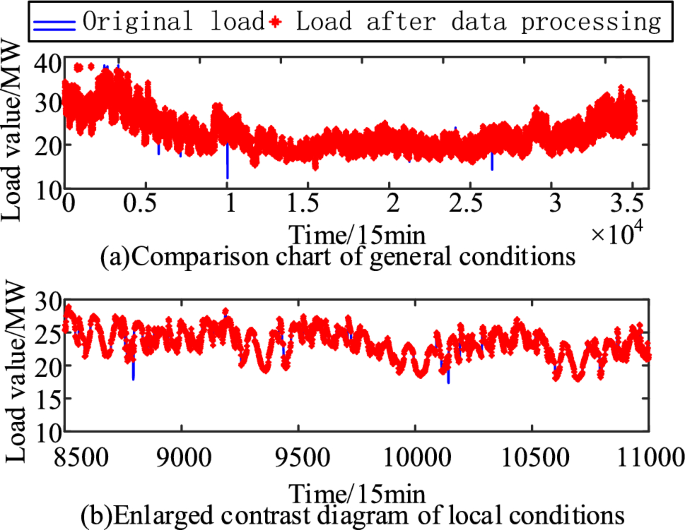
Schematic of data cleaning comparison


5.2 Data normalization
In this study, the short-term load forecasting data were normalized based on the linear normalization method. The normalized interval was [0,1], as expressed in Eq. (20):
where \({\varvec{x}}_{{{\text{nor}}}}\) is the normalized power load data sequence; x is the original power load data sequence; and \({\varvec{x}}_{\max }\) and \({\varvec{x}}_{\min }\) are the maximum and minimum values in the original power load data sequence, respectively.
5.3 FCM cluster analysis of load
In this study, the FCM method was used to cluster the load data; the process was thoroughly described in SubSect. 2.1. The daily load data from July 2019 to July 2020 as well as the corresponding historical meteorological information data and calendar rule information were used as data samples for FCM clustering. To determine the reasonable number of FCM clusters, the sum of the distance between the load curve and FCM cluster center in all classifications was recorded as \(D_{l,c}\) to investigate the similarity of the elements in the FCM cluster results.
where \(M\) is the number of cluster centers, \(S\) is the number of load curves included in the i-th load curve, \(c_{i}\) is the cluster center of the i-th class, and \(l_{i,j}\) is the j-th load curve in the i-th class.
In addition, the total distance between two clusters of all cluster centers is recorded as \(D_{c,c}\) to evaluate the degree of difference between clusters in the FCM clustering results, as expressed in Eq. (22).
Finally, the ratio of \(D_{l,c}\) and \(D_{c,c}\) is recorded as \({\text{Val}}\) to evaluate the FCM clustering results, as expressed in Eq. (23). Based on the clustering idea that the element similarity within a class is the possible maximum and the similarity between classes is the possible minimum, the ideal FCM clustering result should have a smaller \(D_{l,c}\) value, larger \(D_{c,c}\) value, and relatively smaller \({\text{Val}}\) value. The cluster number interval \([1,20]\) was selected, and the \({\text{Val}}\) value under each cluster number was calculated. The change in the \({\text{Val}}\) value of the FCM clustering evaluation index is shown in Fig. 7.

\({\text{Val}}\) evaluation index of FCM clustering
As the number of clusters gradually increases in the interval \([1,20]\), the relative distance between classes becomes larger; thus, the value of \(D_{c,c}\) increases. Simultaneously, the relative distance between load curves in each category becomes smaller; thus, the value of \(D_{l,c}\) decreases. Therefore, based on the change in \(D_{c,c}\) and \(D_{l,c}\) values, it can be observed from Fig. 7 that \({\text{Val}}\) decreases with an increasing number of clusters in the interval \([1,20]\). However, before the number of clusters is six, \({\text{Val}}\) decreases rapidly. However, after the number of clusters becomes six, the downward trend of \({\text{Val}}\) is significantly extenuated. Therefore, based on the idea of the inflection point method, the optimal number of FCM clusters is six.
Subsequently, the clustering task was carried out according to the process described in SubSect. 2.1. Figure 8 shows the FCM clustering results of the load curve. Obvious differences among various types of FCM clustering results can be seen; indeed, each type has a certain number of compact load curves. Therefore, it is reasonable to select FCM clustering results with a cluster number of six.

Load FCM clustering analysis results
5.4 Two-stage fuzzy optimization of load feature extraction
After the FCM clustering analysis of the load curve was completed, the initial feature extraction of various loads was carried out according to the DP algorithm flowchart of the fuzzy optimization threshold, as described in SubSect. 2.3.1. The threshold setting process of the DP algorithm was used for fuzzy optimization of the third type of load. Figure 9 shows the changes in average DTW matching degree \(D\left( \varepsilon \right)\), average compression ratio \(Z\left( \varepsilon \right)\), and threshold membership degree \(Sat\left( \varepsilon \right)\) during the gradual increase in DP algorithm threshold of the third type of load in the interval \([0,1]\).

Schematic of the third type of fuzzy optimization threshold of load
Figure 9 shows that the number of features extracted for the first time decreases as the threshold of the DP algorithm for the third type of load gradually increases in the interval \([0,1]\). Thus, the average compression ratio \(Z\left( \varepsilon \right)\) exhibits a gradual upward trend. Simultaneously, the fitting degree between the characteristic and original curves decreases, resulting in a gradual decline in the trend of the average DTW matching degree \(D\left( \varepsilon \right)\). Therefore, the \(Sat\left( \varepsilon \right)\) curve of threshold membership rises first and then falls. The threshold corresponding to the maximum value of the threshold membership \(Sat\left( \varepsilon \right)\) is the optimal threshold of the DP algorithm for this type of load curve cluster. Figure 9 shows that the optimal threshold value of the DP algorithm for the third type of load after the fuzzy optimization analysis is 0.2. Based on the first feature extraction, the second feature extraction of the third type of load curve cluster was carried out using the statistical frequency distribution process, as described in SubSect. 2.3.2. Figure 10 shows the final feature recognition and extraction results of the third type of load curve cluster.

Characteristic dimension diagram of the third type of load curve cluster
Figure 10 illuminates that after applying the proposed two-stage fuzzy optimization of load feature recognition and extraction, the load feature dimension of the third type of load curve cluster is simplified from the original 96–62 dimensions, and the average compression ratio is approximately 65.0%. It not only effectively simplifies part of the inputs of the combined short-term load forecasting model but also completes the feature selection and dimension reduction. Therefore, the important original shape feature information of the load curve is retained, which provides a reliable supporting condition for the accurate prediction of the subsequent combined short-term load forecasting model.
5.5 Evaluation of the model performance
The performance evaluation indicators of the forecasting model were the relative error rate \(E_{i}\) at load forecasting point \(i\), root-mean-square error \(E_{{{\text{RMSE}}}}\) of the overall load forecasting, average absolute percentage error rate \(E_{{\text{MAPE}}}\), and overall forecasting accuracy rate \({\text{Acc}}\), as expressed in Eqs. (24–27).
where \(\hat{x}_{i}\) and \(x_{i}\) are the predicted and actual values of power load at point \(i\), respectively.
5.6 Results and discussion
5.6.1 Load characteristic prediction
The load of the prediction calculation system on August 1, 2020, is taken as an example. The maximum transfer probability state calculated by the probability matrix of the Markov chain model in Sect. 2.2 combined with the historical state indicates that the daily load most likely belongs to the third type of the load curve cluster. Thus, the third type of load characteristics and its influencing factors should be used as the source of training samples on that day. At present, the parameter setting of the neural network and support vector machine has not formed a complete theory to guide. The parameter value interval in the neural network is determined empirically, and specific parameters are set using experiments and comparisons [23, 24]. The optimal parameters of the SVM model are determined based on grid search and cross-validation [25]. Because a three-layer neural network can approximate any complex continuous nonlinear function [26], the number of layers of the neural network was selected as three, and the hidden layer neurons of the NARX neural network were set for parameter trial optimization, as shown in Fig. 11.

Optimal setting of hidden layer neurons
Figure 11 shows that the optimal interval for trial based on an empirical equation is [11, 20]. To avoid the contingency of a single test, 10 rounds of calculation were conducted for the number of neurons in each hidden layer, and the mean square error of repeated test training data samples was calculated. When the number of neurons in the hidden layer was 18, because the mean square error of each round of training data sample test error was at a low level and its mean value reached the minimum value; the exploratory optimization process was used to determine the number of neurons in the hidden layer of the NARX neural network, which was finally regarded as 18. Table 1 lists the key parameter settings of the proposed model after exploratory optimization and search verification.
As shown in Fig. 12, based on the fuzzy clustering analysis, the FCM-TFIDP-BP, FCM-TFIDP-SVM, and FCM-TFIDP-NARX composite models were, respectively, constructed using the proposed two-stage fuzzy optimization of load feature recognition and extraction method, BP neural network, SVM, and NARX neural network through cascade settings.

Prediction results of load characteristics
Figure 12 shows that, compared with the typical BP neural network and SVM structure, the cyclic NARX neural network with time-delay feedback connection can better mine the correlation characteristics between the load characteristic sequences with complex nonlinearity; thus, this network has the best overall prediction effect of load characteristics. Table 2 summarizes a comparison between the load feature prediction results of FCM-TFIDP-BP, FCM-TFIDP-SVM, and FCM-TFIDP-NARX models. The evaluation indicators are ERMSE and EMAPE of load feature prediction.
Table 2 shows that the ERMSE of FCM-TFIDP-NARX is 1.028 MW and its EMAPE is 3.484%; these values are better than those of FCM-TFIDP-BP and FCM-TFIDP-SVM. Accurate load characteristics provide a decisive foundation for the subsequent improvement of the overall short-term load forecasting accuracy.
5.6.2 Evaluation of short-term load forecast
As shown in Fig. 13, based on the BP neural network, SVM, and NARX neural network, the direct method, the simple load feature recognition combined forecasting model with a fixed threshold of 0.5, and the fuzzy optimization load feature recognition combined forecasting model were used to compare the short-term load forecasting results of the case study for 3 consecutive days from August 1 to August 3, 2020. Moreover, the predicted load characteristics were reconstructed to the original dimensions based on the SP fitting technology.

Prediction results of load characteristics
Table 3 lists a summary of the indicators to evaluate the prediction performance of the proposed model. The evaluation indicators include ERMSE, EMAPE, Acc, and the total calculation time of the short-term load forecasting on working and rest days. According to Fig. 13 and Table 3, obtaining reasonable results for short-term load forecasting based on a single machine learning forecasting model is difficult. In the process of continuous short-term load forecasting, the ERMSE of the BP neural network on working and rest days reached 4.243 and 4.524 MW, respectively, owing to the problems of easily falling into local minimum points and “overfitting.” However, EMAPE reached 12.969 and 13.485%, respectively, and the prediction effect was poor. Moreover, the typical SVM model exhibited an insufficient training generalization ability for massive data samples; hence, its prediction performance cannot fulfill the actual demand. However, the NARX neural network exhibited the highest overall prediction performance based on the advantages of its own cyclic delay feedback structure. Indeed, ERMSE and EMAPE of the NARX neural network are the lowest among the comparison single machine learning forecasting models. However, owing to the complex nonlinear effects of load fluctuation and influencing factors, the NARX neural network yields large prediction errors at some load characteristic prediction points. Therefore, the overall prediction accuracy must be improved.
Figure 13 and Table 3 reveal that the proposed load feature recognition forecasting model improves the overall forecasting accuracy compared with the single machine learning forecasting models because it forecasts the load features with more details and uses an appropriate SP fitting technology for load reconstruction. Furthermore, the ERMSE of FCM-DP-BP on a week and rest days decreased by 0.942 and 0.775 MW, respectively, compared with that of FCM-BP. In addition, EMAPE decreased by 2.408 and 1.113%, respectively. Similarly, the Acc of FCM-DP-SVM in a week and rest days increased by 1.626 and 1.160%, respectively, compared with that of FCM-SVM. Furthermore, Acc of FCM-DP-NARX is 0.545 and 0.433% higher than that of FCM-NARX. Therefore, the combined forecasting model of load characteristics recognition with a fixed pattern is completely practical.
This study proposed an adaptive improved fuzzy optimization load feature recognition combined forecasting model to alleviate the limitations of the fixed-pattern load feature recognition combined forecasting model and further improve the accuracy of load forecasting. Compared with the fixed-pattern load feature recognition combined forecasting model, the fuzzy optimization load feature recognition combined forecasting model is more sensitive to load feature prediction. Moreover, the adaptive two-stage fuzzy optimization method for load feature identification and extraction can effectively analyze the necessary load feature set to provide support for accurate prediction of future load features. In addition, the load feature dimension considered by the combined fuzzy optimization load feature recognition model is more reasonable than the combined load feature recognition model with a fixed pattern. Therefore, it not only supports the forecasting model to efficiently mine the correlation characteristics between load characteristics and improve the accuracy of load characteristics forecasting but also enhances the rationality and effectiveness of load fitting and reconstruction, and thus effectively improves the final load forecasting accuracy. Moreover, according to the total calculation time statistics listed in Table 3, compared with the single machine learning prediction model, the fixed-mode load feature recognition and fuzzy optimization load feature recognition combined forecasting models focus on the load characteristics. The input scale of the model can be clearly and effectively reduced; thus, the computational efficiency is improved. However, the calculation time of the fuzzy optimization load feature recognition combined forecasting model is higher than that of the fixed-mode load feature recognition combined forecasting model because of its more refined load feature mining. Therefore, the combined forecasting model of fuzzy optimization load feature recognition can obtain a higher load forecasting accuracy at a reasonable calculation time. Among them, the FCM-TFIDP-NARX combined forecasting model exhibits the highest performance and satisfactorily combines the superior structural performance of the NARX neural network for nonlinear time-series problems using cyclic delay feedback structure and practical application advantages of adaptive two-stage fuzzy optimization of load feature recognition. ERMSE on rest days is only 1.101 MW, EMAPE is 3.200%, whereas ERMSE on weekdays is 1.073 MW, and EMAPE is only 3.587%. The overall prediction accuracy is 95.914%, and the calculation time is approximately 48% less than that of FCM-NARX. It not only significantly reduces the computational complexity of the combined forecasting model but also effectively improves the accuracy of short-term load forecasting results, which can reliably meet the targeted demand under the new development background.
6 Conclusions
Based on a typical machine learning forecasting framework, this study introduced a combined forecasting model of fuzzy optimization load feature recognition. Additionally, the proposed model was applied to an actual case study to validate its short-term load forecasting performance. Based on the theoretical analysis and verification of the calculation results, the following conclusions were obtained:
-
(1)
Advanced Performance of NARX Neural Network: Our comparison of traditional machine learning models such as BP neural networks and SVM support vector machines with the NARX neural network demonstrates the superior performance of the latter. The recurrent delayed feedback structure of the NARX network allows for better capture of dynamic load sequence characteristics, leading to enhanced predictive performance. Future work will involve further optimization and fine-tuning of the NARX network architecture to maximize its potential in load forecasting applications.
-
(2)
Refinement in Load Characteristic Identification Combination Forecasting Model: Our study highlights the advantages of the load characteristic identification combination forecasting model over single machine learning prediction models. The model offers a finer prediction of load characteristics and load reconstruction processes, resulting in overall improved predictive performance. Future research will focus on exploring additional features and refining the model parameters to further enhance its accuracy and reliability.
-
(3)
Integration of Adaptive Improvements: The incorporation of adaptive improvements based on fixed-pattern load characteristic identification combination forecasting models into the fuzzy optimization load characteristic identification combination forecasting model represents a significant advancement. By adapting to changes in load patterns and characteristics, the model can better capture the precise features of loads, thereby enhancing overall predictive accuracy. Future work will involve continuous monitoring and updating of the model to ensure its adaptability to evolving load dynamics.
In the context of evolving developments in the power system, our proposed fuzzy optimization load characteristic identification combination forecasting model addresses various targeted needs of load forecasting and holds practical research value. Future research directions include exploring how to effectively describe the coupling transformation characteristics among various complex loads and incorporating these insights to further improve the model.
References
Wang X, Wang Q (2019) A short-term load forecasting method based on fuzzy neural RBF network adaptive control. IOP Conf. Ser. Mater. Sci. Eng. 490(4):042041. https://doi.org/10.1088/1757-899X/490/4/042041
Yavuz E, İbrahim K (2024) A comprehensive review on deep learning approaches for short-term load forecasting. Renew Sustain Energy Rev 189(10):114031. https://doi.org/10.1016/j.rser.2023.114031
Majid M, Altug B, Yavuz A (2023) Load forecasting based on genetic algorithm-artificial neural network-adaptive neuro-fuzzy inference systems: a case study in Iraq. Energies 16(6):2919–2919. https://doi.org/10.3390/en16062919
Zhu L (2022) Market-based versus price-based optimal trading mechanism design in microgrid. Comput Electr Eng 100:107904. https://doi.org/10.1016/j.compeleceng.2022.107904
Sorknæs P et al (2020) Smart energy markets-future electricity, gas and heating markets. Renew Sust Energ Rev 119(5):109655. https://doi.org/10.1016/j.rser.2019.109655
Karaki SH (1999) Weather sensitive short-term load forecasting using artificial neural networks and time series. Int J Electr Power Energy Syst 19(3):251–256
Xue W (2022) Power system short-term load forecasting based on BP neural network. J Phys: Conf Ser 2378(1):012007
Singh P, Dwivedi P, Kant V (2019) A hybrid method based on neural network and improved environmental adaptation method using Controlled Gaussian Mutation with real parameter for short-term load forecasting. Energy 174:460–477. https://doi.org/10.1016/j.energy.2019.02.141
Yang Y, Che J, Deng C et al (2019) Sequential grid approach based support vector regression for short-term electric load forecasting. Appl Energy 238:1010–1021. https://doi.org/10.1016/j.apenergy.2019.01.127
Boudet HS, Flora JA, Armel KC (2016) Clustering household energy-saving behaviours by behavioural attribute. Energy Policy 92:444–454. https://doi.org/10.1016/j.enpol.2016.02.033
Liu X, Zhang Z, Song Z (2020) A comparative study of the data-driven day-ahead hourly provincial load forecasting methods: from classical data mining to deep learning. Renew Sust Energ Rev 119(C):109632. https://doi.org/10.1016/j.rser.2019.109632
Chen J, Li T, Zou Y et al. (2019) An ensemble feature selection method for short-term electrical load forecasting. In: 2019 IEEE 3rd Conference on Energy Internet and Energy System Integration (EI2), 1429–1432
Salami M, Sobhani FM, Ghazizadeh MS (2019) A hybrid short-term load forecasting model developed by factor and feature selection algorithms using improved grasshopper optimization algorithm and principal component analysis. Electr Eng 102:1–24. https://doi.org/10.1007/s00202-019-00886-7
Yahaya AS, Javaid N, Latif K et al. (2019) An enhanced very short-term load forecasting scheme based on activation function. In: 2019 International Conference on Computer and Information Sciences (ICCIS), 1–6
Alfian B, Hapsari HH, Fuad RR (2023) Extraction of road network in urban area from orthophoto using deep learning and douglas-peucker post-processing algorithm. IOP Conference Series: Earth and Environmental Science, 1127(1)
Jasim KA, Tanha J, Balafar AM (2024) Neighborhood information based semi-supervised fuzzy C-means employing feature-weight and cluster-weight learning. Chaos Solitons Fractals: Interdiscip J Nonlinear Sci Nonequilib Complex Phenom 181:114670. https://doi.org/10.1016/j.chaos.2024.114670
Hu Z, Fang J, Zheng R et al (2024) Efficient model predictive control of boiler coal combustion based on NARX neutral network. J Process Control 134:103158. https://doi.org/10.1016/j.jprocont.2023.103158
Alhakeem ZM, Rashid MT (2023) Electric vehicle battery states estimation during charging process by NARX neural network. J Control Autom Electr Syst 34(6):1194–1206
Fabio ND, Francesco G, Rudy G et al (2021) Prediction of spring flows using nonlinear autoregressive exogenous (NARX) neural network models. Environ Monitor Assess 193(6):350–350
Huang JJ, Chen YC (2024) Integrating the coupled markov chain and fuzzy analytic hierarchy process model for dynamic decision making. Axioms 13(2):95. https://doi.org/10.3390/axioms13020095
Budi L, Nur C et al (2023) Determining confidence interval and asymptotic distribution for parameters of multi-response semiparametric regression model using smoothing spline estimator. J King Saud Univ - Sci 35(5):102664
Zhang Y, Shen H, Ma J (2018) Load characteristic analysis and application research on integrated energy system. Electr Power Constr 39(09):18–29
Xiao B, Xiao Z, Jiang Z et al (2021) Spatial load situation awareness based on denoising autoencoder, singular spectrum analysis and long short-term memory neural networks. Proc CSEE 41(14):4858–4867
Pang H, Gao J, Du Y (2020) A short-term load probability density prediction based on quantile regression of time convolution network. Power Syst Technol 44(04):1343–1350
Xi Y, Wu J, Shi C et al (2019) A refined load forecasting based on historical data and real-time influencing factors. Power Syst Prot Control 47(01):80–87
Wang L, Mendel JM (1992) Fuzzy basis functions, universal approximation, and orthogonal least-squares learning. IEEE Trans Neural Netw 3(5):807–814. https://doi.org/10.1109/72.159070
Acknowledgements
This paper is supported by the Science and Technology Program of China Southern Power Grid Co., Ltd. (Grant No. YNKJXM20222178), the Reserve Talents Program for Middle-aged and Young Leaders of Disciplines in Science and Technology of Yunnan Province, China (Grant No. 202105AC160014), and Guangdong Basic and Applied Basic Research Foundation (2022A1515240074).
Author information
Authors and Affiliations
Contributions
Shengzhen Lin and Yuxing Xie have written the main manuscript text, and all other authors, including Yigong Xie, Xinchun Zhu, Yang Wu, Shuangquan Liu, and Min Xie, have reviewed the manuscript.
Corresponding author
Ethics declarations
Conflict of interest
The authors have no conflicts.
Additional information
Publisher's Note
Springer Nature remains neutral with regard to jurisdictional claims in published maps and institutional affiliations.
Rights and permissions
Open Access This article is licensed under a Creative Commons Attribution 4.0 International License, which permits use, sharing, adaptation, distribution and reproduction in any medium or format, as long as you give appropriate credit to the original author(s) and the source, provide a link to the Creative Commons licence, and indicate if changes were made. The images or other third party material in this article are included in the article's Creative Commons licence, unless indicated otherwise in a credit line to the material. If material is not included in the article's Creative Commons licence and your intended use is not permitted by statutory regulation or exceeds the permitted use, you will need to obtain permission directly from the copyright holder. To view a copy of this licence, visit http://creativecommons.org/licenses/by/4.0/.
About this article

Cite this article
Xie, Y., Zhu, X., Wu, Y. et al. Short-term load forecasting method based on fuzzy optimization combined model of load feature recognition. Electr Eng (2024). https://doi.org/10.1007/s00202-024-02539-w
Received:
Accepted:
Published:
DOI: https://doi.org/10.1007/s00202-024-02539-w