Detection-only versus detection and identification of model misspecifications

Abstract

It is common practice to use the well-known concept of the minimal detectable bias (MDB) to assess the performance of statistical testing procedures. However, such procedures are usually applied to a null and a set of multiple alternative hypotheses with the aim of selecting the most likely one. Therefore, in the DIA method for the detection, identification and adaptation of model misspecifications, rejection of the null hypothesis is followed by identification of the potential source of the model misspecification. With identification included, the MDBs do not truly reflect the capability of the testing procedure and should therefore be replaced by the minimal identifiable bias (MIB). In this contribution, we analyse the MDB and the MIB, highlight their differences, and describe their impact on the nonlinear DIA-estimator of the model parameters. As the DIA-estimator inherits all the probabilistic properties of the testing procedure, the differences in the MDB and MIB propagation will also reveal the different consequences a detection-only approach has versus a detection+identification approach. Numerical algorithms are presented for computing the MDB and the MIB and also their effect on the DIA-estimator. These algorithms are then applied to a number of examples so as to analyse and illustrate the different concepts.

1 Introduction

Empirical data are often collected to make statistical inferences about a certain phenomenon. In doing so, a set of candidate observational models are considered that could potentially describe the observed phenomenon. An inference procedure will then often involve, on the basis of the collected data, selecting the most likely model among the hypothesized ones through a testing procedure, and estimating the unknown parameters of interest based on the identified model. This combined estimation and testing process is captured in the DIA-method for the detection, identification and adaptation of model misspecifications (Teunissen 2018). Although the method was initially developed for geodetic quality control (Baarda 1968; Teunissen 1985), it also found successful applications in other fields, including navigational integrity (Teunissen 1990; Gillissen and Elema 1996; Yang et al. 2014), deformation analysis and structural health monitoring (Verhoef and De Heus 1995; Yavaşoğlu et al. 2018; Durdag et al. 2018; Lehmann and Lösler 2017; Nowel 2020), and GNSS integrity monitoring (Jonkman and De Jong 2000; Kuusniemi et al. 2004; Hewitson and Wang 2006; Khodabandeh and Teunissen 2016).

For a proper probabilistic evaluation, it is crucial that all uncertainties of detection, identification and adaptation are accounted for when describing the quality of the finally produced output. In the Detection step, the validity of the null hypothesis (working model) $\mathcal {H}_{0}$ is checked. If $\mathcal {H}_{0}$ is rejected in the detection step, the Identification step is taken so as to select the most likely alternative hypothesis among the candidate ones. The Adaptation step is then followed to correct earlier $\mathcal {H}_{0}$-based inferences according to the decision made in the identification step. Therefore, in the DIA procedure, estimation of the unknown parameters is always affected by the outcome of testing of the considered hypotheses through detection and identification steps. As the finally produced DIA-estimator will then have inherited all uncertainties stemming from both estimation and testing, it is its probability density function (PDF) that should form the basis of any qualitative analysis (Teunissen 2018).

In this contribution, we study the multi-hypothesis testing performance of the detection and identification steps using the concepts of the minimal detectable bias (MDB) (Baarda 1967, 1968) and the minimal identifiable bias (MIB) (Teunissen 2018), respectively. The former is a diagnostic tool for measuring the ability of the testing procedure to detect misspecifications of the model, while the latter is a diagnostic tool for measuring the ability of the testing procedure to correctly identify misspecifications of the model. The difference between the MDB and the MIB has already been studied for outlier detection and identification in (Imparato et al. 2019; Zaminpardaz and Teunissen 2019). In this contribution, we analyse and demonstrate the difference between the MDB and the MIB for higher-dimensional biases, whereby for identification all test statistics are transformed to have a common distribution so as to take their differences in degrees of freedom into account. Furthermore, we show how the MDB- and MIB-sized bias get propagated into the DIA-estimator for detection-only and detection+identification testing regimes, respectively. Next to the provided theory, we also provide computational procedures on how to compute the MDB, the MIB and their propagation into the mean of the nonlinear DIA-estimator.

This contribution is structured as follows. A brief review of the DIA method is provided in Sect. 2. We specify the null and alternative hypotheses and discuss the implementation of the testing and estimation schemes of the DIA method using a canonical model formulation and a partitioning of misclosure space. The testing decisions and their probabilities are discussed, leading to the DIA-estimator, for which the statistical distribution and mean are then provided. It is thereby highlighted that the DIA-estimator is always biased under the alternative hypotheses, and we show how its bias can be numerically evaluated.

In Sect. 3, we specify the detection test, discuss its MDB and provide a numerical algorithm for the MDB computation. In Sect. 4, we formulate the identification test for the general situation where the alternative hypotheses are of multiple dimensions and different from each other. The corresponding MIB together with a numerical algorithm for its computation are then provided and discussed. Section 5 provides, by means of a number of examples, an analysis of the MDBs and the MIBs, their differences and their impact on the DIA-estimator. To emphasize the difference between the concepts of the MDB and the MIB, we hereby discriminate between two testing schemes: (1) Detection-only and (2) Detection+Identification. In the detection-only case, the MDB shows the minimal size of biases that lead to the rejection of $\mathcal {H}_0$, and thus to an unavailability of a parameter solution. To avoid such unavailability, one can include identification at the expense of a larger risk. In the detection+identification case, the MIB shows the minimal size of biases that can be identified. It is highlighted that using MDB to infer the identifiability of alternative hypotheses is dangerous as it could lead to misleading conclusions on the testing performance. Finally, a summary with conclusions is provided in Sect. 6.

We use the following notation: $\textsf{E}(\cdot )$ and $\textsf{D}(\cdot )$ denote the expectation and dispersion operator, respectively. The space of all n-dimensional vectors with real entries is denoted as $\mathbb {R}^{n}$, while the zero-centred sphere $\mathbb {S}^{n-1}\subset \mathbb {R}^{n}$ contains the unit n-vectors from origin. Random vectors are indicated by use of the underlined symbol ‘$\underline{\cdot }$’. Thus, $\underline{y} \in \mathbb {R}^{m}$ is a random vector, while y is not. The squared weighted norm of a vector, with respect to a positive-definite matrix Q, is defined as $\Vert \cdot \Vert ^{2}_{Q}=(\cdot )^{T}Q^{-1}(\cdot )$. $\mathcal {H}$ is reserved for statistical hypotheses, $\mathcal {P}$ for regions partitioning the misclosure space, $\mathcal {N}(y,Q)$ for the normal distribution with mean y and variance matrix Q, and $\chi ^{2}(r,\lambda ^{2})$ for the Chi-square distribution with r degrees of freedom and the non-centrality parameter $\lambda ^{2}$. The cumulative distribution function (CDF) of the distribution $*$ is shown by CDF$_{*}(\cdot )$. $\textsf{P}(\cdot )$ denotes the probability of the occurrence of the event within parentheses. The symbol $\overset{\mathcal {H}}{\sim }$ should be read as ‘distributed as $\ldots$ under $\mathcal {H}$’. The superscripts $^{T}$ and $^{-1}$ are used to denote the transpose and the inverse of a matrix, respectively.

2 An overview of the DIA method

In this section, we provide a brief overview of the DIA method and describe its testing and estimation elements. As our point of departure, we first formulate the null- and alternative hypotheses, where we restrict our attention to the linear model with normally distributed observables, which is commonly used in different applications. Under the null hypothesis $\mathcal {H}_{0}$, the random vector of observables $\underline{y}\in \mathbb {R}^{m}$ is assumed to be normally distributed as

$$\begin{aligned} \mathcal {H}_{0}:\quad \underline{y}\;{\sim }\;\mathcal {N}\left( Ax~,~Q_{yy}\right) \end{aligned}$$

(1)

where its mean is linearly parameterized in the unknown parameters $x\in \mathbb {R}^{n}$ through the known full-rank design matrix $A\in \mathbb {R}^{m\times n}$, and its dispersion is modelled by the positive-definite variance matrix $Q_{yy}\in \mathbb {R}^{m\times m}$. The best linear unbiased estimator (BLUE) of x based on (1) is given as

$$\begin{aligned} \hat{\underline{x}}_{0}\;=\;A^{+}\,\underline{y} \end{aligned}$$

(2)

in which $A^{+}=(A^{T}Q_{yy}^{-1}A)^{-1}A^{T}Q_{yy}^{-1}$ is the BLUE-inverse of A.

When modelling $\underline{y}$ through (1), different types of misspecifications could be expected, including $\textsf{E}(\underline{y})\;\ne \;Ax$, $\textsf{D}(\underline{y})\;\ne \;Q_{yy}$, and $\underline{y}$ not following a normal distribution. Here, we assume that a misspecification is restricted to an underparametrization of the mean of $\underline{y}$ (Teunissen 2017). Hence, the alternative hypothesis $\mathcal {H}_{i}$ takes the form

$$\begin{aligned} \mathcal {H}_{i}:\quad \underline{y}\;{\sim }\;\mathcal {N}(Ax\,+\,\underbrace{C_{i}b_{i}}_{b_{y_i}}~,~Q_{yy}) \end{aligned}$$

(3)

for some vector $b_{y_{i}}=C_{i}b_{i}\in \mathbb {R}^{m}\setminus \{0\}$ such that $[A~~C_{i}]\in \mathbb {R}^{m\times (n+q_{i})}$ is a known matrix of full rank and $b_i\in \mathbb {R}^{q_{i}}$ is an unknown bias vector. The BLUE of x based on (3) is not given by (2), but instead by

$$\begin{aligned} \hat{\underline{x}}_{i}\;=\;\bar{A}_{i}^{+}\,\underline{y} \end{aligned}$$

(4)

where $\bar{A}_{i}^{+}=(\bar{A}_{i}^{T}Q_{yy}^{-1}\bar{A}_{i})^{-1}\bar{A}_{i}^{T}Q_{yy}^{-1}$ is the BLUE-inverse of $\bar{A}_{i}=P^{\perp }_{C_{i}}A$, with $P^{\perp }_{C_{i}}=I_{m}-P_{C_{i}}$ and $P_{C_{i}}=C_{i}(C_{i}^{T}Q_{yy}^{-1}C_{i})^{-1}C_{i}^{T}Q_{yy}^{-1}$ being the orthogonal projector that projects onto the range space of $C_{i}$. As, in practice, there are several different sources that can make the observables’ mean deviate from the $\mathcal {H}_0$-model, multiple alternative hypotheses usually need to be considered to capture the corresponding deviations. For example when modelling GNSS data, one may need to take into account pseudorange outliers, carrier-phase cycle slips and non-negligible atmospheric delays. In the following, we assume that there are $k\ge 1$ alternative hypotheses of the form of (3).

Having specified the null and alternative hypotheses, the DIA procedure is carried out using a sample of observables $\underline{y}$ as follows (Baarda 1968; Teunissen 1985):

• Detection: The assumed null hypothesis $\mathcal {H}_0$ undergoes a validity check for the observed data, without the need of having to consider a particular set of alternative hypotheses. If $\mathcal {H}_{0}$ is decided to be valid, $\hat{\underline{x}}_{0}$ is provided as the estimator of x.

• Identification: In case $\mathcal {H}_{0}$ is decided to be invalid in the detection step, a search is carried out among the specified alternatives $\mathcal {H}_{i}$ ($i = 1,\ldots ,k$) to pinpoint the discrepancy between $\mathcal {H}_{0}$ and the observed data. In doing so, two decisions can be made. Either one of the alternative hypotheses, say $\mathcal {H}_{i}$, is confidently identified, or none can be identified as such in which case an ‘undecided’ decision is made.

• Adaptation: If $\mathcal {H}_{i}$ is confidently identified, it takes the role of the new null hypothesis, and thus $\hat{\underline{x}}_{i}$ is provided as the estimator of x. However, in case the ‘undecided’ decision is made, then the solution for x is declared ‘unavailable’.

2.1 Implementation of the DIA method

Let $B\in \mathbb {R}^{m\times r}$, with $r=m-n$ the redundancy under $\mathcal {H}_{0}$, be a basis matrix of the null space of $A^{T}$, i.e. $A^{T}B=0$ and rank $(B)=r$. The random vector of observables $\underline{y}$ can be brought in canonical form using one-to-one Tienstra-transformation $\mathcal {T}=[A^{+^{T}},~B^{T}]^{T}\in \mathbb {R}^{m\times m}$ as (Tienstra 1956; Teunissen 2018)

$$\begin{aligned} \mathcal {T}\underline{y}= \left[ \begin{array}{c}\underline{\hat{x}}_{0}\\ \underline{t}\end{array} \right] \left\{ \begin{array}{l} \overset{\mathcal {H}_{0}}{\sim }\mathcal {N}\left( \left[ \begin{array}{c}x\\ 0 \end{array}\right] ,\left[ \begin{array}{cc}Q_{\hat{x}_{0}\hat{x}_{0}}&{}0\\ 0&{}Q_{tt}\end{array}\right] \right) \\ \overset{\mathcal {H}_{i}}{\sim }\mathcal {N}\left( \left[ \begin{array}{c}x+b_{\hat{x}_{0,i}} \\ b_{t_{i}}\end{array}\right] ,\left[ \begin{array}{cc}Q_{\hat{x}_{0}\hat{x}_{0}}&{}0\\ 0&{}Q_{tt} \end{array}\right] \right) \end{array} \right. \end{aligned}$$

(5)

where $\underline{t}\in \mathbb {R}^{r}$ is the vector of misclosures, and

$$\begin{aligned} \begin{array}{lll} b_{\hat{x}_{0,i}}=A^{+}b_{y_i}&{},&{}Q_{\hat{x}_{0}\hat{x}_{0}}=(A^{T}Q^{-1}_{yy}A)^{-1} \\ b_{t_{i}}=B^{T}b_{y_i}&{},&{}Q_{tt}=B^{T}Q_{yy}B \end{array} \end{aligned}$$

(6)

As $\underline{t}$ has a known PDF under $\mathcal {H}_{0}$, which is the PDF of $\mathcal {N}(0, Q_{tt})$, and is independent of $\underline{\hat{x}}_{0}$, any statistical testing procedure is driven by the misclosure vector and its known PDF under $\mathcal {H}_{0}$. Therefore, it is the component $b_{t_{i}}$ of $b_{y_i}$ that is testable. The component $b_{\hat{x}_{0,i}}$ of $b_{y_i}$ however is influential as it is directly absorbed by the parameter vector (Baarda 1967, 1968; Teunissen 2006).

As shown by Teunissen (2018), any testing procedure can be translated into a partitioning of the misclosure space $\mathbb {R}^{r}$. Let $\mathcal {P}_{i}\subset \mathbb {R}^{r}$ ($i=0,1,\ldots ,k,k+1$) be a partitioning of the misclosure space, i.e. $\bigcup _{i=0}^{k+1}\,\mathcal {P}_{i}=\mathbb {R}^{r}$ and $\mathcal {P}_{i}\cap \mathcal {P}_{j}=\emptyset$ for $i\ne j$. The testing procedure implied by the above detection and identification steps is then defined as

$$\begin{aligned} \begin{array}{lll} `\textrm{select}~\mathcal {H}_{i}{\text '}&{}\mathrm{if~and~only~if}&{}\underline{t}\in \mathcal {P}_{i}\quad \textrm{for}~ i=0,1\ldots ,k\\ \mathrm{`undecided\text '}&{}\mathrm{if~and~only~if}&{}\underline{t}\in \mathcal {P}_{k+1} \end{array} \end{aligned}$$

(7)

Fig. 1

An overview of testing decisions, driven by the misclosure vector $\underline{t}$, under null and alternative hypotheses (cf. 7)

where $\mathcal {P}_{k+1}$ is the undecided region for which the solution for x is declared ‘unavailable’. This undecided region could be due to weak discrimination between some of the hypotheses, unconvincing selection or accommodating the alternative hypotheses that may have been missed. In addition, the misclosure vector establishes the following link between BLUEs of x under $\mathcal {H}_{0}$ and $\mathcal {H}_{i}$ ($i=1,\ldots ,k$)

$$\begin{aligned} \hat{\underline{x}}_{i}=\hat{\underline{x}}_{0}-L_{i}\,\underline{t} \end{aligned}$$

(8)

with

$$\begin{aligned} L_{i}=A^{+}C_{i}C_{t_{i}}^{+}, \end{aligned}$$

(9)

in which $C_{t_{i}}^{+}=(C_{t_{i}}^{T}Q_{tt}^{-1}C_{t_{i}})^{-1}C_{t_{i}}^{T}Q_{tt}^{-1}$ and $C_{t_{i}}=B^{T}C_{i}$. Therefore, implementation of the three DIA steps requires nonzero redundancy under $\mathcal {H}_{0}$, i.e. $r=m-n\ne 0$, so that misclosures can be formed. Note, in single-redundancy case $r = 1$, that $\mathcal {P}_{1}=\ldots =\mathcal {P}_{k}=\mathbb {R}^{r}\setminus (\mathcal {P}_{0}\cup \mathcal {P}_{k+1})$, implying that the alternative hypotheses are not distinguishable from one another, and thus identification would not be possible.

Note that the condition $\mathcal {P}_{i}\cap \mathcal {P}_{j}=\emptyset$ for $i\ne j$ is considered for the interior points of the distinct regions $\mathcal {P}_{i}$’s ($i=0,1,\ldots ,k,k+1$). These regions are allowed to have common boundaries since we assume the probability of $\underline{t}$ lying on one of the boundaries to be zero. We also note, although in (7), statistical testing is formulated in the misclosure vector $\underline{t}$, that one can equally well work with the least-squares residual vector $\hat{\underline{e}}_{0}=\underline{y}-A\hat{\underline{x}}_{0}$. By using the relation $\underline{t}=B^{T}\hat{\underline{e}}_{0}$, there is no explicit need of having to compute $\underline{t}$ as testing can be expressed directly in $\hat{\underline{e}}_{0}$ (Teunissen 2006).

Table 1 Probability of the occurrence of the events in Fig. 1

2.2 Testing decisions

As (7) shows, the testing decisions are driven by the outcome of the misclosure vector $\underline{t}$. Under each hypothesis $\mathcal {H}_{i}$ ($i=0,1,\ldots ,k$), the outcome of $\underline{t}$ can lead to $k+2$ different decisions out of which only one is correct, i.e. when $\underline{t}\in \mathcal {P}_{i}$. With $k+1$ hypotheses $\mathcal {H}_{i}$’s ($i=0,1,\ldots ,k$), one can define different statistical events including correct acceptance (CA), false alarm (FA), missed detection (MD), correct detection (CD), correct identification (CI), wrong identification (WI) and undecided (UD). The definitions of these events together with their links are illustrated in Fig. 1. In this figure, the events under alternative hypotheses are given an identifying index, as they differ from alternative to alternative. In addition, the contributions of different alternative hypotheses to the events of false alarm and wrong identification are distinguished by means of an extra index.

Given the translational property of the PDF of $\underline{t}$ under the null and alternative hypotheses (cf. 5), the probabilities of the events in Fig. 1 can be computed based on the misclosure PDF under $\mathcal {H}_{0}$, denoted by $f_{\underline{t}}(\tau |\mathcal {H}_{0})$, as shown in Table 1. These probabilities satisfy

$$\begin{aligned} \begin{array}{llllllllllllllllll} {\mathsf P}_\textrm{FA}&{}+&{}{\mathsf P}_\textrm{CA}&{}=&{}1\\ {\mathsf P}_{\textrm{CD}_{i}}(b_i)&{}+&{}{\mathsf P}_{\textrm{MD}_{i}}(b_i)&{}=&{}1\\ {\mathsf P}_{\textrm{CI}_{i}}(b_i)&{}+&{}{\mathsf P}_{\textrm{WI}_{i}}(b_i)&{}+&{}{\mathsf P}_{\textrm{UD}_{i}}(b_i)&{}=&{}{\mathsf P}_{\textrm{CD}_{i}}(b_i) \end{array} \end{aligned}$$

(10)

The probability of false alarm $\textsf{P}_\textrm{FA}$ is usually set a priori by the user. To evaluate the probabilities under $\mathcal {H}_{i}$, one needs to set the unknown bias $b_{i}$. Here, it is important to note the difference between the probabilities of correct detection and correct identification, i.e. ${\mathsf P}_{\textrm{CD}_{i}}\ge {\mathsf P}_{\textrm{CI}_{i}}$. These two probabilities would be identical if there is only one alternative hypothesis, say $\mathcal {H}_{i}$, and no undecided region since then $\mathcal {P}_{i}=\mathbb {R}^{r}\setminus \mathcal {P}_{0}$. Similar to the CD- and CI-probability, we have the concepts of the minimal detectable bias (MDB) (Baarda 1968) and the minimal identifiable bias (MIB) (Teunissen 2018). In the following sections, we highlight the difference between the MDB (${\mathsf P}_{\textrm{CD}_{i}}$) and the MIB (${\mathsf P}_{\textrm{CI}_{i}}$).

2.3 DIA-estimator

Once testing is exercised in accordance with (7), the solution for x is either given by $\underline{\hat{x}}_{i}$ if $\mathcal {H}_{i}$ is selected or declared ‘unavailable’ if an ‘undecided’ decision is made by the testing regime. The choice of an estimator for x is thus driven by the testing procedure implying that testing and estimation should not be treated separately. The concept of the DIA-estimator which captures the whole estimation-testing scheme was first introduced in (Teunissen 2018). Let $\vartheta =F^{T}x\in \mathbb {R}^{p}$ contain linear functions of x which are of interest, then $\underline{\hat{\vartheta }}_{i}=F^{T}\underline{\hat{x}}_{i}$ is the BLUE of $\vartheta$ under the $\mathcal {H}_{i}$-model ($i=0,1,\ldots ,k$). With (7), the DIA-estimator of $\vartheta$ is defined as

$$\begin{aligned} \underline{\tilde{\vartheta }}\;=\left\{ \begin{array}{ll}\displaystyle \sum \limits _{i=0}^{k}\;\underline{\hat{\vartheta }}_{i}\,{p}_{i}(\underline{t}) &{}~~\textrm{if} ~~\underline{t}\notin \mathcal {P}_{k+1} \\ \textrm{unavailable} &{} ~~\textrm{if} ~~\underline{t}\in \mathcal {P}_{k+1}\end{array}\right. \end{aligned}$$

(11)

with $p_{i}(t)$ being the indicator function of region $\mathcal {P}_{i}$, i.e. $p_{i}(t)=1$ for $t\in \mathcal {P}_{i}$ and $p_{i}(t)=0$ otherwise. These indicator functions are nonlinear functions of t, thus making the DIA-estimator a nonlinear estimator of the unknown parameters.

2.3.1 Evaluation of the DIA-estimator

As no solution is provided for $\vartheta$ when $\underline{t}\in \mathcal {P}_{k+1}$, numerical evaluation of its DIA-estimator needs to be done conditioned on $\underline{t}\notin \mathcal {P}_{k+1}$, i.e. one needs to consider

$$\begin{aligned} \underline{\bar{\vartheta }}=\underline{\tilde{\vartheta }}|\underline{t}\notin \mathcal {P}_{k+1} \end{aligned}$$

(12)

In case $\mathcal {P}_{k+1}=\emptyset$, then $\underline{\bar{\vartheta }}$ would become identical to $\underline{\tilde{\vartheta }}$. With $L_{0}=0$, the PDF of $\underline{\bar{\vartheta }}$ is given by (Teunissen 2018)

$$\begin{aligned} f_{\underline{\bar{\vartheta }}}(\theta |\mathcal {H}_{i})=\displaystyle \sum _{j=0}^{k}\int _{\mathcal {P}_j}f_{\underline{\hat{\vartheta }}_{0}}(\theta +F^{T}L_{j}\tau |\mathcal {H}_{i})f_{\underline{t}|\underline{t} \notin \mathcal {P}_{k+1}} (\tau |\underline{t} \notin \mathcal {P}_{k+1},\mathcal {H}_{i})\,d\tau \nonumber \\ \end{aligned}$$

(13)

where $f_{\underline{\hat{\vartheta }}_{0}}(\theta |\mathcal {H}_{i})$ denotes the PDF of $\underline{\hat{\vartheta }}_{0}$ under $\mathcal {H}_{i}$, while $f_{\underline{t}|\underline{t} \notin \mathcal {P}_{k+1}}(\tau |\underline{t} \notin \mathcal {P}_{k+1},\mathcal {H}_{i})$ shows the conditional PDF of $\underline{t}$ under $\mathcal {H}_{i}$ conditioned on $(\underline{t}\notin \mathcal {P}_{k+1})$ which reads as

$$\begin{aligned} f_{\underline{t}|\underline{t} \notin \mathcal {P}_{k+1}}(\tau |\underline{t} \notin \mathcal {P}_{k+1},\mathcal {H}_{i})\;=\;\dfrac{\left( 1-p_{k+1}(\tau )\right) f_{\underline{t}}(\tau |\mathcal {H}_{i})}{\textsf{P}(\underline{t}\notin \mathcal {P}_{k+1}|\mathcal {H}_{i})} \end{aligned}$$

(14)

In the next sections, we study the mean of $\underline{\bar{\vartheta }}$ and its response to the MDB- and MIB-sized biases under alternative hypotheses, inspired by the concept of Baarda’s external reliability (Baarda 1968; Teunissen 2006). With the PDF in (13), the mean of $\bar{\underline{\vartheta }}$ under $\mathcal {H}_{i}$ is given by

$$\begin{aligned} \begin{array}{lll} \textsf{E}(\underline{\bar{\vartheta }}|\mathcal {H}_{i})&{}=&{}\textsf{E}(\underline{\hat{\vartheta }}_{0}|\mathcal {H}_{i})-\displaystyle \sum \limits _{j=1}^{k}F^{T}L_{j}{\textsf{E}(\underline{t}p_{j}(\underline{t})|\underline{t}\notin \mathcal {P}_{k+1},\mathcal {H}_{i})} \\ &{}=&{}\vartheta +b_{{\bar{\vartheta }}_i} \end{array} \end{aligned}$$

(15)

with

$$\begin{aligned} \begin{array}{lll} b_{{\bar{\vartheta }}_i}&{}=&{}F^{T}A^{+}\bar{b}_{y_{i}} \\ \bar{b}_{y_{i}} &{}=&{}C_{i}b_{i}-\displaystyle \sum \limits _{j=1}^{k}C_{j}C_{t_{j}}^{+}\textsf{E}(\underline{t}p_{j}(\underline{t})|\underline{t} \notin \mathcal {P}_{k+1},\mathcal {H}_{i}) \end{array} \end{aligned}$$

(16)

The result (15) shows that $\underline{\bar{\vartheta }}$ is biased under $\mathcal {H}_{i}$ by ${b_{{\bar{\vartheta }}_i}}$. If $\underline{\bar{\vartheta }}$ is a vector, one can simplify the analysis by working with the (weighted) length of its bias, e.g.

$$\begin{aligned} \lambda _{\bar{\vartheta }_i}=\Vert \textsf{E}(\underline{\bar{\vartheta }}-\vartheta |\mathcal {H}_{i})\Vert _{Q_{\hat{\vartheta }_{0}\hat{\vartheta }_{0}}}={\Vert b_{{\bar{\vartheta }}_i}\Vert _{Q_{\hat{\vartheta }_{0}\hat{\vartheta }_{0}}}} \end{aligned}$$

(17)

with $Q_{\hat{\vartheta }_{0}\hat{\vartheta }_{0}}=F^{T}Q_{\hat{x}_{0}\hat{x}_{0}}F$ the variance matrix of $\underline{\hat{\vartheta }}_{0}$.

2.3.2 Computation of $\lambda _{\bar{\vartheta }_{i}}$

The DIA-estimator bias ${b_{{\bar{\vartheta }}_i}}$ is a function of the conditional expectations $\textsf{E}(\underline{t}p_{j}(\underline{t})|\underline{t}\!\notin \!\mathcal {P}_{k+1},\mathcal {H}_{i})$ for $j=1,\ldots ,k$ which, given (14), can be written as

$$\begin{aligned} \textsf{E}(\underline{t}p_{j}(\underline{t})|\underline{t} \notin \mathcal {P}_{k+1},\mathcal {H}_{i})=\dfrac{\textsf{E}(\underline{t}p_{j}(\underline{t})|\mathcal {H}_{i})}{\textsf{P}(\underline{t}\notin \mathcal {P}_{k+1}|\mathcal {H}_{i})} \end{aligned}$$

(18)

The numerator and the denominator on the right-hand side of the above equation are multivariate integrals of the functions $\tau f_{\underline{t}}(\tau |\mathcal {H}_{i})$ and $f_{\underline{t}}(\tau |\mathcal {H}_{i})$ over the complex regions $\mathcal {P}_{j}$ and $\mathbb {R}^{r}\setminus \mathcal {P}_{k+1}$, respectively. Therefore, ${b_{{\bar{\vartheta }}_i}}$ and thus $\lambda _{\bar{\vartheta }_{i}}$ need to be computed by means of numerical simulation. We make use of the fact that a probability can always be written as an expectation, and an expectation can be approximated by taking the average of a sufficient number of samples from the distribution, determined by the requirements of the application at hand. Let $\mathcal {F}(\underline{t})\in \mathbb {R}^{l}$ be a (vector) function of $\underline{t}$, and ${\Omega }_{t}=\{t\in \mathbb {R}^{r}|\mathcal {F}(t)\in {\Omega }\}$ for an arbitrary ${\Omega }\subset \mathbb {R}^{l}$. Then, we have

$$\begin{aligned} \begin{array}{lll} \textsf{P}(\mathcal {F}(\underline{t})\in {\Omega }|\mathcal {H}_{i})&{}=&{}\textsf{P}(\underline{t}\in {\Omega }_{t}|\mathcal {H}_{i}) \\ &{}=&{}\int _{{\Omega }_{t}}f_{\underline{t}}(\tau |\mathcal {H}_{i})\,d\tau \\ &{}=&{}\int _{\mathbb {R}^{r}}p_{_{{\Omega }_{t}}}(\tau ) f_{\underline{t}}(\tau |\mathcal {H}_{i})\,d\tau \\ &{}=&{}\textsf{E}(p_{_{{\Omega }_{t}}}(\underline{t})|\mathcal {H}_{i}) \end{array} \end{aligned}$$

(19)

where $p_{_{{\Omega }_{t}}}(\tau )$ is the indicator function of ${\Omega }_t$. Using (19), with $\mathcal {F}(\underline{t})=\underline{t}$ and ${\Omega }_{t}={\Omega }= \mathbb {R}^{r}{\setminus }\mathcal {P}_{k+1}$, the probability $\textsf{P}(\underline{t}\notin \mathcal {P}_{k+1}|\mathcal {H}_{i})$ can be written as

$$\begin{aligned} \begin{array}{lllll} \textsf{P}(\underline{t}\notin \mathcal {P}_{k+1}|\mathcal {H}_{i})= & {} 1-\textsf{E}(p_{k+1}(\underline{t})|\mathcal {H}_{i}) \end{array} \end{aligned}$$

(20)

thus allowing the denominator of (18) to be written in terms of an expectation.

The procedure of finding an approximation of $\lambda _{\bar{\vartheta }_{i}}$ given $b_{i}$ under $\mathcal {H}_{i}$ goes as follows.

• Generate N independent samples $t^{(1)},\ldots ,t^{(N)}$ from the distribution $f_{\underline{t}}(\tau |\mathcal {H}_{0})$, the PDF of $\mathcal {N}(0, Q_{tt})$, by repeating the following simulation steps N times:

  • Use a random number generator to simulate a sample $u^{(s)} \in \mathbb {R}^{r}$ from the multivariate standard normal distribution $\mathcal {N}(0, I_{r})$, with $I_{r}$ the $r\times r$ identity matrix;

  • Use the Cholesky-factor $\mathcal {G}^{T}$ of the Cholesky-factorization $Q_{tt}=\mathcal {G}^{T}\mathcal {G}$, to transform $u^{(s)}$ to $\mathcal {G}^{T}u^{(s)}$, which now can be considered to be a sample from $\mathcal {N}(0, Q_{tt})$, i.e. $t^{(s)}=\mathcal {G}^{T}u^{(s)}$.

• Shift $t^{(s)}$ ($s=1,\ldots ,N$) to

  $$\begin{aligned} \begin{array}{lll} \tilde{t}_{i}^{(s)}=t^{(s)}+C_{t_{i}}b_{i} \end{array} \end{aligned}$$

  (21)

  to get the samples from the distribution $f_{\underline{t}}(\tau |\mathcal {H}_{i})$.

• Compute an approximation of $\textsf{E}(\underline{t}p_{j}(\underline{t})|\underline{t} \notin \mathcal {P}_{k+1},\mathcal {H}_{i})$ for $j=1,\ldots ,k$ as

  $$\begin{aligned} \hat{\textsf{E}}(\underline{t}p_{j}(\underline{t})|\underline{t} \notin \mathcal {P}_{k+1},\mathcal {H}_{i}) = \dfrac{\hat{\textsf{E}}(\underline{t}p_{j}(\underline{t})|\mathcal {H}_{i})}{1-\hat{\textsf{E}}(p_{k+1}(\underline{t})|\mathcal {H}_{i})} \end{aligned}$$

  (22)

  with the approximations

  $$\begin{aligned} \begin{array}{lll} \hat{\textsf{E}}(\underline{t}p_{j}(\underline{t})|\mathcal {H}_{i})&{} = &{}\dfrac{\sum _{s=1}^{N} \tilde{t}_{i}^{(s)}p_{j}\left( \tilde{t}_{i}^{(s)}\right) }{N} \\ \hat{\textsf{E}}(p_{k+1}(\underline{t})|\mathcal {H}_{i}) &{}= &{}\dfrac{\sum _{s=1}^{N} p_{k+1}\left( \tilde{t}_{i}^{(s)}\right) }{N} \end{array} \end{aligned}$$

  (23)

• Compute an approximation of $\bar{b}_{y_{i}}$ (cf. 16) as

  $$\begin{aligned} \hat{\bar{b}}_{y_{i}} = C_{i}b_{i}-\displaystyle \sum \limits _{j=1}^{k}C_{j}C_{t_{j}}^{+}\hat{\textsf{E}}(\underline{t}p_{j}(\underline{t})|\underline{t} \notin \mathcal {P}_{k+1},\mathcal {H}_{i}) \end{aligned}$$

  (24)

• Compute an approximation of $\bar{b}_{\bar{\vartheta }_{i}}$ (cf. 16) as

  $$\begin{aligned} \hat{\bar{b}}_{\bar{\vartheta }_{i}} = F^{T}A^{+}\hat{\bar{b}}_{y_{i}} \end{aligned}$$

  (25)

• An approximation of $\lambda _{\bar{\vartheta }_{i}}$ (cf. 17) is given by

  $$\begin{aligned} \hat{\lambda }_{\bar{\vartheta }_i}=\Vert \hat{b}_{{\bar{\vartheta }}_i}\Vert _{Q_{\hat{\vartheta }_{0}\hat{\vartheta }_{0}}} \end{aligned}$$

  (26)

3 Detection test and its performance

A commonly used detection test to check the validity of $\mathcal {H}_{0}$ is the overall model test (Baarda 1968; Teunissen 2006), which accepts $\mathcal {H}_{0}$ if $\underline{t}$ lies in

$$\begin{aligned} \begin{array}{lll} \mathcal {P}_{0}= & {} \left\{ t\in \mathbb {R}^{r}\Bigg |\quad \Vert t\Vert ^{2}_{Q_{tt}}\le \chi ^{2}_{1-\textsf{P}_\textrm{FA}}(r,0)\right\} \end{array} \end{aligned}$$

(27)

where $\chi _{1-\textsf{P}_\textrm{FA}}^{2}(r,0)$ is the $(1-\textsf{P}_\textrm{FA})$ quantile of the central Chi-square distribution with r degrees of freedom. Using (27), one in fact compares the test statistic $\Vert \underline{t}\Vert ^{2}_{Q_{tt}}$ against the critical value $\chi ^{2}_{1-\textsf{P}_\textrm{FA}}(r,0)$ to decide whether $\mathcal {H}_{0}$ is valid or not. This testing process would be a Uniformly Most Powerful Invariant (UMPI) detector test in case of dealing with a single alternative hypothesis (Arnold 1981; Teunissen 2006; Lehmann and Voß-Böhme 2017).

3.1 Minimal detectable bias (MDB)

The concept of the MDB was introduced in (Baarda 1967, 1968) as a diagnostic tool for measuring the ability of the testing procedure to detect misspecifications of the model. The MDB, for each alternative hypothesis $\mathcal {H}_{i}$, is defined as the smallest size of $b_{i}$ that can be detected given a certain CD- and FA-probability. With (27) and Table 1, the CD-probability of $\mathcal {H}_{i}$ is given by

$$\begin{aligned} {\mathsf P}_{\textrm{CD}_{i}}(b_{i})={\mathsf P}\left( \Vert \underline{t}\Vert ^{2}_{Q_{tt}}> \chi ^{2}_{1-\textsf{P}_\textrm{FA}}(r,0)\Bigg |\mathcal {H}_{i}\right) \end{aligned}$$

(28)

where, according to (5),

$$\begin{aligned} \Vert \underline{t}\Vert ^{2}_{Q_{tt}}\overset{\mathcal {H}_{i}}{\sim }\chi ^{2}(r,\lambda _{i}^{2}),~\textrm{with}~~\lambda _{i}^{2}=\Vert C_{t_{i}}b_{i}\Vert ^{2}_{Q_{tt}} \end{aligned}$$

(29)

One can compute the value of the non-centrality parameter $\lambda _{i}^{2}=\lambda ^{2}({\mathsf P}_\textrm{FA},\mathcal {D},r)$ from the Chi-square distribution for a given model redundancy r, CD-probability $\mathcal {D}$ and FA-probability ${\mathsf P}_\textrm{FA}$. If $b_{i}\in \mathbb {R}$ is a scalar, then $C_{t_{i}}$ takes the form of a vector $c_{t_{i}}\in \mathbb {R}^{r}$, and the MDB is given by (Baarda 1968; Teunissen 2006)

$$\begin{aligned} b_{i}\in \mathbb {R}:~|b_{i,\textrm{MDB}}|=\dfrac{\lambda ({\mathsf P}_\textrm{FA}, \mathcal {D},r)}{\Vert c_{t_{i}}\Vert _{Q_{tt}}} \end{aligned}$$

(30)

which for a given set of $\{{\mathsf P}_\textrm{FA}, \mathcal {D},r\}$, depends on ${\Vert c_{t_{i}}\Vert _{Q_{tt}}}$.

For the higher-dimensional case when $b_{i}\in \mathbb {R}^{q_{i}>1}$ is a vector instead of a scalar, a similar expression can be obtained. Let the bias vector be parametrized, in terms of its magnitude $\Vert b_{i}\Vert$ and its unit direction vector d, as $b_{i}=\Vert b_{i}\Vert \,d$. Then, the MDB along the direction $d\in \mathbb {S}^{q_{i}-1}$ is given by (Teunissen 2006)

$$\begin{aligned} b_{i}\in \mathbb {R}^{q_{i}>1}:~\Vert b_{i,\textrm{MDB}}(d)\Vert =\dfrac{\lambda ({\mathsf P}_\textrm{FA}, \mathcal {D},r)}{\Vert C_{t_{i}}d\Vert _{Q_{tt}}};\;d\in \mathbb {S}^{q_{i}-1} \end{aligned}$$

(31)

If the unit vector d sweeps the surface of the unit sphere $\mathbb {S}^{q_{i}-1}$, an ellipsoidal region is obtained of which the boundary defines the MDBs in different directions. The shape and the orientation of this ellipsoidal region is governed by the variance matrix of the estimated bias $Q_{\hat{b}_{i}\hat{b}_{i}}=(C^{T}_{t_{i}}Q_{tt}^{-1}C_{t_{i}})^{-1}$, and its size is determined by $\lambda ({\mathsf P}_\textrm{FA}, \mathcal {D},r)$ (Zaminpardaz et al. 2015; Zaminpardaz 2016).

The MDB concept expresses the sensitivity of the detection step of the testing procedure. One can compare the MDBs of different alternative hypotheses for a given set of $\{{\mathsf P}_\textrm{FA}, \mathcal {D},r\}$, which provides information on how sensitive is the rejection of $\mathcal {H}_0$ for the $\mathcal {H}_{i}$-biases the size of their MDBs. The smaller the MDB is, the more sensitive is the rejection of $\mathcal {H}_0$.

3.2 Computation of the MDBs

The computation of the MDBs using (30) and (31) requires the computation of $\lambda \left( \textsf{P}_\textrm{FA},\mathcal {D},r\right)$, i.e. the square root of the non-centrality parameter, which can be approximated using non-central Chi-square distribution tables, see e.g. (Haynam et al. 1982; Costa et al. 2010). Alternatively, one may take the following simulation-based approach to compute the MDB of an alternative hypothesis. Using (19), with $\mathcal {F}(\underline{t})=\underline{t}$ and $\Omega _{t}={\Omega }=\mathbb {R}^{r}{\setminus }\mathcal {P}_{0}$, the CD-probability ${\mathsf P}_{\textrm{CD}_{i}}(b_{i})$ can be written as

$$\begin{aligned} \begin{array}{lllll} {\mathsf P}_{\textrm{CD}_{i}}(b_{i})= & {} 1-\textsf{E}(p_{0}(\underline{t})|\mathcal {H}_{i}) \end{array} \end{aligned}$$

(32)

The procedure of finding an approximation of the MDB corresponding with $\mathcal {H}_{i}$ for a given CD-probability of $\mathcal {D}$ can be summarized in the following steps.

• Generate N independent samples $t^{(1)},\ldots ,t^{(N)}$ from the distribution $f_{\underline{t}}(\tau |\mathcal {H}_{0})$ as discussed in Sect. 2.3.

• For a range of bias magnitudes $b\in \mathcal {B}\subset \mathbb {R}^+$, shift $t^{(s)}$ ($s=1,\ldots ,N$) to

  $$\begin{aligned} \begin{array}{lll} \tilde{t}_{i}^{(s)}(b)=t^{(s)}+C_{t_{i}}b &{}\quad \textrm{if}~b_{i}\in \mathbb {R}\\ \tilde{t}_{i}^{(s)}(b)=t^{(s)}+C_{t_{i}}d\,b &{}\quad \textrm{if}~b_{i}\in \mathbb {R}^{q_{i}>1} \end{array} \end{aligned}$$

  (33)

  to get the samples from the distribution $f_{\underline{t}}(\tau |\mathcal {H}_{i})$.

• For each b, compute an approximation of the CD-probability as

  $$\begin{aligned} \hat{{\mathsf P}}_{\textrm{CD}_{i}}(b) = 1-\frac{\sum _{s=1}^{N} p_{0}\left( \tilde{t}_{i}^{(s)}(b)\right) }{N} \end{aligned}$$

  (34)

• An approximation of the MDB of $\mathcal {H}_{i}$ is given by

  

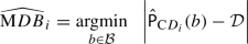  (35)

The closeness of (35) to the MDB of $\mathcal {H}_{i}$ depends on the number of samples N and how $\mathcal {B}$ is formed. These can be determined by the requirements of the application at hand.

4 Identification test and its performance

The identification test, applied following the rejection of $\mathcal {H}_{0}$, can be defined in different ways, e.g. using likelihood-ratio-based test statistics (Teunissen 2006) or information criteria (Akaike 1974; Schwarz 1978). Here, we use one from the former category where the test statistic (Teunissen 2006)

$$\begin{aligned} \underline{T}_{i}=\underline{t}^{T}Q_{tt}^{-1}{C_{t_{i}}}\left( {C_{t_{i}}^{T}}Q_{tt}^{-1}{C_{t_{i}}}\right) ^{-1}{C_{t_{i}}^{T}}Q_{tt}^{-1}\underline{t} \end{aligned}$$

(36)

is formed for all the alternative hypotheses $\mathcal {H}_{i}$ ($i=1,\ldots ,k$). The above test statistic can also be formulated in the least-squares residual vectors of the $\mathcal {H}_{0}$-model, denoted by $\underline{\hat{e}}_{0}$, and the $\mathcal {H}_{i}$-model, denoted by $\underline{\hat{e}}_{i}$, as

$$\begin{aligned} \underline{T}_{{i}}=\Vert \underline{\hat{e}}_{0}\Vert ^{2}_{Q_{yy}}-\Vert \underline{\hat{e}}_{i}\Vert ^{2}_{Q_{yy}} \end{aligned}$$

(37)

Assuming that all the alternative hypotheses are of the same dimension, i.e. $q_{1}=\ldots =q_{k}=q$, (37) suggests that selecting the one with the largest realization of $\underline{T}_{i}$ ($i=1,\ldots ,k$), results in selecting the best-fitting model among all the considered alternatives (Teunissen 2017). This is however not the case when the alternative hypotheses have varying dimensions. As $\underline{T}_{{i}}\overset{\mathcal {H}_{0}}{\sim }\chi ^{2}(q_{i},0)$ and thus $\textsf{E}(\underline{T}_{{i}}|\mathcal {H}_{0})=q_{i}$, the realizations of the test statistic $\underline{T}_{{i}}$ tend to get larger for larger $q_{i}$.

To take the different dimensions of alternative hypotheses into account, we transform all $\underline{T}_{i}$’s so that they have the same distribution under $\mathcal {H}_{0}$, and then compare the transformed test statistics (Teunissen 2017). The Chi-square test statistic $\underline{T}_{{i}}$ can be transformed to a test-statistic with the uniform distribution on the interval [0,  1] (Robert et al. 1999) under $\mathcal {H}_{0}$ as follows

$$\begin{aligned} \underline{\mathcal {S}}_{i}=\textrm{CDF}_{\chi ^{2}(q_{i},0)}\left( \underline{T}_{{i}}\right) \end{aligned}$$

(38)

which is the probability under $\mathcal {H}_{0}$ of obtaining an outcome of the test statistic $\underline{T}_{{i}}$ equal to or less extreme than what was actually observed. Note, $\underline{\mathcal {S}}_{i}$ is one minus the p-value of the test statistic $\underline{T}_{{i}}$ (Lehmann and Lösler 2016). Therefore, if $\mathcal {H}_{0}$ is rejected in the detection step, i.e. $\underline{t}\notin \mathcal {P}_{0}$, the identification test selects $\mathcal {H}_{i}$ if $\underline{t}$ lies in

$$\begin{aligned} \mathcal {P}_{i}=\left\{ t\in \mathbb {R}^{r}\setminus \mathcal {P}_{0}~\Bigg |~\mathcal {S}_{i}=\underset{j\in \{1,\ldots ,k\}}{\max }\;\mathcal {S}_j\right\} ,~i=1,\ldots ,k \end{aligned}$$

(39)

with $\mathcal {S}_{i}$ the realization of $\underline{\mathcal {S}}_{i}$ corresponding with the realization t of $\underline{t}$. In case $q_{1}=\ldots =q_{k}=q$, as $\underline{\mathcal {S}}_{i}$ is an increasing function of $\underline{T}_{i}$, $\mathcal {P}_{i}$ would remain invariant if $\mathcal {S}_{i}$ is replaced with $T_{i}$ in (39).

To understand how using (39) penalizes the acceptance of models with larger number of parameters, i.e. larger $q_{i}$’s, one can for example consider Fisher’s approximation of $\textrm{CDF}_{\chi ^{2}(q_{i},0)}\left( {T}_{{i}}\right)$ which is given by (Fisher 1928; Brown 1974)

$$\begin{aligned} \textrm{CDF}_{\chi ^{2}(q_{i},0)}\left( {T}_{{i}}\right) \approx \textrm{CDF}_{\mathcal {N}(0,1)}\left( \sqrt{2{T}_{{i}}}-\sqrt{2q_{i}-1}\right) \end{aligned}$$

(40)

As a CDF is an increasing function of its argument, (40) implies that $\mathcal {S}_{i}$ is larger for models with a better fit to data (larger ${T}_{i}$), but adds a penalty term for models with larger number of parameters (larger $q_{i}$). Therefore, selecting the alternative hypothesis corresponding with the largest $\mathcal {S}_{i}$ indicates a balance between model fit and the number of parameters.

Fig. 2

An overview of the DIA method when the undecided region is empty. The right panel shows an example partitioning of the misclosure space $\mathbb {R}^{2}$ with three alternative hypotheses, i.e. $k=3$. The coloured scatter plot shows samples of $\underline{t}$ under $\mathcal {H}_{1}$ for some $b_{1}$. The samples leading to the same testing decision are given the same colour

It is easy to verify that the regions (27) and (39) cover the whole misclosure space. Any $t\in \mathbb {R}^{r}{\setminus }\mathcal {P}_{0}$ produces a vector of k realizations $\mathcal {S}_{i}$ ($i=1,\ldots ,k$) combining (36) and (38). For any such t there is a region $\mathcal {P}_i$ in which it lies for some $i\in \{1,\ldots ,k\}$, thus $\bigcup _{i=0}^{k}\,\mathcal {P}_{i}=\mathbb {R}^{r}$. This also implies that the undecided region is empty, i.e. $\mathcal {P}_{k+1}=\emptyset$. The undecided region would however enter if, for instance, the maximum test statistic (38) would further undergo a significance evaluation upon which if turned out not to be significant enough, then the undecided decision is made. In order for the regions (27) and (39) to form a partitioning of the misclosure space, they further need to be mutually disjoint, i.e. $\mathcal {P}_{i}\cap \mathcal {P}_{j}=\emptyset$ for any $i\ne j$. As $\mathcal {P}_{i\ne 0}$’s are defined in $\mathbb {R}^{r}\setminus \mathcal {P}_{0}$, they are all disjoint from $\mathcal {P}_{0}$. For the mutual disjointness of $\mathcal {P}_{i\ne 0}$’s, we have the following result.

Lemma 1

Consider the regions in (39). For any $i\ne j$,

(i) when $q_{i}\ne q_{j}$, then $\mathcal {P}_{i}\cap \mathcal {P}_{j}=\emptyset$ always holds true;

(ii) when $q_{i}=q_{j}$, then $\mathcal {P}_{i}\cap \mathcal {P}_{j}=\emptyset$ if and only if

$$\begin{aligned} C_{t_{i}}^{\perp ^T}C_{t_{j}}\ne 0 \end{aligned}$$

(41)

with $C_{t_{i}}^{\perp }$ a basis matrix of the null space of $C_{t_{i}}^{T}$.

Proof

See ‘Appendix’. $\square$

An overview of the DIA-method with the regions (27) and (39) defining the testing procedure is given in Fig. 2.

4.1 Minimal identifiable bias (MIB)

As the last equality in (10) shows, a high CD-probability ${\mathsf P}_{\textrm{CD}_{i}}(b_i)$ does not necessarily imply a high CI-probability ${\mathsf P}_{\textrm{CI}_{i}}(b_i)$ unless we have the special case of only a single alternative hypothesis with no undecided decision being made. Therefore, in case of multiple hypotheses, the MDB does not provide information about correct identification. To assess the sensitivity of the identification step, one can analyse the MIBs of the alternative hypotheses. The MIB of the alternative hypothesis $\mathcal {H}_{i}$ is defined as the smallest size of $b_{i}$ that can be identified given a certain CI-probability (Teunissen 2018). Note, to evaluate the performance of the identification test, that use has also been made of minimal separable bias (MSB) proposed by (Förstner 1983). The MSB of an alternative hypothesis $\mathcal {H}_{i}$ with respect to the alternative $\mathcal {H}_{j}$ is the smallest size of $b_{i}$ that leads to the wrong identification of $\mathcal {H}_{j}$ given a certain value of $\textrm{WI}_{i,j}$ (Yang et al. 2013, 2021).

The MIB for a given CI-probability $\mathcal {I}$ depends on the probability mass of the PDF of $\underline{t}$ under $\mathcal {H}_{i}$ over $\mathcal {P}_{i}$ (see Table 1). This probability mass is driven by the shape and size of $\mathcal {P}_{i}$, magnitude of $\textsf{E}\left( \underline{t}|\mathcal {H}_{i}\right)$ and its orientation with respect to the borders of $\mathcal {P}_{i}$. Note, if $b_{i}\in \mathbb {R}^{q_{i}>1}$ is a vector, then, a given CI-probability yields different MIBs along different directions in $\mathbb {R}^{q_{i}}$. In this case, a pre-set CI-probability defines a region in $\mathbb {R}^{q_{i}}$ the boundary of which defines the MIBs in different directions. The MIB of $\mathcal {H}_{i}$ for a given CI-probability $\mathcal {I}$ is denoted by $|b_{i,\textrm{MIB}}|$ if $b_{i}\in \mathbb {R}$, and $\Vert b_{i,\textrm{MIB}}(d)\Vert$ along the unit direction $d\in \mathbb {S}^{q_{i}-1}$ if $b_{i}\in \mathbb {R}^{q_{i}>1}$. Therefore, we have

$$\begin{aligned}{} & {} b_{i}\in \mathbb {R}:~\textsf{P}_{\textrm{CI}_{i}}(|b_{i,\mathrm MIB}|)=\mathcal {I} \end{aligned}$$

(42)

$$\begin{aligned}{} & {} b_{i}\in \mathbb {R}^{q_{i}>1}:~\textsf{P}_{\textrm{CI}_{i}}(\Vert b_{i,\mathrm MIB}(d)\Vert d)=\mathcal {I};~d\in \mathbb {S}^{q_{i}-1} \end{aligned}$$

(43)

4.2 Computation of the MIBs

The MIB corresponding with $\mathcal {H}_{i}$ can be found from inverting the bottom equality in Table 1 with $\mathcal {P}=\mathcal {P}_{i}$. This inversion is, however, not trivial as ${\mathsf P}_{\textrm{CI}_{i}}(b_i)$ is an r-fold integral over the complex region $\mathcal {P}_i$. One can take resort to the numerical evaluation technique explained in Sect. 3.2. Using (19), with $\mathcal {F}(\underline{t})=\underline{t}$ and ${\Omega }_{t}={\Omega }=\mathcal {P}_{i}$, the CI-probability ${\mathsf P}_{\textrm{CI}_{i}}(b_{i})$ can be written as

$$\begin{aligned} \begin{array}{lllll} {\mathsf P}_{\textrm{CI}_{i}}(b_{i})= & {} \textsf{E}\left( p_{i}(\underline{t})|\mathcal {H}_{i}\right) \end{array} \end{aligned}$$

(44)

We now use the above equality, to find an approximation of the MIB corresponding with $\mathcal {H}_{i}$ for a given CI-probability of $\mathcal {I}$.

• Generate N independent samples $t^{(1)},\ldots ,t^{(N)}$ from the distribution $f_{\underline{t}}(\tau |\mathcal {H}_{0})$ as discussed in Sect. 2.3.

• For a range of bias magnitudes $b\in \mathcal {B}\subset \mathbb {R}^+$, shift $t^{(s)}$ ($s=1,\ldots ,N$) to

  $$\begin{aligned} \begin{array}{lll} \tilde{t}_{i}^{(s)}(b)=t^{(s)}+C_{t_{i}}b &{}\quad \textrm{if}~b_{i}\in \mathbb {R}\\ \tilde{t}_{i}^{(s)}(b)=t^{(s)}+C_{t_{i}}d\,b &{}\quad \textrm{if}~b_{i}\in \mathbb {R}^{q_{i}>1} \end{array} \end{aligned}$$

  (45)

  to get the samples from the distribution $f_{\underline{t}}(\tau |\mathcal {H}_{i})$.

• For each b, compute an approximation of the CI-probability as

  $$\begin{aligned} \hat{{\mathsf P}}_{\textrm{CI}_{i}}(b) = \frac{\sum _{s=1}^{N} p_{i}\left( \tilde{t}_{i}^{(s)}(b)\right) }{N} \end{aligned}$$

  (46)

• An approximation of the MIB of $\mathcal {H}_{i}$ is given by

  

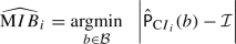  (47)

Similar to the MDB computation, whether (47) provides a close enough approximation to the MIB of $\mathcal {H}_{i}$ is dependent on the number of samples N and how $\mathcal {B}$ is formed.

5 MDBs, MIBs and their propagation into the DIA-estimator

As for a given bias $b_{i}$, the CD-probability exceeds the CI-probability, i.e. ${\mathsf P}_{\textrm{CD}_{i}}(b_{i})\ge {\mathsf P}_{\textrm{CI}_{i}}(b_{i})$, then for equal CD- and CI-probability, we have

$$\begin{aligned} \begin{array}{lll} b_{i}\in \mathbb {R}&{}:&{}|b_{i,\textrm{MIB}}|\ge |b_{i,\textrm{MDB}}| \\ b_{i}\in \mathbb {R}^{q_{i}>1}&{}:&{}\Vert b_{i,\textrm{MIB}}(d)\Vert \ge \Vert b_{i,\textrm{MDB}}(d)\Vert ~\mathrm{for~any~}d\in \mathbb {S}^{q_{i}-1} \end{array} \end{aligned}$$

(48)

In this section, by means of a number of examples, we analyse the MDBs and the MIBs, illustrate their differences and evaluate their impact on the DIA-estimator.

We note that the vector of misclosures $\underline{t}$ is not uniquely defined. This, however, does not affect the outcome of the detection test in Sect. 3 and the identification test in Sect. 4 as both the detector $\Vert \underline{t}\Vert ^2_{Q_{tt}}$ and the test statistic $\underline{\mathcal {S}}_{i}$ remain invariant for any linear one-to-one transformation of the misclosure vector. Therefore, instead of $\underline{t}$, one can for instance also work with

$$\begin{aligned} \bar{\underline{t}}\;=\;\mathcal {G}^{-T}\underline{t}\left\{ \begin{array}{lll} \overset{\mathcal {H}_{0}}{\sim }\mathcal {N}(0,~I_{r}) \\ \overset{\mathcal {H}_{i}}{\sim }\mathcal {N}(\mathcal {G}^{-T}C_{t_{i}}b_{i},~I_{r}) \end{array} \right. \end{aligned}$$

(49)

with the Cholesky-factor $\mathcal {G}^{T}$ of the Cholesky-factorization $Q_{tt}=\mathcal {G}^{T}\mathcal {G}$. The advantage of using $\bar{\underline{t}}$ over $\underline{t}$ lies in the ease of visualizing certain effects due to the identity-variance matrix of $\bar{\underline{t}}$ (Zaminpardaz and Teunissen 2019).

In the following, instead of $\underline{t}$, we work with $\underline{\bar{t}}$. The partitioning corresponding with $\underline{\bar{t}}$ is characterized through

$$\begin{aligned} \begin{array}{lll} \overline{\mathcal {P}}_{0}&{}=&{}\left\{ \bar{t}\in \mathbb {R}^{r}\Bigg |~\Vert \bar{t}\Vert ^{2}\le \chi ^{2}_{1-\textsf{P}_\textrm{FA}}(r,0)\right\} \\ \overline{\mathcal {P}}_{i}&{}=&{}\left\{ \bar{t}\in \mathbb {R}^{r}\setminus \overline{\mathcal {P}}_{0}\Bigg |~\overline{\mathcal {S}}_{i}=\underset{j\in \{1,\ldots ,k\}}{\max } \overline{\mathcal {S}}_{j}\right\} \end{array} \end{aligned}$$

(50)

where

$$\begin{aligned} \overline{\mathcal {S}}_{i}=\textrm{CDF}_{\chi ^{2}(0,{q_{i}})}(\overline{T}_{i});~\overline{T}_{i}=\left\| \bar{C}_{t_{i}}^{T}\bar{t}\right\| ^{2}_{\bar{C}_{t_{i}}^{T}\bar{C}_{t_{i}}};~\bar{C}_{t_{i}}=\mathcal {G}^{-T}C_{t_{i}} \end{aligned}$$

(51)

Therefore, $\overline{\mathcal {P}}_{0}$ contains $\bar{t}$’s inside and on a zero-centred sphere with the radius of $\sqrt{\chi ^{2}_{1-\textsf{P}_\textrm{FA}}(r,0)}$. Note, in our examples, we work with alternative hypotheses of the same dimension, i.e. $q_{1}=\ldots =q_{k}=q$. Therefore, the regions $\overline{\mathcal {P}}_{i\ne 0}$ in (50) can equivalently be formed by replacing $\overline{\mathcal {S}}_{i}$ with $\overline{T}_{i}$.

Fig. 3

A levelling network, consisting of two loops, running through three points with two of them being benchmarks (black triangles). In each levelling loop, there are two instrument set-ups between one of the benchmarks and the unknown point. The blue curves indicate the observed height differences. The arrow on each blue curve indicates the direction of the observed height difference

5.1 Levelling network: detection only

To determine the height of a point, denoted by $x\in \mathbb {R}$, two levelling loops are designed between the point and two different benchmarks, i.e. BM$_{1}$ and BM$_2$, as shown in Fig. 3. In each levelling loop, we assume two instrument set-ups. Let $\underline{\Delta h}_{i}\in \mathbb {R}^{2}$ ($i=1,2$) contain the height difference measurements collected between BM$_{i}$ and the unknown point. We then define $\underline{y}=[\underline{h}_{1}^{T},~\underline{h}_{2}^{T}]^{T}\in \mathbb {R}^{4}$ with $\underline{h}_{i}=\underline{\Delta h}_{i}+[h_{\textrm{BM}_{i}},-h_{\textrm{BM}_{i}}]^{T}$ and $h_{\textrm{BM}_{i}}$ the known height of BM$_{i}$. Under the null hypothesis $\mathcal {H}_{0}$, the observations are assumed to be bias-free, whereas under the alternative hypotheses $\mathcal {H}_{i}$ ($i=1,2$), it is assumed that the observation pair $\underline{\Delta h}_{i}$, and thus $\underline{h}_{i}$, are biased by $b_{i}\in \mathbb {R}^{2}$ ($i=1,2$). Assuming that the observations are uncorrelated and equally precise with the same standard deviation $\sigma$, the null and alternative hypotheses are formulated as:

$$\begin{aligned} \begin{array}{lllll} \mathcal {H}_{0}&{}:&{}\textsf{E}(\underline{y})=\left( e_{2}\otimes e_{2}^{\perp }\right) \,x,&{}\textsf{D}(\underline{y})=\sigma ^{2}I_{4} \\ \mathcal {H}_{i}&{}:&{}\textsf{E}(\underline{y})=\underbrace{\left( e_{2}\otimes e_{2}^{\perp }\right) }_{A}\,x+\underbrace{\left( u_{i}^{2}\otimes I_{2}\right) }_{C_{i}}b_{i},&{}\textsf{D}(\underline{y})=\sigma ^{2}I_{4} \end{array} \end{aligned}$$

(52)

where $\otimes$ shows the Kronecker product (Henderson et al. 1983), $e_{*}\in \mathbb {R}^{*}$ the vector of ones, $e_{2}^{\perp }=[1,~-1]^T$ is orthogonal to $e_{2}$, $I_{*}\in \mathbb {R}^{*\times *}$ the identity matrix, and $u^{2}_{i}\in \mathbb {R}^{2}$ the canonical unit vector having one as its $i\text {th}$ element and zeros otherwise. Under $\mathcal {H}_{0}$, there are $r=4-1=3$ redundancies; the two levelling loops contribute a redundancy of 2, while the third redundancy comes from having a second benchmark available.

Let us assume that testing is restricted to detection only where one aims to check the validity of $\mathcal {H}_{0}$. In this case, $\overline{\mathcal {P}}_1 = \mathbb {R}^{r}{\setminus }\overline{\mathcal {P}}_0$ becomes the undecided region for which no parameter solution is provided. The DIA-estimator of x is then given by (11) setting $k=0$ and $F^{T}=1$, i.e.

$$\begin{aligned} \tilde{\underline{x}}=\left\{ \begin{array}{ll}\underline{\hat{x}}_{0} &{}~~\textrm{if} ~~\bar{\underline{t}}\in \overline{\mathcal {P}}_{0} \\ \textrm{unavailable} &{} ~~\textrm{if} ~~\bar{\underline{t}}\notin \overline{\mathcal {P}}_{0}\end{array}\right. \end{aligned}$$

(53)

Evaluation of the DIA-estimator would only be possible if $\mathcal {H}_{0}$ gets accepted, i.e. $\underline{\bar{t}}\in \overline{\mathcal {P}}_{0}$, upon which one needs to consider

$$\begin{aligned} \bar{\underline{x}}=\tilde{\underline{x}}|\bar{\underline{t}}\in \overline{\mathcal {P}}_{0}=\underline{\hat{x}}_{0} \end{aligned}$$

(54)

where use has been made of the independence of $\underline{\hat{x}}_{0}$ and $\bar{\underline{t}}$ (cf. 5).

The MDB under each alternative hypothesis $\mathcal {H}_{i}$ ($i=1,2$) shows the minimal size of $\mathcal {H}_{i}$-bias that leads to rejection of $\mathcal {H}_{0}$ with a probability $\mathcal {D}$, thus declaring $\tilde{\underline{x}}$ unavailable. For both $\mathcal {H}_{1}$ and $\mathcal {H}_{2}$ in (52), $b_{i}$ ($i=1,2$) is a 2-vector, i.e. $b_{i}=[b_{i,1},~b_{i,2}]^{T}$, and thus their MDBs can be computed using (31) as

$$\begin{aligned} \Vert b_{i,\textrm{MDB}}(d)\Vert =\dfrac{2\sigma \lambda ({\mathsf P}_\textrm{FA}, \mathcal {D},r)}{\sqrt{2+(d^{T}e_{2})^{2}}};\;d\in \mathbb {S};~i=1,2 \end{aligned}$$

(55)

If the unit vector d sweeps the boundary of the unit circle, an ellipse is obtained which defines the MDBs in different directions. Figure 4 [top] shows the MDB-to-noise ratio ellipse, i.e. $\Vert b_{i,\textrm{MDB}}(d)\Vert /\sigma$, assuming ${\mathsf P}_\textrm{FA}=0.1$ and $\mathcal {D}=0.8$. The smallest MDB is obtained when d is parallel to $e_{2}$, while the largest MDB is obtained when d is parallel to $e_{2}^{\perp }$. This can be understood by the contribution of $\mathcal {H}_{i}$-biases to the misclosure vector. An $\mathcal {H}_{i}$-bias parallel to $e_{2}^{\perp }$ means that the height-difference measurements in Loop i are biased by the same amount but in opposite directions. The biases in the two height-difference measurements will then cancel out each other when adding up the measurements to form the the misclosure of the corresponding levelling loop, hence not being sensed by that misclosure. On the other hand, an $\mathcal {H}_{i}$-bias parallel to $e_{2}$ means that both of the height-difference measurements in Loop i are biased by the same amount and in the same direction. These biases will propagate into the misclosure of the corresponding levelling loop, affecting it by twice the individual observation biases.

Fig. 4

[Top] MDB-to-noise ratio ellipse for testing the validity of $\mathcal {H}_{0}$ in (52) using (27), given ${\mathsf P}_\textrm{FA}=0.1$ and $\mathcal {D}=0.8$. [Bottom] The influential BNR (56) as a function of the top MDB-to-noise ratio ellipse

In case the $\mathcal {H}_{i}$-bias goes unnoticed and $\mathcal {H}_{0}$ is incorrectly accepted, the DIA-estimator generated by (54), i.e. $\underline{\hat{x}}_{0}$, would be biased. The influence of the undetected $\mathcal {H}_{i}$-MDB along the direction $d\in \mathbb {S}$ on $\underline{\hat{x}}_{0}$ can be described by the influential bias-to-noise ratio (BNR)

$$\begin{aligned} \begin{array}{lll} \lambda _{\hat{x}_{0,i}}(d)&{}=&{}\dfrac{|\textsf{E}(\underline{\hat{x}}_{0}-x|\mathcal {H}_{i})|}{\sigma _{\hat{x}_{0}}}\\ &{}=&{}\dfrac{\left| d^{T}e_{2}^{\perp }\right| }{2}\cdot \dfrac{\Vert b_{i,\textrm{MDB}}(d)\Vert }{\sigma }\\ &{}=&{} \dfrac{\left| d^{T}e_{2}^{\perp }\right| }{\sqrt{2+(d^{T}e_{2})^{2}}}\cdot \lambda ({\mathsf P}_\textrm{FA}, \mathcal {D},r) \end{array} \end{aligned}$$

(56)

which is a measure of the external reliability (Baarda 1968; Teunissen 2006). The larger the influential BNR $\lambda _{\hat{x}_{0,i}}(d)$, the more significant an $\mathcal {H}_{i}$-bias of MDB-size is for estimation of the unknown height. The above influential BNR is shown in Fig. 4 [bottom] as a function of the MDB-to-noise ratio ellipse in Fig. 4 [top]. The influential bias, for a given set of $\{{\mathsf P}_\textrm{FA}, \mathcal {D},r\}$, is zero when d is parallel to $e_{2}$, while reaches its maximum when d is parallel to $e_{2}^{\perp }$. Each of the four height-difference measurements in (52) yields a solution for x. As all these measurements are equally precise, the BLUE of x is nothing else but the average of the each of the four individual solutions. When the height-difference measurements in Loop i are biased by the same amount and in the same directions (d parallel to $e_{2}$), the biases in the two height-difference measurements will then cancel out each other when averaging out the individual solutions, hence not influencing the BLUE of x.

5.2 Levelling network: detection+identification

Fig. 5

Partitioning of the misclosure space $\mathbb {R}^{3}$ corresponding with $\underline{\bar{t}}$ (49) using (50). The grey sphere shows the boundary of $\overline{\mathcal {P}}_{0}$ with ${\mathsf P}_\textrm{FA}=0.1$, while the orthogonal blue and purple planes separate $\overline{\mathcal {P}}_{1}$ from $\overline{\mathcal {P}}_{2}$

Fig. 6

MDB- and MIB-to-noise ratio curves for testing the hypotheses in (52) using (50), given ${\mathsf P}_\textrm{FA}=0.1$. The panels from left to right correspond to equal CD- and CI probabilities $\mathcal {D}=\mathcal {I}=$ 0.4, 0.6, 0.8 and 0.99, respectively

We now consider, for the levelling network in (52), a testing procedure consisting of both detection and identification steps using (50). It can easily be verified that $\bar{C}_{t_{1}}^{\perp ^T}\bar{C}_{t_{2}}\ne 0$, which according to Lemma 1 means that the regions $\overline{\mathcal {P}}_{0}$, $\overline{\mathcal {P}}_{1}$ and $\overline{\mathcal {P}}_{2}$ cover the whole misclosure space $\mathbb {R}^{3}$, implying that the undecided region is empty. Figure 5 shows the partitioning of the misclosure space $\mathbb {R}^{3}$ induced by these regions. The grey sphere shows the boundary of $\overline{\mathcal {P}}_{0}$ choosing ${\mathsf P}_\textrm{FA}=0.1$. The regions $\overline{\mathcal {P}}_{1}$ and $\overline{\mathcal {P}}_{2}$ are separated from each other by the following two planes:

$$\begin{aligned} \bar{\tau }^{T}\left( \dfrac{\bar{C}_{t_{1}}^{\perp }}{\Vert \bar{C}_{t_{1}}^{\perp }\Vert }\pm \dfrac{\bar{C}_{t_{2}}^{\perp }}{\Vert \bar{C}_{t_{2}}^{\perp }\Vert }\right) =0;~\bar{\tau }\in \mathbb {R}^{3} \end{aligned}$$

(57)

As the above planes are the locus of the points with both $\overline{\mathcal {S}}_{1}$ and $\overline{\mathcal {S}}_{2}$ (cf. 51) being the maximum of $\{\overline{\mathcal {S}}_{1},\overline{\mathcal {S}}_{2}\}$, the plane equations are obtained by equating $\overline{\mathcal {S}}_{1}$ and $\overline{\mathcal {S}}_{2}$. The two planes are orthogonal to each other implying that $\overline{\mathcal {P}}_{1}$ and $\overline{\mathcal {P}}_{2}$ are the same in shape and size. This indeed makes sense as $\mathcal {H}_{1}$-biases and $\mathcal {H}_{2}$-biases make the same contributions to the misclosure vector. Therefore, in addition to their MDBs, their MIBs are also the same along any $d\in \mathbb {S}$.

MDB versus MIB. The MDB- and MIB-to-noise ratio curves for $\mathcal {H}_{i}$ ($i=1,2$) are illustrated in Fig. 6 for different values of $\mathcal {D}=\mathcal {I}$, assuming ${\mathsf P}_\textrm{FA}=0.1$. In each panel, in agreement with (48), the MIB curve, in blue, encompasses the MDB curve, in black. The MDB and the MIB are very close to each other along the direction of $e_{2}$, i.e. when the height-difference measurements in Loop i are biased by the same amount and in the same direction, which can be explained as follows. A bias vector $b_{i}$ parallel to $e_{2}$ makes $\textsf{E}(\bar{\underline{t}}|\mathcal {H}_{i})$ bisect the normals of the orthogonal planes in (57). In this case, $\textsf{E}(\bar{\underline{t}}|\mathcal {H}_{i})$ lies at its farthest position from the two planar borders of $\overline{\mathcal {P}}_{1}$ and $\overline{\mathcal {P}}_{2}$, meaning that most of the probability mass of the PDF of $\bar{\underline{t}}$ that lies outside $\overline{\mathcal {P}}_{0}$ falls into the region $\overline{\mathcal {P}}_{i}$, see Fig. 7. As a result, ${\mathsf P}_{\textrm{CD}_{i}}(b_{i})$ and ${\mathsf P}_{\textrm{CI}_{i}}(b_{i})$ are very close to each other for a given bias along $e_{2}$, or alternatively the MDB and the MIB are very close to each other along $e_{2}$ for a pre-set $\mathcal {D}=\mathcal {I}$. The difference between the MDB and the MIB increases when the bias direction deviates from $e_{2}$ towards $e_{2}^{\perp }$.

The $\mathcal {H}_{1}$-bias and $\mathcal {H}_{2}$-bias of the same size affect the misclosure vector in the exact same way if $b_{1}$ and $b_{2}$ are parallel to $e_{2}^{\perp }$, i.e. when the height-difference measurements in Loop $i=1,2$ are biased by the same amount but in opposite directions. In this case, none of the loop misclosures would sense the bias, and the third misclosure, formed by having a second benchmark, senses the same magnitude of the individual measurement bias. Therefore, upon the rejection of $\mathcal {H}_{0}$, the probability of identifying $\mathcal {H}_{1}$ is the same as that of $\mathcal {H}_{2}$, i.e. $\textsf{P}_{\textrm{CI}_{i}}(b_{i})=0.5\textsf{P}_{\textrm{CD}_{i}}(b_{i})$, if $b_{i}$ is parallel to $e_{2}^{\perp }$ ($i=1,2$). This indicates that the CI-probability of $\mathcal {H}_{i}$ cannot reach above 0.5, which explains the bands around the direction of $e_{2}^{\perp }$ in Fig. 6 when $\mathcal {I}\ge 0.5$.

Propagation of the MDB–MIB into the DIA-estimator. With the testing procedure in (50), the DIA-estimator of the unknown height is given by

$$\begin{aligned} \underline{\bar{x}}\;=\;\underline{\hat{x}}_{0}\,\bar{p}_{0}(\underline{\bar{t}})\;+\;\underline{\hat{x}}_{1}\,\bar{p}_{1}(\underline{\bar{t}})\;+\;\underline{\hat{x}}_{2}\,\bar{p}_{2}(\underline{\bar{t}}) \end{aligned}$$

(58)

with $\bar{p}_{i}({\bar{t}})$ being the indicator function of region $\overline{\mathcal {P}}_{i}$. As was stated in the previous subsection, $\underline{\hat{x}}_{0}$ is the average of the four solutions obtained from the individual height-difference measurements. The estimators $\underline{\hat{x}}_{i\ne 0}$ are obtained by excluding the pair of measurements in Loop i.

Figure 8 [top] shows $\lambda _{\bar{x}_{i}}$ (cf. 17) as a function of MIB-to-noise ratio for a given CI-probability of $\mathcal {I}=0.8$. It is observed that $\lambda _{\bar{x}_{i}}=0$, i.e. $\underline{\bar{x}}$ is unbiased, when the height-difference measurements in Loop i are biased by the same amount and in the same directions ($b_{i}$ parallel to $e_{2}$). This can be explained as follows. Let $b_{i}=\gamma e_{2}$ for some $\gamma \in \mathbb {R}$. It can be easily verified that $A^{+}C_{i}{b}_{{i}}=0$, and, as $\bar{C}_{t_{i}}b_{i}$ bisects the normals of the planar borders in Fig. 5, that the probability mass of the PDF $f_{\bar{\underline{t}}}(\bar{\tau }|\mathcal {H}_{i})$ in all the regions $\overline{\mathcal {P}}_{0}$, $\overline{\mathcal {P}}_{1}$ and $\overline{\mathcal {P}}_{2}$ is symmetric with respect to $\bar{C}_{t_{i}}b_{i}$. In this case, $\textsf{E}(\underline{\bar{t}}\bar{p}_{j}(\underline{\bar{t}})|\mathcal {H}_{i})$ will be parallel to $\bar{C}_{t_{i}}b_{i}$, i.e. $\textsf{E}(\underline{\bar{t}}\bar{p}_{j}(\underline{t})|\mathcal {H}_{i})=\beta \, \bar{C}_{t_{i}}b_{i}$ for some $\beta \in \mathbb {R}$, and thus $\bar{C}_{t_{j}}^{+}\textsf{E}(\underline{\bar{t}}\bar{p}_{j}(\underline{t})|\mathcal {H}_{i})=-0.5\beta (e_{2}^{\perp }e_{2}^{\perp ^T})b_{i}=0$. Therefore, if $b_{i}$ is parallel to $e_{2}$, then $A^{+}\bar{b}_{y_{i}}=0$, implying that $\underline{\bar{x}}$ is unbiased under $\mathcal {H}_{i}$. The DIA-estimator becomes biased when $b_{i}$ is not parallel to $e_{2}$, with the amount of bias increasing when the direction of $b_{i}$ changes from $e_{2}$ towards $e_{2}^{\perp }$.

Fig. 7

Probability mass of the PDF of $\bar{\underline{t}}$ under $\mathcal {H}_{1}$ (black sphere) over the partitioning regions for a bias of $b_{1}=2\sigma \,e_{2}$

Fig. 8

[Top] MDB- (in black) and MIB-to-noise ratio (in blue) curves for testing the hypotheses in (52) using (50), given ${\mathsf P}_\textrm{FA}=0.1$ and $\mathcal {D}=\mathcal {I}=0.8$. The red curve shows $\lambda _{\bar{x}_{i}}$ (cf. 17) for (58) as a function of the MIB-to-noise ratio curve. [Bottom] The graphs of $\lambda _{\bar{x}_{i}}$ for the detection-only and detection+identification case as a function of the orientation of the top MDBs and the MIBs, respectively

The bottom panel in Fig. 8 compares the propagation of the MDBs and the MIBs to the detection-only and detection+identification DIA-estimators as a function of the bias orientation for $\mathcal {D}=\mathcal {I}=0.8$, respectively. With identification being included in the testing procedure, the bias-effect in the DIA-estimator can become much larger depending on the bias orientation. However, one should note, with detection only, that there will be ‘unavailability’, which is not the case when both detection and identification are applied. In fact, if the detection-only and detection+identification cases have the same settings for the false-alarm, i.e. the same $\mathcal {P}_{0}$, then under a particular alternative hypothesis, the times that $\mathcal {H}_{0}$ is correctly rejected (i.e. times of unavailability with the detection-only case under this alternative hypothesis) are the times that identification is done for the detection+identification case.

5.3 GNSS single-point positioning

Let a GNSS receiver track single-frequency pseudorange (code) measurements of $m=\sum _{i=1}^{s}m_{i}$ satellites belonging to s constellations. The corresponding linearized single-point positioning (SPP) model based on these code observations will then include $n=3+s$ unknowns including three receiver coordinate increments and s receiver clock errors. Let $\underline{y}=\left[ \underline{y}^{T}_{1}\ldots \underline{y}^{T}_{s}\right] ^{T}\in \mathbb {R}^{m}$ with $\underline{y}_{i}\in \mathbb {R}^{m_i}$ containing the code observables from the $i\text {th}$ constellation. Assuming that all the code observations are uncorrelated and of the same precision $\sigma$, $\underline{y}$ can be modelled under $\mathcal {H}_{0}$ as

$$\begin{aligned} \mathcal {H}_{0}:~\textsf{E}(\underline{y})=\left[ \begin{array}{cccc}G_{1}&{} e_{m_{1}}&{}&{}\\ \vdots &{}&{}\ddots \\ G_{s}&{}&{}&{} e_{m_{s}} \end{array}\right] \,x,\quad \textsf{D}(\underline{y})= \sigma ^{2}\,I_{m} \end{aligned}$$

(59)

where $G_{i}\in \mathbb {R}^{m_{i}\times 3}$ contains the satellite-to-receiver unit direction vectors as its rows, and $x\in \mathbb {R}^{3+s}$ the receiver North-East-Up coordinate increments and the receiver clock errors for the s constellations.

As alternative hypotheses, we will restrict our attention to those describing outliers in individual observations and assume that only one observation at a time is affected by an outlier. In that case there are as many alternative hypotheses as there are observations, i.e. $k=m$. The observational model under $\mathcal {H}_{i}$ ($i=1,\ldots ,m$) is then given by

$$\begin{aligned}{} & {} \mathcal {H}_{i}:~\textsf{E}(\underline{y})=\left[ \begin{array}{cccc}G_{1}&{} e_{m_{1}}&{}&{}\\ \vdots &{}&{}\ddots \\ G_{s}&{}&{}&{} e_{m_{s}} \end{array}\right] \,x\;+\;c_{i}\,b_{i},\quad \nonumber \\{} & {} \textsf{D}(\underline{y})= \sigma ^{2}\,I_{m} \end{aligned}$$

(60)

with $c_{i}\in \mathbb {R}^{m}$ the canonical unit vector having one as its $i\text {th}$ element and zeros otherwise, and $b_{i}\in \mathbb {R}$ the unknown outlier. Our testing procedure to test the hypotheses in (59) and (60) involves both detection and identification steps as specified by the partitioning regions (50). Note, since the alternatives in (60) are one-dimensional, that $\overline{\mathcal {P}}_{i\ne 0}$ can equivalently be formulated in Baarda’s w-test statistic (Baarda 1967; Teunissen 2006) as

$$\begin{aligned} \overline{\mathcal {P}}_{i}=\left\{ \bar{t}\in \mathbb {R}^{r}\setminus \overline{\mathcal {P}}_{0}\Bigg |~|w_{i}|=\underset{j\in \{1,\ldots ,k\}}{\max } |w_{j}|\right\} \end{aligned}$$

(61)

where

$$\begin{aligned} w_{i}={\bar{c}_{{i}}^{T}\bar{t}},~ \bar{c}_{i}=\dfrac{1}{\Vert \bar{c}_{t_{i}}\Vert }\bar{c}_{t_{i}},~\bar{c}_{t_i}=\mathcal {G}^{-T}c_{t_{i}},~c_{t_{i}}=B^{T}c_{i} \end{aligned}$$

(62)

with $\bar{c}_{i}$ a unit vector showing the direction of $\textsf{E}(\bar{\underline{t}}|\mathcal {H}_{i})=b_{i}\Vert \bar{c}_{t_{i}}\Vert \bar{c}_{i}$. $\overline{\mathcal {P}}_{i\ne 0}$ includes all $\bar{t}$’s outside the sphere $\overline{\mathcal {P}}_{0}$ which, among $\bar{c}_{j}$’s for $j=1,\ldots , m$, make the smallest angle with $\bar{c}_{i}$. The border between two adjacent regions $\overline{\mathcal {P}}_{i\ne 0}$ and $\overline{\mathcal {P}}_{j\ne 0}$ is then the bisector of the angle formed by the corresponding unit vectors $\bar{c}_{i}$ and $\bar{c}_{j}$. The cosine of this angle gives the correlation coefficient between $\underline{w}_{i}$ and $\underline{w}_{j}$ (Förstner 1983). The larger the correlation coefficient, the closer the two vectors $\bar{c}_{i}$ and $\bar{c}_{j}$ would be to the border between $\overline{\mathcal {P}}_{i\ne 0}$ and $\overline{\mathcal {P}}_{j\ne 0}$.

Fig. 9

[Left] Skyplot view of the receiver-satellite geometry. The six blue circles denote the skyplot position of the satellites. [Right] Partitioning of the misclosure space $\mathbb {R}^{2}$ formed by $\overline{\mathcal {P}}_{0}$ and $\overline{\mathcal {P}}_{i}$, for $i=1,\ldots ,6$, (cf. 50), for the hypotheses in (59) and (60), assuming ${\mathsf P}_\textrm{FA}=0.1$ and $\sigma =30$cm

Example 1

The skyplot in Fig. 9 [left] shows the geometry of GPS satellites as viewed from Melbourne at an epoch on 13 November 2021, with a cut-off elevation of $10^{\circ }$. The satellites have been labelled with their PRN as well as the index of the alternative hypothesis capturing the outlier in their code observation. With six GPS satellites, two misclosures can be formed under $\mathcal {H}_{0}$ in (59), i.e. $r=2$. Figure 9 [right] shows the partitioning of the misclosure space $\mathbb {R}^{2}$ corresponding with $\underline{\bar{t}}$ (cf. 49), assuming ${\mathsf P}_\textrm{FA}=0.1$ and $\sigma =30$cm. In addition to the partitioning regions $\overline{\mathcal {P}}_{0}$ and $\overline{\mathcal {P}}_{i}$ ($i=1,\ldots ,6$), the unit vectors $\bar{c}_{i}$ in (62) are also illustrated.

In Fig. 10 [top], the solid and the dashed curves, respectively, show the MDB- and the MIB-to-noise ratio as a function of the pre-set CD- and CI-probabilities. The graphs associated with different alternative hypotheses are distinguished using different colours. The signature of the MDB of an alternative hypothesis is generally different from its MIB. This is due to the fact that the MDB of $\mathcal {H}_{i}$ for a given CD-probability is driven only by $\Vert \bar{c}_{t_{i}}\Vert$ (cf. 30), while its MIB is in addition driven by $\overline{\mathcal {P}}_{i}$ and the orientation of $\bar{c}_{i}$, i.e. the orientation of $\textsf{E}(\bar{\underline{t}}|\mathcal {H}_{i})$, w.r.t. the straight borders of $\overline{\mathcal {P}}_{i}$. The larger the norm $\Vert \bar{c}_{t_{i}}\Vert$ is, the smaller both the MDB and the MIB. Also, the MIB gets smaller if the region $\overline{\mathcal {P}}_{i}$ gets wider and/or the vector $\bar{c}_{i}$ gets closer to the bisector line of the angle between the two straight borders of $\overline{\mathcal {P}}_{i}$, see (Zaminpardaz and Teunissen (2019), Lemma 2). The latter happens when there are small correlations among the w-test statistics. The difference between the factors contributing to the MDB and the MIB can be well-understood by the following two examples:

• $\mathcal {H}_{1}$ versus $\mathcal {H}_{4}$: The MDB graphs of these hypotheses are close to each other which is due to the proximity of $\Vert \bar{c}_{t_{4}}\Vert \approx 0.35/\sigma$ to $\Vert \bar{c}_{t_{1}}\Vert \approx 0.37/\sigma$. However, $\overline{\mathcal {P}}_{1}$ is wider compared to $\overline{\mathcal {P}}_{4}$. Also $\bar{c}_{1}$ lies almost halfway between the straight borders of $\overline{\mathcal {P}}_{1}$, while $\bar{c}_{4}$ is close to one of the straight borders of $\overline{\mathcal {P}}_{4}$. These make the MIB graphs of $\mathcal {H}_{4}$ and $\mathcal {H}_{1}$ dramatically differ from each other.

• $\mathcal {H}_{1}$ versus $\mathcal {H}_{2}$: Despite the MDB of $\mathcal {H}_{1}$ being larger than that of $\mathcal {H}_{2}$, the MIB of $\mathcal {H}_{1}$ is smaller than that of $\mathcal {H}_{2}$. The former results from $\Vert \bar{c}_{t_{1}}\Vert \approx 0.37/\sigma$ being smaller than $\Vert \bar{c}_{t_{2}}\Vert \approx 0.49/\sigma$. Looking at the right panel of Fig. 9, we note that $\overline{\mathcal {P}}_{2}$ has smaller area compared to $\overline{\mathcal {P}}_{1}$. In addition, while $\bar{c}_{1}$ lies almost halfway between the straight borders of $\overline{\mathcal {P}}_{1}$, $\bar{c}_{2}$ is close to one of the straight borders of $\overline{\mathcal {P}}_{2}$. These make the MIB graph of $\mathcal {H}_{1}$ being lower than that of $\mathcal {H}_{2}$.

Figure 10 [middle] shows the graphs of the difference between the MDB- and the MIB-to-noise ratio, as a function of the pre-set probability for different alternative hypotheses. Depending on the alternative hypothesis and the pre-set probability, the MIB can be significantly larger than the MDB. For example, under $\mathcal {H}_{4}$, the MIB-MDB difference at $\mathcal {D}=\mathcal {I}=0.95$ is as big as $|b_{4,\textrm{MIB}}|-|b_{4,\textrm{MDB}}|\approx 48\sigma$. Therefore, using MDB to infer the identifiability of alternative hypotheses could provide a misleading description of the testing performance.

Figure 10 [bottom] illustrates the impact of the MDB- and the MIB-sized biases, under different alternative hypotheses, on the detection-only and detection+identification DIA-estimators of the receiver coordinates $\vartheta =[I_{3},~0]x$, by showing the scalar $\lambda _{\bar{\vartheta }_{i}}$ (cf. 17) as a function of the corresponding probability. We note that the dashed curves in this figure show almost the same signature; they first increase and then decrease to zero. The CI-probability approaches one when the probability mass of $f_{\bar{\underline{t}}}(\bar{\tau }|\mathcal {H}_{i})$ in the regions $\overline{\mathcal {P}}_{j\ne i}$ approaches zero. In this case, we have $\textsf{E}(\bar{\underline{t}}\bar{p}_{j}(\bar{\underline{t}})|\mathcal {H}_{i})\rightarrow 0$ and $\textsf{E}(\bar{\underline{t}}\bar{p}_{i}(\bar{\underline{t}})|\mathcal {H}_{i})\rightarrow \bar{c}_{t_{i}}b_{i}$, resulting in $\bar{b}_{y_{i}}\rightarrow 0$ (cf. 16), which explains the close-to-zero value of $\lambda _{\bar{\vartheta }_{i}}$ when $\mathcal {I}$ is close to one. At a given CI-probability $\mathcal {I}$, among the six alternative hypotheses, $\lambda _{\bar{\vartheta }_{i}}$ reaches largest values under $\mathcal {H}_{2}$ and $\mathcal {H}_{4}$. This is also consistent with the MIB graphs of these hypotheses in Fig. 10 [top] which lie on top of those of the other alternatives. The solid curves in Fig. 10 [bottom] show an increasing behaviour as a function of CD-probability. This is due to the fact that the amount of bias in $\underline{\hat{\vartheta }}_{0}$ is an increasing function of the MDB and the MDB is an increasing function of the pre-set CD-probability. $\square$

Fig. 10

[Top] Graphs of the MDB-to-noise ratio (solid lines) and the MIB-to-noise (dashed lines) of different alternative hypotheses as a function of pre-set CD- and CI-probabilities. The results correspond to the hypotheses in (59) and (60), and the misclosure space partitioning in Fig. 9. [Middle] The difference between the solid curves and the dashed curves of the same colour in the top panel. [Bottom] The graphs of $\lambda _{\bar{\vartheta }_{i}}$ as a function of the CD-probability (solid lines) and the CI-probability (dashed lines) for the detection-only and detetion+identification case, respectively

Fig. 11

Partitioning of the misclosure space $\mathbb {R}^{2}$ formed by $\overline{\mathcal {P}}_{0}$ and $\overline{\mathcal {P}}_{i}$, for $i=1,2,3$, (cf. 50), for the hypotheses in (59) and (60), assuming ${\mathsf P}_\textrm{FA}=0.1$ and $\sigma =30$cm

Fig. 12

[Top] Graphs of the MDB-to-noise ratio (solid lines) and the MIB-to-noise (dashed lines) of different alternative hypotheses as a function of pre-set CD- and CI-probabilities. The results correspond to the hypotheses in (59) and (60) for $k=3$, and the misclosure space partitioning in Fig. 11. [Middle] The difference between the solid curves and the dashed curves of the same colour in the top panel. [Bottom] The graphs of $\lambda _{\bar{\vartheta }_{i}}$ as a function of the CD-probability (solid lines) and the CI-probability (dashed lines) for the detection-only and detection+identification case, respectively

Example 2

The purpose of this example is to illustrate that one always should be diligent when including alternative hypotheses in the testing process. In this example, we show what happens to the testing performance and the quality of the DIA-estimator when the set of alternative hypotheses increases. Let us assume that outliers in the code observations of three high-elevation satellites in Example 1, i.e. G12, G6 and G2, do not occur. In that case, instead of six alternative hypotheses, there would be $k=3$ modelling code outliers of the other three satellites. The partitioning of the misclosure space is then formed by four regions as shown in Fig. 11. With fewer alternative hypotheses, the regions corresponding with $\mathcal {H}_{2}$ and $\mathcal {H}_{3}$ get larger compared to their counterparts in Fig. 9, thus leading to higher correct identification probabilities for these hypotheses. Figure 12 presents the same type of information as Fig. 10 but for the testing procedure illustrated in Fig. 11. Comparing the panels of Fig. 12 with those in Fig. 10, we note a reduction in the MIB-to-noise ratio of $\mathcal {H}_{2}$ and $\mathcal {H}_{3}$. As a result, the detection+identification DIA-estimator gets less biased for MIB-sized biases in the observations under $\mathcal {H}_{2}$ and $\mathcal {H}_{3}$. $\square$

Fig. 13

[Top] Skyplot view of the satellite geometries. The blue circles denote the skyplot position of the satellites. [Middle] The difference between the MDB-to-noise ratio and the MIB-to-noise (dashed lines) of different alternative hypotheses as a function of pre-set CD- and CI-probabilities. The results correspond to the hypotheses in (59) and (60), assuming $\sigma =30$cm and ${\mathsf P}_\textrm{FA}=0.1$. [Bottom] The graphs of $\lambda _{\bar{\vartheta }_{i}}$ as a function of the CD-probability (solid lines) and the CI-probability (dashed lines) for the detection-only and detetion+identification case, respectively

Example 3

Figure 13 [top] shows the geometry of GPS and Galileo satellites as viewed from Melbourne at an epoch on 13 November 2021, with a cut-off elevation of $10^\circ$. The satellites have been labelled with their PRN as well as the index of the alternative hypothesis capturing the outlier in their code observation. The redundancy of the SPP model under $\mathcal {H}_{0}$ for this dual-system geometry is $r=20-3-2=15$. The middle panel shows the difference between the MDB- and the MIB-to-noise ratio, as a function of the pre-set probability for different alternative hypotheses. Despite Example 1, this MDB–MIB difference is not very significant. Furthermore, as the bottom panel shows, the amount of measurement error that gets propagated into the DIA-estimator of the receiver coordinates is much less than the previous example. $\square$

6 Summary and concluding remarks

In this contribution, we studied the multi-hypotheses performance of the detection and identification steps in the DIA method, and the impact they have on the produced DIA-estimator. It was emphasized that while the detection capability is assessed using the well-known concept of the minimal detectable bias (MDB), use should be made of the minimal identifiable bias (MIB) when it comes to the testing identification performance.

The testing and estimation elements of the DIA method were discussed using a canonical model formulation of the null hypothesis and a partitioning of misclosure space. Through this partitioning, we discriminated between different statistical events including correct detection (CD) and correct identification (CI). The probability of the occurrence of the former indicates the sensitivity of the detection step whereas that of the latter indicates the sensitivity of the identification step. By inverting the CD- and CI-probability integrals, the testing sensitivity analysis can be done by means of the MDBs and MIBs in observation space.

In the detection step, we used the overall model test. For the identification test, we formulated a test statistic taking into account varying dimensions of the alternative hypotheses. We presented the numerical algorithms for computing the corresponding MDBs and MIBs, and also their propagation into the nonlinear DIA-estimator. These algorithms were then applied to a number of examples so as to illustrate and analyse the difference between detection-only and detection+identification.

The first example was a simple levelling network for which we applied two testing schemes: (1) detection-only and (2) detection+identification. It was shown that depending on the alternative hypothesis and the bias direction, the MDB and the MIB could be significantly different from each other. Thus, using MDB to infer the identifiability of alternative hypotheses could provide a misleading description of the testing performance. It was further demonstrated that with the detection+identification testing procedure, the bias-effect in the DIA-estimator can become much larger compared to the detection-only case. However, one should note, with detection only, that there will be ‘unavailability’, which is not the case when both detection and identification are applied.

Our analysis was further continued for GNSS single-point positioning examples when outlier detection+identification is applied. It was demonstrated that the signature of a pseudorange-MDB is generally different from a pseudorange-MIB. For example, while two different alternatives have very close MDB values, their MIBs can significantly differ from each other. It was thereby also highlighted that reducing the number of alternative hypotheses would lead to smaller MIBs. This emphasizes that due diligence is needed when including alternative hypotheses in the testing process. Finally, in this study, our numerical examples were given considering alternative hypotheses of the same dimension. An MDB–MIB analysis as a function of the dimension of alternative hypothesis is the topic of future works.

Appendix

Proof of Lemma 1

(i) Let us assume that $\mathcal {P}_{i}\cap \mathcal {P}_{j}\ne \emptyset$ for $i\ne j$. Then, for some $t\in \mathbb {R}^{r}/\mathcal {P}_{0}$, we have

$$\begin{aligned} \textrm{CDF}_{\chi ^{2}(0,q_{i})}\left( \Vert P_{C_{t_{i}}}t\Vert ^{2}_{Q_{tt}}\right) =\textrm{CDF}_{\chi ^{2}(0,q_{j})}\left( \Vert P_{C_{t_{j}}}t\Vert ^{2}_{Q_{tt}}\right) \end{aligned}$$

(63)

with $P_{C_{t_{i}}}=C_{t_{i}}(C_{t_{i}}^{T}Q_{tt}^{-1}C_{t_{i}})^{-1}C_{t_{i}}^{T}Q_{tt}^{-1}$ being the orthogonal projector that projects onto the range space of $C_{t_i}$. We now show that the probability of $\underline{t}$ satisfying (63) is zero. Let us define the continuous random vectors/variables

$$\begin{aligned} \begin{array}{lll} \underline{t}_{i}=P_{C_{t_{i}}}\underline{t},~&{}\underline{z}_{i}=\textrm{CDF}_{\chi ^{2}(0,q_{i})}\left( \Vert \underline{t}_{i}\Vert ^{2}_{Q_{tt}}\right) \\ \underline{t}_{j}=P_{C_{t_{j}}}\underline{t},~&{}\underline{z}_{j}=\textrm{CDF}_{\chi ^{2}(0,q_{j})}\left( \Vert \underline{t}_{j}\Vert ^{2}_{Q_{tt}}\right) \end{array} \end{aligned}$$

(64)

Since $q_{i}\ne q_{j}$, then $\textrm{CDF}_{\chi ^{2}(0,q_{i})}(\cdot )$ and $\textrm{CDF}_{\chi ^{2}(0,q_{j})}(\cdot )$ are the same only if their input is zero. Therefore, $\underline{z}_{i}=\underline{z}_{j}$ when $\underline{t}_{i}=\underline{t}_{j}=0$. As $P_{C_{t_{i}}}\ne P_{C_{t_{j}}}$, then $\underline{t}_{ij}=\underline{t}_{i}-\underline{t}_{j}$ is a continuous random vector, and thus we have $\textsf{P}(\underline{t}_{ij}=0)=0$, implying that $\textsf{P}(\underline{z}_{i}=\underline{z}_{j})=0$. Therefor, the probability of $\underline{t}$ satisfying (63) is zero, meaning that $\mathcal {P}_{i}\cap \mathcal {P}_{j}=\emptyset$ for any $i\ne j$ with $q_{i}\ne q_{j}$.

(ii) ‘if’ part: Let us assume that $\mathcal {P}_{i}\cap \mathcal {P}_{j}\ne \emptyset$ for $i\ne j$. Then, as $q_{i}=q_{j}$, for some $t\in \mathbb {R}^{r}/\mathcal {P}_{0}$, we have

$$\begin{aligned} \Vert P_{C_{t_{i}}}t\Vert ^{2}_{Q_{tt}}=\Vert P_{C_{t_{j}}}t\Vert ^{2}_{Q_{tt}} \end{aligned}$$

(65)

from which two conclusions can be made: 1) $(P_{C_{t_{i}}}-P_{C_{t_{j}}})t=0$; 2) $P_{C_{t_{i}}}=P_{C_{t_{j}}}$. With $\underline{t}_{ij}=(P_{C_{t_{i}}}-P_{C_{t_{j}}})\underline{t}$ being a continuous random vector, we have $\textsf{P}(\underline{t}_{ij}=0)=0$, meaning that the probability of the occurrence of the former conclusion is zero. Also, the latter conclusion contradicts our earlier assumption of $C_{t_{i}}^{\perp ^T}C_{t_{j}}\ne 0$. Therefore, $\mathcal {P}_{i}\cap \mathcal {P}_{j}=\emptyset$ for any $i\ne j$ with $q_{i}=q_{j}$.

‘only if’ part: Let us assume that $C_{t_{i}}^{\perp ^T}C_{t_{j}}=0$, i.e. $P_{C_{t_{i}}}=P_{C_{t_{j}}}$, for $i\ne j$. Then, given (36) and (38), we have $\mathcal {S}_{i}=\mathcal {S}_{j}$ for any $t\in \mathbb {R}^{r}$. This reveals that $\mathcal {P}_{i}=\mathcal {P}_{j}$ which contradicts our earlier assumption of $\mathcal {P}_{i}\cap \mathcal {P}_{j}=\emptyset$. Therefore, $C_{t_{i}}^{\perp ^T}C_{t_{j}}\ne 0$ for any $i\ne j$ with $q_{i}=q_{j}$. $\square$

References

Akaike H (1974) A new look at the statistical model identification. IEEE Trans Autom Control 19(6):716–723
Arnold SF (1981) The theory of linear models and multivariate analysis. Wiley, New York
Baarda W (1967) Statistical concepts in geodesy. Netherlands Geodetic Commission, Oude
Baarda W (1968) A testing procedure for use in geodetic networks. Netherlands Geodetic Commission, Oude
Brown JR (1974) Error analysis of some normal approximations to the chi-square distribution. J Acad Mark Sci 2(3):447–454
Costa AFB, Magalhães MSD, Epprecht EK (2010) Th e non-central chi-square chart with double sampling. Braz J Oper Prod Manage 2:21–38
Durdag UM, Hekimoglu S, Erdogan B (2018) Reliability of models in kinematic deformation analysis. J Surv Eng 144(3):04018004
Fisher RA (1928) Statistical methods for research workers, 2nd edn. Oliver and Boyd, Edinburgh
Förstner W (1983) Reliability and discernability of extended Gauss-Markov models. In: Deut. Geodact. Komm. Seminar on math models of geodetic photogrammetric point determination with regard to outliers and systematic errors, p 79-104(SEE N 84-26069 16-43)
Gillissen I, Elema IA (1996) Test results of DIA: a real-time adaptive integrity monitoring procedure, used in an integrated naviation system. Int Hydrogr Rev 73(1):75–100
Haynam G, Govindarajulu Z, Leone F, Siefert P (1982) Tables of the cumulative non-central chi-square distribution-part l. Stat J Theoret Appl Stat 13(3):413–443
Henderson HV, Pukelsheim F, Searle RS (1983) On the history of the Kronecker product. Linear Multilinear Algebra 14:113–120
Hewitson S, Wang J (2006) GNSS receiver autonomous integrity monitoring (RAIM) performance analysis. GPS Solut 10(3):155–170
Imparato D, Teunissen PJG, Tiberius CCJM (2019) Minimal detectable and identifiable biases for quality control. Surv Rev 51(367):289–299
Jonkman NF, De Jong K (2000) Integrity monitoring of Igex-98 data, part ii: cycle slip and outlier detection. GPS Solut 3(4):24–34
Khodabandeh A, Teunissen PJG (2016) Single-epoch GNSS array integrity: an analytical study. In: Sneeuw N, Novák P, Crespi M, Sansò F (eds) VIII Hotine–Marussi symposium on mathematical geodesy: proceedings of the symposium in Rome. Springer International Publishing, New York
Kuusniemi H, Lachapelle G, Takala JH (2004) Position and velocity reliability testing in degraded GPS signal environments. GPS Solut 8(4):226–237
Lehmann R, Lösler M (2016) Multiple outlier detection: hypothesis tests versus model selection by information criteria. J Surv Eng 142(4):04016017
Lehmann R, Lösler M (2017) Congruence analysis of geodetic networks-hypothesis tests versus model selection by information criteria. J Appl Geodesy 11(4):271–283
Lehmann R, Voß-Böhme A (2017) On the statistical power of Baarda’s outlier test and some alternative. J Geodetic Sci 7(1):68–78
Nowel K (2020) Specification of deformation congruence models using combinatorial iterative Dia testing procedure. J Geodesy 94(12):1–23
Robert CP, Casella G, Casella G (1999) Monte Carlo statistical methods. Springer, New York
Schwarz G (1978) Estimating the dimension of a model. The Ann Stat 56:461–464
Teunissen PJG (1985) Quality control in geodetic networks. In: Grafarend E, Sanso F (eds) Optimization and design of geodetic networks. Springer, Berlin
Teunissen P (1990) Quality control in integrated navigation systems. IEEE Aerosp Electron Syst Mag 5(7):35–41
Teunissen PJG (2006) Testing theory: an introduction, 2nd edn. Delft University Press, Delft
Teunissen PJG (2017) Batch and recursive model validation. In: Teunissen PJG, Montenbruck O (eds) Springer Handbook of global navigation satellite systems. Springer, Cham
Teunissen PJG (2018) Distributional theory for the DIA method. J Geodesy 92(1):59–80. https://doi.org/10.1007/s00190-017-1045-7
Tienstra J (1956) Theory of the adjustment of normally distributed observation. Argus, Amsterdam
Verhoef HME, De Heus HM (1995) On the estimation of polynomial breakpoints in the subsidence of the Groningen Gasfield. Surv Rev 33(255):17–30
Yang L, Wang J, Knight NL, Shen Y (2013) Outlier separability analysis with a multiple alternative hypotheses test. J Geodesy 87:591–604
Yang L, Li Y, Wu Y, Rizos C (2014) An enhanced MEMS-INS/GNSS integrated system with fault detection and exclusion capability for land vehicle navigation in urban areas. GPS Solut 18(4):593–603
Yang L, Shen Y, Li B, Rizos C (2021) Simplified algebraic estimation for the quality control of dia estimator. J Geodesy 95:1–15
Yavaşoğlu HH, Kalkan Y, Tiryakioğlu I, Yigit CO, Özbey V, Alkan MN, Bilgi S, Alkan RM (2018) Monitoring the deformation and strain analysis on the Ataturk Dam, Turkey. Geomat Nat Haz Risk 9(1):94–107
Zaminpardaz S (2016) Horizon-to-elevation mask: A potential benefit to ionospheric gradient monitoring. In: Proceedings of the 29th international technical meeting of the satellite division of the institute of navigation (ION GNSS+ 2016), pp 1764–1779
Zaminpardaz S, Teunissen PJG (2019) DIA-datasnooping and identifiability. J Geodesy 93(1):85–101
Zaminpardaz S, Teunissen P, Nadarajah N, Khodabandeh A (2015) GNSS array-based ionospheric spatial gradient monitoring: precision and integrity analyses. In: Proceedings of the ION 2015 Pacific PNT Meeting, pp 799–814
Funding
Open Access funding enabled and organized by CAUL and its Member Institutions.
Author information
Authors and Affiliations
Corresponding author