
Abstract
This paper examines the monetary transmission mechanism in the Euro area (EA) for the period of single monetary policy using factor-augmented vector autoregressive (FAVAR) techniques. The aims of the paper are threefold. First, a novel dataset consisting of 120 disaggregated macroeconomic time series spanning the period 1999:M1 through 2011:M12 is gathered for the EA as an aggregate. Second, a Bayesian joint estimation technique of the FAVAR approach is applied to the European data in order to investigate the impacts of monetary policy shocks on the economy. Third, time variation in the transmission mechanism and the impact of the global financial crisis are investigated in the FAVAR context using a rolling windows technique. We find that there are considerable gains from the implementation of the Bayesian technique such as smoother impulse response functions and statistical significance of the estimates. According to our rolling estimations, consumer prices and monetary aggregates display the most time-variant responses to the monetary policy shocks in the EA.


Notes
The summaries of the techniques employed in our study are described in Sect. 2.
See Sect. 4.2.1 for details of determining the pre-crisis period.
See Sect. 2.2 for details.
For further details, see BBE (2005), pp. 400–401.
See Depoutot et al. (1998) for details of the software.
When either the first or the last observation of a series is missing, Demetra+ does not provide any estimation. For this kind of occasional observations, using a MATLAB code obtained from Bańbura and Modugno (2010), we replaced the missing values by the median of the series and then applied a centred MA(3) to the replaced observations. We thank the authors for kindly sharing the replication files of their paper.
We thank Fabio Canova for suggesting this scaling during the presentation of the paper at 2011 Royal Economic Society Easter School held at the University of Birmingham.
We thank Schumacher and Breitung (2008) for making the replication files of their paper publicly available, and also thank Christian Schumacher for sharing the files and his comments with us. Our tests are based on the replication files of the paper.
For software details, see Lütkepohl and Krätzig (2004).
Capacity utilisation rate, gross domestic product, final consumption expenditure, gross fixed capital formation.
Total employment, total employees, total self-employed, real labour productivity per person employed, real unit labour cost.
Earnings per employee, wages and salaries.
Current, capital and financial accounts.
A similar approach has been used by Soares (2011) for the EA in order to have a panel of monthly macroeconomic time series consisting of the variables we have interpolated for our own dataset.
See Sect. 4.2 for details.
The estimation results are found to be robust to the number of Gibbs iterations.
Fig. 1 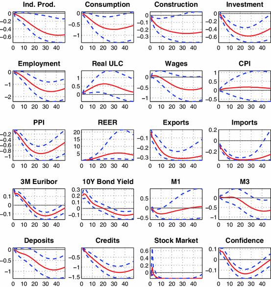
Baseline results. Note Consumption final consumption expenditure, Construction construction production index, Investment gross fixed capital formation, Euribor the Euro interbank offered rate, Deposits total deposits of residents held at monetary financial institutions (MFI), Credits credits to total residents granted by MFI, Confidence consumer confidence indicator
Unsurprisingly, short-term interest rates follow the responses of the policy variable, which, if we recall, is the only observable factor in the transition Equation (2), and its impulse responses can also be calculated in standard ways.
The failure of the negative correlations between nominal interest rates and the money stock expected to be created by monetary policy disturbances. See Kelly et al. (2011).
i.e. \(\hat{\varLambda }^f \hat{F}_t + \hat{\varLambda }^y Y_t\) in the observation Eq. 1.
See Boivin et al. (2008, p. 2).
We thank Gary Koop for valuable discussions and comments during the presentation of the paper at the \(6\mathrm{th}\) annual Bayesian econometrics workshop organised by the Rimini Centre for Economic Analysis (RCEA) in Rimini, Italy in 2011.
Additionally, despite many and quite long trials with the replication files of Koop and Korobilis (2009) to fit both one- and two-step TVP-FAVAR models to our relatively short dataset, we could not obtain any reasonable results. We anyway thank the authors for making the files available to the public.
Still with four factors and two lags.
Only 6-month rolling is estimated by the one-step method. For details, see below.
First three observations are lost due to data transformations explained above in Sect. 3.1.
See Appendix 2.1.
Estimating our FAVAR model window by window means identification of a new 25 basis-point shock specific to that particular sample.
i.e. the monetary authority of the EA which consists of the ECB and national central banks of the countries in the monetary union.
Remember, first 2,000 iterations are discarded in order to eliminate the influence of our choice of starting values.

References
Ahmadi P (2005) Measuring the effects of a shock to monetary policy: a factor-augmented vector autoregression (FAVAR) approach with agnostic identification. PhD thesis, Humboldt University
Ahmadi P, Uhlig H (2007) Measuring the dynamic effects of monetary policy shocks: a Bayesian FAVAR approach with sign restrictions. Manuscript, University of Chicago
Altissimo F, Benigno P, Palenzuela DR (2011) Inflation differentials in a currency area: facts, explanations and policy. Open Econ Rev 22(2):189–233
Altissimo F, Bassanetti A, Cristadoro R, Forni M, Hallin M, Lippi M, Reichlin L, Veronese G (2001) EuroCOIN: a real time coincident indicator of the euro area business cycle. CEPR Working Paper No 3108
Bai J, Ng S (2002) Determining the number of factors in approximate factor models. Econometrica 70(1):191–221
Bai J, Ng S (2007) Determining the number of primitive shocks in factor models. J Bus Econ Stat 25(1): 52–60
Bańbura M, Giannone D, Reichlin L (2008) Large Bayesian VARs. ECB Working Paper No 966
Bańbura M, Modugno M (2010) Maximum likelihood estimation of factor models on data sets with arbitrary pattern of missing data. ECB Working Paper No 1189
Barnett A, Mumtaz H, Theodoridis K (2012) Forecasting UK GDP growth, inflation and interest rates under structural change: a comparison of models with time-varying parameters. Bank of England Working Paper No 450
Belviso F, Milani F (2006) Structural factor-augmented VAR (SFAVAR) and the effects of monetary policy. Top Macroecon 6(3):1443–1443
Bernanke B, Blinder A (1992) The federal funds rate and the channels of monetary transmission. Am Econ Rev 82(4):901–921
Bernanke B, Boivin J, Eliasz P (2005) Measuring the effects of monetary policy: a factor-augmented vector autoregressive (FAVAR) approach. Q J Econ 120(1):387–422
Bernanke B, Boivin J, Eliasz P (2004) Measuring the effects of monetary policy: a factor-augmented vector autoregressive (FAVAR) approach. NBER Working Paper No 10220
Blaes B (2009) Money and monetary policy transmission in the euro area: evidence from FAVAR and VAR approaches. Deutsche Bundesbank Discussion Paper, Series 1: Economic Studies (18)
Boivin J, Giannoni M, Mojon B (2008) How has the euro changed the monetary transmission? In: Acemoglu RKD, Woodford M (eds) NBER Macroeconomics Annual 2008, chap 2, vol 23. University of Chicago Press, Chicago, pp 77–125
Boivin J, Giannoni M, Mihov I (2009) Sticky prices and monetary policy: evidence from disaggregated US data. Am Econ Rev 99(1):350–384
Boivin J, Giannoni M (2007) Global forces and monetary policy effectiveness. NBER Working Paper No 13736
Bork L (2009) Estimating US monetary policy shocks using a factor-augmented vector autoregression: an EM algorithm approach. CREATES Research Papers 2009–2011, School of Economics and Management, University of Aarhus
Braun P, Mittnik S (1993) Misspecifications in vector autoregressions and their effects on impulse responses and variance decompositions. J Econ 59(3):319–341
Canova F, Ferroni F, de France B (2012) The dynamics of US inflation: can monetary policy explain the changes? J Econ 167:47–60
Carter C, Kohn R (1994) On Gibbs sampling for state space models. Biometrika 81(3):541–553
Chow G, Lin A (1971) Best linear unbiased interpolation, distribution, and extrapolation of time series by related series. Rev Econ Stat 53(4):372–375
Connor G, Korajczyk R (1993) A test for the number of factors in an approximate factor model. J Finance 48:1263–1291
Cragg J, Donald S (1997) Inferring the rank of a matrix. J Econ 76(1):223–250
Cushman D, Zha T (1997) Identifying monetary policy in a small open economy under flexible exchange rates. J Monet Econ 39(3):433–448
Depoutot R, Dossé J, Hoffmann S, Planas C (1998) Advanced seasonal adjustment interface DEMETRA. Eurostat, Luxembourg
Donald S (1997) Inference concerning the number of factors in a multivariate nonparametric relationship. Econometrica 65:103–131
ECB (2010) Monetary policy transmission in the euro area, a decade after the introduction of the Euro. Mon Bull:85–98
Eickmeier S, Breitung J (2006) How synchronized are new EU member states with the euro area? Evidence from a structural factor model. J Comp Econ 34(3):538–563
Eickmeier S (2009) Comovements and heterogeneity in the euro area analyzed in a non-stationary dynamic factor model. J Appl Econ 24(6):933–959
Forni M, Reichlin L (1998) Let’s get real: a factor analytical approach to disaggregated business cycle dynamics. Rev Econ Stud 65(3):453–473
Forni M, Hallin M, Lippi M, Reichlin L (2000) The generalized dynamic-factor model: identification and estimation. Rev Econ Stat 82(4):540–554
Forni M, Lippi M (2001) The generalized dynamic factor model: representation theory. Econ Theory 17(06):1113–1141
Gelman A, Rubin D (1992a) A single sequence from the Gibbs sampler gives a false sense of security. Bayesian Stat 4:625–631
Gelman A, Rubin D (1992b) Inference from iterative simulation using multiple sequences. Stat Sci 7: 457–472
Geman S, Geman D (1984) Stochastic relaxation, Gibbs distributions, and the Bayesian restoration of images. IEEE Trans Pattern Anal Mach Intell 6:721–741
Geweke J (1977) The dynamic factor analysis of economic time series models. Social Systems Research Institute, University of Wisconsin, Madison
Giannone D, Reichlin L, Sala L (2004) Monetary policy in real time. NBER Macroecon Annu 19:161–200
Kapetanios G (2010) A testing procedure for determining the number of factors in approximate factor models with large datasets. J Bus Econ Stat 28(3):397–409
Kelly L, Barnett W, Keating J (2011) Rethinking the liquidity puzzle: application of a new measure of the economic money stock. J Banking Finance 35(4):768–774
Kim C, Nelson C (1999) State-space models with regime switching. MIT Press, Cambridge
Koop G, Korobilis D (2009) Bayesian multivariate time series methods for empirical macroeconomics. Found Trends Econ 3:267–358
Korobilis D (2012) Assessing the transmission of monetary policy using time-varying parameter dynamic factor models. Oxf Bull Econ Stat 75:157–179
Leeper E, Sims C, Zha T, Hall R, Bernanke B (1996) What does monetary policy do? BPEA 2:1–78
Lewbel A (1991) The rank of demand systems: theory and nonparametric estimation. J Econ Soc 59:711–730
Lütkepohl H, Krätzig M (2004) Applied time series econometrics. Cambridge University Press, Cambridge
Lütkepohl H (2005) New introduction to multiple time series analysis. Springer, Berlin
Marcellino M, Stock JH, Watson MW (2000) A dynamic factor analysis of the EMU. Mimeo
McCallum A, Smets F (2007) Real wages and monetary policy transmission in the euro area. Kiel Working Paper 1360, Kiel Institute for the World Economy
McCulloch R, Rossi P (1994) An exact likelihood analysis of the multinomial probit model. J Econ 64(1–2):207–240
Mumtaz H, Surico P (2007) The transmission of international shocks: a factor augmented VAR approach. Mimeo, Bank of England
Mumtaz H, Surico P (2009) The transmission of international shocks: a factor-augmented VAR approach. J Money Credit Banking 41:71–100
Mumtaz H, Zabczyk P, Ellis C (2011) What lies beneath?. A time-varying FAVAR model for the UK transmission mechanism, ECB Working Paper No 1320
Raftery A, Lewis S (1992) How many iterations in the Gibbs sampler. Bayesian Stat 4(2):763–773
Raftery A, Lewis S (1996), Implementing MCMC. Markov chain Monte Carlo, in practice pp 115–130
Sargent T, Sims C (1977) Business cycle modeling without pretending to have too much a priori economic theory. New Methods Bus Cycle Res 1:145–168
Schumacher C, Breitung J (2008) Real-time forecasting of German GDP based on a large factor model with monthly and quarterly data. Int J Forecast 24(3):386–398
Sims C (1972) Money, income, and causality. Am Econ Rev 62(4):540–552
Sims C (1980a) Comparison of interwar and postwar business cycles: monetarism reconsidered. Am Econ Rev 70(2):250–257
Sims C (1980b) Macroeconomics and reality. Econometrica 48(1):1–48
Sims C (1992) Interpreting the macroeconomic time series facts: the effects of monetary policy. Eur Econ Rev 36(5):975–1011
Soares R (2011) Assessing monetary policy in the euro area: a factor-augmented VAR approach. Banco de Portugal Working Papers
Stock J, Watson M (1999) Forecasting inflation. J Monet Econ 44(2):293
Stock J, Watson M (2002a) Forecasting using principal components from a large number of predictors. J Am Stat Assoc 97(460):1167–1179
Stock J, Watson M (2002b) Macroeconomic forecasting using diffusion indexes. J Bus Econ Stat 20: 147–162
Stock J, Watson M (1998) Diffusion indexes. NBER Working Paper No 6702
Stock J, Watson M (2005) Implications of dynamic factor models for VAR analysis. NBER Working Paper No 11467
Uhlig H (2005) What are the effects of monetary policy on output? Results from an agnostic identification procedure. J Monet Econ 52(2):381–419
Zivot E, Wang J (2006) Modeling financial time series with S-PLUS, vol 13. Springer, New York
Acknowledgments
This paper was written while I was a Ph.D. candidate at the University of Birmingham, UK. Therefore, I would like to express my gratefulness to my supervisor Anindya Banerjee for his valuable guidance and great support. I would also like to thank my co-supervisor John Fender, the staff of the Department of Economics and my colleagues for their comments.
Author information
Authors and Affiliations
Corresponding author
Appendices
Appendices
1.1 1: Data description
Details of our dataset are as follows. The transformation (Tr.) codes are 1—no transformation; 2—first difference; 5—first difference of logarithm. The variables denoted as ‘1’ (‘0’) in column 4 are assumed to be slow- (fast-) moving. Data details in brackets apply to the following same category series unless otherwise stated. An asterisk (*) denotes the variable is originally available in quarterly frequency.
No. | Description | Tr. | S/F | Source |
|---|---|---|---|---|
1 | Industrial Production (IP) Total (2005\(=\)100) | 5 | 1 | OECD |
2 | IP-Intermediate Goods | 5 | 1 | Eurostat |
3 | IP-Energy | 5 | 1 | Eurostat |
4 | IP-Capital Goods | 5 | 1 | Eurostat |
5 | IP-Durable Consumer Goods | 5 | 1 | Eurostat |
6 | IP-Non-Durable Consumer Goods | 5 | 1 | Eurostat |
7 | IP-Mining And Quarrying | 5 | 1 | Eurostat |
8 | IP-Manufacturing | 5 | 1 | Eurostat |
9 | IP-New Orders | 5 | 1 | Eurostat |
10 | Construction Production Index | 5 | 1 | Eurostat |
11 | Unemployment Rate (\(\%\)) | 1 | 1 | Eurostat |
12 | Youth Unemployment Rate | 1 | 1 | Eurostat |
13 | Unemployment Total (1000 persons) | 5 | 1 | Eurostat |
14 | Retail Sale Of Food, Beverages And Tobacco\(^a\) | 5 | 1 | Eurostat |
15 | Retail Sale Of Non-Food Products | 5 | 1 | Eurostat |
16 | Retail Sale Of Textiles | 5 | 1 | Eurostat |
17 | Retail Trade | 5 | 1 | Eurostat |
18 | Passenger Car Registration (\(2005=100\)) | 5 | 1 | OECD |
19 | Exports Total (World, Trade value, Mil. Euro) | 5 | 1 | Eurostat |
20 | Imports Total | 5 | 1 | Eurostat |
21 | Total Reserves Including Gold (Mil. Euro) | 5 | 1 | ECB |
22 | HICP All-Items(\(2005=100\)) | 5 | 1 | Eurostat |
23 | Overall Index Exc. Energy and Unp. Food | 5 | 1 | Eurostat |
24 | HICP-Energy And Unprocessed Food | 5 | 1 | Eurostat |
25 | HICP-Liquid Fuels | 5 | 1 | Eurostat |
26 | HICP-Goods | 5 | 1 | Eurostat |
27 | HICP-Services | 5 | 1 | Eurostat |
28 | HICP-Non-Energy Ind. Goods, Durables | 5 | 1 | Eurostat |
29 | HICP-Non-Energy Ind. Goods, Non-Durables | 5 | 1 | Eurostat |
30 | PPI-Industry | 5 | 1 | Eurostat |
31 | PPI-Intermediate and Capital Goods | 5 | 1 | Eurostat |
32 | PPI-Durable Consumer Goods | 5 | 1 | Eurostat |
33 | PPI-Non-Durable Consumer Goods | 5 | 1 | Eurostat |
34 | PPI-Mining and Quarrying | 5 | 1 | Eurostat |
35 | PPI-Manufacturing | 5 | 1 | Eurostat |
36 | Crude Oil (West Texas Intermediate, $/BBL) | 5 | 0 | WSJ |
37 | CRB Spot Index (\(1967=100\)) | 5 | 0 | CRB |
38 | ECB Commodity Price Index (\(2000=100\)) | 5 | 0 | ECB |
39 | 3M Euribor (\(\%\)) | 1 | 0 | Datastream |
40 | 6M Euribor | 1 | 0 | Datastream |
41 | 1Y Euribor | 1 | 0 | Datastream |
42 | 5Y Gov. Bond Yield | 1 | 0 | Datastream |
43 | 10Y Gov. Bond Yield | 1 | 0 | OECD |
44 | Spread 3M-REFI | 1 | 0 | Calculated |
45 | Spread 6M-REFI | 1 | 0 | Calculated |
46 | Spread 1Y-REFI | 1 | 0 | Calculated |
47 | Spread 5Y-REFI | 1 | 0 | Calculated |
48 | Spread 10Y-REFI | 1 | 0 | Calculated |
49 | Euro Stoxx 50 (Points) | 5 | 0 | Eurostat |
50 | Stock Price Index-Basic Materials | 5 | 0 | Datastream |
51 | Stock Price Index-Industrials | 5 | 0 | Datastream |
52 | Stock Price Index-Consumer Goods | 5 | 0 | Datastream |
53 | Stock Price Index-Health Care | 5 | 0 | Datastream |
54 | Stock Price Index-Consumer Services | 5 | 0 | Datastream |
55 | Stock Price Index-Telecommunication | 5 | 0 | Datastream |
56 | Stock Price Index-Financials | 5 | 0 | Datastream |
57 | Stock Price Index-Technology | 5 | 0 | Datastream |
58 | Stock Price Index-Utilities | 5 | 0 | Datastream |
59 | Currency in Circulation (Mil. Euro) | 5 | 0 | Eurostat |
60 | Capital And Reserves | 5 | 0 | Eurostat |
61 | Money Stock: M1 | 5 | 0 | ECB |
62 | Money Stock: M2 | 5 | 0 | ECB |
63 | Money Stock: M3 | 5 | 0 | ECB |
64 | Deposits with Agreed Maturity up to 2Y | 5 | 0 | Eurostat |
65 | External Assets | 5 | 0 | Eurostat |
66 | External Liabilities | 5 | 0 | Eurostat |
67 | Total Deposits of Residents Held At MFI | 5 | 0 | Eurostat |
68 | Overnight Deposits | 5 | 0 | Eurostat |
69 | Repurchase Agreements | 5 | 0 | Eurostat |
70 | Credit to Total Residents Granted by MFI | 5 | 0 | Eurostat |
71 | Loans to General Govt. Granted by MFI | 5 | 0 | Eurostat |
72 | Loans to Other Residents Granted By MFI | 5 | 0 | Eurostat |
73 | Debt Securities of EA Residents | 5 | 0 | Eurostat |
74 | Central Bank Claims on Banking Institutions | 5 | 0 | Eurostat |
75 | Economic Sentiment Indicator(\(\%\)) | 1 | 0 | Eurostat |
76 | Construction Confidence Indicator | 1 | 0 | Eurostat |
77 | Industrial Confidence Indicator | 1 | 0 | Eurostat |
78 | Retail Confidence Indicator | 1 | 0 | Eurostat |
79 | Consumer Confidence Indicator | 1 | 0 | Eurostat |
80 | Services Confidence Indicator | 1 | 0 | Eurostat |
81 | Employment Expec. for the Months Ahead | 1 | 0 | Eurostat |
82 | Production Expec. for the Months Ahead | 1 | 0 | Eurostat |
83 | Selling Price Expec. for the Months Ahead | 1 | 0 | Eurostat |
84 | Assessment of Order Books | 1 | 0 | Eurostat |
85 | Price Trends Over The Next 12 Months | 1 | 0 | Eurostat |
86 | IP-USA(2005=100) | 5 | 1 | OECD |
87 | IP-UK | 5 | 1 | OECD |
88 | IP-JP | 5 | 1 | OECD |
89 | CPI-USA | 5 | 1 | OECD |
90 | CPI-UK | 5 | 1 | OECD |
91 | CPI-JP | 5 | 1 | OECD |
92 | US Federal Funds Target Rate (\(\%\)) | 1 | 0 | FED |
93 | UK Bank Of England Base Rate | 1 | 0 | BoE |
94 | JP Overnight Call Money Rate | 1 | 0 | BoJ |
95 | 10Y Bond Yield USA | 1 | 0 | OECD |
96 | 10Y Bond Yield UK | 1 | 0 | OECD |
97 | 10Y Bond Yield JP | 1 | 0 | OECD |
98 | Stock Price Index-USA (Dow 30, Points) | 5 | 0 | Reuters |
99 | Stock Price Index-UK(FTSE 100, Points) | 5 | 0 | Reuters |
100 | Stock Price Index-JP (Nikkei 225, Points) | 5 | 0 | Reuters |
101 | US Dollar-Euro (Monthly average) | 5 | 0 | Eurostat |
102 | Pound Sterling-Euro | 5 | 0 | Eurostat |
103 | Swiss Franc-Euro | 5 | 0 | Eurostat |
104 | Japanese Yen-Euro | 5 | 0 | Eurostat |
105 | REER (1999 \(=\) 100) | 5 | 0 | Eurostat |
106 | Capacity Utilisation Rate (\(\%\))* | 1 | 1 | ECB |
107 | Gross Domestic Product at Market Prices\(^b\)* | 5 | 1 | Eurostat |
108 | Final Consumption Expenditure* | 5 | 1 | Eurostat |
109 | Gross Fixed Capital Formation* | 5 | 1 | Eurostat |
110 | Employment Total (1000 persons)* | 5 | 1 | Eurostat |
111 | Employees Total* | 5 | 1 | Eurostat |
112 | Self-Employed Total* | 5 | 1 | Eurostat |
113 | Real Labour Productivity/Person Employed\(^c\)* | 5 | 1 | ECB |
114 | Real Unit Labour Cost* | 5 | 1 | Eurostat |
115 | Earnings per Employee (Current, Euro)* | 5 | 1 | Oxford Economics |
116 | Wages and Salaries (Current, Bil. Euro)* | 5 | 1 | Oxford Economics |
117 | Current Account (Net, Mil. Euro, World)* | 2 | 1 | OECD |
118 | Capital Account* | 2 | 1 | OECD |
119 | Financial Account* | 2 | 1 | OECD |
120 | REFI (\(\%\)) | 1 | 0 | Eurostat |
1.2 2: Two-step estimation results
This section contains the estimation results suggested by the two-step FAVAR method.
1.2.1 Baseline and time variation results

Rolling windows—two-step—12M

Rolling windows—two-step—6M. Note In order to be able to present other windows clearly, sample Sep00–Dec08 is eliminated from the figures due to very strange impact of Sep–Dec 2008, we believe, on the impulse responses. Some of the results from this window can be observed in an extended version of Appendix 2, available upon request

Rolling windows—two-step—3M. Note In order to be able to present other windows clearly, sample Sep00–Dec08 is eliminated from the figures due to very strange impact of Sep–Dec 2008, we believe, on the impulse responses. Some of the results from this window can be observed in an extended version of Appendix 2, available upon request
1.3 3: Rolling windows: confidence intervals

Rolling windows—IP

Rolling windows—CPI


Rolling windows—M1

Rolling windows—M3
1.4 4: Alternative model specifications
1.4.1 Number of factors

Alternative model specifications: number of factors. Note The impulse responses are obtained with the two-step method estimated with two lags. Two-step approach is chosen here only because of its computational simplicity

Number of factors: \(R^2\)—all variables

Number of factors: \(R^2\)—main variables
1.4.2 Lag length
See Fig. 15.

Alternative model specifications: lag length. Note The impulse responses are obtained with the two-step method estimated with four factors
1.5 5: Convergence of gibbs samplings
1.5.1 Baseline results
See Fig. 16.

Convergence—baseline results
1.5.2 Time variation


Rolling windows— window:1

Rolling windows— window:10
1.6 6: Robustness to the initial window

Rolling windows—two-step—12M

Rolling windows—two-step—6M

Rolling windows—two-step—3M
Rights and permissions
About this article
Cite this article
Bagzibagli, K. Monetary transmission mechanism and time variation in the Euro area. Empir Econ 47, 781–823 (2014). https://doi.org/10.1007/s00181-013-0768-4
Received:
Accepted:
Published:
Issue Date:
DOI: https://doi.org/10.1007/s00181-013-0768-4