A three-stage quality diagnosis platform for laser-based manufacturing processes

Abstract

Diagnosis systems for laser processing are being integrated into industry. However, their readiness level is still questionable under the prism of the Industry’s 4.0 design principles for interoperability and intuitive technical assistance. This paper presents a novel multifunctional, web-based, real-time quality diagnosis platform, in the context of a laser welding application, fused with decision support, data visualization, storing, and post-processing functionalities. The platform’s core considers a quality assessment module, based upon a three-stage method which utilizes feature extraction and machine learning techniques for weld defect detection and quality prediction. A multisensorial configuration streams image data from the weld pool to the module in which a statistical and geometrical method is applied for selecting the input features for the classification model. A Hidden Markov Model is then used to fuse this information with earlier results for a decision to be made on the basis of maximum likelihood. The outcome is fed through web services in a tailored User Interface. The platform’s operation has been validated with real data.

Introduction

Laser material processing includes a set of non-conventional machining [1] and joining methods [2] which have been well established in modern manufacturing. Furthermore, new developments in recent years in additive manufacturing (AM) [3] and micro/nano fabrication [4] have enabled new capabilities that lasers can bring to the manufacturing industry. As such, and with zero-defect manufacturing (ZDM) in mind, wrapping these processes with the appropriate infrastructure and tools for monitoring, quality diagnosis, and adaptive control [5] is of utmost importance. This way, the processes and the systems will be able to harmonize with the requirements of Industry 4.0, as depicted in the Fig. 1.

Fig. 1

Links between Industry 4.0 and ZDM

Monitoring and quality control systems are critical and necessary tools in order for production results to be kept in desired boundaries [6] and be able to deal with changing conditions without requiring a complex and time-consuming manual setup. In this regard, systems for monitoring of Laser AM and 3D printing processes based on X-ray imaging have been developed allowing the exploitation of novel process insights [7, 8]. Furthermore, in the case of metal droplet fusion processes, industrial computer tomography scanning is utilized for defect identification of the fabricated parts [9, 10]. Moving to laser welding (LW) applications, monitoring systems utilizing machine learning (ML) technologies are achieving knowledge extraction towards control improvement of the process [11, 12].

However, taking into account today’s paradigm of the smart factory (under the prism of Industry 4.0) [13], not only does it itself ask for machines with processing, communication, and cognitive capabilities but also for machine to machine interaction and communication, as well as the interplay of humans and technology. Within the framework of modular approach, it is noted that several attempts have been made on the development of software tools with dedicated interfaces for process modeling [14, 15] and monitoring, knowledge extraction, cognitive quality control [16], machine state monitoring, and user communication, in a non-unified way and with limited actual results in laser processing applications [17].

Systems and methods for quality assessment based on machine learning techniques regarding laser welding processes have been introduced lately [6]. In [18], the authors utilized Principal Components Analysis (PCA) and Neural Networks and were able to predict the weld appearance in real time and thus assessing its quality. Support Vector Machines (SVM) and Convolutional Neural Networks are incorporated in [19] for predicting the quality of the welds in hairpin windings based on images emerged from a CCD camera, achieving remarkable performances, while in [20], a data-driven approach for predicting geometrical features and detecting defects is introduced reaching high-accuracy results with a small amount of observations.

However, despite the fact that the performance regarding the prediction/detection capabilities of these approaches is substantial, their error management capacity could be considered to be controversial. Therefore, the current study presents a web-based quality diagnosis platform for laser processing and mainly for welding and Additive Manufacturing (AM) applications, based on a 3-Stage Quality Assessment (3SQA) method. It incorporates feature extraction and machine learning (ML) techniques for defect classification and weld quality prediction. An extra requirement would be to manipulate and handle uncertainty introduced by the agnostic nature of new measurements and the variability in properties of material batches. This is achieved through the integration of the third step, that of hidden Markov models. Also, through the integration of a unified algorithm, the platform can monitor the melt-pool evolution, extract key features for classification and prediction, decide on the overall part quality, and boost decision making for process optimization in general, receive information on the machine and process parameters status, and provide the user with guidelines.

The reminder of this paper is organized as follows. Section 2 introduces the general application framework in which the platform is realized and developed along with the sensor systems that are involved. A systemic design of the platform’s top-level architecture is also presented. The next section provides a detailed description of the feature extraction and classification algorithms. The platform’s development and implementation are presented in Section 4. A discussion is performed in the last two sections on the results of the quality assessment and feature extraction algorithms and on the benefits of such a development in monitoring and controlling of complex laser processes. The concept of integration into the cognitive factory of the future is also discussed, while an outlook for the future is also provided.

Laser welding cyber-physical system and platform architecture

In this paper, a unified, web-based, quality diagnosis platform is presented. The corresponding method for quality assessment and feature extraction is also given. The concept of Cyber-Physical Systems (CPS) [21, 22] was adopted to this end, to describe the current approach within the context of a laser welding application. As shown in Fig. 2, the classification of the system components (in order of appearance 1–5) includes the process itself, the emissions capturing, the data generation, the data processing unit, and finally, the data transmission module.

Fig. 2

A CPS for LW applications

Laser welding, in particular, offers many application scenarios in industrial environments. However, weld quality is affected by numerous process variables. It is also affected by a plethora of additional factors related with the ambient conditions and the material characteristics, namely, the variability in the material properties within and across batches of stock material. Consequently, to achieve precise and real-time weld quality diagnosis and performing control optimization [6], it would be essential to enhance the existing monitoring and sensing schemas. In this case, an inline process monitoring setup, as depicted in Fig. 2, has been used, based on two cameras.

To move on to the architecture, each one of the sensors publishes the data acquired through its IoT node accompanied by a timestamp allowing the real-time recording of the data accurately referenced to a specific part point as described in [23, 24]. “Real-time” is referring to the sum of processing time and exposure time of the camera as they described in the sections below. The processing time, although it is negligible for this study, however, in some cases, it may be increased based on the running path of the Viterbi algorithm as described in the corresponding section. Nonetheless, this has been checked herein that the overall time does not exceed process cycle time (defined as processing time of one weld).

Camera-based monitoring allows the spatial resolved observation of the emitted keyhole and weld pool radiation [25]. A CMOS Near Infrared (NIR) camera (XIRIS XVC-1000e) was used to gather high-resolution images of the keyhole and its surrounding area with an exposure time of 80 μs, a frame rate of 30 fps, and a spectral range up to 1500 nm. For weld pool monitoring, a Mid-Wave Infrared (MWIR) PbSe sensor-based camera (NIT Tachyon 1024 microCORE) was engaged, since the maximum spectral radiant exitance [26] derived from the Plank’s law at the material’s melting point lies within the sensor’s sensitivity (1 μm–5 μm). Image acquisition for this system was carried out using 500 μs exposure time, a frame rate of 1000 fps, and with a bias setting of 2.5 V. Both cameras register image data with a bit depth of 10-bits. In addition, to suppress chromatic aberration as a result of coaxial integration concept, narrow bandpass filters were aligned in front of the sensors.

To create a comprehensive quality diagnosis platform that fulfills the requirements of industrial needs, the following components were used. This way, reliability, real-time-capabilities, and high availability can be achieved:

• Intuitive Human Machine Interface (HMI).

• Real-time process monitoring and quality diagnosis.

• Interfaces for high integrate ability and interoperability.

To this end, the top-level architecture of the proposed quality diagnosis platform (Fig. 3) is structured into a back-end and a front-end component. The sensor’s and LW machine’s data are fed to a server system in which they are pre-processed and then distributed accordingly to two interconnected applications namely Human Machine Interface (HMI) and 3-Stage Quality Assessment (3SQA), which are paired with a database element. The HMI application is offering visualization, processing, and quality assessment functionalities that are partially supported from the 3SQA application. The User Interface (UI) is located on the platform’s front-end, enabling the aforementioned features for the users.

Fig. 3

Platform top level architecture

3-Stage quality assessment method

Due to the statistical nature of process dynamics and the chaotic keyhole behavior [14], physics modeling is not able to predict completely the behavior of the process. Thus, in order to study the underlying complicated relationships between process parameters, performance indicators, and other involved variables [16, 27] affecting the formation of defects, it is important to use additional techniques. This paper proposes a 3-Stage Quality Assessment (3SQA) method based on machine learning techniques to allow for an algorithm that is able to capture the complex relations between various measurements and defects [28]. Defect detection is achieved indirectly meaning that there is not an intuitive and physics-based procedure involved, but instead their prediction is made blindly for each frame individually by involving the thermal image’s features. This is achieved through utilizing a Machine Learning (ML) model with a given quality label for each frame. Following this, another ML algorithm handles the overall decision for the quality of the seam, covering this way the temporal variations of the process.

During the first stage (Fig. 4), the most important features are extracted from the incoming image data utilizing a PCA-based algorithm combined with a Geometrical Feature Extraction (GFE) method. The output data are fed to the second stage, which consists of a classification model for the quality assessment of each frame. However, a decision on the overall quality evaluation of each stitch is required. Therefore, in the third stage, the authors have used statistical models (namely a Hidden Markov Model) aiming to deduce the overall quality of each stich.

Fig. 4

3-Stage Quality Assessment method and web-based platform. GFE: Geometric Feature Extraction, PCA, Principal Components Analysis, SVM: Support Vectors Machine, HMM: Hidden Markov Model

It is important to mention that the generic framework for decision making (not limited to process level) can also be described through Dynamic Network Models [29]. Here, a decomposition of such a model, in three stages, is attempted to capture the details of process physics and to identify and predict uncertainties. These uncertainties are due to material impurities, process parameter variations, and even mechanical configuration errors [12].

The development and initial implementation of the aforementioned algorithms were carried out initially using MATLAB and real-image data obtained from [30]. Later on, these algorithms were implemented in Python using the scikit-learn library and enhanced with additional features in order to be able to handle real-time data streams. This way, it is also possible to reconfigure them and deploy them into the server system. The following subsections present the top-level structure of the feature extraction and classification methods which compose the 3SQA algorithm.

Feature extraction

Utilizing all pixels of the MWIR-camera leads to a total amount of 1024 features. The same applies to the output images of the high-resolution NIR-camera, 1,416,960 features per time step, configuring a high-dimensional vector not viable for the processing pipeline. Within this paper, two different approaches were followed for feature extraction from the incoming image data. In the first one, a self-developed image processing algorithm was created aiming to extract geometrical features of the melt pool’s temperature field. However, due to the high-dimensionality problem, another algorithm was also developed based on the PCA [31] method. The outputs of these algorithms were merged and passed to the second stage. It is worth mentioning that PCA can be retrained and extended, if needed, for very specific conditions, leading to an extra contribution to management of the uncertainty coming from the process.

Geometrical Feature Extraction (GFE) algorithm

In order to describe the geometry of the weld pool area, a threshold-based contour extraction was applied on images derived from the MWIR camera. This algorithm has been based on extraction of the first- and second-order moments of the thermal image, which was considered as a rigid body. The steps of the algorithm are listed below:

• Read images in matrix format

• Apply a filter, differentiating the temperature in space

• Identify the center of the melt-pool through the moment of first order

• Extract the moment of second order

• Compare them with those the ideal temperature field

• Identify position

• Repeat for bigger defects and different locations within the field.

The standard deviation and the mean value, as moments, around the melt-pool center [16], can help indicating the existence, the size, and the position of the defect, when comparing to the case of different defect classes to that of the ideal specimen. As far as the filtering method followed for the purposes of this work is concerned, the spatial differentiation is used to enhance the differences in the variation of the captured thermal field in the presence of a defect. This step, however, is optional as it may also amplify noise in the measurements. A notch filter could then be applied [32] to isolate this variation. This procedure in total would allow the discretization of the image in smaller pieces, due to the identification of the temperature field’s variance, leading to indications of the defect’s existence and the mean filtered radiation field, which will provide information on the relevant size of the detected defects. It is worth mentioning that in order for the sensitivity of the proposed image processing techniques to be examined, different kinds of data sources were tested, implying different defects and sizes. Thus, pores/cracks were tested (Figs. 11, 12, 13 and 14) at various locations and different sizes and it was numerically proved that the method showed satisfactory results for defects formed up to 2 mm in depth, which in most of the laser welding applications, is more than adequate. In addition, the method with some alterations worked for the smallest observed pores, but the filters applied led to more noise in the signal and thus, more calculating time.

Statistical Feature Extraction (SFE) algorithm

In many problems of this kind and especially in multispectral sensory systems [33], the measured data vectors are high-dimensional, but it is generally perceived that the data lie near a lower-dimensional manifold [31]. In other words, it may be commonly accepted that high-dimensional data are multiple, indirect measurements of an underlying source, which typically cannot be directly measured. Learning a suitable low-dimensional manifold from high-dimensional data is essentially the same as learning this underlying source [31]. Therefore, in the specific approach, a PCA algorithm has been developed and implemented aiming to keep only important pixels of the images (MWIR, NIR) before feeding the classifier. The steps are cited below:

• Read the experimental data

• Determine the size of the datasets

• Calculate the sample mean and standard deviations vectors

• Standardize the data (centering and scaling of the data)

• Derive Covariance Matrix

• Compute the eigenvectors and eigen values

• Transform the data

• Derive the required components based on a cumulative variance threshold.

PCA is a useful mechanism for automated feature extractions, keeping at the same time the complexity of the algorithm at feasible levels since the idea behind it is rather simple and is based on covariance of the values of the pixels.

Quality assessment models

Support vector machines (SVM)

As it is highlighted above, the second stage of the proposed method is the development of the defect classification model and the prediction of the new part quality. After the dimensional reduction, several machine learning algorithms have been tested to classify the real experimental data. The main target has been the use of the quality labeled trials that would enable the algorithm to predict any welding defect. Thus, a supervised classification and prediction method had to be implemented. A plethora of welding trials were characterized in detail, based on the observed defects with quality labels (e.g., O.K., lack of fusion, porosity, no seam [34]). The decision on the frame’s quality was made based on crystallography methods as a part of the physical labeling process of the seam’s regions. Optical inspection was also incorporated where it was feasible while the threshold for single defect can be derived based on literature [35].

Given the fact that more than one class can be utilized [6], the decision on the frame being good or bad (“GOOD” & “NOT GOOD”) can be also made via a simple de-fuzzification rule, shown in the table below (Table 1) for two sub-classes. For instance, what is considered hereafter is penetration with confidence p₁ and porosity confidence p₂. Confidence has to do with the probability of the frame quality being the same with the criterion quality. In the table below, in case 1, both criteria indicate a relatively good frame quality, with confidence p values close to 1. In case 2, both criteria indicate a relatively bad frame quality, with confidence p values close to 1. In cases 3 and 4, the first and second criteria give out relatively bad frame quality, respectively. This leads to the adoption of the following fusion functions.

Table 1 De-fuzzification rules for quality decision in over one classes

It can be concluded that a support vector machine with linear kernel gives relatively good results with respect to classification success rate. The support vector machine (SVM) is a supervised machine learning algorithm, which can be used for both classification and regression challenges [6]. It is used to identify a boundary of specific geometry between two or more classes.

Hidden Markov Models (HMM)

In general, Hidden Markov Models are a class of decision-making tools that assist in capturing the uncertainty in decision making. Herein, they are used to consider uncertainties as per the ways that have been aforementioned. The Maximum Likelihood criterion is utilized to assess the quality of a stitch, considering previous measurements as well as previous frames.

The conditional probability of this stitch to be by far so bad (event B_n), given the facts that:

• Previous M frames (out of N-1) have a known status (good or bad), based on the SVM classification (event F_M), 2)

• Previous N stitches are good/bad, based on HMM classification (events P)

• The process parameters used are X, based on the machine readings (event X_n).

Therefore, the probability that we are interested in it is given by Bayes’ theorem P(B_n | F_MPX_n) P(F_MPX_n) = P(F_MPX_n | G_n) P(G_n). The probability P(G_n) can be easily calculated through the total probability law, whilst both P(F_MPX_n) as well as P(F_MPX_n | G_n) can be measured easily. The definition of the HMM has been made this way so that the experiments required for the calculations of these probabilities will be easier. The overall Hidden Markov Model for both the simple and the multi-class cases can be seen in Fig. 5. With the help of a Trellis diagram, the maximum likelihood path can be identified. The Viterbi algorithm has been utilized for the estimation of the path [36] (Fig. 6).

Fig. 5

Hidden Markov Model states and hidden layers

Fig. 6

ML path occurring form Viterbi algorithm applied on a HMM

Platform development and implementation

As a web-based platform, its implementation has been structured on a server-client-side logic that would display the required information on a website and also be optimized for the use of mobile devices. Thus, the quality diagnosis platform architecture was configured as depicted in Fig. 3. The back-end component is hosted by a server system and received the data streams from the image sensors which are fed to the pre-processing module. The pre-processed image data are then distributed in real time to the HMI, Database, and Quality Assessment module for visualization, processing, and storage tasks. Bidirectional data exchanges between these modules were established, either to transmit the image data or support cross-sectional functionalities. On the other hand, the front-end component communicating with the web server allows the establishment of an intuitive web-based interface with the user and the HMI application. The source of the data (real machine or Database) highly depends on the use (visualization/assessment or training, respectively).

Platform requirements

Prior to the implementation, the users’ and the system’s requirements had to be identified. The user requirements were extracted based on the information that should be available for the process, whilst similar user-interfaces were developed for other applications [37,38,39]. From a user point of view, two (2) categories/types that could interact with the platform, each one of them having access specific areas of the collaborative workspace were identified:

• “Workstation Operator” user type, including operators of different type of machines or robots used for a specific task in the production line of a specific product.

• “Shift Manager” user type, including production and quality engineers responsible for a specific batch of products or for the plant.

Thus, the user requirements were extracted based on the information that should be available from the process and the different aspects that should concern each type of user. The main requirements are provided below:

• Human-machine interaction for real-time monitoring of the process while having access to previous manufacturing sessions of the same type of part.

• Communication and collaboration among operators of the same production line to report quality issues to the next workstation operator. The capability to be alerted for existing quality issues may lead the operator to minor adjustments on the process parameters to minimize the defect, achieving a high-level quality of the end-part.

• Support for the structuring of decisions and evaluations based on archived process data, regarding machine state and quality issues.

• Analysis of data retrieved during the process to provide insights regarding the type of quality issue, the workstation/part where the most failures occurred, and information regarding the process status when quality issues appeared.

• Communication and collaboration between engineers and operators for overcoming quality issues and offer direct recommendations based on analyzed data.

• Recommendations on process parameter alterations and classification model retraining capabilities.

On the other hand, system requirements were obtained from the possible monitoring hardware, the architecture of the platform as it is analyzed in previous section, and by the laser processing needs. Therefore, the 3SQA method’s algorithms were implemented into Python scripts Common Gateway Interface (CGI) and paired with the appropriate API to enable their utilization from the rest of the back-end’s components. A database system using the HDF5 file format (Hierarchical Data Format version 5) was developed along with a dedicated script for synchronizing, archiving, and reading operations of large amounts of data, in order to reduce the volume and exchange time of critical tasks [14, 21]. The last element of the platform’s back-end is the HMI application which is hosted on an Apache Tomcat 7.0 web server, offering functionality to tasks related with data visualization, processing, and data management. For the web framework, the Bootstrap v3.3.7 library was utilized enabling the creation of the UI for different types of devices.

HMI functionalities

Based on the system and user requirements obtained prior the implementation of the platform, the HMI’s functionalities were also identified. The main functions which were incorporated in the web application are provided below:

• User roles management: The related functionality enables the management on the privileges and access rights of every user to the platform. Different types of users can obtain different rights based on their specific attributes, experience, and position they hold. These are activated during logging in (Fig. 7)

  Fig. 7

  

  Web-based platform’s functionalities (logging-in)

• Real-time monitoring: This function is provided through the interaction with quality assessment software module. The platform displays melt pool evolution data, machine and process status, processed stitch, feature evolution, and quality labels for each frame (Fig. 8).

  Fig. 8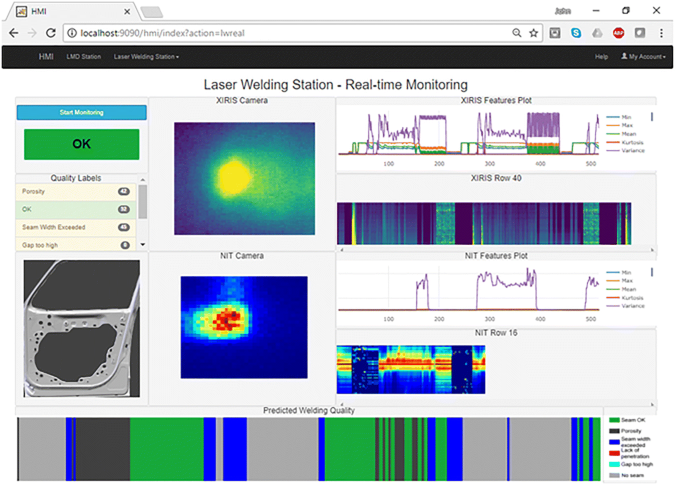

  

  Web-based platform’s functionalities (real-time)

• Data post processing and feedback: The third function offers to the user the capability to load information of welds occurred in previous products/stitches while a visible assessment can be performed providing feedback and retraining the classification model. In addition, the profile of each stitch, the quality color code, the features plot, and the defect counter are also incorporated and visualized. The stitch profile allows the operators to obtain conclusions for any critical defect such as lack of fusion and burnt areas. Such screens are demonstrated in Fig. 9.

  Fig. 9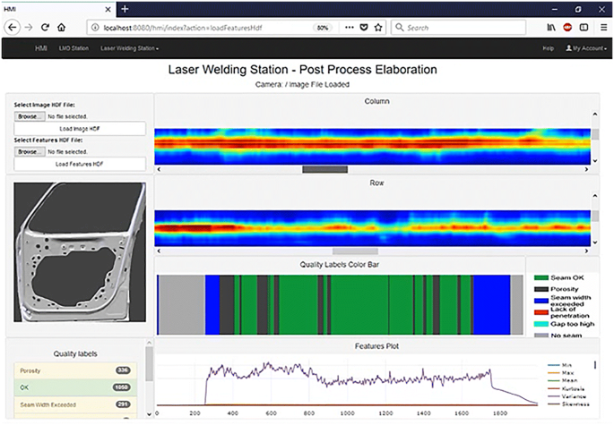

  

  Web-based platform’s functionalities (post-process)

Results & discussion

Using the developed feature extraction algorithms, one can derive interesting results regarding the defect’s identification. As depicted in Fig. 10, almost all the defects can be identified and show differences with the ideal thermal field. The method is only hindered by the vertical (coaxial to camera) cracks. However, this is depending on the crack’s size with the bigger ones to be as identifiable as the rest. On the other hand, Fig. 11 demonstrates that the Geometrical Feature Extraction algorithm can predict and visualize the difference in the size of the cracks while the numerical value can be a future threshold for accepting or rejecting the monitored weld.

Fig. 10

Cracks identification based on variance

Fig. 11

Cracks size identification

As far as it concerns the results related to the weld porosity, the Geometrical Feature Extraction algorithm can successfully identify its existence as presented in Fig. 12 as well as the position of the defects in relation to the center of laser beam as can also be detected in Fig. 13. Finally, in Fig. 14, the size identification capabilities of the algorithm can be seen.

Fig. 12

Identification of pores based on variance

Fig. 13

Pores position detection

Fig. 14

Porous size defect identification

For the prediction of the quality of parts, labeled measurements (images) were acquired [30], aiming to calculate the features of each frame, use the SVM classifier to predict the welding quality, and validate the method’s capacity to adequately work with new measurements. In this regard, the linear SVM was trained utilizing the “soft-margin optimization” formulation [40], with two welding data sets and the outcome of the prediction for a new trial can be achieved for each frame, labeled by the algorithm. It was observed that by using ten (10) principle components (Fig. 15) along with the two Geometrical Moments derived from the Geometrical Feature Extraction algorithm, quality prediction accuracy of 92%, on training and test data, was achieved. Afterwards, the same procedure was applied to more experimental trials for the prediction of the quality state of the two classes. The results of the classification are evident in Fig. 16 where specific centers of clusters are given for the sake of illustration.

Fig. 15

Cumulative sum of principal components

Fig. 16

Evaluation of classification model for two quality classes. Axes are values of two principal components and do not have particular physical substance

Considering the platform’s UI/HMI functionalities, as described briefly in the previous section, the quality assessment module along with statistical calculations introduced a number of operations to be integrated. In this regard, as depicted in Fig. 8, the maximum (Max), minimum (Min), Mean, Kurtosis, and Variance were calculated and plotted for each of the incoming image frames in real time. In addition, the Geometrical Feature Extraction algorithm’s defect identification and characterization capabilities, as mentioned in the previous paragraphs, introduce quality labels along the seam (Seam OK, Porosity, Seam width exceeded, lack of penetration, Gap too high). Finally, the overall seam quality was presented with a binary type indicator (“OK”, “NOK”) by engaging the complete quality assessment module. The same functionalities were introduced also in case of the post-processing elaboration mode (Fig. 9).

Concluding from aforementioned results, the mechanism which the defect’s development is based upon, as well as their correlation with the process’s emission, is fairly complex and not entirely deterministic and thus, the selection of ML models for predict/classify defects was made at the first place. These models have the advantage of built in error terms, where big amount of data is used to fit the model’s parameters based on its input-output response, offering error quantification and confident levels under significant lower computational requirements during their real-time utilization. The time references of the input and output variables are not bounded to single moment thus introducing prediction characteristic to the model. Nevertheless, defects occurring later, i.e., during cool down phase have not been taken into consideration and would require post-processing monitoring. However, the HMM algorithm could be elaborated to this end.

Conclusions and future work

In this paper, a novel web-based quality diagnosis platform has been presented. The lack of unified tools that are able to receive, process, and share quality data, is addressed through the proposed platform. The platform integrates a unified feature extraction, quality prediction, and decision-making algorithm by visualizing crucial aspects of laser processes that enable the operator’s feedback to the system. The current study regards the Laser Welding case; however, the platform can be easily adapted to accommodate the monitoring imaging systems of other applications, besides any training and validation, as mentioned in [7,8,9,10] extending by these means the cognitive capacity of the platform, such as additive manufacturing/laser metal deposition and cutting.

The algorithm and the platform’s performance have been locally validated with real data. The connection of the platform with the real monitoring system as well as a feasibility case for another laser process are the next steps to be undertaken by the authors to fully demonstrate the cognitive and networked capabilities of such a tool, in today’s production, aligned with the Industry 4.0 paradigm.

Challenges for the future, as isolated from the workflow above, include the fusion with other sensors (either mathematically or per use), the adaptive & robust control of the process which requires estimation of thermal field evolution within the part, dissimilar joining and respective metrics extraction, as well as adaptation of the current work-flow within a digital twin for more advanced functionalities.

References

Chryssolouris G (1991) Laser machining: theory and practice. Springer Science & Business Media.
Salonitis K, Stavropoulos P, Fysikopoulos A, Chryssolouris G (2013) CO 2 laser butt-welding of steel sandwich sheet composites. The International Journal of Advanced Manufacturing Technology 69(1–4):245–256. https://doi.org/10.1007/s00170-013-5025-7
Bikas H, Stavropoulos P, Chryssolouris G (2016) Additive manufacturing methods and modelling approaches: a critical review. The International Journal of Advanced Manufacturing Technology 83(1-4):389–405. https://doi.org/10.1007/s00170-015-7576-2
Stavropoulos P, Stournaras A, Salonitis K, Chryssolouris G (2010) Experimental and theoretical investigation of the ablation mechanisms during femptosecond laser machining. International Journal of Nanomanufacturing 6(1-4):55–65. https://doi.org/10.1504/IJNM.2010.034772
Mourtzis D, Vlachou E (2018) A cloud-based cyber-physical system for adaptive shop-floor scheduling and condition-based maintenance. Journal of Manufacturing Systems 47:179–198. https://doi.org/10.1016/j.jmsy.2018.05.008
Stavridis J, Papacharalampopoulos A, Stavropoulos P (2018) Quality assessment in laser welding: a critical review. The International Journal of Advanced Manufacturing Technology 94(5-8):1825–1847. https://doi.org/10.1007/s00170-017-0461-4
Leung CLA, Marussi S, Atwood RC, Towrie M, Withers PJ, Lee PD (2018) In situ X-ray imaging of defect and molten pool dynamics in laser additive manufacturing. Nature Communications 9(1):1–9. https://doi.org/10.1038/s41467-018-03734-7
Nommeots-Nomm A, Ligorio C, Bodey AJ, Cai B, Jones JR, Lee PD, Poologasundarampillai G (2019) Four-dimensional imaging and quantification of viscous flow sintering within a 3D printed bioactive glass scaffold using synchrotron X-ray tomography. Materials Today Advances 2:100011. https://doi.org/10.1016/j.mtadv.2019.100011
Qi L, Yi H, Luo J, Zhang D, Shen H (2020) Embedded printing trace planning for aluminum droplets depositing on dissolvable supports with varying section. Robotics and Computer-Integrated Manufacturing 63:101898. https://doi.org/10.1016/j.rcim.2019.101898
Yi H, Qi L, Luo J, Zhang D, Li N (2019) Direct fabrication of metal tubes with high-quality inner surfaces via droplet deposition over soluble cores. Journal of Materials Processing Technology 264:145–154. https://doi.org/10.1016/j.jmatprotec.2018.09.004
Günther J, Pilarski PM, Helfrich G, Shen H, Diepold K (2016) Intelligent laser welding through representation, prediction, and control learning: an architecture with deep neural networks and reinforcement learning. Mechatronics 34:1–11. https://doi.org/10.1016/j.cirp.2016.04.072
Galantucci LM, Tricarico L, Spina R (2000) A quality evaluation method for laser welding of Al alloys through neural networks. CIRP Annals - Manufacturing Technology 49(1):131–134. https://doi.org/10.1016/j.mechatronics.2015.09.004
Alexopoulos K, Makris S, Xanthakis V, Sipsas K, Chryssolouris G (2016) A concept for context-aware computing in manufacturing: the white goods case. International Journal of Computer Integrated Manufacturing 29(8):839–849. https://doi.org/10.1080/0951192X.2015.1130257
Pastras G, Fysikopoulos A, Giannoulis C, Chryssolouris G (2015) A numerical approach to modeling keyhole laser welding. The International Journal of Advanced Manufacturing Technology 78(5-8):723–736. https://doi.org/10.1007/s00170-014-5668-z
Fortunato A, Guerrini G, Melkote SN, Bruzzone AAG (2015) A laser assisted hybrid process chain for high removal rate machining of sintered silicon nitride. CIRP Annals - Manufacturing Technology 64(1):189–192. https://doi.org/10.1016/j.cirp.2015.04.033
Günther J, Pilarski PM, Helfrich G, Shen H, Diepold K (2014) First steps towards an intelligent laser welding architecture using deep neural networks and reinforcement learning. Procedia Technology 15:474–483. https://doi.org/10.1016/j.protcy.2014.09.007
Bautze T, Diepold K, Kaiser T (2009) A cognitive approach to monitor and control focal shifts in laser beam welding applications. Intelligent Computing and Intelligent Systems 2:895–899. https://doi.org/10.1109/ICICISYS.2009.5358247
Zhang Y, Gao X, Katayama S (2015) Weld appearance prediction with BP neural network improved by genetic algorithm during disk laser welding. Journal of Manufacturing Systems 34:53–59. https://doi.org/10.1016/j.jmsy.2014.10.005
Mayr A, Lutz B, Weigelt M, Gläßel T, Kißkalt D, Masuch M, Franke J (2018) Evaluation of machine learning for quality monitoring of laser welding using the example of the contacting of hairpin windings. In 2018 8th International Electric Drives Production Conference (EDPC) (pp. 1-7). IEEE. https://doi.org/10.1109/EDPC.2018.8658346
You D, Gao X, Katayama S (2014) WPD-PCA-based laser welding process monitoring and defects diagnosis by using FNN and SVM. IEEE Transactions on Industrial Electronics 62(1):628–636. https://doi.org/10.1109/TIE.2014.2319216
Lee J, Bagheri B, Kao HA (2015) A cyber-physical systems architecture for industry 4.0-based manufacturing systems. Manufacturing Letters 3:18–23. https://doi.org/10.1016/j.mfglet.2014.12.001
Mourtzis D, Vlachou E (2016) Cloud-based cyber-physical systems and quality of services. The TQM Journal 28(5):704–733. https://doi.org/10.1108/TQM-10-2015-0133
García-Díaz A, Panadeiro V, Lodeiro B, Rodríguez-Araújo J, Stavridis J, Papacharalampopoulos A, Stavropoulos P (2018) OpenLMD, an open source middleware and toolkit for laser-based additive manufacturing of large metal parts. Robotics and Computer-Integrated Manufacturing 53:153–161. https://doi.org/10.1016/j.rcim.2018.04.006
Stavridis J, Papacharalampopoulos A, Stavropoulos P (2018) A cognitive approach for quality assessment in laser welding. Procedia CIRP 72:1542–1547. https://doi.org/10.1016/j.procir.2018.03.119
Purtonen T, Kalliosaari A, Salminen A (2014) Monitoring and adaptive control of laser processes. Physics Procedia 56:1218–1231. https://doi.org/10.1016/j.phpro.2014.08.038
Rogalski A (2010) Infrared detectors. CRC press
Schmidt M, Otto A, Kägeler C (2008) Analysis of YAG laser lap-welding of zinc coated steel sheets. CIRP Annals 57(1):213–216. https://doi.org/10.1016/j.cirp.2008.03.043
Nasrabadi NM (2007) Pattern recognition and machine learning. Journal of Electronic Imaging 16(4):049–901. https://doi.org/10.1117/1.2819119
Dagum P, Galper A, Horvitz E (1992) Dynamic network models for forecasting. In Proceedings of the eighth international conference on uncertainty in artificial intelligence. Pp. 41-48.
Zenodo MAShES community: https://zenodo.org/communities/mashes/?page=1&size=20. Accessed April 25th 2019
Song F, Guo Z, Mei D (2010) Feature selection using principal component analysis. IEEE: System science, engineering design and manufacturing informatization 1:27–30. https://doi.org/10.1109/ICSEM.2010.14
fdesign.notch:https://www.mathworks.com/help/dsp/ref/fdesign.notch.html?w.mathworks.com. Accessed April 25th 2019
Furumoto T, Ueda T, Alkahari MR, Hosokawa A (2013) Investigation of laser consolidation process for metal powder by two-colour pyrometer and high-speed video camera. CIRP Annals - Manufacturing Technology 62(1):223–226. https://doi.org/10.1016/j.cirp.2013.03.032
Guo W, Liu Q, Francis JA, Crowther D, Thompson A, Liu Z, Li L (2015) Comparison of laser welds in thick section S700 high-strength steel manufactured in flat (1G) and horizontal (2G) positions. CIRP Annals - Manufacturing Technology 64(1):197–200. https://doi.org/10.1016/j.cirp.2015.04.070
SO 5817 (2014) https://www.iso.org/standard/54952.html.
Trogh J, Plets D, Martens L, Joseph W (2015) Advanced real-time indoor tracking based on the Viterbi algorithm and semantic data. International Journal of Distributed Sensor Networks 11(10):271818–271811. https://doi.org/10.1155/2015/271818
Mourtzis D, Vlachou E, Milas N, Xanthopoulos N (2016) A cloud-based approach for maintenance of machine tools and equipment based on shop-floor monitoring. Procedia CIRP 41:655–660. https://doi.org/10.1016/j.procir.2015.12.069
Papacharalampopoulos A, Stavropoulos P, Stavridis J, Chryssolouris G (2016) The effect of communications on networked monitoring and control of manufacturing processes. Procedia CIRP 41:723–728. https://doi.org/10.1016/j.procir.2015.12.041
Papacharalampopoulos A, Stavridis J, Stavropoulos P, Chryssolouris G (2016) Cloud-based control of thermal based manufacturing processes. Procedia CIRP 55:254–259. https://doi.org/10.1016/j.procir.2016.09.036
Cristianini N, Shawe-Taylor J (2000) An introduction to support vector machines and other kernel-based learning methods. Cambridge University Press, Cambridge
Acknowledgments
The dissemination of results herein reflects only the authors’ view and the Commission is not responsible for any use that may be made of the information it contains.
Funding
This work is partially supported by the EU Project AVANGARD. This project has received funding from the European Union’s Horizon 2020 research and innovation program under grant agreement No. 869986.
Author information
Authors and Affiliations
Corresponding author
Additional information
Publisher’s note
Springer Nature remains neutral with regard to jurisdictional claims in published maps and institutional affiliations.
Rights and permissions
Open Access This article is licensed under a Creative Commons Attribution 4.0 International License, which permits use, sharing, adaptation, distribution and reproduction in any medium or format, as long as you give appropriate credit to the original author(s) and the source, provide a link to the Creative Commons licence, and indicate if changes were made. The images or other third party material in this article are included in the article's Creative Commons licence, unless indicated otherwise in a credit line to the material. If material is not included in the article's Creative Commons licence and your intended use is not permitted by statutory regulation or exceeds the permitted use, you will need to obtain permission directly from the copyright holder. To view a copy of this licence, visit http://creativecommons.org/licenses/by/4.0/.
About this article
Cite this article
Stavropoulos, P., Papacharalampopoulos, A., Stavridis, J. et al. A three-stage quality diagnosis platform for laser-based manufacturing processes. Int J Adv Manuf Technol 110, 2991–3003 (2020). https://doi.org/10.1007/s00170-020-05981-9
Received:
Accepted:
Published:
Issue Date:
DOI: https://doi.org/10.1007/s00170-020-05981-9