
Abstract
Modeling of fluid flows in density-based topology optimization forms a longstanding challenge. Methods based on the Navier–Stokes equations with Darcy penalization (NSDP equations) are widely used in fluid topology optimization. These methods use porous materials with low permeability to represent the solid domain. Consequently, they suffer from flow leakage in certain areas. In this work, the governing equations for solid/fluid density-based topology optimization are reevaluated and reinterpreted. The governing equations are constructed using the volume averaged Navier–Stokes (VANS) equations, well known in the field of porous flow modeling. Subsequently, we simplify, interpret and discretize the VANS equations in the context of solid/fluid topology optimization, and analytically derive lower bounds on the Darcy penalization to sufficiently prevent flow leakage. Based on both the NSDP and VANS equations, two flow solvers are constructed using the Finite Volume method. Their precision and the lower bound on the Darcy penalization are investigated. Subsequently, the solvers are used to optimize flow channels for minimal pressure drop, and the resulting designs and convergence behavior are compared. The optimization procedure using the VANS equations is found to show less tendency to converge to inferior local optima for more precise flow solutions and is less sensitive to its parameter selection.
1 Introduction
Optimization of flow-related problems is a challenging yet highly relevant subject. Topology optimization has been successfully applied to such problems as can be found in the extensive literature survey by Alexandersen and Andreasen (2020). In fluidic topology optimization, the two most popular approaches are density-based and level-set based optimization. In the first work on density-based fluidic topology optimization by Borrvall and Petersson (2003) the distinction between the fluid and solid parts of the design domain is introduced using an inverse permeability. They optimize 2D channel flow between two plates where in the solid domain the two plates are close to eachother, resulting in low permeability and limited flow. Low permeability is modeled by adding a high penalization on the flow. In the fluid domain the two plates are further apart, permeability is high and only a low penalization on the flow is added. Design variables control a penalization on the flow, and thus influencing permeability of the domain. This approach leads to a set of governing equations that combines the Darcy flow problem with the Stokes equations and is only suitable for low Reynolds flow. Subsequently, Gersborg-Hansen et al. (2005) extend this framework from Stokes to Navier–Stokes flow by including inertia terms. Furthermore, they note that the reference to flow between two plates can be dropped and replaced by flow through a porous medium modeled by a Brinkman-type model (Brinkman 1949). We will refer to the resulting set of equations as the Navier–Stokes equations with Darcy penalization (NSDP equations).
Kreissl et al. (2011) found that density-based optimization using the NSDP equations required specific stabilization procedures and solutions suffered from erroneous “pressure diffusion” trough the solid domains. Kreissl et al. (2011) use pressure diffusion to refer to pressure gradients in the solid domain which drive erroneous flow in these domains. In this work we will refer to this effect as “flow leakage“, as we will argue that fluid pressure gradients in the porous “solid” domain should be expected and flow through this domain is representative of both flow and pressure field errors in the fluid domain. As a solution to these density-based optimization problems, Kreissl and Maute (2012) propose to use level-set based optimization using X-FEM. In contrast, level-set based fluid optimization allows for crisp solid/fluid boundaries and rigorously diminishes spurious flow through solid parts of the design domain. Provided, if combined with a suitable modeling approach (Kreissl and Maute 2012) use X-FEM). There is however no such thing as a free lunch as resulting designs may become more dependent on the initial guess of the level-set function, as shown by Allaire et al. (2004). However, topological derivatives can be used to measure the effect of adding solid islands in the fluid domains, alleviating the influence of the initial design on the optimum (Challis and Guest 2009; Guillaume and Idris 2004). A disadvantage of current topological derivatives is that only solid material can be added in the flow domain, but the effect of creating a channel between two separate flow domains cannot be assessed using topological derivatives to the best of the authors’ knowledge. The pressure gradients and flow leakage in the solid design domain in density-based optimization can thus also be seen as an advantage. They distribute sensitivities throughout the entire design domain and carry information on the effect of creating a channel between two separate flow domains as noted by Alexandersen and Andreasen (2020). However, similar to level set-based methods, density-based methods will also converge to local optima dependent on initial design and optimization parameters. Although the more restricted design modifications of the level-set approach result in a stronger dependence on the initial design.
Methods which blend features of level set-based and density-based approaches are proposed by Li et al. (2022), Picelli et al. (2022) and Behrou et al. (2019). To attain sensitivity information in the solid domain Li et al. (2022) optimize a topology based on a level set function while representing the solid domain as highly impermeable porous material. They thus do not enforce no flow penetration through the solid/fluid interface but inhibit solid domain flow using a penalization. The biggest advantage of this method is the fact that a body-fitted mesh may be used to accurately capture surface effects and no continuation approach is required for the flow penalization. However, using the level set approach other optimization parameters are introduced which also influence design convergence. Picelli et al. (2022) represent the topology using a crisp interface and explicitly prescribe no-penetration conditions on the solid/fluid interface such that no flow is present in the solid domain. Moreover, sensitivities in the fluid domain are computed by assuming porous material and a flow penalization may be introduced in the fluid domain (but in practice porous regions are not present in the flow computation). Subsequently, spatial filtering is used to populate the solid regions with sensitivities. However, the extrapolation of sensitivities into the solid regions is dependent on a spatial filtering radius and therefore parts of the solid domain will not contain any sensitivities. Similarly, Behrou et al. (2019) use a density-based model and remove flow in the solid domain by adaptive removal/addition of elements with a density below a certain threshold value. Both these last two methods have the additional advantage of reducing the computational cost of solving the physics. However, a disadvantage of these methods is that sensitivity information is also removed in the large solid areas. Consequently, the effect of adding channels in solid domains cannot be measured, creating difficulties for the optimizer to add these kind of design features. Both level-set and density-based flow optimization thus have their advantages and disadvantages. In this paper, we use density-based fluidic topology optimization as we prefer its natural ability to add islands to the fluid domain and create channels in the solid domain. Furthermore, we aim to improve the flow model such that errors caused by flow leakage are reduced.
Several authors have already studied variations on the porous flow model to increase its precision and reduce flow leakage. A mixed formulation of the Darcy–Stokes equations is implemented by Guest and Prévost (2006), and they note the similarity between their flow model and the Brinkman equation for flow through multiple scale porous media. Contrary to Borrvall and Petersson (2003) who find some intermediate density elements at the solid/fluid boundaries of their optimal designs due to a density filter which is applied to prevent convergence to inferior local optima, Guest and Prévost (2006) find crisp solid/fluid optimal designs. They argue that their methods automatically converge to discrete valued designs and apply a continuation strategy on the maximum flow penalization and a procedure of smoothing/projecting the design variables to prevent convergence to inferior local optima. Furthermore, they note the possibility to use the new method to optimize porous/fluid structures. However, the mixed Darcy–Stokes equations only consider Stokes flow in the fluid domain and do not include the inertial effects in the Navier–Stokes equations. Philippi and Jin (2015) and Alonso and Silva (2021) extend the standard NSDP equations by including a Forchheimer permeability tensor besides the Darcy penalization to penalize flows. The Forchheimer permeability tensor, derived in detail by Whitaker (1996), adds a porous drag at higher Reynolds numbers which scales quadratically with flow velocities. Alonso and Silva (2021) found improved designs when the Forchheimer tensor was included.
Further extensions to the NSDP equations can be found in the optimization of permeable microstructures. Governing equations in these optimizations allow for flow through the porous domain and are interesting to investigate from the perspective of solid/fluid optimization where the porous domain approaches a solid. A unit cell within a larger periodic porous medium is optimized in micro scale using a standard Brinkman type model by Guest and Prévost (2007). Subsequently, a more refined Darcy penalization is computed for the NSDP equations using homogenization techniques similar to the techniques which will be used in this work. Takezawa et al. (2020) extend this work by also computing the Forchheimer permeability tensor. Furthermore, Michaël et al. (2020) use the method of volume averaging to derive state equations for the modeling and optimization of spatially varying porous media. Volume averaging is a well-known technique in the field of flow modeling, used to construct refined porous flow models. Moreover, by including a high flow penalization in the porous domain, distinct solid/fluid designs are found in the results computed by Michaël et al. (2020). Extended and more accurate porous flow models have thus been investigated in the context of topology optimization. However, these techniques have not been applied to the construction and interpretation of flow models particularly for solid/fluid topology optimization.
In most previous topology optimization studies, porous flow models based on the Darcy or Brinkman equations were used to define solid/fluid parts in the design domain. Robustly decreasing flow leakage and finding correct interpolation functions for material properties remains a challenge in fluidic topology optimization (Alexandersen and Andreasen 2020)). However, as discussed in the previous paragraphs, more extensive porous flow models exist and can be used in topology optimization (Alonso and Silva 2021; Michaël et al. 2020)). To improve robustness of the optimization procedure and gain a better understanding of the equations for fluidic topology optimization, we approach the porous flow model from a more general viewpoint. An extended set of governing equations is investigated which we interpret and discretize specifically for solid/fluid topology optimization. Particularly, we will use the concept of volume averaging to derive the volume averaged Navier–Stokes (VANS) equations following Whitaker (1969, 1996). By closely examining and interpreting the VANS equations, we aim to improve two of the challenges set by Alexandersen and Andreasen (2020): improve “precision of solution and/or optimality”, improve “parameter robustness and algorithmic stability”.
In topology optimization we want to divide a design domain into a fluid and solid (impermeable porous) part using a single set of continuous governing equations to represent the flow everywhere within the design domain. The governing set of equations should thus be able to accurately capture both flow near the solid/fluid interface as well as in the solid and fluid domains. Accurately modeling of flows near porous/fluid interfaces has long been a subject of research, and is relevant for optimized flow structures where the porous/fluid interface represents a solid/fluid interface. A boundary condition was proposed by Beavers and Joseph (1967) to account for a jump in stress at the interface and to couple the Stokes to Poiseuille flow in a porous/fluid channel. Ochoa-Tapia and Whitaker (1995) propose a momentum jump condition for the interface based on the VANS equations to couple the Brinkman flow model to the Stokes flow model. Many authors discussed the nature of the jump in stress at the porous/fluid interface, continuity of stress, velocity and pressure, and appropriate governing equations/boundary condition (Nield 1991; Vafai and Kim 1995; Goyeau et al. 2003; Valdés-Parada et al. 2007). More recent studies by Breugem and Boersma (2005) and Hernandez-Rodriguez et al. (2022) compared pore scale simulations with volume averaged simulations and found matching results when the VANS equations were used. Furthermore, Hernandez-Rodriguez et al. (2022) confirm the necessity to include the Brinkman corrections to accurately model flow at the porous/fluid interface. In this work we will draw inspiration from these papers to be able to accurately capture stresses at the solid/fluid interface, and use volume averaged equations to improve solution precision.
Summarizing, the main contributions of this paper are the following:
-
1.
For a solid/fluid topology optimization problem a refined flow model is constructed by investigating the limit case of the VANS equations where porous material represents a solid. This method improves design convergence for optima with similarly precise flow solutions as optima obtained using the NSDP equations.
-
2.
Lower bounds on the Darcy penalization will be derived analytically such that flow leakage in the solid domain is limited, improving parameter robustness of the optimization problem.
This paper is structured as follows: Sect. 2 gives an introduction to volume averaging techniques for self-containedness, shows the VANS equations and compares them to the standard NSDP equations. Section 3 presents the discretization of the VANS equations, and the interpolation function used to dicretize the Darcy penalization. Subsequently, we derive lower bounds on the Darcy penalization in Sect. 4, and make an a priori estimation of flow leakage. In Sect. 5 the optimization problem and a method for adjoint sensitivity computations are presented. In Sect. 6 we compare precision of the flow solution based on the VANS and NSDP equations for a range of Darcy penalizations and Reynolds numbers. Section 7 performs structural optimization using both the VANS and NSDP equations and compares the resulting structures in terms of precision and objective. Finally, in Sect. 8, we draw conclusions on the use of the VANS equations for topology optimization and identify subjects for further research.
2 The volume averaged Navier–Stokes equations
In this section a recap of the derivation of the VANS equations following Whitaker (1996; Ochoa-Tapia and Whitaker 1995) is given, such that we are able to appropriately implement them in topology optimization. Subsequently, the limits of the VANS equations and their suitability for solid/fluid optimization are investigated. Moreover, the VANS equations are simplified and used to derive the NSDP equations.
2.1 A short introduction to the volume average
The aim of fluidic topology optimization is to divide design domain \(\Omega\) into a solid and a fluid domain such that an optimal material layout is found for a certain objective and set of constraints. For density-based solid/fluid optimization, we simulate the solid domain as an impermeable porous domain and simulate flow using the VANS equations. The concept of a volume average is introduced using the porous and fluid domains \(\Omega_{\rm p}\) and \(\Omega_{\rm f}\) respectively, as shown in Fig. 1. The domains have interface \(\Gamma_{\rm fp} = \overline{\Omega }_{\rm f} \cap \overline{\Omega }_{\rm p}\), where \(\overline{\square }\) denotes the closure of a domain. For each \(\pmb{x}\) an averaging domain \(\Omega_{\rm a}\) is defined as depicted in Fig. 2. The averaging domain is centered around \(\pmb{x}\) where vector \(\pmb{y}\) points to locations within the averaging domain. Furthermore, it has volume V and contains solid \(\beta\) and fluid \(\phi\). Consequently, the domain can be split into its fluid part (\(\Omega_\phi\) with volume \(V_\phi\)) and solid part (\(\Omega_\beta\) with volume \(V_\beta\)) as \(\Omega_{\rm a} = \Omega_\phi \cup \Omega_\beta\), and the interface between these domains is defined as \(\Gamma_{\phi \beta } = \overline{\Omega }_\phi \cap \overline{\Omega }_\beta\).

Design domain \(\Omega\) divided into a fluid domain \(\Omega_{\rm f}\) and a porous domain \(\Omega_{\rm p}\), both domains are connected at boundary \(\Gamma_{\rm fp} = \overline{\Omega }_{\rm f} \cap \overline{\Omega }_{\rm p}\). Centered around all \(\pmb{x}\) an averaging domain \(\Omega_{\rm a}\) is defined as illustrated in Fig. 2
To find the average of property \(\Psi\) in fluid phase \(\phi\) at coordinates \(\pmb{x}\) the intrinsic (\(\langle \Psi \rangle^{i\phi }_{\pmb{x}}\)) and superficial (\(\langle \Psi \rangle^{s\phi }_{\pmb{x}}\)) volume averages are defined as:
where \(\pmb{y}\) is used to integrate over fluid domain \(\Omega_\phi\) centered around \(\pmb{x}\). Both the intrinsic and superficial averages are thus field quantities dependent on coordinate \(\pmb{x}\), for convenience the subscript \(\pmb{x}\) is omitted in the remainder of this work. Using the superficial volume average the volume fraction of phase \(\phi\) is defined as:
which is used to relate the two averages as \(\langle \Psi \rangle^{s\phi } = \alpha_\phi \langle \Psi \rangle^{i\phi }\). The difference in interpretation between the superficial and intrinsic averages can be explained using the volume fraction. The superficial average represents the bulk average and should generally converge to zero as \(\alpha_\phi \rightarrow 0\), whereas the intrinsic average represents the pore scale average within the fluid domain and does not necessarily converge to zero as \(\alpha_\phi \rightarrow 0\). For example, if within a certain averaging volume the fluid has constant pressure \({p} = p_{\rm c}\) and the volume fraction approaches zero, the intrinsic average will be \(\langle p \rangle^{i\phi} = p_{\rm c}\), but the superficial average will also approach zero \(\langle p \rangle^{s\phi} = \alpha_\phi \langle p \rangle^{i\phi} \rightarrow 0\).

An averaging volume centered around \(\pmb{x}\), containing solid phase \(\beta\) and fluid phase \(\phi\). The averaging domain \(\Omega_{\rm a}\) can be divided into two parts as \(\Omega_{\rm a} = \Omega_\phi \cup \Omega_\beta\), where the interface between the two parts is \(\Gamma_{\phi \beta } = \overline{\Omega }_\phi \cup \overline{\Omega }_\beta\) at which a normal \(\pmb{n}_\phi\) is defined pointing to phase \(\beta\). The porous microstructure has characteristic length \(l_\phi\), and the averaging domain has characteristic length \(r_0\). Vector \(\pmb{y}\) is used to integrate over an averaging domain fixed at location \(\pmb{x}\)
Subsequently, some useful mathematical relations are defined. The volume average of a gradient can be simplified using the averaging theorem (Howes and Whitaker 1985):
where \(\Gamma_{\phi \beta }\) is the interface between phases \(\phi\) and \(\beta\) within \(\Omega_{\rm a}\) and \(\pmb{n}_\phi\) is the unit normal pointing outward of phase \(\phi\) on this interface, as shown in Fig. 2. Moreover, the averaging theorem in combination with the definition of the volume fraction can be used to prove that:
Finally, we assume that fluid field quantities can be split into their averaged and a deviational part as:
where \(\tilde{\Psi }\) is the deviation from the average which is small compared to \(\langle \Psi \rangle^{i\phi }\). Furthermore, for the averages we assume that:
For these approximations to be valid for the pressure or velocity of a fluid, separation of scales is required (Whitaker 1969). If \(l_\phi\) and \(r_0\) are the characteristic length of the porous microstructure and averaging volume, respectively, as shown in Fig. 2, separation of scales for quantity \(\Psi\) requires that:
where \(L_\Psi\) is a characteristic length of property \(\Psi\) defined by:
These conditions ensure that Eq. 6 holds and may furthermore be used to define the average of the deviation as:
Using these tools and properties, the VANS equations can be defined in a meaningful manner, where only relatively simple closure relations are required to solve the resulting equations. We furthermore note that the introduced concepts for volume averaging show many similarities with the homogenization concepts for topology optimization in (Hassani and Hinton 1998), and the averaging concepts for turbulent flow as shown in Alfonsi (2009).
2.2 Derivation of the VANS equations
In this section, the general VANS equations are presented, such that they can be interpreted and simplified for topology optimization in the coming sections. Whitaker (1996) and Ochoa-Tapia and Whitaker (1995) derive the VANS equations starting from the incompressible Navier–Stokes equations, consisting of the continuity equation and momentum equations, respectively:
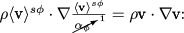
where \(\rho\) and \(\mu\) are the density and kinematic viscosity, p the fluid pressure and \({\pmb{\text{v}}}^\intercal = [u, v, w]\) is the velocity field where u, v, w are the velocities in Cartesian coordinate directions x, y, z, respectively. Subsequently, the VANS equations are derived by taking the superficial volume average of the Navier–Stokes equations:
A derivation of the averaged continuity equation is found in (Ochoa-Tapia and Whitaker 1995) and shown in Appendix 1, resulting in:
The superficial velocity field is thus solenoidal and is divergence-free in contrast to the intrinsic velocity field which has to satisfy:
where we used the relation between superficial and intrinsic averages \(\langle \pmb{\text{v}} \rangle^{s\phi } = \alpha_\phi \langle \pmb{\text{v}} \rangle^{i\phi }.\) We prefer to solve for the superficial flow field as this will simplify the required solution procedure. Subsequently, we focus our attention on the averaging of the more complex momentum equations. For the derivation of the left-hand side of the averaged momentum equation we refer the reader to Whitaker (1996), and for the derivation of the right-hand side we refer to Ochoa-Tapia and Whitaker (1995), resulting in:
where separation of scales is already used to simplify the equations. Whereas the superficial flow average is used, the VANS equations use the intrinsic pressure average for reasons explained in Sect. 2.3. For the interested reader, an example of the derivation of the averaged continuity equation and viscous forces is given in Appendix 1. In the coming section, an interpretation and simplification of the VANS equations will be given. The simplification and interpretation will follow results from literature, and are aimed at building a better understanding of the VANS equations in the context of topology optimization.
2.3 Interpretation of the VANS equations for solid/fluid topology optimization
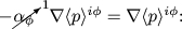
The VANS equations have many terms which have different physical origins. Closely inspecting these terms helps in using the VANS equations for topology optimization. Firstly, we focus on terms containing deviational velocities (\(\tilde{\pmb{\text{v}}}\)) and pressures (\(\tilde{p}\)), as we do not want to solve for them and want to remove them from the equations. The boundary integral in Eq. 14 is investigated:
In (Whitaker 1996) this term is referred to as the surface filter, as it filters information from the microscale solid/fluid interface to the averaged scale. To form a closure relation to interpret this term, Whitaker (1996) notes that at interface \(\Gamma_{\phi \beta }\) the velocity \(\pmb{\text{v}} = \langle \pmb{\text{v}} \rangle^{i\phi } + \tilde{\pmb{\text{v}}} = \pmb{0}\) and thus:
Subsequently, Whitaker (1996) uses this idea to construct a relation between the deviational and averaged quantities:
where \(\pmb{m}\) and \(\pmb{M}\) are a vector and matrix, respectively, used to relate averaged to deviational quantities and close the VANS equations. By inserting these approximations in the surface filter, it may be simplified as:
where the intrinsically averaged velocity is substituted with the superficially averaged velocity. Whitaker (1996) goes into great detail to define \(\pmb{K}\), but for the purpose of this work we recognize it as the Darcy’s law permeability tensor. Furthermore, the permeability tensor is simplified as \(\pmb{K} = \kappa \pmb{I}\) by assuming isotropy of the porous medium and the tensor is recognized as the penalization used in the NSDP equations for topology optimization to inhibit flow through solid domains. Moreover, Whitaker (1996) defines the order of magnitude for the Darcy permeability tensor as:
Choosing the correct magnitude for \(\kappa\), such that flow through the solid domain is inhibited sufficiently in an optimization procedure, remains a challenge. However, in Sect. 4 an order analysis will be used to derive lower bounds on \(\mathcal{O}\left( \kappa \right)\) which will result in lower bounds of similar form as Eq. 19.
Another interesting term in the momentum equation is the so called volume filter (Whitaker 1996):
which filters information from the flow on microscale to the macroscale. This is actually similar to the Reynolds stress tensor used in the Reynolds Averaged Navier Stokes (RANS) equations for turbulent flow modeling (Alfonsi 2009). In this work we will neglect this term as we assume the deviational velocities to be small, and remain within the laminar flow regime:
Moreover, adding this term for RANS optimization might not be straightforward. In the RANS equations velocity fluctuations \(\tilde{\pmb{\text{v}}}\) stem from local eddies which are filtered out via a time average, whereas in the laminar VANS equations velocity fluctuations \(\tilde{\pmb{\text{v}}}\) stem from flow interaction at the pore scale solid/fluid interface.
Subsequently, we investigate the viscous terms in the averaged momentum equations:
where the first part is called the Brinkman correction and the second part the second Brinkman correction (Ochoa-Tapia and Whitaker 1995; Brinkman 1949). In an optimized solid/fluid design flow in “solid” porous regions is generally limited and \(\nabla^2\langle \pmb{\text{v}} \rangle^{s\phi } \rightarrow 0\). The Brinkman correction is thus mainly important in the fluid regions. In contrast, the second Brinkman correction is mainly important in boundary regions where large gradients in volume fraction \(\nabla \alpha_\phi\) are found. In solid/fluid topology optimization the aim is to create crisp 0-1 designs where a porous “solid” region of low permeability (\(\alpha_\phi \rightarrow 0\)) is adjacent to a fluid region (\(\alpha_\phi =1\)). In the boundary regions the second Brinkman correction should thus be included. However, according to Whitaker (1986) a solid wall should not be approximated using the second Brinkman correction as the length scale of the averaging volume \(r_0\) becomes of the same order as the length scales of \(\alpha_\phi\) and \(\langle \pmb{\text{v}} \rangle^{i\phi }\) and we cannot adhere to the separation of scales. One of the solutions to this problem is to use a two domain approach in which separate governing equations are defined for the homogeneous fluid and solid domains. Subsequently, these equations are coupled via a jump condition on the solid/fluid interface concerning velocities and shear stresses (Beavers and Joseph 1967; Ochoa-Tapia and Whitaker 1995; Angot et al. 2017). However, Breugem and Boersma (2005) and Hernandez-Rodriguez et al. (2022) show that flow along a porous wall can be accurately simulated using the VANS equations including the second Brinkman correction using a correct interpretation of the results and a correct definition of the permeability tensor. As we want to optimize the solid/fluid layout within the design domain and do not know the solid/fluid domains a priori, we prefer to use only the VANS equations and not use a two domain approach.
A physical interpretation of the second Brinkman correction for solid/fluid topology optimization is given using Fig. 3. In the derivation of the VANS equations in Appendix 1 the correction shows up as a simplification of a surface integral over the microscale solid/fluid interface \(\Gamma_{\phi \beta }\):
In Fig. 3 we show an averaging volume on porous/fluid interface \(\Gamma_{\rm fp}\) where the porous material approaches a solid \(l_\phi \rightarrow 0\). In the "solid" porous domain flow speeds and gradients within the pores are negligible with respect to flow speeds within the fluid domain. Within the averaging volume we may thus neglect the surface integral over porous domain boundaries \(\Gamma_{\phi \beta } \setminus \Gamma_{\rm fp}\) and simplify the boundary integral as:
Moreover, if the formulation is taken to its limits where the porous material is a solid and \(l_\phi =0\), it is clear that \(\Gamma_{\phi \beta } = \Gamma_{\rm fp}\) and Eq. 24 holds. Furthermore, the momentum equation (and its volume average) represent an equilibrium between mass flow acceleration and stresses on an small domain of fluid. Subsequently, the boundary integral over \(\Gamma_{\rm fp}\cap \Gamma_{\phi \beta}\) is interpreted as an average of the viscous stresses (\(\mu \nabla \langle \pmb{\text{v}} \rangle^{i\phi }\)) on the solid/fluid interface. Within the averaging domain, these stresses are supported by the solid material at the interface. Supporting a part of these stresses by a rigid solid material thus reduces mass flow acceleration and consequently flow. The second Brinkman correction thus represents the support of fluid domain viscous stresses by the solid material at the porous/fluid interface. Moreover, if these fluid domain viscous stresses would not be supported by the solid material, they would have to be be supported by the fluid in the porous domain. The second Brinkman correction can thus be said to remove fluid domain viscous forces from flow in the porous domain.

An illustration of the effect of the second Brinkman correction on porous/fluid interface \(\Gamma_{\rm fp}\). Within the pores flow magnitude is small with respect to flow magnitude in the fluid domain. Fluid domain viscous forces are subsequently mainly supported by the solid material at \(\Gamma_{\rm fp}\)
Subsequently, we interpret the inertial term on the left-hand side of Eq. 14:
where we simplified \(\langle \pmb{\text{v}} \rangle^{s\phi }/ \alpha_\phi = \langle \pmb{\text{v}} \rangle^{i\phi }\). The inertial term on the right-hand side represents the advection of microscale momentum \(\rho \langle \pmb{\text{v}} \rangle^{i\phi }\) by bulk flow \(\langle \pmb{\text{v}} \rangle^{s\phi }\). The supposed advantage of this term in topology optimization is illustrated on a converged solid/fluid design. In topology optimization, the solid domain is defined by a low and constant volume fraction \(\alpha_\phi = \underline{\alpha } \ll 1\), resulting in:
Comparing the right-hand side of Eq. 26 to the standard inertial term in the Navier–Stokes equations \(\rho \pmb{\text{v}} \cdot \nabla \pmb{\text{v}}\) (as in Eq. 10), we notice that the density is divided by \(\underline{\alpha }\). The division by the volume fraction is interpreted as a scaling of density in the solid domain \(\rho^{\rm s} = \rho /\underline{\alpha } \gg \rho\), where “density” thus increases relative to the fluid domain where \(\alpha_\phi = 1\). As larger masses require higher forces to accelerate, this should reduce flow in the solid domain. However, in Sect. 4 we will argue and in Sect. 6 we will find that the effect of this term on flow reduction is small when solid/fluid laminar flow designs are evaluated. Nonetheless, we will keep this term in our optimization model as the work by Alonso and Silva (2021) who added the Forchheimer penalization besides the Darcy penalization suggests that a quadratic flow penalization improves designs found at higher Reynolds numbers. In this sense, the inertia term is interpreted as a quadratic flow penalization which passes information on inertial effects to the sensitivities.
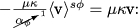
Finally, the new pressure term on the right-hand side of Eq. 14 is interpreted:
For the pressure field the intrinsic average is used, as the superficial pressure average (\(\langle p \rangle^{i\phi } = \langle p \rangle^{s\phi }/\alpha_\phi\)) leads to more complex equations:
Furthermore, in the standard momentum equation (as shown in Eq. 10), the pressure gradient \(-{\nabla p}\) represents the volumetric pressure forces acting on a parcel of fluid. However, in the VANS equations these forces are multiplied by the fluid volume fraction \(-\alpha_\phi \nabla \langle p \rangle^{i\phi }\). As the solid domain in topology optimization is defined as the domain where \(\alpha_\phi =\underline{\alpha } \ll 1\), pressure forces on a fluid parcel in this domain are reduced and \(\underline{\alpha }\nabla \langle p \rangle^{i\phi } \ll \nabla \langle p \rangle^{i\phi }\). Consequently, flow leakage caused by large pressure gradients in the solid domain is reduced. Moreover, if we assume that these pressure gradients are the main cause of flow leakage, the pressure penalization directly inhibits these errors in converged solid domains where \(\alpha_\phi \rightarrow 0\) while it does not add much penalization in intermediate designs with a lot of “gray” material where \(\alpha_\phi \approx 0.5.\) In fact, the pressure penalization will allow us to use a lower maximum Darcy penalization than the one required by the NSDP equations as will be shown in Sect. 6. The advantage of this lowered penalization is that intermediate designs containing a lot of gray material will be penalized less and the optimizer will be less restricted than when the NSDP equations are used with a larger maximum penalization.
Implementing the simplifications in Eqs. 18 and 21, the VANS momentum equation is simplified to:
where we thus used superficial velocity averages and intrinsic pressure averages. Furthermore, as might be obvious at this stage, we aim to use the VANS equations for topology optimization where volume fraction \(\alpha_\phi\) is used as a design variable.
2.4 Comparison to standard practice
The VANS equations show many similarities to the NSDP equations often used for fluid topology optimization:
where Darcy penalization \(\kappa\) is a function of the design variables. In the solid domain flow is inhibited by setting a large \(\kappa\) resulting in a high flow penalization \(-\mu \kappa \pmb{\text{v}}\), while in the fluid domain \(\kappa =0\) and Eq. 30 collapses to the standard Navier–Stokes equation (Eq. 10). If the NSDP equations are a simplification of the VANS equations, we can deduce that superficial velocity averages are used in the NSDP equations as the continuity equation is the same as the left-hand side of Eq. 13. Differences between the VANS and NSDP equations are found in the momentum equations. Rewriting the VANS (Eq. 29) to the NSDP (Eq. 30) equations can thus be done by assuming the velocity and pressure in the NSDP equations to be the superficial and intrinsic averages respectively (\(\langle \pmb{\text{v}} \rangle^{s\phi } = \pmb{\text{v}}\), \(\langle p \rangle^{i\phi } = p\)), and:
-
1.
 The second Brinkman correction is not included in the NSDP equations, and the support of fluid domain viscous stresses at the solid/fluid interface is removed.
 -
2.
 Volume fraction \(\alpha_\phi\) is removed from the inertia term, and its flow leakage reducing effect as illustrated by Eq. 26 and its influence on the sensitivities are removed.
 -
3.
 Flow leakage due to high pressure gradients in the solid domain is worsened as the volume fraction is removed from the pressure term.
 -
4.
 In the Darcy penalization, the division by \(\alpha_\phi\) is removed. However, in Sect. 3.1.4 we will show that using certain interpolation functions \(\kappa (\alpha_\phi )\), the Darcy penalization in the VANS and NSDP equations can be similar or the same.
 The second Brinkman correction is not included in the NSDP equations, and the support of fluid domain viscous stresses at the solid/fluid interface is removed.
 Volume fraction
  Flow leakage due to high pressure gradients in the solid domain is worsened as the volume fraction is removed from the pressure term.
 In the Darcy penalization, the division by
 The NSDP equations are thus a simplification of the VANS equations where we hypothesize that the VANS equations will be able to more precisely describe flow in an optimized solid/fluid topology. For the remainder of this work we will simplify notation by dropping the brackets and superscripts from the averaged variables and assuming that \(\pmb{\text{v}}\) is the superficial velocity average, p the intrinsic pressure average and \(\alpha\) the fluid volume fraction.
3 Discretization of the VANS equations
To use the VANS Equations in topology optimization, volume fraction \(\alpha\) is used as design variable. A well-known method to solve and discretize computational fluid dynamics (CFD) is the finite volume (FV) method, which is often preferred due to its natural ability to conserve mass and momentum. As the topology optimization community originated from the structural analysis community where the Finite Element Method (FEM) is the standard, most fluidic optimization papers use FEM. However, the structured square meshes often used in topology optimization are highly suited for discretization using the FV method, and fast solution algorithms exist for these kind of problems.
3.1 Discretized momentum equation
The VANS and NSDP equations are discretized using the FV method and solved using the Semi-Implicit Method for Pressure Linked Equations (SIMPLE) algorithm as described in Versteeg and Malalasekera (2007). The NSDP equations are discretized following Versteeg and Malalasekera (2007), with an exception for the Darcy penalization which is discretized in Sect. 3.1.4. In this section we first show the VANS discretization as several terms in the VANS equations are not standard in a CFD analysis. Furthermore, in this work we only consider 2D problems where we neglected flow w in the z-direction.
The VANS equations are discretized on an equidistant staggered grid as shown in Fig. 4, where different control volumes are used for the continuity (p-control), u-momentum and v-momentum equations. Subsequently, Eq. 29 is split into u/v-momentum equations as:
where we assumed solutions to be static (\(\partial u/ \partial t = \partial v/\partial t = 0\)), and spatial derivatives are written as \(p_{,x} = \partial p/ \partial x\) and \(p_{,y} = \partial p/ \partial y\). Only the discretization of the u-momentum equations is described since the discretization of the v-momentum equation is analogous. To discretize the u-momentum equation we use control volume (CV) \(\Omega_u\), as shown in Fig. 5. The CV has boundary \(\Gamma_u = \overline{\Omega }_u {\setminus } \Omega_u = \Gamma^N \cup \Gamma^E \cup \Gamma^S\cup \Gamma^W\), where the superscripts denote north, east, south and west boundaries. Design variables representing volume fractions within the cells are attached to the red pressure nodes in Fig. 5, we however interpolate these variables on the north/south edges of the CV and at the center of the CV (at DOF \(u^{\rm P}\) in Fig. 5):
where all design variables on the right-hand sides can be found in Fig. 5. Furthermore, v-velocities on the north/south edges are interpolated as:
To discretize the u-momentum equation it is integrated over its control volume:
In the subsequent sections first the inertial pressure and viscous terms will be discretized after which more attention is given to the second Brinkman correction and Darcy penalization, finally the discretization is finished by discretizing the continuity equation.

The staggered equidistant grid used to discretize the VANS equations using the FV method. velocity DOFs (green arrows) are located at the cell faces, while pressure DOFs and design variables are located at the cell centers (red dots). Design variables \(\alpha\) are attached to the cell centers and represent a constant volume fraction within the corresponding cell, as illustrated by the upper right cell which is solid and where \(\alpha \rightarrow 0\). Different control volumes are defined for the u, v momentum equations, and the continuity (p) equation. At the u-control volume all neighboring DOFS contributing to the momentum equation are depicted in Fig. 5. (Color figure online)

Control volume \(\Omega_u\) for the u-momentum equation. We denote the relevant DOFs and design variabels with respect to the center DOF \(u^{\rm P}\). The boundary of the control volume is divided into horizontal boundaries \(\Gamma^N\) and \(\Gamma^S\) with length \(\Delta x\), and vertical boundaries \(\Gamma^E\) and \(\Gamma^W\) with length \(\Delta y\)
3.1.1 Discretized inertial, pressure and viscous terms
The inertial term is discretized by applying the divergence theorem on the CV:
where we used the continuity equation (\(\nabla \cdot \pmb{\text{v}} = 0\)) to rewrite \(\pmb{\text{v}} \cdot \nabla \frac{u}{\alpha } = \nabla \cdot \left( \pmb{\text{v}} \frac{u}{\alpha } \right)\) and \(\pmb{n}_u\) is the unit normal pointing outward of \(\Omega_u\) on \(\Gamma_u\). We discretize the inertial terms using approximations on the north, south and east, west boundaries, respectively:
where \(\Delta x\) and \(\Delta y\) are the horizontal and vertical lengths of the control volume as in Fig. 5. In the discretized term, intrinsic momentum \(\rho u/\alpha\) is advected through the boundaries by superficial flow average \(\pmb{\text{v}}\). If momentum is to be conserved, advection of inertial momentum through a CV boundary should be consistent for all adjacent CV’s. The intrinsic momentum \(\rho u/\alpha\) and superficial flow \(\pmb{\text{v}}\) on a certain boundary should thus be the same for both elements adjacent to the boundary. As \(\pmb{\text{v}}\) and u are already interpolated consistently for all elements on the boundaries, volume fractions \(\alpha^{CN}\) and \(\alpha^{CS}\) are also interpolated consistently in Eq. 32 at the north and south boundaries.
The pressure term is discretized by approximating the gradient in pressure and \(\alpha\) at the center of the CV:
To discretize the first Brinkman correction, the divergence theorem is used:
Subsequently, flow gradients are approximated on the north, south and east, west boundaries as:
Most of the discretization techniques used until this point are fairly common and can be found in Versteeg and Malalasekera (2007). However, in most common methods fluid volume fraction \(\alpha\) is not included, and in its inclusion and interpolation we deviate from most standard discrete CFD solvers.
3.1.2 Second Brinkman correction on a wall orthogonal to the flow
Special attention is given to the second Brinkman correction as it is not common in a standard FV discretization. The second Brinkman correction in Eq. 22 depends on the gradient in volume fraction \(\nabla \alpha\), and is used to support fluid domain viscous forces as explained in Sect. 2.3. The second Brinkman correction is investigated for a converged design where there are distinct regions of solid (\(\alpha \rightarrow 0\)) and fluid (\(\alpha = 1\)) material. In such a solid/fluid design, the gradient \(\nabla \alpha = [\alpha_{,x}~ \alpha_{,y}]^\intercal\) is only present on the porous/fluid interface (the solid wall), and is a vector normal to the interface pointing to the fluid domain. The two parts of the gradient \(\alpha_{,x}\) and \(\alpha_{,y}\) are investigated separately. In fact, the case where only \(\alpha_{,y}=0\) represents a vertical wall orthogonal to u as shown in Fig. 6, and the case where only \(\alpha_{,x}=0\) represents a horizontal wall parallel to u as shown in Fig. 7. The correction is thus split into a vertical and horizontal component:

The relevant DOFs and design variables for the discretization of the second Brinkman correction in the CV for \(u^{\rm P}\). In this example, the elements to the left are solid (\(\alpha^{W} \rightarrow 0\)), the elements to the right are fluid (\(\alpha^E=1\)), and \(\alpha_{,y}=0\) resulting in a vertical wall
Firstly, the correction is constructed for the vertical wall in Fig. 6, orthogonal to flow u in x-direction. The volume fraction is only dependent on x and the gradient in x-direction at the center of the CV is approximated as:
where \(\alpha^E\), \(\alpha^W\) are the east and west volume fractions as in Fig. 6. Subsequently, the gradient in \(u/\alpha\) at the center of the CV is approximated as:
where \(\alpha^{\rm P}\) is the volume fraction at \(u^{\rm P}\) as in Eq. 32. Using Eqs. 41 and 42, the second Brinkman correction for a vertical wall orthogonal to the flow direction is discretized as:

The last term in the second Brinkman correction works in the opposite direction of the Darcy penalization \(-\mu \kappa u/\alpha\) in Eq. 34. This term will be neglected as it is assumed to be small compared to the Darcy penalization which will be discretized in Eq. 60 and whose lower bound will be defined in Sect. 4, resulting in:
We investigate the correction for the vertical wall in Fig. 6 where \(\alpha^E=1\), \(\alpha^W \rightarrow 0\) resulting in \(\alpha^{\rm P} \approx 0.5\) and:
If the correction is combined with the viscous forces on east boundary \(\Gamma^E\) in Eq. 39:
we find that the second Brinkman correction removes these forces from the control volume as \(B_o^E + F_\mu^E \approx 0\). The second Brinkman correction thus removes the viscous forces due to fluid flow to the east where no porous material is present (\(\alpha^E = 1\)). This is exactly the goal of adding it as these forces are in fact supported by the solid material in the porous domain as explained in Sect. 2.3.
3.1.3 Second Brinkman correction on a wall parallel to the flow
In Sect. 3.1.2 the second Brinkman correction for flow orthogonal to a wall is investigated and explicitly discretized. However, horizontal walls parallel to u also contribute to the second Brinkman correction. As an example, we investigating the horizontal wall in Fig. 7 where \(\alpha^{\rm P}=1\) and \(\alpha^{\rm PN} \rightarrow 0\). A mismatch in the exact location of the wall is found. If the wall is interpreted as the boundary where flow stagnates, this leads to an interface at either \(y=\Delta y\) (\(u^N\rightarrow 0\)) or at \(y=\Delta y /2\) (\(v^{\rm NE} \rightarrow 0\) and \(v^{\rm SE} \rightarrow 0\)). Furthermore, for approximating gradients \(u_{,y}\) on \(\Gamma^N\) in Eq. 39, we approximated the velocity profile as:
resulting in a flow of \(u(y=\Delta y/2) = \frac{u^{\rm P} + u^N}{2}\) at north edge \(\Gamma^N\), which coincides with the wall where flow should be stagnant.

The relevant DOFs and design variables for the discretization of the second Brinkman correction in the CV for \(u^{\rm P}\). In this example, the elements to the north are solid (\(\alpha^{\rm PN}\rightarrow 0\)), the elements in the CV are fluid (\(\alpha^{\rm P}=1\)), and \(\alpha_{,x}=0\) resulting in a horizontal wall which coincides with the north edge of the CV \(\Gamma^N\)
In this case, a better approximation of the flow at \(\Gamma^N\) would be \(u^N\) as it should tend to zero. If opposed to Fig. 7\(\alpha^{\rm P}\rightarrow 0\) and \(\alpha^{\rm PN}=1\) and the porous domain is to the south of the wall at \(\Gamma^N\) instead of to the north, it follows that \(u^{\rm P}\rightarrow 0\) is a better approximation of the velocity at the wall at \(\Gamma^N\). Based on these requirements a new velocity interpolation is constructed on \(0\le y < \frac{\Delta y}{2}\):
which has a complementary interpolation on \(\frac{\Delta y}{2} < y \le \Delta y\):
A plot of the resulting flow fields is shown in Fig. 8. When \(\alpha^{\rm P}=\alpha^{\rm PN}\) no wall is present at \(\Gamma^N\) and Eqs. 48 and 49 collapse into Eq. 47. Moreover, as \(\alpha^{\rm P}\) and \(\alpha^{\rm PN}\) remain continuous variables, we are able to continuously introduce solid walls in a topology optimization procedure.

Two different flow fields for a vertical wall. Either the top elements are solid (\(\alpha^{\rm PN}\rightarrow 0\)) and the flow at \(\Delta y /2\) is approximated as \(u^N\rightarrow 0\), or the bottom elements are solid (\(\alpha^{\rm P}\rightarrow 0\)) and the flow at \(\Delta y /2\) is approximated as \(u^{\rm P}\rightarrow 0\)
Furthermore, the new flow fields for walls at \(\Gamma^N\) is accompanied with a flow field for walls at \(\Gamma^S\) on \(0\ge y > -\frac{\Delta y}{2}\):
Using these interpolation functions, the correct gradients at the boundaries are computed as:
The new gradient at the north edge contains a standard linear part (also found in Eq. 39 at \(\Gamma^N\)):
as well as an update (found by subtracting the gradient in Eq. 52 from the gradient in Eq. 51):
Subsequently, we define the correct viscous force at the north edge in Eq. 39 by using \(u_{,y}^c = u_{,y}^l + \Delta u_{,y}\) as:
from which we extract an update to the standard viscous forces by subtracting the viscous force at the north edge in Eq. 39 from Eq. 54:
Moreover, we find the update to have precisely the function of the Second Brinkman correction as described in Sect. 2.3. When we are investigating flow in the porous domain (\(\alpha^{\rm P}\rightarrow 0\)) with large viscous forces due to flow in a fluid domain above (\(\alpha^{\rm PN} = 1\)), the update becomes:
which can be subtracted from the standard viscous force at \(\Gamma^N\) in Eq. 39 (which is the viscous force due to \(u^l_{,y}\)):
to find that for this porous control volume the viscous forces at the north edge become \(B_{\rm p}^N +F_\mu^N \approx 0\). The function of the second Brinkman correction is to remove viscous forces in the fluid domain from the solid domain which is exactly what the update does. Consequently, we apply the second Brinkman correction for flow parallel to a wall using the updated velocity gradients in Eq. 51 instead of explicitly discretizing Eq. 40. Furthermore, the full correction for flow parallel to a wall is found by following a similar procedure on the south edge as:
Subsequently, the complete second Brinkman correction can be defined by combining Eqs. 44 and 58 as \(B_2 = B_o + B_{\rm p}\).
3.1.4 Discretized Darcy penalization
The final term which is discretized in the volume averaged momentum equation is the Darcy penalization:
where we introduce \(K(\alpha )\) as the design dependent penalization interpolation which will be used to compare different types of interpolation functions and maximum penalization in the solid domain (\(\overline{K} = K(\alpha =0)\)). The same discretization of the Darcy penalization will be used for both the VANS as well as the NSDP equations. Lower and upper bounds on \(\kappa\) are defined as \(\overline{\kappa } \ge \kappa \ge \underline{\kappa }=0\), which we relate to the volume fraction \(0<\alpha <1\) via a linear interpolation as \(\kappa (\alpha ) = (1-\alpha )\overline{\kappa }\). As one of the aims of the discretization is to introduce the least amount of tunable parameters for optimization, a linear interpolation is used to reduce complexities and parameters in the resulting discrete flow model. Subsequently, we approximate the penalization at the center of the CV by discretizing as:
In the limit case where \(\alpha^{\rm P} = 0\), i.e. fully solid, this would result in an infinitely large penalization which is computationally infeasible. To prevent this we add a lower bound \(\underline{\alpha } \ll 1\) on the volume fraction as \(\tilde{\alpha } = \underline{\alpha } + (1-\underline{\alpha })\alpha\) and use \(\tilde{\alpha }\) in the discretization such that \(\alpha^{\rm P} \ge \underline{\alpha }\).
In the work by Borrvall and Petersson (2003) and many subsequent papers on fluid topology optimization the Darcy penalization is interpolated as:
where \(\tilde{q}\) is a parameter which is used to control convexity, generally by setting it as \(0\le \tilde{q}\le 1\). This convex function ensures that the penalization on intermediate designs where \(\alpha \approx 0.5\) is not too severe, as a severe penalization on intermediate designs generally tends to pull the designs into local optima. In this work, no additional interpolation functions or filters are applied to \(\tilde{\kappa }\), besides the linear interpolation \(\kappa (\tilde{\alpha })=(1-\tilde{\alpha })\overline{\kappa}\). However, we may examine the function in Eq. 60 as an interpolation function:
which is in fact the same function as the one proposed by Evgrafov (2005). Furthermore, when \(\tilde{\alpha } = \underline{\alpha } + (1-\underline{\alpha })\alpha\) is substituted into Eq. 62, we find:
where we assumed \(\underline{\alpha } \ll 1\) and \(1-\underline{\alpha } \approx 1\), and note that using this interpolation function we find a maximum penalization in the solid domain of:
Moreover, comparing Eqs. 63 and 61 we note that they scale as \(\underline{\alpha }\cdot K_{\rm Su}(\alpha ) = K_{\rm Da}(\alpha)\) if \(\underline{\alpha } = \tilde{q} \ll 1\) and \(\mu \bar{\kappa } = \overline{K}_{\rm Da}\), as shown in Fig. 9. Under these assumptions, interpolation function \(K_{\rm Su}(\alpha )\) thus has the same shape as \(K_{\rm Da}(\alpha )\) but increases the overall Darcy interpolation as \({K_{\rm Su}(\alpha ) = K_{\rm Da}(\alpha )/\underline{\alpha } \gg K_{\rm Da}(\alpha )}\). A more severe penalization on intermediate designs where \(\alpha \approx 0.5\) is thus imposed using the discretization in Eq. 60, which is however balanced by defining a precise lower bound on \(\bar{\kappa }\) to sufficiently penalize flow in the solid domain in Sect. 4.

3.2 Discretized continuity equation
The continuity equation is needed to close the equations and is thus discretized on control volume \(\Omega_{\rm p}^c\) in Fig. 10 with boundary \(\Gamma_{\rm p}^c = \overline{\Omega }_{\rm p}^c {\setminus } \Omega_{\rm p}^c = \Gamma_{\rm p}^N \cup \Gamma_{\rm p}^E \cup \Gamma_{\rm p}^S \cup \Gamma_{\rm p}^W\). The continuity equation is integrated over the control volume and the divergence theorem is applied such that:
The continuity equation and its discretization are the same for both the VANS and NSDP equations.

The control volume \(\Omega_{\rm p}^c\) for the continuity equation with relevant DOFs, and boundary \({\Gamma_{\rm p}^c = \overline{\Omega }_{\rm p}^c {\setminus } \Omega_{\rm p}^c = \Gamma_{\rm p}^N \cup \Gamma_{\rm p}^E \cup \Gamma_{\rm p}^S \cup \Gamma_{\rm p}^W}\)
4 The Darcy penalization
The question of choosing the correct \(\bar{\kappa }\) is often a difficult one: setting it too low results in spurious flow through the solid domain while setting it too high may cause ill-convergence of the optimization procedure (Kreissl and Maute 2012). As a guideline the maximum penalization is often related to the Darcy number Da (Olesen et al. 2006):
where L is a characteristic length scale of the system. In porous flow modeling, the Darcy number represents the permeability of a porous medium and a low Darcy number is related to impermeable porous structures. Subsequently, it is stated that impermeable “solids” have low Darcy numbers \({\text{Da} \le 10^{-5}}\) which is used to define the inverse permeability of the solid \({\overline{K}={\upmu}L^{-2}\text{Da}^{-1}}\), and flow in the porous solid domain is penalized using Darcy penalization:
However, this leaves the question which length scale L to use in a changing topology. Using an inlet diameter may result in significantly lower \(\overline{K}\) than using the diameter of a narrow channel generated by the optimization procedure. Moreover, Darcy number Da is often either not low enough causing much flow leakage or too low resulting in inferior local optima and subsequently requires some tuning before optimization. We thus aim to define a lower bound on \(\bar{\kappa }\) to penalize flow in the solid domain sufficiently. In Sects. 4.1 and 4.2 the bounds will be derived for the VANS and NSDP equations respectively, after which Sect. 4.3 will give an overview and discussion of all derived bounds.

The intrinsic pressure field orthogonal to a horizontal wall which is at least \(C^1\)-continuous. For \({\Delta \rightarrow 0}\) the pressure gradient in the fluid (\(p^{\rm f}_{,y}\)) will thus approach the pressure gradient at the porous interface \({p^\Gamma_{,y}=p^{\rm f}_{,y}}\) at \(\Gamma_{\rm fp}\)
To define the lower bounds on the penalization, the horizontal solid/fluid interface \(\Gamma_{\rm fp}\) in Fig. 11 is investigated. Although a horizontal interface is used, the actual orientation of the interface is irrelevant to the derivation. On the interface, the pressure field is examined, where we remind the reader that we are actually dealing with the intrinsic pressure average \(\langle p \rangle^{i\phi }\). If we assume that \(\langle p \rangle^{i\phi }\) is a good representation and substitute of the actual pore scale pressure \(p^{pore}\), as stated by Eq. 5, we may relate properties of the averaged and pore scale pressures. Of the pore scale pressure field, we know that it is at least \(C^1\)-continuous, and assume this to also be the case for intrinsic pressure average \(\langle p \rangle^{i\phi }\). Subsequently, the pressure gradient orthogonal to the interface (\(p_{,y}\) for \(\Gamma_{\rm fp}\) in Fig. 11) is assumed to be at least \(C^0\)-continuous. In the remaining text we will return to the convention of writing intrinsic pressure average \(\langle p \rangle^{i\phi }\) as p, and superscripts \(\square^\Gamma\) and \(\square^{\rm f}\) will be used to denote porous quantities on the interface and quantities in the fluid domain respectively. Due to the continuity, the pressure gradient at porous fluid interface \(\Gamma_{\rm fp}\) (\(p_{,y}^\Gamma\)), and the gradient approaching \(\Gamma_{\rm fp}\) from the fluid domain (\(p_{,y}^{\rm f}\)) should thus be continuous at the interface (\(p_{,y}^\Gamma = p_{,y}^{\rm f}\) at \(\Gamma_{\rm fp}\)). Consequently, the order of these terms at \(\Gamma_{\rm fp}\) should be equal \({\mathcal{O}\left( p_{,y}^{\rm f}\right) =\mathcal{O}\left( p_{,y}^\Gamma \right) }\). An order of magnitude analysis will be performed on these terms to derive a lower bound on the order of magnitude of \(\bar{\kappa }\). To derive the bound, we aim to ensure no flow penetration at the solid/fluid interface \(\Gamma_{\rm fp}\).
4.1 Bounds on the Darcy penalization for the VANS equations
To derive the VANS bounds, firstly the VANS v-momentum equation found in Eq. 31 is used to define a general equation for \(p_{,y}\):
where Eq. 31 is reordered and divided by \(\alpha\) as it contains the pressure penalization \(\alpha p_{,y}\). Subsequently, we make the following assumptions to define \(p_{,y}^\Gamma\):
-
1.
The penalization at the interface is interpolate as \({\kappa^\Gamma = \bar{\kappa }(1-\alpha^\Gamma )}\).
-
2.
We assume the second Brinkman correction removes fluid domain viscous forces from the interface as explained and shown in Sects. 2.3, 3.1.2, 3.1.3, and thus neglect it and any contribution of fluid domain flow (\(v^{\rm f}\)) to the viscous forces at the interface.
Which results in a pressure gradient at the interface as:
Subsequently, we make the following assumptions to define \(p_{,y}^{\rm f}\):
-
1.
No flow penalization is applied in the fluid domain and \({\kappa^{\rm f} = 0}\).
-
2.
Fluid domain volume fraction \({\alpha^{\rm f}=1}\) is constant and thus \({\nabla \alpha^{\rm f} = 0}\).
Which results in a pressure gradient in the fluid domain as:
The magnitudes of the different terms in Eqs. 69 and 70 are related by performing an order analysis on the discretized equations. In the order analysis we approximate the magnitude of gradients as \({\mathcal{O}\left( \nabla \Psi \right) = \mathcal{O}\left( \Delta \Psi / \Delta x + \Delta \Psi / \Delta y\right) = \mathcal{O}\left( \Delta \Psi /h\right) }\) where \({h\approx \Delta x \approx \Delta y}\) is the element size. The magnitude of the gradient in the inertial term in Eq. 69 is thus approximated as:
where we used \({\Delta \alpha^\Gamma = 1}\) as we are investigating the porous/fluid (0/1) interface and approximate the flow magnitude using the flow itself \({\mathcal{O}\left( \Delta v^\Gamma \right) = \mathcal{O}\left( v^\Gamma \right) }\). Subsequently, the magnitude of the flow velocity is approximated as \({\mathcal{O}\left( \pmb{\text{v}}^\Gamma \right) = \mathcal{O}\left( \mid \pmb{\text{v}}^\Gamma \mid \right) \approx \mathcal{O}\left( u^\Gamma + v^\Gamma \right) }\), such that the magnitude of the inertial term in Eq. 69 can be approximated as:
Moreover, as there are no difficult terms present in the Darcy penalization in Eq. 69, its order is estimated as:
Diffusive terms are approximated as \({\mathcal{O}\left( \nabla^2\Psi \right) = \mathcal{O}\left( \Delta \Psi /\Delta x^2 + \Delta \Psi /\Delta y^2\right) = \mathcal{O}\left( \Delta \Psi /h^2\right) }\) such that the magnitudes of the viscous terms in Eqs. 69 and 70 are approximated as:
where we used \({\mathcal{O}\left( \Delta v^\Gamma \right) = \mathcal{O}\left( v^\Gamma \right) }\). Lastly, the inertial term in Eq. 70 is estimated along the same lines as Eq. 72:
where \({\mathcal{O}\left( \mid \pmb{\text{v}}^{\rm f} \mid \right) \approx \mathcal{O}\left( u^{\rm f} + v^{\rm f}\right) }\). The magnitudes of the flow at the porous interface/in the fluid domain are thus related by approximating the order of the pressure gradients using Eqs. 72, 73, 74, 75:
and by using continuity requirement \({\mathcal{O}\left( p_{,y}^{\rm f}\right) =\mathcal{O}\left( p_{,y}^\Gamma \right) }\):
To extract bounds on the penalization, an elemental Reynolds number is introduced to measure the respective relevance of the inertial and viscous forces as:
where we make the important note that it is dependent on mesh size h and not on characteristic length L. Two main cases are examined based on whether element scale viscous (\(\text{Re}^e \ll 1\)) or inertial (\(\text{Re}^e \gg 1\)) forces are dominant. Subsequently, bounds on the penalization will be constructed by aiming to stop flow from penetrating into the solid domain through the solid/fluid interface. We will quantify flow penetrating the interface relative to the flow in the fluid domain via flow reduction \({v^\Gamma /v^{\rm f}}\). If a relatively small amount of flow penetrates the interface, the order of the flow reduction becomes:
which will be used to derive bounds on \(\mathcal{O}\left( \bar{\kappa }\right)\).
4.1.1 VANS bounds: dominant viscous forces
If the viscous term is dominant (\(\text{Re}^e \ll 1\)), the inertial terms are neglected and Eq. 77 is simplified as:
where either the first or the second term on the left-hand side is dominant. If the first term \({(\mu v^\Gamma )/(\alpha^\Gamma h^2)}\) is dominant the main mechanism for flow reduction is the pressure penalization which causes the division by \(\alpha^\Gamma\) in Eq. 68. If the second term \({(\mu \bar{\kappa }(1-\alpha^\Gamma ) v^\Gamma )/({\alpha^\Gamma }^2)}\) is dominant the main mechanism for flow reduction is the Darcy penalization. We measure the relative dominance by dividing the first term with the second term:
and examine the two scenarios where either \({r_V^l>1}\) or \({r_V^l<1}\):
-
Dominant Darcy penalization (\(r_V^l<1\)):
If the second term on the left-hand side of Eq. 80 is dominant, the order analysis reduces to:
$$\begin{aligned} \mathcal{O}\left( \frac{\mu \bar{\kappa }(1-\alpha^\Gamma ) v^\Gamma }{{\alpha^\Gamma }^2}\right) = \mathcal{O}\left( \frac{\mu v^{\rm f}}{h^2}\right) , \end{aligned}$$(82)which is rewritten to find the flow reduction at the interface:
$$\begin{aligned} \mathcal{O}\left( \frac{v^\Gamma }{v^{\rm f}}\right) = \mathcal{O}\left( \frac{{\alpha^\Gamma }^2}{h^2\bar{\kappa }(1-\alpha^\Gamma )}\right) <1. \end{aligned}$$(83)The bound on the flow reduction is subsequently rewritten to find a lower bound on \(\bar{\kappa }\) for \({{\text{Re}}^e \ll 1}\) and \(r_V^l < 1\):
$$\begin{aligned} \mathcal{O}\left( \bar{\kappa }\right) > \mathcal{O}\left( \frac{{\alpha^\Gamma }^2}{h^2(1-\alpha^\Gamma )}\right). \end{aligned}$$(84) -
Dominant pressure penalization (\(r_V^l>1\)):
If the first term on the right-hand side of Eq. 80 is dominant, the order analysis reduces to:
$$\begin{aligned} \mathcal{O}\left( \frac{\mu v^\Gamma }{\alpha^\Gamma h^2} \right) = \mathcal{O}\left( \frac{\mu v^{\rm f}}{h^2} \right) , \end{aligned}$$(85)which can be rewritten to find the flow reduction as:
$$\begin{aligned} \mathcal{O}\left( \frac{v^\Gamma }{v^{\rm f}}\right) = \mathcal{O}\left( \alpha^\Gamma \right). \end{aligned}$$(86)Flow is thus automatically reduced for \({\alpha^\Gamma \ll 1}\) (\({\mathcal{O}\left( \alpha^\Gamma \right) } < 1\)) if the first term on the left-hand side of Eq. 80 is dominant.
4.1.2 VANS bounds: dominant inertial forces
In the second case, inertial terms are dominant (\(\text{Re}^e \gg 1\)) and the viscous forces can be neglected, resulting in:
where either the first or second term on the left-hand side is dominant. If the first term:
is dominant, the main mechanisms for flow reduction are the pressure penalization which causes the first division by \(\alpha^\Gamma\) in Eq. 68 and the inertial penalization which results in the \({(1-1/\alpha^\Gamma })\) term as can be seen in Eq. 71. If the second term \({(\mu \bar{\kappa }(1-\alpha^\Gamma ) v^\Gamma )/({\alpha^\Gamma }^2)}\) is dominant, the main mechanism for flow reduction is again the Darcy penalization. We measure the relative dominance by dividing the first term with the second term:
and again examine two scenarios where either \({r_V^h>1}\) or \({r_V^h<1}\):
-
Dominant Darcy penalization (\(r_V^h<1\)):
If the second term is dominant the order analysis reduces to:
$$\begin{aligned} \mathcal{O}\left( \frac{\mu \bar{\kappa }(1-\alpha^\Gamma ) v^\Gamma }{{\alpha^\Gamma }^2}\right) = \mathcal{O}\left( \frac{\rho \mid \pmb{\text{v}}^{\rm f} \mid v^{\rm f} }{h}\right) , \end{aligned}$$(90)which can be rewritten to find the flow reduction at the interface:
$$\begin{aligned}\mathcal{O}\left( \frac{v^\Gamma }{v^{\rm f}}\right)&= \mathcal{O}\left( \frac{\rho \mid \pmb{\text{v}}^{\rm f} \mid {\alpha^\Gamma }^2}{h\mu \bar{\kappa }(1-\alpha^\Gamma )} \right) \\&= \mathcal{O}\left( \frac{{\text{Re}}^e{\alpha^\Gamma }^2}{h^2\bar{\kappa }(1-\alpha^\Gamma )} \right) < 1, \end{aligned}$$(91)from which we can extract a bound on the penalization for \({{\text{Re}}^e \gg 1}\) and \(r_V^h < 1\) as:
$$\begin{aligned} \mathcal{O}\left( \bar{\kappa }\right) > \mathcal{O}\left( \frac{{\text{Re}}^e{\alpha^\Gamma }^2}{h^2(1-\alpha^\Gamma )} \right). \end{aligned}$$(92) -
Dominant pressure and inertial penalization (\(r_V^h>1\)):
If however the first term on the left-hand side of Eq. 87 is dominant the order analysis reduces to:
$$\begin{aligned} \mathcal{O}\left( \frac{\rho \mid \pmb{\text{v}}^\Gamma \mid v^\Gamma }{\alpha^{\Gamma }h}\left( 1 - \frac{1}{\alpha^\Gamma } \right) \right) = \mathcal{O}\left( \frac{\rho \mid \pmb{\text{v}}^{\rm f} \mid v^{\rm f} }{h} \right). \end{aligned}$$(93)The equation is subsequently rewritten to find that for \({\alpha^\Gamma \ll 1}\) flow at the interface is automatically lower than flow in the fluid domain:
$$\begin{aligned} \mathcal{O}\left( \frac{\mid \pmb{\text{v}}^\Gamma \mid v^\Gamma }{\mid \pmb{\text{v}}^{\rm f} \mid v^{\rm f}}\right) \approx \mathcal{O}\left( \frac{{v^\Gamma }^2}{{v^{\rm f}}^2}\right) = \mathcal{O}\left( \frac{\alpha^\Gamma }{1 - \frac{1}{\alpha^\Gamma }}\right) < 1. \end{aligned}$$(94)
For both Eqs. 86 and 94 we assumed that \({\alpha^\Gamma \ll 1}\) to achieve some flow reduction. In practice however, we use \(\alpha^\Gamma = \alpha^{\rm P} \approx 0.5\) which is just below 1. We will examine these assumptions and resulting errors in Sect. 4.4.
4.2 Bounds on the Darcy penalization for the NSDP equations
For the NSDP equations we can follow a similar procedure as for the VANS equations. In the fluid domain \(p_{,y}^{\rm f}\) is defined as in Eq. 70. In the porous domain \(p_{,y}^\Gamma\) is defined using Eq. 30 as:
where \(\kappa^\Gamma\) is interpolated using \({K_{\rm Su}(\alpha^\Gamma )}\) in Eq. 62. The orthogonal pressure gradient \(p_{,y}\) is again assumed to be continuous, and an order analysis is performed resulting in an equation similar to Eq. 77:
4.2.1 NSDP bounds: dominant viscous forces
If \(\text{Re}^e \ll 1\) and viscous forces are dominant inertial forces are neglected such that Eq. 96 reduces to:
We first examine the case where the first term on the left-hand side is dominant, resulting in:
which can be rewritten to find that no flow reduction takes place:
The only mechanism for flow reduction in the NSDP equations is thus the Darcy penalization and we assume that when an effective Darcy penalization is applied \(\mathcal{O}\left( v^\Gamma \right) < \mathcal{O}\left( v^{\rm f}\right)\) and we may neglect the first term on the left-hand side of equation 97:
After which the flow reduction:
is used to derive a lower bound on the penalization as:
4.2.2 NSDP bounds: dominant inertial forces
If \(\text{Re}^e\gg 1\) and inertial forces are dominant, the order analysis reduces to:
As was the case for low \(\text{Re}^e\), the only mechanism for flow reduction is the Darcy penalization and we neglect the first term on the left-hand side by assuming that \(\mathcal{O}\left( \mid \pmb{\text{v}}^\Gamma \mid v^\Gamma \right) < \mathcal{O}\left( \mid \pmb{\text{v}}^{\rm f} \mid v^{\rm f}\right)\), such that the inertial term at the interface can be neglected:
Subsequently, the analysis is again rewritten to find the order of flow reduction:
After which a lower bound on the Darcy penalization is defined as:
For the NSDP equations we thus derive bounds on the penalization under the assumption that flow reduction is a fact (\(\mathcal{O}\left( v^\Gamma \right) < \mathcal{O}\left( v^{\rm f}\right)\) and \(\mathcal{O}\left( \mid \pmb{\text{v}}^\Gamma \mid v^\Gamma \right) < \mathcal{O}\left( \mid \pmb{\text{v}}^{\rm f} \mid v^{\rm f}\right)\)). These assumptions however only hold when the appropriate penalization’s from Eqs. 105 and 102 are used. If these appropriate penalizations are not used there is no other mechanism for flow reduction and errors due to flow leakage will become large.
4.3 Overview and discussion of bounds on the penalization
Both the VANS and NSDP equations thus have bounds on the penalization dependent on the elemental Reynolds number as defined in Eq. 78. Moreover, the VANS equations may have an additional dependence on measurements \(r_V^l\) and \(r_V^h\) defined in Eqs. 81 and 89 which measure the dominant mechanism for flow reduction. We will first define bounds on the penalization assuming that the Darcy penalization is the dominant mechanism for flow reduction (\(r_V^l<1\) and \(r_V^h<1\)) resulting in the VANS bounds in Eqs. 84 and 92. In Sect. 4.4 we will come back to this assumption and show that although although the Darcy penalization is dominant the pressure penalization also plays a significant role in flow reduction. Subsequently, the VANS bounds in Eqs. 84 and 92 and NSDP bounds in Eqs. 102 and 106 are simplified by using the elemental Reynolds number \(\text{Re}^e\) and defining inverse elemental surface area:
resulting in the lower bounds on \(\mathcal{O}\left( \bar{\kappa }\right)\) as summarized in Table 1.
In practice for elements at the interface volume fraction \(\alpha^\Gamma = \alpha^{\rm P} \approx 0.5\) is used. In Table 1 the magnitudes depend on \(\alpha^\Gamma =0.5\) as \(\alpha^\Gamma /(1-\alpha^\Gamma )=1\) or \({\alpha^\Gamma }^2/(1-\alpha^\Gamma )=0.5\). For the order of magnitude the dependence on \(\alpha^\Gamma\) can thus be neglected resulting in the same penalization for the VANS and NSDP equations. Moreover, we require \(\bar{\kappa }\) to be an order of magnitude higher than the values in Table 1, and specify the increase in magnitude using \(10^q\), where q is a small whole number (generally \(q=0\), \(q=1\) or \(q=2\)). The resulting values which we implement for \(\bar{\kappa }\) can be found in Table 2.
To relate the maximum Darcy penalization found in this work to common practice we rewrite it as:
The maximum penalization in the solid domain at \(\alpha =\underline{\alpha }\) and \(\kappa =\bar{\kappa }\) for \({\text{Re}}^e\le 1\) is subsequently found as:
and for \({\text{Re}}^e > 1\) as:
where we treat \(10^q/\underline{\alpha }\) as a factor which scales the maximum penalization similar to the factor \(1/Da \gg 1\) which scales the commonly used maximum penalization by Olesen et al. (2006):
Comparing the maximum penalization for \({\text{Re}}^e\le 1\) in Eq. 110 to the common penalization in Eq. 111 they seem similar. However, whereas the common penalization is dependent on characteristic length L which may change for changing topologies, our new penalization is dependent on mesh size h which allows us to accurately predict errors as will be discussed in Sect. 4.4 and shown in Sect. 6. Moreover, the bounds for the Darcy penalization are also dependent on an elemental Reynolds number. This is not completely new as Kondoh et al. (2012) and Alexandersen et al. (2013) already implement a Reynolds dependent penalization. However, contrary to those works, the penalization in this work is dependent on an elemental Reynolds number and h instead of the global Reynolds number:
Whereas a global Reynolds number is computed using reference length L, the elemental Reynolds number in Eq. 78 is dependent on h which is often much lower (\(h\ll L\)) resulting in much lower elemental Reynolds numbers (\({\text{Re}}^e\ll {\text{Re}}\)). Moreover, the penalization definitions in Kondoh et al. (2012) and Alexandersen et al. (2013) are defined for non-dimensional Navier–Stokes equations which impacts their interpretation and comparision to common practice as discussed in Appendix 2.
We note that the elemental Reynolds number and thus the Darcy penalization remain dependent on an a priori estimate of \(\mid \pmb{\text{v}}^{\rm f}\mid\) which may cause problems in changing topologies when this estimate is erroneous. A solution to this problem could be a penalization dependent on actual local flow magnitude \(\mid \pmb{\text{v}}\mid\). However, as this requires the absolute flow magnitude this would introduce discontinuities in the gradients of the model used. Furthermore, this approach would be similar to the Forchheimer penalization introduced by Alonso and Silva (2021) who deal with discontinuous gradients by using automatic differentiation.
4.4 A priori error estimation
Using the bounds on the penalization as provided in the previous section, we may estimate flow leakage in the porous domain for low and high Reynolds flow. For low \({\text{Re}}^e \le 1\) we set \(\bar{\kappa } = 10^q H^e = 10^q h^{-2}\), which can be substituted into the estimated flow reduction at the interface in Eqs. 101 and 83, respectively:
when \(\alpha^\Gamma \approx 0.5\) at the solid/fluid interface. For the same value of q, flow at the interface should thus be reduced by a similar factor in the VANS as well as the NSDP equations. However, we speculate that the same flow reduction may also be used in the solid domain where \(\alpha \approx \underline{\alpha } \ll 1\):
for the NSDP and VANS equations, respectively, where \(v^{\rm s}\) represents the flow in the solid domain. Flow in the solid domain computed using the VANS equations may thus be decreased by an additional factor \(\underline{\alpha }\) with respect to the NSDP equations for low Reynolds flow. This stronger suppression of flow leakage originates from the penalization of the pressure gradient \(\alpha \nabla p\) in the VANS equations which added an extra division by \(\alpha\) in the definition of \(p_{,y}^\Gamma\) in Eq. 68. Furthermore, the estimates for flow reduction at the interface have been derived in Sects. 4.1 and 4.2, while the estimates in the porous domain are a speculation on the extensibility of Eq. 113. The extensibility of flow reduction in the porous domain is based on the idea that the pressure gradient should not only be continuous across the fluid domain and porous/fluid interface, but also across the porous/fluid interface and porous domain. Moreover, for high \({\text{Re}}^e > 1\) we set \({\bar{\kappa }} = 10^qH^e{\text{Re}}^e = 10^q{\text{Re}}^eh^{-2}\), which can be substituted into Eqs. 91 and 105 respectively resulting in the exact same flow reductions as in Eqs. 113 and 114.
If an insufficient penalization is chosen for the NSDP equations (\(q<0\)) flow leakage may introduce significant errors. However, for the VANS equations, there is still the possibility that \(r_V^l>1\) or \(r_V^h>1\) resulting in the Darcy penalization not being the dominant mechanism for flow reduction. The dominant mechanism for flow reduction is investigated by substituting \(\alpha^\Gamma \approx 0.5\) and \(\bar{\kappa }\) in Eqs. 81 and 89:
for \({\text{Re}}^e < 1\) (\(\bar{\kappa } = 10^q h^{-2}\)) and \({\text{Re}}^e>1\) (\({\bar{\kappa }} = 10^q{\text{Re}}^eH^e = 10^q \rho \left|\pmb{\text{v}}^{\rm f}\right|h^{-1} \mu^{-1}\)) respectively. In the low elemental Reynolds case, the dominant mechanism for flow reduction is thus completely determined by q. If \(q<0\) and as a result \(r_V^l>1\) we do not satisfy the condition for flow reduction through the Darcy penalization in Eq. 102, but still manage some flow reduction through the condition in Eq. 86:
This will not result in much flow reduction at the solid/fluid interface where \(\alpha^\Gamma \approx 0.5\). However, within the solid domain where \(\alpha = \underline{\alpha } \ll 1\) this flow reduction mechanism might have significant effects. To ensure sufficient flow penalization, in this work we will use \(q \ge 0\). If \({\text{Re}}^e>1,\) the problem is more complicated as the dominant mechanism for flow reduction depends on the flow reduction itself. However, if we substitute the flow reduction (\(\left|\pmb{\text{v}}^\Gamma \right|/\left|\pmb{\text{v}}^{\rm f}\right|\approx v^\Gamma /v^{\rm f}\)) due to the Darcy penalization in Eqs. 113 into \(r_V^h\) in Eq. 115 we find:
Similar to the low Reynolds case, if \(q<0\) it thus follows that the Darcy penalization is not the dominant flow reducing mechanism as \(r_V^h>1\). Moreover, flow at the interface is not reduced as substituting \(\alpha^\Gamma \approx 0.5\) into the flow reduction for \(r_V^h>1\) in Eq. 94 results in:
However, if we again speculate on the extensibility of these formulations to the porous domain where \(\alpha = \underline{\alpha }\ll 1\), we find a significant solid domain flow reduction of:
Finally, we make a note on the error in pressure, which is more difficult to estimate. In the solid domain, a non-zero pressure field will be present. However, the intrinsic average of the pressure field (\(\langle p \rangle^{i\phi }\)) is computed while the superficial average of the velocity field (\(\langle \pmb{\text{v}} \rangle^{s\phi }\)) is computed. When no fluid is pumped into the porous domain where \(\alpha \rightarrow 0\), velocity \(\langle \pmb{\text{v}} \rangle^{s\phi }\) naturally converges to zero, while \(\langle p \rangle^{i\phi }\) does not necessarily converge to zero as it represents the pore scale average as explained in Sect. 2. Non-zero intrinsic pressure fields in the solid domain should thus be expected and should not be treated as erroneous. Furthermore, for both the VANS and NSDP momentum equations, the pressure gradient at every point within the fluid domain can be written as solely a function of velocity: \(\nabla p = f(\pmb{\text{v}})\), if material properties \(\rho\), \(\mu\), \(\bar{\kappa }\) and \(\alpha =1\) are taken as constant. If the correct velocity field is found in the fluid domain, it follows that the correct pressure field is also computed, respective to a reference pressure in the fluid domain. As pressure gradients in the solid domain are expected, and errors in pressure are harder to quantify, we mainly focus on flow leakage as a representation of precision of the solution.
5 Optimization problem and adjoint sensitivity analysis
Using the discretization and bounds on the Brinkman penalization the optimization problem is defined as:
where N is the number of discrete design DOFs \(\alpha_i\), \(\pmb{R}(\pmb{u},\pmb{v},\pmb{p},\pmb{\alpha })\) is a column containing all discretized equilibrium equations, \(\pmb{u},~\pmb{v},~\pmb{p},~\pmb{\alpha }\) contain the discrete velocities pressures and design variables, the desired maximum fluid volume fraction is \(V_{\rm f}\) and \(f(\pmb{u},\pmb{v},\pmb{p},\pmb{\alpha })\) is the objective to be minimized. No additional filters such as a blurring filter or Heaviside projection are applied to the design as they are not necessary to regularize the optimization problems in this paper. The MMA algorithm by Svanberg (1987, 2004) is used to perform the optimization. Computing the sensitivities required by the MMA algorithm can be a cumbersome task in non-linear fluid problems. The main problem lies in the computation of the Jacobian matrix for the solution of the adjoint equations. In this work we use the MATLAB (2019) symbolic toolbox to construct discrete momentum and continuity equations, such that we are able to create functions for the Jacobian matrices before running the optimization. In essence, a similar approach as in (Dilgen et al. 2018) is implemented, where automatic differentiation is used to compute the Jacobian of the residuals.
To construct the adjoint sensitivities, columns containing discrete functions for the u, v-momentum and continuity equations are defined as \(\pmb{R}_u(\pmb{u},\pmb{v},\pmb{p},\pmb{\alpha })\), \(\pmb{R}_v(\pmb{u},\pmb{v},\pmb{p},\pmb{\alpha })\), \(\pmb{R}_{\rm p}(\pmb{u},\pmb{v},\pmb{\alpha })\) respectively. An element of \(\pmb{R}_u(\pmb{u},\pmb{v},\pmb{p},\pmb{\alpha })\) is thus associated with DOF \(u^{\rm P}\) and the stencil as in Fig. 5, where both \(u^{\rm P}\) and the stencil are mapped to the global mesh in Fig. 4. Boundary conditions are applied via ghost nodes as described in (Versteeg and Malalasekera 2007) and are added to the columns containing the discrete equations. All equations are gathered as \(\pmb{R}^\intercal = [\pmb{R}^{\intercal }_u, \pmb{R}^\intercal_v, \pmb{R}^\intercal_{\rm p} ]\) and \(\pmb{U} = [\pmb{u}^\intercal , \pmb{v}^\intercal , \pmb{p}^\intercal ]\). Furthermore, objective \(f(\pmb{u},\pmb{\text{v}},\pmb{p},\pmb{\alpha })\) is defined and used to construct the augmented objective:
where \(\pmb{\lambda }\) contains the adjoint multipliers. The sensitivities are subsequently defined as:
where first, the adjoint equations are solved:
after which the sensitivities are computed as:
The difficult part in solving the adjoint equations is to define \(\partial \pmb{R} / \partial \pmb{\alpha }\) and the Jacobian:
as it is never explicitly formed in the SIMPLE solution algorithm. We are however able to assemble the Jacobian after solving for flow and pressure fields, by using a symbolic coding toolbox. For example, element \(R_u^{i}\) of \(\pmb{R}_u\) contains the discretized u-momentum equation in terms of the symbolic stencil variables in Fig. 5\(\pmb{U}^{\rm s} = [u^{\rm P}, u^N, \ldots , v^{\rm NE}, \ldots \alpha^E, \ldots ]^\intercal\), and derivatives can be computed using symbolic differentiation \(\partial R_u^i/\partial \pmb{U}^{\rm s}\). As the derivatives for one stencil are the same for every element \(R_u^i\), we only perform the symbolic differentiation for one stencil and let the symbolic coding toolbox automatically construct a vector function from \(\partial R_u^i/\partial \pmb{U}^{\rm s}\) which takes vectors of DOFs \(\pmb{U}^{\rm s}\) and returns vectors of \(\partial R_u^i/\partial \pmb{U}^{\rm s}\). Both \(\pmb{U}^{\rm s}\) and \(\partial R_u^i/\partial \pmb{U}^{\rm s}\) can be mapped to the global mesh. The subsequent assembly procedure into \(\partial \pmb{R}/\partial \pmb{U}\) is coded by hand and the same procedure is performed for \(\partial \pmb{R} / \partial \pmb{\alpha }\). For this particular implementation, a symbolic toolbox which can compute derivatives and construct vector functions from symbolic equations is thus required. To confirm the adjoint sensitivities used in this work they are verified using complex step finite difference sensitivities in Appendix 3.
6 Precision of the VANS and NSDP Equations
A precise flow solution is essential for finding precise optima when optimizing fluid problems. The precision of the NSDP and VANS solvers is therefore investigated for several flow problems, Reynolds numbers, minimal volume fraction \(\underline{\alpha }\) and penalizations \(\bar{\kappa }\). As precision is of most importance in the optimal black/white designs, only these designs are investigated. In Appendix 4 we examine the effect of the second Brinkman correction and argue that flow leakage is a good measure for overall solution accuracy. Consequently, we will use flow leakage to asses solution precision in this section and the remainder of this work. To confirm the lower bound on \(\bar{\kappa }\) derived in Sect. 4 a sweep on power q is performed for low elemental Reynolds numbers (\(\text{Re}^e \le 1\)) in Sect. 6.1 and moderate elemental Reynolds flow (\(\text{Re}^e>1\)) in Sect. 6.2. The results in these sections will be used to choose optimization settings for q and \(\underline{\alpha }\) such that flow is sufficiently penalized in the optimization problems in Sect. 7. Flow is sufficiently penalized when we expect errors \(e^{\pmb{\text{v}}} \approx 10^{-1}\) and \(u_{\rm l} < 10^{-2}\). Error \(e^{\pmb{\text{v}}} \approx 10^{-1}\) is chosen relatively high on purpose as it represents a flow error in two cases and influences convergence behavior of the optimization procedure. The error is mainly caused by flow at those locations in the design where \(\alpha^{\rm P}\approx 0.5\), which are found at either the solid/fluid interface, or in the intermediate gray design during optimization where \(\alpha \approx 0.5\). If flow in the intermediate gray design is penalized too much, the optimizer can be pushed into an inferior local optimum from which it may be hard to escape. Moreover, when choosing the optimization settings we put more emphasis on \(u_{\rm l} < 10^{-2}\) as in Appendix 4 flow leakage is shown to correlate to errors in pressure drop (which we will optimize for in Sect. 7). Furthermore, in Sect. 6.3 the penalization for a range of Reynolds numbers is investigated.
6.1 Low elemental Reynolds numbers
First, a sweep on the penalization is performed for low \(\text{Re}^e\) (and low Re) using the problem depicted in Fig. 12 and the parameters given in Table 3. We examine a channel of height 2L where flow is obstructed by two solid porous walls of two elements thick. A parabolic flow profile with maximum velocity \(u_{\rm max}\) is prescribed at the inlet and pressure at the outlet is fixed at \(p_{\rm out}\). Furthermore, as equidistant meshes are used where \(\Delta x = \Delta y = h\) and four mesh refinements are examined where \(h=0.1\,L\), \(h=0.05\,L\), \(h=0.025\,L\), \(h=0.0125\,L\), the elemental Reynolds number can be computed as:
where \({\text{Re}}^e=h<1\) and we approximate \(\left|\pmb{\text{v}}^{\rm f} \right|\approx u_{\rm max}\). Since \({\text{Re}}^e=h<1\), the maximum \(\bar{\kappa }\) is computed following Table 2 as:
Furthermore, using the parameters in Table 3, the Reynolds number is computed as

A 2D channel with parabolic inflow applied at the left inlet and constant pressure applied at the right outlet. At \(L_{\rm wall}\) two small porous solid walls of thickness \(2\Delta x\) are inserted to inhibit flow. For different mesh sizes the problem will thus slightly vary as the wall thickness changes. For low Reynolds flow the wall affects the pressure distribution to the left and is placed at the center, while for moderate Reynolds flow the wall has large wakes to the right and is placed closer to the inlet

The errors \(e^{\pmb{\text{v}}}\) and \(u_{\rm l}\) for low \(\text{Re}^e\) in the problem as illustrated in Fig. 12 using the parameters from Table 3 computed using varying h and \(\underline{\alpha }\). The horizontal solid black lines indicate the maximum allowable errors \(e^{\pmb{\text{v}}} \approx 10^{-1}\) and \(u_{\rm l} < 10^{-2}\) for optimization, and are used to select appropriate optimization parameters q and \(\underline{\alpha }\)
To investigate the a priori error estimates in Sect. 4.4 the precision of the model is measured using a spurious flow error:
where \(I^p = \{i \mid (x_i,y_i) \in \Omega_{\rm p}\}\) denotes the indices i of all DOFs \(u_i, \;v_i\) in \(\Omega_{\rm p}\) and in this example the porous domain \(\Omega_{\rm p}\) consists of the two obstructing walls. Error \(e^{\pmb{\text{v}}}\) measures the norm of flow in the porous domain and at the porous/fluid interface, and normalizes it using a measure for flow in the fluid domain (\(u_{\rm max}\)). We expect flow at the porous/fluid interface to be dominant in the norm, and \(e^{\pmb{\text{v}}}\) can thus be seen as a measure for flow reduction \(v^\Gamma / v^{\rm f}\). Besides error \(e^{\pmb{\text{v}}}\) an error which represents the flow leakage in the solid domain is defined as:
where \(\Gamma_{\rm w}\) is the center line in the two walls as shown in Fig. 12. As \(u_{\rm l}\) represents the leakage in the porous wall where \(\alpha = \underline{\alpha}\) and is normalized by \(u_{\rm max}\), we use it as a measure of flow reduction in the solid domain \(v^{\rm s}/v^{\rm f}\). Both \(e^{\pmb{\text{v}}}\) and \(u_{\rm l}\) can thus be compared against the error estimates in Sect. 4.4.
6.1.1 Low elemental Reynolds results
Using these parameters the errors in Fig. 13 and the flow field in Fig. 14 are found. As shown in Fig. 13a and b, we generally find that \(\mathcal{O}\left( e^{\pmb{\text{v}}}\right) = \mathcal{O}\left( 10^{-q}\right)\) when \(q\ge 0\) which confirms the bounds on \(\bar{\kappa }\) in Sect. 4 and expected flow reduction \(v^\Gamma /v^{\rm f}\) in Eq. 113. Furthermore, for the NSDP equations in Fig. 13d \(\mathcal{O}\left( u_{\rm l}\right) = \mathcal{O}\left( \underline{\alpha } 10^{-q}\right)\) and for the VANS equations in Figure 13c \(\mathcal{O}\left( u_{\rm l}\right) = \mathcal{O}\left( \underline{\alpha }^2 10^{-q}\right)\), which confirms the estimated flow reduction for \(u^{\rm s}/u^{\rm f}\) in Eq. 114. When \(q< 0\) the constraints derived in Sect. 4 are not satisfied, and relatively large errors \(e^{\pmb{\text{v}}}\) are found as predicted in Eq. 116. As expected, larger errors \(e^{\pmb{\text{v}}}\) than \(u_{\rm l}\) are found. The larger \(e^{\pmb{\text{v}}}\) is mainly caused by spurious flow through the tips of the walls as shown in Fig. 14. Since the spurious flow mainly crosses the corners of the walls but not \(\Gamma_{\rm w}\), it only shows up in the computation of \(e^{\pmb{\text{v}}}\) and not in the computation of \(u_{\rm l}\). Furthermore, as the wall is two elements thick, the different h lead to slightly different problems with slightly different solutions, but no qualitatively different behavior between the solutions is observed for \(h<0.1\). For \(h=0.1\) the mesh is too coarse and is not able to facilitate the vortices at the base of the walls as observed in Fig. 14. We note that for \(q\le 0\) the solution procedure becomes less stable and shows longer convergence times.

6.1.2 Low elemental Reynolds optimization parameter selection
Subsequently, the errors in Fig. 13 are used to select appropriate optimization values for q and \(\underline{\alpha }\) such that \(e^{\pmb{\text{v}}} \approx 10^{-1}\) and \(u_{\rm l} < 10^{-2}\). For the VANS equations we use \(q=1\) as for this setting \(e^{\pmb{\text{v}}} \approx 10^{-1}\) in Fig. 13a. We note that the errors are actually slightly higher but choose \(q=1\) as \(q=2\) would result in \(e^{\pmb{\text{v}}} \approx 10^{-2}\) and possibly a too severe penalization on the intermediate design where \(\alpha \approx 0.5\) and convergence to inferior local optima. Moreover, for the selection of \(\underline{\alpha }\) we note that when \(\underline{\alpha } < 10^{-2}\) design convergence of the optimization problems in Sect. 7 was often ill behaved for both the VANS and NSDP equations. In Fig. 13c for \(q=1\) we find \(u_{\rm l}\approx 10^{-3}<10^{-2}\) when \(\underline{\alpha }=10^{-1}\) for the VANS equations. To select q for the NSDP equation both \(q=1\) and \(q=2\) are viable options for \(e^{\pmb{\text{v}}} \approx 10^{-1}\) in Fig. 13b. If we select \(q=1\), we require \(\underline{\alpha }=10^{-2}\) to achieve \(u_{\rm l}\approx 10^{-3}<10^{-2}\) for the NSDP equations in Fig. 13d. However, if we select \(q=2\), \(\underline{\alpha }=10^{-1}\) is sufficient to achieve \(u_{\rm l}\approx 10^{-3}<10^{-2}\) for the NSDP equations in Fig. 13d. For the NSDP equations there are thus two options for appropriate parameter settings although we suspect the parameters using \(q=2\) might put a too severe penalization on intermediate designs. All parameter setting are summarized in Table 4 where we use a superscript to denote the parameter setting of a certain model.
The selected penalization parameters can be compared against common practice. Using the definition of the maximum Darcy penalization in Eq. 111 we find:
where we used \(Da=10^{-5}\) as recommended by Olesen et al. (2006), a parameter which often requires a lot of tuning. On the contrary, since we use \(\bar{\kappa }\) as defined in Eq. 126 a maximum penalization is found using Eq. 110 as:
Consequently, using the optimization parameters in Table 4 we find the maximum penalizations:
where the parameters for NSDP\(^{(a)}\) and NSDP\(^{(b)}\) result in the same maximum penalization \(\overline{K}_h^{\rm NSDP}\) and the resulting penalization values for the four different mesh sizes can be found in Table 5. Even though the maximum penalization values for each model in Table 5 span two (almost three) orders of magnitude for varying h, similar error magnitudes are found for the same settings of q and \(\underline{\alpha }\) in Fig. 13. Moreover, whereas using the common penalization definition in Eq. 130 (\(\overline{K}= 10^5\)) some tuning would be required to find the appropriate setting for the NSDP equations, using our new definition we are able to precisely define \(\overline{K}_h= 6.4 \times 10^6\) to achieve the desired error magnitude for \(h=0.0125\).

The errors \(e^{\pmb{\text{v}}}\) and \(u_{\rm l}\) for the moderate Reynolds problem as illustrated in Fig. 12 using the parameters from Table 3 computed using varying h and \(\underline{\alpha }\). The horizontal solid black lines indicate the maximum allowable errors \(e^{\pmb{\text{v}}} \approx 10^{-1}\) and \(u_{\rm l} < 10^{-2}\) for optimization, and are used to select appropriate optimization parameters q and \(\underline{\alpha }\)
6.2 Moderate elemental Reynolds numbers
Secondly, a sweep on the penalization is performed for moderate \(\text{Re}^e\) (and moderate Re) using the new parameters given in Table 6. The walls are shifted to the left (\(L_{\rm wall}=L\)) to account for large wakes. Using these parameters, the Reynolds number is computed as:
Furthermore, as the elemental Reynolds number is directly proportional to the mesh size \(\text{Re}^e \propto h\) only the relatively large mesh sizes of \(h=0.1\,L,\;h=0.05\,L\) and \(h=0.025\,L\) are investigated. Subsequently, the elemental Reynolds number is computed by approximating \(\left|\pmb{\text{v}}^{\rm f}\right|\approx u_{\rm max}\) as:
resulting in \(\text{Re}^e=20,\;\text{Re}^e=10\) and \(\text{Re}^e=5\) for the decreasing element sizes, respectively. As \(\text{Re}^e>1\) the definition of \(\bar{\kappa }\) changes following Table 2 as:
6.2.1 Moderate elemental Reynolds results
Using these parameters, the errors in Fig. 15 and flow profile in Fig. 16 are found. For \(q=-1\), flow in the porous walls showed a tendency to oscillate and not stabilize and for \(q<-1\) flow in the porous walls does not stabilize. This problem is more prominently present in the VANS equations than in the NSDP equations. In Fig. 15a and b we generally find \(\mathcal{O}\left( e^{\pmb{\text{v}}}\right) = \mathcal{O}\left( 10^{-q}\right)\) for both the VANS and NSDP equations, confirming the bounds on \(\bar{\kappa }\) derived in Sect. 4 and expected flow reduction \(v^\Gamma /v^{\rm f}\) in Eq. 113. Furthermore, in Fig. 15d we find \(\mathcal{O}\left( u_{\rm l}\right) = \mathcal{O}\left( \underline{\alpha }10^{-q}\right)\) for the NSDP equations as expected in Eq. 114. Contrarily, for the VANS equations \(u_{\rm l}\) in Fig. 15c behaves less regular. For \(\underline{\alpha }=10^{-1}\), the error behaves regular as \(\mathcal{O}\left( u_{\rm l}\right) =\mathcal{O}\left( \underline{\alpha }^210^{-q}\right)\) as predicted by Eq. 114. However, for \(\underline{\alpha } < 10^{-1}\) errors behave less regular and are bounded from above as \(\mathcal{O}\left( u_{\rm l}\right) \le \mathcal{O}\left( \underline{\alpha }10^{-q}\right)\). Nonetheless, the error follows the prediction of \(\mathcal{O}\left( u_{\rm l}\right) = \mathcal{O}\left( \underline{\alpha }^210^{-q}\right)\), but only for \(q>1\) when \(\underline{\alpha }=10^{-2}\) and for \(q>2\) when \(\underline{\alpha }=10^{-3}\). However, comparing errors between the VANS and NSDP equations in Fig. 15, we find that the VANS equations generally result in errors of lower or similar magnitude.

6.2.2 Moderate elemental Reynolds optimization parameter selection
Subsequently, the errors in Fig. 15 are used to find appropriate setting for q and \(\underline{\alpha }\) such that \(e^{\pmb{\text{v}}} \approx 10^{-1}\) and \(u_{\rm l} < 10^{-2}\). For the VANS equations we use \(q=1\) as for this setting \(e^{\pmb{\text{v}}} \approx 10^{-1}\) in Fig. 15a. Moreover, in Fig. 15c we find \(u_{\rm l}\approx 10^{-3}<10^{-2}\) for \(q=1\) and \(\underline{\alpha }=10^{-1}\) which we will thus use for optimization using the VANS equations. For the NSDP equations we also use \(q=1\) as for this setting \(e^{\pmb{\text{v}}} \approx 10^{-1}\) in Fig. 15b. Contrary to the low Reynolds NSDP optimization, the moderate Reynolds NSDP optimization has only one appropriate setting for q. Furthermore, for \(q=1\) and \(\underline{\alpha }=10^{-2}\) we find \(u_{\rm l}\approx 10^{-3} < 10^{-2}\) in Fig. 15d which we will thus adopt for optimization using the NSDP equations. Parameter settings for moderate Reynolds optimization can be found in Table 7.
Furthermore, using \(\bar{\kappa }\) as in Eq. 135 results in the maximum Darcy penalization in Eq. 110 of:
Consequently, using the optimization parameters in Table 7 we find the maximum penalizations of:
resulting in the penalization values for varying h in Table 8. Using the common penalization definition in Eq. 111 (with \(\text{Da} = 10^{-5}\)):
would thus result in under penalization for the NSDP equations.
6.3 Sweep on the elemental Reynolds number
Comparing overall performance of the VANS and NSDP error convergence both sets of equations are found to reduce errors satisfactory for increasing q and decreasing \(\underline{\alpha }\) and can thus be used to find precise optima in topology optimization. However, for higher Reynolds numbers an estimation of \(\text{Re}^e\) has to be made which depends on an a priori estimated flow velocity \(\left|\pmb{\text{v}}^{\rm f}\right|\). Subsequently, when \(\text{Re}^e>1\) this estimation is used to set the appropriate \(\bar{\kappa }\) as found in Table 2. In a changing topology Reynolds numbers may change and this estimate may be incorrect. The Reynolds dependence of the errors in the VANS and NSDP equations is thus investigated using the parameters in Table 9 where in contrast to Sects. 6.1 and 6.2 we fix \({q=1}\) and \(h=0.1\times L\) but investigate for varying Reynolds number:
by changing the density as:
Moreover, using the density and fixed mesh size \(h=0.1\times L\) the elemental Reynolds number can be approximated as:
Using the bounds on \(\bar{\kappa }\) as found in Table 2, maximum penalization values are found in Eqs. 109 and 110 as:
Furthermore, we also investigate the case where the elemental Reynolds number is underestimated and we use the penalization for \({\text{Re}}^e \le 1\) in Eq. 142 (\(\bar{\kappa } = 10^qH^e\)) to compute errors for the cases where \({\text{Re}}^e > 1\).

Using the resulting penalization values found in Fig. 17 leads to the errors shown in Fig. 18. No Reynolds numbers larger than \(\text{Re}=10^3\) (\(\text{Re}^e=0.1\times \text{Re}=10^2\)) were investigated as this would be within the turbulent flow regime which the flow solver is not suited for. When we use \(\bar{\kappa } = 10^q H^e{\text{Re}}^e\) for \({\text{Re}}^e>1\) both \(e^{\pmb{\text{v}}}\) and \(u_{\rm l}\) decrease in Fig. 18 but remain close to the expected order of magnitude as predicted in Sect. 4.4. However, when we divert from the penalization bounds derived in Sect. 4 and use a fixed \(\bar{\kappa } = 10^qH^e\) for \(\text{Re}^e>1\), the order of magnitude of \(u_{\rm l}\) in Fig. 18 increases significantly for increasing \(\text{Re}^e\). For \(\text{Re}^e>1\) a correct penalization is thus coupled to the elemental Reynolds number.

7 Topology optimization examples using the VANS and NSDP equations
To verify the applicability of the VANS equations to topology optimization firstly a flow problem is optimized for low and moderate Reynolds flow, after which we investigate optimization under moderate Reynolds flow in more detail. The problems are inspired by the flow around a bend problem as defined by Kreissl and Maute (2012), and the two channel flow problem as defined by Olesen et al. (2006).
7.1 Initial optimization investigation
To push the flow penalization within an optimization to its limits a flow around a two element thick porous solid wall as shown in Fig. 19 is optimized. The inlet and outlet are separated from the design domain by short pipes to allow for an accurate description of the boundary conditions. On inlet \(\Gamma_{\rm in}\) a parabolic velocity profile with maximum velocity \(u_{\rm max}\) is prescribed and on outlet \(\Gamma_{\rm out}\) static reference pressure \(p_{\rm out}\) is prescribed.

An optimization problem which minimizes pressure drop for flow around a thin wall of two elements thick. The thin wall (dark gray) is modeled using a porous formulation and its density is fixed at \(\underline{\alpha }\), to challenge the flow model the thin wall is surrounded by a fluid non design domain (white) of five elements thick. A parabolic flow is prescribed on inlet \(\Gamma_{\rm in}\) and a constant pressure on outlet \(\Gamma_{\rm out}\). The inlet/outlet are separated from the design domain by fluid pipes (white) surrounded by solid material where no flow is present (black). The optimization procedure is initialized using a completely fluid design domain (light gray)
The objective of the optimization procedure is to minimize pressure drop:
under a volume constraint of \(V_{\rm f}=0.5\). In fact, minimizing pressure drop is equivalent to minimizing fluid energy dissipation. The optimization problem is initialized using a completely fluid design domain (\(\alpha =1\)) and the optimizer thus determines where to introduce solid material. Given the pressure drop objective, adding material will generally increase pressure drop and the first few design iterations objective values will increase. Furthermore, viscosity \(\mu\) is determined using the Reynolds number as:
and the structure is optimized for \(\text{Re}=0.2\) and \(\text{Re}=200\) resulting in \({\text{Re}}^e=0.01\) and \({\text{Re}}^e=10\) respectively using the parameters in Table 10. Subsequently, maximum penalization \(\bar{\kappa }\) is determined using q, \(H^e\) and \(\text{Re}^e\) as in Table 2, and we select q and \(\underline{\alpha }\) following Tables 4 and 7 for low (\({\text{Re}}^e=0.01\)) and moderate (\({\text{Re}}^e=10\)) Reynolds optimization, respectively.
In Table 10 we show the penalization in the intermediate design where \(\alpha \approx 0.5\) and thus \(-\mu \bar{\kappa }(1-\alpha )/\alpha \approx -\mu \bar{\kappa }\) and the penalization in the solid domain \(\overline{K}_h\). It can be observed that the selected parameters result in a maximal penalization \(\overline{K}_h\) which spans two orders of magnitude for both the VANS and NSDP equations respectively. Kreissl and Maute (2012) find appropriate maximum penalization values for the problem on which our problem is inspired of \(\overline{K}=2.5 \times 10^{6}\) for \(\text{Re}=0.1\) and \(\overline{K}=2.5 \times 10^{4}\) for \(\text{Re}=10\). We thus use similar order of magnitude penalizations for the low and moderate Reynolds NSDP equations. However, our moderate Reynolds penalization could be expected to be one order higher than the one by Kreissl and Maute (2012) as our moderate Reynolds number is one order higher (\(\text{Re}=200\) instead of \(\text{Re}=10\)) and the elemental Reynolds number should therefore also be one order higher. Since our penalization scales with elemental Reynolds number, the penalization by Kreissl and Maute (2012) could be extrapolated to \(\text{Re}=200\) to find a penalization of magnitude \(10^{5}\) which is one order higher than the one in Table 10 for \(\text{Re}=200\) NSDP optimization.


The convergence of the designs in Figs. 20 and 22 with errors and objectives in Table 11. Objective values are normalized using the objective in the first design iteration \(f_1\). During the first few design iterations objective values drastically increase by the addition of solid material to the fluid design domain, however normalized objective values are cut of at 2 to be able to inspect the convergence behavior
Optimized designs can be found in Figs. 20 and 22. Furthermore, error \(e^{\pmb{\text{v}}}\) is computed by constructing porous domain \(\Omega_{\rm p}\) using all elements where \(\alpha <0.5\), and \(u_{\rm l}\) as defined in Eq. 129 is computed using \(\Gamma_{\rm wall}\) as defined in Fig. 19. Both errors and the optimized objectives \(f^{\ast}\) can be found in Table 11. The VANS equations are used to compute reference flow and pressure solutions (\(\text {VANS}^{\text {R}}\) solutions), objectives and errors. To achieve accurate reference results we set \(\underline{\alpha }=10^{-3}\) and \(q=7\), and post process the designs into crisp solid fluid distributions where \(\alpha\) is set to zero for \(\alpha < 0.5\) and to one for \(\alpha \ge 0.5\). The convergence of the objectives is shown in Fig. 21 where the objective is normalized using the objective value at the first design iteration \(f_1\). In principle, all optimization procedures ran for 300 iterations. However, if the design did not stabilize after 300 iterations the optimizer is allowed to optimize for an additional 200 or 400 iterations depending on the convergence behavior resulting in a total of 500 or 700 optimization iterations, respectively. In general errors for the VANS and NSDP optimized designs in Table 11 are comparable. However, reference objectives of the VANS based optimal designs are generally lower than those of the NSDP based optimal designs.

7.1.1 Analysis of the results
A noticeably different topology is found for \(\text{Re}=0.2\) when using the NSDP\(^{(b)}\) model in Fig. 22 than using the VANS\(^{(a)}\) or NSDP\(^{(a)}\) models in Fig. 20a and b. Moreover, the NSDP\(^{(b)}\) based optimization shows a longer and less regular convergence in Fig. 21a and finds the worst performing optimum as shown in Table 11. This convergence behavior is tied to the two solid islands beside the inner wall in Fig. 22 and the fact that \({q=2}\) for NSDP\(^{(b)}\) instead of \({q=1}\) for NSDP\(^{(a)}\), causing a greater \(\mu \bar{\kappa }\) for the NSDP\(^{(b)}\) model as can be found in Table 10. In the fist few design iterations, the optimizer adds gray material (\(\alpha \approx 0.5\)) to the fluid design domain to improve the design. However, using \({q=2}\) this gray material is over-penalized as flow is reduced as \(\mathcal{O}\left( 10^{-q}\right)\) as derived in Eq. 113. Over-penalizing flow causes much energy dissipation in the gray domain which is inefficient for minimizing pressure drop, as a consequence these gray areas are quickly converted to solid domains (\(\alpha \rightarrow 0\)) such that flow through them and thus fluid energy dissipation is minimized. Moreover, in Fig. 23a and b intermediate designs for the VANS\(^{(a)}\) and NSDP\(^{(a)}\), \(\text{Re}=0.2\) optimization can be found which also show some intermediate material islands beside the wall. However, as the VANS\(^{(a)}\) and NSDP\(^{(a)}\) based optimizations use \({q=1}\) they do not over-penalize these intermediate designs and are able to escape this inferior local optimum. Furthermore, the convergence plot for the NSDP\(^{(b)}\) parameter set in Fig. 21a shows a large bump starting around iteration 250. This bump is caused by the optimization process decreasing the islands by pushing the boundaries inward during iterations 250–400. When the boundaries are pushed inward elements are not instantly switched from solid to fluid but move through some grayscale values \(\alpha \approx 0.5\). In these grayscale areas flow speeds and thus fluid energy dissipation are increased and sensitivities change due to the non-linear nature of the Navier–Stokes equations. Due to the increased fluid energy dissipation the pressure drop objective increases, and due to the changed sensitivity information the design is further disturbed. The small oscillations around iterations 200–400 in objective for the VANS\(^{(a)}\) and NSDP\(^{(a)}\) convergence in Fig. 21a are caused by a similar effect. During these iterations the designs and objective are quite close to the optimal design and objective, but small tweaks to the boundaries continue to be made which causes some boundary elements to become gray increasing fluid energy dissipation and pressure drop. A final remark is made on the fact that for \(\text{Re}=0.2\) the optimized pressure drop \(f^{\ast}\) is close to the reference VANS\(^R\) pressure drop for the VANS equations but large differences are observed between the NSDP and VANS\(^R\) pressure drop in Table 11. As shown in Sect. 3.1.3 for flow parallel to a wall the interpretation of the solid/fluid interface is off by h/2, causing lowered pressure drop through a channel for the NSDP model as confirmed in Appendix 4. However, the VANS equations correct for this error via the second Brinkman correction.
Comparing the optimal designs for \(\text{Re}=200\) in Fig. 20c and d and reference objectives in Table 11, the moderate Reynolds NSDP\(^{(a)}\) based optimization also seems to converge to an inferior local optimum. Convergence to the inferior local optimum may be caused by an overestimation of the Reynolds and consequently elemental Reynolds numbers. Both Re and \(\text{Re}^e\) are computed using the maximum velocity at the inlet \(u_{\rm max}\). However, within the design domain flow channels generally widen and flow speed is decreased resulting in an overestimation of elemental Reynolds number and thus penalization \(\bar{\kappa } = 10^qH^e{\text{Re}}^e\). For similar reasons as for the \(\text{Re}=0.2\) NSDP\(^{(b)}\) convergence, this over-penalization causes the \(\text{Re}=200\) NSDP\(^{(a)}\) optimization to converge to an inferior local optimum. However, the \(\text{Re}=200\) VANS\(^{(a)}\) optimization uses the same \(\bar{\kappa }\) as can be seen in Table 10 and finds an optimum containing similar error \(e^{\pmb{\text{v}}}\) as the \(\text{Re}=200\) NSDP\(^{(a)}\) optimization as can be seen in Table 11. For similar errors the VANS\(^{(a)}\) model thus shows improved convergence behavior over the NSDP\(^{(a)}\) case. Furthermore, the NSDP\(^{(a)}\) \(\text{Re}=200\) convergence in Fig. 21b shows oscillations and an increase in objective value starting around iteration 80. These disturbances are caused by the small solid island to the left of the wall as shown in Fig. 23d disappearing. The small solid island itself increases pressure drop locally as flow moves around it. However, removing it causes a non-linear reaction of the flow in the remainder of the channel and consequently total pressure drop to increase. Moreover, the VANS\(^{(a)}\) convergence in Fig. 21b shows a longer range of oscillations and increasing objective during iterations 80–200, which is caused by the porous material in the intermediate designs as shown in Fig. 23c and the non-linearity of the Navier–Stokes equations. While the design changes it evolves through some gray material states where flow is less penalized causing more flow through the porous domain which increases power dissipation and thus pressure drop, similar to the convergence for the NSDP\(^{(b)}\) based optimization. Furthermore while small changes at the boundaries may seem to benefit the objective looking at the linear sensitivities, non-linear effects on the flow actually increase the objective.

Intermediate designs and flow fields for the optimal design and flow fields found in Fig. 20
Penalizing intermediate designs too much by setting \(q>1\) resulting in large \(\bar{\kappa }\) may thus cause convergence to inferior local optima as shown in Fig. 22. However, if an appropriate penalization is used (\(q=1\)) low Reynolds optimization problems converge nicely using both the VANS\(^{(a)}\) (with \(\underline{\alpha }=10^{-1}\)) and NSDP\(^{(a)}\) (with \(\underline{\alpha }=10^{-2}\)) models. However, for moderate Reynolds optimization estimating the elemental Reynolds number introduces uncertainties in the parameter settings which may again cause convergence to inferior local optima, a property which will be examined in more detail in the next section.
7.1.2 Tuning the NSDP parameters for moderate Reynolds optimization
For the \(\text{Re}=0.2\) NSDP\(^{(a)}\) based optimization, lower q (and thus lower \(\bar{\kappa }\)) resulted in an improved design. As the \(\text{Re}=200\) NSDP\(^{(a)}\) based optimization also converges to a local optimum, lowering the maximum penalization may cause improved convergence behavior. We thus investigate optimal designs and convergence for lower q (lowering \(\bar{\kappa }\) and \(\overline{K}\)), increased \(\underline{\alpha }\) (keeping \(\bar{\kappa }\) constant but lowering \(\overline{K}\)) or both, resulting in the optimization parameters as in Table 12 (the same material parameters as in Table 10 are used).
Using \(\underline{\alpha }=10^{-2}\) and lowered \({q=0}\) (NSDP\(^{(c)}\)) results in the inferior local optimum in Fig. 24a. Although it converged to a distinct solid/fluid design and the reference objective value decreased to \(f^{\ast}=0.4699\) as found in Table 13, it still performed worse than the VANS optimum in Table 11 with \(f^{\ast}=0.4209\). Furthermore, we note that the \(\text {VANS}^{\text {R}}\) reference error for the NSDP\(^{(c)}\) based design in Table 13 is \(e^{\pmb{\text{v}}}=1.045 \times 10^{-1}\) which is caused by the small tip on the left of the solid island in Fig. 24a on which flow impinges at high speeds. Subsequently, using \({q=1}\) and increased \(\underline{\alpha }=10^{-1}\) (NSDP\(^{(d)}\)) results in the design found in Fig. 24b which suffers from the same problems as the initially optimized design in Fig. 20d and is an inferior local optimum with \(f^{\ast} = 0.4678\) as found in Table 13. However, lowering \({q=0}\) and increasing \(\underline{\alpha }=10^{-1}\) (NSDP\(^{(e)}\)) results in the converged discrete solid/fluid design in Fig. 24c with a reference objective of \(f^{\ast}=0.4312\) which is only \(2.45\%\) worse than the VANS\(^{(a)}\) based reference objective in Table 11. Improved convergence behavior however came at the cost of increased errors as \(e^{\pmb{\text{v}}}\) increased by one order to \(e^{\pmb{\text{v}}}=2.63 \times 10^{-1}\) and \(u_{\rm l}\) increased by two orders to \(4.53 \times 10^{-2}\) compared to the \(\text{Re}=200\) errors in Table 11. Furthermore, convergence of the objectives can be found in Fig. 25 where the NSDP\(^{(e)}\) based optimization shows the most stable convergence behavior. Solution precision is thus traded for convergence behavior when using the NSDP equations, whereas the VANS model is able to attain precise solutions and good objective convergence for moderate Reynolds optimization.


The convergence of the designs in Fig. 24 with errors and objectives in Table 13. Objective values are normalized using the objective at the first design iteration \(f_1\). During the first few design iterations objective values drastically increase by the addition of solid material to the fluid design domain, however normalized objective values are cut of at 2 to be able to inspect the convergence behavior
7.2 Solution precision versus design convergence
In the previous section we have shown that by reducing the Darcy penalization and increasing errors design convergence can be improved for the NSDP equations. In this sections we study the balance between solution precision and design convergence and establish that the VANS equations attain better convergence behavior for lower errors than the NSDP equations. We optimize the problem as shown in Fig. 26, which is inspired by one of the problems in (Olesen et al. 2006) and use the material and problem parameters as shown in Table 14. For the NSDP equations all parameter settings except those in NSDP\(^{(b)}\) (with \({q=2}\)) are investigated. Furthermore, beside the VANS\(^{(a)}\) parameters which are the same as used in the previous sections, we also use the VANS\(^{(b)}\) parameters with lowered \(q=0\) to investigate if this also leads to improved designs for the VANS equations.

An optimization problem which minimizes pressure drop for flow through 2 channels. On the black thin wall at the inlet/outlet no slip and no penetration conditions are explicitly applied. Parabolic flow profiles are applied at all inlets \(\Gamma_{\rm in}\) and outlets \(\Gamma_{\rm out}\). The optimization procedure is initialized using a completely fluid design domain (light gray)
We minimize pressure drop for flow through two channels which flow in opposite direction using maximum fluid volume fraction \(V_{\rm f}=0.4\). Inspecting the optimized results in Olesen et al. (2006), the optimum is expected to consists of two separate channels of constant height L which would result in a pressure drop of:
where we assumed constant parabolic flow throughout the two channels. We thus normalize the pressure drop objective as:
However, for this objective to be achieved the design would have to include a two element thick horizontal wall through the center of the domain. Excessive flow leakage and consequent errors in pressure drop as found in Appendix 4 might thus be a problem for this optimization problem, and this may lead to alternative solutions.
7.2.1 Analysis of the results
Inspecting the optimized designs in Fig. 27 we find that none of the optimization procedures converged to the theoretical optimum which is confirmed by the objective values in Table 15 for which \(f^{\ast}>1\). However, the VANS\(^{(b)}\) based design in Fig. 27f comes close to the theoretical optimum and finds a reference objective of \(f^{\ast}=1.028\) as found in Table 15. Increasing \(q=1\) for the VANS\(^{(a)}\) based design, however, pushes the optimizer in a local optimum which splits the flow of all four inlets/outlets and subsequently finds an inferior local optimum which performs worse as \(f^{\ast}=1.269\). The spurious flow errors are, however, quite similar with \(e^{{\pmb{v}}}=2.59 \times 10^{-1}\) for the VANS\(^{(b)}\) based design and only slightly lower \(e^{{\pmb{v}}}=1.00 \times 10^{-1}\) for the VANS\(^{(a)}\) design. Nonetheless, flow errors of \(e^{{\pmb{v}}}=\mathcal{O}\left( -q\right) =\mathcal{O}\left( -1\right)\) are expected for the VANS\(^{(a)}\) design as predicted in Eqs. 113, and in this particular design are mainly caused by the thin features at the upper right and lower left of the center island. Moreover, as these kind of thin features which guide the flow require sufficient penalization to be found by the optimizer, the VANS\(^{(a)}\) based design is unlikely to be found by the VANS\(^{(b)}\) based optimization procedure. In addition flow error \(e^{{\pmb{v}}}\) for the VANS\(^{(b)}\) based design is quite low due to the objective of pressure drop minimization. If spurious flow is large, much energy is dissipated by flow through the solid domain and the optimizer thus tends to reduce spurious flow if possible. Furthermore, the convergence behavior for both VANS based designs in Fig. 29 shows both designs converge relatively smoothly.

Subsequently, we investigate the NSDP\(^{(a)}\) and NSDP\(^{(d)}\) based designs which use \({q=1}\). Both designs in Fig. 27a and b are similar to the VANS\(^{(a)}\) design in Fig. 27e, although they perform worse in terms of objective as shown in Table 15. The decreased objective is mainly caused by the small solid islands at the tip of the thin walls separating the inlets and outlets. Similar small solid islands can be found in the design at design iteration 20 of the VANS\(^{(a)}\) optimization procedure as shown in Fig. 28. However, whereas the NSDP\(^{(a)}\) and NSDP\(^{(d)}\) based designs solidify the solid islands, using the VANS\(^{(a)}\) model the islands are slowly removed over iterations 20–40 resulting in the design in Fig. 27e.

Comparing the NSDP based designs which use \({q=0}\), the NSDP\(^{(c)}\) based design in Fig. 27c seems an intermediate design between the VANS\(^{(a)}\) and VANS\(^{(b)}\) based designs in Fig. 27e and f which is confirmed by the reference objective value of \(f^{\ast}=1.130\) in Table 15. The NSDP\(^{(c)}\) based design seems to get stuck in an inferior local optimum and is found to contain less thin features than the VANS\(^{(a)}\) based design in Fig. 27e as it is unable to sufficiently penalize flow in these features. Moreover, the NSDP\(^{(e)}\) based design in Fig. 27d shows a completely different topology and performs the worst with a reference objective of \(f^{\ast}=2.493\) as found in Table 15. Additionally, a large difference between optimized (\(f^{\ast}=2.045\)) and reference objective is found, which is caused by the small porous islands in the fluid channels. These porous islands slow down the flow right before it bends around the thin wall, and thus smooth the change in direction of the flow but also increase error \(e^{{\pmb{v}}}=2.74\). As the maximum penalization is low for the NSDP\(^{(e)}\) based model it prefers to smooth the flow at the start of the bend even if more energy is dissipated and pressure drop is increased by flow through the porous material. However, post processing the design and computing the objective using a more accurate model increases the objective value by \(21.9\%\) from \(f^{\ast}=2.045\) to \(f^{\ast} = 2.493\). Using the NSDP\(^{(e)}\) based optimization procedure thus leads to the worst design containing the biggest errors for the problem in this section while it resulted in the best design attainable by the NSDP equations in Sect. 7.1.2 as seen in Fig. 24c.

The convergence of the designs in Fig. 27 with errors and objectives in Table 15. During the first few design iterations objective values drastically increase by the addition of solid material to the fluid design domain, however, objective values are cut of at 5 and 3 to be able to inspect the convergence behavior
7.2.2 Findings
The preceding numerical experiments indicate that increasing solution precision (higher q and lower \(\underline{\alpha }\)) may lead to convergence to inferior local optima for both VANS and NSDP based moderate Reynolds optimization procedures. However, the VANS equations generally show better design convergence for higher flow penalization and solution precision and require less tuning of the optimization parameters. For low Reynolds optimization both VANS- and NSDP-based optimization procedures show good convergence behavior for equally precise flow solutions when appropriate optimization parameters are selected (NSDP\(^{(a)}\) and VANS\(^{(a)}\)). Furthermore, in our framework parameter q is used to select an appropriate penalization at intermediate designs where \(\alpha \approx 0.5\), and \(\underline{\alpha }\) is used to increase flow inhibition and solution precision in the solid domain where \(\alpha = \underline{\alpha }\) as shown in Sect. 4.4. Moreover, as shown in Sect. 3.1.4 parameter \(\underline{\alpha }\) can be compared to parameter \(\tilde{q}\) which is often tuned to set convexity of the Darcy interpolation and lower penalization in intermediate designs as discussed by Borrvall and Petersson (2003). However, in our approach we precisely define the penalization in intermediate designs \(\bar{\kappa }\) using the derivations in Sect. 4. The approach thus differs slightly as we precisely set the penalization in intermediate density areas using q and increase maximum penalization \(\overline{K}\) by lowering \(\underline{\alpha }\), instead of setting the penalization in solid density areas and lowering the penalization in intermediate density areas using a convex interpolation.
8 Conclusions and recommendations
In this work we have introduced the VANS (Volume Averaged Navier–Stokes) equations for solid/fluid topology optimization and shown their applicability and advantages. Using volume averaging we were able to create a theoretically consistent framework for introducing design variables in the Navier–Stokes equations. The NSDP (Navier–Stokes with Darcy Penalization) equations often used in topology optimization are shown to be a simplification of the VANS equations. Moreover, two main improvements for solid/fluid topology optimization are found:
-
1.
Lower bounds on the Darcy penalization are theoretically derived such that for both the VANS and NSDP equations flow is sufficiently penalized in the solid domain while keeping flow penalization in intermediate gray designs at a minimum to prevent convergence to inferior local optima.
-
2.
Compared to the NSDP equations, the VANS equations are shown to require less parameter tuning and display improved design convergence for similarly accurate flow solutions.
Furthermore, instead of relating the appropriate Darcy penalization to problem specific parameters, it is related to the mesh size and an elemental Reynolds number, reducing the amount of required parameter tuning. However, the lower bounds are not exact, and for changing topologies (and mainly for changing elemental Reynolds numbers) flow leakage may remain hard to estimate a priori. A solution to this problem might be the addition of the Forchheimer penalization which scales quadratically with flow speeds and thus may not require an estimate of flow speeds and elemental Reynolds number to find an appropriate magnitude for flow reduction. Moreover, viability of the lower bounds in other computational frameworks (such as the Finite Element Method instead of FV) remains an open question. We thus recommend performing a representative study on a range of mesh sizes and elemental Reynolds numbers as shown in Sect. 6 for implementation of the lower bounds in other computational frameworks. However, when the bounds are confirmed no representative studies should be required for individual optimization problems containing different mesh sizes and/or elemental Reynolds numbers.
Another opportunity for further research is to apply volume averaging techniques to other physics. A logical next step would be their application to turbulent flow optimization as the Reynolds average often used for turbulence modeling shows many similarities to the volume average. Besides turbulent optimization thermal and even mechanical optimization models could be investigated using volume averaging techniques, such that physically consistent models and interpretations can be constructed. Furthermore, in this work the second Brinkman correction is interpreted as the forces in the solid material which support the fluid domain viscous stresses at the solid/fluid interface. It could thus be included in solid/fluid interaction optimization to more accurately couple the fluid domain forces to the solid domain. Another field which could benefit from the averaging techniques in this paper could be the pseudo-3D topography optimization as discussed by Alexandersen (2022). In this work a slowly varying distance between two plates is optimized and an augmentation of the conservation equation needs to be introduced to attain accurate solutions. We note the possibility of approaching this problem using superficially averaged flow between the plates such that the continuity equation does not need to be changed, as was the case in this work.
References
Alexandersen J (2022) Topography optimisation of fluid flow between parallel plates of spatially-varying spacing: revisiting the origin of fluid flow topology optimisation. Struct Multidisc Optim 65(5):152
Alexandersen J, Andreasen CS (2020) A review of topology optimisation for fluid-based problems. Fluids 5(1):29
Alexandersen, J., Andreasen, C. S., Aage, N., Lazarov, B. S., and Sigmund, O. (2013). Topology optimisation for coupled convection problems. In 10th world Congress on structural and multidisciplinary optimization, Orlando, pages 19–24
Alfonsi G (2009) Reynolds-Averaged Navier–Stokes Equations for Turbulence Modeling. Appl. mech. Rev. 62(4):040802 ((20 pages))
Allaire G, Jouve F, Toader A-M (2004) Structural optimization using sensitivity analysis and a level-set method. Journal of Computational Physics 194(1):363–393
Alonso, D. H. and Silva, E. C. N. (2021). Topology optimization applied to the design of Tesla-type turbine devices. Applied Mathematical Modelling
Angot P, Goyeau B, Ochoa-Tapia JA (2017) Asymptotic modeling of transport phenomena at the interface between a fluid and a porous layer: Jump conditions. Physical Review E 95(6):063302
Beavers GS, Joseph DD (1967) Boundary conditions at a naturally permeable wall. Journal of fluid mechanics 30(1):197–207
Behrou R, Ranjan R, Guest JK (2019) Adaptive topology optimization for incompressible laminar flow problems with mass flow constraints. Computer Methods in Applied Mechanics and Engineering 346:612–641
Borrvall T, Petersson J (2003) Topology optimization of fluids in Stokes flow. International journal for numerical methods in fluids 41(1):77–107
Breugem W-P, Boersma B-J (2005) Direct numerical simulations of turbulent flow over a permeable wall using a direct and a continuum approach. Physics of fluids 17(2):025103
Brinkman HC (1949) A calculation of the viscous force exerted by a flowing fluid on a dense swarm of particles. Flow, Turbulence and Combustion 1(1):27–34
Challis VJ, Guest JK (2009) Level set topology optimization of fluids in Stokes flow. International journal for numerical methods in engineering 79(10):1284–1308
Dilgen CB, Dilgen SB, Fuhrman DR, Sigmund O, Lazarov BS (2018) Topology optimization of turbulent flows. Computer Methods in Applied Mechanics and Engineering 331:363–393
Evgrafov A (2005) The limits of porous materials in the topology optimization of stokes flows. Applied Mathematics and Optimization 52(3):263–277
Gersborg-Hansen A, Sigmund O, Haber RB (2005) Topology optimization of channel flow problems. Structural and multidisciplinary optimization 30(3):181–192
Goyeau B, Lhuillier D, Gobin D, Velarde M (2003) Momentum transport at a fluid-porous interface. International Journal of Heat and Mass Transfer 46(21):4071–4081
Guest JK, Prévost JH (2006) Topology optimization of creeping fluid flows using a Darcy–Stokes finite element. International Journal for Numerical Methods in Engineering 66(3):461–484
Guest JK, Prévost JH (2007) Design of maximum permeability material structures. Computer Methods in Applied Mechanics and Engineering 196(4–6):1006–1017
Guillaume P, Idris KS (2004) Topological sensitivity and shape optimization for the Stokes equations. SIAM Journal on Control and Optimization 43(1):1–31
Hassani B, Hinton E (1998) A review of homogenization and topology optimization I-homogenization theory for media with periodic structure. Computers and Structures 69:707–717
Hernandez-Rodriguez R, Angot P, Goyeau B, Ochoa-Tapia JA (2022) Momentum transport in the free fluid-porous medium transition layer: one-domain approach. Chem Eng Sci 248:117111
Howes F, Whitaker S (1985) The spatial averaging theorem revisited. Chem Eng Sci 40:1387–1392
Kondoh T, Matsumori T, Kawamoto A (2012) Drag minimization and lift maximization in laminar flows via topology optimization employing simple objective function expressions based on body force integration. Struct Multidisc Optim 45(5):693–701
Kreissl S, Maute K (2012) Levelset based fluid topology optimization using the extended finite element method. Struct Multidisc Optim 46(3):311–326
Kreissl S, Pingen G, Maute K (2011) Topology optimization for unsteady flow. International Journal for Numerical Methods in Engineering 87(13):1229–1253
Li H, Kondoh T, Jolivet P, Furuta K, Yamada T, Zhu B, Zhang H, Izui K, Nishiwaki S (2022) Optimum design and thermal modeling for 2d and 3d natural convection problems incorporating level set-based topology optimization with body-fitted mesh. International Journal for Numerical Methods in Engineering 123(9):1954–1990
Martins JR, Sturdza P, Alonso JJ (2003) The complex-step derivative approximation. ACM Transactions on Mathematical Software (TOMS) 29(3):245–262
MATLAB (2019). version 9.6.0 (R2019a). The MathWorks Inc., Natick, Massachusetts
Michaël, R., Delphine, R., Pierre-Henri, C., and Alain, B. (2020). Modelling of flow through spatially varying porous media with application to topology optimization. arXiv preprint arXiv:2004.10712
Nield D (1991) The limitations of the Brinkman-Forchheimer equation in modeling flow in a saturated porous medium and at an interface. International Journal of Heat and Fluid Flow 12(3):269–272
Ochoa-Tapia JA, Whitaker S (1995) Momentum transfer at the boundary between a porous medium and a homogeneous fluid-I. Theoretical development. International Journal of Heat and Mass Transfer 38(14):2635–2646
Olesen LH, Okkels F, Bruus H (2006) A high-level programming-language implementation of topology optimization applied to steady-state Navier–Stokes flow. International Journal for Numerical Methods in Engineering 65(7):975–1001
Philippi, B. and Jin, Y. (2015). Topology optimization of turbulent fluid flow with a sensitive porosity adjoint method (spam). arXiv preprint arXiv:1512.08445
Picelli R, Moscatelli E, Yamabe PVM, Alonso DH, Ranjbarzadeh S, dos Santos Gioria R, Meneghini JR, Silva ECN (2022) Topology optimization of turbulent fluid flow via the tobs method and a geometry trimming procedure. Struct Multidisc Optim 65(1):1–25
Svanberg K (1987) The method of moving asymptotes-a new method for structural optimization. International journal for numerical methods in engineering 24(2):359–373
Svanberg K (2004) Some modelling aspects for the MATLAB implementation of MMA. KTH Royal Institute of Technology, Stockholm
Takezawa A, Zhang X, Tanaka T, Kitamura M (2020) Topology optimisation of a porous unit cell in a fluid flow considering Forchheimer drag. International Journal of Computational Fluid Dynamics 34(1):50–60
Vafai K, Kim S (1995) On the limitations of the Brinkman-Forchheimer-extended Darcy equation. International Journal of Heat and Fluid Flow 16(1):11–15
Valdés-Parada FJ, Ochoa-Tapia JA, Alvarez-Ramirez J (2007) Diffusive mass transport in the fluid-porous medium inter-region: Closure problem solution for the one-domain approach. Chemical Engineering Science 62(21):6054–6068
Versteeg HK, Malalasekera W (2007) An introduction to computational fluid dynamics: the finite, vol method. Pearson education, Edinburgh Gate
Whitaker S (1969) Advances in theory of fluid motion in porous media. Industrial & engineering chemistry 61(12):14–28
Whitaker S (1986) Flow in porous media I: A theoretical derivation of Darcy’s law. Transport in porous media 1(1):3–25
Whitaker S (1996) The Forchheimer equation: a theoretical development. Transp Porous media 25(1):27–61
Acknowledgements
We would like to acknowledge Svanberg (2004) for the MMA optimization code written in MATLAB used in this report.
Funding
No funding was received to assist with the preparation of this manuscript.
Author information
Authors and Affiliations
Corresponding author
Ethics declarations
Conflict of interest
The authors have no relevant financial or non-financial interests to disclose.
Replication of results
Upon reasonable request the authors are willing to share the MATLAB code used to generate the results in this paper.
Additional information
Responsible Editor: Casper Schousboe Andreasen
Publisher's Note
Springer Nature remains neutral with regard to jurisdictional claims in published maps and institutional affiliations.
Topical Collection: Flow-driven Multiphysics
Guest Editors: J Alexandersen, C S Andreasen, K Giannakoglou, K Maute, K Yaji
Appendices
Appendix 1: Derivation of the VANS equations
To give some more insight into the derivation of the VANS equations the volume averaged continuity equations and viscous terms will be derived in this appendix. For a more detailed and complete derivation of the VANS equations we refer the reader to the works of Whitaker (1996), and Ochoa-Tapia and Whitaker (1995). Firstly, we derive the volume averaged continuity equation by applying the averaging theorem from Eq. 3 to pull the divergence operator out of the average:
Using the no-penetration condition (\(\pmb{\text{v}}\cdot \pmb{n}_\phi =0\)) at the solid/fluid boundary \(\Gamma_{\phi \beta }\), the boundary integral can be removed:

resulting in the averaged continuity equation.
The derivation of the averaged viscous term (\(\langle \mu \nabla^2 \pmb{\text{v}} \rangle^{s\phi } = \langle \mu \nabla \cdot \nabla \pmb{\text{v}} \rangle^{s\phi}\)) is slightly more complex and will result in the first/second Brinkman corrections and a part of the Darcy penalization. Firstly, the averaging theorem from Eq. 3 is used to pull the divergence operator out of the average:
where we assumed \(\mu\) to be constant and pulled it out of the averaging operators. The first term on the right-hand side of Eq. 149 can again be simplified using the averaging theorem resulting in the first Brinkman correction:

where we used the no-slip and no-penetration conditions at soid/fluid boundary \(\Gamma_{\phi \beta }\) to assume that \(\pmb{\text{v}} = \pmb{0}\). Subsequently, for the second term on the right-hand side of Eq. 149 we assume separation of scales as shown in Eq. 5 and assume the velocity can be split into its intrinsic volume average (\(\langle \pmb{\text{v}} \rangle^{i\phi }\)) and deviational part (\(\tilde{\pmb{\text{v}}}\)). The divergence of the velocity within an averaging volume can thus be rewritten as:
Furthermore, by assuming the averaged divergence \(\nabla \langle \pmb{\text{v}} \rangle^{i\phi }\) to be constant within the averaging domain, it can be removed from the boundary integral:
Subsequently, we use the fact that the gradient of the volume fraction can be rewritten using Eq. 4 as \(\nabla \alpha_\phi = -\frac{1}{V}\int_{\Gamma_{\phi \beta }} \pmb{n}_\phi {\text{d}}\Gamma\), and simplify the boundary integral as:
where the superficial volume average is introduced (\(\langle \pmb{\text{v}} \rangle^{i\phi } = \langle \pmb{\text{v}} \rangle^{s\phi }/\alpha_\phi\)) as this is used in the final VANS equations. Gathering all terms in Eqs. 150 and 153, the volume averaged viscous stresses are found as:
where the first term is the first Brinkman correction, the second term is the second Brinkman correction and the third term (in combination with a term containing devotional pressures) will be simplified as the Darcy penalization.
Appendix 2: Comparison of maximum penalization values
In literature, different interpolation functions for Darcy interpolation \(-K(\alpha )\cdot \pmb{\text{v}}\) and different definitions for a maximum penalization \(\overline{K}\) can be found. Similar to the maximum penalization for \(\text{Re}^e>1\) in this work, Reynolds dependent penalization values have been used. However, these different forms of penalization are often argued from non-dimensional Navier–Stokes equations and remain similar to the commonly used maximum penalization by Olesen et al. (2006):
where \(\text{Da} \ll 1\) is the Darcy number used to scale the penalization, and which is based on the Navier–Stokes Equations:
We examine the maximum penalization by Alexandersen et al. (2013):
where \(\text{Da}\ll 1\) and the maximum penalization by Kondoh et al. (2012):
where \(\chi \gg 1\). Both penalizations in Eqs. 157 and 158 are based on the non-dimensional Navier–Stokes equations:
where:
are the non-dimensional velocity, pressure, coordinate vector and gradient operator respectively, based on characteristic length L and velocity U. We may however rewrite the non-dimensional Navier–Stokes equation into a form similar to Eq. 156:
where \(\rho^{\ast}\equiv 1\) and \(\mu^{\ast} \equiv 1/{\text{Re}}\) can be regarded as a non-dimensional density and viscosity respectively and the problem has characteristic length and velocity \(L^{\ast}\equiv 1\) and \(U^{\ast}\equiv 1\) respectively. Subsequently, we rewrite the penalization by Alexandersen et al. (2013) as:
since \(1/{L^{\ast}}^2 = 1\) and we note that this form is the same as the one in Eq. 155, which is a logical consequence of the fact that Alexandersen et al. (2013) argue their penalization from the dimensional Navier–Stokes equations. Moreover, the penalization by Kondoh et al. (2012) can be rewritten using the formulation in Eq. 161 as:
For high Reynolds numbers \(\mu^{\ast} = 1/\text{Re} \ll 1\) and thus \(\overline{K}_{K} \approx \chi (\rho^{\ast}U^{\ast})/L^{\ast} \gg (\rho^{\ast}U^{\ast})/L^{\ast}\), which shows similarities to our penalization for \(\text{Re}^e>1\) as defined in Eq. 110:
However, \(\overline{K}_h\) differs significantly from \(\overline{K}_{K}\) in the fact that it scales with h instead of \(L^{\ast}\). For low Reynolds numbers \(\mu^{\ast} = 1/\text{Re} \gg 1\) and thus \(\overline{K}_{K}\approx \chi \mu^{\ast}/{L^{\ast}}^2 \gg \mu^{\ast}/{L^{\ast}}^2\), and we again retrieve a similar maximum penalization as in Eqs. 155 and 162
Appendix 3: Finite difference sensitivity verification
To investigate the validity of the adjoint sensitivity computation as presented in Sect. 5 a Finite Difference (FD) sensitivity verification is performed on the problem in Fig. 30 using the parameters in Table 16. Two cases are examined, one where the porous “solid” domain consists of volume fraction \(\underline{\alpha }=0.1\) and one where it consists of \(\underline{\alpha }=0.5\). Sensitivities are thus verified for converged designs containing solid domains of volume fraction \(\alpha =0.1\) and for intermediate designs containing gray areas of volume fraction \(\alpha =0.5\). Furthermore, the (elemental) Reynolds number can be computed as:
and we expect both viscous and inertial effects to be relevant for the sensitivity computation.

A 2D channel with parabolic inflow applied at the left inlet \(\Gamma_{\rm in}\) and constant pressure applied at the right outlet \(\Gamma_{\rm out}\). At \(x=L\) two small porous solid walls of thickness 2h (\(\Delta x = \Delta y = h\)) and volume fraction \(\underline{\alpha }\) are inserted to inhibit flow. Sensitivity values are computed in the wall elements to the right of \(\Gamma_{\rm w}\) at \(x=L+h/2\)
The adjoint and FD sensitivities are compared using the objective of minimal pressure drop:
where \(\Gamma_{\rm in}\) is the flow inlet boundary and \(\Gamma_{\rm out}\) is the pressure outlet in Fig. 30. To verify the adjoint sensitivities complex step finite difference (CSFD) sensitivities (Martins et al. 2003) are computed. For the CSFD analysis the design variable for which the sensitivity is computed (\(s_k\)) is perturbed as:
where \(\tilde{s}_k\) is the perturbed design variable, e is an offset as found in Table 16 and \(i^2 = -1\) the imaginary number. Consequently, using the perturbed design variable the objective is computed as:
and if the offset is small enough (\(e\ll 1\)) the CSFD sensitivity can be computed as:
where the FD sensitivity is thus accurate to the order \(\mathcal{O}\left( e^2\right)\) and we approximate \(\partial f/\partial s_k \approx \partial \tilde{f}/\partial s_k\). Using the problem shown in Fig. 30, the adjoint and CSFD sensitivities are computed for all elements at \(x=L+h/2\) such that sensitivities in the porous wall and in the fluid domain are computed, resulting in the sensitivities in Fig. 31a and b. Moreover, relative errors in sensitivity are computed as:
where \(\partial f/\partial s_k\) is the adjoint sensitivity and the errors can be found in Fig. 31c and d. Visually the sensitivities in Fig. 31a and b are the same, but a small relative error of magnitude \(10^{-3}\) can be found in Fig. 31c and d. The small error is caused by the numerical accuracy of the solution procedure as the velocity and pressure fields are updated until the relative change in fields is lower than \(10^{-4}\). Lowering this value also lowers the error in sensitivity.

Appendix 4: Flow leakage and the effect of the second Brinkman correction
To investigate flow leakage and the effect of the second Brinkman correction a simple channel of height \(L=2r\) as in Fig. 32 is investigated. On the inlet and outlet respectively velocity \(\pmb{\text{v}}_{\rm in} = [u_{\rm in}, 0]^\intercal\) and relative pressure \(p_{\rm out}\) are prescribed. A porous “solid” wall of two elements thick is inserted at \(y=r\) and \(y=-r\). Close to the inlet and outlet no-slip and no penetration conditions are prescribed on the wall to ensure a correct application of the boundary conditions. Some spurious flow through the porous walls is expected as we prescribe a constant relative pressure of \(-10\cdot p_{\rm out}\) on the upper and lower boundaries and leave them open. Consequently, flow should develop into a parabolic profile as:
where the maximum flow velocity can be computed from continuity as \(u_{\rm max}=6u_{\rm in}/4\). At \(x=5L\) reference solution \(u_r(y)\) is used to compute flow error:
where index i is related to discrete DOF \(u_i\) at coordinates \((x_i,y_i)\), and \(I_{5L} = \{ i\mid x_i = 5L\cup r>y_i>-r\}\). Furthermore, exact pressure drop \(p_{,x}^R = -2\mu u_{\rm max}/r^2\) is computed and used to define an error in pressure drop at (x, 0):
where \(p_{x,x}\) is the pressure drop computed using finite difference on the discrete solution at (x, 0). Finally, flow leakage through porous walls is computed by numerical integration of the flow through the wall:
at \(y=r+\Delta y\). Subsequently, the parameters in Table 17 are used and the elemental Reynolds number is estimated as:
where \(h=\Delta x = \Delta y\), and we approximate \(\mid \pmb{\text{v}}^{\rm f}\mid \approx u_{\rm in}\) using the inlet velocity. For both the NSDP and VANS equations the penalization was thus computed following Table 2 as:

A 2D channel with constant inflow applied at the inlet and constant pressure applied at the outlet. Upper and lower walls at \(y=\pm r\) are made of highly impermeable solids (gray) except for small solid walls (black) at the inlet/outlet on which no-slip and no penetration conditions are explicitly prescribed to ensure a correct application of the boundary conditions. The upper and lower boundaries are open and a constant relative pressure of \(-10\cdot p_{\rm out}\) is applied on them
In Table 18 the errors computed using this problem setup are presented. Major flow leakage is observed for the NSDP equations when \(q=1\), as illustrated in Fig. 33 and by the error \(v_{\rm l}=36.6 \%\). However, flow leakage is significantly reduced to \(3.93 \%\) using \(q=2\). Furthermore, as expected in Eq. 114, flow leakage is reduced by a factor \(\underline{\alpha }\) using the VANS equations (from \(v_{\rm l}=36.6 \%\) to \(v_{\rm l}=4.56 \%\)). Another notable difference in error between the NSDP and VANS equations is the difference in \(e^{\Delta p}_x\), which has two causes. Firstly, in Sect. 3.1.3 it was observed that for flow parallel to a wall the interpretation of the solid/fluid interface might be off by h/2. The VANS equations correct for this error via the second Brinkman correction while the NSDP equations do not. In the NSDP discretization, the upper and lower wall are thus shifted by h/2 and the channel has erroneous height \(L+h=2\tilde{r}\). As \(\tilde{r}>r\) increased, we find an erroneous decreased pressure drop \(p_{,x} = -2\mu u_{\rm max}\tilde{r}^2\). Secondly, we notice that more flow leakage \(v_{\rm l}\) causes larger errors in pressure drop \(e^{\Delta p}_x\). For larger \(v_{\rm l}\), more flow is lost through the lower and upper walls. Consequently, the parabolic flow profile in the pipe flattens which reduces viscous forces and pressure drop. Furthermore, as flow is moving to the right, more flow is lost through the upper and lower wall and the parabolic profile flattens even more. Consequently, pressure drop is erroneously reduced when moving to the right and we find \(e_{5\,L}^{\Delta p} > e_{4\,L}^{\Delta p}\) in all examples. Errors in pressure distribution are thus correlated to flow leakage, and for the remainder of this work we will mainly focus on flow leakage as a representation of precision of the solution.

The flow solution using the NSDP equations for the problem in Fig. 32 where \(q=1\) was used. The illustration shows flow lines at the inlet/outlet and top/bottom pressure boundaries, in gray the porous walls are shown
Rights and permissions
Open Access This article is licensed under a Creative Commons Attribution 4.0 International License, which permits use, sharing, adaptation, distribution and reproduction in any medium or format, as long as you give appropriate credit to the original author(s) and the source, provide a link to the Creative Commons licence, and indicate if changes were made. The images or other third party material in this article are included in the article's Creative Commons licence, unless indicated otherwise in a credit line to the material. If material is not included in the article's Creative Commons licence and your intended use is not permitted by statutory regulation or exceeds the permitted use, you will need to obtain permission directly from the copyright holder. To view a copy of this licence, visit http://creativecommons.org/licenses/by/4.0/.
About this article

Cite this article
Theulings, M.J.B., Langelaar, M., van Keulen, F. et al. Towards improved porous models for solid/fluid topology optimization. Struct Multidisc Optim 66, 133 (2023). https://doi.org/10.1007/s00158-023-03570-4
Received:
Revised:
Accepted:
Published:
DOI: https://doi.org/10.1007/s00158-023-03570-4